Simulating radio synchrotron emission in star-forming galaxies: small-scale magnetic dynamo and the origin of the far infrared–radio correlation

Abstract

In star-forming galaxies, the far-infrared (FIR) and radio-continuum luminosities obey a tight empirical relation over a large range of star-formation rates (SFR). To understand the physics, we examine magneto-hydrodynamic galaxy simulations, which follow the genesis of cosmic ray (CR) protons at supernovae and their advective and anisotropic diffusive transport. We show that gravitational collapse of the proto-galaxy generates a corrugated accretion shock, which injects turbulence and drives a small-scale magnetic dynamo. As the shock propagates outwards and the associated turbulence decays, the large velocity shear between the supersonically rotating cool disc with respect to the (partially) pressure-supported hot circumgalactic medium excites Kelvin-Helmholtz surface and body modes. Those interact non-linearly, inject additional turbulence and continuously drive multiple small-scale dynamos, which exponentially amplify weak seed magnetic fields. After saturation at small scales, they grow in scale to reach equipartition with thermal and CR energies in Milky Way-mass galaxies. In small galaxies, the magnetic energy saturates at the turbulent energy while it fails to reach equipartition with thermal and CR energies. We solve for steady-state spectra of CR protons, secondary electrons/positrons from hadronic CR-proton interactions with the interstellar medium, and primary shock-accelerated electrons at supernovae. The radio-synchrotron emission is dominated by primary electrons, irradiates the magnetised disc and bulge of our simulated Milky Way-mass galaxy and weakly traces bubble-shaped magnetically-loaded outflows. Our star-forming and star-bursting galaxies with saturated magnetic fields match the global FIR-radio correlation (FRC) across four orders of magnitude. Its intrinsic scatter arises due to (i) different magnetic saturation levels that result from different seed magnetic fields, (ii) different radio synchrotron luminosities for different specific SFRs at fixed SFR and (iii) a varying radio intensity with galactic inclination. In agreement with observations, several 100-pc-sized regions within star-forming galaxies also obey the FRC, while the centres of starbursts substantially exceed the FRC.

1 Introduction

The FIR emission of star-forming and -bursting galaxies tightly correlates with their radio continuum luminosities, forming the (nearly) linear “FIR-radio correlation” (FRC, van der Kruit, 1971, 1973; de Jong et al., 1985; Helou et al., 1985; Condon, 1992; Yun et al., 2001; Bell, 2003; Molnár et al., 2021; Matthews et al., 2021), which extends over five decades in luminosity. It not only applies to entire galaxies, but also holds on small scales down to a few 100 pc within local star-forming galaxies (M31, M33, M101 and IC 342: Beck & Golla 1988, M31: Hoernes et al. 1998, M33: Hippelein et al. 2003; Tabatabaei et al. 2007, M51: Dumas et al. 2011, LMC: Hughes et al. 2006, samples of twenty to thirty star-forming galaxies at GHz radio frequencies: Bicay & Helou 1990; Murphy et al. 2008; Heesen et al. 2014, as well as at 140 MHz: Heesen et al. 2019), thus providing important insight into the star formation process in galaxies.

The birth and death of massive stars shape the FRC. Young massive stars predominantly emit ultra-violet (UV) photons that are absorbed by their dust-enshrouded environments, and subsequently re-emitted in the FIR. Provided that dust is optically thick to UV photons, the emitted FIR radiation is proportional to the SFR. When massive stars explode as supernovae, their remnant shocks accelerate CR protons and electrons. These CR electrons generate primary radio synchrotron emission. Hadronically interacting CR protons with ambient gas generate charged pions that decay into secondary electrons and positrons (hereafter referred to as secondary electrons), which radiate secondary synchrotron emission in the radio continuum. Hence, primary and secondary radio emission are linked to star formation and therefore FIR emission. Electrons accelerated by a magnetic field will radiate synchrotron emission, so that we need to simultaneously understand the amplification and saturation of magnetic fields to produce a predictive estimate for the radio synchrotron luminosity.

Early work (Völk, 1989; Lisenfeld et al., 1996) proposed that galaxies act as primary electron “calorimeters”, i.e., that all electrons lose their energy to synchrotron and inverse Compton radiation before they escape into the halo. Calorimeter theory has been questioned merely on the basis of observed radio spectra, which are flatter than purely cooled electron spectra: for an injection spectrum $f_{\mathrm{e}}(E)\propto{E}^{-\alpha_{\mathrm{inj}}}$ (with $\alpha_{\mathrm{inj}}\approx 2.2$) the steady-state synchrotron-cooled spectrum is $f_{\mathrm{e}}(E)\propto{E}^{-\alpha_{\mathrm{inj}}-1}$, yielding a synchrotron spectrum $I_{\nu}\propto\nu^{-\alpha_{\nu}}$, where $\alpha_{\nu}=\alpha_{\mathrm{inj}}/2\approx 1$–1.3. Instead, radio observations yield flat spectra $\alpha_{\nu}\approx 0.5$–$0.8$ in starburst galaxies, thus presenting a challenge to the applicability of the calorimetric model.

Previous one-zone models (Thompson et al., 2006; Lacki et al., 2010; Lacki & Thompson, 2010) suggest that the GHz synchrotron spectra are flatter than expected from rapid cooling, even though they are calorimetric, because relativistic bremsstrahlung and ionization losses flatten the electron/positron spectrum. In order to maintain the linear FRC in this model, in which primary synchrotron emission dominates the total luminosity at low SFRs, the contribution of secondary radio emission has to significantly increase in starburst galaxies, thus implying a change of the dominant radio emission mechanism along the FRC (Lacki et al., 2010). In these one-zone models, the magnetic field strength, the CR electron and proton energy densities are free parameters that are fit to reproduce observed radio and gamma-ray emission spectra of individual galaxies (Torres, 2004; Domingo-Santamaría & Torres, 2005; Persic et al., 2008; de Cea del Pozo et al., 2009; Lacki et al., 2010; Lacki et al., 2011; Paglione & Abrahams, 2012; Yoast-Hull et al., 2013, 2015, 2016; Eichmann & Becker Tjus, 2016). More detailed one-dimensional flux-tube models of our Galaxy (Breitschwerdt et al., 2002) and two-dimensional (axisymmetric) models (Martin, 2014; Buckman et al., 2020) make use of parametrized source functions, and/or prescribed density and magnetic field distributions.

While these studies are well suited for studying the relative importance of different emission mechanisms, they cannot provide non-parametric three-dimensional emission models and self-consistent simulations of the dynamical impact of CRs or magnetic fields on the hydrodynamics. In particular, while these models reveal important links between non-thermal radio and gamma-ray observables and theoretical scaling arguments (Thompson et al., 2006; Lacki et al., 2010), they were unable to directly probe common assumptions such as energy equipartition of magnetic fields, CRs and turbulence and to which extent equipartition is a necessary condition for the FRC because as soon as equipartition condition is invoked the dynamical feedback on the hydrodynamics would have to be taken into account. Most importantly, a large body of recent literature has made a convincing case that CR driven winds could be (partially) responsible for feedback associated with star formation, thereby regulating the amount of stars formed, modifying the structure of galactic discs, and regulating the thermodynamic properties of the circumgalactic medium. This was demonstrated in simulations of the CR-driven Parker instability (Hanasz & Lesch, 2003; Rodrigues et al., 2016), in vertically stratified boxes of the interstellar medium (ISM, Simpson et al., 2016; Girichidis et al., 2016b; Girichidis et al., 2018; Farber et al., 2018; Commerçon et al., 2019; Butsky et al., 2020), in isolated galaxy simulations (Uhlig et al., 2012; Hanasz et al., 2013; Booth et al., 2013; Salem & Bryan, 2014; Pakmor et al., 2016c; Pfrommer et al., 2017b; Ruszkowski et al., 2017; Wiener et al., 2017; Jacob et al., 2018; Butsky & Quinn, 2018; Chan et al., 2019; Dashyan & Dubois, 2020; Semenov et al., 2021; Thomas et al., 2022), in galaxies that experience a ram-pressure wind (Bustard et al., 2020), and in cosmological simulations of galaxy formation (Jubelgas et al., 2008; Salem et al., 2014, 2016; Buck et al., 2020; Ji et al., 2020; Hopkins et al., 2020).

While an undeniable proof of the importance of CR-driven winds in galaxy formation has still not been put forward, the radio and gamma-ray emission of galaxies could provide decisive clues and may be the most direct way to confirm these models. In particular, polarised radio haloes in edge-on galaxies demonstrate the presence of poloidal magnetic field lines connecting the disc to the halo and show that CR electrons escape into the circumgalactic medium via diffusion and advection (Tüllmann et al., 2000; Heesen et al., 2009; Miskolczi et al., 2019; Stein et al., 2020; Krause et al., 2020). This picture of a dominant large-scale ordered poloidal field associated with the outflow is confirmed by observations of the polarised thermal dust emission from SOFIA/HAWC+ in combination with a potential field extrapolation (Lopez-Rodriguez et al., 2021). Radio synchrotron emission probes CR electrons, which cannot directly provide dynamical feedback owing to their negligible energy density. By contrast, CR protons and magnetic fields are observed to be in pressure equilibrium with the turbulence in the mid-plane of the Milky Way (Boulares & Cox, 1990). Thus, they carry sufficient momentum and energy density to deliver the required feedback on galaxy formation. This calls for a unifying simulation approach that follows the CR proton energy density in galaxy simulations while simultaneously linking the resulting CR distribution to non-thermal observables.

To this end, here we perform three-dimensional MHD simulations in which we follow the evolution of the CR energy density in space and time, taking into account all relevant CR gain and loss processes. In post-processing we then solve for the steady-state energy spectra of CR protons, primary shock-accelerated CR electrons as well as secondary CR electrons and compute the resulting multi-frequency emission from radio to gamma-rays. This yields time-dependent, spatially resolved CR, radio and gamma-ray spectra in various galaxies ranging in size from dwarfs to Milky Way-like galaxies. Comparing these mock observations to multi-messenger data enables us to link fully dynamical galaxy formation models to non-thermal observational data and to quantify how we can use these non-thermal observables to calibrate CR and magnetic feedback in galaxy formation.

The radio synchrotron emission in galaxies is tightly linked to CR transport and the gamma-ray emission. For this reason, it cannot be considered in isolation. This work builds upon three companion papers that use the same simulations and modelling, and study (i) the spatial and spectral CR distributions that are compared to Voyager and AMS-02 data (Werhahn et al., 2021a), (ii) gamma-ray emission maps, spectra and the FIR-gamma-ray correlation (Werhahn et al., 2021b) and (iii) the radio emission (Werhahn et al., 2021c). In particular the third paper is complementary to ours and focuses on (i) quantifying the relative contribution of primary and secondary CR electrons to the radio luminosity, (ii) how calorimeter theory can be reconciled with the observed flat radio spectra in starburst galaxies by additionally considering free-free absorption and emission at low and high radio frequencies, respectively, and (iii) how the decreasing radio luminosities in starburst galaxies at high gas densities due to the increasing relativistic bremsstrahlung and Coulomb losses of CR electrons can be reconciled with the power-law FRC that extends from quiescently star-forming to violently star-bursting galaxies. In agreement with the findings by Lacki et al. (2010), Werhahn et al. (2021c) confirm the “conspiracy” at high gas surface densities, which implies that the decreasing primary synchrotron luminosity due to the increasing bremsstrahlung and Coulomb losses in these dense starburst galaxies is almost exactly counteracted by an increasing contribution of secondary radio emission with increasing SFR. In fact, Werhahn et al. (2021c) find in models with CR advection and anisotropic diffusion that primary CR electrons generally dominate the radio synchrotron emission while the contribution of secondary synchrotron emission increases from 5 to 30 percent with increasing SFR.

In the present work, we elucidate the origin of the global FRC and show how this relates to the saturated stage of the small-scale dynamo which is also known as the fluctuation dynamo. We study whether the emerging magnetic pressure balances the vertical disc gravity as a function of time, galactocentric radius and galaxy mass and single out those disc radii that are primarily responsible for the total synchrotron luminosity. We identify the main physical processes responsible for the scatter in the FRC. Finally, in studying the morphology of the magnetic field strength and synchrotron intensity, we assess whether our simulations reproduce the local FRC. The outline of this study is as follows. In Section 2, we describe our simulations, the methodology of computing steady-state spectra of CRs and the resulting synchrotron emission. In Section 3, we analyse the evolution of CR and magnetic energy densities as well as the kinematic and saturated regimes of the small-scale dynamo. In Section 4, we study the mean and scatter of the global FIR–radio correlation and explain our results analytically. In analysing the morphology of the radio emission, we then elucidate the physics of the local FRC and conclude in Section 5. In Appendix A, we provide supporting material for our discussions of the small-scale dynamo and assess the robustness of our results for different initial magnetic field configurations in Appendix B. In Appendix C, we perform a resolution study of our CR and radio spectra.

2 Simulations and cosmic ray modelling

Table 1: Overview of the parameters of the different simulations. (1) We compare two models: one with only CR advection (‘CR adv’) and one with additionally anisotropic CR diffusion (‘CR diff’) that is characterised by (2) a parallel diffusion coefficient $D_{\parallel}$. (3) We vary the virial mass $M_{200}$ and (4) NFW concentration parameter $c_{200}$ of the haloes, (5) the initial number of Voronoi cells within the virial radius $N$, (6) the CR energy injection efficiency at SNRs $\zeta_{\mathrm{SN}}$, (7) the model used for the initial magnetic field configuration, and (8) the initial magnetic field strength $B_{\mathrm{init}}$ or $B_{\mathrm{IGM}}$, respectively. (9) Shown are the analyses in which the corresponding simulation model is being used (PS denotes power spectra).

model	$D_{\parallel}$	$M_{200}$	$c_{200}$	$N$	$\zeta_{\mathrm{SN}}$	$B_{\mathrm{init}}$ model	$B_{\mathrm{init}}$ or $B_{\mathrm{IGM}}$	analysis
	$\mathrm{[cm^{2}~{}s^{-1}]}$	$[\mathrm{M_{\odot}}]$					$[\mathrm{G}]$
CR diff	$1\times 10^{28}$	$1\times 10^{12}$	12	$10^{7}$	$0.05$	$B=\mathrm{const.}$	$10^{-10}$	FRC (Fig. 13), evolution (Figs. 1, 2, 3, 4), PS (Fig. 8)
CR diff	$1\times 10^{28}$	$3\times 10^{11}$	12	$10^{7}$	$0.05$	$B=\mathrm{const.}$	$10^{-10}$	FRC, FRC track (Fig. 13)
CR diff	$1\times 10^{28}$	$1\times 10^{11}$	12	$10^{7}$	$0.05$	$B=\mathrm{const.}$	$10^{-10}$	FRC (Fig. 13), evolution (Figs. 1, 2, 4), PS (Fig. 8)
CR diff	$1\times 10^{28}$	$1\times 10^{10}$	12	$10^{7}$	$0.05$	$B=\mathrm{const.}$	$10^{-10}$	FRC (Fig. 13), evolution (Figs. 1, 2, 4), PS (Fig. 8)
CR adv	$0$	$1\times 10^{12}$	12	$10^{7}$	$0.05$	$B=\mathrm{const.}$	$10^{-10}$	FRC (Fig. 13), evolution (Figs. 1, 2)
CR adv	$0$	$3\times 10^{11}$	12	$10^{7}$	$0.05$	$B=\mathrm{const.}$	$10^{-10}$	FRC (Fig. 13)
CR adv	$0$	$1\times 10^{11}$	12	$10^{7}$	$0.05$	$B=\mathrm{const.}$	$10^{-10}$	FRC (Fig. 13), evolution (Figs. 1, 2)
CR adv	$0$	$1\times 10^{10}$	12	$10^{7}$	$0.05$	$B=\mathrm{const.}$	$10^{-10}$	FRC (Fig. 13), evolution (Figs. 1, 2)
CR diff	$1\times 10^{28}$	$1\times 10^{12}$	12	$10^{7}$	$0.05$	$B=\mathrm{const.}$	$10^{-12}$	evolution (Fig. 1)
CR diff	$1\times 10^{28}$	$1\times 10^{11}$	12	$10^{7}$	$0.05$	$B=\mathrm{const.}$	$10^{-12}$	evolution (Fig. 1)
CR diff	$1\times 10^{28}$	$1\times 10^{10}$	12	$10^{7}$	$0.05$	$B=\mathrm{const.}$	$10^{-12}$	evolution (Fig. 1)
CR diff	$1\times 10^{28}$	$1\times 10^{12}$	12	$10^{6}$	$0.05$	$B=\mathrm{const.}$	$10^{-10}$	evolution (Fig. 4)
CR diff	$1\times 10^{28}$	$1\times 10^{11}$	12	$10^{6}$	$0.05$	$B=\mathrm{const.}$	$10^{-10}$	evolution (Fig. 4)
CR diff	$1\times 10^{28}$	$1\times 10^{10}$	12	$10^{6}$	$0.05$	$B=\mathrm{const.}$	$10^{-10}$	evolution (Fig. 4)
CR diff	$1\times 10^{28}$	$1\times 10^{12}$	12	$10^{5}$	$0.05$	$B=\mathrm{const.}$	$10^{-10}$	evolution (Fig. 4)
CR diff	$1\times 10^{28}$	$1\times 10^{11}$	12	$10^{5}$	$0.05$	$B=\mathrm{const.}$	$10^{-10}$	evolution (Fig. 4)
CR diff	$1\times 10^{28}$	$1\times 10^{10}$	12	$10^{5}$	$0.05$	$B=\mathrm{const.}$	$10^{-10}$	evolution (Fig. 4)
CR diff	$1\times 10^{28}$	$1\times 10^{12}$	7	$10^{7}$	$0.10$	$B=\mathrm{const.}$	$10^{-10}$	PS (Fig. 7), curvature (Figs. 9 – 12), maps (Figs. 5, 14, 15),
								profiles (Figs. 16 – 19), Appendix (Figs. 20, 21)
CR diff	$1\times 10^{28}$	$3\times 10^{11}$	12	$10^{7}$	$0.05$	$B=\mathrm{const.}$	$10^{-12}$	FRC track (Fig. 13)
CR diff	$1\times 10^{28}$	$1\times 10^{11}$	12	$10^{7}$	$0.10$	$B=\mathrm{const.}$	$10^{-12}$	maps (Figs. 14, 15), profiles (Figs. 16 – 19)
CR diff	$1\times 10^{28}$	$1\times 10^{12}$	7	$10^{6}$	$0.10$	Eq. (58)	$10^{-12}$	Appendix (Figs. 22, 23, 24)
CR diff	$1\times 10^{28}$	$1\times 10^{12}$	7	$10^{6}$	$0.10$	Eq. (58)	$10^{-14}$	Appendix (Figs. 22, 23, 24)
CR diff	$1\times 10^{28}$	$1\times 10^{12}$	7	$10^{6}$	$0.10$	Eq. (58)	$10^{-16}$	Appendix (Figs. 22, 23)
CR diff	$1\times 10^{28}$	$1\times 10^{12}$	7	$10^{6}$	$0.10$	$B=\mathrm{const.}$	$10^{-10}$	Appendix (Figs. 23, 24)
CR diff	$1\times 10^{28}$	$1\times 10^{12}$	7	$10^{6}$	$0.10$	$B=\mathrm{const.}$	$10^{-12}$	Appendix (Figs. 23, 25, 26)
CR diff	$1\times 10^{28}$	$1\times 10^{12}$	7	$10^{7}$	$0.10$	$B=\mathrm{const.}$	$10^{-12}$	Appendix (Figs. 25, 26)

2.1 Simulation code and setup

We simulate the formation and evolution of isolated disc galaxies with the unstructured moving-mesh code Arepo (Springel, 2010; Pakmor et al., 2016a; Weinberger et al., 2020), which follows the evolution of magnetic fields with the ideal MHD approximation. We use the implementation of cell-centred magnetic fields in Arepo (Pakmor et al., 2011), which employs the HLLD Riemann solver (Miyoshi & Kusano, 2005) to compute fluxes and the Powell 8-wave scheme (Powell et al., 1999) for divergence cleaning (Pakmor & Springel, 2013). This implementation has been shown to reproduce several observed properties of magnetic fields in galaxies (Pakmor et al., 2017, 2018) and the circumgalactic medium (Pakmor et al., 2020). Moreover, recent cosmological adaptive-mesh refinement simulations of galaxy formation, which use constraint transport for evolving the magnetic field equipped with a turbulent subgrid scheme to increase the effective resolution (Liu et al., 2022), find consistent magnetic field structures in disc galaxies in comparison to those obtained with Arepo in the Auriga project (Pakmor et al., 2017).

The simulations in this study are similar to those in Pfrommer et al. (2017b), model radiative cooling and star formation within a pressurised ISM (Springel & Hernquist, 2003) and employ the one-moment CR hydrodynamics algorithm (Pakmor et al., 2016b; Pfrommer et al., 2017a). We model the formation of disc galaxies with masses ranging from dwarf- to Milky Way-mass galaxies (residing in dark matter haloes of masses $10^{10}$, $10^{11}$, and $10^{12}~{}\mathrm{M}_{\odot}$). Initially, the gas is in approximate hydrostatic equilibrium with the dark matter potential and has a baryon mass fraction of $\Omega_{\mathrm{b}}/\Omega_{\mathrm{m}}=0.155$. Dark matter and gas follow an NFW mass density profile, $\rho_{\mathrm{NFW}}$ (Navarro et al., 1997), which we slightly soften at the centre (below 0.1 kpc) to introduce a core into the gas. The profile is parametrized by a concentration parameter $c_{200}=r_{200}/r_{\mathrm{s}}$, where $r_{\mathrm{s}}$ is the characteristic scale radius of the NFW profile and the radius $r_{200}$ encloses a mean density equals 200 times the critical density necessary to close the universe. We assume solid-body rotation of the dark matter halo that has an initial angular momentum $J$, which is parametrized in terms of the dimensionless spin parameter $\lambda=J|E|^{1/2}/(GM_{200}^{5/2})$, where $|E|$ is the total energy of the halo, $G$ is Newton’s constant, and we adopt a value $\lambda=0.3$. In our standard simulations, the haloes initially contain $10^{7}$ gas cells within the virial radius. Each cell has a target mass of $155~{}\mathrm{M}_{\odot}\times{M}_{10}$, where $M_{10}=M_{200}/(10^{10}~{}\mathrm{M}_{\odot})$. We ensure that the gas mass of all Voronoi cells remains within a factor of two of the target mass by explicitly refining and de-refining the mesh cells and also ensure that the volume of adjacent Voronoi cells differs at most by a factor of ten.

We model CR protons as a second (relativistic) fluid with adiabatic index of $4/3$ (Pfrommer et al., 2017a). Initially, CR protons are absent and CR proton energy is instantaneously injected into the local environment of every newly spawned stellar macro-particle with an efficiency $\zeta_{\mathrm{SN}}=0.05$ and 0.1 of the kinetic supernova energy. While the high efficiency value has been widely used, the smaller value derives from a combination of kinetic plasma simulations at oblique shocks (Caprioli & Spitkovsky, 2014) and three-dimensional MHD simulations of CR proton acceleration at supernova remnant (SNR) shocks (Pais et al., 2018), followed by a detailed comparison of simulated multi-frequency emission maps and spectra from the radio to gamma rays to observational data (Pais et al., 2020; Pais & Pfrommer, 2020; Winner et al., 2020). All simulations consider CR proton losses as a result of Coulomb and hadronic CR interactions (Pfrommer et al., 2017a) and follow adiabatic changes of CR proton energy as CR protons are advected with the gas (model ‘CR adv’). Our model ‘CR diff’ additionally accounts for anisotropic diffusion of CR proton energy with a coefficient $10^{28}~{}\mathrm{cm^{2}~{}s^{-1}}$ along the magnetic field and no diffusion perpendicular to it (Pakmor et al., 2016b).

In our standard simulations, the magnetic field is initialised as a uniform homogeneous seed field along the $x$-axis with strength $B_{\mathrm{init}}=10^{-12}$ and $10^{-10}~{}\mathrm{G}$. $B_{\mathrm{init}}$ represents the pre-amplified magnetic field in a proto-galactic environment, which has to be large enough to grow sufficiently during our collapse-driven small-scale dynamo phase given our finite numerical resolution (see discussion in Section 3.2). Similarly, $B_{\mathrm{init}}$ should be small enough so that adiabatic compression does not boost the field strength to values that modify the hydrodynamics. In Appendix B, we explore the robustness of our results to changes of the initial magnetic field distribution. To this end we additionally simulate a configuration that is a superposition of small magnetic dipoles aligned with the $z$ axis that have a strength proportional to $\rho_{\mathrm{NFW}}^{2/3}$, which may result from the isotropic collapse of a proto-galaxy due to magnetic flux freezing. The emerging model has a global large scale dipole-like magnetic topology. We find that the magnetic dynamo grows more efficiently in this pre-compressed magnetic field distribution. In particular, we can afford magnetic field strengths of the intergalactic medium (IGM) that are $10^{4}$ times smaller than the initial magnetic field in our homogeneous seed field model and still obtain the same exponential dynamo growth rate. Most importantly, the resulting magnetic field distributions can be mapped from one to the other model so that the results presented in this work are insensitive to the specific choice of the initial magnetic configuration. For an overview of the individual models analysed in this study, see Table LABEL:tab:simulations-overview. In this work, we show different radial profiles: in our terminology $R$ denotes a cylindrical disc radius and $r$ is a three-dimensional radius.

2.2 Steady-state spectra of cosmic rays

In post-processing, we model the steady-state spectra $f_{i}(\textbf{{x}},E_{i})$ as a function of energy $E_{i}$ of (i) CR protons, (ii) secondary electrons and positrons that result from hadronic CR-proton interactions with the ISM, and (iii) primary shock-accelerated electrons at SNRs in every Voronoi cell of our simulations at position x. Following Werhahn et al. (2021a), we solve the diffusion-loss equation for CR protons, primary and secondary electrons, respectively:

$$\frac{\mathrm{}f_{i}(\textbf{{x}},E_{i})}{\tau_{\mathrm{esc}}}-\frac{\mathrm{d}}{\mathrm{d}E_{i}}\left[f_{i}(\textbf{{x}},E_{i})b(\textbf{{x}},E_{i})\right]=q_{i}(\textbf{{x}},E_{i}),$$ (1)

where $f_{i}(\textbf{{x}},E_{i})=\mathrm{d}N_{i}/(\mathrm{d}V\mathrm{d}E_{i})$ is the differential number of CRs per unit volume and energy, $q_{i}(\textbf{{x}},E_{i})=\mathrm{d}N_{i}/(\mathrm{d}V\mathrm{d}E_{i}\mathrm{d}t)$ is the source function of freshly injected CRs per unit volume, energy, and time, $E_{i}$ is the CR energy and $i$ denotes the three CR populations. Motivated by diffusive shock acceleration at SNRs, we assume a power-law momentum spectrum for the injection of CR protons and primary electrons, $q_{i}(\textbf{{x}},E_{i})=q_{i}[\textbf{{x}},p(E_{i})]\mathrm{d}p_{i}/\mathrm{d}E_{i}$. We adopt dimensionless momenta, $p_{\mathrm{e}}=P_{\mathrm{e}}/(m_{\mathrm{e}}c)$ and $p_{\mathrm{p}}=P_{\mathrm{p}}/(m_{\mathrm{p}}c)$ for electrons and protons, respectively, where $m_{\mathrm{e}}$ ($m_{\mathrm{p}}$) is the electron (proton) rest mass and $c$ denotes the speed of light. The source functions are equipped with an exponential cutoff as follows:

$$q_{i}(\textbf{{x}},p_{i})\mathrm{d}p_{i}=C_{i}(\textbf{{x}})p_{i}^{-\alpha_{\mathrm{inj}}}\exp[-(p_{i}/p_{\mathrm{cut},i})^{n}]\mathrm{d}p_{i},$$ (2)

where $i=\{\mathrm{e,p}\}$ denotes the shock-accelerated CR species s (e denotes primary and secondary electrons, p denotes protons), $\alpha_{\mathrm{inj}}=2.2$ is the injection spectral index of protons and electrons (Lacki & Thompson, 2013), $n=1$ for protons and $n=2$ for primary electrons (Zirakashvili & Aharonian, 2007; Blasi, 2010) and we adopt cutoff momenta for protons $p_{\mathrm{cut,p}}=1\,\mathrm{PeV}/(m_{\mathrm{p}}c^{2})$ (Gaisser, 1990) and for electrons $p_{\mathrm{cut,e}}=20\,\mathrm{TeV}/(m_{\mathrm{e}}c^{2})$ (Vink, 2012). Note that all our CR spectra extend from the non-relativistic to the fully relativistic regime. In practice, we adopt $p_{\mathrm{e},\mathrm{min}}=0.1/(m_{\mathrm{e}}c)$ and $p_{\mathrm{p},\mathrm{min}}=0.01/(m_{\mathrm{p}}c)$ and extend the momentum range beyond the cutoff momenta.

We calculate the production spectra of secondary CR electrons and positrons, $q_{\mathrm{e}^{\pm}}$ via equations (B1) and (B6) in Werhahn et al. (2021a) for two different energy regimes. At small kinetic proton energies, $T_{\mathrm{p}}<10\,\mathrm{GeV}$, we combine the normalised pion energy distribution (Yang et al., 2018) with our own parametrization of the total cross section for $\pi^{\pm}$ production (Werhahn et al., 2021a). At high energies, $T_{\mathrm{p}}>100\mathrm{\,GeV}$, we use the model by Kelner et al. (2006) and perform a cubic spline interpolation in the energy range in between.

In case of CR protons, we account for energy losses, $b(\textbf{{x}},E_{\mathrm{p}})=-(\mathrm{d}E_{\mathrm{p}}/\mathrm{d}t)(\textbf{{x}})$, owing to hadronic and Coulomb interactions as well as CR escape due to advection and diffusion. Because Eq. (1) is a linear equation in $f_{i}(\textbf{{x}},E_{i})$ and $q_{i}(\textbf{{x}},E_{i})$, we re-normalise the steady-state spectra to match the simulated CR energy density in each cell. The escape losses include CR advection and diffusion, i.e.,

$$\tau_{\mathrm{esc}}(\textbf{{x}})=\frac{1}{\tau_{\mathrm{adv}}^{-1}(\textbf{{x}})+\tau_{\mathrm{diff}}^{-1}(\textbf{{x}})}.$$ (3)

The diffusion time-scale $\tau_{\mathrm{diff}}(\textbf{{x}})=L_{\mathrm{CR}}^{2}(\textbf{{x}})/D$ is estimated using an estimate for the diffusion length in each cell, $L_{\mathrm{CR}}(\textbf{{x}})=(\varepsilon_{\mathrm{CR}}/\left|\nabla\varepsilon_{\mathrm{CR}}\right|)(\textbf{{x}})$. We adopt an energy-dependent diffusion coefficient $D_{i}=D_{0}(E_{i}/E_{0})^{\delta}$, where $i=\mathrm{e,p}$, $D_{0}=10^{28}\,\mathrm{cm^{2}~{}s}^{-1}$, $E_{0}=3\,\mathrm{GeV}$, and $\delta=0.5$, which was inferred by fitting observed beryllium isotope ratios (Evoli et al., 2020). We calculate the advection time-scale $\tau_{\mathrm{adv}}(\textbf{{x}})=L_{\mathrm{CR}}(\textbf{{x}})/\varv_{z}(\textbf{{x}})$. Note that we only account for the vertical velocity component with respect to the disc to estimate the advection losses. This is justified because the radial and azimuthal velocity differences of adjacent Voronoi cells in the disc are negligible in comparison to the vertical velocities (see figure 6 of Werhahn et al., 2021a). CR transport via advection and anisotropic diffusion is also strongly suppressed in the radial direction because the disc magnetic field is mostly toroidal (Pakmor & Springel, 2013; Pakmor et al., 2016c) and because circular rotation dominates the kinetic energy density of the gas (see below).

In addition to losses due to spatial advective and diffusive transport, CR electrons (and positrons) also lose energy due to Coulomb interactions and the emission of radiation. We account for synchrotron, inverse Compton (IC) and bremsstrahlung losses through the energy loss term $b(\textbf{{x}},E_{\mathrm{e}})$. Bremsstrahlung losses of electrons scale as $b_{\mathrm{brems}}(\textbf{{x}})\propto n_{\mathrm{p}}(\textbf{{x}})E_{\mathrm{e}}\ln(2E_{\mathrm{e}})$ (where $n_{\mathrm{p}}$ is the proton number density, see Rybicki & Lightman (1979) for details). Synchrotron and IC losses show the same energy dependence: in the relativistic regime we obtain $b_{\mathrm{sync}}(\textbf{{x}})\propto B(\textbf{{x}})^{2}E_{\mathrm{e}}^{2}$ and $b_{\mathrm{IC}}(\textbf{{x}})\propto B_{\mathrm{ph}}(\textbf{{x}})^{2}E_{\mathrm{e}}^{2}$ (where $B=\sqrt{\textbf{{B}}}$ and $B_{\mathrm{ph}}=\sqrt{8{\uppi}\varepsilon_{\mathrm{ph}}}$ are the strengths of the magnetic field and equivalent magnetic field of a photon distribution with an energy density $\varepsilon_{\mathrm{ph}}$, respectively). The photon energy density $\varepsilon_{\mathrm{ph}}$ accounts for photons from the cosmic microwave background (CMB) and stars. We assume that the UV light emitted by young stellar populations is absorbed by warm dust with a temperature of $\sim 20\,\mathrm{K}$ (Calzetti et al., 2000) and re-emitted in the FIR with a Planckian black-body distribution. Thus, we compute the energy loss rate in each cell $j$ by integrating over the FIR flux arriving from all other $N$ cells $i$ with $\dot{M}_{\star,i}>0$ at a distance $r_{i}$, and obtain

$$\varepsilon_{\star,j}=\sum_{i=1}^{N}\frac{L_{\mathrm{FIR},i}}{4\uppi r_{i}^{2}c},$$ (4)

where ${L_{\mathrm{FIR},i}}\propto\dot{M}_{\star,i}$ (Kennicutt, 1998b), we use $r_{i}=[3V_{i}/(4\uppi)]^{1/3}$ as the distance if the considered cell $j=i$ is actively star forming, and $V_{i}$ denotes the cell’s volume. In practice, we accelerate this computation with a tree code.

We link the primary electron to the proton population by means of a CR electron-to-proton injection ratio, $K_{\mathrm{ep}}^{\mathrm{inj}}=0.02$, which is defined to be the ratio of the corresponding injection spectra at the same (physical) momentum $P_{0}$:

$$q_{\mathrm{e},\mathrm{prim}}[P_{0}/(m_{\mathrm{e}}c)]\mathrm{d}p_{\mathrm{e}}=K_{\mathrm{ep}}^{\mathrm{inj}}q_{\mathrm{p}}[P_{0}/(m_{\mathrm{p}}c)]\mathrm{d}p_{\mathrm{p}}.$$ (5)

We choose $K_{\mathrm{ep}}^{\mathrm{inj}}$ so that it reproduces the observed value in the Milky Way at 10 GeV, $K_{\mathrm{ep}}^{\mathrm{obs}}=0.01$, when averaging CR spectra around the solar galactocentric radius in a simulation model that resembles the Milky Way in terms of halo mass and SFR, and assume $K_{\mathrm{ep}}^{\mathrm{inj}}$ to be a universal constant in all galaxies (see Werhahn et al. (2021a) for more details). Assuming the same injected spectral index of electrons and protons, $2<\alpha_{\mathrm{inj}}<3$, and a lower momentum cutoff that is much smaller than $m_{\mathrm{p}}c$ ($m_{\mathrm{e}}c$) for protons (electrons), we obtain an injected energy ratio of CR electrons and protons,

$$\zeta_{\mathrm{prim}}=\frac{\varepsilon_{\mathrm{e},\mathrm{inj}}}{\varepsilon_{\mathrm{p},\mathrm{inj}}}=K_{\mathrm{ep}}^{\mathrm{inj}}\left(\frac{m_{\mathrm{p}}}{m_{\mathrm{e}}}\right)^{\alpha_{\mathrm{inj}}-2}\approx 0.09,$$ (6)

where we adopted our value of $K_{\mathrm{ep}}^{\mathrm{inj}}=0.02$ and $\alpha_{\mathrm{inj}}=2.2$. This result is consistent with the parameters used in one-zone steady-state models in the literature (e.g., Lacki et al., 2010).

Ab initio, it is unclear that solving the diffusion-loss equation in each individual computational Voronoi cell produces reliable results. In fact, this procedure is only justified if and only if the characteristic time-scale of the change in total energy density of CRs in our simulations, $\tau_{\mathrm{CR}}=\varepsilon_{\mathrm{CR}}/\dot{\varepsilon}_{\mathrm{CR}}$, is longer than the time-scale associated with all cooling or escape processes that maintain a steady state, $\tau_{\mathrm{all}}\lesssim\tau_{\mathrm{CR}}$. Here, $\tau_{\mathrm{all}}$ is the combined time-scale of all relevant cooling and diffusion processes at a given energy, $\tau_{\mathrm{all}}^{-1}=\tau_{\mathrm{cool}}^{-1}+\tau_{\mathrm{diff}}^{-1}$. In figure 9 of Werhahn et al. (2021a), we find that the steady-state approximation applied to each computational cell in our simulations is well justified in the ISM at and above average densities while it breaks down in regions of low gas density, at SNRs that freshly inject CRs, and in CR-driven galactic winds: these environments imply fast changes in the CR energy density, which disturb the steady-state configuration. While the CR proton energy is conservatively transported in our simulations, reliably computing CR spectra in these regions would require to dynamically evolve the spectral CR proton (Girichidis et al., 2020, 2022) and electron distributions (Winner et al., 2019, 2020; Ogrodnik et al., 2021), which likely deviate from the steady state distribution at very small and large CR energies. Most importantly, if we weight each Voronoi cell by the non-thermal radio synchrotron or hadronic gamma-ray emission, we find that the majority of non-thermally emitting cells obey the steady-state condition: $\tau_{\mathrm{all}}\lesssim\tau_{\mathrm{CR}}$. This demonstrates that the steady-state assumption is well justified in regions that dominate the radio synchrotron and gamma-ray emission. Moreover, in Appendix C we show that our CR and radio spectra are numerically well converged. Thus, total radio luminosities and intensity maps analysed in this work are reliable and robust.

2.3 Radio synchrotron emission

The synchrotron intensity depends on the strength of the transverse (with respect to the line-of-sight) component of the magnetic field, $B_{\perp}$, and the spatial and spectral CR electron distribution $f_{\mathrm{e}}(\textbf{{x}},p_{\mathrm{e}})$. The intensity of the omnidirectional emissivity per unit time, frequency, and volume, $j_{\nu}(\textbf{{x}})\equiv{E}_{\gamma}\mathrm{d}N_{\gamma}/(\mathrm{d}t\,\mathrm{d}\nu\,\mathrm{d}^{3}x)$, is given by

$$j_{\nu}(\textbf{{x}})=\frac{\sqrt{3}e^{3}B_{\perp}(\textbf{{x}})}{m_{e}c^{2}}\int_{0}^{\infty}f_{\mathrm{e}}(\textbf{{x}},p_{\mathrm{e}})F(\xi)\mathrm{d}p_{\mathrm{e}},$$ (7)

where ${E}_{\gamma}$ is the photon energy, $e$ denotes the elementary charge and $F(\xi)$ is the dimensionless synchrotron kernel that is given in terms of an integral over a modified Bessel function (Rybicki & Lightman, 1979) and $\xi=\xi(p_{\mathrm{e}})=\nu/\nu_{\mathrm{c}}(p_{\mathrm{e}})$ is the synchrotron frequency in units of a critical frequency, $\nu_{\mathrm{c}}$. In practice, we adopt an analytical approximation for $F(\xi)$ (Aharonian et al. 2010, see Werhahn et al. 2021c for more details). The specific intensity $I_{\nu}$ is obtained by integrating $j_{\nu}(\textbf{{x}})$ along the line-of-sight $s$ and is a function of observational frequency $\nu$ and position on the sky, $\textbf{{r}}_{\perp}$, and reads (in units of erg s^-1 Hz^-1 cm^-2 sterad^-1)

$$I_{\nu}(\textbf{{r}}_{\perp})=\frac{1}{4\uppi}\,\int_{0}^{\infty}j_{\nu}(\textbf{{r}}_{\perp},s)\mathrm{d}s.$$ (8)

The specific radio luminosity follows as a result of volume integration of the emissivity, $L_{\nu}=\int_{V}j_{\nu}(\textbf{{x}})\,\mathrm{d}^{3}x$. This formalism enables us to self-consistently predict the radio emission from simulated galaxies. In this work, we restrict ourselves to the total synchrotron emissivity, $j_{\nu}(\textbf{{x}})=j_{\nu,\mathrm{prim}}(\textbf{{x}})+j_{\nu,\mathrm{sec}}(\textbf{{x}})$, which is the sum of primary and secondary emission while we will scrutinise the relative contributions of primaries and secondaries to the total emission in our companion paper (Werhahn et al., 2021c).

To understand the involved electron energies to order of magnitude, we relate the synchrotron emission frequency to the electron Lorentz factor $\gamma_{\mathrm{e}}$,

$$\nu_{\mathrm{syn}}=2\nu_{\mathrm{c}}=\frac{3eB_{\perp}}{2\uppi\,m_{\mathrm{e}}c}\,\gamma_{\mathrm{e}}^{2}\simeq 1~{}\mbox{GHz}\,\frac{B_{\perp}}{1\,\upmu\mbox{G}}\,\left(\frac{\gamma_{\mathrm{e}}}{10^{4}}\right)^{2}.$$ (9)

In the case of hadronic CR proton interactions with the ISM, the parent proton and secondary electron energies are related by $E_{\mathrm{e}}\approx E_{\mathrm{p}}/16$. Hence, GHz radio synchrotron emission in $\upmu$G magnetic field strengths probes 5 GeV electrons, which are either directly accelerated at SNR shocks or hadronically produced by 80 GeV protons.

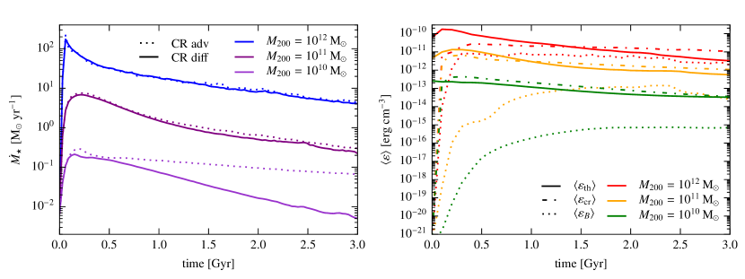
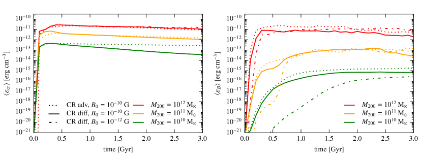
Figure 1: Time evolution of the SFR (top left-hand panel) and the volume-averaged energy densities in a disc of radius 10 kpc and total height 1 kpc (other panels). Different halo masses ($10^{10},~{}10^{11}$, and $10^{12}~{}\mathrm{M}_{\odot}$, all with concentration $c_{200}=12$) are colour coded. Simulations with advective and anisotropic diffusive CR transport (solid) suppress star formation more strongly in smaller galaxies in comparison to simulations that only account for CR advection (dotted). The top right-hand panel shows the time evolution of the thermal, CR and magnetic energy densities in our anisotropic CR diffusion model with an initial magnetic field $B_{\mathrm{init}}=10^{-10}\,\mathrm{G}$ and demonstrates that the magnetic saturation time scale increases for smaller galaxies and does not saturate at equipartition with the thermal energy density. In the bottom panels, we compare the CR (left) and magnetic energy density (right) for different simulations denoted in the bottom-left panel. While CR diffusion causes a net loss of CR energy from the disc, the initial magnetic field strength has no impact on the CR energy density. The magnetic energy density grows first exponentially (via a small-scale dynamo) and saturates in the following. Because of the finite turbulent driving time of the initial starburst and the larger magnetic growth time in smaller galaxies, the magnetic field in the simulations with $B_{\mathrm{init}}=10^{-12}\,\mathrm{G}$ increases at a much slower rate (dash-dotted).

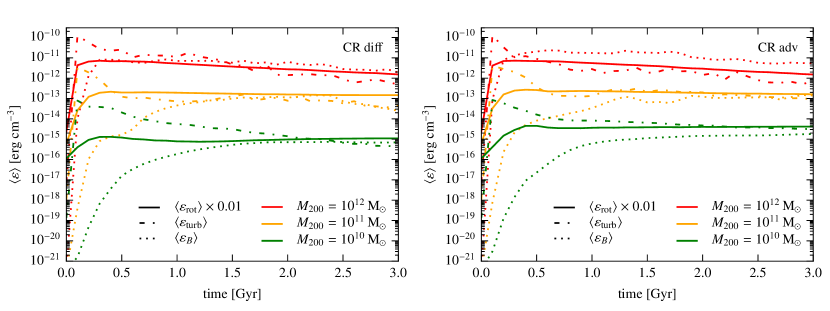
Figure 2: Halo mass dependence of the magnetic saturation level. We show the time evolution of the volume-averaged magnetic energy density (dotted), the kinetic rotational and ‘turbulent’ energy densities ($\varepsilon_{\mathrm{rot}}=\rho\varv_{\varphi}^{2}/2$, solid, and $\varepsilon_{\mathrm{turb}}=\rho\delta\varv^{2}/2\approx 3/4\times\rho(\varv_{z}^{2}+\varv_{R}^{2})$, dash-dotted) in a disc of radius 10 kpc and total height 1 kpc for our models ‘CR diff’ (left) and ‘CR adv’ (right). Simulations of different halo masses ($10^{10},~{}10^{11}$, and $10^{12}~{}\mathrm{M}_{\odot}$, all with concentration $c_{200}=12$, $B_{\mathrm{init}}=10^{-10}\,\mathrm{G}$ and $\zeta_{\mathrm{SN}}=0.05$) are colour coded. All discs are rotationally supported so that $\varepsilon_{\mathrm{rot}}\approx 100\varepsilon_{\mathrm{turb}}$ at late times. A small-scale dynamo amplifies the magnetic field so that it comes into equipartition with the ‘turbulent’ energy density after the initial growth phase. We see evidence for an additional magnetic amplification mechanisms in the $10^{12}~{}\mathrm{M}_{\odot}$ halo at late times.

3 Energy equipartition and the small-scale dynamo

First, we are studying the growth and saturation of CR and magnetic energy densities in comparison to the thermal and kinetic energy density across different halo masses. We will specifically work out the saturation level of the magnetic field strength with halo mass. We carefully explore the characteristics of the amplification mechanisms for galactic magnetic fields and identify adiabatic compression in the initial stage, followed by a superposition of small-scale dynamo processes to be responsible for magnetic field growth. This is supported by a discussion of the numerical Reynolds number in our moving mesh simulations. Power spectrum analyses and magnetic curvature statistics provide further insights into the kinematic and saturated regimes of the small-scale magnetic dynamo.

3.1 Growth and saturation of CR and magnetic energy densities

To mimic density inhomogeneities of cosmologically growing haloes in our idealised setup, we sample the softened NFW mass density profile randomly while ensuring equal mass per Voronoi cell. As a result, there is a distribution of mass densities at any given radius, which breaks the axisymmetry of our setup. At the beginning of our simulations, we switch on cooling of the slowly rotating gas in approximate hydrostatic equilibrium. As a result, the densest gas at the halo centre cools fastest, collapses and experiences adiabatic compression. A shock forms once later collapsing gas encounters the compressed dense gas at the centre. The (peanut-shaped) accretion shock propagates into the slightly inhomogeneous circumgalactic medium (see figure 5 of Springel & Hernquist, 2003) and thermalises the kinetic energy from gravitational infall, thereby reducing the gas velocities behind the shock. The accretion shock itself becomes corrugated as it interacts with the cooler and denser, filamentary infalling structures that have initially been sourced by small-scale overdensities. This leaves behind a hot and turbulent circumgalactic atmosphere because the curved shock converts a fraction of the angular momentum of the accreting gas into vorticity at the scale of the shock curvature according to Crocco’s theorem (1937). This vorticity cascades down in scale and feeds a turbulent kinetic power spectrum that will amplify any existing magnetic field as we will show in the following.

Conservation of specific angular momentum of the cooling gas causes a fraction of high angular momentum gas to be constantly accreted along the equatorial plane so that a centrifugally supported cool disc forms at around 150 Myr in the Milky Way-like halo and somewhat later in the dwarf galaxies. The cool galactic disc has a temperature of a few times $10^{5}$ K in our effective ISM model and typical sound speeds of several tens of $\mathrm{km~{}s}^{-1}$. This causes a supersonic velocity shear between the rotationally supported cool disc and the slower rotating and partially pressure supported hot circumgalactic medium at temperatures $\gtrsim 2\times 10^{6}$ K, which excites and grows Kelvin-Helmholtz surface and body modes (Mandelker et al., 2016; Berlok & Pfrommer, 2019a, b). As a result, turbulence is continuously injected at later times ($t\gtrsim 200$ Myr) through non-linearly interacting body modes on a range of scales at and below the scale of the vertical extend of the velocity shear. As we will show below, this causes a turbulent cascade, amplifies the magnetic fields further via a small-scale dynamo (which can be supplemented by a large-scale dynamo, Brandenburg & Subramanian, 2005) and is eventually dissipated at the grid scale.

The rotating cool disc provides favourable conditions for star formation so that all our simulations exhibit strong initial starbursts that are followed by exponentially declining SFRs in our large galaxies, independent of the CR transport scheme as well as in the $10^{10}\,\mathrm{M}_{\odot}$ halo in our model ‘CR diff’. By contrast, star formation starts to level off in the model ‘CR adv’ in this dwarf galaxy (top left-hand panel of Fig. 1). The behaviour is mirrored in the evolution of the CR energy density in the panel below. The reason of the suppressed SFR in small haloes are CR-driven winds that efficiently remove gas from the disc in the ‘CR diff’ model: after CRs have accumulated in the disc, their buoyancy bends and opens up the toroidal disc magnetic field. CRs diffuse into the halo and accelerate the gas, thereby driving an outflow solely through the CR pressure gradient force with increasing strength towards smaller galaxies (see also Jacob et al., 2018, for a study of the halo-mass dependence of CR feedback). We find only weak fountain flows in model ‘CR adv’ (see also Pakmor et al., 2016c).

The top right-hand panel of Fig. 1 shows the time evolution of the average thermal, CR and magnetic energy densities in model ‘CR diff’. After the starburst, the injection of CR energy at SNRs quickly causes the CRs to reach approximate equipartition with the thermal energy (top right-hand panel of Fig. 1). While CR and thermal energies balance each other in the $10^{10}\,\mathrm{M}_{\odot}$ halo, the CR component quickly dominates the overall energy budget in larger galaxies to the point where it triples the thermal energy in the Milky Way-mass galaxy. Note that these energy densities represent averages in a disc of radius 10 kpc and total height 1 kpc and that the individual pressures vary with galactocentric radius and height from the disc. While our simulations predict that CR and thermal pressures reach equipartition at the solar radius in our Milky Way-mass galaxy, they dominate over the thermal pressure at larger radius and disc heights while they fall short of the thermal pressure at smaller radii (see figure 1 of Pfrommer et al. 2017b).

The approximate equipartition of CR and thermal energy density (within a factor of three) is a direct consequence of CR physics and our pressurised ISM (Springel & Hernquist, 2003), which models the multi-phase ISM with an effective equation of state so that it balances the vertical disc gravity. In fact, the approximate equipartition suggests an attractor solution of a self-regulated feedback loop: if the CR pressure accumulates until CRs dominate the energy budget, they will buoyantly and diffusively escape into the halo and push on the gas by means of their gradient pressure force. Conversely, if thermal pressure dominates, it will loose its energy radiatively at a much faster rate in comparison to magnetic fields and CRs, which have negligible radiative losses and experience losses due to inelastic collisions with the ambient gas (Jubelgas et al., 2008). This self-regulation picture implies a robust physical attractor solution that our simulations seem to settle into, but to which extend this attractor is realised and understanding the conditions for its violations needs to be studied with CR hydrodynamics in the self-confinement picture (Thomas & Pfrommer, 2019; Thomas et al., 2022).

In the first stage of our simulations, the magnetic energy density $\varepsilon_{B}$ grows exponentially across more than ten orders of magnitude, which is followed by slower growth until $\varepsilon_{B}$ eventually saturates. The top right-hand panel of Fig. 1 shows a smaller growth rate in smaller galaxies which leads to a saturation level below equipartition in these dwarf galaxies. We find saturation times of 0.3 Gyr and 1.5 Gyr for our haloes with masses $10^{12}$ and $10^{11}~{}\mathrm{M}_{\odot}$ in model ‘CR diff’. In addition, the strong outflow in the $10^{10}~{}\mathrm{M}_{\odot}$ halo in model ‘CR diff’ quenches the dynamo, which reaches a saturated mean field ${\langle}B\rangle=\sqrt{8\uppi{\langle}\varepsilon_{B}\rangle}\approx 0.1~{}\upmu$G (averaged over the disc and after 3 Gyr), which is three times lower than in model ‘CR adv’ (Pfrommer et al., 2017a). It is interesting to note that already in the $10^{11}~{}\mathrm{M}_{\odot}$ halo, the mean magnetic energy density saturates below that of the CMB,

$$\varepsilon_{\mathrm{CMB}}=\frac{\uppi^{2}}{15}\,\frac{(k_{\mathrm{B}}T_{\mathrm{CMB}})^{4}}{(\hbar c)^{3}}(1+z)^{4}\approx 4.17\times 10^{-13}(1+z)^{4}~{}\mathrm{erg~{}cm}^{-3}$$ (10)

where $k_{\mathrm{B}}$ is Boltzmann’s constant, $T_{\mathrm{CMB}}=2.725$ K, $\hbar$ is the reduced Planck’s constant, and $z$ denotes the cosmic redshift. This implies that CR electrons in low-mass galaxies cool primarily via IC interactions on CMB photons rather than on FIR photons or via synchrotron emission.

Most importantly, we observe that the magnetic field strength in galaxies smaller than the Milky Way saturates at values significantly below equipartition with the thermal pressure. Figure 2 shows that the evolution of the magnetic energy density saturates approximately in equipartition with the poloidal kinetic energy density that is a proxy for the ‘turbulent’ energy density driven by gravitational collapse and non-linearly interacting Kelvin-Helmholtz body modes in the disc, $\varepsilon_{\mathrm{turb}}=\rho\delta\varv^{2}/2\approx 3/4\times\rho(\varv_{z}^{2}+\varv_{R}^{2})$, where $\rho$ is the gas mass density. Initially, the accretion shock converts the radial infall velocities into thermal energy and turbulence, which is visible as a peak in $\varepsilon_{\mathrm{turb}}$ at 0.1 Gyr, after which time the accretion shock leaves the vertical extent of the cylindrical averaging region. In consequence, the poloidal kinetic energy density decreases because gas accretion and the associated turbulent driving become weaker. However, the velocity shear associated with the fast rotating galactic disc in the hot circumgalactic medium maintains continuous turbulent driving and explains the approximately constant $\varepsilon_{\mathrm{turb}}$, as will be explicitly shown in Section 3.2 (see also figure 6 of Berlok & Pfrommer, 2019b).

As we will show in Section 3.3, a small-scale dynamo exponentially amplifies the magnetic field so that it comes into approximate equipartition with the gravo-turbulent energy density. A fraction of the initial potential energy of the halo gas feeds the gravo-turbulence and hence drives the small-scale dynamo either through the corrugated accretion shock or via the velocity shear between hot circumgalactic medium and cool disc. In this picture, we would expect that the saturated level of magnetic energy scales as

$$E_{B}\sim E_{\mathrm{turb}}\sim\frac{\eta\,M_{200}\,\varv_{200}^{2}}{2}\propto M_{200}^{5/3},$$ (11)

where $\varv_{200}=\sqrt{GM_{200}/r_{200}}$ is the virial velocity and $\eta$ is an energy conversion efficiency. In fact, this halo mass scaling is consistent with our findings in Fig. 2, in which we find magnetic energy densities in our ‘CR diff’ model (at 3 Gyr) of $\varepsilon_{B}\sim\{9\times 10^{-16},4\times 10^{-14},2\times 10^{-12}\}~{}\mathrm{erg~{}cm}^{-3}$ for the $10^{10},~{}10^{11}$, and $10^{12}~{}\mathrm{M}_{\odot}$ haloes, implying that $\eta$ is independent of halo mass in our simulations. Moreover, we see evidence for an additional magnetic amplification mechanism over the small-scale dynamo in the $10^{12}~{}\mathrm{M}_{\odot}$ halo after 1.5 Gyr (0.3 Gyr) in the ‘CR diff’ (‘CR adv’) model, that is stronger in the ‘CR adv’ model and consistent with a large-scale dynamo (Pakmor et al., 2016c). This is expected because CR (an-)isotropic diffusion is known to suppress any magnetic dynamo action because active CR transport (via diffusion or streaming) causes magnetised plasma to move off of the disc via CR pressure-gradient driven outflows, and carries magnetic flux alongside into the circumgalactic medium so that this would have to be replenished by the dynamo and decreases its overall efficiency in the disc (Pakmor et al., 2016c).

Note that our model underestimates supernova-driven turbulence because we only directly inject CR energy in a way that can drive locally expanding bubbles while we account for the remaining supernova energy in our effective equation of state of the ISM. Accounting for this additional local energy injection may be able to further amplify magnetic fields (Rieder & Teyssier, 2016, 2017a; Butsky et al., 2017). We also find that our discs are rotationally supported so that the kinetic rotational energy density $\varepsilon_{\mathrm{rot}}=\rho\varv_{\varphi}^{2}/2\approx 100\varepsilon_{\mathrm{turb}}$ at late times so that $\varepsilon_{\mathrm{rot}}\approx 3\varepsilon_{\mathrm{th}}$ in the $10^{10}~{}\mathrm{M}_{\odot}$ halo and $\varepsilon_{\mathrm{rot}}\approx 50\varepsilon_{\mathrm{th}}$ in the $10^{12}~{}\mathrm{M}_{\odot}$ halo in our ‘CR diff’ model. This explains the puffed-up appearance of dwarfs and the flattened disc-like morphology of our Milky Way-mass galaxies. In order to separate the various processes of magnetic field growth, we now analyse the correlation between gas density and magnetic field and quantify the scaling of the magnetic growth rate with Reynolds number.

3.2 Magnetic growth via adiabatic compression and the small-scale dynamo

Figure 3: Mass-weighted probability density of magnetic field strength, $B$, and mass density, $\rho$, for our high-resolution Milky Way-like halo of mass $10^{12}~{}\mathrm{M}_{\odot}$ and concentration $c_{200}=12$. From left to right, the panels show three characteristic phases of magnetic field growth: (i) adiabatic growth phase, (ii) exponential growth phase in the kinematic regime (as will be shown in Fig. 4), and (iii) growth of magnetic coherence scale (as will be demonstrated in Section 3.3). All gas densities are scaled to the star formation threshold $\rho_{0}=4.05\times 10^{-25}\,\mathrm{g~{}cm}^{-3}$. The initial distributions are shown with a dash-dotted line while the adiabatically compressed magnetic field follows $B\propto\rho^{2/3}$ for isotropic collapse (dotted line). Note that the small-scale dynamo starts to grow the field above the adiabatically compressed value at around $t\approx 0.07$ Gyr.

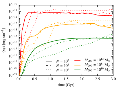
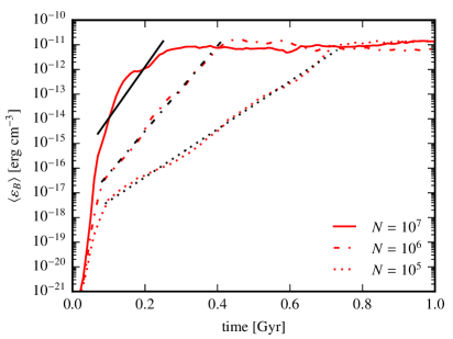
Figure 4: Time evolution of the volume-averaged magnetic energy densities in a disc of radius 10 kpc and total height 1 kpc. Different halo masses ($10^{10},~{}10^{11}$, and $10^{12}~{}\mathrm{M}_{\odot}$, all with concentration $c_{200}=12$) are colour coded and different numerical resolution levels are shown with different line styles. The panel on the left-hand side shows the overall evolution while the panel on the right-hand side shows a zoom on the $10^{12}~{}\mathrm{M}_{\odot}$ halo at early times and additionally exponential fits to the exponential growth phase following the initial adiabatic compression phase. This demonstrates that the dynamo starts earlier and the exponential growth rate is larger for increasing resolution and halo masses.

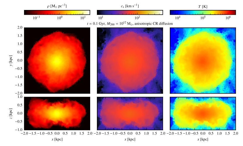
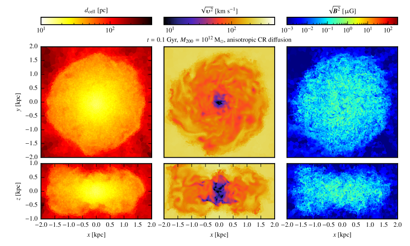
Figure 5: Properties of the central region in our Milky Way-mass galaxy ($M_{200}=10^{12}~{}\mathrm{M}_{\odot}$, $c_{200}=7$) during the exponential growth phase in the kinematic regime at $t=0.1$ Gyr. We show cross-sections in the mid-plane of the disc (face-on views) and vertical cut-planes through the centre (edges-on views) of the gas mass density, sound speed and temperature (top panels, from left to right) and the Voronoi cell diameters $d_{\mathrm{cell}}$, gas velocity and magnetic field strength (bottom panels). The corrugated accretion shock dissipates kinetic energy from gravitational infall into heat, induces turbulence with an outer scale of $\mathscr{L}\approx 1$ kpc, and drives a small-scale dynamo.

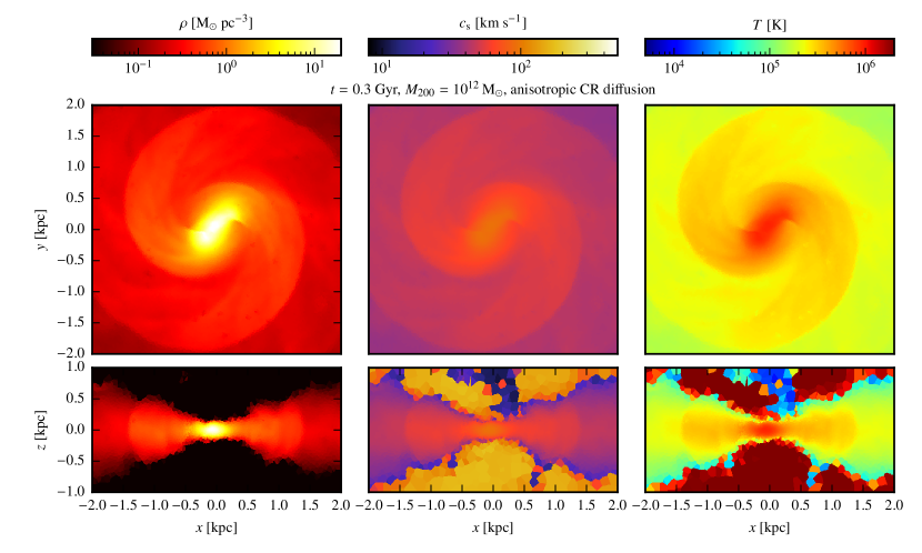
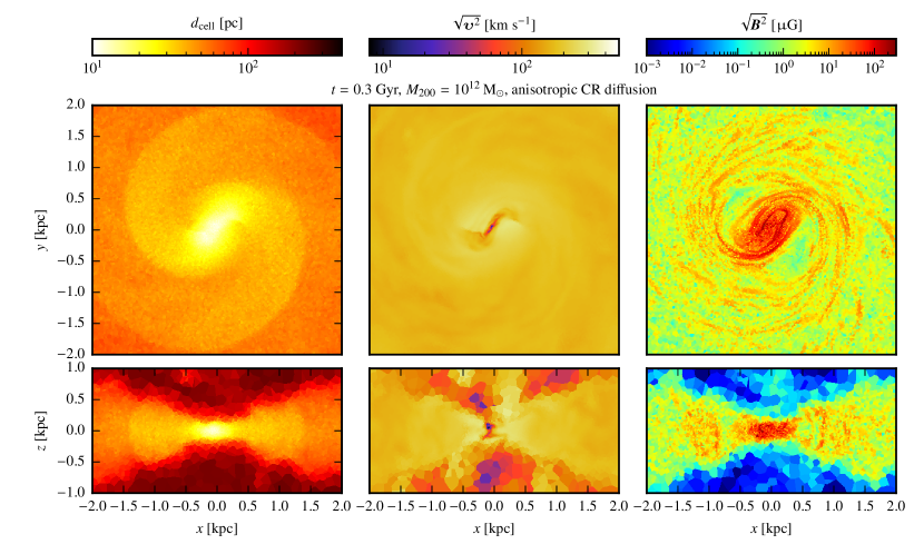
Figure 6: Properties of the central region in our Milky Way-mass galaxy ($M_{200}=10^{12}~{}\mathrm{M}_{\odot}$, $c_{200}=7$) after saturation of the dynamo on small scales while the magnetic coherence scale increases (at $t=0.3$ Gyr). As in Fig. 5, we show gas mass density, sound speed and temperature (top panels, from left to right) and the Voronoi cell diameters $d_{\mathrm{cell}}$, gas velocity and magnetic field strength (bottom panels), all with identical colour scales as in Fig. 5. There is a supersonic velocity shear between the rotationally supported cooler disc and the slower rotating and hotter circumgalactic medium that excites Kelvin-Helmholtz body modes (with a characteristic outer scale of turbulence of $\mathscr{L}\approx 1$ kpc). Non-linear interactions of these modes also drive a small-scale dynamo in the disc.

First, we explore the correlation of magnetic field strength, $B$, and gas density, $\rho$, during the initial stages of the simulation of our Milky Way-like halo of mass $10^{12}~{}\mathrm{M}_{\odot}$ and concentration $c_{200}=12$. After the onset of cooling and the associated gravitational collapse, the initial magnetic field is adiabatically compressed. The isotropic collapse toward the halo centre causes the initial magnetic field to increase and to scale with the gas density as $B\propto\rho^{2/3}$ (see left-hand panel of Fig. 3). At around $t=0.07$ Gyr, the central region has settled to the ISM density so that the gas is not any more adiabatically compressed. Instead, the small-scale dynamo continues to grow the magnetic field. Because it acts fastest at the smallest turbulent eddies, which are best resolved at the highest densities in our quasi-Lagrangian simulation, at $t=0.1$ Gyr the magnetic field is clearly elevated over the adiabatic scaling at densities $\rho\gtrsim 100\rho_{0}$ (see middle panel of Fig. 3).

Once the small-scale magnetic power saturates (at a large fraction of the kinetic power), the coherence scale of the magnetic field grows to progressively larger scales (as will be shown in Section 3.3) and correspondingly lower gas densities. This can be seen in the right-hand panel of Fig. 3 (at $t=0.2$ Gyr), which shows a departure of the dynamo-grown field over the adiabatically compressed one already at densities $\rho\gtrsim\rho_{0}$. Soon thereafter, the field saturates in equipartition with the turbulent energy (cf. Fig. 2). The shape of the $B$–$\rho$ correlation at saturation does not depend on our specific choice of magnetic initial conditions as we explicitly show in Fig. 24, where we compare our constant initial field to a dipole configuration of an adiabatically pre-compressed field. Figure 24 shows that deep in the saturated regime of magnetic field growth (i.e., well after the starburst), most gas at $\rho\gtrsim 10\rho_{0}$ has been converted to stars, implying a much reduced probability density in comparison to the starburst phase studied in Fig. 3. Alongside this conversion, our subgrid model assumes that the flux-frozen magnetic field is also locked up in those stars, thereby reducing the disc magnetic field.

To study the initial magnetic growth phase, we compare the time evolution of the magnetic energy density, $\varepsilon_{B}$, averaged across the disc (of radius 10 kpc and total height 1 kpc) in haloes of different masses and numerical resolution (left-hand panel of Fig. 4), but with identical concentrations so that the halo profiles are exact gravitational replicas of each other at different masses. Clearly, increased numerical resolution at each halo mass enables us to resolve smaller eddies and hence faster magnetic growth rates. While the saturation level of $\varepsilon_{B}$ is converged for $N\geq 10^{6}$ initial resolution elements, the simulations with initially $N=10^{5}$ cells overproduces $\varepsilon_{B}$ by a significant amount.

The right-hand panel of Fig. 4 shows a zoom on the $10^{12}~{}\mathrm{M}_{\odot}$ halo at early times. We see an initial exponential growth of the magnetic field due to adiabatic compression of the seed magnetic field. Provided the cooling time is shorter than the gravitational free-fall time-scale, collapse and the associated adiabatic compression happens at the free-fall time, which is identical for the simulations at different numerical resolutions of a given halo and thus nearly independent of resolution. Subsequently, we see the already discussed magnetic growth at high densities: the onset of this second, exponential growth phase depends on resolution and starts at 50–80 Myr (corresponding to $N=10^{7}$ and $N=10^{5}$, respectively). Most importantly, the growth rate of this small-scale dynamo strongly depends on resolution and also follows an exponential growth:

$$\varepsilon_{B}(t)=\varepsilon_{B,0}\,\mathrm{e}^{\Gamma_{B}t}.$$ (12)

For our simulations with an initial number of Voronoi cells of $N=\{10^{5},\,10^{6},\,10^{7}\}$, we measure the exponential growth rate $\Gamma_{B}=\{22.4,\,39.8,\,48.0\}~{}\mathrm{Gyr}^{-1}$, which corresponds to a growth time of $\tau_{B}=\Gamma_{B}^{-1}=\{44.6,\,25.1,\,20.8\}~{}\mathrm{Myr}$. This basic picture of resolution dependent growth remains robust to changes of the averaging region, from a cylindrical disc to a sphere of different radii ($r_{\mathrm{s}}=\{1,0.5,0.25\}$ kpc) while the resulting growth rates are subject to larger Poisson fluctuations as a result of the lower number of cells for the smaller integration volumes.

The magnetic growth curve for the $10^{12}~{}\mathrm{M}_{\odot}$ halo of the high-resolution simulation ($N=10^{7}$) shows a distinct feature at 0.2 Gyr, which corresponds to the time-scale of the formation of the rotationally supported cool disc. This comes about because at this time, the outward propagating accretion shock is unable to maintain a powerful turbulent driving in the centre, which slows down the growth rate of the small-scale dynamo. However, the formation of the cooling disc generates a large velocity shear between the fast rotating disc and the slower rotating halo gas, which continuously injects fresh and powerful turbulence that is able to re-ignite the small-scale dynamo (as we will show below). The later onset of the small-scale dynamo in the lower resolution simulations (with $N\leq 10^{6}$) causes a blending of the two effects, which therefore cannot any more be separated in the time evolution of the average magnetic energy.

This interpretation is supported by Fig. 5, which shows the properties of the proto-galaxy during the exponential growth phase. The corrugated accretion shock dissipates kinetic energy from gravitational infall and heats the assembling galaxy to temperatures in excess of $2\times 10^{5}$ K corresponding to sound speeds of $50~{}\mathrm{km~{}s}^{-1}$. Most importantly, the velocity panels of Fig. 5 show that the curved shock decelerates the supersonic infall and injects vorticity. Interacting eddies generate subsonic turbulence, which cascades kinetic energy down in scale to the mesh size $d_{\mathrm{cell}}$, which is rather homogeneous behind the accretion shock and assumes the smallest values at the densest centre. As we will further argue below, this kinetic turbulence drives the small-scale dynamo and grows the magnetic field as can be seen in the bottom right-hand panels of Fig. 5. With increasing distance from the shock, turbulence decays as can be inferred from the velocity maps in the galactic centre.

Once the accretion shock propagates outwards and more gas accretes in the equatorial plane, it cools and forms a cooling and rotationally supported disk several tens of Myrs later (Fig. 6). This implies a large velocity shear between the fast rotating, radiatively cooling disc and the slower rotating and hotter circumgalactic medium that has been thermalised by the outwards propagating accretion shock. Locally, this situation can be identified with a cold stream moving supersonically through a hot, dilute circumgalactic medium, which is known to excite the Kelvin-Helmholtz instability in the hydrodynamic case (Mandelker et al., 2016, 2020; Padnos et al., 2018) as well as in the MHD case (Berlok & Pfrommer, 2019a, b). In the supersonic regime, the Kelvin-Helmholtz instability not only manifests itself by exciting the well-known surface modes but also by exciting reflective or body modes as (magneto-)acoustic waves reflect at the interface of the dense stream to the dilute background, thus trapping the acoustic wave energy within the stream. As a result, the waves grow in amplitude inside the stream (or in our case the rotationally supported cool disc). This excites a broad spectrum of unstable wave modes that grow into the non-linear regime and interact with each other to inject subsonic turbulence, which further amplifies the magnetic field through a second small-scale dynamo mode (bottom panels of Fig. 6). Note that gravitational collapse of dense gas clouds, star formation, energetic feedback and the centrifugal force in the rotating frame modify the late-time behaviour of the non-linearly saturating dynamo in comparison to the idealised simulations of supersonically moving cold streams.

Using typical shear velocities of $\mathscr{V}\sim\mbox{(50$-$100)}~{}\mathrm{km~{}s}^{-1}$ across a scale of $\mathscr{L}\sim 1~{}\mathrm{kpc}$ (bottom panels of Fig. 6), where the lower (upper) value characterises an average (maximum) shear, we can estimate the turbulent energy dissipation rate at the Kolmogorov scale, $\varv_{\ell}^{3}/\ell\sim\mathscr{V}^{3}/\mathscr{L}\sim\mbox{(0.7$-$5)}\times 10^{-25}~{}\mathrm{erg~{}s}^{-1}\,m_{\mathrm{p}}^{-1}$. To order of magnitude, this energy rate is generated on the vertical sound crossing time, characterised by the thermal velocity $\varv_{\mathrm{th}}\sim 50~{}\mathrm{km~{}s}^{-1}$ (in our ISM subgrid model, see Fig. 6) and implying a dissipated energy density $\varepsilon_{\mathrm{diss}}\sim\rho\mathscr{V}^{3}/\varv_{\mathrm{th}}\sim(2\times 10^{-9}-2\times 10^{-7})~{}\mathrm{erg~{}cm}^{-3}$. This corresponds to equivalent magnetic field strengths of $B_{\mathrm{diss}}\sim\mbox{(200$-$2000)}~{}\upmu$G available for tapping in by the small-scale dynamo. Here, we use characteristic density values of $80~{}\mathrm{cm}^{-3}$ ($800~{}\mathrm{cm}^{-3}$) for the outer (inner) disc in our simulations, respectively, which amounts to mass densities of $1~{}\mathrm{M}_{\odot}~{}\mathrm{pc}^{-3}$ ($10~{}\mathrm{M}_{\odot}~{}\mathrm{pc}^{-3}$), see Fig. 6. These equivalent magnetic field strengths are about a factor of 20 larger than the realised magnetic field strengths $B\sim\mbox{(10$-$100)}~{}\upmu$G in our simulations (Fig. 6) and substantially larger than the volume-averaged magnetic energy density $\varepsilon_{B}\sim 10^{-11}~{}\mathrm{erg~{}cm}^{-3}$ in the disc (Fig. 2).

Our simulations solve the equations of ideal MHD, i.e., we do not explicitly model physical viscosity and resistivity. Moreover, our simulations can only resolve dynamo growth on scales larger than our numerical Voronoi grid, which is substantially coarser in comparison to the astrophysical magnetic resistive scale and therefore, our simulated magnetic fields grow much slower in comparison to the astrophysical case. Thus, numerical viscosity and resistivity determine the growth rate of the small-scale dynamo. Employing the scaling properties of Kolmogorov turbulence (see Appendix A.1), we expect a growth rate in the kinematic regime of the small-scale dynamo (which is equal to the eddy turnover rate at the dissipation scale for a magnetic Prandtl number of unity) of

$$\Gamma=\frac{\mathscr{V}}{\mathscr{L}}\,\mathrm{Re}^{1/2},$$ (13)

where $\mathscr{L}$ and $\mathscr{V}$ are the length and velocity scale at the turbulent injection scales and Re is the physical Reynolds number, which is given by

$$\mathrm{Re}=\frac{\mathscr{L}\mathscr{V}}{\nu_{\mathrm{vis}}}\sim\frac{3\mathscr{L}\mathscr{V}}{\lambda_{\mathrm{mfp}}\varv_{\mathrm{th}}},$$ (14)

where $\nu_{\mathrm{vis}}\sim\lambda_{\mathrm{mfp}}\varv_{\mathrm{th}}/3$ is the kinetic viscosity, $\lambda_{\mathrm{mfp}}$ is the particle mean free path, and $\varv_{\mathrm{th}}$ is the thermal velocity. Thermal particles moving a mean free path collide and randomise their velocities, which implies that $\lambda_{\mathrm{mfp}}$ is the typical length over which the fluid can communicate changes in its shear stress. A fluid with a longer mean free path therefore more easily opposes changes to its local shear velocity, i.e., is more viscous. By analogy with this property, we define the numerical Reynolds number via

$$\mathrm{Re}_{\mathrm{num}}\equiv\frac{\mathscr{L}\mathscr{V}}{\nu_{\mathrm{num}}}\sim\frac{3\mathscr{L}\mathscr{V}}{d_{\mathrm{cell}}\varv_{\mathrm{sig}}},$$ (15)

where $\nu_{\mathrm{num}}$ is the numerical viscosity and $d_{\mathrm{cell}}=(6V/\uppi)^{1/3}$ is the diameter of the smallest characteristic Voronoi cell (assuming a spherical cell volume $V$), i.e., it is abundantly present in a singly connected region so that it governs therein the numerical dissipation properties. The signal speed of the gas relative to the numerical mesh, $\varv_{\mathrm{sig}}$, differs among the various computational techniques. For a spatially fixed mesh (homogeneous or adaptive Eulerian), the signal velocity is the sum of bulk velocity relative to the mesh and thermal velocity, $\varv_{\mathrm{sig}}=\mathscr{V}+\varv_{\mathrm{th}}$, so that the numerical Reynolds number for Eulerian techniques is given by

$$\mathrm{Re}_{\mathrm{num,\,Euler}}\sim\frac{3\mathscr{L}}{d_{\mathrm{cell}}}\,\frac{\mathscr{V}}{\mathscr{V}+\varv_{\mathrm{th}}}\sim\frac{3\mathscr{L}}{2d_{\mathrm{cell}}},$$ (16)

where we adopted the transsonic case $\mathscr{V}\approx\varv_{\mathrm{th}}$ in the last step, which is relevant for a small-scale dynamo in galactic discs that are excited through Kelvin-Helmholtz surface and body modes evolving into the non-linear regime (Berlok & Pfrommer, 2019a, b). However, for a quasi-Lagrangian code where the mesh moves close to the speed of the gas, we have $\varv_{\mathrm{sig}}\approx\varv_{\mathrm{th}}$ so that we obtain

$$\mathrm{Re}_{\mathrm{num,\,Lagrange}}\sim\frac{3\mathscr{L}}{d_{\mathrm{cell}}}\,\frac{\mathscr{V}}{\varv_{\mathrm{th}}}\sim\frac{3\mathscr{L}}{d_{\mathrm{cell}}},$$ (17)

where we also adopted the transsonic case $\mathscr{V}\approx\varv_{\mathrm{th}}$ in the last step and which is larger by a factor of two in comparison to the Eulerian case. To avoid mesh twisting and large gradients in mesh resolution, Arepo moves the generating points relative to the gas with a velocity that is typically small in comparison to $\varv_{\mathrm{th}}$ for a galaxy simulation that does not resolve the cold molecular phase.

To estimate $\mathrm{Re}_{\mathrm{num}}$, we adopt a cell diameter $d_{\mathrm{cell}}\approx 10$ pc appropriate for the fastest growing magnetic field in the centre (Fig. 20) and a thermal velocity of our star-forming subgrid ISM at $2\times 10^{5}$ K of $\varv_{\mathrm{th}}\approx 50~{}\mathrm{km~{}s}^{-1}$. We approximate the outer scale of turbulence by $\mathscr{L}\approx 1$ kpc, which is the characteristic length scale of the initial accretion shock (Fig. 5) and also corresponds to the scale of the thick disc (Fig. 6). To estimate the injection velocity at the outer scale, we note that in both scenarios discussed (an exponentially growing small-scale dynamo in the post-shock regime of the initial accretion shock as well as the non-linearly growing Kelvin-Helmholtz instability), we expect $\mathscr{V}\approx\varv_{\mathrm{th}}$. As a result, we find a typical value of $\mathrm{Re}_{\mathrm{num}}\sim 3\times 10^{2}$. Thus, we obtain turbulent velocities of $\varv_{\ell}=\mathscr{V}\,\mathrm{Re}_{\mathrm{num}}^{-1/4}\approx 12~{}\mathrm{km~{}s}^{-1}$ (Eq. 46) at the resolution scale $\ell$ in the galaxy centre. The eddy turnover rate at this (numerical) Kolmogorov scale is:

$$\Gamma\sim\frac{\varv_{\ell}}{2\uppi\,r_{\mathrm{eddy}}}\sim 65~{}\mathrm{Gyr}^{-1}\approx 1.35\,\Gamma_{B},$$ (18)

where we assume that the smallest turbulent eddies are starting to be resolved for a radius that extends across three cells, $r_{\mathrm{eddy}}=3d_{\mathrm{cell}}$ and $\Gamma_{B}=48~{}\mathrm{Gyr}^{-1}$ is the measured exponential growth rate of the magnetic field of our high-resolution simulation (Eq. 12). This theoretically expected growth rate is 35 per cent larger than the measured value because of numerical dissipation and because stars represent sinks of magnetic energy in our model, thereby reducing the dynamo efficiency in comparison to the theoretical maximum. Clearly, astrophysical Reynolds numbers for an accretion-driven dynamo in proto-galaxies are of order $\mathrm{Re}\sim 10^{11}$, implying growth times that are a factor $2\times 10^{4}$ shorter (Schober et al., 2013).

If we re-normalise the numerical growth rates to the simulation with the lowest resolution, $\Gamma_{B,5}=22.4~{}\mathrm{Gyr}^{-1}$ (where $\Gamma_{B,5}$ denotes $\Gamma_{B}$ of our $N=10^{5}$ simulation), we would expect to obtain growth rates of $\Gamma_{B,6}=\Gamma_{B,5}10^{1/6}=32.9~{}\mathrm{Gyr}^{-1}$ (a factor 0.83 smaller than the measured growth rate) and $\Gamma_{B,7}=\Gamma_{B,5}10^{1/3}=48.2~{}\mathrm{Gyr}^{-1}$ (consistent with the measured growth rate). This excellent agreement of simulations and small-scale dynamo theory is reassuring that our MHD solver produces reliable results and provides support of the picture that the small-scale dynamo grows the magnetic field after an initial phase of adiabatic compression. To understand the scale dependence of the magnetic dynamo, we now turn to a power spectrum analysis.

3.3 Power spectrum analysis of the small-scale dynamo

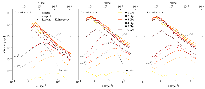
Figure 7: Comparison of kinetic (solid) and magnetic (dashed) power spectra for different analysis regions (indicated in the top left) for the ‘CR diff’ simulation of the $10^{12}~{}\mathrm{M}_{\odot}$ halo with $c_{200}=7$ and $B_{\mathrm{init}}=10^{-10}$G. The kinetic energy power spectrum decays with time because the thermal and CR pressure that surround the forming disc slows gravitational infall onto the disc and the Kelvin-Helmholtz driven turbulence weakens with time. On the contrary, the magnetic power spectrum grows exponentially until it saturates on small scales while it grows further on larger scales, implying a shift of the coherence scale to larger scales. The black dotted lines show the slopes of a Kazantsev (1968) spectrum ($\propto k^{3/2}$) in the kinematic regime at large scales and a Kolmogorov (1941) spectrum ($\propto k^{-5/3}$), which is theoretically expected at non-linear scales in a small-scale dynamo and realised in our simulation if we omit all gas cells in the central 1 kpc sphere (right-hand panel). When we include the central region (left-hand and middle panels), the magnetic power spectrum follows a Lorentzian function on large scales, which is the Fourier transform of the exponential magnetic profile with scale length $r_{0}=2\uppi/k_{0}=0.4$ kpc. The power of this profile is then cascaded to smaller scales with a rate given by MHD turbulence theory (dash-dotted, see Eq. 20).

Initially weak seed magnetic fields can be amplified due to stretching, twisting and folding of field lines driven by turbulent eddies (Zeldovich et al., 1983; Childress & Gilbert, 1995), where the exponential amplification time is given by the turbulent eddy turnover time. For weak seed magnetic fields, the kinematic limit applies and we expect a scaling of the magnetic energy spectrum $P(k)\mathrm{d}k\propto k^{3/2}\mathrm{d}k$ according to the dynamo theory by Kazantsev (1968). Provided the initial magnetic energy is smaller than the kinetic energy of the smallest turbulent eddies and neglecting compressible effects, we can apply the Kazantsev theory to the entire inertial range of turbulence between the injection scale and viscous cut-off scale.

In order to study whether our galaxy simulations grow the magnetic field through this mechanism, we plot the evolution of the magnetic and kinetic power spectra in Fig. 7. Following Pakmor et al. (2017, 2020), we compute these power spectra by taking the absolute square of the Fourier components of $\sqrt{\rho}\,\bm{\varv}$ and $\bm{B}/\sqrt{8\uppi}$, respectively, for gas within a sphere of radius $r_{\mathrm{s}}=1$ and 5 kpc (indicated in the legends of Fig. 7). This is done within a zero-padded box of size $\pm 2r_{\mathrm{s}}$ across so that the fundamental mode has a wavelength of 4 and 20 kpc, respectively. Accordingly, drops in the power spectra on scales greater than 2 and 10 kpc are an artefact of this zero-padding. By considering only gas within 1 and 5 kpc of the galactic centre, we isolate the regions in which the greatest amplification takes place.

After the kinematic magnetic power spectrum has been exponentially amplified to the point where the magnetic and turbulent energy of the smallest eddies have achieved equipartition, the back-reaction through the magnetic tension force is strong enough to suppress the stretching process of these eddies at the equipartition scale. On larger scales, the magnetic power spectrum continues to be amplified to the equipartition scale of the corresponding modes with a slower growth rate. Because in Kolmogorov turbulence, there is more turbulent kinetic energy available on larger scales, the magnetic energy grows to a larger amplitude. Hence, the magnetic coherence scale grows as a function of time, which appears like inverse cascade but in fact, it does not represent an inverse cascade in its strict definition because there are no integrals of motion in a fluctuating dynamo, which would necessarily create an inverse cascade.

On scales smaller than the current equipartition scale, we are entering the non-linear stage of the small-scale dynamo, that is characterised by an equipartition of magnetic and turbulent kinetic energy so that the initially hydrodynamic turbulence is modified to become MHD turbulence (Goldreich & Sridhar, 1995). Until the kinetic injection scale has reached the equipartition condition, we observe in Fig. 7 a co-existence of the kinematic dynamo spectrum on large scales and a spectrum $P(k)\mathrm{d}k\propto k^{-5/3}\mathrm{d}k$ on scales smaller than the equipartition scale (Brandenburg & Subramanian, 2005).

In our case, the dark matter gravitational potential causes a density stratification on which the kinetic and magnetic turbulence is imprinted. The turbulence is driven by rotational gravitational infall, cooling and star formation. The power spectrum probes thus the combination of the large-scale density and magnetic profiles and turbulent fluctuations on smaller scales. The three-dimensional distribution of the root-mean square magnetic field strength obeys a steep exponential profile in the centre at early times, $B(r)=B_{0}\mathrm{e}^{-k_{0}r}$, where $r=\sqrt{\textbf{{x}}^{2}}$ is the spherical radius and $k_{0}=2\uppi/r_{0}$ is the wavenumber corresponding to the scale length $r_{0}$ of the exponential magnetic profile (see Fig. 21). The Fourier transformation of the exponential ‘form factor’ is given by the Lorentzian profile in wave number, $k=|\textbf{{k}}|$,

$$\mathcal{F}\left(\mathrm{e}^{-k_{0}r}\right)(k) =\int_{-\infty}^{\infty}\mathrm{d}^{3}x\,\mathrm{e}^{-k_{0}\sqrt{x^{2}+y^{2}+z^{2}}}\mathrm{e}^{-\mathrm{i}\textbf{{k}}\bm{\cdot}\textbf{{x}}}$$

$$=4\uppi\int_{0}^{\infty}\mathrm{d}rr^{2}\mathrm{e}^{-k_{0}r}\frac{\sin(kr)}{kr}=\frac{8\uppi k_{0}}{(k^{2}+k_{0}^{2})_{\phantom{0}}^{2}}.$$ (19)

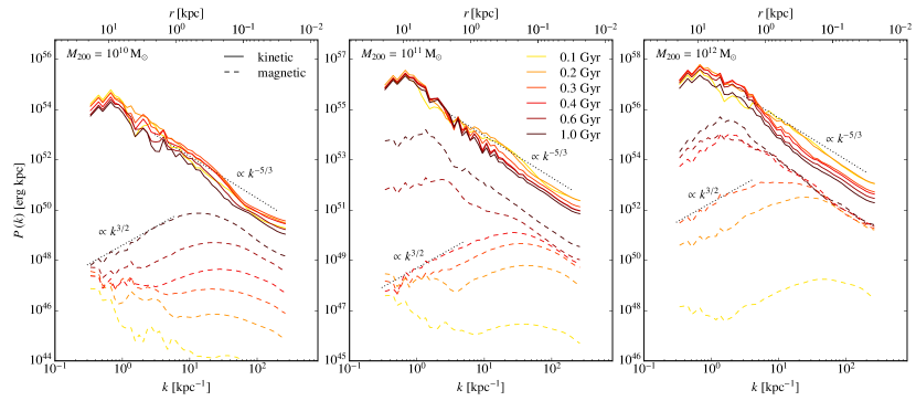
Figure 8: Comparison of kinetic and magnetic power spectra for different halo masses ($10^{10},~{}10^{11}$, and $10^{12}~{}\mathrm{M}_{\odot}$, all with a concentration parameter $c_{200}=12$, $B_{\mathrm{init}}=10^{-10}$G, and the model with advective and anisotropic diffusive CR transport). We compute the power spectra in a spherical shell bounded by $1<r/\mathrm{kpc}<5$. The larger concentration parameter in comparison to $c_{200}=7$ used in the analysis of Fig. 7 causes a larger adiabatic compression of $B_{\mathrm{init}}$ and turbulent power upon gravitational collapse to the central region and hence a faster growth of the magnetic power spectra at early times. The magnetic power spectra match the expectation for a subsonic small-scale dynamo and show the slopes of a Kazantsev (1968) spectrum ($\propto k^{3/2}$) in the kinematic regime at large scales and a Kolmogorov (1941) spectrum ($\propto k^{-5/3}$, black dotted lines) at small, non-linear scales. The lower amplitude of the turbulent kinetic power spectrum results in a slower magnetic growth rate so that the increase of the magnetic coherence scale to larger scales is stalled in smaller galaxies.

The power spectrum is the mean absolute square of the Fourier transform, multiplied by $k^{2}$ (to account for the volume element in Fourier space), which defines the asymptotic slope on large scales. On these scales, the Lorentzian rises more steeply than the Kazantsev (1968) power spectrum, $P(k)\propto k^{3/2}$, and should thus dominate the power on large scales while it drops towards small scales as $P(k)\propto k^{-6}$. Due to non-linear interactions of wave modes, however, this power should cascade down in wave number space at a rate that is given by the theory of MHD turbulence, $P(k)\propto k^{-5/3}$. We supplement the Lorentzian by the Kolmogorov (1941) spectrum and conjecture the following functional form of the power spectrum for intermediate times after small scales have reached the stage of non-linear evolution and until the magnetic and kinetic power spectra have reached equipartition at the kinetic injection scale,

$$P(k)=P_{0}\,\left\{\frac{k^{2}k_{0}^{6}}{(k^{2}+k_{0}^{2})_{\phantom{0}}^{4}}+\frac{1}{3}\,\tanh\left[\left(\frac{k}{k_{0}}\right)^{2}\right]\frac{1}{1+(k/k_{0})^{5/3}}\right\},$$ (20)

where $P_{0}$ is a normalisation. We adopt a $\mathrm{tanh}[(k/k_{0})^{2}]$ profile to cut off the turbulent power on large scales ($k<k_{0}$). The pre-factor $1/3$ ensures that both terms in Eq. (20) contribute equally to the roll-over wave number $k_{0}$. The $k^{2}$ scaling in the argument of the hyperbolic tangent matches the $k^{2}$ slope of the scaled Lorentzian on large scales, thus ensuring a smooth transition from the Lorentzian form factor to the turbulent spectrum on small scales ($k>k_{0}$). The left-hand and central panels of Fig. 7 show a comparison of kinetic and magnetic power spectra for a sphere of radius 1 and 5 kpc, respectively. The model of Eq. (20) provides an excellent fit to the magnetic power spectrum at times $\lesssim 0.5$ Gyr (with $r_{0}=0.4$ kpc at 0.4 Gyr, see Fig. 21 and Table 3) while the power spectrum is clearly inconsistent with the Kazantsev (1968) model. However, if we exclude a sphere of radius 1 kpc that hosts the central steep magnetic profile, the resulting magnetic power spectrum provides an excellent fit to the combined model with a Kazantsev (1968) spectrum in the kinematic regime at large scales and a Kolmogorov (1941) spectrum at small, non-linear scales (right-hand panel of Fig. 7).

In Fig. 8, we thus adopt this choice of a spherical shell bounded by $1<r/\mathrm{kpc}<5$ and calculate kinetic and magnetic power spectra for different halo masses ($10^{10},~{}10^{11}$, and $10^{12}~{}\mathrm{M}_{\odot}$ for our model with advective and anisotropic diffusive CR transport). The simulation of the $10^{12}~{}\mathrm{M}_{\odot}$ halo is identical to that analysed in Fig. 7 except for the concentration parameter, which we increase from $c_{200}=7$ to 12 in order to study its effect on the magnetic power spectrum. The larger concentration parameter implies a deeper gravitational potential, which causes a larger adiabatic compression of $B_{\mathrm{init}}$ and an increased level of turbulent power driven by gravitational collapse toward the central region. As a result, we observe faster growth of the magnetic power spectrum at early times for the larger halo concentration $c_{200}=12$ (cf. right-hand panels of Fig. 7 and Fig. 8).

In agreement with our findings in Fig. 2, the saturated small-scale dynamo state is reached later in smaller galaxies, which are characterised by an equipartition between magnetic and turbulent energy. Similarly to the magnetic power spectrum, the kinetic power spectrum on large scales is dominated by disc rotation because $\varepsilon_{\mathrm{rot}}\approx 100\varepsilon_{\mathrm{turb}}$ (Fig. 2) so that only scales $\lambda\lesssim 1$ kpc probe kinetic turbulence.

Provided galaxies gain mass at a rate comparable to the rate at which they form stars, gravitational infall seeds turbulence as demonstrated through a combination of numerical simulations and analytical arguments (Klessen & Hennebelle, 2010). This process is particularly relevant in the extended outer discs beyond the star-forming radius of large (Milky Way-like) galaxies and during the epoch of galaxy assembly, where cold flow accretion likely seeds turbulence (Genzel et al., 2008). Our model of a collapsing sphere of gas in an NFW potential is a toy model that is simple enough so that we can isolate individual effects and study the impact of gas accretion on magnetic field growth and how the radio emission evolves from starburst systems to quiescently star-forming disc galaxies. Previously, a similar accretion driven small-scale dynamo has been identified in isolated disc galaxies (Steinwandel et al., 2019) and in cosmological zoom-in simulations (Pakmor et al., 2017; Rieder & Teyssier, 2017b).

We note that our models only exhibit one phase of gas accretion and star formation and we adopt a pressurised ISM without fully modelling supernova-driven turbulence. In reality, cosmologically growing dwarf galaxies may have several star-forming phases, which could perhaps further amplify sub-equipartition magnetic fields so that they may reach a larger fractional saturation. Moreover, our effective ISM description that only accounts for direct CR energy injection underestimates supernovae-driven turbulence. Energy injection as a result of supernovae and radiation feedback can also drive strong gas turbulence and result in a small-scale dynamo as identified in isolated disc galaxies (Rieder & Teyssier, 2016, 2017a; Butsky et al., 2017). Future galaxy simulations with radiation and CR hydrodynamics that explicitly model the energy and momentum injection by supernovae and account for radiative transfer of stellar UV emission will enable us to separate the contribution of gravitationally driven gas accretion and star formation feedback to the small-scale dynamo.

3.4 Magnetic curvature: insights into the small-scale dynamo

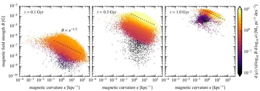
Figure 9: Emergence of the magnetic field and curvature in the galaxy centre ($r<1$ kpc). We show the mean density in the plane spanned by magnetic field strength $B$ and curvature $\kappa$ in our Milky Way-like halo (with mass $10^{12}~{}\mathrm{M}_{\odot}$ and concentration $c_{200}=7$). From left to right, the panels show the three characteristic phases of the magnetic dynamo: (i) exponential growth phase in the kinematic regime, (ii) growth of the magnetic coherence scale, and (iii) saturation phase of the magnetic dynamo. Starting with the kinematic phase through the growth phase of the magnetic coherence scale, there is a clear anticorrelation of $B^{2}$ and $\kappa$ visible at the largest density, which tightens up at the saturation phase, in particular at high curvature and gas density (which has a smaller dynamical timescale). We observe the expected correlation $B\propto\kappa^{-1/2}$ (Eq. 23) at various densities, which signals a superposition of different dynamo processes on different length and time scales characterised by different densities.

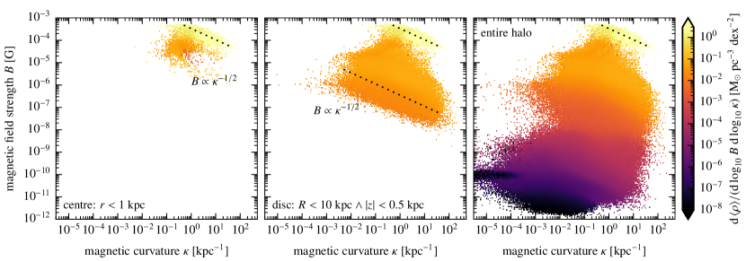
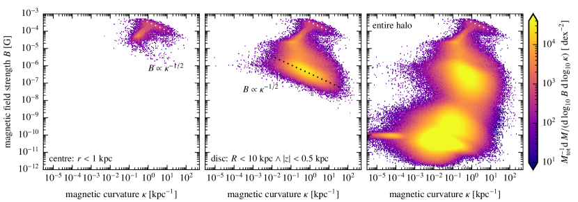
Figure 10: Separating different dynamo processes by spatial cuts for the saturated dynamo regime at 1 Gyr in our Milky Way-like halo (of mass $10^{12}~{}\mathrm{M}_{\odot}$ and concentration $c_{200}=7$). The top panels show the mean density in the plane spanned by magnetic field strength $B$ and curvature $\kappa$ while the bottom panels show the mass-weighted probability density. From left to right, we show the central sphere of radius 1 kpc (left), the disc region (middle) and the entire halo (right). This clearly demonstrates that while there is a complex superposition of different dynamo processes in the entire halo, these can be deconstructed by applying spatial cuts and restricting to a narrow range in mean density, which mirrors the behaviour of a small-scale dynamo in incompressible, homogeneous turbulent boxes (Schekochihin et al., 2004).

While the power spectrum is well suited for analysing the physical scales of magnetic field growth, it is not optimised for exploring the associated forces and to fully characterise the small-scale dynamo during galaxy formation. Thus, to complement our power-spectrum analysis, we turn to the Lorentz force density, which reads in terms of B in the MHD approximation:

$$\textbf{{f}}_{\mathrm{L}}=\frac{1}{c}\,\textbf{{j}}\bm{\times}\textbf{{B}}=\frac{1}{4\uppi}\left(\bm{\nabla}\bm{\times}\textbf{{B}}\right)\bm{\times}\textbf{{B}}=\frac{1}{4\uppi}\left(\textbf{{B}}\bm{\cdot}\bm{\nabla}\right)\textbf{{B}}-\frac{1}{8\uppi}\bm{\nabla}B^{2},$$ (21)

where the two terms on the right-hand side are often (erroneously) attributed to the magnetic curvature and pressure forces, respectively. In order to fully separate the effects of magnetic curvature and pressure – which are mixed up in this representation – we write $\textbf{{B}}=B\textbf{{b}}$, where b is the unit vector in the direction of B and obtain (Spruit, 2013)

$$\textbf{{f}}_{\mathrm{L}} =\frac{B^{2}}{4\uppi}\left(\textbf{{b}}\bm{\cdot}\bm{\nabla}\right)\textbf{{b}}+\frac{1}{8\uppi}\textbf{{b}}(\textbf{{b}}\bm{\cdot}\bm{\nabla})B^{2}-\frac{1}{8\uppi}\bm{\nabla}B^{2}$$

$$=\frac{B^{2}}{4\uppi}\left(\textbf{{b}}\bm{\cdot}\bm{\nabla}\right)\textbf{{b}}-\frac{1}{8\uppi}\bm{\nabla}_{\perp}B^{2}\equiv\textbf{{f}}_{\mathrm{c}}+\textbf{{f}}_{\mathrm{p}},$$ (22)

where we define the gradient perpendicular to the magnetic field lines, $\bm{\nabla}_{\perp}=(\bm{\mathsf{1}}-\textbf{{b}}\textbf{{b}})\bm{\cdot}\bm{\nabla}$. The second term, $\textbf{{f}}_{\mathrm{p}}$, acts like a pressure force perpendicular to the magnetic field lines and the first term, $\textbf{{f}}_{\mathrm{c}}$, is the magnetic curvature force that also acts in a plane orthogonal to the field line. To see this, we locally identify a curved field line with its curvature circle so that we can locally define an azimuthally directed field $\textbf{{B}}=B\textbf{{e}}_{\varphi}$ in cylindrical coordinates $(R,\varphi,z)$. Hence, in this case we obtain $(\textbf{{b}}\bm{\cdot}\bm{\nabla})\textbf{{b}}=(\textbf{{e}}_{\varphi}\bm{\cdot}\bm{\nabla})\textbf{{e}}_{\varphi}=-\textbf{{e}}_{R}/R$ so that the curvature force always points towards the centre of the curvature circle and aims to reduce the curvature by pulling the field line straight with a force that is the greater the smaller the curvature radius is.

Hence, it is advisable to define a magnetic curvature via

$$\bm{\kappa}\equiv(\textbf{{b}}\bm{\cdot}\bm{\nabla})\textbf{{b}}=\frac{\left(\bm{\mathsf{1}}-\textbf{{b}}\textbf{{b}}\right)\bm{\cdot}(\textbf{{B}}\bm{\cdot}\bm{\nabla})\,\textbf{{B}}}{B^{2}}=\frac{4\uppi\,\textbf{{f}}_{\mathrm{c}}}{B^{2}},$$ (23)

which immediately defines the curvature radius via

$$R_{\mathrm{c}}\equiv\frac{1}{\kappa}=\frac{1}{|\bm{\kappa}|}=\frac{1}{|(\textbf{{b}}\bm{\cdot}\bm{\nabla})\textbf{{b}}|}.$$ (24)

Equation (23) may seem to suggest that large curvature forces $f_{\mathrm{c}}=|\textbf{{f}}_{\mathrm{c}}|$ and small magnetic field strengths imply a large magnetic curvature. However, idealised simulations of incompressible, driven MHD turbulence show that in the regime of high curvature, $\kappa$ is not strongly correlated with a large curvature force but instead with a small value of the magnetic field strength while small magnetic curvature is correlated with a low level of curvature force (see figure 8 of Yang et al., 2019). Hence, the anticorrelation between $B^{2}$ and $\kappa$ is a consequence of the curvature force normal to the magnetic field line. A large curvature force rapidly straightens out any curved field line, which apparently precludes the possibility of a joint presence of a high curvature and a large magnetic field. Heuristically, this means that a strong magnetic field resists bending.

Most importantly, a magnetised plasma that does not experience any driving will evolve into a state that minimises magnetic tension and curvature (of course subject to the magnetic helicity constraint). Hence, the continued presence of magnetic curvature requires an active process such as a small-scale dynamo to build up and maintain a high level of magnetic curvature. In the following, we will study the emergence of magnetic curvature and its correlation properties with field strength and curvature force during galaxy assembly and growth, aiming at characterising the processes growing magnetic fields and whether this is consistent with a single or even multiple small-scale dynamos.

Figure 9 shows the correlation of $B$ and $\kappa$ in the galaxy centre ($r<1$ kpc), colour coded by the mean density in the pixels. At constant density, there is the expected correlation $B\propto\kappa^{-1/2}$ (Eq. 23) at high curvature, which is consistent with a small-scale dynamo (Schekochihin et al., 2004). The correlation weakens toward low curvature where the curvature force $f_{\mathrm{c}}$ starts to correlate with $\kappa$. We verified that there is no strong correlation of $f_{\mathrm{c}}$ and $\kappa$ at high curvature, which confirms the finding of Yang et al. (2019) who performed simulations of incompressible, driven MHD turbulence.

In contrast to those simplified setups, we demonstrate the emergence of this anticorrelation of $B^{2}$ and $\kappa$ at various densities in Fig. 9, suggesting a superposition of multiple small-scale dynamo modes. At the beginning, there is one small-scale dynamo mode growing the magnetic field in the centre (possibly associated with turbulence driven by the accretion shock). As this dynamo saturates the field in the centre at around 150 Myr (Fig. 4), other (small-scale) dynamo modes are excited at lower densities (in the central region but also in the disc and halo) that grow the magnetic field simultaneously to the saturated inner dynamo, however at a reduced rate. Those dynamos are likely driven by turbulence that has been injected by Kelvin-Helmholtz surface and body modes that are excited by the supersonically rotating cool galactic disc with respect to the hot halo gas.

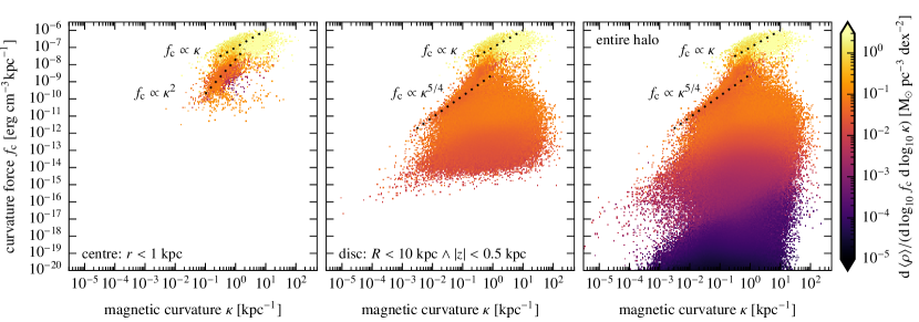
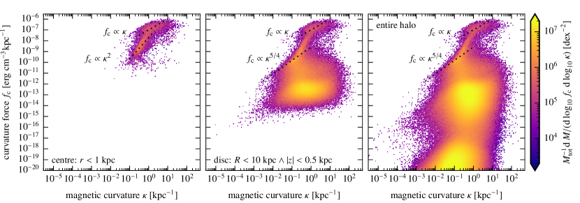
Figure 11: Correlation of the curvature force density $f_{\mathrm{c}}$ with curvature strength $\kappa$. The top panels show the mean density in the $f_{\mathrm{c}}$–$\kappa$ plane while the bottom panels show the mass-weighted probability density. From left to right, we show the central sphere of radius 1 kpc (left), the disc region (middle) and the entire halo (right). While there is little correlation at high curvature, the correlation at constant density tightens at intermediate curvature $\kappa\sim 1~{}\mathrm{kpc}^{-1}$ and shows the expected scaling $f_{\mathrm{c}}\propto\kappa$ (Eq. 23). The steepening of this correlation to $f_{\mathrm{c}}\propto\kappa^{2}$ at lower curvature in the central region suggests a non-trivial $B(\kappa)$ scaling.

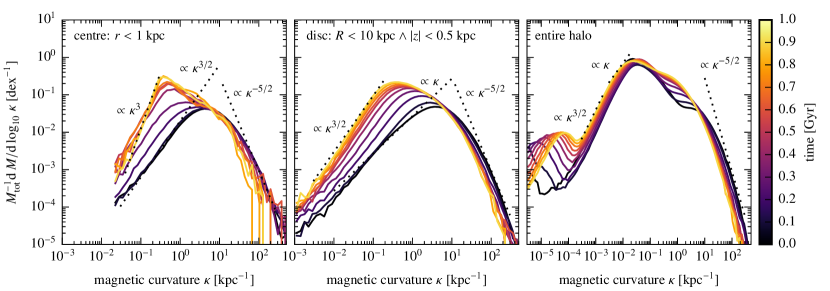
Figure 12: Mass-weighted probability density of magnetic curvature for the central 1 kpc (left), the disc region (middle) and the entire halo (right). In all cases (and excluding very small curvatures $\kappa<10^{-3}~{}\mathrm{kpc}^{-1}$), we see that after the initial exponential growth phase (i.e., for $t\gtrsim 150$ Myr), there is a growth phase of the magnetic coherence scale, which thus reduces the magnetic curvature scale. The asymptotic behaviour is consistent with turbulent MHD simulations by Yang et al. (2019). Note the extended abscissa in the rightmost panel for the entire halo.

This picture becomes even richer if we increase the size of the analysing region from the central region to the full disc (with a disc radius $R<10$ kpc and vertical height $|z|<0.5$ kpc) and the entire halo in Fig. 10. There, we show the mean density (top panels) and the mass-weighted probability density (bottom panels) in the $B$–$\kappa$ plane at the saturation phase of the magnetic dynamo in the centre ($t=1$ Gyr). The disc and halo regions show a larger range in densities and hence, dynamical time-scales, which shows a complex superposition of different dynamo processes. Focusing on the disc region (top middle panel), there are at least three different dynamo processes operating, each separated by the characteristic density: the upper sequence corresponds to the small-scale dynamo in the central region while the lower branches are related to dynamo processes in the outer disc.

Restricting to a narrow range in mean density, we see the expected correlation $B\propto\kappa^{-1/2}$ at high curvatures, respectively, which is consistent with MHD simulations of the small-scale dynamo in incompressible and homogeneous turbulence of high magnetic Prandtl number and low Reynolds number (Schekochihin et al., 2004). At lower curvature, the correlations substantially weaken, which is also seen in complementary MHD simulations of high Reynolds number and a magnetic Prandtl number of unity (see figure 8 of Yang et al., 2019).

Figure 11 shows the correlation of the magnitude of the curvature force $f_{\mathrm{c}}$ with the curvature $\kappa$: at intermediate magnetic curvature $\kappa\sim 1~{}\mathrm{kpc}^{-1}$, we observe a correlation of $\kappa$ and $f_{\mathrm{c}}$. This linear correlation steepens toward lower curvature to $f_{\mathrm{c}}\propto\kappa^{2}$ in the centre at the lowest curvature, which is a consequence of the linear correlation $B^{2}\propto\kappa$ in Fig. 10 and likely related to a compressible MHD effect. At lower values of the curvature force density $f_{\mathrm{c}}\lesssim 10^{-10}~{}\mathrm{erg~{}cm}^{-3}~{}\mathrm{kpc}^{-1}$ (in the disc region and the entire halo), there is little correlation so that the main diagnostic of the dynamo is indeed the anticorrelation of $\kappa$ and $B^{2}$ as derived in Eq. (23) and realised in our simulations at constant density (Figs. 9 and 10).

There have been analytical derivations of the probability density of $\kappa$ (Schekochihin et al., 2001, 2004; Yang et al., 2019), which we would like to confront to our simulations. Figure 12 shows the time evolution of the mass-weighted probability density of $\kappa$ for different spatial regions: the central sphere of radius 1 kpc, the disc region and the entire halo (from left to right). After the initial exponential growth phase for $t\gtrsim 150$ Myr and excluding very small curvatures $\kappa<10^{-3}~{}\mathrm{kpc}^{-1}$, the main effect is a shift of the peak of the distribution to smaller values of $\kappa$ or equivalently to larger curvature radii. This is the signature of a small-scale dynamo that is characterised by continuous growth of magnetic power on large scales until saturation at the corresponding larger kinetic turbulent energy, which increases the magnetic coherence scale with time. We also observe a change in the asymptotic power-law slopes and interesting structures in the probability density of the entire halo.

In order to quantify this behaviour, we note that the three spatial components of the magnetic field fluctuations are independent (subject to the $\bm{\nabla}\bm{\cdot}\textbf{{B}}=0$ constraint) and thus obey quasi-Gaussian distributions. Hence, the random variable $x=B^{2}=B_{x}^{2}+B_{y}^{2}+B_{z}^{2}$ follows a $\chi^{2}$ distribution with $k=3$ degrees of freedom,

$$f_{k}(x)=\frac{x^{k/2-1}\mathrm{e}^{-x/2}}{2^{k/2}\Gamma(k/2)},\quad x>0,$$ (25)

and $f_{k}(x)=0$ otherwise. $\Gamma(k)$ denotes the gamma function. We can thus derive the asymptotic limit $\kappa\to\infty$ of the probability density of $\kappa$ by using a Taylor expansion in the limit of $B\to 0$ (Yang et al., 2019):

$$f(\kappa)\mathrm{d}\kappa=f_{3}(B^{2})\left|\frac{\mathrm{d}B^{2}}{\mathrm{d}\kappa}\right|\mathrm{d}\kappa\to\frac{(4\uppi f_{\mathrm{c}})^{3/2}}{\sqrt{2\uppi}}\,\kappa^{-5/2}\mathrm{d}\kappa.$$ (26)

Using the fact that in the regime of large curvature, $\kappa$ is not strongly correlated with the curvature force (see Fig. 11), we obtain the scaling of $f(\kappa\to\infty)\propto\kappa^{-5/2}$ for all analysed regions in Fig. 12, which agrees very well with the theoretical expectation of Eq. (26) in the limit $\kappa\to\infty$.

In order to derive the asymptotic limit $\kappa\to 0$ of the probability density of $\kappa$, we note that the curvature force is confined to a plane orthogonal to B. We can thus assume that $f_{\mathrm{c}}^{2}$ is $\chi^{2}$ distributed, with two degrees of freedom and use a Taylor expansion in the limit $f_{\mathrm{c}}\to 0$:

$$f(\kappa)\mathrm{d}\kappa=f_{2}(f_{\mathrm{c}}^{2})\left|\frac{\mathrm{d}f_{\mathrm{c}}^{2}}{\mathrm{d}\kappa}\right|\mathrm{d}\kappa\to\left(\frac{B^{2}}{4\uppi}\right)^{2}\,\kappa\mathrm{d}\kappa.$$ (27)

Idealised simulations of incompressible, driven MHD turbulence show that in the regime of small magnetic curvature ($\kappa\to 0$), the curvature and magnetic field strength are uncorrelated, implying $f(\kappa\to 0)\propto\kappa$ (Yang et al., 2019).

By contrast, in Figs. 10 and 11 we observe a superposition of various magnetic dynamos as well as correlations of curvature and magnetic field strength in the regime of lower curvature. Those result from adiabatic compression and/or pressure forces and gravity that can modify the behaviour of $f(\kappa)$ in interesting ways. Hence, projecting the two-dimensional probability density $f(\kappa,B)$ along $B$ (see Fig. 10) results in several bumps in $f(\kappa)$ as shown in Fig. 12. Those result from different dynamo processes (with the exception of the left-most bump of $f(\kappa)$ for the entire halo, which arises from the slightly modified initial conditions). During the exponential growth phase at the centre ($t\lesssim 150$ Myr), we observe a correlation of $f_{\mathrm{c}}\propto\kappa^{5/4}$ or equivalently $B^{2}\propto\kappa^{1/2}$ at small values of $\kappa$, which results in a steeper slope of $f(\kappa\to 0)\propto\kappa^{3/2}$. This limiting behaviour is also observed at 1 Gyr in our disc region and our entire halo. During the saturation phase of the magnetic dynamo at the centre ($t=1$ Gyr), we observe a stronger correlation of $f_{\mathrm{c}}\propto\kappa^{2}$ or equivalently $B^{2}\propto\kappa$, which results in a steeper slope of $f(\kappa\to 0)\propto\kappa^{3}$.

We conclude that the high-curvature limit of our simulations agrees with theoretical predictions of the small-scale dynamo in incompressible simulations of turbulence of high Reynolds number (Yang et al., 2019) while we obtain different scalings in comparison to simulations in the subviscous range of high magnetic Prandtl numbers (Schekochihin et al., 2004) who base their mathematical descriptions on studies of the time evolution of curvature in line and surface elements for a simple model turbulence (Drummond & Muench, 1991). We show that gravitational collapse and the inside-out formation of a galactic disc excite a superposition of different small-scale dynamo modes. In consequence, in the limiting regime at low curvature the probability density shows a complex scaling behaviour, which is subject to a compressibly modified magnetic field. This is a direct consequence of the more complex velocity field in our simulation that is shaped by the gravitational collapse, CRs and ISM physics, which imprint more structure in the magnetic field. Contrarily, the velocity field in turbulent homogeneous boxes is randomly driven on large scales so that the velocity field is initially uncorrelated. Any structure in the velocity and magnetic field in those idealised boxes is thus generated by a small-scale dynamo while it is additionally shaped by compressible motions, gravity and ISM physics in our galaxy simulations.

4 FIR–radio correlation

We now analyse the radio synchrotron emission and start the discussion with the global FRC and sources of scatter. To understand this correlation we will show an analytical calculation of the FRC and analyse individual maps and profiles of the radio emission and other quantities of our simulated galaxies, which help in scrutinising whether our simulations reproduce the local FRC.

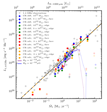
Figure 13: Correlation between the radio luminosity $L_{1.4\,\mathrm{GHz}}$ and FIR luminosity $L_{\mathrm{FIR}}$ (top axis) or SFR (bottom axis) of star-forming galaxies. The observed galaxies (open circles, Bell, 2003) exhibit a best-fit relation (orange dashed) that is slightly steeper than the linear calorimetric relation (Eq. 29) and perfectly agrees with our analytically derived FRC (black solid, Eq. 40). We overplot the emission of our simulated galaxies that only account for advective CR transport (‘CR adv’, red and orange) and simulations in which we additionally follow anisotropic CR diffusion (‘CR diff’, blue and green). Semi-transparent symbols correspond to a phase of a growing magnetic dynamo whereas fully-coloured symbols characterise the stages of a saturated dynamo and fall on the observed relation. The solid blue (purple) lines delineate time evolution tracks of simulated galaxies ($3\times 10^{11}~{}\mathrm{M}_{\odot}$, face-on projection) with initial magnetic field strength $10^{-10}~{}\upmu$G ($10^{-12}~{}\upmu$G). We contrast edge-on projections (orange and green) to face-on views (red and blue), which mostly exhibit a higher luminosity because the entire toroidal disc field contributes to the synchrotron intensity.

4.1 Global FIR–radio correlation

The FIR luminosity ($L_{\mathrm{FIR}}$, $8-1000~{}\upmu$m) is related to the SFR, $\dot{M}_{\star}$, of spiral galaxies (Schmidt, 1959; Kennicutt, 1998b, a),

$$\frac{\dot{M}_{\star}}{\mathrm{M}_{\odot}~{}\mathrm{yr}^{-1}}=\epsilon\,1.7\times 10^{-10}\,\frac{L_{\mathrm{FIR}}}{\mathrm{L}_{\odot}}.$$ (28)

This conversion assumes that thermal dust emission calorimetrically traces the emission of young stars, and the factor $\epsilon=0.79$ derives from the Chabrier (2003) initial mass function.

In Fig. 13 we correlate the total specific radio synchrotron luminosity $L_{1.4\,\mathrm{GHz}}$ with the SFR of our differently-sized galaxies at various times, which also correspond to different FIR luminosities as is shown at the top horizontal axis. We select simulation times such that we sample the SFR in logarithmically-equidistant steps of one e-folding, starting with the maximum during the initial starburst. Our simulations in the saturated small-scale dynamo regime (shown with the fully-coloured data points) match the observed FRC extremely well.

Observational data (as compiled by Bell, 2003) exhibit a best-fitting relation that is slightly steeper than the linear calorimetric relation,

$$L_{1.4\,\mathrm{GHz}}=\tilde{L}_{0}\left(\frac{L_{\mathrm{FIR}}}{10^{10}\mathrm{L}_{\odot}}\right)^{\alpha_{\mathrm{FRC}}},$$ (29)

where $\tilde{L}_{0}=2.26\times{10}^{28}\,\mathrm{erg~{}s}^{-1}~{}\mathrm{Hz}^{-1}$ and $\alpha_{\mathrm{FRC}}=1.055$. Combining Eqs. (28) and (29) yields

$$\frac{L_{1.4\,\mathrm{GHz}}}{\dot{M}_{\star}}=\frac{L_{0}}{\mathrm{M}_{\odot}~{}\mathrm{yr}^{-1}}\left(\frac{\dot{M}_{\star}}{\mathrm{M}_{\odot}~{}\mathrm{yr}^{-1}}\right)^{\alpha_{\mathrm{FRC}}-1},$$ (30)

where $L_{0}=1.68\times{10}^{28}\,\mathrm{erg~{}s}^{-1}~{}\mathrm{Hz}^{-1}$.

The purple and blue lines in Fig. 13 trace the time evolution of the SFR and synchrotron luminosity $L_{1.4\,\mathrm{GHz}}$ of a simulated galaxy ($3\times 10^{11}~{}\mathrm{M}_{\odot}$) with initial magnetic field strengths $B_{\mathrm{init}}=10^{-12}~{}\upmu$G and $10^{-10}~{}\upmu$G, respectively. During the kinematic phase of the dynamo, the model with the larger value of $B_{\mathrm{init}}$ grows faster and produces a larger radio luminosity. At the time of saturation, the tracks of simulations with different $B_{\mathrm{init}}$ start to converge, but retain memory of their different evolution and show radio luminosities that differ by a factor of up to two as a result of the stochasticity of the star formation process triggered by the different magnetic realisations of both models.

4.2 Analytics

To understand the reason for this success of matching the FRC, we will show that it is a necessary consequence of electron calorimetry, thus generalising the findings of Thompson et al. (2007) to also include primaries in addition to secondary electrons. First, we relate the CR proton luminosity, $L_{\mathrm{p}}$, to the SFR via

$$L_{\mathrm{p}}=\zeta_{\mathrm{SN}}\dot{M}_{\star}\frac{E_{\mathrm{SN}}}{M_{\star}}=5.5\times 10^{-4}\,\zeta_{\mathrm{SN},0.05}L_{\mathrm{FIR}},$$ (31)

where we used Eq. (28) to eliminate the SFR and $\zeta_{\mathrm{SN},0.05}=\zeta_{\mathrm{SN}}/0.05$ is the kinetic energy fraction of SNRs injected into CR protons (Pais et al., 2018). Assuming a Chabrier (2003) initial mass function and that stars with a mass of $8-40~{}\mathrm{M}_{\odot}$ explode as supernovae (while they directly collapse to a black hole above $40~{}\mathrm{M}_{\odot}$, Fryer, 1999), there is about one core-collapse supernova per $100~{}\mathrm{M}_{\odot}$ of newly formed stars. Thus, we obtain a canonical supernova energy release per unit stellar mass of $E_{\mathrm{SN}}/M_{\star}=10^{51}~{}\mathrm{erg}/(100~{}\mathrm{M}_{\odot})=1\times 10^{49}~{}\mathrm{erg}~{}\mathrm{M}_{\odot}^{-1}$. The total luminosity of primary and secondary electrons is given by

$$L_{\mathrm{e}}=\left(\zeta_{\mathrm{prim}}+\zeta_{\mathrm{sec}}\eta_{\mathrm{cal,p}}\right)L_{\mathrm{p}}=\zeta_{\mathrm{e}}L_{\mathrm{p}}\approx 0.27L_{\mathrm{p}},$$ (32)

where $\zeta_{\mathrm{prim}}\approx 0.09$ is the energy ratio of primary CR electrons and protons given by Eq. (6), $\zeta_{\mathrm{sec}}=\varepsilon_{\mathrm{sec}}/\varepsilon_{\mathrm{p}}\approx 0.25$ is the energy ratio of secondary CR electrons and protons (as we will show below), and $\eta_{\mathrm{cal,p}}=\Lambda_{\mathrm{hadr}}/(\Lambda_{\mathrm{hadr}}+\Lambda_{\mathrm{Coul}})\approx 0.73$ is the calorimetric fraction of CR proton energy that cools via hadronic interactions as supposed to Coulomb interactions (where $\Lambda_{\mathrm{hadr}}$ and $\Lambda_{\mathrm{Coul}}$ are the hadronic and Coulomb cooling rates, Pfrommer et al., 2017a). In hadronic interactions, approximately 2/3 of the CR proton energy is channeled into charged pions, which subsequently decay into high-energy neutrinos and electron-positron pairs so that the pairs receive 1/4 of the pion energy (Schlickeiser, 2002). To arrive at the result for $\zeta_{\mathrm{sec}}$, we also account for the nuclear enhancement factor of 1.4 to 1.6, that accounts for heavier nuclei in the composition of CRs and the ISM (Białłas et al., 1976; Stephens & Badhwar, 1981). In the following, we adopt $\zeta_{\mathrm{e}}=0.27$ and $\zeta_{\mathrm{SN}}=0.05$ as fiducial values and drop the explicit dependence on these variable in our calculation. In order to connect this bolometric electron luminosity to the spectral radio luminosity, we have to calculate the bolometric energy fraction emitted into the radio band. To this end, we write down the volume-integrated injected electron distribution (which we assume to be a simple power-law momentum distribution):

$$Q_{\mathrm{e}}(p_{\mathrm{e}})=\frac{\mathrm{d}N_{\mathrm{e}}}{\mathrm{d}p_{\mathrm{e}}\mathrm{d}t}=\int q_{\mathrm{e}}(p_{\mathrm{e}})\mathrm{d}V={\mathcal{C}}_{\mathrm{e}}p_{\mathrm{e}}^{-\alpha}\theta(p_{\mathrm{e}}-p_{\mathrm{min}}),$$ (33)

where $p_{\mathrm{min}}$ is the dimensionless low-momentum cutoff, ${\mathcal{C}}_{\mathrm{e}}$ is the normalization (in units of s^-1), and $\theta(p)$ denotes the Heaviside step function. The CR electron luminosity is given by

$$L_{\mathrm{e}} =\int_{0}^{\infty}Q_{\mathrm{e}}(p_{\mathrm{e}})\,T_{\mathrm{e}}(p_{\mathrm{e}})dp_{\mathrm{e}}=\frac{{\mathcal{C}}_{\mathrm{e}}\,m_{\mathrm{e}}c^{2}}{\alpha-1}$$ (34)

$$\quad\times\left[\frac{1}{2}\,{\mathcal{B}}_{\frac{1}{1+p_{\mathrm{min}}^{2}}}\left(\frac{\alpha-2}{2},\frac{3-\alpha}{2}\right)+p_{\mathrm{min}}^{1-\alpha}\left(\sqrt{1+p_{\mathrm{min}}^{2}}-1\right)\right],$$

$$\equiv{\mathcal{C}}_{\mathrm{e}}\,m_{\mathrm{e}}c^{2}A_{\mathrm{bol}}(p_{\mathrm{min}},\alpha)$$ (35)

where $T_{\mathrm{e}}(p_{\mathrm{e}})=\left(\sqrt{1+p_{\mathrm{e}}^{2}}-1\right)\,m_{\mathrm{e}}c^{2}$ is the kinetic electron energy, ${\mathcal{B}}_{y}(a,b)$ denotes the incomplete beta function (Abramowitz & Stegun, 1965), and we assume $\alpha>2$. The bolometric energy fraction $A_{\mathrm{bol}}(p_{\mathrm{min}},\alpha)^{-1}$ depends only weakly on $p_{\mathrm{min}}$ (provided that $p_{\mathrm{min}}\lesssim 1$) and enables us to rewrite the electron source distribution via

$$E_{\mathrm{e}}^{2}Q(E_{\mathrm{e}})\equiv\frac{E_{\mathrm{e}}\mathrm{d}N_{\mathrm{e}}}{\mathrm{d}\ln\gamma_{\mathrm{e}}\,\mathrm{d}t}\approx m_{\mathrm{e}}c^{2}{\mathcal{C}}_{\mathrm{e}}\gamma_{\mathrm{e}}^{2-\alpha}=\frac{L_{\mathrm{e}}}{A_{\mathrm{bol}}}\,\gamma_{\mathrm{e}}^{2-\alpha},$$ (36)

where $\gamma_{\mathrm{e}}$ is the electron Lorentz factor. In the second step, we adopted the electron distribution in the relativistic limit (Eq. 33), which is valid for synchrotron-emitting electrons. Assuming that the synchrotron cooling time of CR electrons is shorter than their escape times (Völk, 1989), we find an FRC of the form

$$\nu L_{\nu}(\mathrm{GHz}) =\frac{E_{\gamma}\mathrm{d}N_{\gamma}}{\mathrm{d}\ln\nu\,\mathrm{d}t}=\eta_{\mathrm{syn}}\,\frac{E_{\mathrm{e}}\mathrm{d}N_{\mathrm{e}}}{2\,\mathrm{d}\ln\gamma_{\mathrm{e}}\,\mathrm{d}t}\approx\frac{\eta_{\mathrm{syn}}}{2A_{\mathrm{bol}}}\,\gamma_{\mathrm{e}}^{2-\alpha}L_{\mathrm{e}}$$ (37)

$$\approx 8.36\times 10^{-7}\,\left(\frac{\eta_{\mathrm{syn}}}{0.30}\right)\,\left(\frac{\gamma_{\mathrm{e}}}{8.4\times 10^{3}}\right)^{2-\alpha}L_{\mathrm{FIR}},$$ (38)

where we have used Eqs. (31) and (32) in the last step. Here, $\mathrm{d}\ln\nu=2\,\mathrm{d}\ln\gamma_{\mathrm{e}}$ according to Eq. (9), $\eta_{\mathrm{syn}}$ denotes the calorimetric energy fraction of electrons that cool and radiate synchrotron emission, and we adopted in the last step $\alpha=2.2$, $p_{\mathrm{min}}=1$, and electrons with a Lorentz factor $\gamma_{\mathrm{e}}=8.4\times 10^{3}$ that emit 1.4 GHz synchrotron radiation in a magnetic field of $2.4~{}\upmu$G (see Eq. 9). In our models, $\eta_{\mathrm{syn}}$ ranges from 0.1 to 0.7 at SFRs $\dot{M}_{\star}\gtrsim 1~{}\mathrm{M}_{\odot}~{}\mathrm{yr}^{-1}$, with slightly smaller (larger) values realised in our ‘CR diff’ (‘CR adv’) models (Werhahn et al., 2021c). We note that the lowest values of $\eta_{\mathrm{syn}}$ in the ‘CR diff’ model are realised in our $10^{10}~{}\mathrm{M}_{\odot}$ halo and could become larger if we use an improved ISM model in cosmological simulations of dwarf galaxies with (i) star formation- and cosmic accretion-driven turbulence that helps to further grow the disc magnetic field as well as (ii) an improved CR transport model which delivers a realistic (spatially and temporally varying) CR diffusion coefficient in the self-confinement picture (Thomas & Pfrommer, 2019).

Interestingly, the factor $\gamma_{\mathrm{e}}^{2-\alpha}$ predicts a slightly super-linear FRC because of the different saturation values of the magnetic field strength with halo mass and SFR (see Fig. 1). In our ‘CR diff’ model, we find saturated magnetic field strengths of $[0.14,1.8,7,14]~{}\upmu$G for SFRs of $[0.01,0.4,5,30]~{}\mathrm{M}_{\odot}~{}\mathrm{yr}^{-1}$. This implies that the Lorentz factor of the electrons that emit 1.4 GHz synchrotron radiation of $\gamma_{\mathrm{e}}\approx[35,9.6,4.8,3.5]\times 10^{3}$ according to Eq. (9) which we fit in order to obtain a functional dependence of the 1.4 GHz synchrotron emitting Lorentz factor on the SFR,

$$\gamma_{\mathrm{e}}=8.4\times 10^{3}\,\left(\frac{\dot{M}_{\star}}{\mathrm{M}_{\odot}~{}\mathrm{yr}^{-1}}\right)^{-0.3}.$$ (39)

Using the Kennicutt (1998b) relation of Eq. (28) as well as Eq. (39), we can rewrite Eq. (38) and obtain the specific radio luminosity at 1.4 GHz,

$$L_{1.4\,\mathrm{GHz}}\approx~{} 1.7\times 10^{28}\,\left(\frac{\eta_{\mathrm{syn}}}{0.30}\right)\,\left(\frac{\dot{M}_{\star}}{\mathrm{M}_{\odot}~{}\mathrm{yr}^{-1}}\right)^{1.06}\mathrm{erg~{}s}^{-1}~{}\mathrm{Hz}^{-1},$$ (40)

where we adopted $\alpha=2.2$. In general, the power-law index in this correlation depends on the electron spectral index and reads $\alpha_{\mathrm{FRC}}=1+0.3(\alpha-2)$. This correlation coincides with the observed super-linear FRC by Bell (2003) which obeys the fitting relation of Eq. (30). Figure 13 shows a comparison of observed (orange dashed) and theoretical (black solid) mean FRC, which are nearly identical. Werhahn et al. (2021c) find that $\eta_{\mathrm{syn}}$ increases with time along the evolutionary path of a galaxy (for the $M_{200}\gtrsim 3\times 10^{11}~{}\mathrm{M}_{\odot}$ haloes), because of the decreasing gas densities (see Section 4.4) and hence the increasing cooling times of bremsstrahlung and Coulomb interactions. This implies that the galaxies evolve from the lower to the upper envelope of the FRC as their SFR decreases with time. There are several other processes that cause scatter in the FRC which we will analyse now.

4.3 Scatter of the global FIR–radio correlation

We identify three physical effects that contribute to the scatter in the FRC: (i) initial magnetic field strength in combination with stochasticity of the star formation process and intermittent galactic winds, which modulate the magnetic and CR energy as well as the resulting synchrotron luminosity in the inner regions that are affected by the wind, (ii) different halo masses and thus different specific SFRs at a given absolute SFR and (iii) the galactic inclination in combination with an anisotropic magnetic field distribution cause variations of the radio intensity.

1. At early times in the kinematic dynamo regime, when the magnetic field strength is still exponentially growing (transparently coloured points in Fig. 13), the galaxies fall short by orders of magnitude of the observed FRC. However, in the saturated dynamo regime the tracks of simulations with different $B_{\mathrm{init}}$ start to converge, but nevertheless retain memory of their different evolution. While the observed FRC of nearby galaxies (within 255 Mpc, Bell, 2003) probes this saturated dynamo regime, our simulations imply a residual scatter if galaxies had different seed magnetic fields at the formation time or a different formation history and magnetic dynamo efficiencies. This could potentially be caused by the stochasticity of the star formation process. On top of this average trend, we see an upwards deviation of the purple track in Fig. 13 at around 1.6 $\mathrm{M}_{\odot}~{}\mathrm{yr}^{-1}$. This is due to a drop in the wind speed, which retains more CRs and a larger magnetic energy in the central region, and as a result, temporarily boosts the radio synchrotron emissivity by a factor of two.

2. As the small-scale dynamo has saturated, the galaxies move largely along the observed relation toward smaller SFRs and radio luminosities with a tendency to move from the lower to the upper envelope of the observational scatter (see Fig. 13). There are two reasons for this behaviour after the starburst phase. First, as explained in Section 4.2, smaller SFRs imply smaller gas densities and smaller collisional loss rates so that the calorimetric energy fraction emitted via radio synchrotron increases (Werhahn et al., 2021c). Second, the decreasing gas accretion onto the disc and thus the decreasing SFRs also lowers the CR proton injection rate. By contrast, there appears to be a magnetic dynamo that counteracts this decreasing trend of the CR and thermal energy densities so that the magnetic energy density remains constant with time. Thus, the total synchrotron emissivity decreases less strongly than the SFR and a galaxy evolves from the lower towards the upper envelope of the FRC. Thus, these two effects combined predict that at a given SFR, less massive systems with high specific SFRs to populate the lower envelope of the FRC in comparison to more massive systems that are in a late evolutionary phase with small specific SFRs.

3. There is a third effect that contributes to the FRC scatter by a factor of up to two. In the saturated dynamo regime, the toroidal disc field dominates over the poloidal components by an order of magnitude (Pakmor et al., 2016c). Observing such a galaxy face-on maximises the available synchrotron intensity (since the toroidal field is transverse to the line-of-sight in this configuration), whereas the intensity drops by a factor of two for an edge-on geometry (since half the toroidal field is now aligned with the line-of-sight). Conversely, a strong outflow generates a field morphology with substantial poloidal components and reduces the factor in between face-on and edge-on geometries as can be seen by the reverse ordering of the red and orange data points in the $3\times 10^{11}~{}\mathrm{M}_{\odot}$ halo at an SFR of around $1.5~{}\mathrm{M}_{\odot}~{}\mathrm{yr}^{-1}$. Note that supernova-driven turbulence may change the global field topology in the spiral-arm regions in the disc to a preferred turbulent magnetic configuration instead of a dominant toroidal morphology, which would significantly weaken the described effect. However, observations of the polarised thermal dust emission in M82 find a dominant large-scale ordered potential field associated with the outflow (Lopez-Rodriguez et al., 2021) so that the described effect may be most important for ordered poloidal fields in galactic winds.

Finally, we find that galaxies in the model ‘CR diff’ (‘CR adv’) populate the lower (upper) envelope of the observed relation after they have entered the saturated dynamo regime (fully-coloured symbols). There are two effects that cause this behaviour. First, the CR energy density is larger in the ‘CR adv’ model at small galaxy masses (see Fig. 1). This also causes a separation of the FIR–gamma-ray correlation at low SFRs (Pfrommer et al., 2017b; Werhahn et al., 2021b). Second, we find that the outflows driven by anisotropically diffusing CRs quench the magnetic dynamo and increase its growth time in comparison to model ‘CR adv’ (similarly to the case of isotropic diffusion, which quenches the dynamo in comparison to the anisotropic diffusion case, Pakmor et al., 2016c). Hence, galaxies in model ‘CR adv’ reach the observational relation earlier and saturate at higher field strengths. The $10^{10}~{}\mathrm{M}_{\odot}$ halo in model ‘CR diff’ never reaches the FRC and peaks around $L_{1.4~{}\mathrm{GHz}}\approx 10^{24}~{}\mathrm{erg~{}s}^{-1}\mathrm{Hz}^{-1}$. Apparently, modelling CR diffusion with a constant diffusion coefficient $10^{28}~{}\mathrm{cm}^{2}~{}\mathrm{s}^{-1}$ removes the gas too fast from this low-mass disc so that the dynamo lags behind, suggesting a more subtle CR transport process in dwarfs. In summary, an increasing (constant) CR diffusion coefficient moves galaxies to the lower envelope of the simulated FRC.

A more realistic modelling of CR transport in the CR self-confinement picture leads to a superposition of advection, diffusion and streaming with a spatially and temporally varying effective diffusion coefficient (Jiang & Oh, 2018; Thomas & Pfrommer, 2019, 2022; Thomas et al., 2020; Thomas et al., 2021). Future work is needed to study whether there is a range of effective CR diffusion coefficients at a fixed SFR, which would imply a third source of scatter in the observed FRC by indirectly affecting the FRC through its influence on the magnetic dynamo. Interestingly, observational studies of the local FRC demonstrate that the radio emissivity depends on CR transport properties in different environments (Basu et al., 2012, 2017; Heesen et al., 2014; Heesen et al., 2019), although the level of agreement with simulations would have to be carefully studied in future work.

4.4 Radio morphology of discs and CR-driven outflows

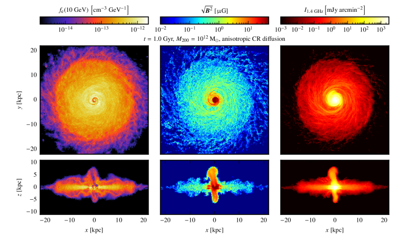
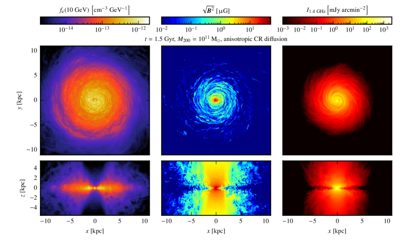
Figure 14: Properties of the gas disc in our Milky Way-mass galaxy at 1 Gyr ($M_{200}=10^{12}~{}\mathrm{M}_{\odot}$, $c_{200}=7$, top panels) and in our smaller galaxy at 1.5 Gyr ($M_{200}=10^{11}~{}\mathrm{M}_{\odot}$, $c_{200}=12$, bottom panels). The MHD simulations account for CR injection at SNRs, follow CR advection with the gas and anisotropic diffusion along magnetic fields relative to the gas. We show cross-sections in the mid-plane of the disc (face-on views) and vertical cut-planes through the centre (edge-on views) of the total (primary and secondary) CR electron spectral density at 10 GeV (left), total magnetic field strength (middle) and the total radio synchrotron brightness, $I_{\mathrm{1.4\,\mathrm{GHz}}}$ (right). The magnetically-loaded outflows are visible as bubbles in the Milky Way-mass galaxy and as an X-shaped radio morphology for the smaller galaxy (edge-on views on the right-hand side).

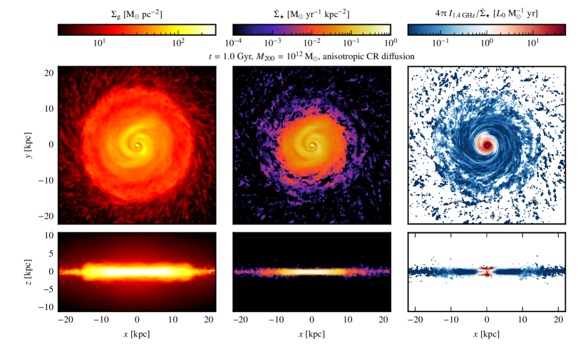
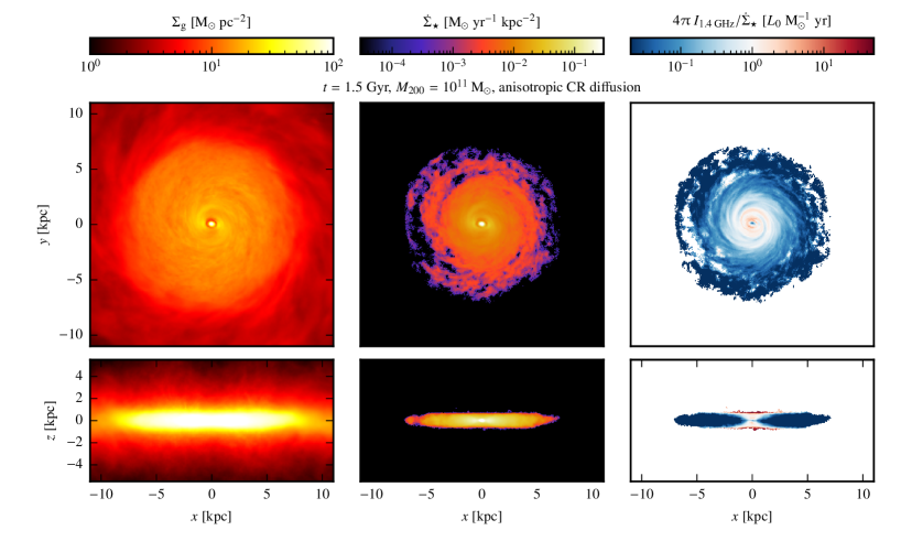
Figure 15: Shown are face-on and edge-on views of the surface mass density of gas (left), SFR surface density (middle) and the ratio of the radio synchrotron brightness-to-SFR surface density, $4\uppi\,I_{\mathrm{1.4\,GHz}}/\dot{\Sigma}_{\star}$ (right). Note that we scale this ratio to the mean radio flux $L_{0}$ of the observed FRC at an SFR of $1\,\mathrm{M}_{\odot}\,\mathrm{yr}^{-1}$ (Eq. 30) so that red (blue) colours indicate an excess (deficiency) in comparison to the observed FRC. We use the same simulation snapshots as in Fig. 14.

In Fig. 14, we show face-on and edge-on views of the total CR electron spectral density at 10 GeV and the magnetic field strength (left-hand and middle panels) for our galaxies with halo masses $10^{12}$ and $10^{11}~{}\mathrm{M}_{\odot}$. While the Milky Way-mass galaxy shows bubble-like CR-driven outflows, there are fast outflows in the smaller galaxy, which evacuate a bi-conical, X-shaped region in the circumgalactic medium (visible in yellow colours in the bottom-right panel of Fig. 14). In both galaxies, the outflows are strongly magnetised and and rich in CR electrons and protons (cf. Fig.1 in Pfrommer et al., 2017b, for the Milky Way-mass galaxy with halo mass $M_{200}=10^{12}~{}\mathrm{M}_{\odot}$ and concentration $c_{200}=7$). After the formation of the dense gas disc the CR pressure gradient is mostly vertically aligned so that it accelerates the ISM and drives outflows perpendicular to the stellar and gaseous discs. Thus, these CR-driven winds are an emergent phenomenon and the result of the outflows taking the path of least resistance away from the galaxies. Both galaxies show magnetic spiral arms which have counterparts in the surface gas density (cf. Figs. 14 and 15).

As we will show below, the magnetic dynamo grows slower at larger radii and we likely underestimate the dynamo growth at large galactocentric radii with our pressurised ISM (Springel & Hernquist, 2003), that neglects most of supernova-driven turbulence with the exception of our explicit injection of CR energy with an efficiency $\zeta_{\mathrm{SN}}=0.05$ and 0.1 of the canonical supernova energy. Correctly resolving the momentum and thermal energy input of supernova explosions that are clustered (Girichidis et al., 2016a) and maintain memory of their birthplaces at the junction of filaments (with sub-parsec widths, Arzoumanian et al., 2011; Schneider et al., 2012; Priestley & Whitworth, 2021; Whitworth et al., 2021) within molecular clouds is only possible for the mass resolution of a few solar masses in isolated stratified boxes at moderate (Milky Way-like) surface mass densities (Rathjen et al., 2021) or for dwarf galaxies (Gutcke et al., 2021). Only at this mass resolution, it is possible to form a multi-phase ISM with a volume-filling hot ($10^{7}$ K) phase and to identify a mean-field dynamo (Gent et al., 2013).

The total radio emission is shown in the right-hand panels of Fig. 14. The emission of the Milky Way-mass galaxy is dominated by the disc and a bright bulge that sources magnetically-loaded outflows, which are visible as faint bubbles. On the contrary, the disc is almost invisible in the smaller galaxy at $1.5$ Gyr, which shows instead an X-shaped radio morphology in the outflow region that arises because of the overlap of the cylindrical outflow geometry that is mirrored in the magnetic field distribution and the conical cavities in the CR electron spectrum.

In Fig. 15, we compare face-on and edge-on views of the gas surface mass density and the SFR surface density (left-hand and middle panels). The additional CR pressure support inflates the gas discs and thus enhances the gas density above and below the discs. By contrast, only gas in a thin disc exceeds the critical gas density necessary to form stars (Kennicutt, 1998b). The larger centrifugal support in the Milky Way-mass galaxy in comparison to the smaller galaxy implies a thinner stellar disc (see the discussion in Section 3.1). Note that the edge-on projection of the gas density yields a maximum gas surface mass density of $\Sigma_{\mathrm{g}}\approx 3\times 10^{9}\,\mathrm{M}_{\odot}~{}\mathrm{kpc}^{-2}$, a factor of 30 larger than the maximum value of the face-on projection. This exemplifies the strong dependence of $\Sigma_{\mathrm{g}}$ on galactic inclination in all but the very compact, ultra-luminous infrared galaxies and suggests the choice of a parametrization that is independent of inclination (such as the SFR) for an independent variable to be correlated with the gamma-ray or radio emission. We will return to the right-hand panels of Fig. 15 in Section 4.5.

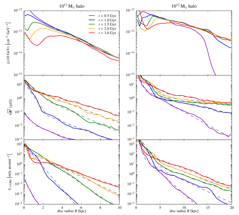
Figure 16: Radial disc profiles of our small galaxy ($M_{200}=10^{11}~{}\mathrm{M}_{\odot}$, $c_{200}=12$, left column) and our Milky Way-mass galaxy ($M_{200}=10^{12}~{}\mathrm{M}_{\odot}$, $c_{200}=7$, right column) at different times (as indicated in the legend). We show volume-averaged profiles of the total (primary and secondary) CR electron spectral density at 10 GeV (top), root mean square magnetic field strength (middle), both averaged in a disc of total height 1 kpc, and the total face-on radio synchrotron brightness at $\nu=1.4$ GHz (bottom). The profiles show a CR electron spectral density that decreases in radius and time, which is a consequence of the decreasing SFR, a growing magnetic field in the outer disc with time, which together imply increasing synchrotron surface brightness profiles with time. The radial profiles of magnetic field strength and synchrotron emission are well fit by joint exponentials (dashed lines, Eqs. 41 and 42).

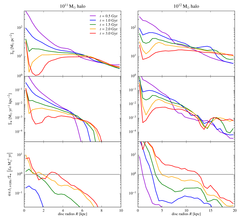
Figure 17: Radial disc profiles of the surface mass density of gas (top), SFR surface density (middle) and the ratio of the radio synchrotron brightness-to-SFR surface density, $4\uppi\,I_{\mathrm{1.4\,GHz}}/\dot{\Sigma}_{\star}$ (bottom), scaled to the mean radio flux $L_{0}$ of the observed FRC at an SFR of $1\,\mathrm{M}_{\odot}\,\mathrm{yr}^{-1}$ (Eq. 30). We use the same simulations and snapshots as in Fig. 16.

Table 2: Fitting parameters for the profiles of the disc magnetic field and the specific synchrotron intensity as a function of disc radius $R$. The joint exponential profiles in Eqs. (41) and (42) are characterised by a normalization ($B_{0}$ and $I_{0}$), a transition radius $r_{\mathrm{tr}}$, and the scale radii of the inner and outer exponentials, $r_{0}$ and $r_{1}$.

		magnetic profile $B(R)$				synchrotron intensity $I_{1.4\,\mathrm{GHz}}(R)$
halo	simulation time	$B_{0}$	$r_{\mathrm{tr}}$	$r_{0}$	$r_{1}$	$I_{0}$	$r_{\mathrm{tr}}$	$r_{0}$	$r_{1}$
|[$\mathrm{M}_{\odot}$]	[Gyr]	[$\upmu$G]	[kpc]	[kpc]	[kpc]	[mJy arcmin-2]	[kpc]	[kpc]	[kpc]
$10^{11}$	0.5	0.1	1.3	0.6	1.6	$2.9\times 10^{-2}$	1.9	0.3	0.3
$10^{11}$	1.0	15.5	2.5	0.4	1.6	$7.4\times 10^{1}$	0.1	1.9	0.4
$10^{11}$	1.5	24.5	2.7	0.7	1.4	$9.6\times 10^{1}$	1.8	0.7	0.7
$10^{11}$	2.0	24.0	0.9	0.5	1.7	$1.2\times 10^{2}$	0.4	0.2	1.0
$10^{11}$	3.0	20.4	1.1	0.6	2.1	$1.3\times 10^{2}$	0.8	0.2	1.4
$10^{12}$	0.5	137.3	1.9	0.5	2.3	$2.9\times 10^{4}$	1.7	0.3	1.0
$10^{12}$	1.0	120.9	4.5	1.0	5.9	$2.2\times 10^{4}$	4.2	0.5	1.9
$10^{12}$	1.5	109.4	5.7	1.2	13.4	$1.3\times 10^{4}$	5.0	0.6	2.5
$10^{12}$	2.0	74.2	6.5	1.6	11.5	$2.9\times 10^{3}$	5.7	1.0	2.4
$10^{12}$	3.0	37.6	6.5	2.3	7.9	$1.1\times 10^{4}$	1.8	0.4	2.4

To study the emergence of magnetic fields and synchrotron emission, we show average radial profiles of the CR electron spectral density $f_{\mathrm{e}}$ at 10 GeV, the magnetic field strength $B$, and the synchrotron intensity at different times in Fig. 16 for our two haloes of $10^{11}$ and $10^{12}~{}\mathrm{M}_{\odot}$. The initial gravitationally driven collapse of gas implies large central gas densities that ensues a vigorous starburst, as can be inferred from the average radial profiles of the surface mass density of gas $\Sigma_{\mathrm{g}}$ and SFR surface density $\dot{\Sigma}_{\star}$ at different times in Fig. 17. The CR electron spectrum mirrors this behaviour of the gas density and decreases at the centre while it remain nearly constant at larger radii. By contrast, the magnetic field strength grows with time in the outer disc. The growth rate is faster in the $10^{12}~{}\mathrm{M}_{\odot}$ halo in comparison to the smaller halo. The synchrotron emissivity mirrors the behavior of $B$.

The radial profile of the disc magnetic field can be well fit with two joint exponentials (Pakmor et al., 2017) that describe $B$ in two regions separated by a transition radius $r_{\mathrm{tr}}$, i.e., a four-parameter fit defined by

$$B(R)=\left\{\begin{array}[]{ll}B_{0}\mathrm{e}^{-R/r_{0}},&\mathrm{if}~{}~{}R<r_{\mathrm{tr}},\\ B_{0}\mathrm{e}^{-r_{\mathrm{tr}}/r_{0}-(R-r_{\mathrm{tr}})/r_{1}},&\mathrm{if}~{}~{}R\geq{r_{\mathrm{tr}}}.\end{array}\right.$$ (41)

Here, $B_{0}$ is the central field strength, $r_{0}$ and $r_{1}$ are the scale radii of the inner and outer exponentials. This functional form is well developed after the dynamo has saturated (even before outflows are launched) and suggests that two different amplification processes are responsible for growing magnetic fields in the corresponding regions. In our Milky Way-sized galaxy, the transition radius $r_{\mathrm{tr}}$ grows with time, while we only observe this behaviour at initial times (for $t\lesssim 1.5$ Gyr) in the $10^{11}~{}\mathrm{M}_{\odot}$ halo. Not surprisingly, the radial profile of the specific synchrotron intensity can also be well described by a joint exponential profile,

$$I_{\nu}(R)=\left\{\begin{array}[]{ll}I_{0}\mathrm{e}^{-R/r_{0}},&\mathrm{if}~{}~{}R<r_{\mathrm{tr}},\\ I_{0}\mathrm{e}^{-r_{\mathrm{tr}}/r_{0}-(R-r_{\mathrm{tr}})/r_{1}},&\mathrm{if}~{}~{}R\geq{r_{\mathrm{tr}}}.\end{array}\right.$$ (42)

where $I_{0}$ is the central synchrotron intensity and the other parameters have the same meaning as in Eq. (41). In contrast to the magnetic profile, the transition radius $r_{\mathrm{tr}}$ of the synchrotron profile shows a non-monotonic behaviour with time because the CR electron spectrum $f_{\mathrm{e}}$ obeys an opposite trend with time in comparison to $B$, i.e., the central normalisation of $f_{\mathrm{e}}$ decreases with time. We summarise all fitting parameters in Table 2.

4.5 Local FIR–radio correlation

In order to evaluate whether the FRC also holds on smaller scales within our galaxies, we need to first look at the limits of our ISM subgrid-scale model. In this model, star-forming gas is treated as a two phase medium of cold clouds embedded in an ambient hot medium, which is treated with an effective equation of state of a pressurised ISM and does not explicitly model molecular clouds. Hence, we show maps and profiles of the ratio of the radio synchrotron brightness-to-SFR surface density, $4\uppi\,I_{\mathrm{1.4\,GHz}}/\dot{\Sigma}_{\star}$ (right-hand panels of Fig. 15 and bottom panels of Fig. 17). We scale the radio emission to the mean radio flux $L_{0}$ of the observed FRC at a fiducial SFR of $\dot{M}_{\star\,0}=1\,\mathrm{M}_{\odot}\,\mathrm{yr}^{-1}$ (Eq. 30). Hence, we expect a ratio of order unity at this fiducial SFR and slightly larger (smaller) values at larger (smaller) SFRs due to the non-linearity of the FRC with an FRC slope of $\alpha=1.055$ (Eq. 29, Bell 2003) or $\alpha=1.11$ in a larger catalogue of 9,500 low-redshift galaxies (Molnár et al., 2021). Thus, a 100 times larger (smaller) SFR implies a 65 per cent increase (decrease) relative to the fiducial FRC ratio $L_{0}/\dot{M}_{\star\,0}$.

After saturation of the dynamo in our $10^{11}~{}\mathrm{M}_{\odot}$ halo, we observe the central few kpc to obey the local FRC. The centre of this galaxy shows an excess of the local FRC ratio that mimics the observed complex behavior with local extrema corresponding to various galactic structures, such as highly star-forming spiral arms emphasizing the strong environmental dependence of the thermal and non-thermal radio emission (e.g., in M51, see Dumas et al., 2011). These observations show a sub-linear FRC in the low-density interarm and outer region and super-linear behaviour in the central 3.5 kpc which is also visible in the bottom right-hand panel of Fig. 15. By contrast, the $10^{12}~{}\mathrm{M}_{\odot}$ halo severely exceeds the local FRC in the centre while it agrees within the scatter at late times and radii $5\lesssim R/\mathrm{kpc}\lesssim 12$. This could either signal a shortcoming in our star-formation and/or radio modelling or provide a hint that the centres of starbursts exceed the FRC by a substantial amount.

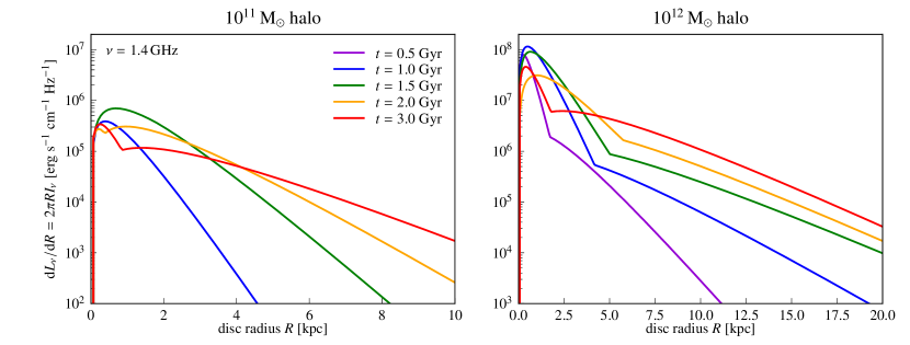
Figure 18: Differential contribution to the total radio synchrotron luminosity per radius for the small galaxy ($M_{200}=10^{11}~{}\mathrm{M}_{\odot}$, $c_{200}=12$, left column) and our Milky Way-mass galaxy ($M_{200}=10^{12}~{}\mathrm{M}_{\odot}$, $c_{200}=7$, right column) at different times (as indicated in the legend). We use the fitting functions of Eq. (42).

We observe that the local FRC decreases steeply towards large radii (see the bottom panels of Fig. 17). However, these radii show small values of the surface brightness below $\upmu\mathrm{Jy~{}arcmin}^{-2}$ (see the bottom panels of Fig. 16) which are very challenging to observe. Most importantly, these regions contribute negligibly to the total radio synchrotron luminosity as can be inferred from their differential contribution to the total radio synchrotron luminosity, $\mathrm{d}L_{\nu}/\mathrm{d}R=2\uppi RI_{\nu}~{}$ for our two haloes of $10^{11}$ and $10^{12}~{}\mathrm{M}_{\odot}$ at different times in Fig. 18. One can analytically show that $\mathrm{d}L_{\nu}/\mathrm{d}R$ for a single exponential profile, $I_{0}\exp(-R/r_{0})$, is maximsed at the scale radius. This changes for our joint exponential profiles of Eq. (42): while the synchrotron luminosity in the $10^{11}~{}\mathrm{M}_{\odot}$ halo is dominated by the external exponential, the inner exponential dominates in our Milky Way-mass galaxy at early times $t\lesssim 2$ Gyr because of the very steep central profile of the magnetic field strength. At later times, the emission in outer parts of the disc increases while it always has a subdominant contribution to the total synchrotron luminosity.

4.6 Hydrostatic pressure contribution by magnetic fields

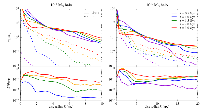
Figure 19: The top panels show radial disc profiles of the volume-averaged magnetic field strength in a disc of total height 1 kpc (dash-dotted) and equivalent hydrostatic magnetic field (solid) that is required to balance the vertical disc gravity, $B_{\mathrm{HSE}}=(8\uppi^{2}G\Sigma_{\mathrm{g}}\Sigma_{\mathrm{tot}})^{1/2}$ for the small galaxy ($M_{200}=10^{11}~{}\mathrm{M}_{\odot}$, $c_{200}=12$, left column) and our Milky Way-mass galaxy ($M_{200}=10^{12}~{}\mathrm{M}_{\odot}$, $c_{200}=7$, right column) at different times (as indicated in the legend). The bottom panels show the ratio $B/B_{\mathrm{HSE}}$, which indicates that the magnetic field plays an important role in the overall pressure balance of the ISM in the central region but not at large disc radii.

This immediately poses the question whether the integrated magnetic pressure provides a sizeable contribution to the ISM energy budget or whether it is even able to aid in driving the outflows seen in our galaxies. Assuming axisymmetry, the gravitational field of the disc is given by $\Phi_{\rm grav}(R)\approx 2\uppi G\Sigma_{\rm tot}(R)$, where $\Sigma_{\mathrm{tot}}$ is the total surface density of stars and gas. This enables us to define a hydrostatic equivalent magnetic field that balances the vertical gravitational force per unit area on the interstellar gas via

$$\frac{B_{\mathrm{HSE}}^{2}(R)}{8\uppi} =\uppi G\Sigma_{\mathrm{g}}(R)\Sigma_{\mathrm{tot}}(R),$$ (43)

$$B_{\mathrm{HSE}} \approx 15\left(\frac{\Sigma_{\mathrm{g}}}{10\,\mathrm{M}_{\odot}~{}\mathrm{pc}^{-2}}\right)^{1/2}\left(\frac{\Sigma_{\mathrm{tot}}}{100~{}\mathrm{M}_{\odot}\mathrm{pc}^{-2}}\right)^{1/2}\,\upmu\mathrm{G}.$$ (44)

Note that on circular orbits in the disc plane, the gravitational force due to the dark matter halo is exactly balanced by the centrifugal force. Hence, a field of strength $B_{\mathrm{HSE}}$ would hydrostatically counteract the gravity of the disc while any smaller field strength would either signal a system that is out of equilibrium or require a thermal and/or turbulent pressure to counteract gravity.

In Fig. 19, we compare the profile of the magnetic field strength to the equivalent hydrostatic magnetic field, $B_{\mathrm{HSE}}$, that is required to balance the vertical disc gravity for different times in our two fiducial haloes. The $B_{\mathrm{HSE}}$ profile shows that already at $t=0.5$ Gyr, the disc mass has largely assembled up to disc radii of about 5 kpc (10 kpc) for our $10^{11}$ ($10^{12}~{}\mathrm{M}_{\odot}$) haloes so that the disc gravity barely changes at these intermediate radii, but stars continue to form out of the available gas. At later times, the disc gravity moderately grows at larger radii due to gas accretion and decreases in the centre due to CR-driven galactic winds that move gas from the disc into the circumgalactic medium. The bottom panels of Fig. 19 show the contribution of the magnetic field to counteract disc gravity via the magnetic pressure force. Only at late times for radii 1–2 kpc does the magnetic field come close to $B_{\mathrm{HSE}}$ but otherwise stays subdominant, i.e., $B\lesssim B_{\mathrm{HE}}$. This implies that while magnetic pressure can contribute significantly to the total pressure balance of the ISM, it does not play an active role in driving disc winds. This can also be seen by the comparison of pure MHD simulations of isolated galaxies that are contrasted to simulations with purely advective CRs in figure 5 of Pfrommer et al. (2017a), which demonstrates that magnetic and CR pressures (in the advective transport approximation) are not powerful enough in order to drive galactic winds and hence, we require e.g., CR transport relative to the gas for launching galactic winds. We caution that additional, supernova-driven ISM turbulence could grow the magnetic field further and increase is contribution to the overall energy balance.

5 Discussion and conclusions

In this work, we studied (i) the growth of the galactic seed magnetic field through adiabatic compression and emergent small-scale dynamos driven by turbulence resulting from gravitational collapse of the proto-galaxy and velocity shear between the centrifugally supported galactic disc and hot circumgalactic medium. Using this insight, we deconstructed (ii) the radio synchrotron emission in three-dimensional MHD simulations of forming galaxies that follow the CR energy density in the one-moment approximation with the goal to understand the origin and physical processes underlying the FRC. Solving the steady-state equation for CR protons, primary, and secondary electrons enables us to reliably model the emergence of the radio emission from their formation to the starburst appearance to the quiescently star-forming stage across a range of galaxy masses from dwarfs to Milky Way sizes.

5.1 Small-scale magnetic dynamo in galaxy formation

To understand the emergence of galactic magnetic fields, we perform thorough statistical studies of the time evolution of magnetic energy, $B$–$\rho$ correlations, power spectra, and statistics of magnetic curvature $\kappa$ and curvature force density $f_{\mathrm{c}}$, for various spatial regions (centre, disc and entire halo), halo masses and at different characteristic times.

In particular, we carefully study the numerical Reynolds number of our simulations, reaching values of $\mathrm{Re}\sim 3\times 10^{2}$. We demonstrate that the growth rate of the small-scale dynamo does not only agree with our theoretical estimate and scales with the numerical grid size exactly as expected but also saturates at the turbulent energy density. Thus, this provides quantitative evidence that our employed numerical method of moving mesh magneto-hydrodynamics with Powell cleaning delivers accurate results.

We find that the magnetic energy density is exponentially amplified over ten or fourteen orders of magnitude in the Milky Way-mass galaxy, depending on the choice of our initial seed magnetic field. Initially, the magnetic field grows via adiabatic compression, nearly independent of numerical resolution. In a second phase, the small-scale dynamo emerges and grows the magnetic field fastest at the highest resolution in the galaxy centre. The small-scale dynamo starts earlier and the exponential growth rate is larger for increasing resolution and halo masses. Initially, turbulence is injected at the corrugated accretion shock, which propagates outwards. As the associated turbulence is decaying, the large velocity shear between the supersonically rotating cool disc with respect to the (partially) pressure-supported hot circumgalactic medium excites Kelvin-Helmholtz surface and body modes, which non-linearly interact and inject additional turbulence which continuously drives additional small-scale dynamos.

While our model represents a simplified model for the formation of a disc galaxy, we note that it exhibits all the essential ingredients, including a rotationally supported star-forming disc that is embedded in a warm circumgalactic medium, which has been thermalised by an accretion shock. In a more realistic galaxy, the disc-halo interface may be more structured and exhibit a smoother gradient. However, this only changes the spectrum and exact growth rates of the Kelvin-Helmholtz unstable modes (and the associated small-scale dynamo) and not the qualitative picture put forward here, as can be seen by introducing a smooth transition layer between a cold, dense stream moving at supersonic speed through the ambient hot, dilute circumgalactic medium (Berlok & Pfrommer, 2019a, b).

Using curvature statistics, we can clearly demonstrate the superposition of various small-scale dynamo modes at different densities and scales. Once the dynamo mode at the highest density comes into (approximate) equipartition with the turbulent kinetic energy at that scale, magnetic power continues to grow on large scales until saturation at the corresponding larger kinetic turbulent energy, which increases the magnetic coherence scale with time to eventually saturate its growth. Magnetic saturation is independent of our adopted initial magnetic field, which ranges from a homogeneous seed field to a magnetic dipole field that follows a strength proportional to $\rho_{\mathrm{NFW}}^{2/3}$. The latter may result from the isotropic collapse of a proto-galaxy due to magnetic flux freezing. We demonstrate that there exists a mapping between initial field strength $B_{\mathrm{init}}$ and the IGM strength $B_{\mathrm{IGM}}$ of our pre-collapsed model for the initial magnetic field so that the energy growth rates as well as the $B$–$\rho$ correlations are nearly identical (although that mapping differs for both set of comparisons).

In our model, gravitational collapse drives a starburst that quickly brings the CR and thermal energy density into approximate equipartition. We find that the magnetic field saturates at a slower rate in smaller galaxies and does not reach equipartition with the thermal and CR energy densities. Instead, its energy density saturates with the gravo-turbulent energy density that we approximate with the (subdominant) poloidal energy density and scales according to $E_{B}\propto M_{200}^{5/3}$. Interestingly, the rotational kinetic energy density in these centrifugally-dominated discs is about 100 times larger than the ‘turbulent’ kinetic energy density. The emerging magnetic pressure balances the vertical disc gravity in the centre but not at large radii. However, we anticipate that cosmological simulations of dwarf galaxies with an improved ISM model (e.g., Gutcke et al., 2021) in combination with a two-moment CR hydrodynamic scheme (e.g., Thomas & Pfrommer, 2019) can further amplify the magnetic field strength in these systems via supernova- and cosmic accretion-driven turbulence as well as modulate the impact of CR transport on the magnetic dynamo amplification with a more consistent CR diffusion coefficient in the self-confinement picture.

We show analytically, that the largest scales in the magnetic power spectrum are dominated by the exponential profile of the magnetic field in the galaxy centre and cascades down in scale consistent with the prediction from MHD turbulence. After excluding the central region where the magnetic field plays an important role in the overall pressure balance, we show that the magnetic growth in the kinematic phase follows a Kazantsev (1968) spectrum. In agreement with simulations of the fluctuating small-scale dynamo (Brandenburg & Subramanian, 2005), the Kazantsev spectrum turns over at the scale where the magnetic and turbulent energy have achieved equipartition so that the back-reaction exerted by the magnetic tension force suppresses the stretching process of eddies that are smaller than the equipartition scale. MHD turbulence imposes a spectrum on smaller scales, which follows a Kolmogorov (1941) slope.

5.2 The correlation of radio synchrotron and FIR emission

We find that the total radio synchrotron emission of the Milky Way-mass galaxy is dominated by the disc and a bright bulge that results in a CR-driven, magnetically-loaded outflow which is visible in form of faint radio bubbles. On the contrary, the edge-on view of the smaller galaxy with halo mass $10^{11}~{}\mathrm{M}_{\odot}$ shows a characteristic X-shaped radio morphology in the outflow region, which results from combining the cylindrical magnetic outflow geometry with the CR electron distribution that shows bi-conical, low-density cavities.

We show that quiescently star-forming and star-bursting galaxies with a saturated small-scale dynamo are on the FRC while galaxies with quenched dynamos—that in our simulations are realised by a strong CR-driven outflow in combination with a single starburst event caused by a one-time accretion phase and turbulent driving—fail to reach the magnetic energy that is necessary to reach the FRC. The intrinsic scatter in the FRC arises due to the following effects.

1. The radio luminosity varies due to somewhat different magnetic saturation levels that result from different seed magnetic fields at the formation time or a different formation history and magnetic dynamo efficiencies. In addition, intermittent galactic wind velocities modulate the magnetic and CR energy in the inner galactic regions that are affected by the wind and temporarily change the resulting synchrotron luminosity.

2. Different galaxy (and stellar) masses at a given SFR: the gas accretion rate decreases after the starburst phases and so does the SFR. In consequence, there are two effects that decrease the radio synchrotron luminosity at a smaller rate in comparison to the SFR. First, smaller SFRs imply smaller gas densities and smaller collisional loss rates so that the calorimetric energy fraction emitted via radio synchrotron increases. Second, the amount of injected CR energy decreases as the SFR drops but the magnetic field strengths are maintained by a dynamo action at a constant level. As a result, a galaxy is not exactly evolving along the relation towards smaller FIR flux but instead progresses towards the upper envelope of the scatter. Thus, at a given SFR, our model predicts less massive systems with high specific SFRs to populate the lower envelope of the FRC in comparison to more massive systems that are in a late evolutionary phase and show small specific SFRs.

3. A varying radio intensity with galactic inclination in combination with an anisotropic magnetic field distribution: while the face-on radio luminosity reaches about twice the value of the edge-on luminosity for toroidal field configurations (in quiescent star-forming discs), the edge-on luminosity becomes significant for substantial poloidal configurations (in strong outflows).

Our simulations show that different CR transport models modulate the magnetic dynamo efficiency and the CR electron density via CR-driven winds. Thus, an increasing (constant) CR diffusion coefficient moves galaxies to the lower envelope of the simulated FRC. It remains to be seen whether this effect contributes to the scatter in the observed FRC and whether there is a range of effective CR transport speeds at a fixed SFR.

Identifying the underlying physical processes responsible for the scatter in the FRC opens up the possibility of constructing a non-thermal fundamental plane of star-forming galaxies. Adding a third parameter (or a combination of parameters) in addition to the FIR and radio luminosities might enable to construct a lower-dimensional manifold relative to which the scatter can be reduced, thus enabling more precise SFR estimates with radio data. Our simulations suggest that observables that are sensitive to the specific SFR as well as the galactic inclination are prime candidates for such a third parameter (combination).

In agreement with observations, regions of several 100 pc within star-forming galaxies broadly obey the FRC out to disc radii, which contribute significantly to the radio emission. We find that galaxy centres show an excess of the local FRC ratio that mimics the observed complex behaviour with local extrema corresponding to highly star-forming galactic structures. These observations show a sub-linear FRC in the low-density interarm and outer region and super-linear behaviour in galaxy centres. Interestingly, the central parts of starbursts exceed the FRC by a substantial amount.

Future work that follows the CR proton and electron spectra in space and time is needed to consolidate these findings that are based on a steady-state assumption. In order to more realistically model the magnetic dynamo, future work also needs to explicitly model the supernova-driven ISM turbulence that yields a multi-phase medium. Nevertheless, we believe that we identified the critical physical processes that cause the emergence of radio emission in galaxies and the origin of the FRC. This will pave the road for using observations of non-thermal radio emission to learn about the impact of CR feedback in galaxy formation.

Data Availability

The data underlying this article will be shared on reasonable request to the corresponding author.

Appendix A Supporting material for discussions of the small-scale dynamo

In this appendix, we provide additional supporting material for the discussion of the small-scale dynamo in Sections 3.2 and 3.3 by (i) deriving the exponential growth rate of the small-scale dynamo in ideal MHD, (ii) scrutinising the time evolution of the numerical resolution in our high-resolution simulations, which is required to estimate the effective Reynolds numbers in our simulations, and (iii) by analysing the radial profile of the magnetic field strength $B$ during the initial stages of exponential growth.

A.1 Magnetic growth rate in Kolmogorov turbulence

Assuming incompressible turbulence that is driven at the outer scale $\mathscr{L}$ with a velocity $\mathscr{V}$, we define the Kolmogorov length $\ell$ (where kinetic energy is dissipated with a kinetic viscosity $\nu_{\mathrm{vis}}$):

$$\ell\equiv\left(\frac{\nu_{\mathrm{vis}}^{3}}{\dot{\epsilon}}\right)^{1/4},\quad{\rm where}\quad\dot{\epsilon}=\frac{\varv_{\lambda}^{3}}{\lambda}=\frac{\mathscr{V}^{3}}{\mathscr{L}}$$ (45)

is the energy flow rate per unit mass that is valid on all scales $\lambda$ and constant (because energy does not accumulate at any intermediate scale). Hence, we can also identify $\dot{\epsilon}=\mathscr{V}^{3}/\mathscr{L}$ with the energy injection rate into the turbulent cascade at scale $\mathscr{L}$. We obtain the corresponding velocity and time-scales at the Kolmogorov length $\ell$,

$$\varv_{\ell} =\left(\dot{\epsilon}\ell\right)^{1/3}=\left(\dot{\epsilon}\nu_{\mathrm{vis}}\right)^{1/4}=\mathscr{V}\,\mathrm{Re}^{-1/4},$$ (46)

$$\tau_{\ell} =\frac{\ell}{\varv_{\ell}}=\left(\frac{\nu_{\mathrm{vis}}}{\dot{\epsilon}}\right)^{1/2}=\tau\,\mathrm{Re}^{-1/2},$$ (47)

where we have used the definition of the Reynolds number $\mathrm{Re}$ (Eq. 14) and defined the eddy turnover time at the outer scale, $\tau=\mathscr{L}/\mathscr{V}$. Hence, we obtain the scaling of the outer to inner eddy turnover timescale or – equivalently – the inverse growth rates,

$$\frac{\Gamma_{\ell}}{\mathscr{V}/\mathscr{L}}=\frac{\tau}{\tau_{\ell}}=\mathrm{Re}^{1/2}.$$ (48)

In a small-scale dynamo, the magnetic field grows fastest at the resistive scale (Schekochihin et al., 2004; Brandenburg & Subramanian, 2005), which corresponds to the Kolmogorov scale for a magnetic Prandtl number of unity. We identify this scale with the local grid scale in ideal MHD (where the explicit kinematic viscosity and resistivity are neglected, i.e. $\nu_{\mathrm{vis}}=\eta_{\mathrm{res}}=0$ and are replaced by the numerical counterparts that operate on the grid scale). Because our moving Voronoi mesh dynamically adjust the resolution in a quasi-Lagrangian fashion (see Fig. 20), we expect the small-scale dynamo to grow fastest in the highest density regions in the galactic centre.

A.2 Numerical resolution of the moving mesh

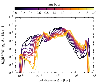
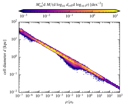
Figure 20: Quantifying the numerical resolution in our simulation of a $10^{12}~{}\mathrm{M}_{\odot}$ halo with concentration parameter $c_{200}=7$ and initially $10^{7}$ cells within the virial radius. On the left-hand side, we show the mass-weighted probability density of cell diameters, $d_{\mathrm{cell}}=(6V/\uppi)^{1/3}$ (assuming a spherical cell volume) for different times, initially spaced by 100 Myrs, and after 1 Gr, spaced by 200 Myr. On the right-hand side, we show the mass-weighted probability density of resolution elements in the $d_{\mathrm{cell}}$–$\rho$ plane (at $t=1$ Gyr), demonstrating the (almost) Lagrangian nature of the code that is manifested in the relation $d_{\mathrm{cell}}\propto\rho^{-1/3}$ (the exact expression for $d_{\mathrm{cell}}$ used in the simulation is shown with the red dash-dotted line). The density is scaled to the star formation threshold $\rho_{0}=4.05\times 10^{-25}\,\mathrm{g~{}cm}^{-3}$. The improved resolution at scaled densities $\gtrsim\rho/\rho_{0}=10^{-3}$ is due to the refinement criterion that ensures that the volume of adjacent Voronoi cells differs at most by a factor of ten.

Recent adaptive mesh-refinement simulations of magnetic field growth in clusters and galaxies have opted for a quasi-uniform maximum refinement level in the high-density regions of interest (Rieder & Teyssier, 2016; Vazza et al., 2018; Martin-Alvarez et al., 2022), which facilitates the numerical dissipation properties and enables to quote a reliable numerical Reynolds number of the flow. Because the numerical truncation error is proportional to the sum of the absolute values of sound speed and gas velocity, the schemes require an enormous resolution to resolve a small-scale dynamo (Martin-Alvarez et al., 2022), which is otherwise quenched by numerical dissipation. There are two alternatives to nevertheless resolve a small-scale dynamo: (i) increasing the integral scales $\mathscr{L}$ and $\mathscr{V}$ through feedback (Rieder & Teyssier, 2016, 2017a), or (ii) increasing the effective resolution by introducing a turbulent subgrid scheme, which enables resolving the growth of a small-scale dynamo below the formal grid resolution that would otherwise be numerically dissipated (Liu et al., 2022).

On a quasi-Lagrangian moving mesh employed here, there is no explicit control of the effective Reynolds number. Instead, the cell diameter $d_{\mathrm{cell}}=(6V/\uppi)^{1/3}=[6M/(\uppi\rho)]^{1/3}$ depends on the gas density $\rho$ and target gas mass $M$ that the code keeps constant (up to a small tolerance interval). As a result, at a given spatial resolution there is a smaller truncation error in comparison to spatially-fixed adaptive mesh refinement codes because the dominating advection error relative to the grid is significantly reduced. Increasing the velocity of the mesh-generating points would cause non-Lagrangian motion of the mesh and hence result in an increased truncation error.

Figure 20 shows the numerical resolution in our high-resolution Milky Way-like simulation. The mass-weighted probability density shows a wide spectrum of cell sizes down to a minimum diameter of 10 pc. The two-dimensional probability density of cell size and gas density demonstrates the (almost) Lagrangian nature of the code that is manifested in the relation $d_{\mathrm{cell}}\propto\rho^{-1/3}$. Using our insight that the dynamo grows fastest in the centre at the highest densities (Figs. 9 and 10), we conclude that the small-scale dynamo in the centre grows with an effective numerical resolution of 10 pc, which should be the cell size entering our estimate of the effective numerical Reynolds number in Section 3.2.

A.3 Profile of the magnetic field strength at early times

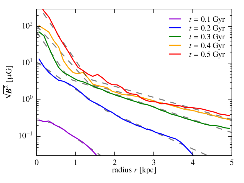
Figure 21: Radial profiles of magnetic field strength during the initial stages of exponential growth for different time (colour-coded). The profiles are well fit by a joint exponential profile (dashed lines) of Eq. (49).

Table 3: Fitting parameters for the radial magnetic profiles $B(r)$ of the simulation of the $10^{12}~{}\mathrm{M}_{\odot}$ halo with concentration $c_{200}=7$, and the ‘CR diff’ model of Fig. 21. The joint exponential profile in Eq. (49) is characterised by a normalisation $B_{0}$, a transition radius $r_{\mathrm{tr}}$, and the scale radii of the inner and outer exponentials, $r_{0}$ and $r_{1}$.

simulation time	$B_{0}$	$r_{\mathrm{tr}}$	$r_{0}$	$r_{1}$
|[Gyr]	[$\upmu$G]	[kpc]	[kpc]	[kpc]
0.1	0.3	0.5	2.1	0.6
0.2	10.8	1.8	0.6	0.9
0.3	71.6	0.8	0.3	1.2
0.4	105.4	1.4	0.4	1.6
0.5	430.2	1.3	0.3	1.4

Figure 21 shows the radial profiles of $B$ at different times separated by 0.1 Gyr. We see the development of a steep inner and a more shallower outer profile after $t\approx 0.2$ Gyr. Hence, we fit the three-dimensional radial profile of the magnetic field with two joint exponentials that describe $B$ in two regions separated by a transition radius $r_{\mathrm{tr}}$, i.e., a four-parameter fit defined by

$$B(r)=\left\{\begin{array}[]{ll}B_{0}\mathrm{e}^{-r/r_{0}},&\mathrm{if}~{}~{}r<r_{\mathrm{tr}},\\ B_{0}\mathrm{e}^{-r_{\mathrm{tr}}/r_{0}-(r-r_{\mathrm{tr}})/r_{1}},&\mathrm{if}~{}~{}r\geq{r_{\mathrm{tr}}}.\end{array}\right.$$ (49)

All fitting parameters are given in Table 3. Note that at $t\gtrsim 0.2$ Gyr the inner scale radius is rather constant, $r_{0}\sim 0.3$ to 0.4 kpc.

Note that angular momentum conservation causes the disc to flatten and hence challenges the simplified picture of a spherically symmetric magnetic field profile (see Fig. 5). While the central region exhibits quasi-spherical density and magnetic profiles (especially at early times), after the formation of a galactic disc, turbulence on scales larger than the disc scale height becomes anisotropic. We postpone a more detailed analysis of the effects of anisotropy on the small-scale dynamo in the disc and disc-halo interface to future work and note that instead of using a power spectrum analysis, this would likely require adopting azimuthally dependent velocity structure functions.

Appendix B Comparing different magnetic initial conditions

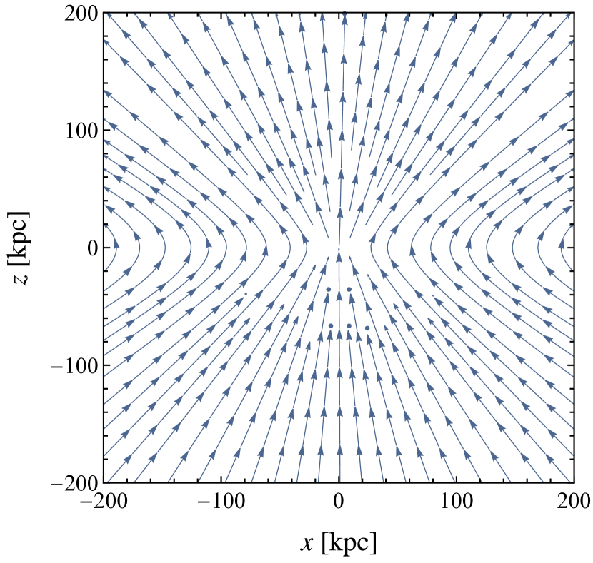
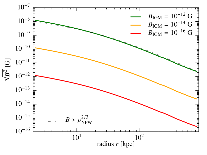
Figure 22: Initial magnetic field distribution in our flux-freezing model with a dipole-like topology (left-hand panel). We superpose the individual magnetic dipoles so that the azimuthally averaged field strength is proportional to $\rho_{\mathrm{NFW}}^{2/3}$ (right-hand panel). We simulate three models of our $10^{12}\,\mathrm{M}_{\odot}$ halo (with virial radius $r_{200}\approx 206$ kpc) that differ in their assumed magnetic field strength of the IGM, $B_{\mathrm{IGM}}$.

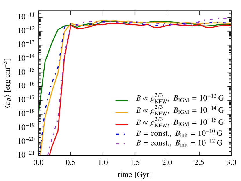
Figure 23: Time evolution of volume-averaged magnetic energy densities in a disc of radius 10 kpc and total height 1 kpc of a $10^{12}~{}\mathrm{M}_{\odot}$ halo with concentration $c_{200}=7$ and initially $10^{6}$ cells within the virial radius. We compare simulations with different initial magnetic field configurations: our flux-freezing models with a dipole-like magnetic topology, which scale with the gas density (solid lines), are confronted to simulations with an initially constant magnetic field (dash-dotted). This shows that the small-scale dynamo can more easily amplify the pre-compressed magnetic field so that the exponential dynamo growth rate of a constant initial magnetic field is equivalent to a pre-compressed field with a $10^{4}$ times smaller IGM field strength.

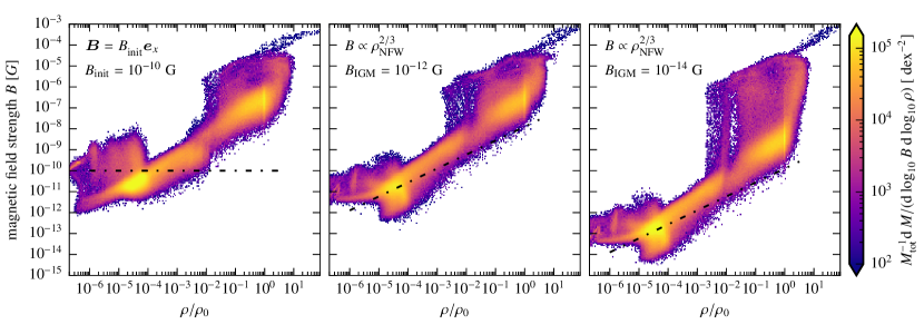
Figure 24: Mass-weighted probability density of magnetic field strength $B$ and mass density, $\rho$, in the galactic halo for three different initial magnetic field models at $t=2$ Gyr. All gas densities are scaled to the star formation threshold $\rho_{0}=4.05\times 10^{-25}\,\mathrm{g~{}cm}^{-3}$. From left to right, we show the constant field model with $B_{\mathrm{init}}=10^{-10}$ G, and two flux-freezing models with $B_{\mathrm{IGM}}=10^{-12}$ and $10^{-14}$ G. The initial distributions are shown with dash-dotted lines and we use simulations of a $10^{12}~{}\mathrm{M}_{\odot}$ halo that initially have $10^{6}$ cells within the virial radius. Note that the distributions in the first two panels are very similar.

In order to study the dependence of our conclusions on the choice of the initial magnetic field distribution, we consider two types of configurations. First, we adopt a constant initial magnetic field $\textbf{{B}}=B_{\mathrm{init}}\textbf{{e}}_{x}$, where $B_{\mathrm{init}}=10^{-10}$ and $10^{-12}$ G. Second, if the initial halo field results from isotropic collapse, magnetic flux freezing implies a scaling $B\propto\rho^{2/3}$. We preserve the constraint $\bm{\nabla}\bm{\cdot}\textbf{{B}}=0$ by deriving the magnetic field from its vector potential A. Inspired by Dubois & Teyssier (2010), our initial magnetic field distribution is a superposition of small magnetic dipoles that are aligned with the $z$ axis and have a strength proportional to $\rho^{2/3}$ so that they add up to a global large scale dipole-like topology on the halo scale albeit with a different radial behaviour.

For our flux-freezing initial conditions, we assume that gas and dark matter trace the NFW profile (Navarro et al., 1997), which we slightly soften at the centre (below 0.1 kpc) to introduce a core into the gas, allowing for a “quiet” start of the simulations. Outside, the gas mass density is given by

$$\rho(r)=\rho_{\mathrm{NFW}}(r)\frac{\Omega_{\mathrm{b}}}{\Omega_{\mathrm{m}}},$$ (50)

where $\Omega_{\mathrm{b}}$ and $\Omega_{\mathrm{m}}$ are the baryon and total mass density in units of the critical density for geometrical closure of the universe, $\rho_{\mathrm{cr}}$, and the NFW profile is given by

$$\rho_{\mathrm{NFW}}(r) =\frac{\delta_{\mathrm{c}}\rho_{\mathrm{cr}}}{r/r_{\mathrm{s}}(1+r/r_{\mathrm{s}})^{2}},$$ (51)

$$\delta_{\mathrm{c}} =\frac{200}{3}\,c_{200}^{3}\left[\ln\left(1+c_{200}\right)-\frac{c_{200}}{1+c_{200}}\right]^{-1},$$ (52)

$$r_{\mathrm{s}} =\frac{r_{200}}{c_{\mathrm{200}}}=\left(\frac{GM_{200}}{c_{\mathrm{200}}^{3}\,100H^{2}(a)}\right)^{1/3},$$ (53)

where $r=\sqrt{x^{2}+y^{2}+z^{2}}$, and the Hubble function at the cosmic scale factor $a$ is $H(a)=H_{0}\sqrt{\Omega_{\Lambda}+\Omega_{\mathrm{m}}a^{-3}}$, where $H_{0}$ is the current day value and $\Omega_{\Lambda}$ is the density parameter of the cosmological constant. Using the mean density of the IGM, $\rho_{\mathrm{IGM}}=\rho_{\mathrm{cr}}\Omega_{\mathrm{b}}$, we can write down the vector potential,

$$\textbf{{A}}=B_{\mathrm{IGM}}\,\left[\frac{\rho(r)}{\rho_{\mathrm{IGM}}}\right]^{2/3}\left(\begin{array}[]{l}-y\\ \,~{}~{}x\\ \,~{}~{}0\end{array}\right).$$ (57)

The solenoidal (divergence-free) magnetic field reads

B $$=\bm{\nabla}\bm{\times}\textbf{{A}}$$ (58)

$$=\frac{2B_{\mathrm{IGM}}}{3r^{8/3}(r+r_{\mathrm{s}})}\left[\frac{r_{\mathrm{s}}^{3}\,\delta_{\mathrm{c}}\,\Omega_{\mathrm{m}}^{-1}}{(r+r_{\mathrm{s}})^{2}}\right]^{2/3}\left(\begin{array}[]{l}xz(3r+r_{\mathrm{s}})\\ yz(3r+r_{\mathrm{s}})\\ 3rz^{2}+(2r^{2}+z^{2})r_{\mathrm{s}}\end{array}\right),$$ (62)

which depends on the parameters $B_{\mathrm{IGM}}$, $M_{200}$, and $c_{200}$ (see Table LABEL:tab:simulations-overview for our choices), and we adopt the currently favoured concordance cosmological model at the present time with $\Omega_{\mathrm{m}}=0.315$, $\Omega_{\Lambda}=0.685$, and $H_{0}=70~{}\mathrm{km~{}s}^{-1}~{}\mathrm{Mpc}^{-1}$.

Figure 22 demonstrates that the initial magnetic field topology resembles a dipole-like structure that is aligned with the $z$ axis (left-hand panel) and that the azimuthally averaged field strength decreases with radius as $\rho_{\mathrm{NFW}}^{2/3}$ (right-hand panel). Defining the virial radius $r_{200}$ such that the average density contained in the spherical volume $4/3{\pi}r_{200}^{3}$ is 200 times the critical density of the universe, we get $r_{200}\approx 206$ kpc for our $10^{12}\,\mathrm{M}_{\odot}$ halo with a concentration parameter $c_{200}=7$. Hence, the average magnetic profile approaches $B_{\mathrm{IGM}}$ only beyond $5r_{200}$ and assumes average values of approximately $30\,B_{\mathrm{IGM}}$ at the virial radius and $10^{4}\,B_{\mathrm{IGM}}$ at $0.01r_{200}$.

In Fig. 23, we compare the time evolution of volume-averaged magnetic energy densities in the gaseous galactic discs for different initial magnetic configurations. While the models differ in their exponential growth rate, they all saturate at the same level in equipartition with the turbulent energy density, as discussed in Section 3.1. The growth rate of the small-scale dynamo increases with a larger initial magnetic field strengths and the dynamo can more easily amplify the pre-compressed magnetic field of our flux-freezing model. A comparison of the different field configurations shows that the exponential dynamo growth rate of a constant initial magnetic field is equivalent to a pre-compressed field with a $10^{4}$ times smaller IGM field strength. Thus, this empirical comparison suggests that the magnetic field strength at around $0.01r_{200}$ is responsible for setting the dynamo growth rate in our moving-mesh finite-volume hydrodynamics. More work is needed to explore the full dependencies of this finding on the numerical method and exact magnetic configuration.

Figure 24 shows the distribution of the gas mass in the magnetic field strength-mass density plane for three different initial magnetic field models at $t=2$ Gyr, i.e., an epoch well into the saturated regime of the dynamo. There are two branches visible: a lower branch that reflects the halo field with approximately $B\propto\rho$ and an upper branch characterising the disc field, which dominates the total magnetic energy. Those branches are connected by a vertical bridge across which the dynamo exponentially amplifies the magnetic field, which is even more clearly visible in the panel to the right-hand side. As expected, the upper branch with the disc field is similar in all three models, which is a consequence of the equipartition magnetic field in the saturated dynamo state.

Interestingly, the distributions of the constant initial magnetic field with $B_{\mathrm{init}}=10^{-10}$ G and the flux-freezing model with $B_{\mathrm{IGM}}=10^{-12}$ G very closely resemble each other, while the model on the right-hand side shows a halo magnetic field that is lower by a factor of 100. We have seen that the dynamo growth rates of the models on the left- and right-hand panels of Fig. 24 are equal. This demonstrates while there is no exact one-to-one mapping of constant initial field and flux-freezing models, we can find close resemblances of specific properties in both models. Most importantly, the mapping between the magnetic growth rates of the two models (Fig. 23) and our power spectrum analysis in Section 3.3 show that most of the growth of the magnetic field is caused by a small-scale dynamo and not by adiabatic compression as a result of magnetic flux-freezing.

Appendix C Spectral resolution study

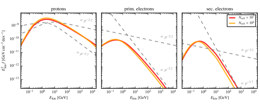
Figure 25: Resolution study of steady-state CR spectra in the galactic disc of our simulation of a $10^{12}~{}\mathrm{M}_{\odot}$ halo with concentration parameter $c_{200}=7$ at $t=1$ Gyr. The CR spectra $E_{\mathrm{kin}}^{2}f=(\ln 10)^{-1}E_{\mathrm{kin}}\mathrm{d}N/(\mathrm{d}\log_{10}E_{\mathrm{kin}}\,\mathrm{d}V)$ are volume averaged over a cylinder of a radius that includes 99 per cent of the total radio luminosity and a height above and below the mid-plane that is equal to the scale-height of the gas density. We compare simulations with initially $10^{6}$ and $10^{7}$ Voronoi cells within the virial radius and show from left to right the scaled kinetic energy spectra of CR protons, primary electrons and secondary electrons and positrons. The dashed lines represent pure power-law momentum spectra with the indicated momentum spectral indices for comparison.

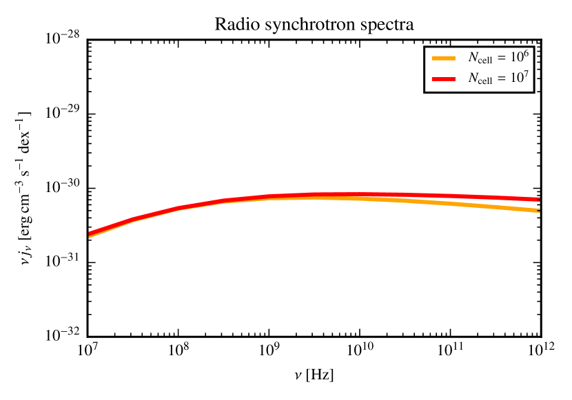
Figure 26: Resolution study of total radio synchrotron spectra of our simulation of a $10^{12}~{}\mathrm{M}_{\odot}$ halo with concentration parameter $c_{200}=7$ at $t=1$ Gyr. The total radio spectrum $\nu j_{\nu}=(\ln 10)^{-1}\mathrm{d}N_{\gamma}/(\mathrm{d}\log_{10}\nu\,\mathrm{d}V\mathrm{d}t)$ is dominated by primary CR electrons and is numerically fully converged at energies $\lesssim 100$ GHz.

The radio luminosity depends on the magnetic field strengths and CR spectra. The magnetic energy saturates early on in the galactic evolution in equilibrium with the turbulent kinetic energy and is numerically well converged. In Fig. 25, wee assess the numerical convergence of our steady-state spectra of CR protons, primary and secondary electrons. While the low-energy part ($E_{\mathrm{kin}}\lesssim 10$ GeV) of the CR spectra are well converged, our low-resolution spectra fall slightly short of the high-resolution analogues at larger energies. Because the total radio spectra in our ‘CR diff’ models are dominated by primary CR electrons (Werhahn et al., 2021c), which are well converged at kinetic energies $\lesssim 10$ GeV, we find that our radio luminosities at frequencies $\lesssim 100$ GHz are also numerically well converged (see Fig. 26).

References

- Abramowitz & Stegun (1965) Abramowitz M., Stegun I. A., 1965, Handbook of mathematical functions. New York: Dover
- Aharonian et al. (2010) Aharonian F. A., Kelner S. R., Prosekin A. Y., 2010, Pys. Rev. D, 82, 043002
- Arzoumanian et al. (2011) Arzoumanian D., et al., 2011, A&A, 529, L6
- Basu et al. (2012) Basu A., Roy S., Mitra D., 2012, ApJ, 756, 141
- Basu et al. (2017) Basu A., Roychowdhury S., Heesen V., Beck R., Brinks E., Westcott J., Hindson L., 2017, MNRAS, 471, 337
- Beck & Golla (1988) Beck R., Golla G., 1988, A&A, 191, L9
- Bell (2003) Bell E. F., 2003, ApJ, 586, 794
- Berlok & Pfrommer (2019a) Berlok T., Pfrommer C., 2019a, MNRAS, 485, 908
- Berlok & Pfrommer (2019b) Berlok T., Pfrommer C., 2019b, MNRAS, 489, 3368
- Białłas et al. (1976) Białłas A., Bleszyński M., Czyż W., 1976, Nuclear Physics B, 111, 461
- Bicay & Helou (1990) Bicay M. D., Helou G., 1990, ApJ, 362, 59
- Blasi (2010) Blasi P., 2010, MNRAS, 402, 2807
- Booth et al. (2013) Booth C. M., Agertz O., Kravtsov A. V., Gnedin N. Y., 2013, ApJ, 777, L16
- Boulares & Cox (1990) Boulares A., Cox D. P., 1990, ApJ, 365, 544
- Brandenburg & Subramanian (2005) Brandenburg A., Subramanian K., 2005, Phys. Rep., 417, 1
- Breitschwerdt et al. (2002) Breitschwerdt D., Dogiel V. A., Völk H. J., 2002, A&A, 385, 216
- Buck et al. (2020) Buck T., Pfrommer C., Pakmor R., Grand R. J. J., Springel V., 2020, MNRAS, 497, 1712
- Buckman et al. (2020) Buckman B. J., Linden T., Thompson T. A., 2020, MNRAS, 494, 2679
- Bustard et al. (2020) Bustard C., Zweibel E. G., D’Onghia E., Gallagher J. S. I., Farber R., 2020, ApJ, 893, 29
- Butsky & Quinn (2018) Butsky I. S., Quinn T. R., 2018, ApJ, 868, 108
- Butsky et al. (2017) Butsky I., Zrake J., Kim J.-h., Yang H.-I., Abel T., 2017, ApJ, 843, 113
- Butsky et al. (2020) Butsky I. S., Fielding D. B., Hayward C. C., Hummels C. B., Quinn T. R., Werk J. K., 2020, ApJ, 903, 77
- Calzetti et al. (2000) Calzetti D., Armus L., Bohlin R. C., Kinney A. L., Koornneef J., Storchi-Bergmann T., 2000, ApJ, 533, 682
- Caprioli & Spitkovsky (2014) Caprioli D., Spitkovsky A., 2014, ApJ, 783, 91
- Cerri et al. (2017) Cerri S. S., Gaggero D., Vittino A., Evoli C., Grasso D., 2017, J. Cosmology Astropart. Phys., 2017, 019
- Chabrier (2003) Chabrier G., 2003, PASP, 115, 763
- Chan et al. (2019) Chan T. K., Kereš D., Hopkins P. F., Quataert E., Su K. Y., Hayward C. C., Faucher-Giguère C. A., 2019, MNRAS, 488, 3716
- Childress & Gilbert (1995) Childress S., Gilbert A. D., 1995, Stretch, Twist, Fold
- Commerçon et al. (2019) Commerçon B., Marcowith A., Dubois Y., 2019, A&A, 622, A143
- Condon (1992) Condon J. J., 1992, ARA&A, 30, 575
- Côté et al. (2016) Côté B., Ritter C., O’Shea B. W., Herwig F., Pignatari M., Jones S., Fryer C. L., 2016, ApJ, 824, 82
- Crocco (1937) Crocco L., 1937, Z. angew. Math. Mech., 17, 1
- Dashyan & Dubois (2020) Dashyan G., Dubois Y., 2020, A&A, 638, A123
- Domingo-Santamaría & Torres (2005) Domingo-Santamaría E., Torres D. F., 2005, A&A, 444, 403
- Drummond & Muench (1991) Drummond I. T., Muench W., 1991, Journal of Fluid Mechanics, 225, 529
- Dubois & Teyssier (2010) Dubois Y., Teyssier R., 2010, A&A, 523, A72
- Dumas et al. (2011) Dumas G., Schinnerer E., Tabatabaei F. S., Beck R., Velusamy T., Murphy E., 2011, AJ, 141, 41
- Eichmann & Becker Tjus (2016) Eichmann B., Becker Tjus J., 2016, ApJ, 821, 87
- Evoli et al. (2017) Evoli C., Gaggero D., Vittino A., Di Bernardo G., Di Mauro M., Ligorini A., Ullio P., Grasso D., 2017, J. Cosmology Astropart. Phys., 2017, 015
- Evoli et al. (2019) Evoli C., Aloisio R., Blasi P., 2019, Phys. Rev. D, 99, 103023
- Evoli et al. (2020) Evoli C., Morlino G., Blasi P., Aloisio R., 2020, Phys. Rev. D, 101, 023013
- Farber et al. (2018) Farber R., Ruszkowski M., Yang H. Y. K., Zweibel E. G., 2018, ApJ, 856, 112
- Fryer (1999) Fryer C. L., 1999, ApJ, 522, 413
- Gaisser (1990) Gaisser T. K., 1990, Cosmic rays and particle physics. Cambridge University Press
- Gent et al. (2013) Gent F. A., Shukurov A., Sarson G. R., Fletcher A., Mantere M. J., 2013, MNRAS, 430, L40
- Genzel et al. (2008) Genzel R., et al., 2008, ApJ, 687, 59
- Girichidis et al. (2016a) Girichidis P., et al., 2016a, MNRAS, 456, 3432
- Girichidis et al. (2016b) Girichidis P., et al., 2016b, ApJ, 816, L19
- Girichidis et al. (2018) Girichidis P., Naab T., Hanasz M., Walch S., 2018, MNRAS, 479, 3042
- Girichidis et al. (2020) Girichidis P., Pfrommer C., Hanasz M., Naab T., 2020, MNRAS, 491, 993
- Girichidis et al. (2022) Girichidis P., Pfrommer C., Pakmor R., Springel V., 2022, MNRAS, 510, 3917
- Goldreich & Sridhar (1995) Goldreich P., Sridhar S., 1995, ApJ, 438, 763
- Gutcke et al. (2021) Gutcke T. A., Pakmor R., Naab T., Springel V., 2021, MNRAS, 501, 5597
- Hanasz & Lesch (2003) Hanasz M., Lesch H., 2003, A&A, 412, 331
- Hanasz et al. (2013) Hanasz M., Lesch H., Naab T., Gawryszczak A., Kowalik K., Wóltański D., 2013, ApJ, 777, L38
- Heesen et al. (2009) Heesen V., Krause M., Beck R., Dettmar R. J., 2009, A&A, 506, 1123
- Heesen et al. (2014) Heesen V., Brinks E., Leroy A. K., Heald G., Braun R., Bigiel F., Beck R., 2014, AJ, 147, 103
- Heesen et al. (2019) Heesen V., et al., 2019, A&A, 622, A8
- Helou et al. (1985) Helou G., Soifer B. T., Rowan-Robinson M., 1985, ApJ, 298, L7
- Hippelein et al. (2003) Hippelein H., Haas M., Tuffs R. J., Lemke D., Stickel M., Klaas U., Völk H. J., 2003, A&A, 407, 137
- Hoernes et al. (1998) Hoernes P., Berkhuijsen E. M., Xu C., 1998, A&A, 334, 57
- Hopkins et al. (2020) Hopkins P. F., et al., 2020, MNRAS, 492, 3465
- Hughes et al. (2006) Hughes A., Wong T., Ekers R., Staveley-Smith L., Filipovic M., Maddison S., Fukui Y., Mizuno N., 2006, MNRAS, 370, 363
- Jacob et al. (2018) Jacob S., Pakmor R., Simpson C. M., Springel V., Pfrommer C., 2018, MNRAS, 475, 570
- Ji et al. (2020) Ji S., et al., 2020, MNRAS, 496, 4221
- Jiang & Oh (2018) Jiang Y.-F., Oh S. P., 2018, ApJ, 854, 5
- Jubelgas et al. (2008) Jubelgas M., Springel V., Enßlin T., Pfrommer C., 2008, A&A, 481, 33
- Kazantsev (1968) Kazantsev A. P., 1968, Soviet Journal of Experimental and Theoretical Physics, 26, 1031
- Kelner et al. (2006) Kelner S. R., Aharonian F. A., Bugayov V. V., 2006, Phys. Rev. D, 74, 034018
- Kennicutt (1998a) Kennicutt Jr. R. C., 1998a, ARA&A, 36, 189
- Kennicutt (1998b) Kennicutt Jr. R. C., 1998b, ApJ, 498, 541
- Klessen & Hennebelle (2010) Klessen R. S., Hennebelle P., 2010, A&A, 520, A17
- Kolmogorov (1941) Kolmogorov A., 1941, The Proceedings of the USSR Academy of Sciences, 30, 301
- Krause et al. (2020) Krause M., et al., 2020, A&A, 639, A112
- Lacki & Thompson (2010) Lacki B. C., Thompson T. A., 2010, ApJ, 717, 196
- Lacki & Thompson (2013) Lacki B. C., Thompson T. A., 2013, ApJ, 762, 29
- Lacki et al. (2010) Lacki B. C., Thompson T. A., Quataert E., 2010, ApJ, 717, 1
- Lacki et al. (2011) Lacki B. C., Thompson T. A., Quataert E., Loeb A., Waxman E., 2011, ApJ, 734, 107
- Lisenfeld et al. (1996) Lisenfeld U., Völk H. J., Xu C., 1996, A&A, 306, 677
- Liu et al. (2022) Liu Y., Kretschmer M., Teyssier R., 2022, MNRAS, 513, 6028
- Lopez-Rodriguez et al. (2021) Lopez-Rodriguez E., Guerra J. A., Asgari-Targhi M., Schmelz J. T., 2021, ApJ, 914, 24
- Mandelker et al. (2016) Mandelker N., Padnos D., Dekel A., Birnboim Y., Burkert A., Krumholz M. R., Steinberg E., 2016, MNRAS, 463, 3921
- Mandelker et al. (2020) Mandelker N., Nagai D., Aung H., Dekel A., Birnboim Y., van den Bosch F. C., 2020, MNRAS, 494, 2641
- Martin (2014) Martin P., 2014, A&A, 564, A61
- Martin-Alvarez et al. (2022) Martin-Alvarez S., Devriendt J., Slyz A., Sijacki D., Richardson M. L. A., Katz H., 2022, MNRAS, 513, 3326
- Matthews et al. (2021) Matthews A. M., Condon J. J., Cotton W. D., Mauch T., 2021, ApJ, 914, 126
- Miskolczi et al. (2019) Miskolczi A., et al., 2019, A&A, 622, A9
- Miyoshi & Kusano (2005) Miyoshi T., Kusano K., 2005, J. Comput. Phys., 208, 315
- Molnár et al. (2021) Molnár D. C., et al., 2021, MNRAS, 504, 118
- Murphy et al. (2008) Murphy E. J., Helou G., Kenney J. D. P., Armus L., Braun R., 2008, ApJ, 678, 828
- Navarro et al. (1997) Navarro J. F., Frenk C. S., White S. D. M., 1997, ApJ, 490, 493
- Ogrodnik et al. (2021) Ogrodnik M. A., Hanasz M., Wóltański D., 2021, ApJS, 253, 18
- Padnos et al. (2018) Padnos D., Mandelker N., Birnboim Y., Dekel A., Krumholz M. R., Steinberg E., 2018, MNRAS, 477, 3293
- Paglione & Abrahams (2012) Paglione T. A. D., Abrahams R. D., 2012, ApJ, 755, 106
- Pais & Pfrommer (2020) Pais M., Pfrommer C., 2020, MNRAS, 498, 5557
- Pais et al. (2018) Pais M., Pfrommer C., Ehlert K., Pakmor R., 2018, MNRAS, 478, 5278
- Pais et al. (2020) Pais M., Pfrommer C., Ehlert K., Werhahn M., Winner G., 2020, MNRAS, 496, 2448
- Pakmor & Springel (2013) Pakmor R., Springel V., 2013, MNRAS, 432, 176
- Pakmor et al. (2011) Pakmor R., Bauer A., Springel V., 2011, MNRAS, 418, 1392
- Pakmor et al. (2016a) Pakmor R., Springel V., Bauer A., Mocz P., Munoz D. J., Ohlmann S. T., Schaal K., Zhu C., 2016a, MNRAS, 455, 1134
- Pakmor et al. (2016b) Pakmor R., Pfrommer C., Simpson C. M., Kannan R., Springel V., 2016b, MNRAS, 462, 2603
- Pakmor et al. (2016c) Pakmor R., Pfrommer C., Simpson C. M., Springel V., 2016c, ApJ, 824, L30
- Pakmor et al. (2017) Pakmor R., et al., 2017, MNRAS, 469, 3185
- Pakmor et al. (2018) Pakmor R., Guillet T., Pfrommer C., Gómez F. A., Grand R. J. J., Marinacci F., Simpson C. M., Springel V., 2018, MNRAS, 481, 4410
- Pakmor et al. (2020) Pakmor R., et al., 2020, MNRAS, 498, 3125
- Persic et al. (2008) Persic M., Rephaeli Y., Arieli Y., 2008, A&A, 486, 143
- Pfrommer et al. (2017a) Pfrommer C., Pakmor R., Schaal K., Simpson C. M., Springel V., 2017a, MNRAS, 465, 4500
- Pfrommer et al. (2017b) Pfrommer C., Pakmor R., Simpson C. M., Springel V., 2017b, ApJ, 847, L13
- Powell et al. (1999) Powell K. G., Roe P. L., Linde T. J., Gombosi T. I., De Zeeuw D. L., 1999, J. Comput. Phys., 154, 284
- Priestley & Whitworth (2021) Priestley F. D., Whitworth A. P., 2021, MNRAS,
- Rathjen et al. (2021) Rathjen T.-E., et al., 2021, MNRAS, 504, 1039
- Rieder & Teyssier (2016) Rieder M., Teyssier R., 2016, MNRAS, 457, 1722
- Rieder & Teyssier (2017a) Rieder M., Teyssier R., 2017a, MNRAS, 471, 2674
- Rieder & Teyssier (2017b) Rieder M., Teyssier R., 2017b, MNRAS, 472, 4368
- Rodrigues et al. (2016) Rodrigues L. F. S., Sarson G. R., Shukurov A., Bushby P. J., Fletcher A., 2016, ApJ, 816, 2
- Ruszkowski et al. (2017) Ruszkowski M., Yang H. Y. K., Zweibel E., 2017, ApJ, 834, 208
- Rybicki & Lightman (1979) Rybicki G. B., Lightman A. P., 1979, Radiative processes in astrophysics. New York, Wiley-Interscience
- Salem & Bryan (2014) Salem M., Bryan G. L., 2014, MNRAS, 437, 3312
- Salem et al. (2014) Salem M., Bryan G. L., Hummels C., 2014, ApJ, 797, L18
- Salem et al. (2016) Salem M., Bryan G. L., Corlies L., 2016, MNRAS, 456, 582
- Schekochihin et al. (2001) Schekochihin A., Cowley S., Maron J., Malyshkin L., 2001, Phys. Rev. E, 65, 016305
- Schekochihin et al. (2004) Schekochihin A. A., Cowley S. C., Taylor S. F., Maron J. L., McWilliams J. C., 2004, ApJ, 612, 276
- Schlickeiser (2002) Schlickeiser R., 2002, Cosmic Ray Astrophysics
- Schmidt (1959) Schmidt M., 1959, ApJ, 129, 243
- Schneider et al. (2012) Schneider N., et al., 2012, A&A, 540, L11
- Schober et al. (2013) Schober J., Schleicher D. R. G., Klessen R. S., 2013, A&A, 560, A87
- Semenov et al. (2021) Semenov V. A., Kravtsov A. V., Caprioli D., 2021, ApJ, 910, 126
- Simpson et al. (2016) Simpson C. M., Pakmor R., Marinacci F., Pfrommer C., Springel V., Glover S. C. O., Clark P. C., Smith R. J., 2016, ApJ, 827, L29
- Springel (2010) Springel V., 2010, MNRAS, 401, 791
- Springel & Hernquist (2003) Springel V., Hernquist L., 2003, MNRAS, 339, 289
- Spruit (2013) Spruit H. C., 2013, arXiv e-prints, p. arXiv:1301.5572
- Stein et al. (2020) Stein Y., et al., 2020, A&A, 639, A111
- Steinwandel et al. (2019) Steinwandel U. P., Beck M. C., Arth A., Dolag K., Moster B. P., Nielaba P., 2019, MNRAS, 483, 1008
- Stephens & Badhwar (1981) Stephens S. A., Badhwar G. D., 1981, Ap&SS, 76, 213
- Tabatabaei et al. (2007) Tabatabaei F. S., et al., 2007, A&A, 466, 509
- Thomas & Pfrommer (2019) Thomas T., Pfrommer C., 2019, MNRAS, 485, 2977
- Thomas & Pfrommer (2022) Thomas T., Pfrommer C., 2022, MNRAS, 509, 4803
- Thomas et al. (2020) Thomas T., Pfrommer C., Enßlin T., 2020, ApJ, 890, L18
- Thomas et al. (2021) Thomas T., Pfrommer C., Pakmor R., 2021, MNRAS, 503, 2242
- Thomas et al. (2022) Thomas T., Pfrommer C., Pakmor R., 2022, arXiv e-prints, p. arXiv:2203.12029
- Thompson et al. (2006) Thompson T. A., Quataert E., Waxman E., Murray N., Martin C. L., 2006, ApJ, 645, 186
- Thompson et al. (2007) Thompson T. A., Quataert E., Waxman E., 2007, ApJ, 654, 219
- Torres (2004) Torres D. F., 2004, ApJ, 617, 966
- Tüllmann et al. (2000) Tüllmann R., Dettmar R.-J., Soida M., Urbanik M., Rossa J., 2000, A&A, 364, L36
- Uhlig et al. (2012) Uhlig M., Pfrommer C., Sharma M., Nath B. B., Enßlin T. A., Springel V., 2012, MNRAS, 423, 2374
- Vazza et al. (2018) Vazza F., Brunetti G., Brüggen M., Bonafede A., 2018, MNRAS, 474, 1672
- Vink (2012) Vink J., 2012, A&ARv, 20, 49
- Völk (1989) Völk H. J., 1989, A&A, 218, 67
- Weinberger et al. (2020) Weinberger R., Springel V., Pakmor R., 2020, ApJS, 248, 32
- Werhahn et al. (2021a) Werhahn M., Pfrommer C., Girichidis P., Puchwein E., Pakmor R., 2021a, MNRAS, 505, 3273
- Werhahn et al. (2021b) Werhahn M., Pfrommer C., Girichidis P., Winner G., 2021b, MNRAS, 505, 3295
- Werhahn et al. (2021c) Werhahn M., Pfrommer C., Girichidis P., 2021c, MNRAS, 508, 4072
- Whitworth et al. (2021) Whitworth A. P., Priestley F. D., Arzoumanian D., 2021, MNRAS, 508, 2736
- Wiener et al. (2017) Wiener J., Pfrommer C., Oh S. P., 2017, MNRAS, 467, 906
- Winner et al. (2019) Winner G., Pfrommer C., Girichidis P., Pakmor R., 2019, MNRAS, 488, 2235
- Winner et al. (2020) Winner G., Pfrommer C., Girichidis P., Werhahn M., Pais M., 2020, MNRAS, 499, 2785
- Yang et al. (2018) Yang R.-z., Kafexhiu E., Aharonian F., 2018, A&A, 615, A108
- Yang et al. (2019) Yang Y., Wan M., Matthaeus W. H., Shi Y., Parashar T. N., Lu Q., Chen S., 2019, Physics of Plasmas, 26, 072306
- Yoast-Hull et al. (2013) Yoast-Hull T. M., Everett J. E., Gallagher J. S. I., Zweibel E. G., 2013, ApJ, 768, 53
- Yoast-Hull et al. (2015) Yoast-Hull T. M., Gallagher J. S., Zweibel E. G., 2015, MNRAS, 453, 222
- Yoast-Hull et al. (2016) Yoast-Hull T. M., Gallagher J. S., Zweibel E. G., 2016, MNRAS, 457, L29
- Yun et al. (2001) Yun M. S., Reddy N. A., Condon J. J., 2001, ApJ, 554, 803
- Zeldovich et al. (1983) Zeldovich I. B., Ruzmaikin A. A., Sokolov D. D., eds, 1983, Magnetic fields in astrophysics, Gordon and Breach, Vol. 3
- Zirakashvili & Aharonian (2007) Zirakashvili V. N., Aharonian F., 2007, A&A, 465, 695
- de Cea del Pozo et al. (2009) de Cea del Pozo E., Torres D. F., Rodriguez Marrero A. Y., 2009, ApJ, 698, 1054
- de Jong et al. (1985) de Jong T., Klein U., Wielebinski R., Wunderlich E., 1985, A&A, 147, L6
- van der Kruit (1971) van der Kruit P. C., 1971, A&A, 15, 110
- van der Kruit (1973) van der Kruit P. C., 1973, A&A, 29, 263