AutoReCon: Neural Architecture Search-based Reconstruction for Data-free Compression

Abstract

Data-free compression raises a new challenge because the original training dataset for a pre-trained model to be compressed is not available due to privacy or transmission issues. Thus, a common approach is to compute a reconstructed training dataset before compression. The current reconstruction methods compute the reconstructed training dataset with a generator by exploiting information from the pre-trained model. However, current reconstruction methods focus on extracting more information from the pre-trained model but do not leverage network engineering. This work is the first to consider network engineering as an approach to design the reconstruction method. Specifically, we propose the AutoReCon method, which is a neural architecture search-based reconstruction method. In the proposed AutoReCon method, the generator architecture is designed automatically given the pre-trained model for reconstruction. Experimental results show that using generators discovered by the AutoRecon method always improve the performance of data-free compression.

1 Introduction

To be deployed on resources-constrained hardware for real-time applications, the efficiency of deep convolutional neural networks has been improved significantly by various model compression techniques He et al. (2020); Howard et al. (2019); Zhu et al. (2020b); Mirzadeh et al. (2020). Without altering the model architecture, quantized neural networks Zhu et al. (2020b) use a low bit width representation instead of full-precision floating-point, saving expensive multiplications. Pruning He et al. (2020) is an approach to remove the weights or neurons based on certain criteria. In terms of efficient neural network architectures, the MobileNet Howard et al. (2019), ShuffleNet, and ESPNet Mehta et al. (2019) series make use of depthwise-separable convolution, grouped convolution with shuffle operation, and efficient spatial pyramid. The knowledge distillation paradigm Mirzadeh et al. (2020) transfers the information from a pre-trained teacher network to a portable student network.

Data-free compression Chen et al. (2019); Cai et al. (2020) has been an active research area when the original training dataset for the given pre-trained model is unavailable because of privacy or storage concerns. Given the pre-trained model to be compressed, it is an essential step to reconstruct the original training dataset by inverting representation. For example, accuracy degradation of ultra-low precision quantized models Banner et al. (2018); Xu et al. (2020); Nagel et al. (2019) is unacceptable without fine-tuning on the reconstructed training dataset. The reconstruction method computes a reconstructed training dataset by leveraging some extra metadata Lopes et al. (2017) or by extracting some prior information Choi et al. (2020) from the pre-trained model. Instead of computing the reconstructed training dataset directly Nayak et al. (2019); Cai et al. (2020); Lopes et al. (2017), recent reconstruction methods Fang et al. (2019); Yoo et al. (2019); Micaelli and Storkey (2019); Xu et al. (2020); Choi et al. (2020); Chen et al. (2019) employ a generator to generate a reconstructed training dataset in an end-to-end manner and show better performance for data-free compression.

The quality of the reconstruction closely relates to the extracted information from the pre-trained model. When more information is exploited from the pre-trained model, data-free compression achieves better performance. Thus, the current reconstruction methods Micaelli and Storkey (2019); Xu et al. (2020); Nayak et al. (2019); Chen et al. (2019); Choi et al. (2020); Yoo et al. (2019) focus on exploiting as much prior information as possible from the pre-trained model. However, how the network engineering will contribute to the reconstruction method remains unknown. Thus, we consider network engineering of the reconstruction method for the first time in the literature. This work aims to seek an optimized generator architecture, with which data-free compression shows performance improvement. It is worth mentioning that network engineering of the reconstruction and exploiting more prior information from the pre-trained model are complementary rather than contradictory. Both are important and should be explored for improving data-free compression. The contribution of this paper is summarized as follows.

• To our best knowledge, we are the first work to consider network engineering of the reconstruction method.

• We propose the AutoReCon method, which is a neural architecture search-based reconstruction method to optimize generator architecture for reconstruction.

• Using the discovered generator, diverse experiments are conducted to demonstrate the effectiveness of the AutoReCon method for data-free compression.

2 Related Work

2.1 Neural Architecture Search

Neural architecture search has attracted a lot of attention since it can automatically search for an optimized architecture for a certain task and achieve remarkable performance Pham et al. (2018); Liu et al. (2018); Gao et al. (2020); Zhu et al. (2020a). The optimization algorithms of neural architecture search include reinforcement learning Pham et al. (2018), evolutionary algorithm, random search Chen et al. (2018), and gradient-based algorithm Liu et al. (2018). There is a lot of work towards reducing the computational resources required by searching, including weight sharing Pham et al. (2018), progressive search, one-short mechanism Liu et al. (2018), and using a proxy task. The performance of the discovered architecture by neural architecture search has surpassed human-designed architecture in many computer vision tasks, including classification Liu et al. (2018) and image generation Gao et al. (2020).

2.2 Data-free Model Compression

Data-free compression covers data-free quantization and data-free knowledge distillation. Without a generator, the reconstructed training dataset is computed directly in Lopes et al. (2017); Nayak et al. (2019); Cai et al. (2020); Nagel et al. (2019); Yin et al. (2020). Lopes et al. (2017) present a method for data-free knowledge distillation, where the reconstructed training dataset is computed based on some extra recorded activations statistics from the pre-trained model. DeepInversion Yin et al. (2020) introduces a feature map regularizer based on batch normalization information in the pre-trained model for data-free knowledge distillation. In data-free knowledge distillation Nayak et al. (2019), the class similarities are computed from the pre-trained model and the output space is modeled via Dirichlet Sampling. Cai et al. (2020) calculates the reconstructed training dataset to match the statistics of the batch normalization layers of the pre-trained model and introduces the Pareto frontier to enable mixed-precision quantization. Nagel et al. (2019) improves data-free quantization by equalizing the weight ranges and correcting the biased quantization error.

The performance of data-free compression can be improved by employing a generator for the reconstruction Fang et al. (2019); Yoo et al. (2019); Micaelli and Storkey (2019); Xu et al. (2020); Choi et al. (2020); Chen et al. (2019). Chen et al. (2019) proposes a framework for data-free knowledge distillation by exploiting generative adversarial networks, where the reconstructed training dataset derivated from the generator is expected to lead to maximum response on the discriminator of the pre-trained model. The KEGNET Yoo et al. (2019) framework uses the generator and decoder networks to estimate the conditional distribution of the original training dataset for data-free knowledge distillation. In data-free knowledge distillation Micaelli and Storkey (2019), an adversarial generator is used to produce and search for the reconstructed training dataset on which the student poorly match the teacher. In this paper, we improve on the work of Xu et al. (2020), which proposes a knowledge matching generator to produce a reconstructed training dataset by exploiting classification boundary knowledge and distribution information from the pre-trained model.

3 AutoReCon Method for Data-free Compression

In this section, we define the reconstruction method for data-free compression. Then, we introduce our proposed AutoReCon method, a neural architecture search-based reconstruction method, and present its search space and search algorithm. Also, the training process of the AutoReCon method for data-free compression is described.

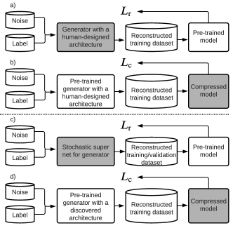
Figure 1: The comparison between the current reconstruction method and the AutoReCon method for data-free compression. The goal of every subfigure is to update the models in gray color, given the pre-trained and fixed models in white color. a) an overview of the current reconstruction method to update the generator by minimizing the reconstruction loss $L_{r}$, where the generator has a human-designed architecture. b) an overview of the current reconstruction for data-free compression to update the compressed model by minimizing the compression loss $L_{c}$, after the generator with the human-designed architecture has been trained in subfigure a). c) an overview of the AutoReCon method to update the generator by minimizing $L_{r}$, where there is a super net for the generator. d) an overview of the AutoReCon method for data-free compression to update the compressed model by minimizing $L_{c}$, after the generator with a discovered architecture has been trained in subfigure c).

3.1 Definition of Reconstruction Method

The pre-trained model $M_{p}$ is obtained by training on the original training dataset $T_{o}=\left\{x_{o},y_{o}\right\}$. Given the pre-trained model $M_{p}$, we compute the reconstructed training dataset $T_{r}=\left\{x_{r},y_{r}\right\}$ with the reconstruction method $\Phi$, i.e., $T_{r}=\Phi(M_{p})$.

Considering the reconstruction method with a generator as shown in Figure 1a), the pre-trained model $M_{p}$ is fixed while the weights of the generator are updated by minimizing the reconstruction loss $L_{r}$. The prior information extracted from the pre-trained model $M_{p}$ by the current methods is mainly the class boundary information and distribution information. If more prior information can be extracted from the pre-trained model, the reconstruction method can be easily adjusted by incorporating more loss terms to the reconstruction loss. Current reconstruction method $\Phi$ can be expressed as follows.

$$\begin{split}&\operatorname*{min}_{W_{g}}L_{r}(W_{g})=\operatorname*{min}_{W_{g}}\operatorname{\mathbb{E}}_{y_{o}\sim{{P_{y_{o}}(y_{o})}},z\sim P_{z}(z)}\\ &[L_{class}(M_{p}(M_{g}(z|y_{o});W_{g}),y_{o})+L_{bns}(BN_{r},BN_{o})]\end{split}$$ (1)

where $z$ and $W_{g}$ are the random noise input vector and weights of the generator, and $L_{class}(\cdot,\cdot)$ is the cross-entropy loss function. $L_{bns}(\cdot,\cdot)$ measures the distribution distance between the batch normalization statistics of the original training dataset $BN_{o}$ and the batch normalization statistics of the reconstructed training dataset $BN_{r}$. The formulations of $L_{class}$, $L_{bns}$, and $L_{r}$ are flexible to make the AutoReCon method general.

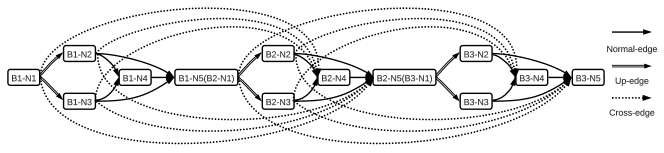
Figure 2: The macro-architecture for the generator. The macro-architecture is a directed acyclic graph consisting of an ordered sequence of nodes. For example, the rectangle with the tag ”B1-N1” represents the $1^{\text{st}}$ node of the $1^{\text{st}}$ convolutional block. ”B1-N5(B2-N1)” indicates the $5^{th}$ node of the $1^{\text{st}}$ convolutional block is the same as the $1^{\text{st}}$ node of the $2^{\text{nd}}$ convolutional block.

3.2 AutoReCon Method

As shown in Figure 1a) and c), we present an overview of current reconstruction and the AutoReCon method. The current reconstruction method includes a pre-trained model $M_{p}$ and a generator $M_{g}$ with a human-designed architecture. In the AutoReCon method, we aim to search for a superior generator architecture automatically for reconstruction.

Regarding the reconstruction task, our training objective function is written as follows, where both weights $W_{g}$ and architecture $A_{g}$ of the generator can be updated by minimizing the reconstruction loss.

$$\begin{split}&\operatorname*{min}_{A_{g}}L_{r}^{\text{val}}(A_{g},W_{g}^{*}(A_{g}))\\ &s.t.~{}W_{g}^{*}(A_{g})=\operatorname*{argmin}_{W_{g}}~{}L_{r}^{\text{train}}(A_{g},W_{g})\end{split}$$ (2)

where $L_{r}^{\text{train}}$ and $L_{r}^{\text{val}}$ refer to the reconstruction loss function on the reconstructed training dataset and the reconstructed validation dataset, respectively. $W_{g}^{*}(A_{g})$ are the optimal weights of the generator given the generator architecture $A_{g}$. $A_{g}\in S$ and $S$ is the whole search space of the generator.

3.2.1 The Search Space

We construct a layer-wise search space with a fixed macro-architecture for the generator. The macro-architecture defines the type of the edge, the number of edges, the node connection, and the input/output dimension of each node. The macro-architecture is shown in Figure 2, where there are three convolutional blocks and five nodes in every convolutional block. We denote the generator as $M_{g}(e_{1},...,e_{i},...,e_{E})$, where $e_{i}$ represents the $i^{th}$ edge and $E$ is the number of edges. The nodes refer to the feature maps and we calculate them as the summation of the outputs of their previous connected edges. There are three types of edges: normal-edge, up-edge, and cross-edge. Normal-edge connects two nodes with the same dimension. Up-edge is used to increase the spatial resolution. Normal-edge and Up-edge are within a convolutional block. Cross-edge connects two adjacent convolutional blocks.

Edge type	Mixture of candidate operations
Normal-edge	Convolution 1 $\times$ 1, dilation=1
	Convolution 3 $\times$ 3, dilation=1
	Convolution 5 $\times$ 5, dilation=1
	Convolution 3 $\times$ 3, dilation=2
	Convolution 5 $\times$ 5, dilation=2
	Identity
	None
Up-edge	Nearest Neighbor Interpolation
	Bilinear Interpolation
Cross-edge	Nearest Neighbor Interpolation
	Bilinear Interpolation
	None

Table 1: For different types of edges, there are different mixtures of candidate operations.

To construct a layer-wise search space for the generator, we set each edge as a mixture of candidate operations, which has several parallel operations instead of one specific operation. Thus, the over-parameterized generator is expressed as $M_{g}(e_{1}=C_{1},...,e_{i}=C_{i},...,e_{E}=C_{E})$ and $C_{i}$ is the mixture of candidate operations for the edge $e_{i}$. As shown in Table 1, different types of edges use different mixtures of candidate operations. Taking the edge $C_{i}$ as an example, we compute its output by summing the outputs of the mixture of candidate operations as follows.

$$X_{out}^{i}=C_{i}(X_{in}^{i})=\sum_{j=1}^{F}O_{j}^{i}(X_{in}^{i})$$ (3)

where $X_{in}^{i}$ and $X_{out}^{i}$ are the input and output of the $i^{th}$ edge. $O_{j}^{i}$ denotes the $j^{th}$ candidate operation of the $i^{th}$ edge and $j=1,...,F$. $F$ is the number of candidate operations for an edge.

3.2.2 The Search Algorithm

The search algorithm represents the search space as a stochastic super net $M_{s}$. In the stochastic super net $M_{s}$, $O_{j}^{i}$ is associated with an architecture parameter $\alpha_{j}^{i}$. To derive a generator $A_{g}$ from the stochastic super net $M_{s}$, the candidate operation $O_{j}^{i}$ is sampled with the probability $p_{j}^{i}$, which is computed as follows.

$$p_{j}^{i}(O_{j}^{i};\alpha^{i})=\text{softmax}(\alpha^{i})=\frac{exp(\alpha_{j}^{i})}{\sum_{j=1}^{F}exp(\alpha_{j}^{i})}$$ (4)

Since sampling from the mixture of candidate operations for each edge is independent, the probability of sampling a generator architecture $A_{g}$ can be described as follows.

$$P(A_{g};\alpha_{g})=\prod_{i=1}^{E}p_{j}^{i}(O_{j}^{i};\alpha^{i})$$ (5)

In this case, we can approximate the problem of finding an optimized discrete generator architecture by finding optimized sampling probabilities. The training objective function of the AutoReCon method is re-written from Equation 2 as follows.

$$\begin{split}&\operatorname*{min}_{a_{g}}\operatorname{\mathbb{E}}_{a_{g}\sim P_{a_{g}}(a_{g})}[L_{r}^{\text{val}}(a_{g},W_{g}^{*}(a_{g}))]\\ &s.t.~{}W_{g}^{*}(a_{g})=\operatorname*{argmin}_{W_{g}}~{}L_{r}^{\text{train}}(a_{g},W_{g})\end{split}$$ (6)

To make the reconstruction loss differentiable to the sampling probabilities, we compute continuous variables $m_{j}^{i}$ by the Gumbel Softmax function as an alternative as follows.

$$m_{j}^{i}=\text{GumbelSoftmax}(p^{i})=\frac{exp\left[(p_{j}^{i}+g_{j}^{i})/\tau\right]}{\sum_{j=1}^{F}exp\left[(p_{j}^{i}+g_{j}^{i})/\tau\right]}$$ (7)

where $g_{j}^{i}$ is the noise sampled from the Gumbel distribution ($0,1$) and $\tau$ is a temperature parameter to control the sampling operation. Then, the continuous variables $m_{j}^{i}$ are directly differentiable with respect to the sampling probabilities. Thus, the computation of the edge $C_{i}$ in Equation 3 can be expressed as follows.

$$X_{out}^{i}=C_{i}(X_{in}^{i})=\sum_{j=1}^{F}m_{j}^{i}O_{j}^{i}(X_{in}^{i})$$ (8)

Algorithm 1 The AutoReConmethod for data-free compression

0:  Pre-trained model $M_{p}$.

0:  Discovered generator $M_{g}$, compressed model $M_{c}$. Stage 1: Searching for generator architecture.

1:  for $epoch=1$ to $L_{1}$ do

2:     for $batch=1$ to $T_{1}$ do

3:        Obtain random noise $z\sim N(0,1)$ and label $y_{o}$. Generate reconstructed training dataset $T_{r}$ with stochastic super net $M_{s}$. Update weights of stochastic super net by minimizing reconstruction loss $L_{r}$.

4:     end for

5:     for $batch=1$ to $V_{1}$ do

6:        Obtain random noise $z\sim N(0,1)$ and label $y_{o}$. Generate reconstructed validation dataset $V_{r}$ with stochastic super net $M_{s}$. Update architecture parameters of stochastic super net by minimizing reconstruction loss $L_{r}$.

7:     end for

8:  end forStage 2: Compression with discovered generator.

9:  for $epoch=1$ to $L_{2}$ do

10:     for $batch=1$ to $T_{2}$ do

11:        Obtain random noise $z\sim N(0,1)$ and label $y_{o}$. Generate reconstructed training dataset $T_{r}$ with the discovered generator $M_{g}$. Update weights of compressed model $M_{c}$ by minimizing compression loss $L_{c}$.

12:     end for

13:  end for

3.3 Training Process

Using the AutoReCon method, the training process for data-free compression is illustrated as shown in Algorithm 1. The first stage of the training process is to search for generator architecture with our AutoReCon method, as shown in Figure 1c). The goal of the first stage is to seek an optimized generator architecture from the stochastic super net. The second stage of the training process is to compress the pre-trained model $M_{p}$ with the discovered generator $M_{g}$. The compression loss $L_{c}$ can be introduced from quantization and/or knowledge distillation. Compared with the current reconstruction methods, our AutoReCon method considers network engineering and search for an optimized generator architecture for reconstruction.

Method	Pre-trained model	Generator	Quantization	Top-1(CIFAR-100)	Top-1(ImageNet)
-	ResNet18	-	-	$78.83\%$	-
-	ResNet18	-	-	-	$71.47\%$
GDFQ	ResNet18	Human-designed	w6a6	$78.00\%$	$70.10\%$
GDFQ	ResNet18	Human-designed	w5a5	$75.93\%$	$68.38\%$
GDFQ	ResNet18	Human-designed	w4a4	$60.23\%$	$60.70\%$
GDFQ	ResNet18	Human-designed	w3a3	$28.71\%$	$20.69\%$
Ours	ResNet18	Discovered by AutoReCon	w6a6	$78.52\%$($+0.52\%$)	$70.61\%$($+0.51\%$)
Ours	ResNet18	Discovered by AutoReCon	w5a5	$77.22\%$($+1.29\%$)	$68.88\%$($+0.50\%$)
Ours	ResNet18	Discovered by AutoReCon	w4a4	$71.02\%$($+10.79\%$)	$61.32\%$($+0.62\%$)
Ours	ResNet18	Discovered by AutoReCon	w3a3	$46.44\%$($+17.73\%$)	$23.37\%$($+2.68\%$)
-	MobileNetV2	-	-	$70.72\%$	-
-	MobileNetV2	-	-	-	$73.03\%$
GDFQ	MobileNetV2	Human-designed	w6a6	$69.59\%$	$71.18\%$
GDFQ	MobileNetV2	Human-designed	w5a5	$65.27\%$	$67.81\%$
GDFQ	MobileNetV2	Human-designed	w4a4	$53.91\%$	$59.80\%$
GDFQ	MobileNetV2	Human-designed	w3a3	$8.50\%$	$2.31\%$
Ours	MobileNetV2	Discovered by AutoReCon	w6a6	$70.57\%$($+0.98\%$)	$71.53\%$($+0.33\%$)
Ours	MobileNetV2	Discovered by AutoReCon	w5a5	$67.95\%$($+2.68\%$)	$68.40\%$($+0.59\%$)
Ours	MobileNetV2	Discovered by AutoReCon	w4a4	$58.42\%$($+4.51\%$)	$60.13\%$($+0.33\%$)
Ours	MobileNetV2	Discovered by AutoReCon	w3a3	$10.21\%$($+1.71\%$)	$14.30\%$($+11.99\%$)
-	ResNet50	-	-	$79.36\%$	-
-	ResNet50	-	-	-	$77.72\%$
GDFQ	ResNet50	Human-designed	w6a6	$78.79\%$	$76.40\%$
GDFQ	ResNet50	Human-designed	w5a5	$76.17\%$	$70.79\%$
GDFQ	ResNet50	Human-designed	w4a4	$61.44\%$	$55.94\%$
GDFQ	ResNet50	Human-designed	w3a3	$26.51\%$	$1.20\%$
Ours	ResNet50	Discovered by AutoReCon	w6a6	$79.12\%$($+0.33\%$)	$76.76\%$($+0.36\%$)
Ours	ResNet50	Discovered by AutoReCon	w5a5	$77.06\%$($+0.89\%$)	$74.13\%$($+3.34\%$)
Ours	ResNet50	Discovered by AutoReCon	w4a4	$68.20\%$($+6.76\%$)	$64.37\%$($+8.43\%$)
Ours	ResNet50	Discovered by AutoReCon	w3a3	$36.17\%$($+9.66\%$)	$1.63\%$($+0.43\%$)

Table 2: Experimental results of data-free compression on CIFAR-100 and ImageNet classification. $w4a4$ means that the weights and activations are quantized to $4$-bit precision. Both our data-free compression method and the GDFQ adopt knowledge distillation for the output layer. In each block, the first row presents the accuracy of the full-precision pre-trained model on CIFAR-100. The second row shows the accuracy of the full-precision pre-trained model on ImageNet.

4 Experiments

4.1 Implementation Details

Our interest is to show the performance improvement of data-free compression, which is brought by the AutoReCon method. We adopt the GDFQ data-free compression method Xu et al. (2020) as a baseline for the following three reasons. First, it exploits both class boundary information and distribution information from the pre-trained model $M_{p}$, compared to other methods that use only one type of information Cai et al. (2020); Yoo et al. (2019); Chen et al. (2019); Nayak et al. (2019). Second, it includes both data-free quantization and data-free knowledge distillation, where knowledge distillation is applied for the output layer (i.e., knowledge distillation is not applied for the intermediate layers). Third, it achieves state-of-the-art performance. We use the same experimental settings as the GDFQ method to observe the influence of the generator architecture. In the GDFQ method, the human-designed generator architecture for both CIFAR-100 and ImageNet classification follows ACGAN. Besides, the human-designed generator for ImageNet classification adopts the categorical conditional batch normalization layer to fuse label information following SN-GAN.

4.2 Results on Image Classification

4.2.1 Results on ImageNet Classification

As shown in Table 2, we report the experimental results of data-free compression on the ImageNet classification dataset. Replacing the human-designed generator with the generator discovered by our AutoReCon method, the accuracy of the GDFQ method increases consistently using different pre-trained models and low-bit width quantization. Using ResNet18 as the pre-trained model and $3$-bit width quantization, the Top-1 accuracy of the GDFQ method can increase by $2.68\%$ when using the generator discovered by the AutoReCon method. The Top-1 accuracy of the GDFQ method increases by $11.99\%$ using MobileNetV2 as the pre-trained model, $3$-bit width quantization, and the generator discovered by the AutoReCon method. Using ResNet50 as the pre-trained model and $5$-bit width quantization, the Top-1 accuracy of our data-free compression with an optimized generator surpasses the GDFQ method by $8.43\%$. In addition, the optimized generator needs almost the same parameters and fewer flops compared with a human-designed generator.

4.2.2 Results on CIFAR-100 Classification

As shown in Table 2, we report the experimental results of data-free compression on the CIFAR-100 classification dataset. Using various pre-trained models and low-bit width quantization, our data-free compression with an optimized generator architecture achieves better accuracy than the GDFQ method with a human-designed generator. Using ResNet18 as the pre-trained model and $3$-bit width quantization, the Top-1 accuracy of the GDFQ method will improve by $17.73\%$ if the human-designed generator is replaced with the generator discovered by the AutoReCon method. Using MobileNetV2 and $5$-bit width quantization, the Top-1 accuracy of our data-free compression shows an improvement of $4.51\%$ compared with the GDFQ method. The Top-1 accuracy improvement becomes $9.66\%$ using ResNet50 as the pre-trained model and $4$-bit width quantization.

4.3 Ablation Study

Method	Scale	Top-1	Top-5
GDFQ	$s=4$	$64.87\%$	$86.76\%$
GDFQ	$s=3$	$65.04\%$	$86.93\%$
GDFQ	$s=2$	$65.22\%$	$87.19\%$
GDFQ	$s=1$	$65.27\%$	$87.30\%$
GDFQ	$s=0.5$	$63.72\%$	$86.21\%$
Ours	$s=4$	$68.78\%$($+3.91\%$)	$88.62\%$
Ours	$s=3$	$68.09\%$($+3.05\%$)	$89.01\%$
Ours	$s=2$	$67.95\%$($+2.73\%$)	$88.76\%$
Ours	$s=1$	$67.58\%$($+2.31\%$)	$88.42\%$
Ours	$s=0.5$	$66.30\%$($+2.58\%$)	$88.09\%$

Table 3: Experimental results of data-free compression on CIFAR-100 classification. The GDFQ method uses a human-designed generator. Our data-free compression uses the generator discovered by the AutoRe method.

4.3.1 Scalability of Discovered Generator Architectures

We explore the scalability of the discovered generator architecture for data-free compression on the CIFAR-100 classification dataset. We scale the base channels by a factor from $s=0.5$ to $s=4$ for the discovered generator and the human-designed generator. The data-free compression results using MobileNetV2 as the pre-trained model, $5$-bit width quantization, and knowledge distillation applied for the output layer are shown in Table 3. Without modifying the optimized generator architecture, the performance of our data-free compression keeps increasing and is always better than the GDFQ method when scaling the base channels by the factor from $s=0.5$ to $4.0$. The accuracy of the GDFQ method decreases when we scale the base channels for the human-designed generator. Thus, we conclude that our searched generator architecture has superior scalability compared to the human-designed generator for data-free compression.

Method	Generator	Top-1
-	-	$77.50\%$
DAFL	Human-designed	$61.40\%$
DFAD	Human-designed	$67.70\%$
Ours	Discovered by AutoReCon	$69.98\%$($+2.28\%$)

Table 4: Experimental results of data-free compression on CIFAR-100 classification. The first row is the accuracy of the pre-trained teacher model.

4.3.2 Generalization of AutoReCon Method

Except for the GDFQ method, we use the GFADFang et al. (2019) method as a baseline to show the generalization of our AutoReCon method. The generation loss in the GFAD method is replaced with the reconstruction loss of Equation 6, which enables the exploration of generator architecture. We use ResNet34 as the pre-trained teacher model and ResNet18 as the student model. The experimental results of data-free knowledge distillation on CIFAR-100 is shown in Table 4. With a human-designed generator, the GFAD method achieves better accuracy than the DAFLChen et al. (2019) method. The Top-1 accuracy of our data-free knowledge distillation with a discovered generator is $2.28\%$ better than the baseline of the GFAD method with a human-designed generator.

Method	Pre-trained model	Quantization	Top-1
-	ResNet18	-	$71.47\%$
DFQ	ResNet18	w4a4	$0.10\%$
ZeroQ	ResNet18	w4a4	$26.04\%$
DFC	ResNet18	w4a4	$55.49\%$
GDFQ	ResNet18	w4a4	$60.70\%$
Ours	ResNet18	w4a4	$61.60\%$
-	MobileNetV2	-	$73.03\%$
DFQ	MobileNetV2	w4a4	$0.11\%$
ZeroQ	MobileNetV2	w4a4	$3.31\%$
GDFQ	MobileNetV2	w4a4	$59.80\%$
Ours	MobileNetV2	w4a4	$60.02\%$
-	ResNet50	-	$77.72\%$
ZeroQ	ResNet50	w4a4	$0.12\%$
GDFQ	ResNet50	w4a4	$55.94\%$
Ours	ResNet50	w4a4	$57.49\%$

Table 5: Comparison of different data-free compression methods on ImageNet classification. $w4a4$ means that the weights and activations are quantized to $4$-bit precision. The first row of each block is the accuracy of the full-precision pre-trained model.

4.4 Comparison with State-of-the-art Methods

On the ImageNet classification dataset, we present the results of additional data-free compression methods as shown in Table 5. The comparison is mainly for data-free quantization except that the GDFQ and our methods apply knowledge distillation on the output layer. None of the compared methods apply knowledge distillation on the intermediate layers. The results of DFQ Nagel et al. (2019) and ZeroQ Cai et al. (2020) are cited from the GDFQ paper and have a rather low accuracy for ultra-low precision data-free quantization. The DFC Haroush et al. (2020) method achieves a moderate accuracy with a combination of BN-Statistics and Inception schemes. Our method achieves better accuracy compared to the GDFQ method since the AutoReCon method discovers an optimized generator architecture for reconstruction.

5 Conclusion

In this paper, we present the AutoReCon method, which is the first work to consider network engineering of the reconstruction method to improve the performance of data-free compression. In particular, our AutoReCon method can search for an optimized generator architecture from a stochastic super net with gradient-based neural architecture search for reconstruction. When we plug our discovered generator to replace the human-designed generator, our data-free compression benefits from the optimization of the generator architecture and achieves better accuracy. Specifically, using ResNet50 as the pre-trained model and $5$-bit width quantization, the Top-1 accuracy of our data-free compression on ImageNet with an optimized generator surpasses the GDFQ method by $8.43\%$. The Top-1 accuracy of the DFAD method on CIFAR-100 increases by $2.28\%$ using ResNet34 as the pre-trained teacher model, ResNet18 as the student model, and the generator discovered by the AutoReCon method.

References

- Banner et al. [2018] Ron Banner, Yury Nahshan, Elad Hoffer, and Daniel Soudry. Aciq: analytical clipping for integer quantization of neural networks. arXiv preprint arXiv:1810.05723, 2018, 2018.
- Cai et al. [2020] Yaohui Cai, Zhewei Yao, Zhen Dong, Amir Gholami, Michael W Mahoney, and Kurt Keutzer. Zeroq: A novel zero shot quantization framework. In Proceedings of the IEEE/CVF Conference on Computer Vision and Pattern Recognition, pages 13169–13178, 2020.
- Chen et al. [2018] Liang-Chieh Chen, Maxwell Collins, Yukun Zhu, George Papandreou, Barret Zoph, Florian Schroff, Hartwig Adam, and Jon Shlens. Searching for efficient multi-scale architectures for dense image prediction. In Advances in neural information processing systems, pages 8699–8710, 2018.
- Chen et al. [2019] Hanting Chen, Yunhe Wang, Chang Xu, Zhaohui Yang, Chuanjian Liu, Boxin Shi, Chunjing Xu, Chao Xu, and Qi Tian. Data-free learning of student networks. In Proceedings of the IEEE International Conference on Computer Vision, pages 3514–3522, 2019.
- Choi et al. [2020] Yoojin Choi, Jihwan Choi, Mostafa El-Khamy, and Jungwon Lee. Data-free network quantization with adversarial knowledge distillation. In Proceedings of the IEEE/CVF Conference on Computer Vision and Pattern Recognition Workshops, pages 710–711, 2020.
- Fang et al. [2019] Gongfan Fang, Jie Song, Chengchao Shen, Xinchao Wang, Da Chen, and Mingli Song. Data-free adversarial distillation. arXiv preprint arXiv:1912.11006, 2019.
- Gao et al. [2020] Chen Gao, Yunpeng Chen, Si Liu, Zhenxiong Tan, and Shuicheng Yan. Adversarialnas: Adversarial neural architecture search for gans. In Proceedings of the IEEE/CVF Conference on Computer Vision and Pattern Recognition, pages 5680–5689, 2020.
- Haroush et al. [2020] Matan Haroush, Itay Hubara, Elad Hoffer, and Daniel Soudry. The knowledge within: Methods for data-free model compression. In Proceedings of the IEEE/CVF Conference on Computer Vision and Pattern Recognition, pages 8494–8502, 2020.
- He et al. [2020] Yang He, Yuhang Ding, Ping Liu, Linchao Zhu, Hanwang Zhang, and Yi Yang. Learning filter pruning criteria for deep convolutional neural networks acceleration. In Proceedings of the IEEE/CVF Conference on Computer Vision and Pattern Recognition, pages 2009–2018, 2020.
- Howard et al. [2019] Andrew Howard, Mark Sandler, Grace Chu, Liang-Chieh Chen, Bo Chen, Mingxing Tan, Weijun Wang, Yukun Zhu, Ruoming Pang, Vijay Vasudevan, et al. Searching for mobilenetv3. In Proceedings of the IEEE International Conference on Computer Vision, pages 1314–1324, 2019.
- Liu et al. [2018] Hanxiao Liu, Karen Simonyan, and Yiming Yang. Darts: Differentiable architecture search. arXiv preprint arXiv:1806.09055, 2018.
- Lopes et al. [2017] Raphael Gontijo Lopes, Stefano Fenu, and Thad Starner. Data-free knowledge distillation for deep neural networks. arXiv preprint arXiv:1710.07535, 2017.
- Mehta et al. [2019] Sachin Mehta, Mohammad Rastegari, Linda Shapiro, and Hannaneh Hajishirzi. Espnetv2: A light-weight, power efficient, and general purpose convolutional neural network. In Proceedings of the IEEE conference on computer vision and pattern recognition, pages 9190–9200, 2019.
- Micaelli and Storkey [2019] Paul Micaelli and Amos J Storkey. Zero-shot knowledge transfer via adversarial belief matching. In Advances in Neural Information Processing Systems, pages 9551–9561, 2019.
- Mirzadeh et al. [2020] Seyed Iman Mirzadeh, Mehrdad Farajtabar, Ang Li, Nir Levine, Akihiro Matsukawa, and Hassan Ghasemzadeh. Improved knowledge distillation via teacher assistant. In Proceedings of the AAAI Conference on Artificial Intelligence, pages 5191–5198, 2020.
- Nagel et al. [2019] Markus Nagel, Mart van Baalen, Tijmen Blankevoort, and Max Welling. Data-free quantization through weight equalization and bias correction. In Proceedings of the IEEE International Conference on Computer Vision, pages 1325–1334, 2019.
- Nayak et al. [2019] Gaurav Kumar Nayak, Konda Reddy Mopuri, Vaisakh Shaj, R Venkatesh Babu, and Anirban Chakraborty. Zero-shot knowledge distillation in deep networks. arXiv preprint arXiv:1905.08114, 2019.
- Pham et al. [2018] Hieu Pham, Melody Y Guan, Barret Zoph, Quoc V Le, and Jeff Dean. Efficient neural architecture search via parameter sharing. arXiv preprint arXiv:1802.03268, 2018.
- Xu et al. [2020] Shoukai Xu, Haokun Li, Bohan Zhuang, Jing Liu, Jiezhang Cao, Chuangrun Liang, and Mingkui Tan. Generative low-bitwidth data free quantization. arXiv preprint arXiv:2003.03603, 2020.
- Yin et al. [2020] Hongxu Yin, Pavlo Molchanov, Jose M Alvarez, Zhizhong Li, Arun Mallya, Derek Hoiem, Niraj K Jha, and Jan Kautz. Dreaming to distill: Data-free knowledge transfer via deepinversion. In Proceedings of the IEEE/CVF Conference on Computer Vision and Pattern Recognition, pages 8715–8724, 2020.
- Yoo et al. [2019] Jaemin Yoo, Minyong Cho, Taebum Kim, and U Kang. Knowledge extraction with no observable data. In Advances in Neural Information Processing Systems, pages 2705–2714, 2019.
- Zhu et al. [2020a] Baozhou Zhu, Zaid Al-Ars, and H Peter Hofstee. Nasb: Neural architecture search for binary convolutional neural networks. In 2020 International Joint Conference on Neural Networks (IJCNN), pages 1–8. IEEE, 2020.
- Zhu et al. [2020b] Baozhou Zhu, Zaid Al-Ars, and Wei Pan. Towards lossless binary convolutional neural networks using piecewise approximation. In European Conference on Artificial Intelligence (ECAI), 2020.