Density estimation on low-dimensional manifolds: an inflation-deflation approach

Abstract

Normalizing Flows (NFs) are universal density estimators based on Neural Networks. However, this universality is limited: the density’s support needs to be diffeomorphic to a Euclidean space. In this paper, we propose a novel method to overcome this limitation without sacrificing universality. The proposed method inflates the data manifold by adding noise in the normal space, trains an NF on this inflated manifold, and, finally, deflates the learned density. Our main result provides sufficient conditions on the manifold and the specific choice of noise under which the corresponding estimator is exact. Our method has the same computational complexity as NFs and does not require computing an inverse flow. We also show that, if the embedding dimension is much larger than the manifold dimension, noise in the normal space can be well approximated by Gaussian noise. This allows using our method for approximating arbitrary densities on unknown manifolds provided that the manifold dimension is known.

Keywords: Normalizing Flow, Density Estimation, low-dimensional manifolds, normal space, noise

1 Introduction

Many modern problems involving high-dimensional data are formulated probabilistically. Key concepts, such as Bayesian Classification, Denoising, or Anomaly Detection, rely on the data generating density $p^{*}(x)$. Therefore, a main research area and of crucial importance is learning this data generating density $p^{*}(x)$ from samples.

For the case where the corresponding random variable $X$ with values in $\mathbb{R}^{D}$ takes values on a manifold diffeomorphic to $\mathbb{R}^{D}$, a Normalizing Flow (NF) can be used to learn $p^{*}(x)$ exactly (Huang et al. (2018)). However, in practice, many real-world applications such as predicting protein structures in molecular biology (Hamelryck et al. (2006)), learning motions in robotics (Feiten et al. (2013)), or predicting earthquake patterns in geology (Geller (1997)) are modeled on low-dimensional manifolds, and therefore gave rise to the manifold hypothesis which states that high-dimensional datasets, such as high-resolution images, live close to a low-dimensional manifold (see Fefferman et al. (2016) and the references therein). As a consequence, few attempts have been made to use NFs to learn densities on low-dimensional manifolds, overcoming their topological constraint. To do so, these methods either need to know the manifold beforehand (Gemici et al. (2016), Rezende et al. (2020), Mathieu and Nickel (2020), Lou et al. (2020)), or sacrifice the directness of the estimate (Beitler et al. (2018), Kim et al. (2020), Cunningham et al. (2020), Brehmer and Cranmer (2020)).

Our goal in this paper is to overcome both the aforementioned limitations of using NFs for density estimation on Riemannian manifolds. Given data points from a $d-$dimensional Riemannian manifold denoted as $\mathcal{X}$ embedded in $\mathbb{R}^{D}$, $d<D$, we first inflate the manifold by adding a specific noise in the normal space direction of the manifold, then train an NF on this inflated manifold, and, finally, deflate the trained density by exploiting the choice of noise and the geometry of the manifold. See Figure 1 for a schematic overview of these points.

Figure 1: Schematic overview of our method. 1. A density $p^{*}(x)$ with support on a $d$-dimensional manifold $\mathcal{X}$ (top left) is inflated by adding noise $\sigma^{2}$ in the normal space (top right). 2. We have an NF $F^{-1}_{\theta}(x)$ learn this inflated density $q(\tilde{x})$ using a well-known reference measure $p_{\mathcal{U}}(u)$. 3. We deflate the learned density to obtain an estimate $\hat{p}(x)$ for $p^{*}(x)$. 4. Our main result provides sufficient conditions for the manifold $\mathcal{X}$ and the choice of noise such that $\hat{p}(x)=p^{*}(x)$.

Our main theorem states sufficient conditions on the manifold and the type of noise we use for the inflation step such that the deflation becomes exact. To guarantee the exactness, we do need to know the manifold as in e.g. Rezende et al. (2020) because we need to be able to sample in the manifold’s normal space. However, as we will show, for the special case where $D\gg d$, the usual Gaussian noise approximates a Gaussian restricted to the normal space. This allows using our method for approximating arbitrary densities on Riemannian manifolds provided that the manifold dimension is known. In addition, our method is based on a single NF without the necessity to invert it. Hence, we don’t add any additional complexity to the training procedure of NFs such that autoregressive flows (which are typically $D$-times slower to invert) can be used. To the best of our knowledge, this is the first theoretical study that provides sufficient conditions for the learnability of a density with support on a low-dimensional manifold using NFs.

Notations: We denote the Lebesgue measure in $\mathbb{R}^{n}$ as $\lambda_{n}$. Random variables will be denoted with a capital letter, e.g. $X$, and their corresponding state spaces with the calligraphic version, $\mathcal{X}$. Small letters correspond to vectors with dimensionality given by context. The letters $d,D,n$, and $N$ are always natural numbers.

2 Background and problem statement

Let $X$ be a random variable that takes values on a $d-$dimensional manifold $\mathcal{X}$ embedded in $\mathbb{R}^{D}$, i.e $\mathcal{X}\subset\mathbb{R}^{D}$, and let $X$ be generated by an unobserved random variable $U\in\mathcal{U}\subset\mathbb{R}^{d}$ with density $\pi_{u}(u)$, where $d<D$. That is, from a generative perspective, a sample $x$ from the random variable $X$ is obtained in the following way:

1. sampling from the prior: $u\sim\pi_{u}(u)$,

2. mapping to the manifold: $x=f(u)$.

If $f:\mathcal{U}\to\mathcal{X}$ is an embedding (as it is the case in Gemici et al. (2016)) the density $p^{*}(x)$ of $X$ is given by the change of variable formula

$$p^{*}(x)=\left|\det G_{f}(x)\right|^{-\frac{1}{2}}\pi_{u}(f^{-1}(x)),$$ (1)

where we denote the Gram matrix of $f$ evaluated at $f^{-1}(x)$ as

$$G_{f}(x):=J_{f}(f^{-1}(x))^{T}J_{f}(f^{-1}(x))$$ (2)

with $J_{f}^{T}$ denoting the transpose of the Jacobian of $f$. Hence, given an explicit chart $f$ and samples from $p^{*}(x)$, we can learn the unknown density $\pi_{u}(u)$ using a standard NF in $\mathbb{R}^{d}$. However, in general, the generating function $f$ is either unknown or not an embedding creating numerical instabilities for training inputs close to singularity points.

In Brehmer and Cranmer (2020), $f$ and the unknown density $\pi_{u}$ are learned simultaneously. Their main idea is to define $f$ as a level set of a usual flow in $\mathbb{R}^{D}$ and train it together with the flow in $\mathbb{R}^{d}$ used to learn $\pi_{u}$. To evaluate the density, one needs to calculate $\left|\det G_{f}(x)\right|^{-\frac{1}{2}}$ which computational complexity is $\mathcal{O}(d^{2}D)+\mathcal{O}(d^{3})$. Thus this approach may be slow for high-dimensional data (which we will confirm in Section 5.4). Besides, to guarantee that $f$ learns the manifold they proposed several ad hoc training strategies. We tie in with the idea to use an NF for learning $p^{*}(x)$ with unknown $f$ and study the following problem.

Problem 1

Let $\mathcal{X}$ be a $d-$dimensional manifold embedded in $\mathbb{R}^{D}$. Let $X$ be a random variable with values in $\mathcal{X}$. Given $N$ samples from $p^{*}(x)$ as described above, find an estimator $\hat{p}$ of $p^{*}$ such that in the limit of infinitely many samples we have that $\hat{p}(x)=p^{*}(x)$, $\mathbb{P}_{X}$-almost surely.

The universality of standard NFs: Formally, a standard NF is a diffeomorphism $F_{\theta}:\mathcal{Z}\subseteq\mathbb{R}^{D}\to\mathcal{X}\subseteq\mathbb{R}^{D}$ and induces a density on $\mathcal{X}$ through $p_{\theta}(x)=\left|\det G_{F_{\theta}}(x))\right|^{-\frac{1}{2}}p_{\mathcal{Z}}(F_{\theta}^{-1}(x))$ where $p_{\mathcal{Z}}$ is a known density. The parameters $\theta$ are updated such that the KL-divergence between $p^{*}(x)$ and $p_{\theta}(x)$,

$$D_{KL}(p^{*}(x)||p_{\theta}(x))=-\mathbb{E}_{x\sim p^{*}(x)}[\log p_{\theta}(x)]+const.$$ (3)

is minimized. For certain flow architectures, $F_{\theta}$ is expressive enough such that in the limit of infinitely hidden layers $n$, every $p^{*}(x)$ with support on $\mathbb{R}^{D}$ can be learned exactly, see Huang et al. (2018, 2020) for a rigorous mathematical description. However, this universality depends on the architecture and is not true for all flow types, see Zhang et al. (2020).

Remark 2

1. Note that $p^{*}(x)$ is uniquely determined by the pair $(\pi,f)$. For another embedding $f^{\prime}=f\circ\phi$ with $\phi$ being a diffeomorphism , the pair $(\pi^{\prime},f^{\prime})$ with $\pi^{\prime}=\pi\circ\phi^{-1}$ induces the same density $p^{*}(x)$. Hence, $p^{*}(x)$ does not depend on the specific embedding.

2. The density $p^{*}(x)$ is with respect to the volume form $dV(x)=\sqrt{\left|\det G_{f}(x)\right|}du$, i.e. one can calculate probabilities such as $\mathbb{P}_{X}(A)$ for measurable $A\subset\mathcal{X}$ as follows: $\mathbb{P}(X\in A)=\int_{f^{-1}(A)}\pi_{u}(u)du=\int_{A}p^{*}(x)dV(x)$. Viewing $p^{*}(x)dV$ as a differential $d-$form, we may say that the volume form $dV$ is induced by the Euclidean metric in $\mathbb{R}^{D}$.

3 Methods

To solve Problem 1, we want to exploit the universality of NFs. We want to inflate $\mathcal{X}$ such that the inflated manifold $\tilde{\mathcal{X}}$ becomes diffeomorphic to a set $\mathcal{U}$ on which a simple density exists. By doing so, this allows us to learn the inflated density $q(\tilde{x}),\tilde{x}\in\mathbb{R}^{D}$, exactly using a single NF, see Section 2. Then, given such an estimator for the modified density, we approximate $p^{*}(x)$ and give sufficient conditions when this approximation is exact.

3.1 The Inflation step

Given a sample $x$ of $X$, if we add some noise $\mathcal{E}\in\mathbb{R}^{D}$ to it, the resulting new random variable $\tilde{X}=X+\mathcal{E}$ has the following density

$$q(\tilde{x})=\int_{\mathcal{X}}q(\tilde{x}|x)d\mathbb{P}_{X}(x),$$ (4)

whee $q(\tilde{x}|x)$ is the noise density. Denote the tangent space in $x$ as $T_{x}$ and the normal space as $N_{x}$. By definition, $N_{x}$ is the orthogonal complement of $T_{x}$. Therefore, we can decompose the noise $\mathcal{E}$ into its tangent and normal component, $\mathcal{E}=\mathcal{E}_{\rm{t}}+\mathcal{E}_{\rm{n}}$. In the following, we consider noise in the normal space only, i.e. $\mathcal{E}_{\rm{t}}=0$, and denote the density of the resulting random variable as $q_{\rm{n}}(\tilde{x})$. The corresponding noise density $q_{\rm{n}}(\tilde{x}|x)$ has mean $x$ and domain $N_{x}$. We denote the support of $q_{\rm{n}}(\cdot|x)$ by $N_{q_{\rm{n}}(\cdot|x)}$. The random variable $\tilde{X}=X+\mathcal{E}_{\rm{n}}$ is now defined on $\widetilde{\mathcal{X}}=\bigcup_{x\in\mathcal{X}}N_{q_{\rm{n}}(\cdot|x)}.$ We want $\widetilde{\mathcal{X}}$ to be diffeomorphic to a set $\mathcal{U}$ on which a known density can be defined.

From a generative perspective, a sample $\tilde{x}$ from the random variable $\widetilde{\mathcal{X}}$ is obtained in the following way:

1. sampling from the prior: $u\sim\pi_{u}(u)$ and $v\sim\pi_{v}(v)$

2. mapping to the inflated manifold: $\tilde{x}_{\rm{n}}=x+A_{u}v$,

where $\pi_{v}$ is the noise generating latent density in $\mathbb{R}^{D-d}$, and $A_{u}\in\mathbb{R}^{D}\times\mathbb{R}^{D-d}$ is the matrix with columns consisting of normal vectors spanning the normal space in $x=f(u)$. Without loss of generality, we can choose an orthonormal basis for $N_{x}$ such that $\det A_{u}^{T}A_{u}=1$.

Example 1

1. Let $\mathcal{X}=S^{1}=\{x\in\mathbb{R}^{2}\ |\ ||x||_{2}=1\}$ be the unit circle where $||\cdot||_{2}$ denotes the $L_{2}-$norm. For each $x\in S^{1}$ there exists $u\in[0,2\pi)$ such that $x=e_{r}(x)=(\cos(u),\sin(u))^{T}$. To sample a point $\tilde{x}$ in $N_{x}$, which is spanned by $e_{r}(x)$, we sample a scalar value $v$ and set $\tilde{x}=x+ve_{r}(x)$. With $V\sim\mathrm{Uniform}[-1,1)$, we have that

   $$\widetilde{\mathcal{X}}=\bigcup_{x\in\mathcal{X}}\{x+ve_{r}(x)|v\in[-1,1)\}=\{x\in\mathbb{R}^{2}\ |\ ||x||_{2}<2\}$$ (5)

   which is the open disk with radius $2$. The open disk is diffeomorphic to $(0,1)\times(0,1)$. Thus, $q_{\rm{n}}(\tilde{x})$ can be learned by a single NF denoted as $F^{-1}$ and $p_{\mathcal{Z}}(u)=\mathrm{Uniform}\left((0,1)\times(0,1)\right)$ as reference.

2. As in (a), we consider the unit circle. Now we set $V$ to be a shifted $\chi^{2}-$ distribution with support $[-1,\infty)$. Then,

   $$\widetilde{\mathcal{X}}=\bigcup_{x\in\mathcal{X}}\{x+ve_{r}(x)|v\in[-1,\infty)\}=\mathbb{R}^{2}.$$ (6)

   Thus, $q_{\rm{n}}(\tilde{x})$ can be learned by a single NF denoted as $F^{-1}$ and $p_{\mathcal{Z}}(z)=\mathcal{N}(z;0,I_{D})$ as reference.

Both cases can be analogously extended to higher dimensions.

3.2 The Deflation step

Equation (4) defines the density of the random variable $\tilde{X}=X+\mathcal{E}$. However, if the noise $\mathcal{E}$ is added in the normal space such that for each realization $\tilde{x}$ there exist only one $x$, we show that

$$q_{\rm{n}}(x)=q_{\rm{n}}(x|x)p^{*}(x).$$ (7)

If the estimator $\hat{q}_{\rm{n}}(\tilde{x})$ is exact, i.e. $\hat{q}_{\rm{n}}(\tilde{x})=q_{\rm{n}}(\tilde{x})$ for $\mathbb{P}_{\tilde{X}}-$almost all $\tilde{x}\in\widetilde{\mathcal{X}}$, we have for $\tilde{x}=x$ that $p^{*}(x)=\hat{q}_{\rm{n}}(x)/q_{\rm{n}}(x|x)$ and therefore $p^{*}(x)$ can be computed from an NF and a known scaling factor.

For equation (7) to be true, we need to guarantee that almost every $\tilde{x}$ corresponds to only one $x\in\mathcal{X}$. This is certainly the case whenever all the normal spaces have no intersections at all (think of a simple line in $\mathbb{R}^{2}$). We can relax this assumption by allowing null-set intersections. Moreover, only those subsets of the normal spaces are of interest which are generated by the specific choice of noise $q_{\rm{n}}(\tilde{x}|x)$. Thus, only the support of $q_{\rm{n}}(\tilde{x}|x)$, denoted by $N_{q_{\rm{n}}(\cdot|x)}$, matters. The key concept for our main result is expressed in the following definition:

Definition 3

Let $\mathcal{X}$ be a $d-$dimensional manifold and $N_{x}$ the normal space in $x\in\mathcal{X}$. Let $q_{\rm{n}}(\cdot|x)$ be a density defined on $N_{x}$ and denote by $N_{q_{\rm{n}}(\cdot|x)}\subseteq N_{x}$. Denote the collection of all such densities as $Q:=\{q_{\rm{n}}(\cdot|x)\}_{x\in\mathcal{X}}$. For $\tilde{x}\in\widetilde{\mathcal{X}}$, we define the set of all possible generators of $\tilde{x}$ as $\mathcal{A}(\tilde{x})=\{x^{\prime}\in\mathcal{X}|N_{q_{\rm{n}}(\cdot|x^{\prime})}\ni\tilde{x}\}$. We say $\mathcal{X}$ is $Q-$normally reachable if for all $x\in\mathcal{X}$, it holds that $\mathbb{P}_{\tilde{X}|X=x}\left(\tilde{x}\in N_{x}|\#\mathcal{A}(\tilde{x})>1\right)=0$ where $\#\mathcal{A}(\tilde{x})$ is the cardinality of the set $\mathcal{A}(\tilde{x})$. In other words, every $\tilde{x}\in N_{x}$ is $\mathbb{P}_{\tilde{X}|X=x}$-almost surely determined by $x$.

To familiarize with this concept, consider Figure 2 and the following example:

Example 2

For the circle in example 1, we chose $\mathcal{E}_{\rm{n}}$ to be uniformly distributed on the half-open interval $[-1,1)$. The point $(0,0)^{T}$ is contained in $N_{q_{\rm{n}}(\cdot|x)}$ for all $x\in\mathcal{X}$ and thus
$N_{q_{\rm{n}}(\cdot|x^{\prime})}\cap N_{q_{\rm{n}}(\cdot|x)}=\{(0,0)^{T}\}$ for all $x\neq x^{\prime}$, see Figure 2 (middle). Hence, for any given $\tilde{x}\in N_{x}$ we have that $\mathcal{A}(\tilde{x})=\mathcal{X}$ if $\tilde{x}=(0,0)^{T}$ and $\mathcal{A}(\tilde{x})=x$ otherwise. Therefore, $\#\mathcal{A}(\tilde{x})=\infty$ if $\tilde{x}=(0,0)^{T}$ and $\#\mathcal{A}(\tilde{x})=1$ else.
Thus, $\mathbb{P}_{\tilde{X}|X=x}\left[\tilde{x}\in\tilde{\mathcal{X}}|\#\mathcal{A}(\tilde{x})>1\right]=\mathbb{P}_{\tilde{X}|X=x}\left[\tilde{x}=(0,0)^{T}\right]=0$ for all $x\in\mathcal{X}$. What follows is that $\mathcal{X}$ is $Q-$normally reachable.

If we were to choose $\mathcal{E}_{\rm{n}}$ to be uniformly distributed on $[-1.5,1)$, see Figure 2 (right), the normal spaces would overlap and we would have that $\mathbb{P}_{\tilde{X}|X=x}\left[\tilde{x}\in\tilde{\mathcal{X}}|\#\mathcal{A}(\tilde{x})>1\right]>0$. In this case, $\mathcal{X}$ would not be $Q-$normally reachable.

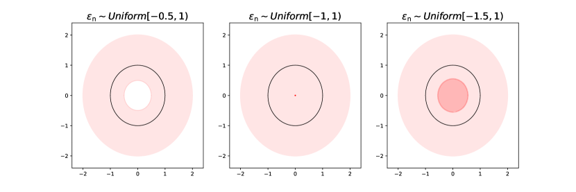
Figure 2: $Q$-normal reachability for different noise distributions $q_{\rm{n}}(\tilde{x}|x)$ used to inflate $\mathcal{X}=S^{1}$ (black line). Left: $\mathcal{X}$ is $Q$-normally reachable since every point in the inflated space $\widetilde{\mathcal{X}}$ (red shaded area) has a unique generator. Middle: $\mathcal{X}$ is Q-normally reachable since $\mathbb{P}_{\tilde{X}}-$almost every point in $\widetilde{\mathcal{X}}$ has a unique generator. Right: $\mathcal{X}$ is not Q-normally reachable since every point in the dark shaded area has two generators. Note that the pink area denotes the inflated manifold and not the density.

From a generative perspective, $Q-$normal reachability ensures that the mapping

$$\tilde{f}:\mathcal{U}\times\mathcal{V}\mapsto \widetilde{\mathcal{X}}$$

$$(u,v)\mapsto f(u)+A_{u}v$$ (8)

is bijective (up to a set of measure $0$). As $f$ is an embedding by assumption, $\tilde{f}$ is even a diffeomorphism if $||v||_{2}$ is sufficiently small, as we will show in theorem 4. This, together with the assumption that the prior is factorized, i.e. $\pi(u,v)=\pi_{u}(u)\pi_{v}(v)$, implies that the density $q_{\rm{n}}(\tilde{x})$ is given by

$$q_{\rm{n}}(\tilde{x})=\left|\det G_{\tilde{f}}(\tilde{x})\right|^{-\frac{1}{2}}\pi_{u}(u)\pi_{v}(v)$$ (9)

where $(u,v)=\tilde{f}^{-1}(\tilde{x})$. When setting $v=0$, we have that $\tilde{x}=x$ and indeed equation (7) holds as we will show that $\left|\det G_{\tilde{f}}(x)\right|=\left|\det G_{f}({x})\right|$ and $\pi_{v}(0)=q_{\rm{n}}(x|x)$. Note that our flow of arguments does not require the manifold $\mathcal{X}$ to be generated by a single chart $f$. Hence, as long as the manifold is $Q-$normal reachable, equation (9) holds locally for any chart $f$.

Theorem 4

Let $\mathcal{X}$ be a $d-$dimensional, $C^{2}$ manifold. For each $x\in\mathcal{X}$, let $q_{\rm{n}}(\cdot|x)$ denote a continuous distribution with support $N_{q(\cdot|x)}$ in the normal space of $x$, i.e. $N_{q(\cdot|x)}\subseteq N_{x}$, such that $x\in N_{q(\cdot|x)}$. Further, assume that the prior of the inflated random variable $\tilde{X}=X+\mathcal{E}_{\rm{n}}$ is factorized. If $\mathcal{X}$ is $Q-$normally reachable where $Q:=\{q_{\rm{n}}(\cdot|x)\}_{x\in\mathcal{X}}$, then for all $x\in{\mathcal{X}}$ it holds that $q_{\rm{n}}(x)=p^{*}(x)q_{\rm{n}}(x|x)$, thus

$$p^{*}(x)=\frac{q_{\rm{n}}(x)}{q_{\rm{n}}(x|x)}.$$ (10)

The proof can be found in Appendix A.1. As a consequence of theorem 4 , if the density $q_{\rm{n}}(\tilde{x})$ can be learned exactly using a single NF (which is e.g. the case whenever the inflated space $\tilde{\mathcal{X}}$ is diffeomorphic to $\mathbb{R}^{D}$ and the NF is sufficiently expressive), the true density $p^{*}(x)$ can be retrieved exactly.

Proposition 5

With the assumptions from theorem 4 , if the inflation is such that $\widetilde{\mathcal{X}}$ is diffeomorphic to $\mathbb{R}^{D}$, then $q_{\rm{n}}(\tilde{x})$ can be learned exactly using a single NF denoted as $F$, i.e. $q_{\rm{n}}(\tilde{x})=(\det G_{F}(F^{-1}(\tilde{x})))^{-\frac{1}{2}}\mathcal{N}(F^{-1}(\tilde{x});0,1)$. Then, using equation (10) the true density $p^{*}(x)$ can be calculated exactly.

Remark 6

It is important to note that the density $q_{\rm{n}}$ is with respect to the Euclidean metric because this ensures that we can learn it using an NF. If we consider the density with respect to the product metric on $\widetilde{\mathcal{X}}$ denoted as $q^{\otimes}_{\rm{n}}$, we can’t use a standard NF to learn it. However, we prove in the Appendix A.3 that with the assumptions of theorem 4 , we have that $q^{\otimes}_{\rm{n}}(\tilde{x})=p^{*}(x)q_{\rm{n}}(\tilde{x}|x)$ which is based on the fact that $\widetilde{\mathcal{X}}$ isomorphic to $\bigcup_{x\in\mathcal{X}}\left(\{x\}\times N_{q_{\rm{n}}(\cdot|x)}\right)$ up to set of measure $0$.

3.3 Gaussian noise as normal noise and the choice of $\sigma^{2}$

Our proposed method depends on three critical points. First, we need to be able to sample in the normal space of $\mathcal{X}$. Second, we need to determine the magnitude and type of noise. Third, we need to make sure that the conditions of theorem 4 are fulfilled. We address (partially) those three points.  
 
1. We show that for an increasing embedding dimension $D$, a full Gaussian noise is an increasingly good approximation for a Gaussian noise restricted to the normal space if we keep $d$ fixed. For that, consider $\mathcal{E}=\mathcal{E}_{\rm{t}}+\mathcal{E}_{\rm{n}}$, $\mathcal{E}\sim\mathcal{N}(0,\sigma^{2}I_{D})$. Then, the expected absolute squared error when approximating normal noise with full Gaussian noise is $\mathbb{E}\left[||\mathcal{E}-\mathcal{E}_{\rm{n}}||_{2}^{2}\right]=\mathbb{E}\left[||\mathcal{E}_{\rm{t}}||_{2}^{2}\right]=d\sigma^{2}.$ The expected relative squared error is therefore

$$\mathbb{E}\left[\frac{||\mathcal{E}-\mathcal{E}_{\rm{n}}||_{2}^{2}}{||\mathcal{E}_{\rm{n}}||_{2}^{2}}\right]=\mathbb{E}\left[\frac{||\mathcal{E}_{\rm{t}}||_{2}^{2}}{||\mathcal{E}_{\rm{n}}||_{2}^{2}}\right]=d\mathbb{E}\left[\frac{\sigma^{2}}{||\mathcal{E}_{\rm{n}}||_{2}^{2}}\right]=\frac{d}{D-d-2}$$ (11)

because $\mathcal{E}_{\rm{t}}$ and $\mathcal{E}_{\rm{n}}$ are independent and $\frac{\sigma^{2}}{||\mathcal{E}_{\rm{n}}||_{2}^{2}}$ follows a inverse $\chi^{2}-$distribution with $D-d$ degrees of freedom and therefore its expectation is $1/(D-d-2)$. Thus, for increasing $D$ while keeping $d$ fixed, Gaussian noise will be increasingly a better approximation for a Gaussian in the normal space. We denote the inflated density with Gaussian noise by $q_{\sigma}(\tilde{x})$ in the following.  
 
2. The inflation must not garble the manifold too much. For instance, adding Gaussian noise with magnitude $\sigma\geq r$ to $S^{1}$ will blur the circle. Since the curvature of the circle is $1/r$, intuitively, we want $\sigma$ to scale with the second derivative of the generating function $f$. Additionally, we do not want to lose the information of $p^{*}(x)$ by inflating the manifold. If the generating distribution $\pi(z)$ makes a sharp transition at $z_{0}$, $\pi(z_{0}-\Delta z_{o})\ll\pi(z_{0}+\Delta z_{o})$ for $|\Delta z_{o}|\ll 1$, adding to much noise in $x_{0}=f(z_{0})$ will smooth out that transition. Hence, we want $\sigma$ to inversely scale with $\pi^{\prime\prime}(z)$. We formalize these intuitions in proposition 7 and prove it in Appendix A.4. In accordance with theorem 4, we say that $p_{\sigma}(\tilde{x})$ approximates well $p^{*}(x)$ if $\lim_{\sigma\to 0}p_{\sigma}(x)/q_{\rm{n}}(x|x)=p^{*}(x)$ for all $x\in\mathcal{X}$ where $q_{\rm{n}}(x|x)$ is the normalization constant of a $(D-d)-$dimensional Gaussian distribution.

Proposition 7

Let $X\in\mathbb{R}^{D}$ be generated by $U\sim\pi_{u}(u)$ through an embedding $f:\mathbb{R}^{d}\to\mathbb{R}^{D}$, i.e. $f(U)=X$. Let $\pi_{u}\in C^{2}(\mathbb{R}^{d})$. For $q_{\sigma}(\tilde{x})$ to approximate well $p^{*}(x)$, in the sense that $\lim_{\sigma\to 0}q_{\sigma}(x)/q_{\rm{n}}(x|x)=p^{*}(x)$ for $x\in\mathcal{X}$, a necessary condition is that:

$$\sigma^{2}\ll\frac{2\pi_{u}(u_{0})}{||\pi_{u}^{\prime\prime}(u_{0})\odot(J_{f}^{T}(u_{0})J_{f}(u_{0}))^{-1}||_{+}}$$ (12)

where $||A||_{+}=\left|\sum_{i,j=1}^{d}A_{ij}\right|$ for $A\in\mathbb{R}^{d\times d}$, and $\odot$ denotes the elementwise product, and $(\pi^{\prime\prime}(u_{0}))_{ij}=\frac{\partial^{2}\pi_{u}(u)}{\partial u_{i}\partial u_{j}}|_{u=u_{0}}$ is the Hessian of $\pi_{u}$ evaluated at $u_{0}=f^{-1}(x)$.

Intuitively, a second necessary condition is that the noise magnitude should be much smaller than the radius of the curvature of the manifold which directly depends on the second-order derivatives of $f$. This can be illustrated in the following example:

Example 3

For the circle in $\mathbb{R}^{2}$ generated by $f(u)=(\cos(u),\sin(u))^{T}$ and a von Mises distribution $\pi_{u}(u)\propto\exp(\kappa\cos(u))$, we get that $\sigma^{2}\ll\min\left(\left|\frac{2r^{2}}{\kappa(\kappa\sin^{2}(u)-\cos(u))}\right|,r^{2}\right)$ where the first condition comes from proposition 7 and the second one comes from the curvature argument.

Even though this bound may not be useful as such in practice when $f$ and $\pi_{u}$ are unknown, it can still be used if $f$ and $\pi_{u}$ are estimated locally with nearest neighbor statistics.

From a numerical perspective, inflating a manifold using Gaussian noise circumvents degeneracy problems when training a vanilla NF for low-dimensional manifolds. In particular, the flows Jacobian determinant becomes numerically unstable, see equation (3). This determinant is essentially a volume-changing factor for balls. From a sampling perspective, these volumes can be estimated with the number of samples falling into the ball divided by the total number of points. Therefore, we suggest to lower bound $\sigma$ with the average nearest neighbor obtained from the training set to make sure that these volumes are not empty and thus avoid numerical instabilities.

3. Intuitively, if the curvature of the manifold is not too high and if the manifold is not too entangled, $Q-$normal reachability is satisfied for a sufficiently small magnitude of noise. In the manifold learning literature, the entanglement can be measured by the reach number. Informally, the reach number provides a necessary condition on the manifold such that it is learnable through samples, see Chapter 2.3 in Berenfeld and Hoffmann (2019).

Formally, the reach number is the maximum distance $\tau_{\mathcal{X}}$ such that for all $\tilde{x}$ in a $\tau_{\mathcal{X}}-$neighborhood of $\mathcal{X}$, the projection onto $\mathcal{X}$ is unique. In Appendix A.5 we prove theorem 8 which states that any closed manifold $\mathcal{X}$ with $\tau_{\mathcal{X}}>0$ is $Q-$normally reachable.

Theorem 8

Let $\mathcal{X}\subset\mathbb{R}^{D}$ be a closed $d$-dimensional manifold. If $\mathcal{X}$ has a positive reach number $\tau_{\mathcal{X}}$, then $\mathcal{X}$ is $Q-$normally reachable where $Q:=\{q_{\rm{n}}(\cdot|x)\}_{x\in\mathcal{X}}$ is the collection of uniform distributions on a ball with radius $\tau_{\mathcal{X}}$, i.e. $q_{\rm{n}}(\tilde{x}|x)=\mathrm{Uniform}(B(x,\tau_{\mathcal{X}})\cap N_{x})$ where $B(x,\tau_{\mathcal{X}})=\{y\in\mathbb{R}^{D},\text{s.t. }||x-y||_{2}<\tau_{\mathcal{X}}\}$ denotes the $D-$dimensional ball with radius $\tau_{\mathcal{X}}$ and center $x$.

To appreciate theorem 8, we refer to the Tubular Neighborhood theorem, which states that every smooth and compact manifold has positive reach (see e.g. Lee (2019) for a proof).

4 Related work

Here, we give an overview of methods based on NFs for density estimation on low-dimensional manifolds. One direction of research concentrates on densities defined on a given manifold, such as spheres, tori or hyperboloids (Rezende and Mohamed, 2015,Rezende et al., 2020, Mathieu and Nickel, 2020, Lou et al., 2020). Orthogonal to that direction, Brehmer and Cranmer, 2020, Beitler et al., 2018, Kim et al., 2020, Cunningham et al., 2020 do not rely on an explicit chart while focusing on improving the generative ability. From the latter works, only Brehmer and Cranmer (2020) learn, in theory, the density on the manifold $p^{*}(x)$ exactly.

Cunningham et al., 2020 assume that data live on a noisy, i.e. inflated manifold and propose to learn a stochastic inverse $q(z|\tilde{x})$ of the generator $q(\tilde{x}|z)$. To train the parameters of $q(\tilde{x}|z)$, they rely on variational inference making this approach a special case of a Variational Auto Encoder. Their injective noisy flow improves the sampling quality compared to a baseline NF and, in addition, learns a latent representation. However, by construction, they only learn the inflated distribution $q(\tilde{x})$.

Kim et al., 2020 follow our methodology closely by inflating the manifold so that a usual NF can be used to learn the inflated density. For each sample $x$, they first draw a value $c$ uniformly on $[0,0.1]$, and then add a sample $\nu$ from $\mathcal{N}(0,c^{2}I_{D})$ to $x$, i.e. $\tilde{x}=x+\nu$. They learn the conditional distribution of the inflated manifold, $q(\tilde{x}|c)$, allowing for sampling on the manifold by setting $c=0$. Their method does not require any knowledge of the manifold (neither the chart, nor the dimensionality), and improve 3D point cloud generation. However, they don’t provide a deflation of the inflated distribution, and thus don’t learn $p^{*}(x)$ exactly.

Beitler et al., 2018 propose to use different reference measures for the flow to encode the relevant manifold and irrelevant off-manifold directions. They propose to model the first $d$ latent variables, say $u$, of the flow as standard Gaussian and the remaining $D-d$ variables, say $v$, as a diagonal Gaussian with small variance. The hope is that maximum likelihood training is sufficient to encode the manifold in the first $d$ components, so that a sampling procedure where the remaining $D-d$ components are set to 0, i.e. $v=0$, would produce samples on the manifold. The gist is very similar to our idea expressed in equation (7). However, in general, this does not lead to the right density on the manifold, as explained in a footnote on page 4 in Brehmer and Cranmer, 2020, which justifies the name Pseudo-invertible encoder (PIE). Nevertheless, as noted by Brehmer and Cranmer, 2020, it is surprising that ”somehow in practice learning dynamics and the inductive bias of the model seem to couple in a way that favor an alignment of the level set $v=0$ with the data manifold. Understanding these dynamics better would be an interesting research goal.” Our work gives a theoretical explanation of why the PIE-model favors that alignment: When adding noise with small magnitude to the dataset (e.g. dequantization for images), the resulting density can be well approximated by a product of $p^{*}(x)$ and the noise distribution $q(\tilde{x}|x)$, such that treating the latent variables $u$ and $v$ differently, and thus having a product of two different measures as reference measure, biases the flow to learn this product form. A further interesting future direction would be to make this bias more explicit by constructing a flow for which the Jacobian determinant is in such a product form as well.

In Brehmer and Cranmer, 2020, the generating chart $f:\mathbb{R}^{d}\to\mathbb{R}^{D}$ is learned simultaneously with $p^{*}(x)$. They first transform $x$ using a usual flow on $\mathbb{R}^{D}$, and then project to the first $d$ components which is their proposal for $f^{-1}$. They then use another flow to learn the latent density $\pi_{u}$. To avoid calculating the Gram determinant of $f$, which is computationally expensive especially for $D\gg d$, they propose to train the parameters of $f$ using the mean squared error while updating the parameters of $\pi_{u}$ using maximum likelihood. They call the former manifold learning phase and the latter density learning phase. Different learning schemes (alternating and sequential) are proposed to ensure that $f$ encodes the manifold and $\pi$ captures the density. For the alternating scheme, they alternate for every epoch between a manifold training phase (updating the parameters of $f$), and the density training phase (updating the parameters for learning $\pi_{u}$). The experiments conducted by Brehmer and Cranmer, 2020 seem to verify that, indeed, $p^{*}(x)$ is learned exactly. Nevertheless, the ad-hoc training procedures without a unified maximum likelihood objective requires some further experimental verification.

State-of-the-art methods for image generation based on NF dequantizes the training data as a preprocessing step, see e.g. Kingma and Dhariwal, 2018. This dequantization is essentially an inflation of the data-manifold and is typically based on uniform noise. For images, it is generally assumed that $D\gg d$, and thus a dequantization based on Gaussian noise allows us to interpret the dequantization as a thickening of the data-manifold in the normal direction.

5 Results

We have three goals in this section: first, we numerically confirm the scaling factor in equation (10) for different manifolds. Second, we verify that Gaussian noise can be used to approximate a Gaussian noise restricted to the normal space. Third, we numerically test the bounds for $\sigma^{2}$ derived in Section 3.3. For training details, we refer to Appendix B.2. The code for our experiments can be found on https://github.com/chrvt/Inflation-Deflation.

The standard procedure for our experiments and for evaluating the learned density is the following:

1. Data generation: We sample latent variables $u\sim\pi_{u}(u)$ for a given $\pi_{u}(u)$, and generate points $x$ on the manifold using a mapping $f$, i.e. $x=f(u)$.

2. Inflation: We add noise $\varepsilon$ to $x$, $\tilde{x}=x+\varepsilon$, either in the normal space $N_{x}$ or in the full ambient space. As an acronym for our inflation-deflation method we use ID. In particular, when the inflation is performed in the normal space, we call the method Normal Inflation Deflation (NID) and when the inflation is isotropic, we call it Isotropic Inflation Deflation (IID).

3. Training: We learn the inflated distribution, i.e. $q_{\sigma}(\tilde{x})$ in case of isotropic noise or $q_{\rm{n}}(\tilde{x})$ in case of normal noise, using a Block Neural Autoregressive Flow (BNAF) introduced in De Cao et al. (2020).

4. Deflation: Given an estimator $\hat{q}_{\rm{n}}(\tilde{x})$, we use equation (10) to calculate $p^{*}(x)$. For a $d-$dimensional manifold embedded in $\mathbb{R}^{D}$, the scaling factor when using Gaussian noise is $q_{\rm{n}}(x|x)=(2\pi\sigma^{2})^{\frac{d-D}{2}}$.

5. Quantitative evaluation: To quantify the quality of the learned density beyond visual similarity, we use the estimate of $p^{*}(x)$ to approximate $\pi_{u}(u)$. These densities are related through the Gram determinant of the generating mapping $f$, $\det G_{f}$, see Section 2 . For that, we calculate the KS statistics between this estimate $\hat{\pi}$ and the ground truth $\pi$. The KS statistic is defined as

   $$KS=\sup_{u\in\mathcal{U}}|F(u)-G(u)|$$ (13)

   where $F$ and $G$ are the cumulative distribution functions associated with the probability densities $\pi_{u}(u)$ and $\hat{\pi}_{u}(u)$, respectively. By definition, $KS\in[0,1]$ and $KS=0$ if and only if $\pi_{u}(u)$ is equal to $\hat{\pi}_{u}(u)$ for almost every $u\in\mathcal{U}$. Note that, if our estimate does not yield a density on the manifold (i.e. it is not normalized to $1$), the KS statistics still serves as a relative performance measure as the KS value will be lower bounded by a strictly positive number in this case ($1$ minus the corresponding normalization constant).
   In 2D, comparing two random variables based on $\mathbb{P}(X_{1}\leq x_{1},X_{2}\leq x_{2})$ or based on $\mathbb{P}(X_{1}\leq x_{1},X_{2}\geq x_{2})$ (or any of the other two combinations) may lead to different results. Hence, for the KS value in 2D, we need to calculate the KS statistics based on all possible orderings and then take the maximum.

6. $\sigma^{2}-$bounds: In proposition 7, we derived a necessary condition in form of an upper bound $\sigma_{\text{Prop}}^{2}$ for $\sigma^{2}$ such that NID can be well approximated by IID. In addtion, we argued that $\sigma^{2}$ should not exceed the curvature radius, see example 3. For $d=1$, this curvature radius is straight forward computed using the first and second derivatives of the generating mapping. For $d=2$, we use the Gauss curvature $\sigma_{\text{Gauss}}^{2}$ instead, see e.g. Do Carmo (2016). Therefore, as upper bound for $\sigma^{2}$, we sample $10^{4}$ points from the target distribution, calculate $\min\{\sigma_{\text{Prop}}^{2},\sigma_{\text{Gauss}}^{2}\}$ for each point, and then take the average. For manifolds with $\sigma_{\text{Gauss}}^{2}=0$, we only use $\sigma_{\text{Prop}}^{2}$. As a lower bound $\sigma_{\text{LB}}^{2}$, we proposed to calculate the $L_{2}-$distance to the nearest neighbour. Therefore, we sample $10^{4}$ points from the target distribution, calculate the nearest neighbour for each point, and then take the average

7. Benchmarking: For a known manifold consisting of a single chart $f$, Gemici et al. (2016) used $f$ to encode the manifold into the corresponding latent space $\mathbb{R}^{d}$, and then learn the latent density using a standard NF. However, manifolds such as spheres or tori, cannot be described using a single chart. In Brehmer and Cranmer (2020), such degeneracy problems were avoided numerically by simply moving points that are close to singularities away from them. As a consequence, the density close to these singularities cannot be learned exactly (we illustrate this in the first experiment on $\mathbb{S}^{1}$). In Brehmer and Cranmer (2020), this method is named Flow on manifolds (FOM) and we stick to this notation in the following. In our case, as we are evaluating the qualitive performance using the KS-statistics on the latent densities, we simply train a standard NF directly on the latent space for the remaining experiments (thus avoiding potential degeneracy problems altogether).

Remark 9

For our qualitative evaluation using the KS-statistics, we rely on being able to relate the density in the data-space $p^{*}(x)$ with the latent distribution $\pi_{u}(u)$ via the Gram determinant of the manifold generating mapping $f$. If $f$ consists of singularities, the KS-statistics is still well-defined if these singularities have $0$ measure (as it is the case for e.g. spheres or tori). However, note that our method does not rely on a specific embedding and thus avoids degeneracy problems during training. The IID model does not even need any explicit knowledge of the manifold except its dimensionality for the right scaling factor. We validate the generality of our method by learning a manifold which cannot be described by a single chart covering all the points up to a set of measure $0$. For that, we glue a half sphere with the positive part of a hyperboloid (compactly denoted as $(\mathbb{HS})^{2}$), see table 2 .

5.1 Proof of concept: $\mathbb{S}^{1}$

We start with a circle of radius $3$, a $1-$dimensional manifold embedded in $\mathbb{R}^{2}$, see table 1 .

feature	$\mathcal{U}$	$f(u)$	$\det G_{f}(x)$
closed	$[-\frac{\pi}{2},\frac{\pi}{2}]$	$3\begin{pmatrix}\cos(u)\\ \sin(u)\end{pmatrix}$	$3$

Table 1: Characteristics of $\mathbb{S}^{1}$.

We let $\pi_{u}(u)\propto\exp(8\cos(u))$ be a von Mises distribution.
 
Inflation and Deflation: We inflate $\mathcal{X}$ using 3 types of noise: Gaussian in the normal space (NID), Gaussian in the full ambient space (IID), and $\chi_{2}$-noise in the normal space as described in example 1(b) with scale parameter $3$. Technically, Gaussian noise violates the $Q-$normal reachability assumption. However, if $\sigma^{2}$ is small and the scale parameter for the von Mises distribution is large enough, this is practically fulfilled. Given an estimator for $q_{\rm{n}}(\tilde{x})$, we use equation (10) to calculate $p^{*}(x)$. For the IID and NID methods, we have that $q_{\rm{n}}(x|x)=1/\sqrt{2\pi\sigma^{2}}$ and for the normal $\chi^{2}-$noise is $q_{\rm{n}}(x|x)=\sqrt{3}e^{-3/2}/(\sqrt{8}\Gamma(\frac{3}{2}))$.

5.1.1 Full Gaussian vs. Normal space noise

In Figure 3, we show the results for $\sigma^{2}=0.01$ and $\sigma^{2}=1$. In the respective plot, the first row shows training samples from the inflated distributions $q_{\sigma}(\tilde{x})$ (left), and $q_{\rm{n}}(\tilde{x})$ (middle), respectively. We color code a sample $\tilde{x}=x+\varepsilon$ according to $p^{*}(x)$ to illustrate the impact of noise on the inflated density. Note that the FOM model (top right) does not need any inflation and therefore is trained on samples from $p^{*}(x)$ only. In the respective plot, the second row shows the learned density for the different models and compares it to the ground truth von Mises distribution $\pi_{u}(u)$ depicted in black. As we can see, for $\sigma^{2}=0.01$ all models perform very well, although the FOM model slightly fails to capture $p(u)$ for $u$ close to $0$ which corresponds to the chosen singularity point (see point 5. in the standard procedure description). For $\sigma^{2}=1$, we see a significant drop in the performance of the Gaussian model. Although the manifold is significantly disturbed, the normal noise model still learns the density almost perfectly , so does the normal $\chi^{2}-$noise model, as predicted by theorem 4.

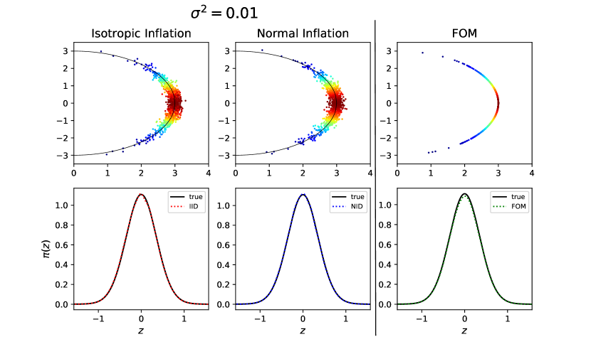
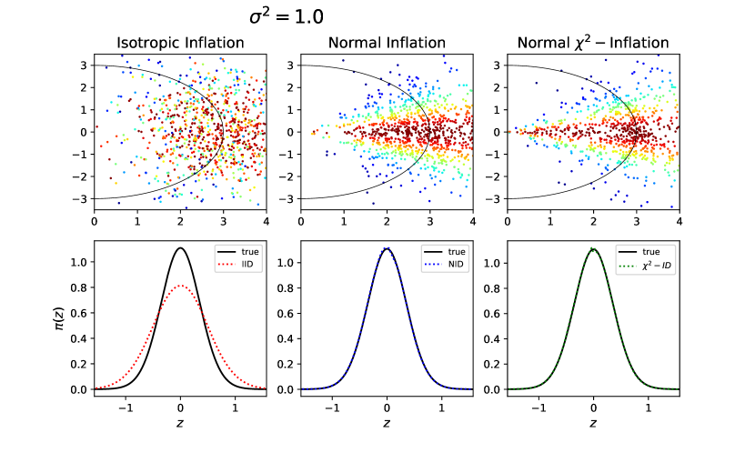
Figure 3: Learned densities for $\sigma^{2}=0.01$ (above) and $\sigma^{2}=1$ (below), respectively. First row: Samples used for training the respective model: IID (left), NID (middle), FOM/ $\chi^{2}$ (right). The black line depicts the manifold $\mathcal{X}$ (a circle with radius 3) and the colors code the value of $p^{*}(x)$. Second row: Colored line: Learned density $\hat{\pi}_{u}(u)$ according to equation (10) multiplied by 3. Blackline: ground truth von Mises distribution.

5.1.2 Noise dependence and higher embedding dimensions

To measure the dependence of our method on the magnitude of noise, we iterate this experiment for various values of $\sigma^{2}$ and estimate the Kolmogorov-Smirnov (KS) statistics. In Figure 4, we display the KS values depending on different levels of noise, for the NID (blue) and IID (orange) methods compared with the ground truth von Mises distribution. Also, we embed the circle into higher dimensions $D=5,10,15,20$ and repeat this experiment. The result for $D=2$ and $D=20$ are shown in the first row (left and right). We add the performance of the FOM model (which is independent of $\sigma^{2}$) horizontally. Besides, we depict the lower and upper bound for $\sigma^{2}$ from section 3.3 with dashed vertical lines. In the lower-left image, we show the optimal $KS$ values obtained for both models depending on $D$. The lower-right image shows the corresponding $\sigma^{2}$ for those optimal $KS$. In bright, the optimal average $\sigma^{2}$ is shown whereas the dark regions are the minimum respectively maximum values for $\sigma^{2}$ such that we outperformed the FOM benchmark. We note that for both cases, the averaged optimal $\sigma^{2}$ is within the predicted bounds for $\sigma^{2}$ (depicted as dashed black horizontal lines).

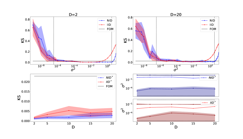
Figure 4: KS values for the NG- (blue) and IID-noise method (orange) depending on $\sigma^{2}\in[10^{-9},10]$ and the embedding dimension $D=5,10,15,20$ in log-scale. For $D=2$ (top left) and $D=20$ (top right), the two vertical lines represent the lower and upper bound for $\sigma^{2}$ estimated according to Chapter LABEL:sec:IID_as_NS with 10K samples. We plot horizontally the KS value obtained from FOM. Bottom left: Optimal KS values depending on $D$. Bottom right: Optimal averaged $\sigma^{2}$ such that optimal $KS$ is obtained (bright). The maximum and minimum $\sigma^{2}$ such that the FOM benchmark is outperformed (dark). The dashed horizontal lines are again the theoretical bounds. We used 10 seeds for the error bars and plot in log-scale.

The optimal KS values do not change much depending on $D$, and the NID and IID models approach each other, as predicted.

Interestingly, the onset for the increase in the KS value for the NID noise is roughly 3 which is the radius of the circle. For increasing $\sigma^{2}$, $\tilde{\mathcal{X}}$ resembles more and more a double cone which is not diffeomorphic to $\mathbb{R}^{2}$ and thus the NF used to train the inflated distribution may not be able to capture the density close to the circle’s center correctly. Also, the $Q-$normal reachability is more and more violated with an increasing $\sigma^{2}$.

5.2 Densities on surfaces

We show that we can learn different distributions on different manifolds, see table 2 for an overview of those manifolds and their characteristics.

Manifold	feature	$\mathbf{\mathcal{U}}$	$\mathbf{f(u)}$	$\mathbf{\det G_{f}(x)}$
$\mathbb{S}^{2}$	closed	$[0,2\pi]\times[0,\pi]$	$\begin{pmatrix}\cos(z_{1})\sin(z_{2})\\ \sin(z_{1})\sin(z_{2})\\ \cos(z_{2})\end{pmatrix}$	$\sin(z_{2})$
$\mathbb{T}^{2}$	closed	$[0,2\pi]\times[0,2\pi]$	$\begin{pmatrix}(1+0.6\cos(z_{2}))\cos(z_{1})\\ (1+0.6\cos(z_{2}))\sin(z_{1})\\ 0.6\sin(z_{2})\end{pmatrix}$	$0.6(1+0.6\cos(z_{2}))$
$\mathbb{H}^{2}$	diffeom. to $\mathbb{R}^{2}$	$[0,+\infty)\times[0,2\pi]$	$\begin{pmatrix}\sinh(z_{1})\cos(z_{2})\\ \sinh(z_{1})\sin(z_{2})\\ \cosh(z_{1})\end{pmatrix}$	$(\sinh^{2}(z_{1})+\cosh^{2}(z_{1}))\sinh^{2}(z_{1})$
thin spiral	open	$(0,+\infty)$	$3\pi\sqrt{z}\begin{pmatrix}-\cos(3\pi\sqrt{z})\\ \sin(3\pi\sqrt{z})\end{pmatrix}$	$\frac{1+(3\pi\sqrt{z})^{2}}{(3\pi\sqrt{z})^{2}}$
swiss roll	open	$(0,1)\times(0,1)$	$\begin{pmatrix}(\alpha+3\pi z_{2})\cos(\alpha+3\pi z_{2})\\ 21z_{1}\\ (\alpha+3\pi z_{2})\sin(\alpha+3\pi z_{2})\end{pmatrix}$	$(63\pi)^{2}(1+(0.5+2z_{2})^{2})$
$(\mathbb{HS})^{2}$	chart 1	$(-\infty,0]\times[0,2\pi)$	$\begin{pmatrix}-\cosh(|z_{1}|)\cos(z_{2})\\ -\cosh(|z_{1}|)\sin(z_{2})\\ \sinh(|z_{1}|)\end{pmatrix}$	$(\sinh^{2}(|z_{1}|)+\cosh^{2}(|z_{1}|))\cosh^{2}(|z_{1}|)$
	chart 2	$[0,\frac{\pi}{2}]\times[0,2\pi)$	$\begin{pmatrix}\cos(z_{2})\cos(z_{1}+\pi)\\ \sin(z_{2})\cos(z_{1}+\pi)\\ \sin(z_{1}+\pi)\end{pmatrix}$	$\cos(z_{1}+\pi)$

Table 2: Characteristics of various manifolds.

In Figure 5, we show different target densities in data and latent space (columns A and B), along with the learned latent distributions using our method (as described in point 4. of the standard procedure) with the normal inflation-deflation method NID (column C). We take the model with $\sigma^{2}$ corresponding to the best KS value. In the last column D, we show how the KS-statistics depends on $\sigma^{2}$ using IID, NID, and the FOM baseline. We refer to Appendix B.2, B.2.1 and B.3.1 for the training details, exact latent densities and additional figures showing the learned latent densities using IID and FOM.

Remarkable, our method performs well on a wide range of manifolds and different target distributions. Whether the manifold is closed (A 1-2, 3-4), open (A 5-6, 7-9), or consists of multiple charts (A 10-11), whether the latent variables are idependent (B 1,3,6,8,10) or dependent (B 2,4,5,9,11), whether the distribution is supported on points for which the Gram determinant is $0$ (A 1-2) or on points for which the Gram determinant is arbitrarily large (A 7), the induced latent density (and therefore the data-density $p^{*}(x)$) is approximated well. This is not only reflected in the visual similarity to the target distribution (columns B vs. C), but also in the KS statistics (column D). Surprisingly, the best KS values for the IID and NID methods are of the same order as the FOM baseline (tables in D). This is striking as the IID and NID methods are trained in data space, in contrast to the FOM which is trained in latent space directly (see point 4. in the standard procedure). In some cases, the NID even outperforms the FOM significantly (see tables in D 2-3). The optimal KS value for IID is only slightly worse than the one for NID showing that indeed our method can even be used without any explicit knowledge of the manifold (except its dimensionality for the right scaling factor).
Note that the NID method always allows for a greater range of $\sigma^{2}$ compared to IID, except for the thin spiral for which both curves have almost the same course (D 7). As an extreme case, the geometry of the hyperboloid $\mathbb{H}^{2}$ even allows for very large values of $\sigma^{2}$ when using NID (D 5-6). Notably, almost all the KS curves are U-shaped. However, for the torus (D 3-4) and swiss roll (D 8-9) the KS value for IID decreases approaching $\sigma^{2}=10^{1}$ before increasing again. For increasing $\sigma^{2}$, the induced latent distribution $\hat{\pi}_{u}$ is increasingly flat. Then, certain values of $\sigma^{2}$ lead to the right scaling such that $\int_{\mathcal{U}}\hat{\pi}_{u}(u)du\approx 1$ which decreases the KS value.

Except for the Hyperboloid and thin spiral, D 6 and D 7, respectively, does the lower bound based on nearest neighbor statistics nicely predicts the magnitude of noise required to approximate $p^{*}(x)$ well using IID. Also the upper bound (which is $>10$ for the Swiss Roll in both cases, see D 8-9, and thus not seen in those figures) behaves as predicted. It is necessary (though not sufficient, see D 5-6) for $\sigma^{2}$ to be lower than this upper bound such that IID approximates NID well and thus can be used to approximate $p^{*}(x)$.

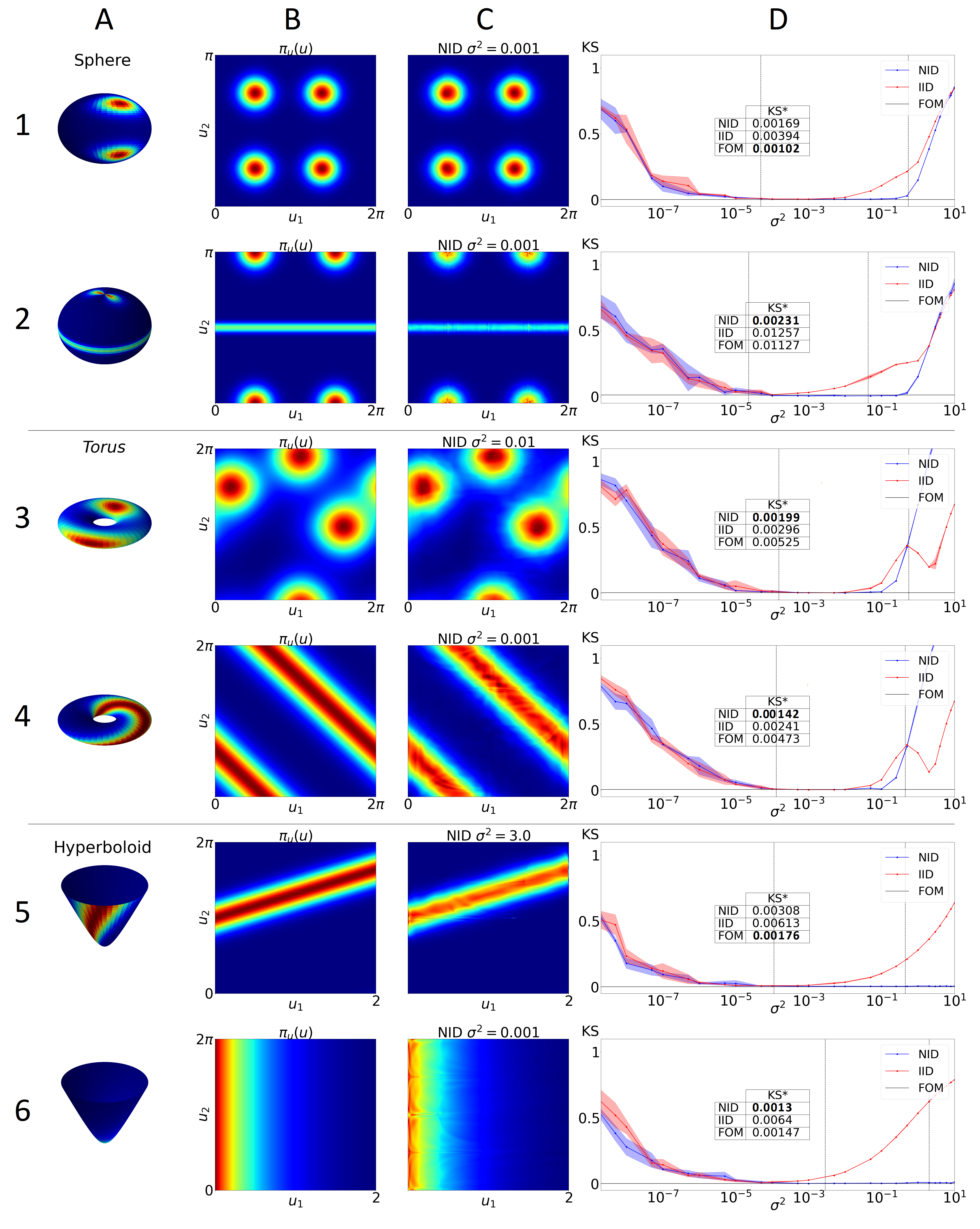
Figure 5: Columns A and B: Target density in data (A) and latent space (B) for various manifolds and different latent distributions. Column C: Best learned density using our method with the method NID. Column D: KS vs. $\sigma^{2}$ plot for the IID and NID methods (we used 3 seeds for the error bars) with the KS value of FOM as horizontal line. Table in D: Optimal KS values for the different models (best, i.e. lowest, in bold). Vertical Lines in C Lower and upper bound (see point 5. of the standard procedure).

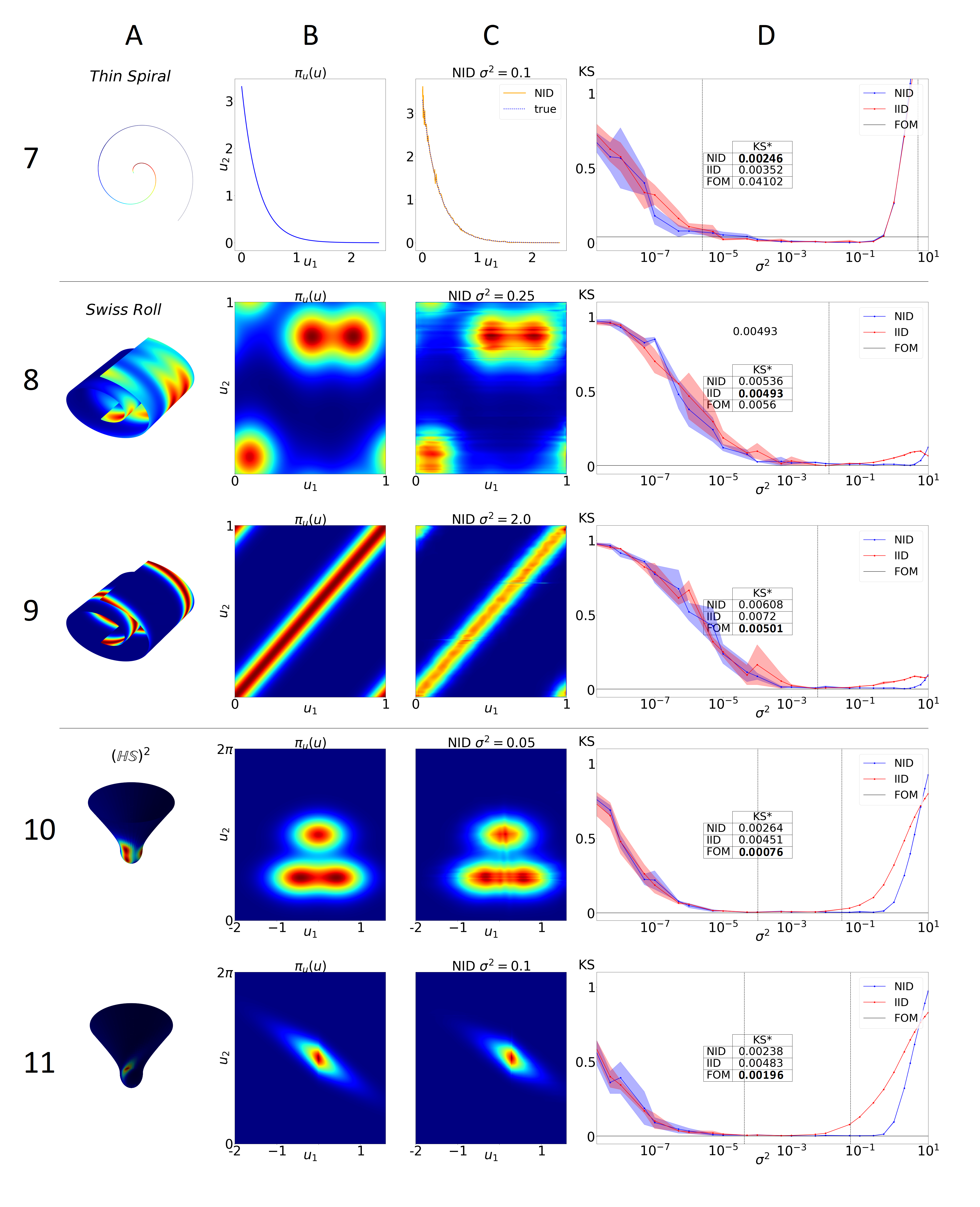
Figure 6: Figure 5 (continuation): Columns A and B: Target density in data (A) and latent space (B) for various manifolds and different latent distributions. Column C: Best learned density using our method with the method NID. Column D: KS vs. $\sigma^{2}$ plot for the IID and NID methods (we used 3 seeds for the error bars) with the KS value of FOM as horizontal line. Table in D: Optimal KS values for the different models (best, i.e. lowest, in bold). Vertical Lines in C Lower and upper bound (see point 5. of the standard procedure).

5.3 Density estimation on $SO(2)$

Finally, we consider the manifold consisting of orthonormal $k-$frames in $\mathbb{R}^{n}$,

$$\mathbb{S}^{n,k}:=\left\{V:=[v_{1},\dots,v_{k}]\in\mathbb{R}^{n\times k}\ s.t.\ V^{T}V=1\right\},$$ (14)

the Stiefel manifold. The dimension of this manifold is $nk-(k+1)k/2$. We consider the special case where $n=k=2$ in the following. Then, $\mathbb{S}^{2,2}$ is the orthogonal group $SO(2)$ with $\dim(\mathbb{S}^{2,2})=1$. We can represent an element in $SO(2)$ as $2$ orthogonal vectors on the unit circle embedded in $\mathbb{R}^{2}$. Therefore, as latent distribution $\pi_{u}$, we consider a mixture of 1-dimensional von Mises distributions $\pi_{u}$, and sample an element in $[x,x_{\bot}]\in SO(2)$ as follows:

1. we sample $u\sim\pi_{u}(u)$,

2. set $x=(\cos(u),\sin(u))^{T}$,

3. rotate $x$ and set $x_{\bot}=(-\sin(u),\cos(u))^{T}$.

Finally, we concatenate $x$ and $x_{\bot}$ to a single vector in $\mathbb{R}^{4}$ and learn the corresponding density using an NF, see Appendix B.2 and B.2.1 for the training details and exact latent densities, respectively.

In Figure 7, we plot the induced latent distributions (see point 4. of the standard procedure) using NID and IID (with the $\sigma^{2}$ corresponding to the best KS value) on top of the true latent distribution (Figures A and B). In Figure C, we show how the KS-statistics depends on $\sigma^{2}$ using IID, NID, and the FOM baseline.

Both, the NID and IID match the target distribution except at the peaks and some valleys of $\pi_{u}$. The estimate using IID is smoother, however, note that the KS-statistics does not account for the smoothness of the estimate. Indeed, an estimate using NID with e.g. $\sigma^{2}=0.01$ yields a similar smooth curve as the IID (see Figure 11 in Appendix B.3.1).
Surprisingly, the optimal KS value for IID is slightly better than the one for NID, both outperforming FOM (using a simple Gaussian-Kernel Density Estimate). However, NID always allows for a greater range of $\sigma^{2}$ compared to IID, as expected.

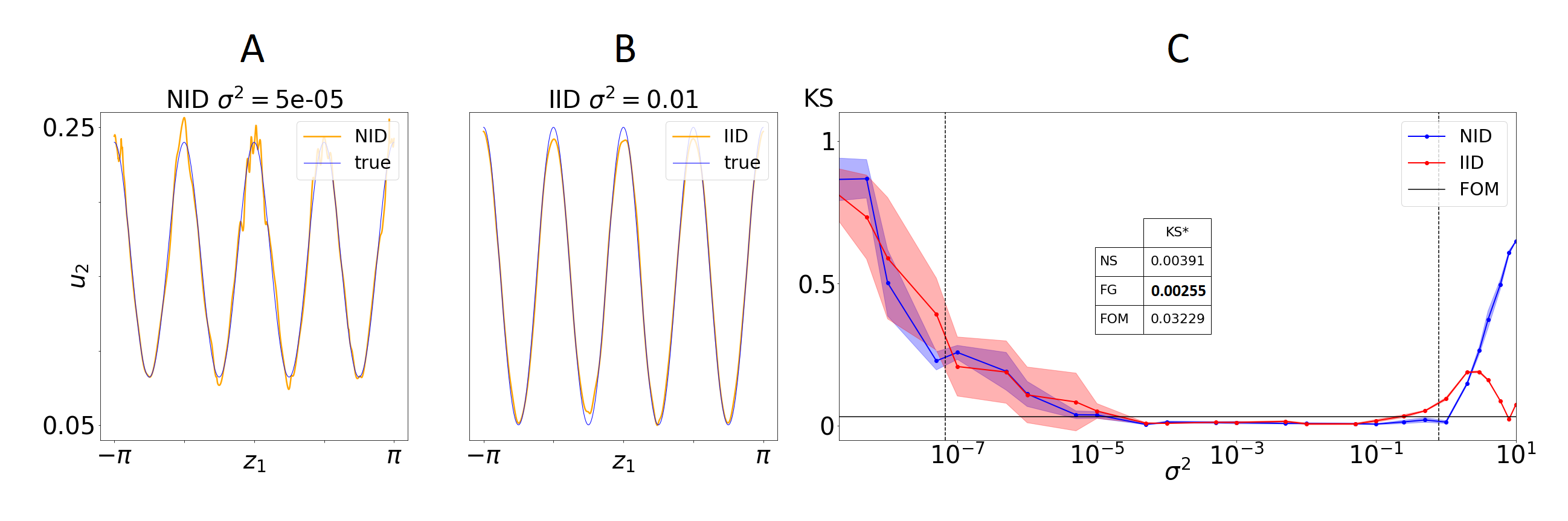
Figure 7: A: Learned latent density using NID (orange) on top of target latent density (blue). B: Learned latent density using IID (orange) on top of target latent density (blue). C: KS vs. $\sigma^{2}$ plot for IID and NID (we used 3 seeds for the error bars) with the KS value of FOM as horizontal line. Table in C: Optimal KS values for the different models (best, i.e. lowest, in bold). Vertical Lines in C: Lower and upper bound (see point 5. of the standard procedure).

5.4 Density estimation on MNIST

Finally, we end this section with an application on the handwritten digit dataset MNIST, Lecun et al. (1998). The manifold hypothesis states that real-world data, such as images, can be described by a few key features only, thus populating a low-dimensional manifold in the high-dimensional embedding space.

To estimate the density of e.g. digit 1 images, both the inflation-deflation method and the $\mathcal{M}-$flow need to know the manifold dimensionality $d$. Estimating this intrinsic dimensionality $d$ is an active research area, see e.g. Hein and Audibert (2005) and Facco et al. (2017). For instance, Hein and Audibert (2005) estimate the intrinsic dimensionality of MNIST digit 1 to be roughly $8$.

We test the utility of learned digit 1 likelihoods for out of distribution detection (OOD) using IID (isotropic inflation-deflation) and the $\mathcal{M}-$flow. In Figure 8, we show the log-likelihood densities (estimated using kernel density estimation) on the MNIST test set after training on digit 1 images from the training set only. For the IID, we preprocess the training set by adding Gaussian noise with $\sigma^{2}=0.1$ to the 8-bit images. For the $\mathcal{M}-$flow, we leave the training set unaltered. Though, we did not find this preprocessing (or the absence of it) to have a significant impact on the log-likelihoods for both methods. We refer to Appendix B.3 for more training details and additional plots for different preprocessing protocols.

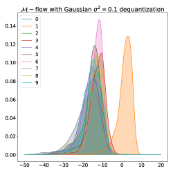
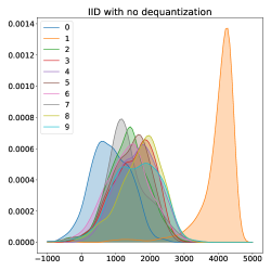
Figure 12: Log likelihoods on various MNIST test digits using $\mathcal{M}-$flow (left) and IID (right) trained on digit 1 only.

In Figure 8, we want to highlight two interesting observations. First, the log-likelihoods of digits other than $1$ are not significantly different using the IID or $\mathcal{M}-$flow method for OOD. One can see this by comparing the area of intersection of the digit $1$ density (orange) with the other digits (other colors). The greater this area, the more out of distribution examples (in this case MNIST digits other than 1) would be classified as digit $1$ when using a naive classifier based on an adhoc log-likelihood threshold. This area is $\approx 0.07$ for both methods. Our second observation is that the absolute log-likehood values differ substantially. As both method try to esitmate the density $p^{*}(x)$ supported on a low-dimensional manifold, we would have expected similar log-likelihood values. The fact that these values are several magnitudes apart, together with the observation that an inflation is not strictly necessary using an NF to learn the data-density (see Figure 12 in Section B.3.1), indicate that the MNIST digit 1 images do not strictly lie on a low-dimensional manifold embedded in $\mathbb{R}^{D},D=784$. In such a case, the $\mathcal{M}-$flow would still try to fit the training set onto a manifold which may lead to overfitting and unforeseeable log-likelihood values when evaluating on a test set. In contrast, the IID method is by construction robust to overfitting as the addition of isotropic noise leads to similar log-likelihood values in the vicinity of the data-manifold.

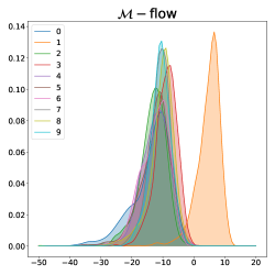
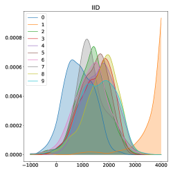
Figure 8: Log likelihoods on various MNIST test digits using $\mathcal{M}-$flow (left) and IID (right) trained on digit 1 only.

Finally, we want to revisit our remark on the computational complexity of the $\mathcal{M}-$flow, see Section 2 . To evaluate the density using the $\mathcal{M}-$flow, one needs to calculate the Gram determinant which has a computational complexity of $\mathcal{O}(d^{2}D)+\mathcal{O}(d^{3})$. Indeed, to evaluate 1000 digits using a batch size of 1, the $\mathcal{M}-$flow needs about $17.5$ hours. For the same amount, the inflation-deflation methods needs less than 10 seconds.

6 Discussion

To overcome the limitations of NFs to learn a density $p^{*}(x)$ defined on a low-dimensional manifold, we proposed to embed the manifold into the ambient space such that it becomes diffeomorphic to $\mathbb{R}^{D}$, learn this inflated density using an NF, and, finally, deflate the inflated density according to theorem 4. There, we provided sufficient conditions on the choice of inflation such that we can compute $p^{*}(x)$ exactly. Our method depends on some critical points which we addressed in Section 3.3. So far, the magnitude of noise $\sigma^{2}$ when using NFs on real-world data is somewhat chosen arbitrarily. As a step to overcome this arbitrariness, we derived an upper bound for $\sigma^{2}$ in proposition 7 and established an interesting connection to the manifold learning literature in theorem 8 . However, proposition 7 may not be very useful as such in real-world application and numerical methods need to be considered which potentially suffer from the curse of dimensionality. On a more positive note, our various experiments on different manifolds suggest that a great range for $\sigma^{2}$ lead to good results, even when using full Gaussian noise. Thus, including $\sigma^{2}$ into the standard hyperparameter search will likely suffice.
Our theoretical results open new research avenues. Using full Gaussian noise to learn the inflated distribution smears information on $p^{*}(x)$, in particular, if $p^{*}(x)$ has many local extrema. This loss of information may be especially impactful in out of distribution (OOD) detection or when it comes to adversarial robustness. Therefore, developing methods that allow generating noise in the manifold’s normal space could improve the performance of NFs on such tasks.
Another interesting direction is to exploit the product form of equation (7) and learn low-dimensional representations by forcing the NF to be noise insensitive in the first $d$-components and noise sensitive in the remaining ones. Inverting the corresponding flow allows sampling directly on the manifold.

Acknowledgments

We would like to thank Johann Brehmer for clarifying discussions on the manifold flow, and Simone C. Surace for useful discussions on manifolds.
This study has been supported by the Swiss National Science Foundation grant 31003A_175644.

A Appendix

A.1 Proof of theorem 4

Let $x\in\mathcal{X}$. Since $\mathcal{X}$ is a $d-$dimensional $C^{2}$ manifold, there exists an open neighborhood $\mathcal{B}_{x}$ of $x$ in $\mathcal{X}$, an open set $\mathcal{U}_{x}$ in $\mathbb{R}^{d}$, and an invertible map $f:\mathcal{U}_{x}\mapsto\mathcal{B}_{x}$, $\mathcal{U}_{x}\subset\mathbb{R}^{d}$, such that $f$ and $f^{-1}$ are twice continuously differentiable. It follows that the Gram determinant of $f$ is non-zero for all $x\in\mathcal{B}_{x}$, i.e. $\det G_{f}(x)\neq 0\ \forall x\in\mathcal{B}_{x}$. We exploit this by constructing a local diffeomorphism $\tilde{f}$ on the inflated space $\widetilde{\mathcal{X}}=\bigcup_{x\in\mathcal{X}}N_{q_{\rm{n}}(\cdot|x)}$ in the following.
For that, we denote by $A_{u}$ the matrix with columns consisting of normal vectors spanning the normal space in $x=f(u),u\in\mathcal{U}_{x}$. Without loss of generality we can set $\det A_{u}^{T}A_{u}=1$. With $\mathcal{V}_{x}\subset\mathbb{R}^{D-d}$, we define $\tilde{f}:\mathcal{U}_{x}\times\mathcal{V}_{x}\subset\mathbb{R}^{d}\times\mathbb{R}^{D-d}\to\widetilde{\mathcal{B}}_{x}$ for some $\widetilde{\mathcal{B}}_{x}\subset\widetilde{\mathcal{X}}$ as follows:

$$\tilde{f}(u,v)=f(u)+A_{u}v.$$ (15)

Note that, by assumption, $0\in\mathcal{V}_{x}$. Thus, for $v$ sufficiently small, i.e. $||v||<\varepsilon$ for some $\varepsilon>0$, $\tilde{f}$ is indeed a diffeomorphism which follows from the inverse function theorem. Our key observation is that

$$\det G_{\tilde{f}}(x)=\det G_{f}(x)$$ (16)

which allows us to relate the density on $\widetilde{\mathcal{X}}$ to the density on $\mathcal{X}$. For the sake of clarity, we prove equation (16) in Lemma 10 below.

Now let $\tilde{x}=x+\varepsilon_{\rm{n}}\in\widetilde{\mathcal{X}}$ such that $\tilde{x}\in\widetilde{\mathcal{B}}_{x}$. Since $\mathcal{X}$ is $Q-$normally reachable, $\mathcal{P}_{\tilde{X}}-$almost all $\tilde{x}$ are uniquely determined by some $(u,v)^{T}=\tilde{f}^{-1}(\tilde{x})\in\mathcal{U}_{x}\times\mathcal{V}_{x}$, and since $u$ and $v$ are sampled independently by assumption, it must hold that

$$q_{\rm{n}}(\tilde{x})=(\det G_{\tilde{f}}(\tilde{x}))^{-\frac{1}{2}}\pi_{u}(u)\pi_{v}(v)$$ (17)

where $\pi_{v}(v)$ is the noise generating latent distribution. Note that $q_{\rm{n}}(\tilde{x})$ is the density of $d\mathbb{P}_{\tilde{X}}$ with respect to the volume form $dV_{\tilde{f}}$. For $\tilde{x}=x$, we have that $v=0$ and thus

$$q_{\rm{n}}(x)=(\det G_{\tilde{f}}(x))^{-\frac{1}{2}}\pi_{u}(u)\pi_{v}(0).$$ (18)

Now since $\det G_{\tilde{f}}(x)=\det G_{{f}}(x)$, we have that

$$q_{\rm{n}}(x)= (\det G_{\tilde{f}}(x))^{-\frac{1}{2}}\pi_{u}(u)\pi_{v}(0)$$

$$= (\det G_{f}(x))^{-\frac{1}{2}}\pi_{u}(u)\pi_{v}(0)$$

$$= p^{*}(x)\pi_{v}(0)$$

$$= p^{*}(x)q_{\rm{n}}(x|x)$$ (19)

where in the last step we have used that the Gram determinant of the normal space generating mapping is $1$ such that $\pi_{v}(0)=q_{\rm{n}}(x|x)$. As $x$ was chosen arbitrarily on the manifold, this ends the proof.

Lemma 10

For $\tilde{f}$, $f$ and $x$ as defined above, we have that $\det G_{\tilde{f}}(x)=\det G_{{f}}(x)$.

Proof  The Jacobian of $\tilde{f}$ is given by

$$J_{\tilde{f}}(u,v)=\left[\begin{array}[]{c;{2pt/2pt}cc}J_{f}(u)+\frac{\partial}{\partial u}A_{u}v&\ A_u\end{array}\right]$$ (20)

where $\frac{\partial}{\partial u}$ denotes the Jacobian of a function depending on $u$, and the dashed line seperates two block matrices. Here we need that $f\in C^{2}$ to ensure the Jacobian is real. For points on the manifold is $v=0$, and thus the Gram determinant reduces to

$$\det G_{\tilde{f}}(x) =\det\left(J_{\tilde{f}}(u,0)^{T}J_{\tilde{f}}(u,0)\right)$$

$$=\det\left[\begin{array}[]{c;{2pt/2pt}cc}J_{f}(u)^{T}J_{f}(u)&J_f(u)^T \cdot A_u\\ \hdashline[2pt/2pt]A_{u}^{T}\cdot J_{f}(u)^{T}&A_u^T A_u\end{array}\right]$$ (23)

$$=\det\left[\begin{array}[]{c;{2pt/2pt}cc}J_{f}(u)^{T}J_{f}(u)&0_{d\times{D-d}}\\ \hdashline[2pt/2pt]0_{{D-d}\times d}&A_u^T A_u\end{array}\right]$$ (26)

$$=\det J_{f}(u)^{T}J_{f}(u)\cdot\det A_{u}^{T}A_{u}$$ (27)

$$=\det J_{f}(u)^{T}J_{f}(u)$$ (28)

$$=\det G_{f}(x)$$ (29)

where for the third equality we have exploited the fact that the column vectors of $J_{f}$ and $A_{u}$ are orthogonal. This was to be shown.  

A.2 Proof of proposition 5

This follows immediately from the universality of standard NFs, see Section 2, and theorem 4.

A.3 Proof of statement in Remark 6

We denote the probability measure of the random variable $X$ as $\mathbb{P}_{X}$ and it is defined on $(\mathcal{X},\mathcal{B}(\mathcal{X}))$ where $\mathcal{B}(\mathcal{X})$ is the set of Borel sets in $\mathbb{R}^{D}$ intersected with $\mathcal{X}$. For a realisation of $X$, say $x$, we denote the probability measure of the shifted random variable $x+\mathcal{E}_{\rm{n}}$ as $\mathbb{P}_{\tilde{X}|X=x}$ and it is defined on $(\mathcal{N}_{x},\mathcal{B}(N_{x}))$. We extend both measures to $(\mathbb{R}^{D},\mathcal{B}(\mathbb{R}^{D}))$ by setting the probabilities to $0$ whenever a set $A\in\mathcal{B}(\mathbb{R}^{D})$ has no intersection with $\mathcal{X}$ or $N_{x}$, respectively. For instance, that means for $\tilde{x}\in N_{x}$ that

$$\mathbb{P}[x+\mathcal{E}_{\rm{n}}\in(\tilde{x},\tilde{x}+d\tilde{x})]= \mathbb{P}[x+\mathcal{E}_{\rm{n}}\in(\tilde{x},\tilde{x}+d\tilde{x})\cap N_{x}]=\mathbb{P}_{\tilde{X}|X=x}[(\tilde{x},\tilde{x}+d\tilde{x})\cap N_{x}]$$ (30)

where $(\tilde{x},\tilde{x}+d\tilde{x})$ denotes an infinitesimal volume element around $\tilde{x}$.

The mapping $(x,\varepsilon_{\rm{n}})\mapsto x+\varepsilon_{\rm{n}}$ is $\mathcal{B}(\mathbb{R}^{D})\times\mathcal{B}(\mathbb{R}^{D})-$measurable, and thus $\tilde{X}=X+\mathcal{E}_{\rm{n}}$ is a random variable on $(\mathbb{R}^{D},\mathcal{B}(\mathbb{R}^{D}))$ and has the pushforward of $\mathbb{P}_{(X,\mathcal{E}_{\rm{n}})}$ with regard to the mapping $(x,\varepsilon_{\rm{n}})\to x+\varepsilon_{\rm{n}}$ as probability measure where $\mathbb{P}_{(X,\mathcal{E}_{\rm{n}})}$ is the joint measure of $X$ and $\mathcal{E}_{\rm{n}}$. Thus, for $A\in\mathcal{B}(\widetilde{\mathcal{X}})$, we have that

$$\mathbb{P}_{\tilde{X}}(A) =\mathbb{P}_{(X,\mathcal{E}_{\rm{n}})}\left(\{(x,\varepsilon_{\rm{n}})\in\mathbb{R}^{D}\times\mathbb{R}^{D}|x+\varepsilon_{\rm{n}}\in A\}\right).$$ (31)

Now let $\tilde{x}\in N_{x}$ for an $x\in\mathcal{X}$. Since $\mathcal{X}$ is $Q-$normally reachable, $\mathbb{P}_{\tilde{X}}-$almost all $\tilde{x}$ are uniquely determined by $(x,\varepsilon_{\rm{n}})$ such that $\tilde{x}=x+\varepsilon_{\rm{n}}$. Therefore, we have for $\mathbb{P}_{\tilde{X}}-$almost all $\tilde{x}=x+\varepsilon_{\rm{n}}$ that

$$\mathbb{P}_{\tilde{X}}((\tilde{x},\tilde{x}+d\tilde{x})\cap\widetilde{\mathcal{X}}) =\mathbb{P}_{(X,\mathcal{E}_{\rm{n}})}\left(\{(x,\varepsilon_{\rm{n}})\in\mathbb{R}^{D}\times\mathbb{R}^{D}|x+\varepsilon_{\rm{n}}\in(\tilde{x},\tilde{x}+d\tilde{x})\cap\widetilde{\mathcal{X}}\}\right)$$

$$=\mathbb{P}\left(X+\mathcal{E}_{\rm{n}}\in(\tilde{x},\tilde{x}+d\tilde{x})\cap\widetilde{\mathcal{X}}\right)$$

$$=\mathbb{P}\left(X\in(x,x+dx)\cap\mathcal{X}\right)\cdot\mathbb{P}\left(x+\mathcal{E}_{\rm{n}}\in(\tilde{x},\tilde{x}+d\tilde{x})\cap N_{x}\right)$$

$$=\mathbb{P}_{X}\left((x,x+dx)\cap\mathcal{X}\right)\cdot\mathbb{P}_{\tilde{X}|X=x}\left((\tilde{x},\tilde{x}+d\tilde{x})\cap N_{x}\right)$$ (32)

where for the first equality we used equation (31) and for the third the fact that $(x,\varepsilon_{\rm{n}})$ is almost surely uniquely determined by $\tilde{x}$.

Both probability measures on the right-hand side have a density. For $\mathbb{P}_{X}$ with respect to $dV_{f}$, see Section 2, this density is $p^{*}(x)$. Similarly, since $N_{x}$ is a linear subspace of $\mathbb{R}^{D}$, $q_{\rm{n}}(\tilde{x}|x)$ is the density of $\mathbb{P}_{\tilde{X}|X=x}$ with respect to a volume form $dV_{h}$ where $h$ is the mapping from $\mathbb{R}^{D-d}$ to $N_{x}$. Then, the corresponding density of $\mathbb{P}_{\tilde{X}}$ with respect to the product measure $V_{\otimes}:=V_{f}\otimes V_{h}$ is given by

$$q^{\otimes}_{\rm{n}}(\tilde{x}) =p^{*}(x)q_{\rm{n}}(\tilde{x}|x)$$ (33)

and it holds that

$$\int_{\widetilde{\mathcal{X}}}q^{\otimes}_{\rm{n}}(\tilde{x})dV_{\otimes}(\tilde{x})= \int_{\mathcal{X}}\int_{N_{x}}p^{*}(x)q_{\rm{n}}(\tilde{x}|x)dV_{h}(\tilde{x})dV_{f}(x)$$

$$= \int_{\mathcal{X}}p^{*}(x)dV_{f}(x)$$

$$= 1,$$ (34)

as needed for a density on $\widetilde{\mathcal{X}}$. This ends the proof.

A.4 Proof of proposition 7

The generating function $f$ is an embedding for $\mathcal{X}$ and $X=f(u)$ has the density $p^{*}(x)$ for $x\in\mathcal{X}$. We may extend the domain of $p^{*}(x)$ to include all points $x\in\mathbb{R}^{D}$ using the Dirac-delta function. We denote this density with $\bar{p}(x)$ at it is given by

$$\bar{p}(x)=\int_{\mathcal{U}}\delta(x-f(u))\pi_{u}(u)dz,$$ (35)

see Au and Tam (1999). After inflating $X$, we have that

$$p_{\Sigma}(\tilde{x})=\int_{\mathcal{U}}\mathcal{N}(\tilde{x};f(u),\Sigma)\pi_{u}(u)dz$$ (36)

with covariance matrix $\Sigma\in\mathbb{R}^{D\times D}$ where for $\Sigma=\sigma^{2}I$ we have that $\lim_{\sigma\to 0}p_{\Sigma}(\tilde{x})=\bar{p}(\tilde{x})$. Assume $\tilde{x}=x$ for some $x\in\mathcal{X}$. We Taylor expand $f(u)$ around $u_{0}=f^{-1}(x)$ up to first order,

$$f(u)\approx f(u_{0})+J_{f}(u_{0})(u-u_{0}),$$ (37)

and $\pi_{u}(u)$ up to second order,

$$\pi_{u}(u)\approx\pi_{u}(u_{0})+\pi_{u}(u_{0})^{\prime}(u-u_{0})+\frac{1}{2}(u-u_{0})^{T}\pi_{u}^{\prime\prime}(u_{0})(u-u_{0}).$$ (38)

where $\pi_{u}(u_{0})^{\prime}$ denotes the gradient and $\pi_{u}^{\prime\prime}(u_{0})$ the Hessian of $\pi$ evaluated at $u_{0}$, thus $\pi_{u}(u_{0})^{\prime}\in\mathbb{R}^{d}$ and $\pi_{u}^{\prime\prime}(u_{0})\in\mathbb{R}^{d\times d}$. Then, we can approximate $p_{\Sigma}(x)$ as follows:

$$p_{\Sigma}(x)\approx \frac{1}{\sqrt{(2\pi)^{D}\det(\Sigma)}}\int_{\mathcal{U}}\exp\left(-\frac{1}{2}(u-u_{0})^{T}J_{f}^{T}\Sigma^{-1}J_{f}(u-u_{0})\right)\cdot$$

$$\cdot\left(\pi_{u}(u_{0})+\pi_{u}^{\prime}(u_{0})^{T}(u-u_{0})+\frac{1}{2}(u-u_{0})^{T}\pi_{u}^{\prime\prime}(u_{0})(u-u_{0})\right)dz.$$ (39)

Now define $\hat{\Sigma}^{-1}=J_{f}^{T}\Sigma^{-1}J_{f}$. Then,

$$p_{\Sigma}(x)\approx \frac{\sqrt{\det(\hat{\Sigma})}}{\sqrt{(2\pi)^{D-d}\det(\Sigma)}}\int_{\mathcal{U}}\frac{1}{\sqrt{(2\pi)^{d}\det(\hat{\Sigma})}}\exp\left(-\frac{1}{2}(u-u_{0})^{T}\hat{\Sigma}^{-1}(u-u_{0})\right)\cdot$$

$$\cdot(\pi_{u}(u_{0})+\pi_{u}^{\prime}(u_{0})^{T}(u-u_{0})+\frac{1}{2}(u-u_{0})^{T}\pi_{u}^{\prime\prime}(u_{0})(u-u_{0}))dz.$$ (40)

Thus, we can exploit the Gaussian in $\mathcal{U}$-space and get

$$p_{\Sigma}(x)\approx \frac{\sqrt{\det(\hat{\Sigma})}}{\sqrt{(2\pi)^{D-d}\det(\Sigma)}}(\pi_{u}(u_{0})+\frac{1}{2}\mathbb{E}\left[(u-u_{0})^{T}\pi_{u}^{\prime\prime}(u_{0})(u-u_{0})\right])$$

$$= \frac{\sqrt{\det(\hat{\Sigma})}}{\sqrt{(2\pi)^{D-d}\det(\Sigma)}}(\pi_{u}(u_{0})+\frac{1}{2}||\pi_{u}^{\prime\prime}(u_{0})\odot\hat{\Sigma}||_{+}),$$ (41)

where $\odot$ stands for the elementwise multiplication and $||A||_{+}=\sum_{i,j=1}^{d}A_{ij}$ for a $\mathbb{R}^{d}\times\mathbb{R}^{d}$ matrix $A$.

For the special case where $\Sigma=\sigma^{2}I_{D}$, we can simplify this expression by exploiting that

$$\frac{\sqrt{\det(\hat{\Sigma})}}{\sqrt{(2\pi)^{D-d}\det(\Sigma)}} =\frac{1}{(2\pi)^{\frac{D-d}{2}}}\frac{\sigma^{-D}}{\sigma^{-d}\sqrt{\det G_{f}}}$$

$$=\frac{1}{(2\pi\sigma^{2})^{\frac{D-d}{2}}\sqrt{\det G_{f}}}.$$ (42)

Thus, in total, we get for this special choice of $\Sigma$

$$p_{\sigma}(x)\approx \frac{1}{(2\pi\sigma^{2})^{\frac{D-d}{2}}\sqrt{\det G_{f}}}(\pi_{u}(u_{0})+\frac{\sigma^{2}}{2}||\pi_{u}^{\prime\prime}(u_{0})\odot(J_{f}^{T}J_{f})^{-1}||_{+})$$

$$= \frac{1}{(2\pi\sigma^{2})^{\frac{D-d}{2}}\sqrt{\det G_{f}}}\pi_{u}(u_{0})(1+\frac{\sigma^{2}}{2\pi_{u}(u_{0})}||\pi_{u}^{\prime\prime}(u_{0})\odot(J_{f}^{T}J_{f})^{-1}||_{+})$$ (43)

We assume now

$$\left|\frac{\sigma^{2}}{2\pi_{u}(u_{0})}||\pi_{u}^{\prime\prime}(u_{0})\odot(J_{f}^{T}J_{f})^{-1}||_{+}\right|\ll 1.$$ (44)

Note that $1/(2\pi\sigma^{2})^{\frac{D-d}{2}}$ from equation (A.4) is exactly the normalization constant obtained when inflating the manifold with Gaussian noise in the normal space, $q_{\rm{n}}(x|x)=1/(2\pi\sigma^{2})^{\frac{D-d}{2}}$. What follows is that $\lim_{\sigma\to 0}p_{\sigma}(x)/q_{\rm{n}}(x|x)=p^{*}(x)$ as we wanted to show.

A.5 Proof of theorem 8

The result follows directly from the definition of the reach number $\tau_{\mathcal{X}}$ of $\mathcal{X}$. It is defined as the supremum of all $r\geq 0$ such that the orthogonal projection $\text{pr}_{\mathcal{X}}$ on $\mathcal{X}$ is well-defined on the $r-$neighbourhood $\mathcal{X}^{r}$ of $\mathcal{X}$,

$$\mathcal{X}^{r}:=\{\tilde{x}\in\mathbb{R}^{D}|\ \text{dist}(\tilde{x},\mathcal{X})\leq r\}$$ (45)

where $\text{dist}(\tilde{x},\mathcal{X})$ denotes the distance of $\tilde{x}$ to $\mathcal{X}$. Thus,

$$\tau_{\mathcal{X}}=\sup\left\{r\geq 0\ |\ \forall\tilde{x}\in\mathbb{R}^{D},\ \text{dist}(\tilde{x},\mathcal{X})\leq r\implies\exists!x\in\mathcal{X}\text{ s.t. dist}(\tilde{x},\mathcal{X})=||\tilde{x}-x||\right\},$$ (46)

see Definition 2.1. in Berenfeld and Hoffmann (2019). By assumption $\tau_{\mathcal{X}}>0$. Thus for all $\tilde{x}\in\mathcal{X}^{\tau_{\mathcal{X}}}$ we have that $x:=\text{pr}_{\mathcal{X}}(\tilde{x})$ is unique. Since $\mathcal{X}$ is a closed manifold, it must hold that $\tilde{x}\in N_{x}$ where $N_{x}$ denotes the normal space in $x$. Let the noise generating distributions be a uniform distribution on the ball with radius $\tau_{\mathcal{X}}$, thus

$$q_{\rm{n}}(\tilde{x}|x)=\text{Uniform}(\tilde{x};B(x,\tau_{\mathcal{X}})\cap N_{x}),$$ (47)

where $B(x,\tau_{\mathcal{X}})$ denotes a $D-$dimensional ball with radius $\tau_{\mathcal{X}}$ and center $x$. Then, we have for $\widetilde{\mathcal{X}}=\bigcup_{x\in\mathcal{X}}N_{q_{\rm{n}}(\cdot|x)}$ that

$$\widetilde{\mathcal{X}}=\mathcal{X}^{\tau_{\mathcal{X}}}.$$ (48)

Thus, $\mathcal{X}$ is $Q-$normally reachable where $Q:=\{q_{\rm{n}}(\cdot|x)\}_{x\in\mathcal{X}}$.

B Experiments

For all expriments, we use Adam optimizer with an initial learning rate 0.1, a learning rate decay of 0.5 after 2000 optimization steps without improvement (learning rate patience). We use a batch size of $200$. No hyperparameter fine-tuning was done.

B.1 Technical details for circle experiments

We use a BNAF (Block Neural Autoregressive Flow) to learn the inflated density, see table 3 for the details. There, we report the number of hidden layers, hidden dimensions (which scales with the dimensionality of the embedding space), total parameters of the model, and, finally, the number of gradient steps (iterations).

For the FOM and $\chi^{2}-$noise models, we use the same architecture as for the $D=2$ case.

Data dimension	hidden layers	hidden dimension	total parameters	iterations
2	3	100	31,204	70000
5	3	250	192,010	70000
10	3	500	764,000	70000
15	3	750	1,716,030	100000
20	3	1000	3,048,040	100000

Table 3: BNAF details for circle experiments.

B.2 Technical details for density estimation tasks

We use a BNAF (Block Neural Autoregressive Flow) to learn the inflated density, see table 4 for the details. There, we report the number of hidden layers, hidden dimensions, total parameters of the model, and, finally, the number of gradient steps (iterations).

Data dimension	hidden layers	hidden dimension	total parameters	iterations
1	6	210	31,204	50000
2	6	210	268,384	50000
3	6	210	268,806	50000
4	6	200	244,408	50000

Table 4: BNAF details for density estimation experiments.

B.2.1 Latent densities

In table 5 we show the latent densities used in the experiments in order of appereance.

Manifold	$\pi_{u}(u)\propto$	Parameters
$\mathbb{S}^{2}$	$\sum_{i=1}^{4}\exp(6\cos(u_{1}-\mu_{i}))\cdot\exp(6\cos(2(u_{2}-m_{i})))$	table 6
2-3	$\sum_{i=1}^{2}\exp(6\cos(u_{1}-\mu_{i}))\cdot\exp(6\cos(2(u_{2}-m_{i})))+\frac{1}{2\pi}\cdot 2\exp(50\cos(2(u_{2}-m_{3})))$	table 7
$\mathbb{T}^{2}$	$\sum_{i=1}^{3}\exp(2\cos(u_{1}-\mu_{i}))\cdot\exp(2\cos(u_{2}-m_{i}))$	table 8
2-3	$\frac{1}{2\pi}\exp(2\cos(u_{1}+u_{2}-1.94))$
$\mathbb{H}^{2}$	$2\exp\left(-\frac{u_{1}}{2}\right)\frac{1}{2\pi}$
2-3	$\frac{1}{2}\exp(6\cos(u_{2}-u_{1}-\pi))$
thin spiral	$\frac{1}{0.3}\exp(0.3z)$
swiss roll	$\sum_{i=1}^{3}\exp(\kappa\cos(2\pi u_{1}-\mu_{i}))\cdot\exp(\kappa\cos(2\pi u_{2}-\mu_{i}))$	table 9
2-3	$\frac{1}{2\pi}\cdot 2\pi\exp(\kappa\cos(2\pi(u_{2}-u_{1})))$
$\mathbb{(HS)}^{2}$	$\sum_{i=1}^{3}\exp(\kappa\cos(u_{1}-\mu_{i}))\cdot\exp(\kappa\cos(u_{2}-\mu_{i}))$
2-3	$\frac{1}{2}\exp(0.3|u_{1}|)\exp(\kappa\cos(u_{2}-u_{1}-\pi))$
$SO(2)$	$\sum_{i=1}^{4}\exp(6\cos(u_{1}-\mu_{i}))\cdot\exp(6\cos(u_{2}-m_{i}))$	table 10

Table 5: Latent densities.

i	$\mu_{i}$	$m_{i}$
1	$\frac{\pi}{2}$	$\frac{\pi}{4}$
2	$\frac{\pi}{2}$	$\frac{3\pi}{4}$
3	$\frac{3\pi}{2}$	$\frac{\pi}{4}$
4	$\frac{3\pi}{2}$	$\frac{3\pi}{3}$

Table 6: Mixture parameters of von Mises on $\mathbb{S}^{2}$.

i	$\mu_{i}$	$m_{i}$
1	$0$	$\frac{\pi}{2}$
2	$\pi$	$\frac{3\pi}{2}$

Table 7: Mixture parameters of von Mises on $\mathbb{S}^{2}$.

i	$\mu_{i}$	$m_{i}$
1	$0.21$	$2.85$
2	$1.89$	$6.18$
3	$3.77$	$1.56$

Table 8: Mixture parameters of von Mises on $\mathbb{T}^{2}$.

i	$\mu_{i}$	$m_{i}$
1	$0.1$	$0.1$
2	$0.5$	$0.8$
3	$0.8$	$0.8$

Table 9: Mixture parameters of von Mises on swiss roll.

i	$\mu_{i}$
1	$0$
2	$-\frac{\pi}{2}$
3	$\frac{\pi}{2}$
4	$\pi$

Table 10: Mixture parameters of von Mises on $SO(2)$.

B.3 Density estimation on MNIST digit 1

For fair comparison, we tried to use the same architectures for the IID and $\mathcal{M}-$flow. As the latter requires to invert the flow during training, we have used rational-quadratic splines for the flows which can be efficiently inverted, see Durkan et al. (2019) and table 11. Note that the $\mathcal{M}-$flow learns the latent density using an additional flow $f_{\phi}$ after learning to reconstruct the data using $f_{\psi}$, see Brehmer and Cranmer (2020).

flow $f_{\psi}$				flow $h_{\phi}$
model	# couplings	coupling type	# couplings	coupling type	#paramters
IID	10	spline with $B=11$,$K=10$	-	-	14M
$\mathcal{M}$-flow	10	spline with $B=11$,$K=10$	10	spline with $B=11$,$K=10$	14.3M

Table 11: Architectures for standard IID and $\mathcal{M}-$flow on MNIST digit 1.

We train on 100 epochs with a batch size of 100, and take the model yielding the best result on the validation set (10% of training set). We use AdamW optimizer (Loshchilov and Hutter (2017)) and anneal the learning rate to $0$ after 100 epochs using a cosine schedule (Loshchilov and Hutter (2016)).

We apply weight decay with a prefactor of $10^{-6}$ without dropout. Furthermore, a $L_{2}-$regularization on the latent variable with a prefactor of $0.01$ was used to stabilize the training.

B.3.1 Additional Figures

We show the performance of the IID, FOM together with the NID method on the density estimation tasks from Section 5.3 in Figure 9 and 10. In Figure 11, we show the learned latent density using NS on the $SO(2)$ with $\sigma^{2}=0.01$, as motivated in the main text.

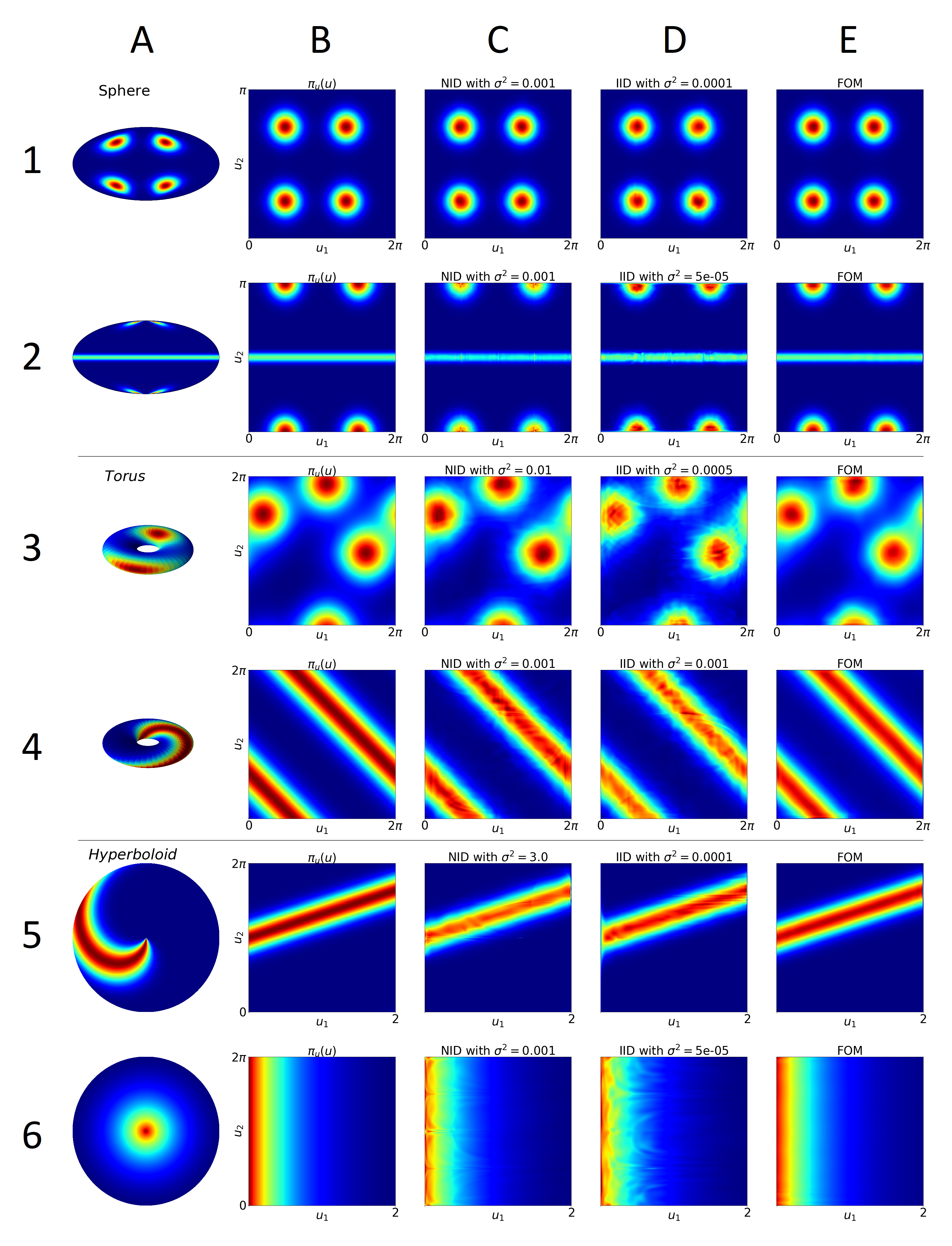
Figure 9: Columns A and B: Target density in data (A) and latent space (B) for various manifolds and different latent distributions. Column C: Best learned density using our method with NID. Column D: Best learned density using our method with IID. Column D: Learned density using FOM.

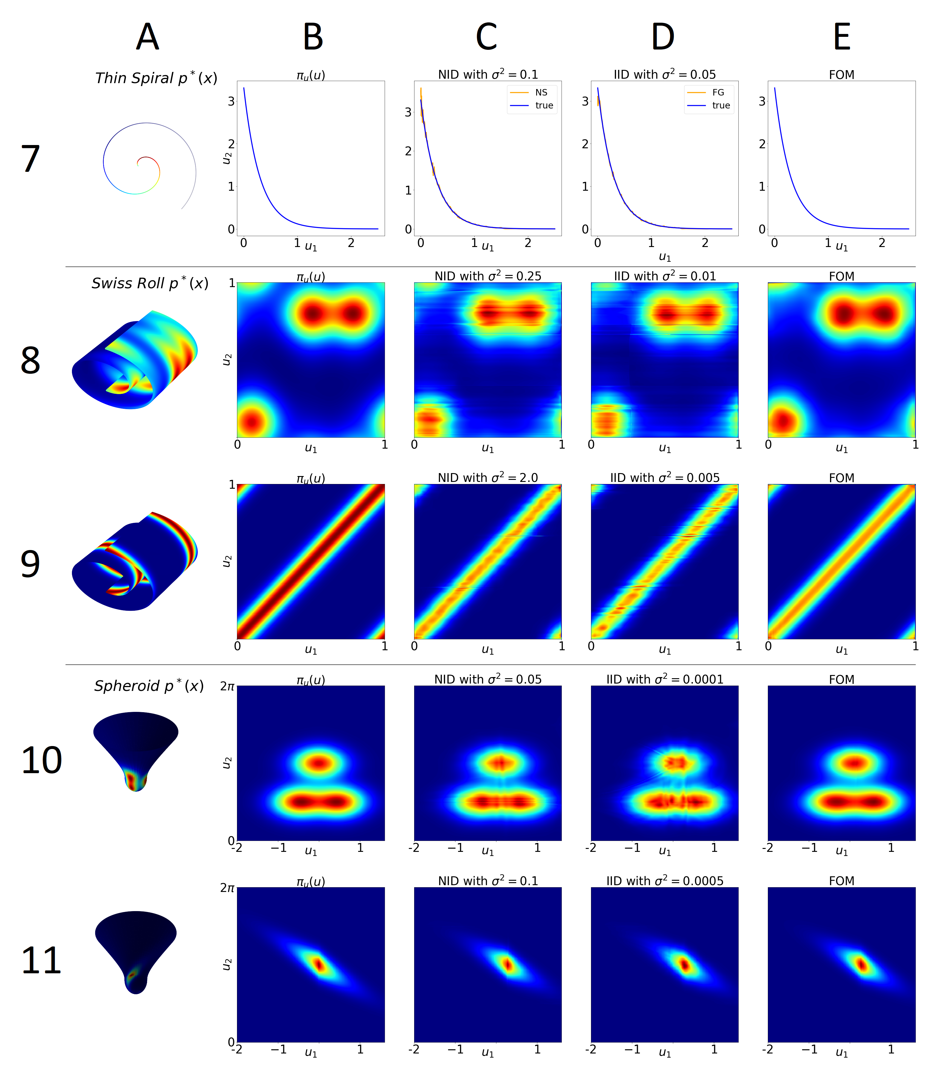
Figure 10: Columns A and B: Target density in data (A) and latent space (B) for various manifolds and different latent distributions. Column C: Best learned density using our method with NID. Column D: Best learned density using our method with IID. Column D: Learned density using FOM.

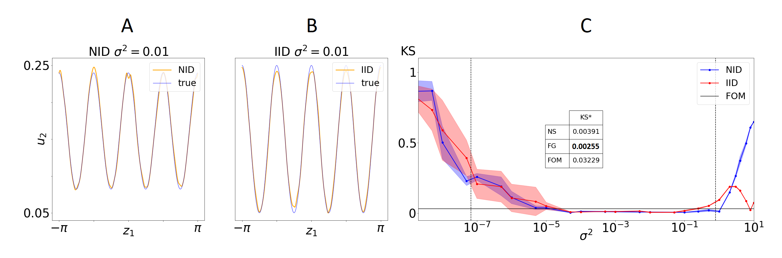
Figure 11: A: Learned latent density using NID (orange) on top of target latent density (blue). B: Learned latent density using IID (orange) on top of target latent density (blue). C: KS vs. $\sigma^{2}$ plot for IID and NID (we used 3 seeds for the error bars) with the KS value of FOM as horizontal line. Table in C: Optimal KS values for the different models. Vertical Lines in C: Lower and upper bound (see point 5. of the standard procedure).

B.4 Manifold Flow for the mixture of von Mises distributions on $S^{2}$

In this Subsection, we apply the manifold flow, see Section 4, on a mixture of von Mises distributions on a sphere. We do not attempt to find the optimal hyperparameters and training settings (such as batch- and training size, optimization method, or training scheduler) to maximize the performance.

The manifold flow (MF) proposed by Brehmer and Cranmer, 2020 uses two flows, one for encoding the data manifold to the latent space, and another for learning the latent density. To avoid calculating the Gram determinant of the encoding flow, they proposed different training procedures, an alternating, and a sequential (see Section 4 for more details). In Figure 13, we show that both methods learn the density reasonable good (top left and right). However, if we add Gaussian noise with magnitude $0.01$ to the dataset, the two training schemes lead to very different results (bottom left and right). This illustrates the drawback of not having a unified maximum likelihood objective. We used the same model and training settings as for a similar dataset (a two-dimensional manifold embedded in $\mathbb{R}^{3}$) studied in Brehmer and Cranmer, 2020.

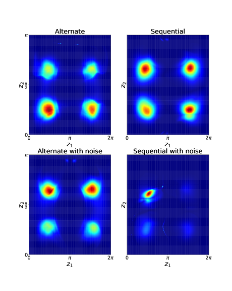
Figure 13: Performance of MF on the mixture of von Mises distributions on a sphere (top) and noisy sphere (bottom), using different training schemes (alternating left, and sequential right).

References

- Au and Tam (1999) Chi Au and Judy Tam. Transforming variables using the dirac generalized function. The American Statistician, 53(3):270–272, 1999. doi: 10.1080/00031305.1999.10474472. URL https://www.tandfonline.com/doi/abs/10.1080/00031305.1999.10474472.
- Beitler et al. (2018) Jan Jetze Beitler, Ivan Sosnovik, and Arnold Smeulders. Pie: Pseudo-invertible encoder. 2018.
- Berenfeld and Hoffmann (2019) Clément Berenfeld and Marc Hoffmann. Density estimation on an unknown submanifold. arXiv preprint arXiv:1910.08477, 2019.
- Brehmer and Cranmer (2020) Johann Brehmer and Kyle Cranmer. Flows for simultaneous manifold learning and density estimation. Advances in Neural Information Processing Systems, 33, 2020.
- Cunningham et al. (2020) Edmond Cunningham, Renos Zabounidis, Abhinav Agrawal, Ina Fiterau, and Daniel Sheldon. Normalizing flows across dimensions. arXiv preprint arXiv:2006.13070, 2020.
- De Cao et al. (2020) Nicola De Cao, Wilker Aziz, and Ivan Titov. Block neural autoregressive flow. In Uncertainty in Artificial Intelligence, pages 1263–1273. PMLR, 2020.
- Do Carmo (2016) Manfredo P Do Carmo. Differential geometry of curves and surfaces: revised and updated second edition. Courier Dover Publications, 2016.
- Durkan et al. (2019) Conor Durkan, Artur Bekasov, Iain Murray, and George Papamakarios. Neural spline flows. In Advances in Neural Information Processing Systems, pages 7511–7522, 2019.
- Facco et al. (2017) Elena Facco, Maria d’Errico, Alex Rodriguez, and Alessandro Laio. Estimating the intrinsic dimension of datasets by a minimal neighborhood information. Scientific reports, 7(1):1–8, 2017.
- Fefferman et al. (2016) Charles Fefferman, Sanjoy Mitter, and Hariharan Narayanan. Testing the manifold hypothesis. Journal of the American Mathematical Society, 29(4):983–1049, 2016.
- Feiten et al. (2013) Wendelin Feiten, Muriel Lang, and Sandra Hirche. Rigid motion estimation using mixtures of projected gaussians. In Proceedings of the 16th International Conference on Information Fusion, pages 1465–1472. IEEE, 2013.
- Geller (1997) Robert J Geller. Earthquake prediction: a critical review. Geophysical Journal International, 131(3):425–450, 1997.
- Gemici et al. (2016) Mevlana C Gemici, Danilo Rezende, and Shakir Mohamed. Normalizing flows on riemannian manifolds. arXiv preprint arXiv:1611.02304, 2016.
- Hamelryck et al. (2006) Thomas Hamelryck, John T Kent, and Anders Krogh. Sampling realistic protein conformations using local structural bias. PLoS Comput Biol, 2(9):e131, 2006.
- Hein and Audibert (2005) Matthias Hein and Jean-Yves Audibert. Intrinsic dimensionality estimation of submanifolds in rd. In Proceedings of the 22nd International Conference on Machine Learning, ICML ’05, page 289–296, New York, NY, USA, 2005. Association for Computing Machinery. ISBN 1595931805. doi: 10.1145/1102351.1102388. URL https://doi.org/10.1145/1102351.1102388.
- Huang et al. (2018) Chin-Wei Huang, David Krueger, Alexandre Lacoste, and Aaron Courville. Neural autoregressive flows. volume 80 of Proceedings of Machine Learning Research, pages 2078–2087, Stockholmsmässan, Stockholm Sweden, 10–15 Jul 2018. PMLR.
- Huang et al. (2020) Chin-Wei Huang, Laurent Dinh, and Aaron Courville. Augmented normalizing flows: Bridging the gap between generative flows and latent variable models. arXiv preprint arXiv:2002.07101, 2020.
- Kim et al. (2020) Hyeongju Kim, Hyeonseung Lee, Woo Hyun Kang, Joun Yeop Lee, and Nam Soo Kim. Softflow: Probabilistic framework for normalizing flow on manifolds. Advances in Neural Information Processing Systems, 33, 2020.
- Kingma and Dhariwal (2018) Diederik P Kingma and Prafulla Dhariwal. Glow: Generative flow with invertible 1x1 convolutions. arXiv preprint arXiv:1807.03039, 2018.
- Lecun et al. (1998) Y. Lecun, L. Bottou, Y. Bengio, and P. Haffner. Gradient-based learning applied to document recognition. Proceedings of the IEEE, 86(11):2278–2324, 1998. doi: 10.1109/5.726791.
- Lee (2019) J.M. Lee. Introduction to Riemannian Manifolds. Graduate Texts in Mathematics. Springer International Publishing, 2019.
- Loshchilov and Hutter (2016) Ilya Loshchilov and Frank Hutter. Sgdr: Stochastic gradient descent with warm restarts. arXiv preprint arXiv:1608.03983, 2016.
- Loshchilov and Hutter (2017) Ilya Loshchilov and Frank Hutter. Decoupled weight decay regularization. arXiv preprint arXiv:1711.05101, 2017.
- Lou et al. (2020) Aaron Lou, Derek Lim, Isay Katsman, Leo Huang, Qingxuan Jiang, Ser-Nam Lim, and Christopher De Sa. Neural manifold ordinary differential equations. arXiv preprint arXiv:2006.10254, 2020.
- Mathieu and Nickel (2020) Emile Mathieu and Maximilian Nickel. Riemannian continuous normalizing flows. arXiv preprint arXiv:2006.10605, 2020.
- Rezende and Mohamed (2015) Danilo Rezende and Shakir Mohamed. Variational inference with normalizing flows. In International Conference on Machine Learning, pages 1530–1538. PMLR, 2015.
- Rezende et al. (2020) Danilo Jimenez Rezende, George Papamakarios, Sébastien Racaniere, Michael Albergo, Gurtej Kanwar, Phiala Shanahan, and Kyle Cranmer. Normalizing flows on tori and spheres. In International Conference on Machine Learning, pages 8083–8092. PMLR, 2020.
- Zhang et al. (2020) Han Zhang, Xi Gao, Jacob Unterman, and Tom Arodz. Approximation capabilities of neural ODEs and invertible residual networks. In Hal Daumé III and Aarti Singh, editors, Proceedings of the 37th International Conference on Machine Learning, volume 119 of Proceedings of Machine Learning Research, pages 11086–11095. PMLR, 13–18 Jul 2020. URL https://proceedings.mlr.press/v119/zhang20h.html.