Abstract

Quasiclassical methods are used to define dynamical tunneling times in models of quantum cosmological bounces. These methods provide relevant new information compared with the traditional treatment of quantum tunneling by means of tunneling probabilities. As shown here, the quantum dynamics in bounce models is not secure from reaching zero scale factor, re-opening the question of how the classical singularity may be avoided. Moreover, in the examples studied here, tunneling times remain small even for large barriers, highlighting the quantum instability of underlying bounce models.

1 Introduction

A possible scenario of cosmological dynamics that avoids the classical big-bang singularity is given by bounces in modified or quantized models of gravity. If matter or gravity behave non-classically at high curvature, their features may present a barrier to evolution such that unbounded curvature or zero scale factor of an isotropic model are not reached. Instead, the scale factor may approach a non-zero constant value asymptotically, or it may bounce back to macroscopic values after a moment of maximal collapse [1].

Most models of this kind are evaluated in a way that is essentially classical (or, in more precise terms, leading-order quasiclassical), modifying the Friedmann equation without directly representing it through quantum operators. While it is technically possible to evolve a quantum state within a spatially homogeneous model of quantum cosmology, the uncertain nature of quantum space-time physics makes it hard to extend such results to inhomogeneous perturbations, such as the curvature or density distribution relevant for determining the primordial state underlying the cosmic microwave background. Moreover, we hardly have any information about possible restrictions on the quantum state the universe may be in at early times. It is therefore unclear how significant properties of specific evolved wave functions can be, beyond what the leading-order quasiclassical dynamics of the scale factor in a modified Friedmann equation would provide.

A key property in which quantum dynamics differs from classical physics is given by the tunneling effect. In early-universe cosmology, this effect suggests that barriers to evolution as they may be used in bounce models are not absolute. Finite barriers may slow down evolution across the barrier, but they do not completely prevent it. A direct classical treatment of a simple modified Friedmann equation ignores the tunneling effect. It could therefore be possible that quantum evolution remains singular even if a first-order quasiclassical treatment might suggest a bounce. This question has been raised and analyzed in [2], in particular for models of loop quantum cosmology, using the method of Euclidean saddle points in order to estimate tunneling probabilities.

A direct quantum treatment by wave functions is available in quantum cosmology and would be sensitive to tunneling effects. However, the usual stationary setting familiar from quantum mechanics might miss crucial features of the essential dynamical nature of the early universe. Moreover, the collapse of a single universe is conceptually different from a scattering process of an extended stream of particles, as assumed in standard tunneling calculations. Given the unknown nature of the quantum state of the universe, reliable conclusions in quantum cosmology require a sufficiently large set of states, parameterized in a suitable way that does not assume specific physical properties.

Here, we introduce methods of non-adiabatic quantum dynamics to bounce models in early-universe cosmology. These methods have appeared independently in various fields [3, 4, 5, 6, 7, 8] and have recently been shown to capture details tunneling effects in extended quasiclassical formulations [9, 10, 11]. In particular, these methods reveal the entire process of tunneling and can be used to determine characteristic parameters such as tunneling times. (See for instance [12, 13, 14] for discussions of the concept of tunneling times.) In their present form, they rely on semiclassical approximations, but based on a systematic expansion that can be applied to higher than the leading orders often assumed in heuristic discussions of bounce models.

2 Models

Our analysis is based on an anharmonic reformulation of the Friedmann dynamics derived in [15, 16]. Starting with

$$\left(\frac{\dot{a}}{a}\right)^{2}=\frac{8\pi G}{3}\rho$$ (1)

for vanishing spatial curvature, we first replace $\dot{a}$ with its canonical momentum, $p_{a}=-(3/4\pi G)V_{0}a\dot{a}$ where $V_{0}$ is the coordinate volume of a finite region in space. Specifying the matter density $\rho$ as given by a free, massless scalar field $\phi$ with momentum $p_{\phi}$,

$$\rho=\frac{1}{2}\frac{p_{\phi}^{2}}{a^{6}}\,,$$ (2)

we then note that the Friedmann equation implies the expression

$$p_{\phi}(a,p_{a})=\pm\sqrt{\frac{3}{4\pi G}}|ap_{a}|$$ (3)

for $p_{\phi}$ quadratic in the canonical variables $a$ and $p_{a}$.

2.1 Harmonic systems

Hamilton’s equations generated by $p_{\phi}(a,p_{a})$ determine how $a$ and $p_{a}$ evolve with respect to the scalar value $\phi$ as a formal time parameter. The quadratic nature of (3) shows that this evolution is essentially harmonic, except for the absolute value taken for $ap_{a}$ which might suggest that the Hamiltonian is not strictly quadratic. However, since the sign of $ap_{a}$ is preserved by evolution generated by a Hamiltonian proportional to $ap_{a}$, $p_{\phi}$ may be replaced with a Hamiltonian of the form (3) in which the absolute value has been dropped. Upon quantization, one should then impose the condition that a given initial state is supported either on the positive or on the negative part of the spectrum of $ap_{a}$.

More generally, the quadratic nature is preserved by any canonical transformation of $(a,p_{a})$ in which the new configuration variable is related to $a$ by a power law. A convenient definition that absorbs some of the constant parameters introduces a class of new canonical variables $Q$ and $P$ by

$$|Q|=\frac{3(\ell_{0}a)^{2(1-x)}}{8\pi G(1-x)}\quad,\quad P=-\ell_{0}^{1+2x}a^{2x}\dot{a}$$ (4)

where $\ell_{0}=V_{0}^{1/3}$ and $x$ is a free parameter that determines a particular canonical transformation. The absolute value of $Q$ indicates that we may conveniently extend this variable to the full real range, including negative values, if we combine the dependence on the scale factor with a sign factor that determines the orientation of space. This choice simplifies quantization because it removes a boundary from the classical phase space.

Also transforming $\phi$ to

$$\lambda=\sqrt{16\pi G/3}\>|1-x|\phi$$ (5)

for a given $x$, we obtain the simple expression

$$H=p_{\lambda}=\pm|QP|$$ (6)

for the momentum of $\lambda$, identified with the Hamiltonian $H$ for evolution of $Q$ and $P$ with respect to $\lambda$.

So far, we have reformulated classical dynamics of a spatially flat, isotropic universe with a specific matter ingredient. A possible modification of this dynamics has been suggested by loop quantum cosmology [17, 18], in which the $\lambda$-Hamiltonian is no longer quadratic in canonical variables but instead given by

$$H_{\delta}=\pm\frac{|Q\sin(\delta P)|}{\delta}$$ (7)

where $\delta$ characterizes the magnitude of quantum effects. While this Hamiltonian is non-polynomial in canonical variables, it can be mapped to a linear expression if non-canonical basic variables are used that form a suitable Lie algebra. Many of the formal properties that characterize a harmonic system are then preserved.

Specifically, in addition to $Q$, we use the complex expression

$$J=Q\exp(i\delta P)$$ (8)

instead of the momentum $P$. The real and imaginary parts of $J$, together with $Q$, provide three real functions that, based on their mutual Poisson brackets

$$\{Q,{\rm Re}J\}=-\delta{\rm Im}J\quad,\quad\{Q,{\rm Im}J\}=\delta{\rm Re}J\quad,\quad\{{\rm Re}J,{\rm Im}J\}=\delta Q\,,$$ (9)

can be identified with the generators of the Lie algebra ${\rm sl}(2,{\mathbb{R}})$ [19]. (See also [20, 21, 22, 23, 24, 25] for appearances of this algebra or related versions in quantum cosmology.) In these variables, the Hamiltonian

$$H_{\delta}=\pm\frac{|{\rm Im}J|}{\delta}$$ (10)

is linear (again, up to the absolute value).

2.2 Analog oscillators

While the systems derived so far are harmonic in a formal sense, their Hamiltonians do not appear in standard form with a kinetic energy and a quadratic potential. It is easy to see that the Hamiltonian $H$ can be mapped to an inverted harmonic oscillator by a linear canonical transformation of $Q$ and $P$. The family $H_{\delta}$, however, is harder to bring to standard form in this way because it is not based on canonical variables.

We therefore apply a different procedure to bring the Hamiltonians closer to standard form, following [16]. Starting with the equations of motion they generate, we will determine suitable energy expressions together with additional constraints. For $H$, the canonical equations of motion with respect to $\lambda$ are given by

$$\dot{Q}=Q\quad\mbox{and}\quad\dot{P}=-P\,.$$ (11)

The first equation directly implies the second-order equation of motion $\ddot{Q}=\dot{Q}=Q$ which can also be obtained from the analog Hamiltonian

$$H_{\rm analog}=\frac{1}{2}(\pi^{2}-Q^{2})\,.$$ (12)

The momentum $\pi$ is distinct from the original momentum $P$, and it is constrained by the fact that $H_{\rm analog}$ implies $\pi=\dot{Q}$ while we also have $\dot{Q}=Q$ according to the original equations of motion. We can therefore express the original dynamics for $Q$ by the standard inverted harmonic oscillator (12), subject to the constraint $H_{\rm analog}=0$ imposed on initial values.

The Hamiltonian $H_{\delta}$ generates equations of motion for the algebra generators $Q$, ${\rm Re}J$ and ${\rm Im}J$:

$$\dot{Q}={\rm Re}J$$ (13)

and

$$\frac{{\rm d}{\rm Re}J}{{\rm d}\lambda}=Q\,.$$ (14)

The third equation of motion simply states that ${\rm Im}J$ is conserved. While (11) is modified, we have the same second-order equation as before, $\ddot{Q}=Q$. Therefore, we may use the same analog Hamiltonian (12). However, since $\dot{Q}\not=Q$ now, there is no constraint that determines the value of $H_{\rm analog}$. There is now an independent momentum $\pi$ canonically conjugate to $Q$ and not strictly related to it.

The brackets (9) show that we may use the equation

$$\pi=\frac{{\rm Re}J}{\delta^{2}H_{\delta}}$$ (15)

as an analog momentum, noting that ${\rm Im}J=-\delta H_{\delta}$ (up to a sign choice) is conserved for evolution generated by $H_{\delta}$. Therefore, $\pi=\delta^{-2}\dot{Q}/H_{\delta}$. If we define the analog Hamiltonian

$$H_{\rm analog}=\frac{1}{2}\left(\delta^{2}H_{\delta}\pi^{2}-\frac{1}{\delta^{2}H_{\delta}}Q^{2}\right)\,,$$ (16)

its Hamilton equations are equivalent to the equations of motion (13) and (14). A canonical transformation from $(Q,\pi)$ to

$$\tilde{Q}=\frac{Q}{\delta\sqrt{H_{\delta}}}\quad,\quad\tilde{\pi}=\delta\sqrt{H_{\delta}}\pi$$ (17)

(assuming, without loss of generality, $H_{\delta}>0$) brings this Hamiltonian to the standard form of the inverted harmonic oscillator.

The value of the momentum $\pi$ is not strictly determined by $Q$, but it is related to the Hamiltonian by a reality condition, based on the definition (8) of $J$ as a complex expression. This definition implies that

$$|J|^{2}=({\rm Re}J)^{2}+({\rm Im}J)^{2}=Q^{2}\,.$$ (18)

Therefore,

$$\delta^{2}\pi^{2}=\frac{({\rm Re}J)^{2}}{({\rm Im}J)^{2}}=\frac{Q^{2}}{({\rm Im}J)^{2}}-1=\frac{Q^{2}}{\delta^{2}H_{\delta}^{2}}-1$$ (19)

or

$$\tilde{\pi}^{2}=\tilde{Q}^{2}-H_{\delta}\,.$$ (20)

We obtain the value of the analog Hamiltonian given by

$$H_{\rm analog}=\frac{1}{2}\left(\tilde{\pi}^{2}-\tilde{Q}^{2}\right)=-\frac{1}{2}H_{\delta}=-\frac{1}{2}p_{\lambda}\,.$$ (21)

Since $p_{\lambda}$ is a free parameter, there is no sharp constraint on $H_{\rm analog}$ in this model.

For small $Q$, the behavior of the harmonic systems as models of quantum cosmology may be modified, depending on quantization ambiguities [16]. In particular, spatial discreteness may imply that the linear expression for $\ddot{Q}$ is replaced by $\ddot{Q}=Q^{2}{\rm sgn}Q$ once $Q$ is sufficiently small. The corresponding analog Hamiltonian has a cubic potential,

$$H_{\rm cubic}=\frac{1}{2}\tilde{\pi}^{2}-\kappa|\tilde{Q}|^{3}$$ (22)

with some constant $\kappa$. Since we are interested in quantum tunneling at small $Q$, our main tunneling analysis will be based on this Hamiltonian. In addition, because the power-law form may be subject to quantization choices, we will consider the examples of a quartic potential and an anharmonic potential with quadratic and quartic contributions. From now on, we will suppress tildes in the variables of $H_{\delta}$ to simplify the notation.

2.3 Quasiclassical extensions

The initial Hamiltonian $H=QP$ can easily be quantized to $\hat{H}=\frac{1}{2}(\hat{Q}\hat{P}+\hat{P}\hat{Q})$, choosing a standard symmetric ordering. Quasiclassical formulations based on canonical effective equations consider evolution generated by an effective Hamiltonian $H_{\rm eff}=\langle\hat{H}\rangle$ in a suitable class of states used to compute the expectation value.

For a quadratic Hamilton operator, the effective Hamiltonian can be derived for any state, provided the latter is given not by a wave function but by a collection of expectation values and moments with respect to a set of basic operators, $\hat{Q}$ and $\hat{P}$ in our case. We therefore describe a (possibly mixed) state by an infinite set of numbers,

$$Q=\langle\hat{Q}\rangle\quad,\quad P=\langle\hat{P}\rangle$$ (23)

and central moments

$$\Delta(Q^{a}P^{b})=\langle(\hat{Q}-\langle\hat{Q}\rangle)^{a}(\hat{P}-\langle\hat{P}\rangle)^{b}\rangle_{\rm symm}$$ (24)

in completely symmetric (or Weyl) ordering, for any positive integers $a$ and $b$ such that $a+b>1$.

Expressed in these variables, our effective Hamiltonian reads

$$H_{\rm eff}(Q,P,\Delta(QP))=QP+\Delta(QP)\,.$$ (25)

We need a Poisson bracket in order to generate Hamilton’s equations. The definition [26, 27]

$$\{\langle\hat{A}\rangle,\langle\hat{B}\rangle\}=\frac{\langle[\hat{A},\hat{B}]\rangle}{i\hbar}\,,$$ (26)

combined with the Leibniz rule to apply it to products of expectation values as they appear in moments, fulfills all the requirements for a Poisson bracket. Moreover, it is easy to see that the usual evolution equations of quantum mechanics (in Schrödinger or Heisenberg form) are equivalent to Hamilton’s equations generated by $H_{\rm eff}=\langle\hat{H}\rangle$ for basic expectation values and moments.

Following this procedure, the present example of (25) yields the equations of motion

$$\dot{Q}=Q\quad,\quad\dot{P}=-P$$ (27)

without quantum corrections, accompanied by equations of motion

$$\frac{{\rm d}\Delta(Q^{2})}{{\rm d}\lambda} = 2\Delta(Q^{2})$$

$$\frac{{\rm d}\Delta(QP)}{{\rm d}\lambda} = 0$$

$$\frac{{\rm d}\Delta(P^{2})}{{\rm d}\lambda} = -2\Delta(P^{2})$$

as well as equations for higher-order moments. These equations can easily be solved, determining how a state spreads out as $Q$ changes.

Unlike basic expectation values, which preserve the classical Poisson bracket $\{Q,P\}=1$, moments are not canonical. (Their Poisson brackets are in general quadratic in moments; see [27, 28].) The moment term in (25) therefore does not provide an intuitive picture as given by the usual form of potentials in a Hamiltonian with a standard kinetic energy. In this situation, it is convenient to transform moments to new canonical coordinates, whose local existence is guaranteed by the Casimir–Darboux theorem [29, 30]. While it may in general be hard to derive such coordinates, for second-order moments they have been found several times independently [3, 4, 5, 6, 7, 8] (without drawing a connection with Poisson geometry): A canonical pair $(s,p_{s})$ such that $\{s,p_{s}\}=1$ together with the conserved quantity $U$ (a Casimir function that has vanishing Poisson brackets with any other function) produce the correct brackets of second-order moments if the latter are defined as

$$\Delta(Q^{2}) = s^{2}$$ (28)

$$\Delta(QP) = sp_{s}$$ (29)

$$\Delta(P^{2}) = p_{s}^{2}+\frac{U}{s^{2}}\,.$$ (30)

The uncertainty relation implies that $U$ is bounded from below by $\hbar^{2}/4$.

In these variables, our effective Hamiltonian is given by

$$H_{\rm eff}(Q,P,s,p_{s})=QP+sp_{s}\,.$$ (31)

It generates equations of motion that can be used to construct an extended version of the analog harmonic oscillator if we simply copy the previous procedure for the new canonical pair:

$$H_{\rm analog,eff}=\frac{1}{2}\left(\pi^{2}-Q^{2}+\pi_{s}^{2}-s^{2}\right)\,.$$ (32)

Also the constraint $\pi=Q$ has to be doubled, accompanied by $\pi_{s}=s$. Therefore, the two energy contributions from $(\pi,Q)$ and $(s,\pi_{s})$ have to vanish independently.

Notice that the effective analog Hamiltonian (32) differs from a standard effective formulation of the original analog Hamiltonian (12) in that it does not contain a term of the form $U/s^{2}$, as it would be expected if $\pi^{2}$ were treated as an expectation value $\langle\hat{\pi}\rangle^{2}+\Delta(\pi^{2})$ of the kinetic energy, followed by an application of the mapping (28) with $\pi$ instead of $P$. The reason for this difference is the fact that $\pi$ is not an independent momentum, owing to the constraint $\pi=Q$.

The analog Hamiltonian of $H_{\delta}$, however, is not subject to a sharp constraint, such that the momentum $\pi$ remains independent. We can therefore insert a $\pi$-version of (28) in the analog Hamiltonian, producing

$$H_{\delta,{\rm analog,eff}}=\frac{1}{2}\left(\pi^{2}+p_{s}^{2}+\frac{U}{s^{2}}-Q^{2}-s^{2}\right)\,.$$ (33)

For small $Q$, the quadratic potential is replaced by a cubic one that contains an absolute value. This potential is therefore not differentiable at $Q=0$, preventing us from using an expansion

$$\langle\hat{Q}^{3}\rangle=\langle(Q+\widehat{\Delta Q})^{3}\rangle=Q^{3}+3Q\Delta(Q^{2})+\Delta(Q^{3})$$ (34)

of a differential cubic term, where $\widehat{\Delta Q}=\hat{Q}-Q$ such that $\langle\widehat{\Delta Q}\rangle=0$. An extension to non-differential potentials $V(Q)$ has been given by [10] in the form

$$V_{\rm all-order}(Q,s)=\frac{1}{2}\left(\frac{U}{s^{2}}+V(Q+s)+V(Q-s)\right)$$ (35)

based on a moment-closure condition that assumes a specific dependence of higher-order moments on a single quantum variable, $s$. A similar potential can also be derived from the Wigner function if additional conditions of semiclassical behavior are imposed [31].

In cases in which $V(Q)$ is smooth, a comparison of a Taylor expansion of the $V$-terms in (35) with the Taylor expansion of a generic effective potential,

$$V_{\rm eff}(Q,\Delta(Q^{n})) = \langle V(\hat{Q})\rangle=\langle V(Q+\widehat{\Delta Q})\rangle$$ (36)

$$= V(Q)+\sum_{n=2}^{\infty}\frac{1}{n!}\frac{\partial^{n}V(Q)}{\partial Q^{n}}\Delta(Q^{n})\,,$$

shows that (35) is implied by (36) if the moments are such that $\Delta(Q^{n})=0$ for odd $n$, while $\Delta(Q^{n})=s^{n}$ for even $n$. Odd-order moments therefore do not contribute to (35) for smooth potentials, but they do in our case of a non-differentiable potential because $\frac{1}{2}\left(|Q+s|^{3}+|Q-s|^{3}\right)$ contains cubic contributions from $s$, which can easily be seen by evaluating the expression at $Q=0$. The full dependence of the polynomial effective potential

$$W(Q,s)=\frac{1}{2}\left(V(Q+s)+V(Q-s)\right)$$ (37)

on $Q$ and $s$ is illustrated in Fig. 1 for the cubic case.

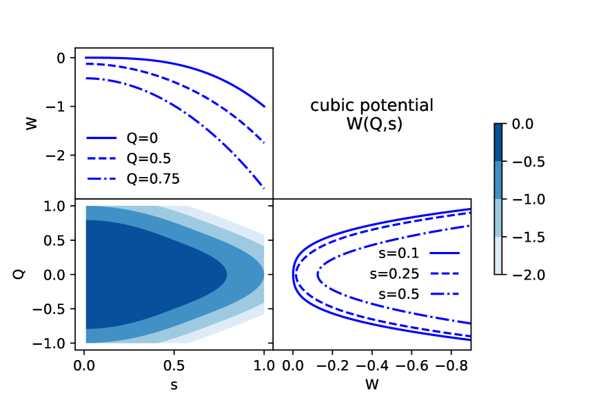
Figure 1: Visualization of the all-orders cubic potential with $\kappa=1$. A contour plot of the potential $W(Q,s)$ is shown at the bottom left, while cross-sections at constant $Q$ (top left) and constant $s$ (bottom right), respectively, are appended along the $s$ and $Q$ axes.

We relax the moment closure by introducing a free parameter, $a$, such that $\Delta(Q^{3})=as^{3}$ and writing the effective Hamiltonian as

$$H_{\rm cubic,eff}=\frac{1}{2}\pi^{2}+\frac{1}{2}p_{s}^{2}+\frac{U}{2s^{2}}-\kappa|Q|^{3}-3\kappa Qs^{2}-\kappa as^{3}\,.$$ (38)

The new parameter gives us more freedom to test the influence of the specific state on the tunneling behavior.

A quartic or anharmonic potential, which may be relevant if quantization ambiguities are taken into account, can be handled more easily because it is smooth. The corresponding effective Hamiltonians are

$$H_{\rm quartic,eff}=\frac{1}{2}\pi^{2}+\frac{1}{2}p_{s}^{2}+\frac{U}{2s^{2}}-\kappa Q^{4}-6\kappa Q^{2}s^{2}-4\kappa aQs^{3}-\kappa bs^{4}$$ (39)

and

$$H_{\rm anharmonic,eff}=\frac{1}{2}\pi^{2}+\frac{1}{2}p_{s}^{2}+\frac{U}{2s^{2}}-\frac{1}{2}\omega^{2}(Q^{2}+s^{2})-\kappa Q^{4}-6\kappa Q^{2}s^{2}-4\kappa aQs^{3}-\kappa bs^{4}\,,$$ (40)

respectively, where $a$ controls the cubic moment, as before, while $b$ plays a similar role for the quartic moment assumed to be of the form $\Delta(Q^{4})=bs^{4}$. The polynomial parts of these two potentials, given in the case of $a=0$ and $b=1$ by (37) applied to a quartic and anharmonic $V$, respectively, are shown in Figs. 2 and 3.

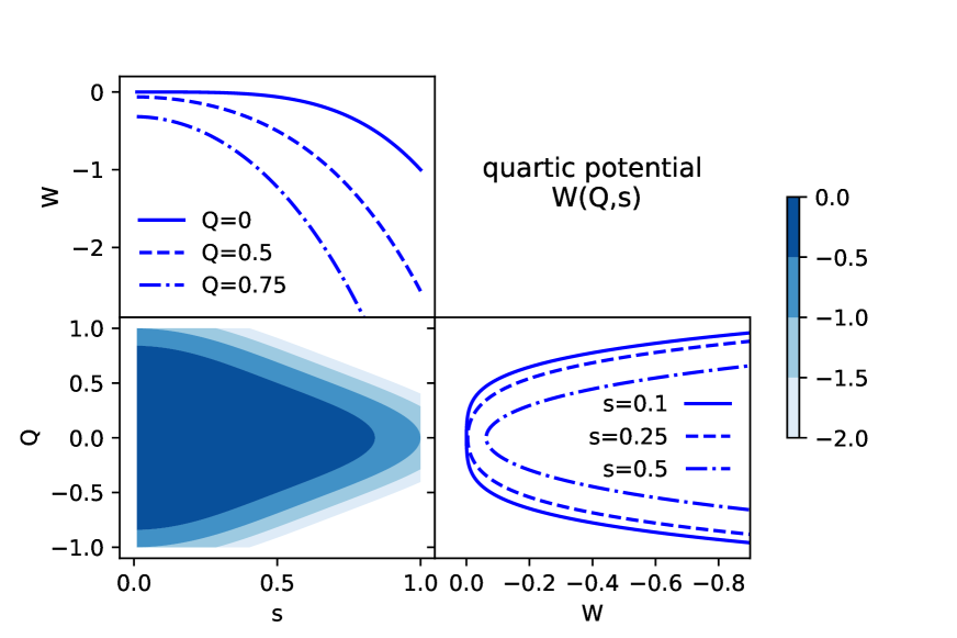
Figure 2: Visualization of the all-orders quartic potential with $\kappa=1$, using the method described in Fig. 1.

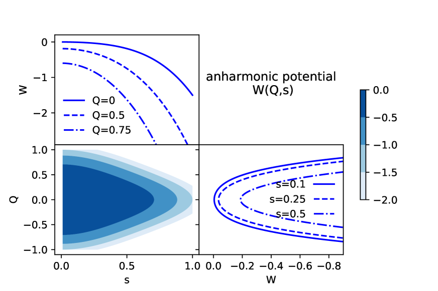
Figure 3: Visualization of an all-orders anharmonic potential with $\omega=\kappa=1$, using the method described in Fig. 1.

3 Tunneling dynamics

Our effective potentials allow us to study various properties of evolving quantum states while they are tunneling. As suggested by (21), the conserved energies in the quasiclassical models described by our effective analog Hamiltonians are negative, while their potentials vanish at $Q=0$. In each case, we therefore have a classical barrier that prevents $Q$ from changing sign as it evolves. A reflection of $Q$ at its turning point corresponds to a bounce in the quantum cosmological model represented by the analog system. Quantum mechanically, however, tunneling is possible and may replace a classical-type bounce with a transition through the singularity at $Q=0$.

The variable $Q$ in a quasiclassical formulation represents the expectation value of an operator $\hat{Q}$ in an evolving state. A zero value of $Q$ does not necessarily imply that the state is given by a wave packet centered around the singularity. More likely in a tunneling scenario, the expectation value might vanish because the wave function has split into two separate packets, one that stays on the side of the barrier where the initial wave function was set up, and one that has tunneled through the barrier. A vanishing expectation value $Q$ therefore may not lead to as strong a singularity as in the classical treatment. In this way, tunneling through the barrier could be similar to a strict bounce behavior in which the wave function always stays on one side of the barrier. Nevertheless, it is important to understand possible tunneling dynamics as a first step in an analysis of the transition, eventually with an inclusion of anisotropy and inhomogeneity. Some of the relevant degrees of freedom may well be affected by tunneling through $Q=0$ even if the zero may refer only to an expectation value and not necessarily to the support of a wave function. This possibility so far has not been considered in the literature.

While an inclusion of anisotropy and inhomogeneity would be well beyond the scope of the present paper, we proceed with a specific analysis of some dynamical tunneling properties in our isotropic analog models. In particular, we will focus on the question of how long it takes for a state to tunnel through the classical barrier. The usual treatment of tunneling in quantum mechanics, based on stationary states, does not reveal much about the actual process. In a quasiclassical model, however, tunneling time is well defined because we are able to track the evolving $Q$ and to check under which conditions and for how long it moves through the range determined by the classical barrier for a given energy. We will refer to this tunneling time as $\Delta t_{\rm evolution}$. As shown by Figs. 1–3, the effective potentials decrease in the $s$-direction around local maxima of the classical potential. Therefore, it is possible for certain trajectories to move around the classical barrier in the $(Q,s)$-plane while maintaining the initial energy.

Just as there is usually a non-zero reflection coefficient in the standard treatment of tunneling, some of the quasiclassical trajectories do not move around the barrier. We are interested in cases in which tunneling happens predominantly, which requires a specific choice of initial values for $Q$, $s$ and their momenta. In order to ensure that a given trajectory tunnels, we pose initial values at $Q=0$, at the maximum of the classical barrier. A given negative energy value then requires a minimum value of $s$ for real momenta to be possible. We choose an allowed value for $s$, set $p_{s}=0$ at the initial time and solve the analog energy equation for $\pi$. A complete set of initial values is thus obtained which can be integrated numerically, using equations of motion generated by the corresponding effective Hamiltonian. The time $\Delta t_{\rm evolution}$ required to cross the barrier can be read off from the resulting trajectory.

Before we discuss our specific results, we point out that the time parameter $t$ that appears in our tunneling times refers to evolution generated through Hamilton’s equations by an analog Hamiltonian. In general, this time is not the proper time of the cosmological model described in analog form. Since we are interested here in qualitative features of tunneling times, as in the example that follow, a transformation from $t$ to proper time is not required.

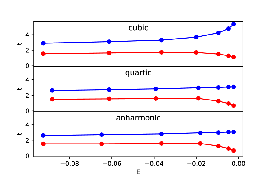
Figure 4: Tunneling times for various potentials, using two different methods. The red curves show our results obtained from evolution in a quasiclassical model. The blue curves show an alternative definition (41) based on integrating ${\rm d}t=(m/|p(Q)|){\rm d}Q$ across the classical barrier, using the imaginary momentum $p(Q)$. While both definitions lead to comparable orders of magnitude, their trends in particular at small energies are markedly different. The quasiclassical tunneling time does not significantly depend on the specific potential.

Our results are shown in Figs. 4 and 5. Figure 4 demonstrates that the dependence of tunneling times on the energy does not significantly depend on the specific low-order polynomial potential. Interestingly, this feature is not shared by alternative definitions of tunneling times, in particular at small absolute values of the energy, close to the top of the barrier. The figure shows one alternative method for comparison, given by a more traditional proposal [12, 13, 14] to estimate the tunneling time by the integral

$$\Delta t_{\rm integration}=\frac{1}{\sqrt{2}}\int_{Q_{-}}^{Q_{+}}\frac{\sqrt{m}{\rm d}Q}{\sqrt{V(Q)-E}}$$ (41)

where $Q_{\pm}$ are the classical turning points for the potential $V(Q)$ at energy $E$. This definition assumes that the imaginary part of the solution for $p$ of the energy equation $E=(2m)^{-1}p^{2}+V(Q)$ under the barrier may provide a reasonable estimate for $m{\rm d}Q/{\rm d}t$.

As our figure shows, the order of magnitute is close to our more detailed tunneling time based on quasiclassical evolution, but it is rather different at small energies, close to the top of the barrier of our potential. The evolution time clearly approaches zero as the energy gets closer to the top of the barrier because the required distance to travel eventually vanishes and momenta stay finite. But while the integration range in (41) also shrinks as $Q_{-}\to Q_{+}$ when $E$ approaches zero, the integrand gets bigger because it diverges at the turning points. This trend is particularly clear for the cubic potential in Fig. 4.

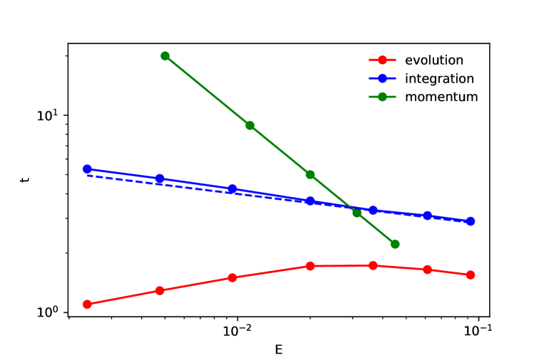
Figure 5: Tunneling times for the cubic potential in logarithmic display, showing results from quasiclassical evolution (red), integration of ${\rm d}t=(m/|p(Q)|){\rm d}Q$ (blue), and a simple estimate $m\Delta Q/p_{0}$ based on the momentum $p_{0}$ at the maximum of the barrier of width $\Delta Q$ (green). The blue dashed line is not a fit but has been included for orientation, showing the curve $t(E)=2E^{-0.15}$ for comparison.

The logarithmic plot of Fig. 5, shown only for the cubic potential, confirms this behavior. While the integration time, by inspection, is close to a power law $t(E)\sim 2E^{-0.15}$, the evolution time is not of power-law form and exhibits a more complicated behavior. In addition to these two definitions, the figure also shows a rough estimate of the tunneling time,

$$\Delta t_{\rm momentum}=\frac{m\Delta Q}{p_{0}}$$ (42)

based on the width $\Delta Q=Q_{+}-Q_{-}$ of the barrier and the momentum $p_{0}$ at $Q=0$ obtained from a given energy in a quasiclassical model. (The value of $p_{0}$ would be used as an initial condition in the more precise definition of tunneling times by complete evolution.) This behavior is of power-law form and does not agree with any one of the other two definitions. The precise evolution of a quasiclassical model is therefore relevant, and not just the fact that the energy can be above the potential for sufficiently large $s$. The latter feature, which guarantees that a real $p_{0}$ is obtained at $Q=0$, is shared by the evolution time and the momentum time, and yet the two results are different in many respects.

4 Discussion and implications for quantum cosmology

We have analyzed a detailed definition of tunneling time in analog models of quantum cosmological bounces. The analog method allowed us to model dynamics initially given for variables of an ${\rm sl}(2,{\mathbb{R}})$ algebra in terms of standard Hamiltonians. The Hamiltonians being of standard form, given by a kinetic energy quadratic in the momentum and a low-order polynomial potential, it becomes possible to construct a direct application of methods developed for quantum mechanics. In a second step, we applied quasiclassical formulations of non-adiabatic quantum dynamics in order to reveal crucial dynamical features of quantum evolution.

Our analysis revealed several properties of relevance for quantum cosmology. In particular, we showed that the definition of tunneling time based on non-adiabatic evolution of expectation values and moments of a state, unlike other and more traditional definitions, leads to small tunneling times near the top of the barrier. Moreover, as the energy decreases and the barrier becomes larger, the tunneling time plateaus or even starts decreasing as seen easily in the logarithmic plot of Fig. 5. Even a large barrier, therefore, does not present an effective way to stabilize bounce models dynamically. A classical barrier around the singularity does not suffice to prevent a dynamical transition through the singularity.

Whether this transition can re-introduce singular effects for instance in the dynamics of anisotropy or inhomogeneity remains an important open question. The variable $Q$ in a quasiclassical model represents the expectation value of the volume operator. The value zero may be reached for various reasons in terms of an underlying wave function, for instance by a wave function centered at zero or by a suitable superposition of two wave packets centered at non-zero values even if their support does not include zero. Which possibility is generically realized could be revealed by a detailed analysis of the fluctuation variable, $s$, in quasiclassical models. Our preliminary examples usually require a large value of $s$ at $Q=0$ because the effective potential has to drop down sufficiently far in the $s$-direction to give way for the quasiclassical trajectory. However, the required minimum of $s$ depends on the energy, which in turn depends on detailed quantum parameters of the underlying cosmological model. Different versions of tunneling wave functions may therefore be realized.

References

- [1] M. Novello and S. E. P. Bergliaffa, Bouncing cosmologies, Phys. Rep. 463 (2008) 127–213
- [2] A. T. Mithani and A. Vilenkin, Instability of an emergent universe, JCAP 05 (2014) 006, [arXiv:1403.0818]
- [3] R. Jackiw and A. Kerman, Time Dependent Variational Principle And The Effective Action, Phys. Lett. A 71 (1979) 158–162
- [4] F. Arickx, J. Broeckhove, W. Coene, and P. van Leuven, Gaussian Wave-packet Dynamics, Int. J. Quant. Chem.: Quant. Chem. Symp. 20 (1986) 471–481
- [5] R. A. Jalabert and H. M. Pastawski, Environment-independent decoherence rate in classically chaotic systems, Phys. Rev. Lett. 86 (2001) 2490–2493
- [6] O. Prezhdo, Quantized Hamiltonian Dynamics, Theor. Chem. Acc. 116 (2006) 206
- [7] T. Vachaspati and G. Zahariade, A Classical-Quantum Correspondence and Backreaction, Phys. Rev. D 98 (2018) 065002, [arXiv:1806.05196]
- [8] M. Mukhopadhyay and T. Vachaspati, Rolling with quantum fields, [arXiv:1907.03762]
- [9] B. Baytaş, M. Bojowald, and S. Crowe, Faithful realizations of semiclassical truncations, Ann. Phys. 420 (2020) 168247, [arXiv:1810.12127]
- [10] B. Baytaş, M. Bojowald, and S. Crowe, Effective potentials from canonical realizations of semiclassical truncations, Phys. Rev. A 99 (2019) 042114, [arXiv:1811.00505]
- [11] B. Baytaş, M. Bojowald, and S. Crowe, Canonical tunneling time in ionization experiments, Phys. Rev. A 98 (2018) 063417, [arXiv:1810.12804]
- [12] E. H. Hauge and J. A. Stovneng, Tunneling times: a critical review, Rev. Mod. Phys. 61 (1989) 917–936
- [13] R. Landauer and Th. Martin, Barrier interaction time in tunneling, Rev. Mod. Phys. 66 (1994) 217–228
- [14] U. S. Sainadh, R. T. Sang, and I. V. Litvinyuk, Attoclock and the quest for tunnelling time in strong-field physics, J. Phys. Photonics 2 (2020) 042002
- [15] M. Bojowald, Harmonic cosmology: How much can we know about a universe before the big bang?, Proc. Roy. Soc. A 464 (2008) 2135–2150, [arXiv:0710.4919]
- [16] M. Bojowald, Non-bouncing solutions in loop quantum cosmology, JCAP 07 (2020) 029, [arXiv:1906.02231]
- [17] M. Bojowald, Loop Quantum Cosmology, Living Rev. Relativity 11 (2008) 4, [gr-qc/0601085], http://www.livingreviews.org/lrr-2008-4
- [18] M. Bojowald, Quantum cosmology: a review, Rep. Prog. Phys. 78 (2015) 023901, [arXiv:1501.04899]
- [19] M. Bojowald, Large scale effective theory for cosmological bounces, Phys. Rev. D 75 (2007) 081301(R), [gr-qc/0608100]
- [20] E. R. Livine and M. Martín-Benito, Group theoretical Quantization of Isotropic Loop Cosmology, Phys. Rev. D 85 (2012) 124052, [arXiv:1204.0539]
- [21] J. Ben Achour and E. Livine, The Thiemann Complexifier and the CVH algebra for Classical and Quantum FLRW Cosmology, Phys. Rev. D 96 (2017) 066025, [arXiv:1705.03772]
- [22] J. Ben Achour and E. Livine, Polymer Quantum Cosmology: Lifting quantization ambiguities using a conformal symmetry, Phys. Rev. D 99 (2019) 126013, [arXiv:1806.09290]
- [23] J. Ben Achour and E. Livine, Protected Symmetry in Quantum Cosmology, JCAP 09 (2019) 012, [arXiv:1904.06149]
- [24] N. Bodendorfer and F. Haneder, Coarse graining as a representation change, Phys. Lett. B 792 (2019) 69–73, [arXiv:1811.02792]
- [25] N. Bodendorfer and D. Wuhrer, Renormalisation with SU(1, 1) coherent states on the LQC Hilbert space, [arXiv:1904.13269]
- [26] M. Bojowald and A. Skirzewski, Effective Equations of Motion for Quantum Systems, Rev. Math. Phys. 18 (2006) 713–745, [math-ph/0511043]
- [27] M. Bojowald and A. Skirzewski, Quantum Gravity and Higher Curvature Actions, Int. J. Geom. Meth. Mod. Phys. 4 (2007) 25–52, [hep-th/0606232], Proceedings of “Current Mathematical Topics in Gravitation and Cosmology” (42nd Karpacz Winter School of Theoretical Physics), Ed. Borowiec, A. and Francaviglia, M.
- [28] M. Bojowald, D. Brizuela, H. H. Hernandez, M. J. Koop, and H. A. Morales-Técotl, High-order quantum back-reaction and quantum cosmology with a positive cosmological constant, Phys. Rev. D 84 (2011) 043514, [arXiv:1011.3022]
- [29] V. I. Arnold, Mathematical Methods of Classical Mechanics, Springer, 1997
- [30] A. Cannas da Silva and A. Weinstein, Geometric models for noncommutative algebras, volume 10 of Berkeley Mathematics Lectures, Am. Math. Soc., Providence, 1999
- [31] E. J. Heller, Wigner phase space method: Analysis for semiclassical applications, J. Chem. Phys. 65 (1976) 1289–1298