A Remarkable Summation Formula, Lattice Tilings, and Fluctuations

Abstract.

We derive and prove an explicit formula for the sum of the fractional parts of certain geometric series. Although the proof is straightforward, we have been unable to locate any reference to this result.

This summation formula allows us to efficiently analyze the average behavior of certain common nonlinear dynamical systems, such as the angle-doubling map, $x\mapsto 2x$ modulo 1. In particular, one can use this information to analyze how the behavior of individual orbits deviates from the global average (called fluctuations). More generally, the formula is valid in $\mathbb{R}^{m}$, where expanding maps give rise to so-called number systems. To illustrate the usefulness in this setting, we compute the fluctuations of a certain map on the plane.

1 Introduction.

The aim of this note is to state and prove an explicit formula that expresses the sum of the fractional parts of certain geometric series and to demonstrate its usefulness. This formula (Theorem 3.3) and some of its corollaries are discussed in Section 3. In this introduction, we discuss an important, and intuitive, special case (Lemma 1.3). In Sections 2 and 5, we will use these results to better understand the statistical behavior of certain (expanding) dynamical systems.

Consider the map $T:[0,1)\rightarrow[0,1)$ defined by

$$T:x\rightarrow 2x\mod 1\,.$$ (1.1)

This is often called the angle doubling map, because it describes the dynamics restricted to the unit circle in the complex plane of $z\mapsto z^{2}$, [5]. The action of that map is that it doubles the angle. Thus repeated applications of $T$ tend to separate nearby initial points exponentially fast. For that reason, this map serves as a paradigm for chaotic dynamical systems. A convenient way to study the behavior of orbits under $T$ is to write the initial condition $x$ in base 2:

$$x=0.d_{1}d_{2}d_{3}\cdots=\sum_{i=1}^{\infty}\,2^{-i}d_{i}\,,$$ (1.2)

where each $d_{i}$ is either 0 or 1. It is easy to see that

$$T(x)=0.d_{2}d_{3}d_{4}\cdots\quad\textrm{and so}\quad T^{n}(x)=0.d_{n+1}d_{n+2}d_{n+3}\cdots\,.$$

In nonlinear dynamical systems such as this one, it is as a rule too much to ask for exact solutions. One often settles for studying average behavior, and, as we shall see later, the distribution of the deviations from the average.

So let us do some averaging. One checks that $\frac{3}{7}$, $\frac{6}{7}$, $\frac{5}{7}$ form an orbit of period 3 under $T$. The three points of the periodic orbit sum to 2, and so their average equals $\frac{2}{3}$. Now let us look at this in base 2. It is a simple exercise to show that the three points are

$$0.\overline{011}\quad 0.\overline{110}\quad 0.\overline{101}\,.$$

The overbar is used to indicate periodicity. So $0.\overline{011}$ indicates $0.011011011\cdots$. What we observe is that the average of the orbit equals the average of the number of ones in the binary expansion of the initial condition $x$. This is not a coincidence! We leave it to the reader to check the following example of period 5:

$$\frac{5}{31}\quad\frac{10}{31}\quad\frac{20}{31}\quad\frac{9}{31}\quad\frac{18}{31}\,.$$

In binary notation, this becomes

$$0.\overline{00101}\quad 0.\overline{01010}\quad 0.\overline{10100}\quad 0.\overline{01001}\quad 0.\overline{10010}\,.$$

Again, one checks that the average of the orbit equals the average number of ones in the binary expansion. For periodic orbits, this is actually pretty easy to see by formally summing the binary expressions of all the periodic points. We leave that as an exercise, and move on to a stronger statement.

We introduce the notation $p_{n}=\sum_{i=1}^{n}\,d_{i}$ to denote the running number of ones in the binary representation of $x$ in the digits 1 through n (to the right of the decimal point). Also, to get our notation closer to that of the general case, we write $\left\{2x\right\}$ for $T(x)$. The braces are standard notation for “fractional part”. So $T^{i}(x)$ becomes $\left\{2^{i}x\right\}$.

We will now give an informal proof of the following, perhaps surprising, fact that the average of $\left\{2^{i}x\right\}$ converges if and only if the average of $p_{n}$ does, and that the limits are equal. A more general statement with a complete proof will follow in Section 3.

Lemma 1.1

If the base 2 expansion of $x\in[0,1)$ does not end in all ones, then

$$\lim_{n\rightarrow\infty}\left(\frac{1}{n}\,\sum_{i=0}^{n-1}\,\left\{2^{i}x\right\}-\frac{p_{n}}{n}\right)=0\,.$$ (1.3)

F.or simplicity, let us set $x=\sum_{i=1}^{n}\,2^{-j}d_{j}$. We first establish the following equality:

$$\sum_{i=0}^{n-1}\,\left\{2^{i}x\right\}=p_{n}-x\,.$$ (1.4)

The crux is the observation that we can do the summation for each digit separately, and only after that add up the results. So for fixed $1\leq j\leq n$ this gives

$$\sum_{i=0}^{n-1}\,\left\{2^{i}2^{-j}d_{j}\right\}=\sum_{i=0}^{j-1}\,2^{i}2^{-j}d_{j}=\frac{2^{j}-1}{2-1}\;2^{-j}d_{j}=d_{j}-d_{j}2^{-j}\,.$$

(Note that in the first summation the fractional part of $2^{i}2^{-j}d_{j}$ is zero if $i\geq j$.) Summing over $j$ from 1 to $n$ now gives equation (1.4). The lemma then follows by taking an average of equation (1.4), and then taking the limit as $n$ tends to infinity.  

There is a problem with taking the limit in this proof if the expansion of $x$ ends in all ones, because the function $x\rightarrow\{x\}$ is not continuous as $x$ approaches 1 from the left. This will be overcome in the more general treatment in Section 3. For now, suffice it to say that the exceptional set is countable and so will not affect the statistical reasoning in Section 2.

Equation (1.4) has an amusing corollary. We know that $\sum_{i=0}^{n-1}\,2^{i}x=(2^{n}-1)x$. Since $\left[2^{i}x\right]=2^{i}x-\left\{2^{i}x\right\}$, we now obtain the following.

$$\sum_{i=0}^{n-1}\,\left[2^{i}x\right]=2^{n}x-p_{n}\,.$$ (1.5)

The reason we present these basic facts is twofold. First, the map $T$ is probably one of the most studied maps in mathematics, and yet, to our surprise, with one exception [16], we do not know of any explicit mention of these simple facts, including Lemma 1.3. Second, and no less important, these identities can be useful. In fact, (1.4) was employed in [16] to greatly simplify the characterization of the statistical properties of orbits of a one parameter family of piecewise linear circle maps (see Section 2).

For the interested reader, we remark that the study of the average behavior of typical orbits of a dynamical system is a branch of mathematics, called ergodic theory, with far-reaching consequences for physics [1]. It is natural and interesting to investigate the deviations from average behavior; such deviations are called fluctuations and have a history of hundreds of years. In the classical theory, one assumes or establishes statistical independence of certain events — coin tosses say — and from this one derives Gaussian distributions for the fluctuations. Some of the mathematical history can be found in the short, but delightful book [9]. The application of these ideas to physics form the basis for the sub-discipline of physics called statistical physics (see [12]).

Since the 1980s, however, Tsallis and others have noted that in systems with correlations over long distances — which make the system less chaotic — statistical independence might not hold (see [14][Chapters 5 and 7]). They proposed that fluctuations in such systems might typically have distributions that are not Gaussian, but a generalization thereof ([14][Section 3.2] and references therein). This is currently a very active area of research. In general, these fluctuations are very hard to analyze, in particular if they do not have a Gaussian distribution. However, recently two low-dimensional systems with non-Gaussian fluctuations have been analyzed. It is intriguing that one of them [3] seems to conform to the theory proposed, while the other does not [16].

2 Fluctuations in One Dimension.

Let $f$ be a map from the unit interval to itself. Consider

$$S(n,x):=\sum_{i=0}^{n-1}f^{i}(x)\,.$$

The fluctuations are defined as the deviations of the partial sums from the average. Let us assume, for simplicity, that the average of $f$ (over $x$) equals $1/2$. Then by fluctuations, we mean the distribution of

$$S(n,x)-\frac{n}{2}\,.$$

as $x$ varies uniformly over all initial conditions and parameters while holding $n$ fixed. We are interested in establishing whether a properly rescaled version of these fluctuations tends to a limiting distribution as $n$ tends to infinity.

An important generic example is the angle doubling map $T$ in the introduction.

$$S(n,x):=\sum_{i=0}^{n-1}\{2^{i}x\}\,.$$

Almost all $x\in[0,1)$ have a unique base 2 expansion. Thus Lemma 1.3 tells us what the result is. For large $n$, the distribution of $S$ tends to that of $\sum_{i=1}^{n}\,d_{i}$ because the contribution of $\left\{2^{n}x\right\}-x$ is negligible. The resulting distribution is of course the binomial one

$$\textrm{Prob}(S\leq k)=2^{-n}\sum_{x=0}^{k}\binom{n}{x}\,,$$

which has mean $\mu=\frac{n}{2}$ and standard deviation $\sigma=\frac{1}{2}\sqrt{n}$. It is well-known that for large $n$, the binomial distribution is increasingly well approximated by the Gaussian distribution $\frac{1}{\sigma\sqrt{2\pi}}\,\int_{-\infty}^{k}\,e^{-\frac{1}{2}\left(\frac{x-\mu}{\sigma}\right)^{2}}\,dx$. With $\mu$ and $\sigma$ as given above, we conclude that

$$\lim_{n\rightarrow\infty}\,\textrm{Prob}\left(\frac{2(S-\frac{n}{2})}{\sqrt{n}}\leq k\right)=\frac{1}{\sqrt{2\pi}}\,\int_{-\infty}^{k}\,e^{-\frac{1}{2}x^{2}}\,dx\,.$$ (2.6)

The derivative with respect to $k$ is the probability density $\frac{1}{\sqrt{2\pi}}\,e^{-\frac{1}{2}k^{2}}$ associated with the fluctuations (rescaled by $1/\sqrt{n}$).

In the above case, the conclusion is that the distribution of the fluctuations — upon appropriate rescaling — is Gaussian. This is expected for systems like $T$ that are expanding and therefore chaotic. However, the interesting cases, in view of Tsallis’ theory mentioned in the introduction, are those for which the fluctuations have a non-Gaussian distribution that can be analyzed exactly. Since there are very few of these, any explicit examples are very useful to gain intuition. We briefly present the example from [16].

Figure 2.1: Construction of a family of circle maps $f_{t}(x)$ given in (2.7) based on truncations of the angle doubling map. The horizontal axis is $x$. The vertical axis is $f_{t}(x)$.

We look at a family of maps that are considerably less chaotic, see Figure 2.1.

$$f_{t}(x)=\left\{\begin{matrix}t&\textrm{ for }0\leq x\leq\frac{t}{2}\\[2.84544pt] 2x&\textrm{ for }\frac{t}{2}\leq x\leq\frac{1}{2}\\[2.84544pt] 2x-1&\textrm{ for }\frac{1}{2}\leq x\leq\frac{1+t}{2}\\[2.84544pt] t&\textrm{ for }\frac{1+t}{2}\leq x\leq 1\end{matrix}\right.$$ (2.7)

Following [3, 16], in this case, we consider

$$S(n,t,x):=\sum_{i=0}^{n-1}f_{t}^{i}(x)\,,$$

and we define the fluctuations as the deviations of the partial sums from the average over $x$ and $t$. From symmetry considerations, one can see that this average is $1/2$. It is well-known that each of the maps $f_{t}$ has dynamics similar (in fact, semi-conjugate) to a pure rotation [16] (and references therein). That means that for each fixed value of $t$, each iterate of the map advances on average by a constant $\rho(t)\in[0,1]$, called the rotation number. It turns out that $\rho(t)$ is an increasing function of $t$. Points under $f_{t}$ rotate faster if $t$ is large. Thus iterations for different $t$ drift apart linearly in $n$. To get something that converges to a distribution, we will need to shift $S$ by the average $1/2$ and rescale by $1/n$. So we consider

$$\frac{1}{n}\left(S(n,t,x)-\frac{n}{2}\right)=\frac{1}{n}\,\sum_{i=0}^{n-1}\left(f_{t}^{i}(x)-\frac{1}{2}\right)\,,$$ (2.8)

where now both $t$ and $x$ are uniformly distributed over $[0,1)$ while $n$ is fixed but large. The hope is that the distribution of this tends (as $n\rightarrow\infty$) to a fixed non-trivial distribution.

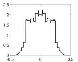
Figure 2.2: The probability density function for the fluctuations of the family of maps $f_{t}$.

The computations are now substantially more complicated, but an important step is again a summation to which Lemma 1.3 is applied. Here we can only give a very cursory idea how the proof goes. For the details, we refer to [16]. We need to average $S(n,t,x)$ in (2.8) over $x$ and $t$. It is sufficient to consider only cases where the rotation is rational (the rest has measure zero). So choose $t$ in the interval $I_{p/q}$ of values such that the rotation number of $f_{t}$ is equal to $\frac{p}{q}$ where $\gcd(p,q)=1$. With that choice, $x=t$ (see Figure 2.1) is a stable periodic orbit of period $q$ which attracts all initial conditions. From that one can derive that it essentially determines the sum in (2.8) for all $t\in I_{p/q}$. So, for large $n$

$$\frac{1}{n}\left(S\left(n,t,x\right)-\frac{n}{2}\right)\approx\frac{1}{q}\,\sum_{i=0}^{q-1}\left(\left\{2^{i}t\right\}-\frac{1}{2}\right)\,.$$

Lemma 1.3 is applied to evaluate this sum and average over $t\in I_{p/q}$ and over $x$. Finally, we obtain the overall probability density associated with the fluctuations as a sum over the rationals $\frac{p}{q}$ between 0 and 1. It can be computed numerically to arbitrary precision and has a remarkable (and very non-Gaussian) appearance as can be appreciated in Figure 2.2.

3 A Summation Formula.

In this section, we consider expansions in $\mathbb{R}^{m}$ that are generalizations of those in (1.2). The number $2$ in that equation is replaced by a matrix $A$ which is expanding (i.e. all eigenvalues have modulus greater than 1) and whose entries are integers so that $A\mathbb{Z}^{m}$ forms a sublattice of $\mathbb{Z}^{m}$. The determinant of $A$ is $\pm q$ for some integer $q$ greater than 1. This means that $A$ maps the unit cube $[0,1]^{m}$ to a parallelotope (an $m$ dimensional “parallelogram”) of volume $q$. Call two elements of $\mathbb{Z}^{m}$ equivalent if they differ by an element of $A\mathbb{Z}^{m}$. There are precisely $q$ equivalence classes of points in $\mathbb{Z}^{m}$. A set $D$ is a standard digit set if it contains exactly one element for each equivalence class. In number theoretic terms, $D$ corresponds to a complete set of residues modulo $A$. Without loss of generality, we require that $0\in D$. This is what is called a standard number system. We summarize the definition here.

Definition 3.1

A standard number system $(A,D)$ in $\mathbb{R}^{m}$ is given by an expanding matrix with integer coefficients $A$, a digit set $D$ of cardinality $q=|\det A|$ containing exactly one element of each coset of $A\mathbb{Z}^{m}$ in $\mathbb{Z}^{m}$, one of which is the origin.

Consider vectors in $\mathbb{R}^{m}$ of the following form

$$x=A^{\ell}d_{-\ell}+\cdots A^{0}d_{0}+A^{-1}d_{1}+A^{-2}d_{2}+\cdots=\sum_{i=-\ell}^{\infty}\,A^{-i}d_{i}\,,$$ (3.9)

where the digits $d_{i}$ in the above expression are chosen from a standard digit set $D$ and $d_{-\ell}\neq 0$. Since $A$ is expanding, $A^{-1}$ is well-defined with eigenvalues of modulus strictly smaller than 1, and so the sum in (3.9) converges exponentially.

Definition 3.2

For $x\in\mathbb{R}^{m}$ and an expansion ${\boldsymbol{d}}$ given by $x=\sum_{i=-\ell}^{\infty}\,A^{-i}d_{i}$, define the integer part $[x]$ and the fractional part $\{x\}$ as

$$[x({\boldsymbol{d}})]=\sum_{i=-\ell}^{0}\,A^{-i}d_{i}\quad\;\;{\rm and}\;\;\quad\{x({\boldsymbol{d}})\}=\sum_{i=1}^{\infty}\,A^{-i}d_{i}\,,$$ (3.10)

Denote the set of fractional parts by $\cal F$ and the set of integral parts by $\cal I$.

Remark. It is important to bear in mind that the definition above is different from the usual definition of integral and fractional parts in that these depend on the expansion ${\boldsymbol{d}}$ of $x$. For example, with this definition, $0.111\cdots$ (in base 2) has fractional part 1 and integral part 0, while $1.000\cdots$ has fractional part 0 and integral part 1.

It turns out that for the number systems in $\mathbb{R}^{m}$ that interest us, these cases have measure zero. Since we aim to do statistical calculations, we can safely neglect them. Some more details are given in Section 4. Because of this, and for notational convenience, we drop the dependence on the expansion from our notation, and write $\{x\}$ and $[x]$ from now on.

Now we get to our main results.

Theorem 3.3 (Fractional Part Summation Formula)

If $(A,D)$ is a standard number system, then for any $x\in\mathbb{R}^{m}$ with a base $A$ expansion $\sum_{i=-\ell}^{\infty}\,A^{-i}d_{i}$

$$(A-I)\,\sum_{i=0}^{n-1}\,\{A^{i}x\}=\sum_{i=1}^{n}\,d_{i}+\left\{A^{n}x\right\}-\{x\}\,.$$

F.irst, split up $\{x\}$ as follows

$$\{x\}=\sum_{i=1}^{n}\,A^{-i}d_{i}+\sum_{i=n+1}^{\infty}\,A^{-i}d_{i}:=x_{n}+y_{n}\,.$$ (3.11)

As in Lemma 1.3, one observes that the summation can be carried out for each digit separately, and then the result can be added up. So let us start with the digits in $x_{n}$. For a fixed $j\in\{1,\cdots,n\}$, using the fact that $A-I$ is invertible, we get

$$\sum_{i=0}^{n-1}\,\{A^{i}A^{-j}d_{j}\}=\sum_{i=0}^{j-1}\,A^{i}A^{-j}d_{j}=(A-I)^{-1}\,(A^{j}-I)\,A^{-j}d_{j}\,.$$

In the first equality, $A^{i}A^{-j}d_{j}$ are integer vectors for $i\geq j$, so their fractional parts are zero. Thus we can change the upper limit of the sum in order to remove $\{\cdot\}$. The second equality is a geometric series. Multiplying by $A-I$ and then summing over $j\in\{1,\cdots,n\}$ gives

$$(A-I)\sum_{i=0}^{n-1}\,\{A^{i}x_{n}\}=\sum_{j=1}^{n}\,d_{j}-x_{n}\,.$$

Since $\{A^{i}y_{n}\}=A^{i}y_{n}$ for all $0<i\leq n$, the remaining summation is also a geometric series:

$$(A-I)\sum_{i=0}^{n-1}\,\{A^{i}y_{n}\}=(A-I)\sum_{i=0}^{n-1}\,A^{i}y_{n}=(A^{n}-I)y_{n}\,.$$

Adding the last two displayed equations gives

$$(A-I)\sum_{i=0}^{n-1}\,\{A^{i}(x_{n}+y_{n})\}=\sum_{j=1}^{n}\,d_{j}+A^{n}y_{n}-x_{n}-y_{n}\,.$$

and noting that $x_{n}+y_{n}=\{x\}$ and $A^{n}y_{n}=\left\{A^{n}x\right\}$ gives the result.  

Corollary 3.4

If $(A,D)$ is a standard number system, then for any $x\in\mathbb{R}^{m}$ with a base $A$ expansion $\sum_{i=-\ell}^{\infty}\,A^{-i}d_{i}$

$$\lim_{n\rightarrow\infty}\left((A-I)\,\frac{1}{n}\,\sum_{i=0}^{n-1}\,\{A^{i}x\}-\frac{1}{n}\,\sum_{i=1}^{n}\,d_{i}\right)=0\,.$$

N.ote that in Theorem 3.3, $\{x\}$ and $\left\{A^{n}x\right\}$ are fractional numbers. Thus their modulus is less than some a priori bound. The corollary follows immediately upon dividing by $n$ and taking a limit as $n\rightarrow\infty$.  

Theorem 3.3 also has a curious corollary analogous to equation 1.5.

Corollary 3.5

If $(A,D)$ is a standard number system, then for any $x\in\mathbb{R}^{m}$ with a base $A$ expansion $\sum_{i=-\ell}^{\infty}\,A^{-i}d_{i}$

$$(A-I)\,\sum_{i=0}^{n-1}\,\left[A^{i}x\right]=\left[A^{n}x\right]-[x]-\sum_{i=1}^{n}\,d_{i}\,.$$

W.e note that $\sum_{i=0}^{n-1}\,\left[A^{i}x\right]$ equals $\sum_{i=0}^{n-1}\,A^{i}x-\sum_{i=0}^{n-1}\,\left\{A^{i}x\right\}$. The first of these is a geometric series and the second is given by Theorem 3.3.  

It is instructive to look at a few examples. First, consider $\frac{5}{4}$ expanded in base 2 as $1.01000\cdots$ and take $n=4$ in Theorem 3.3. Since $A-I=1$, the left hand side gives $\frac{1}{4}+\frac{1}{2}+0+0$. The right hand side gives $0+1+0+0$ for the sum of the digits and $0-\frac{1}{4}$ for $\{A^{n}x\}-\{x\}$. Thus

$$\left(\frac{1}{4}+\frac{1}{2}+0+0\right)=(0+1+0+0)+0-\frac{1}{4}\,.$$

On the other hand, if we expand $\frac{5}{4}$ as $1.00111\cdots$, then the same calculation gives

$$\left(\frac{1}{4}+\frac{1}{2}+1+1\right)=(0+0+1+1)+1-\frac{1}{4}\,.$$

Note that in this case $\{x\}$ does not have its usual meaning (see Definition 3.2).

We do the same computations for Corollary 3.5. First, we consider the expansion $1.01000\cdots$ and again $n=4$. The corollary gives

$$\left(1+2+5+10\right)=20-1-(0+1+0+0)\,.$$

The other expansion, $1.00111\cdots$, gives the following equality

$$\left(1+2+4+9\right)=19-1-(0+0+1+1)\,.$$

Corollary 3.4 is also easy to check.

4 Self-Affine Tilings.

It is natural to ask whether at least some of these computations involving fluctuations can be done in higher dimensions. The answer is yes. We will discuss such an example in Section 5. First we need some background.

To start with a familiar example, in the standard binary (or decimal) expansion, the set of fractional parts $\cal F$ form a compact tile, $[0,1]$, and the tiling set is $\mathbb{Z}$. So, $[0,1]+\mathbb{Z}$ covers $\mathbb{R}$, and any two translations of $[0,1]$ by distinct elements of $\mathbb{Z}$ have an intersection of measure zero. Interestingly, $\mathbb{Z}$ is not the same as the set of integer parts ${\cal I}$ (which are the non-negative integers). However, the collection of differences in ${\cal I}$ does contain $\mathbb{Z}$. So, in this case, ${\cal F}$ is a tile and the tiling set are the elements of ${\cal I}-{\cal I}$. This turns out to be a common pattern. It is, for example, easy to see that the same is true for the usual decimal (base 10) expansion.

We now give some results for systems $(A,D)$ as in Definition 3.1. Denote the set of all differences in $\cal I$ by

$$\Delta:=\cal I-\cal I\,.$$

Definition 4.1

If $(A,D)$ is a standard number system, then we say that ${\cal F}+\Delta$ is a tiling (of $\mathbb{R}^{m}$) if $\mathbb{R}^{m}={\cal F}+\Delta$, but any two distinct translates of ${\cal F}$ by elements of ${\Delta}$ have intersection of measure zero.

The following result gives some criteria for when a number system gives rise to a tiling.

Proposition 4.2

Given the number system $(A,D)$ as in Definition 3.1, then ${\cal F}+\Delta$ is a tiling if and only if $\Delta$ is a lattice [7]. This is always the case in dimension one [6]. In dimension 2 and 3, it includes all cases where $D$ has two elements [7].

There are more general criteria for when number systems in dimension 2 and greater give rise to tilings, however, they are more complicated to state (but see [4, 11]).

It may come as a surprise that $\Delta$ is not always a lattice. So here is a counter-example [10].

$$A=\begin{pmatrix}2&1\\ 0&2\end{pmatrix}\;,\quad D=\left\{\begin{pmatrix}0\\ 0\end{pmatrix},\begin{pmatrix}3\\ 0\end{pmatrix},\begin{pmatrix}0\\ 1\end{pmatrix},\begin{pmatrix}3\\ 1\end{pmatrix}\right\}\,.$$ (4.12)

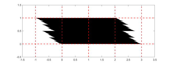
Figure 4.3: The tile generated by the number system of equation (4.12).

The corresponding tile can be seen in Figure 4.3. It turns out that ${\cal F}$ is a tile with tiling set $3\mathbb{Z}\times\mathbb{Z}$ but that tiling set is not equal to $\Delta$. We also point out that a lattice can mean a sublattice of $\mathbb{Z}$ (or $\mathbb{Z}^{m}$). For example, in $\mathbb{R}$,

$$A=3\;,\quad D=\left\{-5,0,20\right\}\,,$$

gives rise to a tile whose tiling set is $\Delta=5\mathbb{Z}$. So the Lebesgue measure of $\cal F$ (a single tile) is 5.

We briefly discuss some general properties of tilings. First, from (3.10) one sees that a tile $\cal F$ satisfies

$${\cal F}=A^{-1}\left({\cal F}+D\right)\,.$$ (4.13)

This leads one to define a map $\tau$ on the space of a priori bounded, compact sets $Z$ (with an appropriate topology), namely

$$\tau(Z)=A^{-1}\left(Z+D\right)\,.$$

One can prove that $\tau$ is a contraction on a complete metric space and thus has a unique fixed point [8]. That fixed point, of course, is $\cal F$ (by (4.13)). The dynamical system $\tau$ is usually called an iterated function system.

On the other hand, (4.13) also — and quite literally — says that $\cal F$ consists of $q$ affine copies ${\cal F}_{i}=A^{-1}({\cal F}+\delta_{i})$ of itself, where $D=\cup_{i=1}^{q}\{\delta_{i}\}$. This allows us to define an expanding map $T$ from $\cal F$ to itself by setting

$$T(x)=Ax-\delta_{i}\;\;\;{\rm if}\;\;\;x\in{\cal F}_{i}\,.$$ (4.14)

This is the generalization of the angle doubling map in equation (1.1). There is a very simple algorithm to generate an expansion for any given vector $x\in\mathbb{R}^{m}$. It is the same algorithm that works in the case that $T(x)=\{2x\}$. Namely, first multiply by $A^{-k}$ (if necessary) to ensure that $x$ is a fractional number, i.e. so that $y=A^{-k}x\in{\cal F}$. Now if $y\in{\cal F}_{i}$, then set $d_{1}:=\delta_{i}$. Then compute $T(y)=Ay-d_{1}$. Next, if $T(y)\in{\cal F}_{j}$, then set $d_{2}:=\delta_{j}$. Compute $T^{2}(y)=AT(y)-d_{2}$, and so on. This computes an expansion of $y$. At the end we multiply back by $A^{k}$ to get the expansion of $x$.

Note that ambiguity arises only in the case where $T^{k}(y)$ falls in the intersection of 2 or more of the ${\cal F}_{i}$.

$$T^{k}(y)=\sum_{i=1}^{\infty}\,A^{-i}d_{i}=\sum_{i=1}^{\infty}\,A^{-i}d_{i}^{\prime}\,.$$

This happens if its image under $AT^{k}(y)$ lies in the intersection of two distinct tiles. In a standard number system, these have measure zero according to Definition 3.1. For each $k$, we obtain a set a measure zero where $d_{k}$ is not unique. Thus the exceptions form a countable union of measure zero sets, and thus have measure zero. In fact, we can do better. For example, if $A:\mathbb{R}^{m}\rightarrow\mathbb{R}^{m}$ is a similarity, the Hausdorff dimension $\partial{\cal F}$ can be computed and is always strictly less than $m$ [15]. The exceptional set, being a countable union of copies, has the same dimension.

5 Tiles and Fluctuations.

In Section 2, we computed the fluctuations for the map given by (1.1). Here we do the same, but now for the more general map defined in (4.14). However, to keep things simple, we consider one example: a 2-dimensional tile with 2 digits. There are exactly 6 possibilities for the characteristic polynomial of $A$, namely [7]: $x^{2}\pm 2$, $x^{2}\pm x+2$, and $x^{2}\pm 2x+2$. Let us consider the last polynomial and set

$$A=\begin{pmatrix}-1&1\\ -1&-1\end{pmatrix}\;,\quad D=\left\{\begin{pmatrix}0\\ 0\end{pmatrix},\begin{pmatrix}1\\ 0\end{pmatrix}\right\}\,.$$ (5.15)

Denote these digits simply by $0$ and $d$. The matrix $A$ has eigenvalues $1\pm i$ and so is a similarity ($\sqrt{2}$ times a rotation by $\frac{-3\pi}{8}$). Therefore the resulting tile $\cal F$ is self-similar as opposed to merely self-affine.

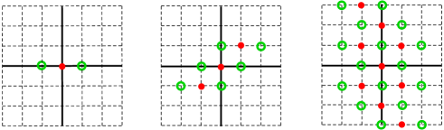
Figure 5.4: Starting from the left with the origin in red. Add the non-zero differences in $D$. In the next figure to the right, in red $A$ times the previous collection of points, then in green the non-zero differences in $D$ are added to each red point.

First, we check that this number system indeed gives the tiling ${\cal F}+\mathbb{Z}^{2}$. By Proposition 4.2, we need to make sure that $\Delta$ equals $\mathbb{Z}^{2}$. The easiest way is to do this recursively as illustrated in Figure 5.4. Start with the origin (left, in red). Then add the non-zero elements of $(D-D)$ (left, in green). Multiply the result by $A$ to get $A(D-D)$ (middle, red) and add $(D-D)$ (middle, green) to get $A(D-D)+(D-D)$. Repeating the procedure to get $A^{2}(D-D)+A(D-D)+(D-D)$ gives the figure on the right. Readers should be able to convince themselves that this recursion obtains $\Delta=\mathbb{Z}^{2}$.

We conclude that ${\cal F}+\mathbb{Z}^{2}$ is a tiling. The corresponding tile can be seen in Figure 5.5. It is known as the Heighway dragon and has a long and storied history (see [13] and references therein).

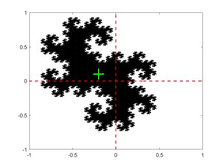
Figure 5.5: The tile generated by the number system of equation (5.15). The center of mass is located at the center of the green cross.

Recall that we are interested in the fluctuations

$$S(n,x)-n\overline{x}=\sum_{i=0}^{n-1}\left\{A^{i}x\right\}\;-n\overline{x}\,,$$

of the map (4.14), where $\overline{x}$ is its average — or center of mass. So we compute the average of $S(n,x)$ with with $x$ uniformly distributed in $\cal F$. Again, Theorem 3.3 gives the answer. For large $n$, the contribution of $\left\{A^{n}x\right\}-x$ is negligible, and so

$$S(n,x)\approx(A-I)^{-1}\sum_{i=1}^{n}d_{i}=p_{n}(A-I)^{-1}d\,,$$ (5.16)

where $p_{n}$ is the number of times $d$ occurs in the first $n$ digits of $x$. The location $\overline{x}$ of the center of mass of this tile follows immediately, since we only have to take the average of $p_{n}$, which is $1/2$. With (5.16) this implies the next result.

Proposition 5.1

The center of mass for the 2-digit tile defined by (5.15), is given by

$$\overline{x}=\frac{1}{2}(A-I)^{-1}d\,.$$

For the Heighway dragon defined by (5.15), we get (see Figure 5.5)

$$\overline{x}:=\frac{1}{2}(A-I)^{-1}d=\frac{1}{10}\begin{pmatrix}-2&-1\\ 1&-2\end{pmatrix}\begin{pmatrix}1\\ 0\end{pmatrix}=\frac{1}{10}\begin{pmatrix}-2\\ 1\end{pmatrix}\,.$$

Together with equation (5.16) this says that $S$ is approximately equal to $2p_{n}\overline{x}$. This implies another, and more remarkable, corollary, namely that, for large $n$, the fluctuations in this 2-digit system lie on the line $t\overline{x}$ where $t\in\mathbb{R}$ ! The limiting distribution itself is easy to figure out since the distribution of $p_{n}$ is exactly the same as the one given in (2.6). This then gives the following proposition.

Proposition 5.2

The distribution of $\;2(S-n\overline{x})\,n^{-1/2}$ tends to the following 1-dimensional distribution as $n\rightarrow\infty$

$$\mathrm{Prob}\left(x\in\left\{t\overline{x}:t\leq\frac{k}{2}\right\}\right)=\frac{1}{\sqrt{2\pi}}\,\int_{-\infty}^{k}\,e^{-\frac{1}{2}u^{2}}\,du\,.$$

To illustrate this counter-intuitive result numerically, we plotted the fluctuations in Figure 5.6 for $n=15$ (left) and $n=50$ (right) together with the line $t\overline{x}$. In each case, we generated $10^{4}$ random binary strings (of length 15 and 50, respectively), computed $S$ for each string, and then plotted $2(S-n\overline{x})n^{-1/2}$. The ‘flattening’ of the distributions is clearly observable.

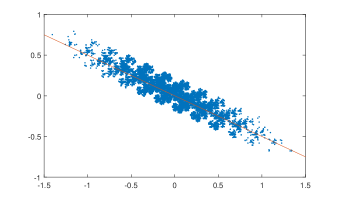
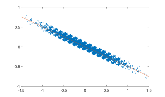
Figure 5.6: The distributions of $\frac{2(S-n\overline{x})}{\sqrt{n}}$ for $n=15$ on the left and for $n=50$ on the right.

Acknowledgment. We are indebted to an anonymous referee for many useful remarks that improved the paper, in particular one observation that ended up strengthening Theorem 3.3.

References

- [1] Arnold, V. I., Avez, A. (1968). Ergodic Problems of Classical Mechanics, New York: Benjamin.
- [2] Banks, J., Brooks, J., Cairns, G., Davis, G., Stacey, P. (1992). On Devaney’s Definition of Chaos. Amer. Math. Monthly. 99(4): 332–334. doi.org/10.2307/2324899
- [3] Bountis, A., Veerman, J. J. P., F. Vivaldi, F. (2020). Cauchy distributions for the integrable standard map. Physics Letters A. 384(26): 126659. doi.org/10.1016/j.physleta.2020.126659
- [4] Conze, J. P., Hervé, L., Raugi, A. (1997). Pavages auto-affines, opérateurs de transfert, et critères de réseau dans . Bol. Soc. Bras. Mat. 28: 1–42. doi.org/10.1007/BF01235987
- [5] Devaney, R. L. (2003). An Introduction to Chaotic Dynamical Systems, 2nd ed. Boca Raton, FL: CRC Press.
- [6] Gröchenig, K. (1994). Orthogonality criteria for compactly supported scaling functions. Appl. Comput. Harmon. Anal. 1(3): 242–245. doi.org/10.1006/acha.1994.1011
- [7] Hacon, D., Saldanha, N. C., Veerman, J. J. P. (1994). Remarks on self-affine tilings. Exp. Math. 3(4): 317–327. doi.org/10.1080/10586458.1994.10504300
- [8] Hutchinson, J. E. (1981). Fractals and self-similarity. Indiana Univ. Math. J. 30(5): 713–747.
- [9] Kac, M. (1959). Statistical Independence in Probability, Analysis and Number Theory. The Carus Mathematical Monographs, Vol. 12. Washington, DC: The Mathematical Association of America.
- [10] Lagarias, J. C., Wang, Y. (1996). Self-affine tiles in . Advances in Mathematics. 121(1): 21–49. doi.org/10.1006/aima.1996.0045
- [11] Lagarias, J. C., Wang, Y. (1997). Integral self-affine tilings in II: Lattice tilings. J. Fourier Anal. Appl. 3(1): 83–102. doi.org/10.1007/BF02647948
- [12] Reichl, L. (2016). A Modern Course in Statistical Physics, 4th ed. New York: Wiley.
- [13] Tabachnikov, S. (2014). Dragon curves revisited. The Mathematical Intelligencer. 36(1): 13–17. doi.org/10.1007/s00283-013-9428-y
- [14] Tsallis, C. (2009). Introduction to Nonextensive Statistical Mechanics. New York: Springer-Verlag.
- [15] Veerman, J. J. P. (1998). Hausdorff dimension of boundaries of self-affine tiles in . Bol. Soc. Mat. Mex. 4(2): 159–182.
- [16] Veerman, J. J. P., Oberly, P. J., Fox, L. S. (2021). Statistics of a family of piecewise linear maps. Phys. D. 427: 133019. doi.org/10.1016/j.physd.2021.133019