Causal Inference with Truncation-by-Death and Unmeasured Confounding

Abstract

Clinical studies sometimes encounter truncation by death, rendering outcomes undefined. Statistical analysis based solely on observed survivors may give biased results because the characteristics of survivors differ between treatment groups. By principal stratification, the survivor average causal effect was proposed as a causal estimand defined in always-survivors. However, this estimand is not identifiable when there is unmeasured confounding between the treatment assignment and survival or outcome process. In this paper, we consider the comparison between an aggressive treatment and a conservative treatment with monotonicity on survival. First, we show that the survivor average causal effect on the conservative treatment is identifiable based on a substitutional variable under appropriate assumptions, even when the treatment assignment is not ignorable. Next, we propose an augmented inverse probability weighting (AIPW) type estimator for this estimand with double robustness. Finally, large sample properties of this estimator are established. The proposed method is applied to investigate the effect of allogeneic stem cell transplantation types on leukemia relapse.

Keywords: Ignorability; Observational study; Principal stratification; Substitutional variable; Survivor average causal effect.

1 Introduction

In clinical studies with mortality, outcomes other than mortality (such as quality of life following surgery) may be of primary interest. Since some individuals die before their primary outcomes are evaluated, we cannot measure those outcomes. This phenomenon is known as the truncation-by-death problem (Rubin, , 2000; McConnell et al., , 2008). Truncation-by-death is a different concept from censoring in that the latter indicates that an outcome exists but is not recorded, resulting in missing data, whereas the former renders the outcomes undefined. Because the observed survivors may consist of units with possibly different unmeasured characteristics, the observed outcomes in survivors between different treatment groups are not comparable.

A proper way to handle the truncation-by-death problem is principal stratification (Frangakis and Rubin, , 2002; Rubin, , 2006). Principal strata are typically defined by the joint potential values of a post-treatment intermediate variable (Jiang and Ding, , 2021). Because the potential values of the intermediate variable for a unit are irrelevant to the treatment that the unit actually received, the principal stratum reflects the unit’s intrinsic characteristics and acts as a baseline covariate. A meaningful causal contrast can only be defined in a subpopulation whose both potential outcomes are well defined, and such an estimand is often referred to as the survivor average causal effect (SACE). However, since the always-survivors are not individually observable, the interpretation of SACE should be paid extraordinary caution.

To study the SACE, Zhang and Rubin, (2003), Imai, (2008), Chiba and VanderWeele, (2011), Chiba, (2011), and Long and Hudgens, (2013) provided bounds for this estimand. Yang and Small, (2016) also used post-treatment information to construct bounds. However, these bounds are often too wide and not very useful for statistical inference. To point-identify the SACE, a commonly adopted assumption is the monotonicity of survival with respect to treatment. In addition to monotonicity, the relationship between the survival and outcome is sometimes assumed to follow a biased selection model or pattern mixture model with hyperparameters (Gilbert et al., , 2003; Shepherd et al., , 2006; Jemiai et al., , 2007). In some studies, the biased selection model has been replaced with an independence assumption between the principal strata and potential outcomes in observed survivors, which is referred to as explainable nonrandom survival or principal ignorability (Hayden et al., , 2005; Egleston et al., , 2007; Ding and Lu, , 2017). Sensitivity analysis can be performed to assess the feasibility of the biased selection model or independence assumption.

If various types of covariates are available, information regarding survival can be leveraged to point-identify the SACE, which calls for a covariate playing a functioning role. Conditional independence is constructed using this key covariate. Ding et al., (2011) considered the identification of the SACE based on a baseline covariate whose distribution is informative of the principal strata in randomized experiments, but assumed no common causes for the survival and outcome processes. A simulation study conducted by McGuinness et al., (2019) indicated that unmeasured survival–outcome confounding would bias the estimation of the SACE. Tchetgen Tchetgen, (2014) used post-treatment correlates of survival and outcomes in longitudinal studies to identify the SACE under nonparametric structural equations models. Further, Wang et al., (2017) used a substitutional variable correlated with principal strata in addition to a variety of covariates to identify the SACE.

However, most methods for handling the truncation-by-death problem assumed no unmeasured confounding between the treatment assignment and survival process. These methods rely on ignorability so that the proportions of principal strata in both treatment groups are identical. Theoretically, statistical analysis becomes more challenging without ignorability because we would have no information about the distribution of principal strata. There are two possible ways to acheive identifiability in the presence of unmeasured confounding. The first is to restrict the relationship between the survival (principal strata) and outcome process (potential outcomes), such as introducing the explainable nonrandom survival assumption (Egleston et al., , 2009), which omits the influence of principal strata on potential outcomes. The second way is to explore the unmeasured confoundedness between the treatment assignment and survival process by introducing a latent variable (Kédagni, , 2021). However, this approach cannot identify the SACE because the proportions of principal strata are inestimable, unless there is more information about the outcome distribution in different principal strata.

In this paper, we consider observational studies with unmeasured confounding when some outcomes are truncated by death. The unmeasured confounding matters in the following two aspects. On the one hand, the unmeasured confounding between the treatment–survival processes renders the distributions of principal strata different between treatment groups. The target population is hard to define and identify because the always-survivors in different treatment groups are different in unmeasured features. On the other hand, the unmeasured confounding between the survival–outcome processes results in a cross-world reliance of potential outcomes on potential survivals. The causal effect in always-survivors is hard to identify because the observed outcomes are mixed from more than one principal stratum. This setup is referred to as latent ignorability, where the principal strata (joint potential survivals) confound the treatment–survival–outcome processes simultaneously.

The innovation is twofold. First, we contribute to causal inference with unmeasured confounding by proposing a substitutional variable strategy. The substitutional variable is a baseline proxy of the always-survivorship (latent indicator of the target population) which do not require the equivalence or completeness assumption as required in auxiliary approaches or negative controls (Tchetgen Tchetgen et al., , 2020; Miao et al., , 2022). We show that the survivor average causal effect on the conservative treatment group (SACEC) can be identified with a single substitutional variable under certain assumptions, even though the SACE in the overall population is not identifiable. The core assumption on the substitutional variable can be assessed by sensitivity analysis. Second, an augmented inverse probability weighting (AIPW) type estimator is proposed to estimate the SACEC with double robustness. Large sample properties of this AIPW type estimator are established.

The remainder of this paper is organized as follows. In Section 2, we introduce the motivating data, notations and causal estimands under the potential outcome framework. In Section 3, we present assumptions for identifying causal effects. Estimation and a sensitivity analysis framework are also illustrated in this section. Simulation studies are presented in Section 4 to compare the proposed method to existing methods. The proposed method is applied to a retrospective allogeneic stem cell transplantation dataset to investigate the effects of transplantation types on leukemia relapse in Section 5. This paper concludes with a brief summary of our findings. The supporting information includes causal graphs, proofs of theorems and additional simulation results.

2 Motiviting data and causal estimands

2.1 Motivating data

Allogeneic stem cell transplantation is a widely adopted approach to treat acute lymphoblastic leukemia, including human leukocyte antigen (HLA)-matched sibling donor transplantation (MSDT) and haploidentical stem cell transplantation (haplo-SCT) from family. The non-relapse mortality (NRM) for MSDT is lower than that for haplo-SCT becasue there are fewer mismatched HLA loci between the donor and patient undergoing MSDT, so doctors usually prefer MSDT. In recent years, some benefits of haplo-SCT have been noted, in that stronger graft-versus-leukemia effects with haplo-SCT are found (Chang et al., , 2017, 2020).

It is important to know whether haplo-SCT can achieve competitive performances with MSDT in terms of relapse if patients can survive, as the maturing operations are leading to higher survival rate. Formally speaking, we are interested in the treatment effect of transplantation types on relapse in always-survivors undergoing haplo-SCT. Statistical findings based on causal inference would help establish clinical guidelines for allogeneic stem cell transplantation.

Data from a retrospective study were collected at Peking University People’s Hospital in China, including 1161 patients undergoing allogeneic stem cell transplantation from 2009 to 2017 (Ma et al., , 2021). In the dataset, 21.53% patients received MSDT (with no mismatched HLA loci) and 78.47% received haplo-SCT (with mismatched HLA loci). By the end of two years after transplantation, the survival rate is 89.60% for MSDT and 84.96% for haplo-SCT. Among survivors, the relapse rate is 21.88% for MSDT and 18.99% for haplo-SCT.

2.2 Estimands

Consider an observational study with binary treatments such that $Z=1$ for the aggressive treatment (MSDT) and $Z=0$ for the conservative treatment (haplo-SCT). Let $S(z)$ be the binary potential survival ($z=0,1$), where $S(z)=1$ if the subject would survive and $S(z)=0$ otherwise. A potential outcome (incidence of relapse) $Y(z)$ is defined only if $S(z)=1$. We can supplementarily denote $Y(z)=*$ if $S(z)=0$. We assume a stable unit treatment value and consistency. Then $S=ZS(1)+(1-Z)S(0)$ and $Y=ZY(1)+(1-Z)Y(0)$ whenever an outcome is well defined. Baseline covariates $(V,X)$ on supports $\mathcal{V}\times\mathcal{X}$ are collected. Here $X$ act as measured confounders and $V$ acts as a substitutional variable for $S(0)$; a rigourous statement is deferred to next section. Let the subscript $i=1,\ldots,n$ denote the indexes of subjects. The observed sample $\{O_{i}=(Z_{i},S_{i},Y_{i},X_{i},V_{i}):i=1,\ldots,n\}$ is independently drawn from an infinite super-population.

Stratified by the joint values of $G=(S(1),S(0))$, there are four principal strata (Ding et al., , 2011): LL (always-survivors), LD (protected), DL (harmed), and DD (doomed); see Table 1. Often the DL stratum is excluded by a monotonicity assumption. The observed survivors in the aggressive treatment group come from the LL and LD strata, whereas the survivors in the conservative treatment group come from the LL stratum.

Table 1: Principal strata (✓means well defined and $*$ means undefined)

Stratum	$S(1)$	$S(0)$	$Y(1)$	$Y(0)$	Description
LL	1	1	✓	✓	Always-survivors
LD	1	0	✓	$*$	Protected
DL	0	1	$*$	✓	Harmed	(Excluded by monotonicity)
DD	0	0	$*$	$*$	Doomed

To define a meaningful causal estimand, we should restrict our analysis on the LL stratum, where both potential outcomes are well defined. The survivor average causal effect on the overall population (SACE), on the aggressive treatment (SACET) and on the conservative treatment (SACEC) are defiend as

$$\Delta=E\{Y(1)-Y(0)\mid G=\text{LL}\},\ \Delta_{\operatorname{T}}=E\{Y(1)-Y(0)\mid G=\text{LL},Z=1\},$$

$$\Delta_{\operatorname{C}}=E\{Y(1)-Y(0)\mid G=\text{LL},Z=0\},$$

respectively. These three estimands generally are not equal because $Z$ is confounded with $G$. In some circumstances, the aggressive treatment may induce unsatisfactory quality of life despite survival. Practitioners would like to know whether the conservative treatment is sufficient for survivable patients, so they care about $\Delta_{\operatorname{C}}$. Another advantage of adopting $\Delta_{\operatorname{C}}$ as the estimand is that its target population is individually observed as the survivors receiving the conservative treatment.

3 Identification and Estimation

3.1 Identification of the causal estimand using a substitutional variable

Suppose there is an unmeasured confounder $U$ between the treatment $Z$ and principal stratum $G$ (Kédagni, , 2021). The backdoor paths from $Z$ to $(Y(1),Y(0))$ are blocked by $(V,X)$ and $G$. So we assume latent ignorability as follows, which is weaker than and can be implied by ignorability.

Assumption 1 (Latent ignorability)

$Y(z)\mathchoice{\mathrel{\hbox to0.0pt{$\displaystyle\perp$\hss}\mkern 2.0mu{\displaystyle\perp}}}{\mathrel{\hbox to0.0pt{$\textstyle\perp$\hss}\mkern 2.0mu{\textstyle\perp}}}{\mathrel{\hbox to0.0pt{$\scriptstyle\perp$\hss}\mkern 2.0mu{\scriptstyle\perp}}}{\mathrel{\hbox to0.0pt{$\scriptscriptstyle\perp$\hss}\mkern 2.0mu{\scriptscriptstyle\perp}}}Z\mid G=\text{LL},V,X$ for $z=0,1$.

By controlling as many predictors of $Z$ and risk factors of $Y$ as possible, latent ignorability can be plausible.

Assumption 2 (Monotonicity)

$S(1)\geq S(0)$ almost surely.

Assumption 3 (Positivity)

$0<\operatorname{pr}(Z=1\mid V,X)<1$, $0<\operatorname{pr}(S(0)=1\mid Z=1,V,X)<1$, and $\operatorname{pr}(S(0)=1\mid Z=0,V,X)>0$.

Monotonicity is often reasonable in observational studies. The aggressive treatment should produce a higher survival rate than the conservative treatment in a short period. Positivity and monotonicity ensure that always-survivors and doomed individuals exist in the aggressive treatment group. To disentangle the mixture of LL and LD in this aggressive treatment group, a substitutional variable for $S(0)$ is needed.

Assumption 4 (Substitution relevance)

$V\not\mathchoice{\mathrel{\hbox to0.0pt{$\displaystyle\perp$\hss}\mkern 2.0mu{\displaystyle\perp}}}{\mathrel{\hbox to0.0pt{$\textstyle\perp$\hss}\mkern 2.0mu{\textstyle\perp}}}{\mathrel{\hbox to0.0pt{$\scriptstyle\perp$\hss}\mkern 2.0mu{\scriptstyle\perp}}}{\mathrel{\hbox to0.0pt{$\scriptscriptstyle\perp$\hss}\mkern 2.0mu{\scriptscriptstyle\perp}}}S(0)\mid Z=1,S(1)=1,X$.

Assumption 5 (Nondifferential substitution)

$V\mathchoice{\mathrel{\hbox to0.0pt{$\displaystyle\perp$\hss}\mkern 2.0mu{\displaystyle\perp}}}{\mathrel{\hbox to0.0pt{$\textstyle\perp$\hss}\mkern 2.0mu{\textstyle\perp}}}{\mathrel{\hbox to0.0pt{$\scriptstyle\perp$\hss}\mkern 2.0mu{\scriptstyle\perp}}}{\mathrel{\hbox to0.0pt{$\scriptscriptstyle\perp$\hss}\mkern 2.0mu{\scriptscriptstyle\perp}}}S(1)\mid Z=1,S(0)=0,X$.

Assumption 6 (Non-interaction)

$E\{Y(z)\mid G,V,X\}=E\{Y(z)\mid G,X\}+f(V,X)$ for some maybe unknown function $f(V,X)$.

Substitution relevance helps distinguish LL and LD strata among observed survivors using the substitutional variable. Nondifferential substitution states that $V$ is a baseline proxy of $S(0)$, whose measurement error is irrelevant to $S(1)$. The substitutional variable can also be understood as a proxy of the always-survivorship in the $Z=1$ group, which contains information of the indicator of target population but does not contain irrelevant information. Nondifferential substitution can be implied by the combination of $V\mathchoice{\mathrel{\hbox to0.0pt{$\displaystyle\perp$\hss}\mkern 2.0mu{\displaystyle\perp}}}{\mathrel{\hbox to0.0pt{$\textstyle\perp$\hss}\mkern 2.0mu{\textstyle\perp}}}{\mathrel{\hbox to0.0pt{$\scriptstyle\perp$\hss}\mkern 2.0mu{\scriptstyle\perp}}}{\mathrel{\hbox to0.0pt{$\scriptscriptstyle\perp$\hss}\mkern 2.0mu{\scriptscriptstyle\perp}}}S(1)\mid S(0)=0,X$ and $S(1)\mathchoice{\mathrel{\hbox to0.0pt{$\displaystyle\perp$\hss}\mkern 2.0mu{\displaystyle\perp}}}{\mathrel{\hbox to0.0pt{$\textstyle\perp$\hss}\mkern 2.0mu{\textstyle\perp}}}{\mathrel{\hbox to0.0pt{$\scriptstyle\perp$\hss}\mkern 2.0mu{\scriptstyle\perp}}}{\mathrel{\hbox to0.0pt{$\scriptscriptstyle\perp$\hss}\mkern 2.0mu{\scriptscriptstyle\perp}}}Z\mid S(0)=0,V,X$. Non-interaction means that the effect of $V$ on $Y$ does not modify the effects of $G$ or $Z$ on $Y$. A special case of non-interaction is exclusion restriction, where $V$ does not have direct effect on $(Y(1),Y(0))$ so that $f(v,x)\equiv 0$.

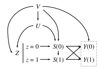
Figure 1: A causal structural model. Baseline covariates $X$, which can have edges to $V$, $Z$, $U$, $S(0)$, $S(1)$, $Y(0)$ and $Y(1)$, are omitted for simplicity.

Figure 1 presents a possible causal structural model with an unmeasured confounder $U$ between $Z$ and $G=(S(1),S(0))$. Potential outcomes $(Y(1),Y(0))$ can depend on $G$. The substitutional variable has association with $S(0)$, but its association with $S(1)$ is blocked by $S(0)$ as a result of substitution relevance and nondifferential substitution. In Supplementary Material A, we give some examples that satisfy these six assumptions.

Define the propensity score, survival score and outcome regression model as

$$e(v,x) =\operatorname{pr}(Z=1\mid V=v,X=x),$$

$$\pi_{z}(v,x) =\operatorname{pr}(S=1\mid Z=z,V=v,X=x),$$

$$m_{z}(v,x) =E(Y\mid Z=z,S=1,V=v,X=x),$$

respectively, for $z=0,1$. We denote the proportions of principal strata in the aggressive treatment group as $\pi_{g}(v,x)=\operatorname{pr}(G=g\mid Z=1,V=v,X=x)$ for $g\in\{\text{LL},\text{LD},\text{DD}\}$.

Denote $E_{V|X}\{g(V,X)\}=E\{g(V,X)\mid X\}$ for any measurable function $g(V,X)$ with finite expectation. Let $h(v,x)$ be an integrable function with respect to $v$ subject to

$$E_{V|X}\left\{h(V,X)\right\}=0,\quad E_{V|X}\left\{\frac{\pi_{\text{LL}}(V,X)}{\pi_{\text{LD}}(V,X)}h(V,X)\right\}\neq 0.$$

Define weight functions

$$R(v,x) =\frac{\frac{\pi_{1}(v,x)}{1-\pi_{1}(v,x)}h(v,x)}{E_{V|X=x}\left\{\frac{\pi_{1}(V,X)}{1-\pi_{1}(V,X)}h(V,X)\right\}},$$

$$R_{0}(v,x) =\frac{(1-e(v,x))\pi_{0}(v,x)}{\operatorname{pr}(Z=0,S=1)},\quad R_{1}(v,x)=R(v,x)E_{V|X=x}\{R_{0}(V,X)\}.$$

The function $R_{0}(v,x)$ represents a covariate shift from the overall population to the survivors (always-survivors) in the conservative treatment group ($Z=0$). We have the following identification result.

Theorem 1

Under Assumptions 1–6, SACEC can be identified,

$$\Delta_{\operatorname{C}} =E\left[R_{1}(V,X)\{m_{1}(V,X)-m_{0}(V,X)\}\right]$$ (1)

$$=E\left[R_{1}(V,X)\left\{\frac{ZS(Y-m_{1}(V,X))}{e(V,X)\pi_{1}(V,X)}+m_{1}(V,X)-m_{0}(V,X)\right\}\right.$$

$$\qquad\qquad\qquad\left.-R_{0}(V,X)\left\{\frac{(1-Z)S(Y-m_{0}(V,X))}{(1-e(V,X))\pi_{0}(V,X)}\right\}\right].$$ (2)

Remark 1

If $V$ is not binary, then there are many possible ways to construct $h(v,x)$ since only two values of $V$ are required for identification. Different choices of $h(v,x)$ can lead to a unique solution of $\Delta_{\operatorname{C}}$. For example, we can take $h(v,x)=v-E(V|X=x)$.

The proof of Theorem 1 is given in Supplementary Material B. The proportion of always-survivors in the $Z=1$ group is not identifiable under Assumptions 1–6, so SACE and SACET are not identifiable.

Now we give three examples to illustrate when this identification strategy based on the substitutional variable can be reasonable.

Example 1. Suppose a traditional therapy (such as chemotherapy) has been widely adopted to cure a disease, but this therapy may cause adverse effects (readmission). Now a novel therapy (such as medication) is invented, which can greatly lower the safety risk, so monotonicity holds. In a cohort study, patients decided proper treatments to take based on doctor’s suggestion. Let $Z$ be the treatment a patient received, $S$ be the occurence of readmission, and $Y$ be the outcome of interest, such as quality of life. We want to measure the treatment effect on quality of life at home. The substitutional variable $V$ can be a baseline risk factor of the adverse effect for the chemotherapy. By definition, $V$ satisfies substitution relevance and nondifferential substitution since $V$ is irrelevant to medication outcomes. Suppose the risk factor $V$ would not affect the quality of life if this patient can live normally outside the hospital, so exclusion restriction (non-interaction) is also satisfied.

Example 2. Suppose a targeted durg is used to cure cancer. This targeted drug is effective only if the patient carry certain gene. Now a generic drug targeting on a wider range of but unconfirmed population is invented. Let $Z$ indicate which drug to take, $S$ be an indicator indicating whether a patient response to the drug, and $Y$ be the outcome of interest. Practitioners want to know whether the generic drug has a better performance than the targeted drug. To make these two drugs comparative, the study should condition on the subpopulation who are responsive to both drugs. In a clinical trial, patients with PCR testing positive for the targeted gene are randomized to take the targeted drug or generic drug, while patients with PCR testing negative are all assigned to take the generic drug. Monotonicity means that the patients with PCR testing positive are also eligible for the generic drug, ensured by the wider target of the generic drug. The substitutional variable $V$ can be the PCR test result. It satisfies substitution relevance and nondifferential substitution because the PCR test cannot predict the response to the generic drug if a patient does not respond to the targeted drug. It also satisfies non-interaction because PCR test results cannot directly influence outcomes: it is $G=(S(1),S(0))$ that may influence outcomes.

Example 3. Suppose the government puts forward a training program to promote employment for job finders. Here $Z$ is whether a person joins in the program, $S$ is an indicator of employment, and $Y$ is the earning if employed. The government wants to know the effect of this program on earnings, so the study should restrict to the always-employed subpopulation. A person who tends to be unemployed would be more willing to join in the program. Monotonicity means that joining in the program would make job finding easier. The substitutional variable $V$ can be self-reported confidence of successfully finding a job before joining in the program, so $V$ satisfies substitution relevance and nondifferential substitution. Such a variable $V$ can be collected by questionnaire when signing up for the program. Non-interaction is also reasonable because once he/she is employed, the pre-treatment confidence for being employed measured before joining in the training program would not make a difference on earnings whether he/she joined in the training program or not.

3.2 Estimation of the causal effect

Suppose $e(v,x)$, $\pi_{z}(v,x)$, $m_{z}(v,x)$ and $R_{z}(v,x)$ are estimated as $\widehat{e}(v,x)$, $\widehat{\pi}_{z}(v,x)$, $\widehat{m}_{z}(v,x)$ and $\widehat{R}_{z}(v,x)$, respectively for $z=0,1$. The denominator of $R(v,x)$ can be estimated by empirical average in a neighborhood of each $(v,x)$ based on the Mahalanobis distance or kernel.

We focus on the property of the model-assisted AIPW type estimator

$$\widehat{\Delta}_{\operatorname{C}} =\mathbb{E}_{n}\left[\widehat{R}_{1}(V,X)\left\{\frac{ZS(Y-\widehat{m}_{1}(V,X))}{\widehat{e}(V,X)\widehat{\pi}_{1}(V,X)}+\widehat{m}_{1}(V,X)-\widehat{m}_{0}(V,X)\right\}\right.$$

$$\qquad\qquad\qquad\left.-\widehat{R}_{0}(V,X)\left\{\frac{(1-Z)S(Y-\widehat{m}_{0}(V,X))}{(1-\widehat{e}(V,X))\widehat{\pi}_{0}(V,X)}\right\}\right],$$ (3)

where $\mathbb{E}_{n}(\cdot)$ means empirical average on the full sample. Let $\widehat{\Delta}_{\operatorname{C}}^{*}$ be the oracle estimator in which all models are known,

$$\widehat{\Delta}_{\operatorname{C}}^{*}=\mathbb{E}_{n}\{\phi(O)\} =\mathbb{E}_{n}\left[R_{1}(V,X)\left\{\frac{ZS(Y-m_{1}(V,X))}{e(V,X)\pi_{1}(V,X)}+m_{1}(V,X)-m_{0}(V,X)\right\}\right.$$

$$\qquad\qquad\qquad\left.-R_{0}(V,X)\left\{\frac{(1-Z)S(Y-m_{0}(V,X))}{(1-e(V,X))\pi_{0}(V,X)}\right\}\right].$$ (4)

The oracle estimator $\widehat{\Delta}_{\operatorname{C}}^{*}$ enjoys asymptotic normality $n^{1/2}(\widehat{\Delta}_{\operatorname{C}}^{*}-\Delta_{\operatorname{C}})\rightarrow_{d}N(0,C)$, where

$$C=E\left\{\frac{R_{1}(V,X)^{2}\operatorname{var}(Y|V,X,Z=1)^{2}}{e(V,X)\pi_{1}(V,X)}+\frac{R_{0}(V,X)^{2}\operatorname{var}(Y|V,X,Z=0)^{2}}{(1-e(V,X))\pi_{0}(V,X)}\right\}+\operatorname{var}\{\Delta(X)\}.$$

There is higher-order bias between $\widehat{\Delta}_{\operatorname{C}}$ and $\widehat{\Delta}_{\operatorname{C}}^{*}$ due to the variation of estimated models. By cross-fitting (Chernozhukov et al., , 2018), the discrepency can be described by a drift term converging to zero in probability under correct model specifications,

$$D_{n} =\mathbb{E}_{n}\Big{\{}(\widehat{R}_{1}(V,X)-R_{1}(V,X))(m_{1}(V,X)-m_{0}(V,X))$$

$$\qquad\qquad\qquad-(R_{1}(V,X)-R_{0}(V,X))(\widehat{m}_{0}(V,X)-m_{0}(V,X))\Big{\}}.$$

The large sample properties of $\widehat{\Delta}_{\operatorname{C}}$ is demonstrated in the following theorem.

Theorem 2

(a) If $\{\widehat{m}_{0}(v,x),\widehat{R}_{z}(v,x):z=0,1\}$ are sup-norm consistent upon $(v,x)\in\mathcal{V}\times\mathcal{X}$, then $\widehat{\Delta}_{\operatorname{C}}^{*}$ and $\widehat{\Delta}_{\operatorname{C}}$ converge in probability to $\Delta_{\operatorname{C}}$ if either $\{\widehat{e}(v,x),\widehat{\pi}_{z}(v,x):z=0,1\}$ or $\widehat{m}_{1}(v,x)$ is sup-norm consistent upon $(v,x)\in\mathcal{V}\times\mathcal{X}$.
(b) If $\{\widehat{e}(v,x),\widehat{\pi}_{z}(v,x),\widehat{m}_{z}(v,x),\widehat{R}_{z}(v,x):z=0,1\}$ are sup-norm consistent upon $(v,x)\in\mathcal{V}\times\mathcal{X}$, and converge at rates faster than $o_{p}(n^{-1/4})$, then $n^{1/2}(\widehat{\Delta}_{\operatorname{C}}-\widehat{\Delta}_{\operatorname{C}}^{*}-D_{n})\rightarrow_{p}0$.
(c) Further in (b), if the estimators of the parameters in $R_{1}(v,x;\theta_{1})$ and $m_{0}(v,x;\theta_{0})$ are regular and asymptotic linear (RAL) with influence functions $\psi_{1}(O)$ and $\psi_{0}(O)$, then $\widehat{\Delta}_{\operatorname{C}}$ is regular and asymptotic linear with influence function $\psi(O)=\phi(O)-\Delta_{\operatorname{C}}+\Gamma_{1}\psi_{1}(O)-\Gamma_{0}\psi_{0}(O)$ under some regularity conditions, where

$$\Gamma_{1} =E\left[\frac{\partial R_{1}(V,X;\theta_{1})}{\partial\theta_{1}}\{m_{1}(V,X)-m_{0}(V,X)\}\right],$$

$$\Gamma_{0} =E\left[\frac{\partial m_{0}(V,X;\theta_{0})}{\partial\theta_{0}}\{R_{1}(V,X)-R_{0}(V,X)\}\right].$$

Thus, $n^{1/2}(\widehat{\Delta}_{\operatorname{C}}-\Delta_{\operatorname{C}})\rightarrow_{d}N(0,E\{\psi(O)^{2}\})$.

Part (a) of Theorem 2 indicates the double robustness of the AIPW type estimator. In practice, the observed survivors in the aggressive treatment group come from two principal strata, so $m_{1}(v,x)$ is likely to be misspecified. Double robustness provides insurance to model misspecification. Part (b) shows the higher-order bias of $\widehat{\Delta}_{\operatorname{C}}$ from the oracle estimator $\widehat{\Delta}_{\operatorname{C}}^{*}$. Part (c) establishes the asymptotic distribution. The proof of Theorem 2 is given in Supplementary Material C.

3.3 Sensitivity analysis for nondifferential substitution

To relax the nondifferential substitution, additional knowledge regarding the behaviors of $V$ in the LD and DD strata is required. For an arbitrary $v_{0}\in\mathcal{V}$, let

$$\rho(v,x)=\frac{\pi_{\text{DD}}(v,x)}{\pi_{\text{LD}}(v,x)}\Big{/}\frac{\pi_{\text{DD}}(v_{0},x)}{\pi_{\text{LD}}(v_{0},x)},$$

which measures the odds ratio of DD over LD in the aggressive treatment group. Nondifferential substitution (Assumption 5) implies that $\rho(v,x)\equiv 1$. Let

$$R^{*}(v,x)=\frac{\frac{\pi_{1}(v,x)}{1-\pi_{1}(v,x)}\rho(v,x)h(v,x)}{E_{V|X=x}\left\{\frac{\pi_{1}(V,X)}{1-\pi_{1}(V,X)}\rho(V,X)h(V,X)\right\}}.$$

Without nondifferential substitution, if $\rho(v,x)$ is known, then SACEC can be identified by replacing $R(v,x)$ with $R^{*}(v,x)$ in Equations (1) and (2).

Remark 2

If weak $S$-ignorability $S(0)\mathchoice{\mathrel{\hbox to0.0pt{$\displaystyle\perp$\hss}\mkern 2.0mu{\displaystyle\perp}}}{\mathrel{\hbox to0.0pt{$\textstyle\perp$\hss}\mkern 2.0mu{\textstyle\perp}}}{\mathrel{\hbox to0.0pt{$\scriptstyle\perp$\hss}\mkern 2.0mu{\scriptstyle\perp}}}{\mathrel{\hbox to0.0pt{$\scriptscriptstyle\perp$\hss}\mkern 2.0mu{\scriptscriptstyle\perp}}}Z\mid V,X$ holds, then $\pi_{\text{DD}}(v,x)=1-\pi_{1}(v,x)$ and $\pi_{\text{LD}}(v,x)=\pi_{1}(v,x)-\pi_{0}(v,x)$. The nondifferential substitution assumption on the substitutional variable can be relaxed, in that $V$ can contain information of both $S(0)$ and $S(1)$. Without nondifferential substitution, taking a $v_{0}\in\mathcal{V}$, $\rho(v,x)$ is identified as

$$\rho(v,x)=\frac{1-\pi_{1}(v,x)}{\pi_{1}(v,x)-\pi_{0}(v,x)}\Big{/}\frac{1-\pi_{1}(v_{0},x)}{\pi_{1}(v_{0},x)-\pi_{0}(v_{0},x)}.$$

Remark 3

Although the substitutional variable $V$ plays an important role in identifying the causal estimand, interestingly, invoking the substitutional variable does not help identify $\Delta_{\operatorname{C}}$ under explainable nonrandom survival (also known as principal ignorability; Hayden et al., , 2005; Ding and Lu, , 2017): $E\{Y(1)\mid G=\text{LL},V,X\}=E\{Y(1)\mid G=\text{LD},V,X\}.$ The estimation of SACEC can be consistent for any misspecified $\rho(v,x)$; see Supplementary Material B. So a hypothesis test can be performed,

$$H_{0}:m_{1}(v_{1},x)-m_{0}(v_{1},x)=m_{1}(v_{2},x)-m_{0}(v_{2},x)~{}\mbox{ for any }v_{1},v_{2}\in\mathcal{V}.$$

If the null hypothesis $H_{0}$ is not rejected, then the naive (survivor-case) estimator based solely on observed surivors would not suffer from severe bias.

Typically, $\rho(v,x)$ is not identifiable from observed data, which motivates a sensitivity analysis to assess the influence of $\rho(v,x)$ on the estimator. Suppose $\pi_{1}(v,x)$ is estimated by logistic regression, $\pi_{1}(v,x)/\{1-\pi_{1}(v,x)\}=\exp(\beta_{c}+x\beta_{x}+v\beta_{v})$, and $\rho(v,x)$ is chosen as $\rho(v,x)=\exp(\eta_{c}+x\eta_{x}+v\eta_{v})$, then

$$R^{*}(v,x)=\frac{\exp\{v(\beta_{v}+\eta_{v})\}h(v,x)}{\int_{\mathcal{V}}\exp\{v(\beta_{v}+\eta_{v})\}h(v,x)p(v|x)dv}.$$

We can introduce a sensitivity parameter $\eta\in(-1,1)$ and let $\eta_{v}=-\widehat{\beta}_{v}\log_{2}(1-\eta)$. Without loss of generality, suppose $\widehat{\beta}_{v}>0$, so $\eta_{v}\in(-\widehat{\beta}_{v},\infty)$. Here we do not allow $\eta_{v}$ to move lower than $-\widehat{\beta}_{v}$ because we want to maintain substitution relevance.

Alternatively, we can determine the value of $\rho(v,x)$ using external interventional data; see Supplementary Material D. This setting is reasonable for post-marketing safety or effectiveness assessment based on observational data after a drug has proven beneficial for survival in some previous randomized trials.

4 Simulation studies

In this section, we compare our proposed method with the naive survivor-case analysis and the method of Wang et al., (2017) which requires $S$-ignorability. We generate covariates $X$ independently from

$$\left(\begin{array}[]{c}X_{1}\\ X_{2}\end{array}\right)\sim N\left(\left(\begin{array}[]{c}1\\ 1\end{array}\right),~{}\left(\begin{array}[]{cc}1^{2}&~{}0.5\\ 0.5&~{}1^{2}\end{array}\right)\right),\quad X_{3}\sim U(0,2),$$

where $N(\mu,\sigma^{2})$ denotes a normal distribution with mean $\mu$ and variance $\sigma^{2}$, and $U(l,u)$ denotes a uniform distribution on $(l,u)$. Write $X=(1,X_{1},X_{2},X_{3})$. The substitutional variable is generated from $V\sim N(X\zeta,2^{2})$. The individualized treatment is assigned according to $\operatorname{pr}(Z=1\mid V,X)=\operatorname{expit}\{(X,V)\alpha\}$, where $\operatorname{expit}(x)=\exp(x)/\{1+\exp(x)\}$.

Since there may be unmeasured confounding between $Z$ and $S$, we generate the potential survivals separately in the aggressive and conservative treatment groups:

$$\operatorname{pr}(S(0)=1\mid V,X,Z=z)=\operatorname{expit}\{(X,V)\beta_{z}\},$$

$$\operatorname{pr}(S(1)=1\mid V,X,Z=z,S(0)=0)=\operatorname{expit}\{(X,V)\gamma_{z}\}.$$

The last element of $\gamma_{z}$ should be 0 under nondifferential substitution. Obviously, $S(1)=1$ if $S(0)=1$ according to monotonicity. The observed survival $S=ZS(1)+(1-Z)S(0)$. To account for unmeasured confounding between $Z$ and $Y$ under latent ignorability, we generate

$$Y(z)\sim N\left((X,V,S(0),S(1))\delta_{z},\ 1^{2}\right).$$

The observed outcome $Y=ZY(1)+(1-Z)Y(0)$ if $S=1$. Set $Y=*$ (NA) if $S=0$.

Set $\zeta=(-1,1,0,0)^{{\mathrm{\scriptscriptstyle T}}}$, $\alpha=(0,-1,0,1,1)^{{\mathrm{\scriptscriptstyle T}}}$, $\beta_{0}=(-2,2,2,2,4)^{{\mathrm{\scriptscriptstyle T}}}$ and $\gamma_{0}=(-1,-1,1,-1,0)^{{\mathrm{\scriptscriptstyle T}}}$. Now consider four settings under which Assumptions 1–6 hold.

1. Setting 1: Constant treatment effects, with $\beta_{1}=(2,-2,-2,-2,4)^{{\mathrm{\scriptscriptstyle T}}}$, $\gamma_{1}=(-3,1,1,1,0)^{{\mathrm{\scriptscriptstyle T}}}$, $\delta_{0}=(0,1,2,2,-2,0,-2)^{{\mathrm{\scriptscriptstyle T}}}$ and $\delta_{1}=(-1,1,2,2,-2,3,1)^{{\mathrm{\scriptscriptstyle T}}}$.

2. Setting 2: Ignorability (stratified randomized experiment) and exclusion restriction, with $\beta_{1}=\beta_{0}$, $\gamma_{1}=\gamma_{0}$, $\delta_{0}=(0,1,2,2,0,0,-2)^{{\mathrm{\scriptscriptstyle T}}}$ and $\delta_{1}=(-1,1,2,2,0,3,1)^{{\mathrm{\scriptscriptstyle T}}}$.

3. Setting 3: Explainable nonrandom survival and exclusion restriction, with $\beta_{1}=(2,-2,-2,-2,4)^{{\mathrm{\scriptscriptstyle T}}}$, $\gamma_{1}=(-3,1,1,1,0)^{{\mathrm{\scriptscriptstyle T}}}$, $\delta_{0}=(0,1,2,2,0,0,0)^{{\mathrm{\scriptscriptstyle T}}}$ and $\delta_{1}=(-1,1,2,2,0,0,1)^{{\mathrm{\scriptscriptstyle T}}}$.

4. Setting 4: Heterogeneous treatment effects with exclusion restriction, with $\beta_{1}=(2,-2,-2,-2,4)^{{\mathrm{\scriptscriptstyle T}}}$, $\gamma_{1}=(-3,1,1,1,0)^{{\mathrm{\scriptscriptstyle T}}}$, $\delta_{0}=(0,1,2,2,0,0,-2)^{{\mathrm{\scriptscriptstyle T}}}$ and $\delta_{1}=(-1,1,2,4,0,3,1)^{{\mathrm{\scriptscriptstyle T}}}$.

Under ignorability (Setting 2), there is no unmeasured confounding between $Z$ and $S$. Under explainable nonrandom survival (Setting 3), there is no unmeausred confounding between $S$ and $Y$. In Settings 1 and 4, unmeasured confounding affects treatment, survival and outcome simultaneously. For each setting, we let the sample size $n\in\{200,500,2000\}$ and generate data 1000 times. Next, we estimate the SACEC using the naive survivor-case analysis, Wang et al., (2017)’s method and our proposed method (regression estimator and AIPW type estimator), and then calculate the average bias, median bias and root mean squared error. The results are presented in Table 2.

Table 2: Simulation results for estimating the SACEC

Setting	$n$	Average bias				Median bias				Root mean squared error
		SC	WZR	AIPW	REG	SC	WZR	AIPW	REG	SC	WZR	AIPW	REG
1	200	-4.536	-3.412	-0.052	0.227	-4.543	-3.396	-0.097	0.191	4.587	3.457	0.891	0.937
	500	-4.520	-3.374	-0.061	0.376	-4.518	-3.368	-0.099	0.342	4.539	3.391	0.587	0.742
	2000	-4.527	-3.388	-0.048	0.617	-4.520	-3.387	-0.068	0.595	4.532	3.392	0.332	0.724
2	200	-0.782	0.053	-0.061	0.099	-0.773	0.055	-0.062	0.097	0.941	0.301	1.212	1.231
	500	-0.773	0.089	-0.022	0.184	-0.778	0.096	-0.069	0.176	0.836	0.213	0.746	0.762
	2000	-0.783	0.095	-0.014	0.264	-0.784	0.098	-0.043	0.249	0.800	0.134	0.526	0.579
3	200	-0.722	0.165	-0.010	-0.004	-0.702	0.176	-0.012	-0.005	0.898	0.377	0.615	0.583
	500	-0.714	0.211	0.016	0.011	-0.722	0.218	0.009	0.016	0.782	0.300	0.416	0.392
	2000	-0.730	0.203	-0.003	-0.004	-0.725	0.203	-0.010	-0.013	0.750	0.230	0.234	0.205
4	200	-3.047	-1.991	-0.039	0.122	-3.062	1.984	-0.011	0.133	3.158	2.087	1.557	1.580
	500	-3.019	-1.944	-0.007	0.199	-3.010	-1.922	-0.054	0.180	3.061	1.980	0.920	0.942
	2000	-3.037	-1.955	0.007	0.285	-3.030	-1.958	-0.014	0.283	3.048	1.964	0.655	0.712

SC: survivor case analysis; WZR: Wang et al., (2017), REG: proposed regression estimator; AIPW: proposed AIPW type

The proposed AIPW type estimator is asymptotically unbiased in all these four settings. The regression estimator is biased in Settings 1, 2 and 4 due to misspecification of the outcome regression model $m_{1}(v,x)$, but is asymptotically unbiased in Setting 3 where $m_{1}(v,x)$ is correctly specified. Wang et al., (2017)’s method is likely to be asymptotically unbiased, but prone to model misspecification, in Setting 2 where ignorability holds. The proposed AIPW type estimator has large variance in Setting 2 because it does not utilize the information of inorability. Both Wang et al., (2017)’s method and the proposed estimators are asymptiotically unbiased in Setting 3 where explainable nonrandom survival holds, in line with Remark 3. Survivor-case analysis yields a small variance but large bias because it imposes stronger restrictions on model specifications (where the causal relationship between $G$ and $Y$ is eliminated).

Next, we conduct a sensitivity analysis. Let $\beta_{1}=(2,-2,-2,-2,4)^{{\mathrm{\scriptscriptstyle T}}}$, $\delta_{0}=(0,1,2,2,0,0,-2)^{{\mathrm{\scriptscriptstyle T}}}$, $\delta_{1}=(-1,1,2,2,0,3,1)^{{\mathrm{\scriptscriptstyle T}}}$, and $\gamma_{1}=(-3,1,1,1,\gamma)^{{\mathrm{\scriptscriptstyle T}}}$ with $\gamma\in\{-4,0,4\}$. Vary the sensitivity parameter $\eta$ and draw the average bias of 1000 repeated simulations when the sample size is 500. When $\gamma=0$, i.e., nondifferential substitution holds, the AIPW type estimator is asymptotically unbiased, with very small bias around $\eta=0$. When $\gamma=-4$, i.e., $V$ has opposite influence on $S(0)$ and $S(1)$, the AIPW type estimator is biased, and varying the sensitivity parameter $\eta$ leads to different degrees of bias. When $\gamma=4$, i.e., the influences of $V$ on $S(0)$ and $S(1)$ are in the same direction, the bias is very small varying $\eta$ around 0. As $\eta\to 1$, the bias of the AIPW type estimator gets small, because $R^{*}(v,x)$ imposes most weights on those units with extreme values of $V$, which are highly predictive of principal strata. In contrast, Wang et al., (2017)’s mathod and survivor-case analysis have constant but large bias. Due to model misspecification, the regression estimator is biased.

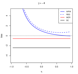
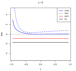
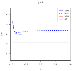
Figure 2: Sensitivity analysis for nondifferential substitution. AIPW: proposed AIPW type estimator; REG: proposed regression estimatior; WZR: Wang et al., (2017); SC: survivor-case.

In summary, the proposed AIPW type estimator is asymptotically unbiased when Assumptions 1–6 hold and is robust to model misspecification. Even if nondifferential substitution is violated, sensitivity analysis can help assess the influence of such violation. More simulation and a sensitivity analysis for monotonicity are provided in Supplementary Material E.

5 Application to allogeneic stem cell transplantation data

We first explain that Assumptions 1–3 hold. According to association analyses (Chang et al., , 2020), three binary baseline covariates, namely minimal residual disease (MRD) presence ($X_{1}=1$ for positive and 0 for negative), disease status ($X_{2}=1$ for CR1 and 0 for CR$>$1), and diagnosis ($X_{3}=1$ for T-ALL and 0 for B-ALL), were found to be related with relapse. Another post-treatment biomarker, chronic graft versus host disease (GVHD), was also shown to be associated with relapse. To avoid philosophical etiology of controlling post-treatment variables, we use potential NRMs as a reflection of GVHD since GVHD is a source of NRM. Thus, it is unnatural to assume explainable nonrandom survival. Now that all risk factors of relapse are collected in $X=(X_{1},X_{2},X_{3})$ and $(S(1),S(0))$, we expect latent ignorability to hold. Monotonicity holds because MSDT has fewer mismatched HLA loci than haplo-SCT, leading to lower NRM. Positivity holds because survival and mortality exist in both groups.

We choose age as the substitutional variable $V$. Association studies have indicated that older people have a higher probability of NRM because older people are more vulnerable to infection after surgery. However, age is not considered as a risk factor of relapse because the occurrence of relapse is more a result of biological progression. Hangai et al., (2019) found that age has a significant effect on NRM but an insignificant effect on relapse by categorizing transplantation receivers according to age. Even if age could influence relapse, it is deemed that age should have similar effects on $Y(1)$ and $Y(0)$ in all survivors because there is no biological mechanism indicating pleiotropy for age between different transplant modalities. The same result was confirmed using our dataset; see Supplementary Material F.

Table 3 displays the estimated risk difference of transplantation types on leukemia relapse (SACEC). All methods give positive point estimates, which is a sign that haplo-SCT has a lower leukemia relapse rate than MSDT. This result is consistent with clinical experience (Chang et al., , 2017, 2020). Although haplo-SCT leads to heavier GVHD and hence a higher probability of NRM, such GVHD inhibits progression of leukemia cells. The standard error of the AIPW type estimator is large, and the confidence interval of SACEC covers zero, probably because the substitutional variable is weak. Nevertheless, non-inferiority of haplo-SCT compared with MSDT in terms of leukemia relapse is concluded. The survivor-case analysis yields a smaller standard error because it does not consider the dependence of potential relapses on potential NRMs. Wang et al., (2017)’s estimator may be biased due to violation of ignorability.

Table 3: Estimated risk difference (SACEC), with standard error (s.e.) and 95% bootstrap confidence interval

Method	SACEC estimate (s.e.)	95% Confidence interval
Survivor-case analysis	0.0703 (0.0298)	(0.0118, 0.1288)
Wang et al., (2017)	0.0999 (0.3020)	(-0.2022, 0.4020)
Regression	0.1522 (0.0995)	(-0.0428, 0.3472)
AIPW type	0.1292 (0.1291)	(-0.1240, 0.3824)

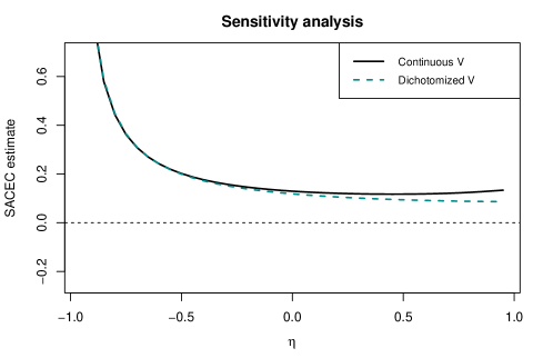
Figure 3: Sensitivity analysis of the AIPW type estimator on the stem cell transplantation data.

To perform a sensitivity analysis, Figure 3 displays the curve of estimated SACEC varying the sensitivity parameter $\eta\in(-1,1)$. We also tried a dichotomized $V$ cut at its mean to assess the robustness of the SACEC estimate to $V$. The point estimates of SACEC are always positive, indicating that the substantive conclusion is insensitive to moderate deviation from the nondifferential substitution assumption. In a nutshell, haplo-SCT is a non-inferior alternative to MSDT in terms of leukemia relapse. With the maturing intervention on survival, haplo-SCT could be a promising choice in the future.

6 Discussion

In this study, we examined the identification and estimation of causal effects when outcomes are truncated by death, where both (a) the treatment assignment and survival process, and (b) the survival process and outcome process are confounded. It is not straightforward to extend the identification results for the SACE directly from randomized experiments to observational data because the proportion of always-survivors is not always identifiable. We emphasize that the violation of explainable nonrandom survival (principal ignorability) is the key obstacle to identifying the causal effect. A substitutional variable for $S(0)$, i.e., a proxy of always-survivorship, is required to recover the information regarding the principal strata. The proposed method significantly improves the utility of real-world data and provides convenience for post-marketing drug safety and effectiveness assessments.

The introduction of a substitutional variable is similar to proximal causal inference using negative control variables (Tchetgen Tchetgen et al., , 2020; Cui et al., , 2020) or auxiliary variables (Miao et al., , 2022), but there are some important differences. First, the target estimand in the truncation-by-death setting is the local effect (i.e., the causal effect in always-survivors) rather than the overall effect. Second, we only use one variable related with the principal strata to recover the information in the principal strata. With only a single substitutional variable, the choice can be more flexible. Third, the substitutional variable is for the principal strata rather than unmeasured confounders. Finding a risk factor of $S(0)$ is easier than finding proxies of unmeasured confounders which must be rich enough to recover all the information in unmeasured confounders. If there are several eligible substitutional variables, all these variables can be involved in the regressions.

The proposed method to identify the SACEC still bears some limitations becasue it relies on untestable assumptions. Latent ignorability implies that the confounding effect between the treatment assignment and outcome process can be adjusted by principal strata and observed covariates. Latent ignorability is likely to hold if as many predictors of the treatment and outcome as possible are controlled. The nondifferential substitution assumption may be strong in some scenarios. Sensitivity analysis should be conducted when there are no external information to determine the survivorship odds ratio $\rho(v,x)$. The assumptions we adopt are the minimum requirements to identify causal effects with a single substitutional variable. Although it is possible to achieve identification of the constitution of principal strata without nondifferential substitution by double proxies for the unmeasured confounder $U$, other assumptions on the proxies like exclusion restriction or confounding bridge should be made instead (Luo et al., , 2022).

Supplementary Material

The Supplememtary Material, which includes causal graphs, proofs of theorems, additional simulation and data analysis results, is available online. Data and R codes are available at https://github.com/naiiife/TruncDeath.

Supp.pdf,1-23

References

- Chang et al., (2017) Chang, Y.-J., Wang, Y., Liu, Y.-R., Xu, L.-P., Zhang, X.-H., Chen, H., Chen, Y.-H., Wang, F.-R., Han, W., Sun, Y.-Q., et al. (2017). Haploidentical allograft is superior to matched sibling donor allograft in eradicating pre-transplantation minimal residual disease of aml patients as determined by multiparameter flow cytometry: a retrospective and prospective analysis. Journal of hematology & oncology, 10(1):1–13.
- Chang et al., (2020) Chang, Y.-J., Wang, Y., Xu, L.-P., Zhang, X.-H., Chen, H., Chen, Y.-H., Wang, F.-R., Sun, Y.-Q., Yan, C.-H., Tang, F.-F., et al. (2020). Haploidentical donor is preferred over matched sibling donor for pre-transplantation mrd positive all: a phase 3 genetically randomized study. Journal of hematology & oncology, 13(1):1–13.
- Chernozhukov et al., (2018) Chernozhukov, V., Chetverikov, D., Demirer, M., Duflo, E., Hansen, C., Newey, W., and Robins, J. (2018). Double/debiased machine learning for treatment and structural parameters: Double/debiased machine learning. The Econometrics Journal, 21(1).
- Chiba, (2011) Chiba, Y. (2011). The large sample bounds on the principal strata effect with application to a prostate cancer prevention trial. International Journal of Biostatistics, 8(1).
- Chiba and VanderWeele, (2011) Chiba, Y. and VanderWeele, T. J. (2011). A simple method for principal strata effects when the outcome has been truncated due to death. American journal of epidemiology, 173(7):745–751.
- Cui et al., (2020) Cui, Y., Pu, H., Shi, X., Miao, W., and Tchetgen Tchetgen, E. J. (2020). Semiparametric proximal causal inference. arXiv preprint arXiv:2011.08411.
- Ding et al., (2011) Ding, P., Geng, Z., Yan, W., and Zhou, X.-H. (2011). Identifiability and estimation of causal effects by principal stratification with outcomes truncated by death. Journal of the American Statistical Association, 106(496):1578–1591.
- Ding and Lu, (2017) Ding, P. and Lu, J. (2017). Principal stratification analysis using principal scores. Journal of the Royal Statistical Society: Series B (Statistical Methodology), 79(3):757–777.
- Egleston et al., (2007) Egleston, B. L., Scharfstein, D. O., Freeman, E. E., and West, S. K. (2007). Causal inference for non-mortality outcomes in the presence of death. Biostatistics, 8(3):526–545.
- Egleston et al., (2009) Egleston, B. L., Scharfstein, D. O., and MacKenzie, E. (2009). On estimation of the survivor average causal effect in observational studies when important confounders are missing due to death. Biometrics, 65(2):497–504.
- Frangakis and Rubin, (2002) Frangakis, C. E. and Rubin, D. B. (2002). Principal stratification in causal inference. Biometrics, 58(1):21–29.
- Gilbert et al., (2003) Gilbert, P. B., Bosch, R. J., and Hudgens, M. G. (2003). Sensitivity analysis for the assessment of causal vaccine effects on viral load in hiv vaccine trials. Biometrics, 59(3):531–541.
- Hangai et al., (2019) Hangai, M., Urayama, K. Y., Tanaka, J., Kato, K., Nishiwaki, S., Koh, K., Noguchi, M., Kato, K., Yoshida, N., Sato, M., et al. (2019). Allogeneic stem cell transplantation for acute lymphoblastic leukemia in adolescents and young adults. Biology of Blood and Marrow Transplantation, 25(8):1597–1602.
- Hayden et al., (2005) Hayden, D., Pauler, D. K., and Schoenfeld, D. (2005). An estimator for treatment comparisons among survivors in randomized trials. Biometrics, 61(1):305–310.
- Imai, (2008) Imai, K. (2008). Sharp bounds on the causal effects in randomized experiments with “truncation-by-death”. Statistics & probability letters, 78(2):144–149.
- Jemiai et al., (2007) Jemiai, Y., Rotnitzky, A., Shepherd, B. E., and Gilbert, P. B. (2007). Semiparametric estimation of treatment effects given base-line covariates on an outcome measured after a post-randomization event occurs. Journal of the Royal Statistical Society: Series B (Statistical Methodology), 69(5):879–901.
- Jiang and Ding, (2021) Jiang, Z. and Ding, P. (2021). Identification of causal effects within principal strata using auxiliary variables. Statistical Science, 36(4):493–508.
- Kédagni, (2021) Kédagni, D. (2021). Identifying treatment effects in the presence of confounded types. Journal of Econometrics.
- Long and Hudgens, (2013) Long, D. M. and Hudgens, M. G. (2013). Sharpening bounds on principal effects with covariates. Biometrics, 69(4):812–819.
- Luo et al., (2022) Luo, S., Li, W., Miao, W., and He, Y. (2022). Identification and estimation of causal effects in the presence of confounded principal strata. arXiv preprint arXiv:2206.08228.
- Ma et al., (2021) Ma, R., Xu, L.-P., Zhang, X.-H., Wang, Y., Chen, H., Chen, Y.-H., Wang, F.-R., Han, W., Sun, Y.-Q., Yan, C.-H., Tang, F.-F., Mo, X.-D., Liu, Y.-R., Liu, K.-Y., Huang, X.-J., and Chang, Y.-J. (2021). An integrative scoring system mainly based on quantitative dynamics of minimal/measurable residual disease for relapse prediction in patients with acute lymphoblastic leukemia. https://library.ehaweb.org/eha/2021/eha2021-virtual-congress/324642.
- McConnell et al., (2008) McConnell, S., Stuart, E. A., and Devaney, B. (2008). The truncation-by-death problem: what to do in an experimental evaluation when the outcome is not always defined. Evaluation Review, 32(2):157–186.
- McGuinness et al., (2019) McGuinness, M. B., Kasza, J., Karahalios, A., Guymer, R. H., Finger, R. P., and Simpson, J. A. (2019). A comparison of methods to estimate the survivor average causal effect in the presence of missing data: a simulation study. BMC medical research methodology, 19(1):1–14.
- Miao et al., (2022) Miao, W., Hu, W., Ogburn, E. L., and Zhou, X.-H. (2022). Identifying effects of multiple treatments in the presence of unmeasured confounding. Journal of the American Statistical Association, pages 1–15.
- Rubin, (2000) Rubin, D. B. (2000). Discussion of causal inference without counterfactuals. Journal of the American Statistical Association, 95:435–438.
- Rubin, (2006) Rubin, D. B. (2006). Causal inference through potential outcomes and principal stratification: application to studies with “censoring” due to death. Statistical Science, 21(3):299–309.
- Shepherd et al., (2006) Shepherd, B. E., Gilbert, P. B., Jemiai, Y., and Rotnitzky, A. (2006). Sensitivity analyses comparing outcomes only existing in a subset selected post-randomization, conditional on covariates, with application to hiv vaccine trials. Biometrics, 62(2):332–342.
- Tchetgen Tchetgen, (2014) Tchetgen Tchetgen, E. J. (2014). Identification and estimation of survivor average causal effects. Statistics in medicine, 33(21):3601–3628.
- Tchetgen Tchetgen et al., (2020) Tchetgen Tchetgen, E. J., Ying, A., Cui, Y., Shi, X., and Miao, W. (2020). An introduction to proximal causal learning. arXiv preprint arXiv:2009.10982.
- Wang et al., (2017) Wang, L., Zhou, X.-H., and Richardson, T. S. (2017). Identification and estimation of causal effects with outcomes truncated by death. Biometrika, 104(3):597–612.
- Yang and Small, (2016) Yang, F. and Small, D. S. (2016). Using post-outcome measurement information in censoring-by-death problems. Journal of the Royal Statistical Society: Series B: Statistical Methodology, pages 299–318.
- Zhang and Rubin, (2003) Zhang, J. L. and Rubin, D. B. (2003). Estimation of causal effects via principal stratification when some outcomes are truncated by “death”. Journal of Educational and Behavioral Statistics, 28(4):353–368.