OU-HEP-210330

New angular (and other) cuts
to improve the higgsino signal at the LHC

Howard Baer¹, Vernon Barger², Dibyashree Sengupta³ and Xerxes Tata^4
1Homer L. Dodge Department of Physics and Astronomy,
University of Oklahoma, Norman, OK 73019, USA
²Department of Physics, University of Wisconsin, Madison, WI 53706 USA
³Department of Physics, National Taiwan University, Taipei, Taiwan 10617, R.O.C.
⁴Department of Physics and Astronomy, University of Hawaii, Honolulu, HI, USA

Motivated by the fact that naturalness arguments strongly suggest that the SUSY-preserving higgsino mass parameter $\mu$ cannot be too far above the weak scale, we re-examine higgsino pair production in association with a hard QCD jet at the HL-LHC. We focus on $\ell^{+}\ell^{-}+\not\!\!\!{E_{T}}+j$ events from the production and subsequent decay, $\tilde{\chi}_{2}^{0}\rightarrow\tilde{\chi}_{1}^{0}\ell^{+}\ell^{-}$, of the heavier neutral higgsino. The novel feature of our analysis is that we suggest angular cuts to reduce the important background from $Z(\rightarrow\tau\tau)+j$ events more efficiently than the $m_{\tau\tau}^{2}<0$ cut that has been used by the ATLAS and CMS collaborations. Other cuts, needed to reduce backgrounds from $t\bar{t}$, $WWj$ and $W/Z+\ell\bar{\ell}$ production, are also delineated. We plot out the reach of LHC14 for 300 and 3000 fb^-1 and also show distributions that serve to characterize the higgsino signal, noting that higgsinos may well be the only superpartners accessible at LHC14 in a well-motivated class of natural SUSY models.

1 Introduction

1.1 Motivation

The discovery of a very Standard Model (SM)-like Higgs boson with mass $m_{h}=125.10\pm 0.14$ GeV[1, 2] at the CERN Large Hadron Collider (LHC) is a great triumph. However, it also exacerbated a long-known puzzle: what stabilizes the mass of a fundamental scalar particle when quantum corrections should drive its mass far beyond its measured value?[3, 4] The simplest and perhaps the most elegant answer is that the weak scale effective field theory (EFT) exhibits softly broken supersymmetry, and so has no quadratic sensitivity to high scale physics [5]. The electroweak scale is stabilized as long as soft supersymmetry breaking terms (at least those involving sizeable couplings to the Higgs sector) are not much larger than the TeV scale. The corresponding superpartners are then expected to have masses around the weak scale [6]. Up to now LHC superparticle searches[7] have turned up negative, resulting in lower mass limits on the gluino of $m_{\tilde{g}}\gtrsim 2.2$ TeV[8] and on the lightest top-squark $m_{\tilde{t}_{1}}\gtrsim 1.1$ TeV[9]: these bounds are obtained within simplified models, assuming that 1. the sparticle spectrum is not compressed, 2. $R$-parity is conserved and 3. gluinos and top-squarks dominantly decay to third generation quarks/squarks (as expected in the scenarios considered here[10]). Such strong limits are well beyond early expectations for sparticle masses from naturalness wherein $m_{\tilde{g}},\ m_{\tilde{t}_{1}}\lesssim 0.4$ TeV was expected (assuming 3% finetuning)[11, 12, 13, 14]. This disparity between theoretical expectations and experimental reality has caused strong doubts to be raised on the validity of the weak scale SUSY (WSS) hypothesis[18]. While there is no question that supersymmetry elegantly resolves the big hierarchy issue, the question often raised is: does WSS now suffer from a Little Hierarchy Problem (LHP), wherein a putative mass gap has opened up between the weak scale and the soft SUSY breaking scale?

The LHP seemingly depends on how naturalness is measured in WSS. The original log-derivative measure [11, 12] $\Delta_{BG}=max_{i}|\partial\log m_{Z}^{2}/\partial\log p_{i}|$ (wherein the $p_{i}$ constitute the various independent free parameters of the low energy effective field theory in question), obviously depends on one’s choice for these parameters $p_{i}$. In Ref’s [11, 12, 13, 14], the EFT was chosen to be constrained supersymmetric standard models (CMSSM or NUHM2) valid up to energy scale $Q=m_{GUT}$ and the free parameters were taken to be various GUT scale soft SUSY breaking terms such as common scalar mass $m_{0}$, common gaugino mass $m_{1/2}$, common trilinear $A_{0}$ etc. The various independent soft terms are introduced to parametrize our ignorance of how SUSY breaking is felt by the superpartners of SM particles. However, if the CMSSM is derived from a more ultra-violet complete theory (e.g string theory), then typically the EFT free parameters are determined in terms of more fundamental parameters such as the gravitino mass $m_{3/2}$ (in the case of gravity-mediation). With a reduction in independent soft parameters, parameters originally taken to be independent become correlated, and the numerical fine-tuning value can change abruptly, even for exactly the same numerical inputs[15, 16, 17]. Ignoring such correlations can lead to an over-estimate of the fine-tuning by as much as two orders of magnitude [16] and, perhaps, lead us to discard perfectly viable models for the wrong reason. An alternative measure, $\Delta_{HS}\sim\delta m_{H_{u}}^{2}/m_{h}^{2}\sim\frac{3f_{t}^{2}}{16\pi^{2}}m_{\tilde{t}}^{2}\log(\Lambda^{2}/m_{\tilde{t}}^{2})$ (which favors top-squarks $m_{\tilde{t}_{1}}\lesssim 500$ GeV), turns out to be greatly oversimplified in that it singles out one top-squark loop contribution, again ignoring the possibility of underlying cancellations in models with correlated parameters[15, 16, 17].

A more conservative, parameter-independent measure $\Delta_{EW}$ was proposed[19, 20] which directly compares the magnitude of the weak scale $m_{Z}^{2}$ to weak scale contributions from the SUSY Lagrangian:

$$\frac{m_{Z}^{2}}{2}=\frac{m_{H_{d}}^{2}+\Sigma_{d}^{d}-(m_{H_{u}}^{2}+\Sigma_{u}^{u})\tan^{2}\beta}{\tan^{2}\beta-1}-\mu^{2}\simeq-m_{H_{u}}^{2}-\mu^{2}-\Sigma_{u}^{u}(\tilde{t}_{1,2})$$ (1)

where $\Delta_{\rm EW}=max|largest\ RHS\ contribution|/(m_{Z}^{2}/2)$. An upper limit on $\Delta_{\rm EW}$ (which we take to be $\Delta_{\rm EW}<30$) then implies that the weak scale values of $\sqrt{|m_{H_{u}}^{2}|}$ and $|\mu|$ should be $\lesssim 100-350$ GeV. This means that the soft term $m_{H_{u}}^{2}$ is driven barely negative during radiative EWSB (radiatively-driven natural SUSY, or RNS)[19, 20]. The SUSY-preserving $\mu$ term, which feeds mass to $W,\ Z,\ h$ and higgsinos, is also in the $100-350$ GeV range. Meanwhile, top-squark (and other sparticle) contributions to the weak scale are loop suppressed and can lie in the $m_{\tilde{t}_{1}}\sim 1-3$ TeV range at little cost to naturalness[21, 22]. Gluinos, which influence the value of $m_{Z}$ mainly by their influence on the top squark mass, can be as heavy as 6 TeV, or more[21, 22]. Thus, a quite natural spectrum emerges under $\Delta_{EW}$ wherein higgsinos lie at the lowest mass rungs, while stops, gluinos and electroweak gauginos may comfortably lie within the several TeV range. First/second generation squarks/sleptons may well lie in the 10-40 TeV range[20]. We mention that (modulo technical caveats) $\Delta_{\rm EW}\leq\Delta_{\rm BG}$, and further, that $\Delta_{\rm BG}$ reduces to $\Delta_{\rm EW}$ when it is computed with appropriate correlations between high scale parameters [15, 16, 17].

Although not connected directly to the main theme of this paper, we note that it has been suggested that the RNS SUSY spectra are actually to be expected from considerations of the landscape of string theory vacua, which also provides an understanding of the magnitude of the cosmological constant $\Lambda_{cc}$[23, 24]. Douglas[25], Susskind[26] and Arkani-Hamed et al.[27] argue that large soft terms should be statistically favored in the landscape by a power-law $f_{SUSY}(m_{soft})\sim m_{soft}^{2n_{F}+n_{D}-1}$ where $n_{F}$ is the number of $F$-breaking fields and $n_{D}$ is the number of $D$-breaking fields contributing to the overall SUSY breaking scale. Thus, even for the textbook case of SUSY breaking via a single $F$-term ($n_{F}=1,\ n_{D}=0$), there is already a linear draw to large soft terms. The landscape statistical draw to large soft terms must be balanced by an anthropic requirement that EW symmetry is properly broken (no charge-or-color (CCB) breaking minima in the scalar potential and that EW symmetry is actually broken)[28]. Furthermore, if the value of $\mu$ is determined by whatever solution to the SUSY $\mu$ problem is invoked[29], then $\mu$ is no longer available for finetuning and the pocket universe value of the weak scale $m_{weak}^{PU}$ should be within a factor of a few of our universe’s weak scale $m_{weak}^{OU}\simeq m_{W,Z,h}\sim 100$ GeV. In pocket universes where $m_{weak}^{PU}$ is larger than 4-5 times its observed value (remarkably, this corresponds to $\Delta_{\rm EW}\lesssim 30$), Agrawal et al.[30] have shown that nuclear physics goes awry, and atoms as we know them would not form. Thus, one expects large (but not too large) soft SUSY breaking terms, and consequently large sparticle masses (save higgsinos, which gain mass differently). Detailed calculations of Higgs and sparticle masses find $m_{h}$ pulled to a statistical peak around $m_{h}\sim 125$ GeV whilst sparticles other than higgsinos are pulled (well-) beyond current LHC reach[28, 31, 32, 33].

We stress that the top-down view of electroweak naturalness is mentioned only by way of motivation and is in no way essential for the phenomenological analysis of the higgsino signal studied in this paper. The reader who does not subscribe to stringy naturalness can simply ignore the previous paragraph. For that matter, even the bottom-up naturalness considerations that led us to focus on light higgsinos do not play any essential role for the phenomenological analysis that is suggested below. In other words, the reader not interested in any naturalness considerations can simply view the remainder of this paper as an improved analysis of how light higgsinos can be searched for at the high luminosity LHC.

In our view, naturalness considerations make it very plausible that the best hope for SUSY discovery at LHC is not via gluino or top-squark pair production, but rather via light higgsino pair production: $pp\rightarrow\widetilde{\chi}_{1}^{+}\widetilde{\chi}_{1}^{-},\ \widetilde{\chi}^{0}_{1}\widetilde{\chi}^{0}_{2},\ \widetilde{\chi}^{\pm}_{1}\widetilde{\chi}^{0}_{2}$. While the total LHC higgsino pair production cross section is substantial in the mass range $\mu\sim 100-350$ GeV[34], the problem is that very little visible energy is released in higgsino decay $\widetilde{\chi}^{\pm}_{1}\rightarrow f\bar{f}^{\prime}\widetilde{\chi}^{0}_{1}$ and $\widetilde{\chi}^{0}_{2}\rightarrow f\bar{f}\widetilde{\chi}^{0}_{1}$ (where $f$ stands for SM fermions, for the most part $e$ and $\mu$ for the signals we study in this paper) since most of the decay energy ends up in the LSP rest mass $m_{\widetilde{\chi}^{0}_{1}}$[35], unless binos and winos are also fortituously light. Requiring that the higgsinos recoil against hard initial state QCD radiation, not only provides an event trigger but also boosts the higgsino decay products to measureable energy values[36, 37, 38]. Indeed, much work has already examined these reactions, and in fact limits have already been placed on such signatures by the ATLAS[39, 40] and CMS[41, 42] collaborations.

1.2 Summary of some previous work and plan for this paper

Here, we briefly summarize several previous studies on higgsino pair production and outline how the present work examines new territory.

• In Ref. [35], higgsino pair production at LHC in the low $\mu$ scenario was first examined. In that work, the reaction $pp\rightarrow\widetilde{\chi}^{0}_{1}\widetilde{\chi}^{0}_{2}$ with $\widetilde{\chi}^{0}_{2}\rightarrow\ell^{+}\ell^{-}\widetilde{\chi}^{0}_{1}$ was explored without requiring hard initial state radiation (ISR). Instead, a soft dimuon trigger was advocated. With such a trigger, then signal and BG rates were found to be comparable and the search for collimated opposite-sign/same-flavor (OS/SF) dileptons plus MET was advocated where the signal would exhibit a characteristic bump in dilepton invariant mass with $m(\ell^{+}\ell^{-})<m_{\widetilde{\chi}^{0}_{2}}-m_{\widetilde{\chi}^{0}_{1}}$.

• In Ref. [36], Han, Kribs, Martin and Menon examined the reaction $pp\rightarrow\widetilde{\chi}^{0}_{1}\widetilde{\chi}^{0}_{2}j$, where the higgsinos recoiled against a hard QCD radiation. A hard cut $m_{\tau\tau}^{\rm HKMM}>150$ GeV was used to reduce $Z\rightarrow\tau^{+}\tau^{-}j$ background. The bump in $m(\ell^{+}\ell^{-})<m_{\widetilde{\chi}^{0}_{2}}-m_{\widetilde{\chi}^{0}_{1}}$ was displayed above SM BGs for several signal benchmark models.

• In Ref. [37], an improved $m_{\tau\tau}^{2}$ variable was defined, with a crucial $m_{\tau\tau}^{2}<0$ cut used to reject $\tau\bar{\tau}j$ events compared to signal. A very conservative $b$-jet tag efficiency of 60% resulted in a dominant $t\bar{t}$ background. The current ATLAS $b$-tag efficiency is given at 85% so that requiring no $b$-jets in BG events substantially reduces $t\bar{t}$ BG. Reach contours were plotted vs. $\mu$ for several values of $m_{1/2}$ assuming integrated luminosities up to 1000 fb^-1 in this pre-HL-LHC paper. The reach plot was extended to 3000 fb^-1 in Ref. [44].

• Ref. [38] focused on SUSY models with $\Delta m^{0}\equiv m_{\widetilde{\chi}^{0}_{2}}-m_{\widetilde{\chi}^{0}_{1}}\lesssim 5$ GeV and the well-collimated dimuon pair was regarded as a single object $\mu_{col}$. Hard $\not\!\!\!{E_{T}}>250$ GeV and $p_{T}(jet)>250$ GeV cuts were applied along with transverse mass $m_{T}(\mu_{com},\not\!\!\!{E_{T}})<50$ GeV and $\not\!\!\!{E_{T}}/p_{T}(\mu_{col})>20$. Significance $S/\sqrt{BG}$ for three examined BM points were found to range from $1.85-2.9\sigma$ for assumed integrated luminosity of 3000 fb^-1.

• The CMS collaboration examined the soft dilepton+jet+$\not\!\!\!{E_{T}}$ signature in Ref. [41] using 35.9 fb^-1 of data at $\sqrt{s}=13$ TeV. They were able to exclude values of $m_{\widetilde{\chi}^{0}_{2}}$ up to about 167 GeV for $\Delta m^{0}\sim 15$ GeV although the limit drops off as $\Delta m^{0}$ falls off below or above this central value. A follow-up paper using 139 fb^-1 of data at 13 TeV extended these limits up to $\mu\sim 200$ GeV[42].

• ATLAS examined the soft dilepton+jet+$\not\!\!\!{E_{T}}$ signature in Ref’s [39] using 36.1 fb^-1 of data at $\sqrt{s}=13$ TeV where they reported the utility of an $\not\!\!\!{E_{T}}/H_{T}(\ell)\gtrsim 5$ cut. They updated their search to 139 fb^-1 in [40]. In the latter paper, values of $m_{\widetilde{\chi}^{0}_{2}}\lesssim 200$ GeV were excluded for $\Delta m^{0}\sim 10$ GeV with a rapid drop-off below and above this value. Some signal excess was noted for low $m(\ell^{+}\ell^{-})\sim 4-12$ GeV for their signal region SR-E-med plot.

• In Ref. [45], theoretical aspects of the higgsino discovery plane $m_{\widetilde{\chi}^{0}_{2}}$ vs. $\Delta m^{0}$ were explored. It was shown that the string landscape prefers the smaller mass gap region $\Delta m^{0}\sim 4-12$ GeV with $m_{\widetilde{\chi}^{0}_{2}}\sim 100-350$ GeV. In contrast, the LHC limit on the gluino mass constrains natural models with gaugino mass unification to have $\Delta m^{0}\sim 10-25$ GeV.

Our goal in the present paper is to re-examine the promising soft OS/SF dilepton plus jets plus $\not\!\!\!{E_{T}}$ signal in light of its emerging strategic importance for natural SUSY discovery in the HL-LHC era. We provide a detailed characterization of both expected signal and dominant SM backgrounds by displaying a wide variety of distributions of various kinematic variables. We also suggest new angular cuts that are much more efficient than the currently used $m_{\tau\tau}^{2}<0$ cut in suppressing the important SM background from $Z(\rightarrow\tau\bar{\tau})+jet$ production, thus aiding in the signal search at the HL-LHC.

2 Natural SUSY benchmark points

In this section, we delineate three SUSY benchmark points (BM) that are used throughout the paper in order to compare signal strength against SM background rates. We use the computer code Isajet 7.88[46] to generate all sparticle mass spectra. The ensuing SUSY Les Houches Accord (SLHA) files are input to Madgraph[47]/Pythia[48]/Delphes[49] for event generation. We select points for varying higgsino masses, and equally importantly, with different neutralino-LSP mass gaps $\sim 4-16$ GeV. The three BM points are listed in Table 1.

Our first BM point is listed as BM1 in Table 1. It is generated from the two-extra-parameter non-universal Higgs model (NUHM2) with parameters $m_{0},\ m_{1/2},\ A_{0},\ \tan\beta,\ \mu,\ m_{A}$ $=5000\ {\rm GeV},\ 1001\ {\rm GeV},\ -8000\ {\rm GeV},\ 10,\ 150\ {\rm GeV},\ 2000\ {\rm GeV}$. It has $m_{\tilde{g}}\sim 2.4$ TeV and $m_{\tilde{t}_{1}}\sim 1.6$ TeV so is LHC allowed via gluino and top squark searches. With a relatively small value $\mu=150$ GeV and a sizeable neutralino mass gap $\Delta m^{0}\sim 12$ GeV, it is just within the 95% CL region now excluded by ATLAS[40] and CMS[42] soft dilepton searches. It is natural in that $\Delta_{EW}\sim 14$.

Our second BM point (denoted BM2) is also from NUHM2 model. It has $\mu=300$ GeV with a mass gap $m_{\widetilde{\chi}^{0}_{2}}-m_{\widetilde{\chi}^{0}_{1}}\sim 16$ GeV so is well beyond current ATLAS/CMS search limits for soft dileptons+jets+$\not\!\!\!{E_{T}}$. It has $\Delta_{EW}\sim 22$.

Our third point, listed as BM3 (GMM^′), comes from natural generalized mirage mediation model[50] where $\mu$ is used as an input (GMM^′). This model combines moduli/gravity-mediation with anomaly mediated SUSY breaking (AMSB) via a mixing factor $\alpha$, where $\alpha\rightarrow 0$ corresponds to pure AMSB and $\alpha\rightarrow\infty$ corresponds to pure gravity-mediation. It uses the gravitino mass $m_{3/2}=75$ TeV as input along with continuous factors $c_{m}$, $c_{m3}$ and $a_{3}$ related to the generation 1,2 scalar masses, generation 3 scalar masses and $A$ parameters, respectively[50]. We take $\mu=200$ GeV. Since the gaugino masses unify at the intermediate mirage unification scale $\mu_{mir}\sim 5.3\times 10^{7}$ GeV, then for a given gluino mass, the wino and bino masses will be much heavier as compared to models with unified gaugino masses such as NUHM2. This means the corresponding neutralino mass gap $m_{\widetilde{\chi}^{0}_{2}}-m_{\widetilde{\chi}^{0}_{1}}\sim 4.3$ GeV so that the $\widetilde{\chi}^{0}_{2}$ decay products will be very soft, making its search a challenge even though higgsinos are not particularly heavy. The model yields $\Delta_{EW}=26$.

Although outside of the main theme of the paper, we also list values for some low energy and dark-matter-related observables towards the bottom of Table 1.

parameter	$BM1$	$BM2$	$BM3\ (GMM^{\prime})$
$m_{0}$	5000	5000	$\textendash$
$m_{1/2}$	1001	1000	$\textendash$
$A_{0}$	-8000	-8000	$\textendash$
$\tan\beta$	10	10	10
$\mu$	150	300	200
$m_{A}$	2000	2000	2000
$m_{3/2}$	$\textendash$	$\textendash$	75000
$\alpha$	$\textendash$	$\textendash$	4
$c_{m}$	$\textendash$	$\textendash$	6.9
$c_{m3}$	$\textendash$	$\textendash$	6.9
$a_{3}$	$\textendash$	$\textendash$	5.1
$m_{\tilde{g}}$	2425.4	2422.6	2837.3
$m_{\tilde{u}_{L}}$	5295.9	5295.1	5244.6
$m_{\tilde{u}_{R}}$	5427.8	5426.5	5378.0
$m_{\tilde{e}_{R}}$	4823.7	4824.5	4813.2
$m_{\tilde{t}_{1}}$	1571.7	1578.4	1386.9
$m_{\tilde{t}_{2}}$	3772.0	3773.0	3716.7
$m_{\tilde{b}_{1}}$	3806.7	3807.6	3757.8
$m_{\tilde{b}_{2}}$	5161.2	5160.2	5107.7
$m_{\tilde{\tau}_{1}}$	4746.8	4747.5	4729.8
$m_{\tilde{\tau}_{2}}$	5088.6	5088.2	5075.7
$m_{\tilde{\nu}_{\tau}}$	5095.4	5095.0	5084.8
$m_{\widetilde{\chi}^{\pm}_{2}}$	857.1	857.6	1801.9
$m_{\widetilde{\chi}^{\pm}_{1}}$	156.6	311.6	211.1
$m_{\widetilde{\chi}^{0}_{4}}$	869.0	869.8	1809.3
$m_{\widetilde{\chi}^{0}_{3}}$	451.3	454.7	1554.4
$m_{\widetilde{\chi}^{0}_{2}}$	157.6	310.1	207.0
$m_{\widetilde{\chi}^{0}_{1}}$	145.4	293.7	202.7
$m_{h}$	124.5	124.6	125.4
$\Omega_{\widetilde{\chi}^{0}_{1}}^{std}h^{2}$	0.007	0.023	0.009
$BF(b\rightarrow s\gamma)\times 10^{4}$	3.1	3.1	3.1
$BF(B_{s}\rightarrow\mu^{+}\mu^{-})\times 10^{9}$	3.8	3.8	3.8
$\sigma^{SI}(\widetilde{\chi}^{0}_{1}p)$ (pb)	$0.23\times 10^{-8}$	$0.52\times 10^{-8}$	$0.30\times 10^{-9}$
$\sigma^{SD}(\widetilde{\chi}^{0}_{1}p)$ (pb)	$0.86\times 10^{-4}$	$0.49\times 10^{-4}$	$0.54\times 10^{-5}$
$\langle\sigma v\rangle|_{v\rightarrow 0}$ (cm3/sec)	$0.3\times 10^{-24}$	$0.1\times 10^{-24}$	$0.2\times 10^{-24}$
$\Delta_{\rm EW}$	13.9	21.7	26.0

Table 1: Input parameters and masses in GeV units for two NUHM2 model benchmark points (BM1 and BM2) and one natural mirage mediation SUSY benchmark point (BM3 (GMM’)), with $m_{t}=173.2$ GeV. The input parameters for the natural(generalized) mirage mediation model such as $\alpha$ and $c_{m}$ have been calculated from $m_{0}^{MM}$ and $m_{1/2}^{MM}$ which are taken equal to the corresponding NUHM2 model values of $m_{0}$ and $m_{1/2}$, respectively. The $c_{m}$ and $c_{m3}$ have been taken equal to each other so that masses of first/second and third generation sfermions are equal at the GUT scale so as to also match the NUHM2 models in the second and third columns of the table.

3 Calculational details

3.1 Event generation

$pp$ collision events with $\sqrt{s}=14$ TeV were generated using MadGraph 2.5.5 [47] interfaced to PYTHIA v8 [48] via the default MadGraph/PYTHIA interface with default parameters for showering and hadronization. Detector simulation is performed by Delphes using the default Delphes 3.4.2 [49] “ATLAS” parameter card.

We utilize the anti-$k_{T}$ jet algorithm [52] with $R=0.6$ (the default value in the ATLAS Delphes card) rather than the Delphes card default value, $R=0.5$. (Jet finding in Delphes is implemented via FastJet [53].) We consider only jets with transverse energy satisfying $E_{T}(jet)>40$ GeV and pseudorapidity satisfying $|\eta(jet)|<3.0$ in our analysis. We implement the default Delphes $b$-jet tagger and implement a $b$-tag efficiency of 85% [54].

The lepton identification criteria that we adopt are modified from the default version of Delphes. We identify leptons with $E_{T}>5$ GeV and within $|\eta(\ell)|<2.5$. We label them as isolated leptons if the sum of the transverse energy of all other objects (tracks, calorimeter towers, etc.) within $\Delta R=0.5$ of the lepton candidate is less than $10\%$ of the lepton $E_{T}$.

3.2 SM background processes

Using Madgraph-Pythia-Delphes, we generate $10^{5}$ signal events for each of the Table 1 benchmark points. We also evaluated SM backgrounds from

• $\tau\bar{\tau}j$ production,

• $t\bar{t}$ production,

• $WWj$ production,

• $W\ell\bar{\ell}j$ production, and

• $Z\ell\bar{\ell}j$ production,

generating $10^{5}$ events for each of the background processes except $\tau\bar{\tau}j$ and $t\bar{t}$ where we generate $10^{6}$ events and also force both the tops to decay into $e$, $\mu$ or $\tau$ leptons for the latter. For the processes containing $\ell\bar{\ell}$ (here, $\ell=e,\mu$ or $\tau$) the lepton pair is produced via the decay of a virtual photon or a $Z$-boson. For the $\tau\bar{\tau}j$ background, we allow for all possible $\tau$ decay modes and then pick out the soft same-flavor opposite sign dilepton pairs at the toy detector simulation (Delphes) level.

4 Higgsino signal analysis and SM backgrounds

For the SUSY signal from higgsinos, we generate events from the reactions $pp\rightarrow\widetilde{\chi}_{1}^{\pm}\widetilde{\chi}^{0}_{2}$, $\widetilde{\chi}^{0}_{1}\widetilde{\chi}^{0}_{2}$ and $\widetilde{\chi}_{1}^{+}\widetilde{\chi}^{-}$ where $\widetilde{\chi}^{0}_{2}\rightarrow\widetilde{\chi}^{0}_{1}\ell^{+}\ell^{-}$. The visible decay products from $\widetilde{\chi}_{1}^{\pm}$ and $\widetilde{\chi}^{0}_{2}$ decays are typically soft because of their small mass difference with the LSP.

4.1 Parton level cuts and $C1$ cuts

Our listing of the dilepton plus jet signal and various background cross sections after a series of cuts detailed below is shown in Table 2. The first entry labeled $BC$ for before cuts actually has parton level cuts implemented (at the Madgraph level) since some of the subprocesses are otherwise divergent. Also, for the backgrounds with a hard QCD ISR (labeled as $j$ in row 1), we require $p_{T}(j)>80$ GeV to efficiently generate events with a hard jet. For the backgrounds including $\gamma^{*},Z^{*}\rightarrow\ell\bar{\ell}$ ($\ell=e$ or $\mu$), we implement $m(\ell\bar{\ell})>1$ GeV to regularize the otherwise divergent photon propagator. We also require $p_{T}(\ell)>1$ GeV and $\Delta R(\ell\bar{\ell})>0.01$, again at the parton level. The $W$ daughters of top quarks in $t\bar{t}$ events are forced to decay leptonically (into $e$, $\mu$ or $\tau$), but not so the $W$-bosons in first entry of the $WWj$ column. These parton events are then fed into PYTHIA and analysed using the DELPHES detector simulation. The leading order cross sections (in $fb$), for both the signal as well as for the background, are listed in row 2 and labelled as $BC$. Here, we see the signal reactions lie in the 10-100 fb regime whilst SM backgrounds are dominated by $t\bar{t}$ and $\tau\bar{\tau}j$ production and are about 500 times larger than signal point BM1.

To select out signal events, we implement cut set C1:

• require two opposite sign, same flavour (OS/SF) isolated leptons with $p_{T}(\ell)>5$ GeV, $|\eta(\ell)|<2.5$,

• require there be at least one jet in the event; i.e., $n_{j}\geq 1$ with $p_{T}(j_{1})>100$ GeV for identified calorimeter jets,

• require $\Delta R(\ell\bar{\ell})>0.05$ (for $\ell=e$ or $\mu$),

• require $\not\!\!\!{E_{T}}>100$ GeV, and

• veto tagged $b$-jets, $n$($b$-jet)=0.

cuts/process	$BM1$	$BM2$	$BM3(GMM^{\prime})$	$\tau\bar{\tau}j$	$t\bar{t}$	$WWj$	$W\ell\bar{\ell}j$	$Z\ell\bar{\ell}j$
$BC$	83.1	9.3	31.3	43800.0	41400	9860	1150.0	311
$C1$	1.2	0.19	0.07	94.2	179	35.9	14.7	5.9
$C1+m_{\tau\tau}^{2}<0$	0.92	0.13	0.043	23.1	75.6	12.8	7.7	3.2
$C1+angle$	0.69	0.12	0.04	2.2	130	22.1	11.0	4.9
$C2$	0.29	0.049	0.019	0.13	0.99	0.49	0.18	0.14
$C3$	0.25	0.033	0.017	0.13	0.29	0.39	0.15	0.07

Table 2: Cross sections (in $fb$) for signal benchmark points and the various SM backgrounds listed in the text after various cuts. The row labelled BC denotes parton level cross sections after the requirement $p_{T}(j)>80$ GeV, along with minimal cuts implemented to regulate divergences, and also includes the leptonic branching fractions for decays of both the top quarks in the $t\bar{t}$ column. The remaining rows list the cross sections after a series of analysis cuts detailed in the text.

After C1 cuts, signal cross sections for higgsino events with exactly two OS/SF isolated leptons plus at least one jet with $P_{T}>100$ GeV and $\not\!\!\!{E_{T}}>100$ GeV, are at the $fb$ or below level while corresponding SM backgrounds lie in the $5-200$ fb range. Note that after each set of cuts, of the three BM points, BM3 has the lowest surviving signal cross section as a consequence of its tiniest $\Delta m^{0}$ mass gap which leads to very soft leptons from $\tilde{\chi}_{2}^{0}$ decay.

4.2 $m_{\tau\tau}^{2}$ vs. new angular cuts

4.2.1 $m_{\tau\tau}^{2}$ cut

We see from Table 2 that $\tau\bar{\tau}j$ and $t\bar{t}$ processes constitute the largest backgrounds after C1 cuts. For the most part, hard taus come from the decay of an on-shell high $p_{T}$ $Z$ boson recoiling against a hard QCD jet, and so are very relativistic. In the approximation that the leptons and neutrinos from the decay of each tau are all exactly collimated along the parent tau direction, we can write the momentum carried off by the two neutrinos from the decay $\tau_{1}\rightarrow\ell_{1}\bar{\nu}_{\ell_{1}}\nu_{\tau_{1}}$ of the first tau as $\xi_{1}\vec{p}(\ell_{1})$ and, similarly, as $\xi_{2}\vec{p}(\ell_{2})$ for the second tau. Momentum conservation in the plane transverse to the beams then requires that

$$-\sum_{jets}\vec{p}_{T}(j)=(1+\xi_{1})\vec{p}_{T}(\ell_{1})+(1+\xi_{2})\vec{p}_{T}(\ell_{2}).$$ (2)

These two equations can be solved for $\xi_{1}$ and $\xi_{2}$ given that $\vec{p}_{T}(j)$ and $\vec{p}_{T}(\ell_{1,2})$ are all measured, and used to evaluate the momenta of the individual taus. This then allows us to evaluate the invariant mass squared of the di-tau system which (within the collinear approximation for tau decays) is given by,

$$m_{\tau\tau}^{2}=(1+\xi_{1})(1+\xi_{2})m_{\ell\ell}^{2}.$$ (3)

We show the distribution of $m_{\tau\tau}^{2}$ for both signal events as well as for the various backgrounds in Fig. 1 after the cut set C1 and further imposing $n_{j}=1$. As expected, this peaks sharply around $m_{Z}^{2}$ for the $\tau\bar{\tau}j$ background (red histogram). In contrast, for signal and other SM background events, where the isolated lepton and $\vec{\not\!\!\!{E_{T}}}$ directions are uncorrelated, the $m_{\tau\tau}^{2}$ distributions are very broad and peak at even negative values. Thus, the $m_{\tau\tau}^{2}$ provides a very good discriminator between $\tau\bar{\tau}j$ background and signal, and has, in fact, been used in ATLAS [40] and CMS [42] for their analyses. We see, however, that a rather extensive tail from the $\tau\bar{\tau}j$ background extends to negative values and arises due to tau pair production from virtual photons, the breakdown of the collinear approximation for asymmetric $Z$ decays and finally hadronic energy mismeasurements which skew the direction of both $\vec{p}_{T}(j)$ and of $\vec{\not\!\!\!{E_{T}}}$. Thus, in accord with Ref. [37], we will require $m_{\tau\tau}^{2}<0$ in the fourth row of Table 2 after ${\bf C1}$ cuts. We see that the ditau background is reduced by a factor 4 in contrast to the signal which is reduced by 25-40%, depending on the benchmark point.

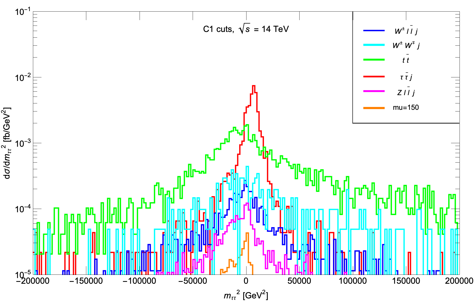
Figure 1: Distribution in $m_{\tau\tau}^{2}$ for the three SUSY BM models with $\mu=150,\ 200$ and 300 GeV introduced in the text, along with SM backgrounds after $C1$ cuts augmented by $n_{j}=1$.

Even after the $m_{\tau\tau}^{2}<0$ cut, substantial $\tau\bar{\tau}j$ background remains. We have checked that after additional cuts (described in the next section) to reduce the $t\bar{t}$ background, $\tau\bar{\tau}j$ production remains as the dominant irreducible background. This is in sharp contrast to the analysis in Ref. [37] where $t\bar{t}$ production remained as the dominant physics background even after the $m_{\tau\tau}^{2}<0$ cut. It is mainly the stronger $b$-jet veto attained by ATLAS/CMS along with further cuts described below that leads in the present case to $\tau\bar{\tau}j$ production as the dominant background. This motivated us to examine whether it is possible to reduce the di-tau background more efficiently, without a huge loss of signal. We turn to a discussion of this in Sec.4.2.2.

4.2.2 New angle cuts

In this subsection, we propose new angular cuts to replace the $m_{\tau\tau}^{2}<0$ cut that we have just discussed. In the transverse plane, the di-tau pair must recoil against the hard QCD radiation with an opening angle between the taus significantly smaller than $\pi$. The central idea, illustrated in Fig. 2, is that the $\not\!\!\!{E_{T}}$ vector must lie between the directions of the two taus which (for relativistic taus) are, of course, essentially the same as the observable directions of the charged lepton daughters of the taus. We require the azimuthal angles $\phi_{\ell}$ and $\phi_{\bar{\ell}}$ for each lepton to lie between $0$ and $2\pi$, and define $\phi_{max}=max(\phi_{\ell},\phi_{\bar{\ell}})$ and $\phi_{min}=min(\phi_{\ell},\phi_{\bar{\ell}})$. Then for $\vec{\not\!\!\!{E_{T}}}$ to lie in between the tau daughter lepton directions we must have,

$$\phi_{min}<\phi_{\hskip 2.84526pt\not\!\!\!{E_{T}}}<\phi_{max}.$$

Notice that, by definition, $\phi_{max}-\phi_{min}<\pi$, and for a boosted tau pair, often significantly smaller than $\pi$.

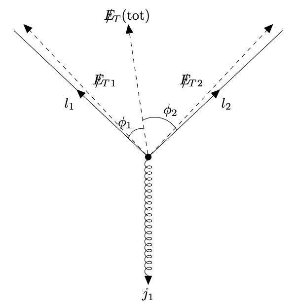
Figure 2: Sketch of a ditau background event to the di-lepton plus jet plus $\not\!\!\!{E_{T}}$ signature in the transverse plane of the event. Here $\ell_{1}$ and $\not\!\!\!{E_{T}}_{1}$ denote the transverse momentum of the lepton and of the vector sum of the neutrinos from the decay of the first tau, and likewise $\ell_{2}$ and $\not\!\!\!{E_{T}}_{2}$. $\not\!\!\!{E_{T}}$(tot) is the resultant $\not\!\!\!{E_{T}}$ in the event. Notice that because the taus are expected to be relativistic, $\ell_{i}$ and $\not\!\!\!{E_{T}}_{i}$ vectors are nearly collimated along the direction of the $i^{th}$ tau ($i=1,2$).

To characterize the $Z(\rightarrow\tau\bar{\tau})+j$ background, we show in Fig. 3 a scatter plot of these events in the $\phi_{1}\equiv\phi_{max}-\phi_{\hskip 2.84526pt\not\!\!\!{E_{T}}}$ vs. $\phi_{2}\equiv\phi_{\hskip 2.84526pt\not\!\!\!{E_{T}}}-\phi_{min}$ plane. If the collinear approximation for tau decays holds, we would expect that the $\tau\tau j$ background selectively populates the top right quadrant with $\phi_{1}>0$ and $\phi_{2}>0$ with $\phi_{1}+\phi_{2}=\phi_{max}-\phi_{min}<\pi$, and significantly smaller than $\pi$ when the tau pair emerges with a small opening angle in the transverse plane. We see from the figure that there is a small, but significant, spill-over into the region where $\phi_{1}$ or $\phi_{2}$ assumes small negative values; i.e. where $\vec{\not\!\!\!{E_{T}}}$ lies just outside the cone formed by $\vec{\ell_{1}}$ and $\vec{\ell_{2}}$. This spill-over arises from asymmetric decays of the $Z$ where one of the taus (the one emitted backwards from the $Z$ direction) is relatively less relativistic so that the collinear approximation works poorly, or because hadronic energy mismeasurements skew the direction of $\vec{\not\!\!\!{E_{T}}}$. Indeed we see from Fig. 3 that the $\tau\tau j$ background mostly populates the triangle in the top-right corner of the $\phi_{1}$ vs. $\phi_{2}$ plane, and $\phi_{1}+\phi_{2}<f\pi$ where the fraction $0<f<1$, with a spill-over into the strips where one of $\phi_{1,2}$ is slightly negative. For signal events and for the other backgrounds, $\phi_{\hskip 2.84526pt\not\!\!\!{E_{T}}}$ will be uncorrelated with $\phi_{min}$ and $\phi_{max}$, and so their scatter plots will extend to the other quadrants. This is illustrated for the $t\bar{t}$ background in Fig. 4 and for signal point BM1 in Fig. 5. In these cases, we indeed see a wide spread in $\phi_{1}$ and $\phi_{2}$ between $\pm 2\pi$.

To efficiently veto the $\tau\bar{\tau}j$ background, we have examined nine cases of angular cuts. To optimize the effect of the boost on the opening angle of the two taus, we examine three ranges of $\phi_{1}+\phi_{2}$:

• a1: $\phi_{1},\ \phi_{2}>0$,

• b1: $\phi_{1},\ \phi_{2}>0$ with $\phi_{1}+\phi_{2}<\pi/2$, and

• c1: $\phi_{1},\ \phi_{2}>0$ with $\phi_{1}+\phi_{2}<2\pi/3$.

Next, to optimize the width of the “strip” where the $\not\!\!\!{E_{T}}$ vector is allowed to stray outside the cone formed by the leptons, we also tried,

• a2, b2 and c2 where instead $\phi_{1},\ \phi_{2}>-\pi/10$, and

• a3, b3 and c3 with $\phi_{1},\ \phi_{2}>-\pi/20$.

The set which gives optimized $S/\sqrt{BG(\tau\bar{\tau}j)}$ for LHC14 with 3000 fb^-1 was found to be set b1:

$${\rm veto\ the\ triangle}\ \ \ \phi_{1},\ \phi_{2}>0\ \ {\rm with}\ \ \phi_{1}+\phi_{2}<\pi/2,$$ (4)

along with an additional veto of the $|\phi_{1}|$ and $|\phi_{2}|$ strips along the positive $\phi_{1}$ and $\phi_{2}$ axes to further reduce background from the spill-over of $\ \vec{\not\!\!\!{E_{T}}}$ outside of the cone defined by the taus that we already discussed:

$${\rm strip\ cuts:\ veto}|\phi_{1,2}|<\pi/10.$$ (5)

We list signal and background rates after C1 cuts together with the angle cuts (4) and (5) in row 5 of Table 2. In this case, we find that $\tau\bar{\tau}j$ background is reduced from cut set C1 by a factor $\sim 43$ (compared to a factor $\sim 4$ for the $m_{\tau\tau}^{2}<0$ cut) whilst signal efficiency for the point BM1 is almost 60% (compared to $\sim 75$% for the $m_{\tau\tau}^{2}<0$ cut). We also see that signal efficiency for the other two benchmark points is nearly the same for the angular and for the $m_{\tau\tau}^{2}<0$ cuts. We regard the angular cuts as a significantly improved method for reducing $\tau\bar{\tau}j$ background relative to signal. We note that the other SM backgrounds are not as efficiently reduced by the angular cut as by the $m_{\tau\tau}^{2}<0$ cut, and it is with this in mind that we turn to the examination of other distributions below.

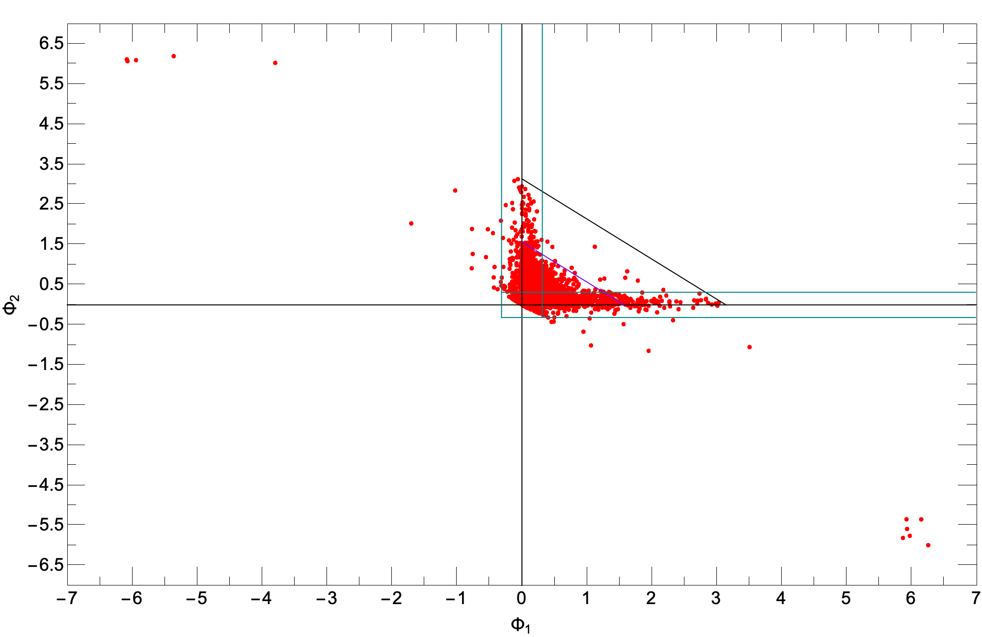
Figure 3: Distribution in $\phi_{1}$ vs. $\phi_{2}$ plane for $\tau\bar{\tau}j$ background after $C1$ cuts, rquiring also that $n_{j}=1$.

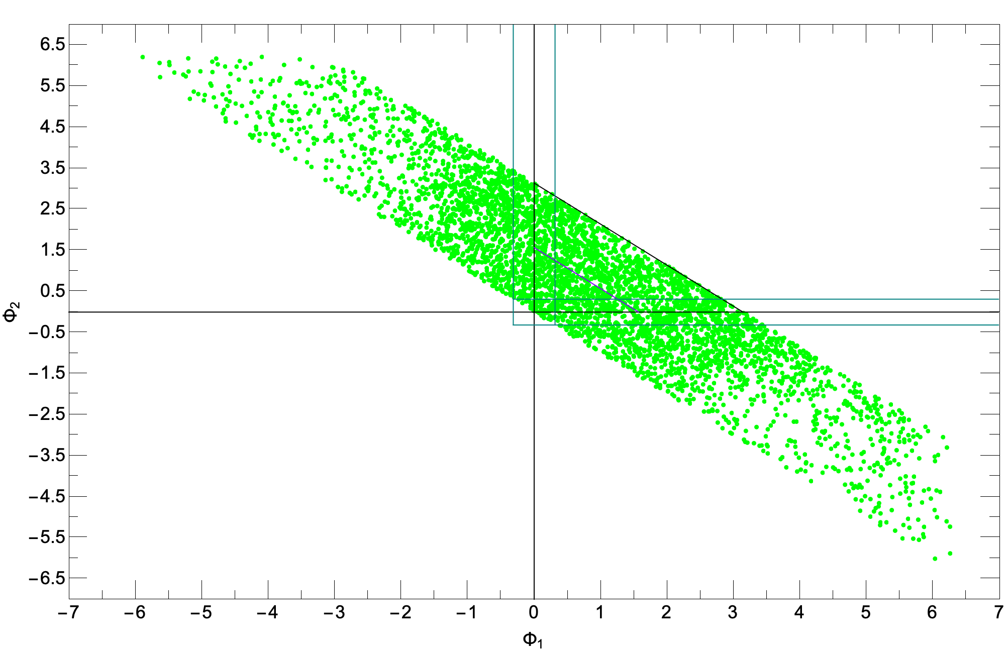
Figure 4: Distribution in $\phi_{1}$ vs. $\phi_{2}$ plane for $t\bar{t}$ background after $C1$ cuts, requiring also that $n_{j}=1$.

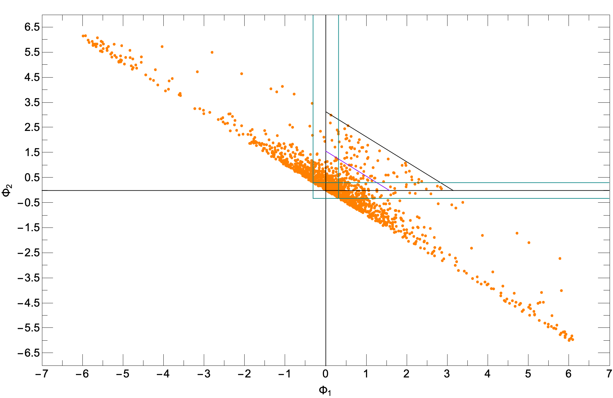
Figure 5: Distribution in $\phi_{1}$ vs. $\phi_{2}$ plane for signal point BM1 after $C1$ cuts, requiring also that $n_{j}=1$.

4.3 Additional distributions to reduce $t\bar{t}$, $WWj$ and other backgrounds

We have seen that after C1 cut set augmented by the angular cuts, the main SM backgrounds arise from $t\bar{t}$ and $WWj$ production followed by leptonic decays of the top and $W$-bosons. Since $t\bar{t}$ production leads typically to events with two hard daughter $b$-quarks, we begin with the examination of the jet multiplicity $n(jets)$ in Fig. 6. The signal distributions are shown as thick orange, black and purple histograms for the benchmark cases, BM1, BM2 and BM3, respectively, and they all feature steadily falling $n(jets)$ distribution since jets only arise from ISR. In contrast, $n(jets)$ from $t\bar{t}$ production has a rather flat distribution out to $n(jets)\sim 3$ with a steady drop-off thereafter. The other EW backgrounds also feature falling $n(jet)$ distributions. Restricting $n(jets)\sim 1-2$ should cut $t\bar{t}$ background substantially with relatively small cost to signal.

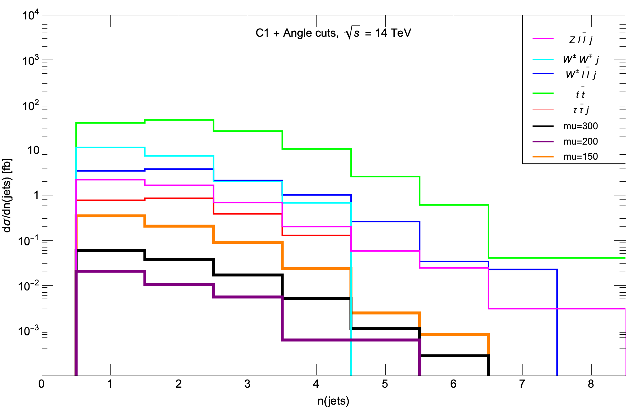
Figure 6: Distribution in $n(jet)$ for three SUSY BM models with $\mu=150,\ 200$ and 300 GeV along with SM backgrounds after $C1$ and the angular cuts described in the text.

We continue our examination by showing in Fig. 7 and Fig. 8 the distribution of the highest $p_{T}$ jet and of $\not\!\!\!{E_{T}}$, respectively, again after C1 and angular cuts. We see that both distributions are backed up against the cut and falling steeply, for both the signal cases as well as for the backgrounds. While these distributions may be falling slightly faster for the top background as compared to the signal, it is clear that requiring harder cuts on either $p_{T}(j_{1})$ or $\not\!\!\!{E_{T}}$ would greatly reduce the already small signal.

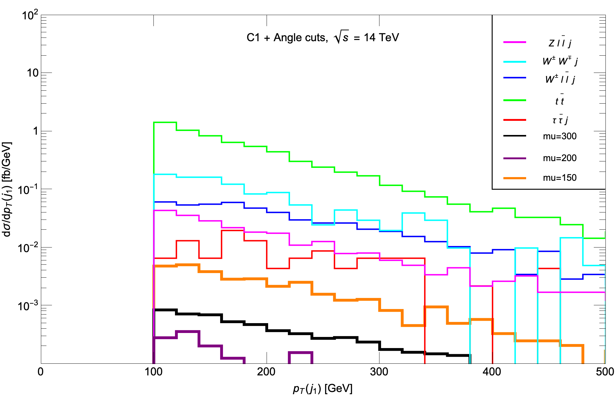
Figure 7: Distribution of the hardest jet $p_{T}(j_{1})$ for the three SUSY BM models with $\mu=150,\ 200$ and 300 GeV and for SM backgrounds after $C1$ and angular cuts.

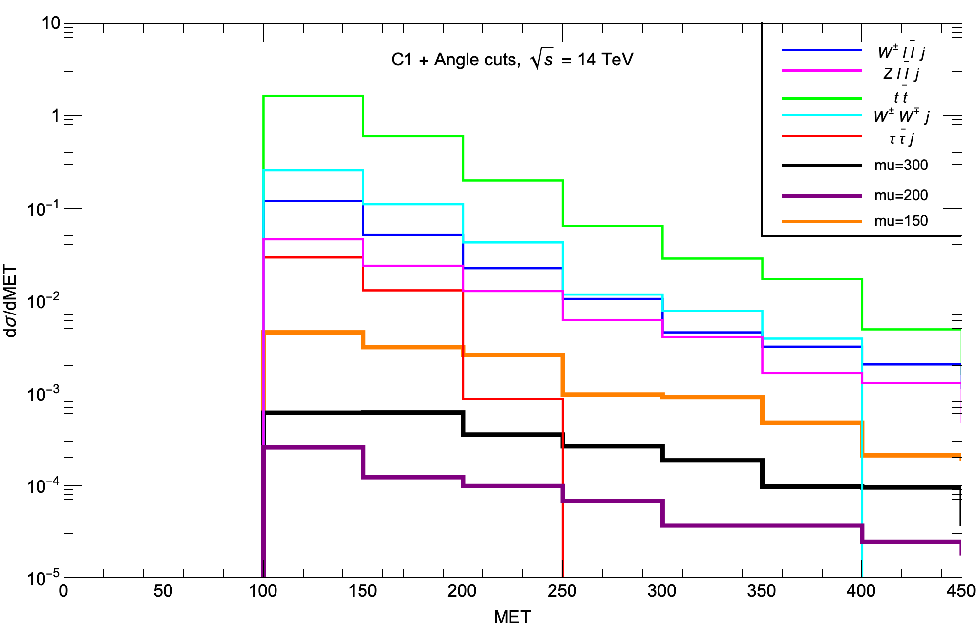
Figure 8: Distribution of $\not\!\!\!{E_{T}}$ for the three SUSY BM models with $\mu=150,\ 200$ and 300 GeV and for SM backgrounds after $C1$ and angular cuts.

Turning to the leptons in the events, we show in Fig. 9 the distributions in $p_{T}(\ell_{1})$, the highest $p_{T}$ isolated lepton. As expected, the signal distributions are very soft whereas the corresponding distributions from $t\bar{t}$, $WWj$ (and even from the residual $\tau\bar{\tau}j$ events) extend to far beyond where the signal distributions have fallen to 10-20% of their peak value. In this case, an upper bound on $p_{T}(\ell_{1})\lesssim 25-40$ GeV might be warranted, at least for SUSY signal cases where the neutralino mass gap is $\lesssim 20$ GeV.

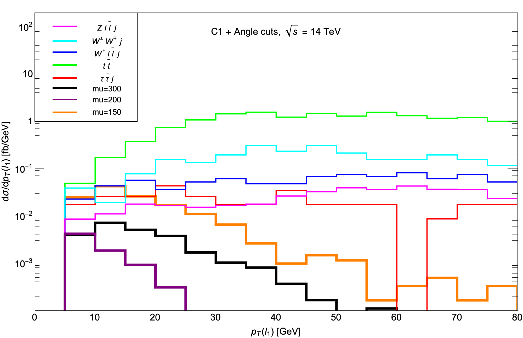
Figure 9: Distribution of the transverse momentum of the hard lepton $p_{T}(\ell_{1})$ for the three SUSY BM models with $\mu=150,\ 200$ and 300 GeV and for SM backgrounds after $C1$ and the angular cuts.

In Fig. 10, we show the resultant distributions in $p_{T}$ of the lower $p_{T}$ isolated lepton. In this case, the three signal BM models have sharply falling distributions whilst many of the SM background distributions are rather flat out to high $p_{T}(\ell_{2})$. Requiring $p_{T}(\ell_{2}):5-20$ GeV should save the bulk of signal events (at least as long as the neutralino mass gap is not very large) while rejecting the majority of the background.

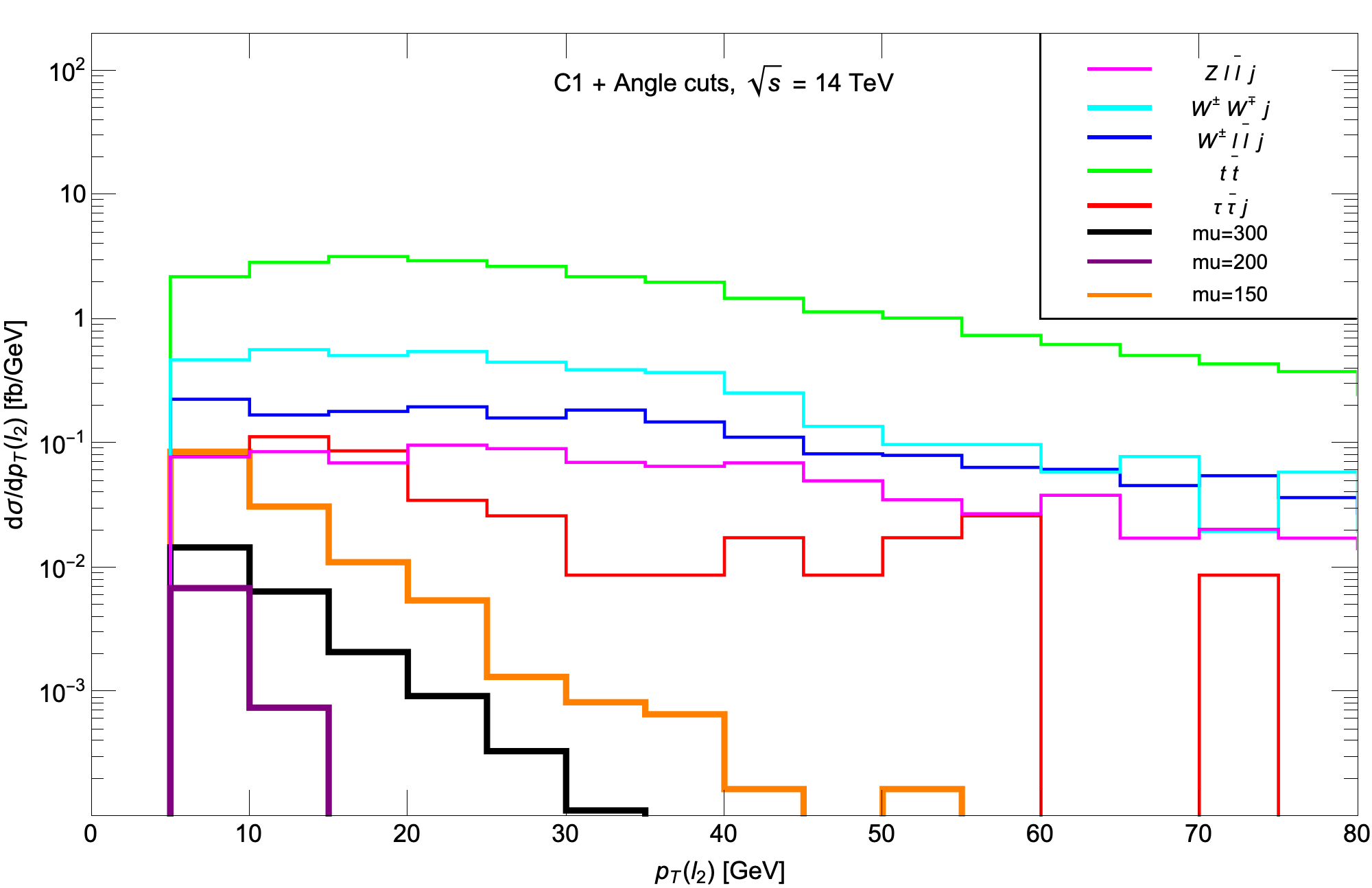
Figure 10: Distribution of the softer lepton $p_{T}(\ell_{2})$ for the three SUSY BM models with $\mu=150,200$ and 300 GeV SUSY BM models and for SM backgrounds after $C1$ and angular cuts.

In Fig. 11, we plot the scalar sum of lepton $p_{T}$ values $H_{T}(\ell\bar{\ell})\equiv|p_{T}(\ell_{1})|+|p_{T}(\ell_{2})|$. Since signal gives rise to soft OS/SF dileptons while most backgrounds have at least one hard lepton, then we expect harder $H_{T}$ distributions from background. The figure illustrates that this is indeed the case, and that a cut $H_{T}(\ell\bar{\ell})\lesssim 50-60$ GeV would enhance the signal relative to the background. Of course, $|p_{T}(\ell_{1})|,|p_{T}(\ell_{2})|$ and $H_{T}$ are strongly correlated, so that cutting on any two of these would serve for our purpose.

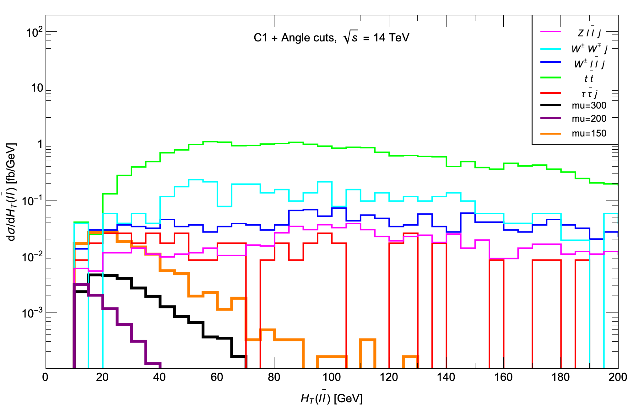
Figure 11: Distribution in $H_{T}(\ell\bar{\ell})$ for the three SUSY BM models with $\mu=150$ GeV, 200 GeV and 300 GeV and for SM backgrounds after $C1$ and angular cuts.

The distribution in $\not\!\!\!{E_{T}}/H_{T}(\ell\bar{\ell})$ was found by the ATLAS collaboration to be an effective signal-to-background discriminator in Ref. [39]. The signal is expected to exhibit a soft $H_{T}$ distribution compared to a hard $\not\!\!\!{E_{T}}$ distribution from recoil of SUSY particles against the ISR jet. Thus, signal is expected to exhibit a hard $\not\!\!\!{E_{T}}/H_{T}$ distribution compared to background. In Fig. 12, we show the relevant SUSY BM distributions along with SM backgrounds. Indeed, almost all $t\bar{t}$ events – and also most other events – lie with $\not\!\!\!{E_{T}}/H_{T}\lesssim 4$ while signal events peak around $\not\!\!\!{E_{T}}/H_{T}\sim 5-10$. We will, in addition, require $\not\!\!\!{E_{T}}/H_{T}>4$ for our next cut set C2.

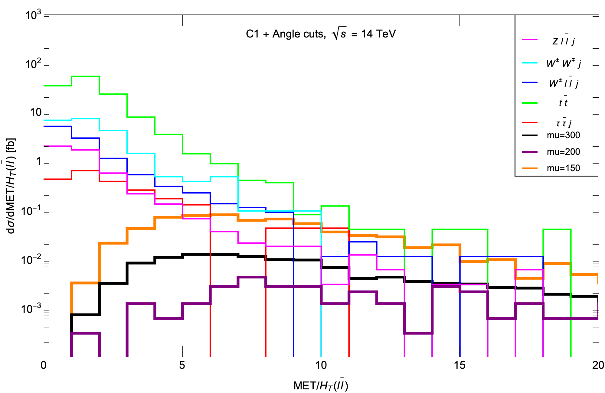
Figure 12: Distribution of $\not\!\!\!{E_{T}}/H_{T}(\ell)$ for three SUSY BM models with $\mu=150,\ 200$ and 300 GeV and for SM backgrounds after $C1$ cuts and angular cuts.

4.4 $C2$ cuts: signal, BG and distributions

In light of the distributions just discussed, we next include the following cut set C2 to enhance the higgsino signal over top, $WWj$ and the other EW backgrounds:

• the cut set C1 together with the ${\rm angle\ cuts}$,

• $n(jets)=1$,

• $p_{T}(\ell_{2}):5-15$ GeV,

• $H_{T}(\ell\bar{\ell})<60$ GeV

• $\not\!\!\!{E_{T}}/H_{T}(\ell\bar{\ell})>4$, and

• $m(\ell\bar{\ell})<50$ GeV.

The reader will have noticed that we have included an upper limit on the invariant mass of the dilepton pair. This cut is motivated from the fact that the invariant mass distributions of dileptons from $\widetilde{\chi}^{0}_{2}\rightarrow\widetilde{\chi}^{0}_{1}\ell\bar{\ell}$ decay is kinematically bounded by $m_{\widetilde{\chi}^{0}_{2}}-m_{\widetilde{\chi}^{0}_{1}}$, and further that leptons from the decays of different charginos/neutralinos also tend to have small energies (and hence also small $m(\ell\bar{\ell})$) because the higgsino spectrum is compressed. In contrast, leptons from decays of background tops and $W$-bosons tend to be hard (see Fig. 9 and Fig. 10) and, because the lepton directions are uncorrelated, the corresponding background dilepton mass distributions are relatively flat out to very large values of $m(\ell\bar{\ell})$. Although we do not show it, we have checked that the requirement $m(\ell\bar{\ell})<50$ GeV, efficiently reduces much of the background while retaining most of the higgsino signal as long as the higgsino spectrum is compressed.

We see from the penultimate row of Table 2 that after C2 cuts, the leading $t\bar{t}$ background has dropped by a factor $\sim 130$, and the total SM background has dropped to $\sim 1.1$%, while the signal is retained with an efficiency of 40-60%. At this point, the total background is just below 2 fb. Clearly, the signal cross section is small, and the large integrated luminosities expected at the HL-LHC will be necessary for the detection of the signal if the higgsino mass is close to its naturalness bound of 300-350 GeV, or if the higgsino spectrum is maximally compressed, consistent with naturalness.

To characterize the signal events, and further improve the discrimination of the signal vis-a-vis the background, we examine other distributions after C2 cuts, starting with the dilepton invariant mass distribution in Fig. 13. We can gauge that the SM background distribution, summed over the backgrounds, is essentially flat. In contrast, the signal distributions show an accumulation of events below $m_{\widetilde{\chi}^{0}_{2}}-m_{\widetilde{\chi}^{0}_{1}}$ together with a long tail (with a much smaller number of events) where the two leptons originate in different charginos/neutralinos.

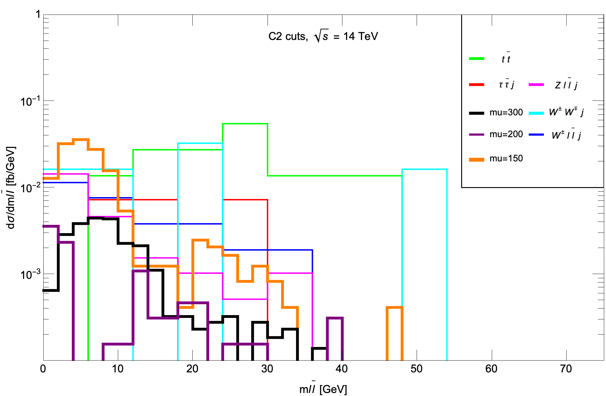
Figure 13: Distribution in $m(\ell\bar{\ell})$ for the three SUSY BM models with $\mu=150,\ 200$ and 300 GeV, and for SM backgrounds after $C2$ cuts.

In Fig. 14, we show the distribution in transverse opening angle $\Delta\phi(j_{1},\vec{\not\!\!\!{E_{T}}})$. For the signal, where the SUSY particles recoil strongly against the ISR jet, we expect nearly back-to-back $\vec{p}_{T}(jet)$ and $\vec{\not\!\!\!{E_{T}}}$ vectors. This correlation is expected to be somewhat weaker from the $W\ell\bar{\ell}j$ and especially $t\bar{t}$ backgrounds because these intrinsically contain additional activity from decay products that do not form jets or identified leptons. Indeed, requiring $\Delta\phi(\vec{p}_{T}(j_{1}),\vec{\not\!\!\!{E_{T}}})\gtrsim 2$ appears to give only a slight improvement in the signal-to-background ratio.

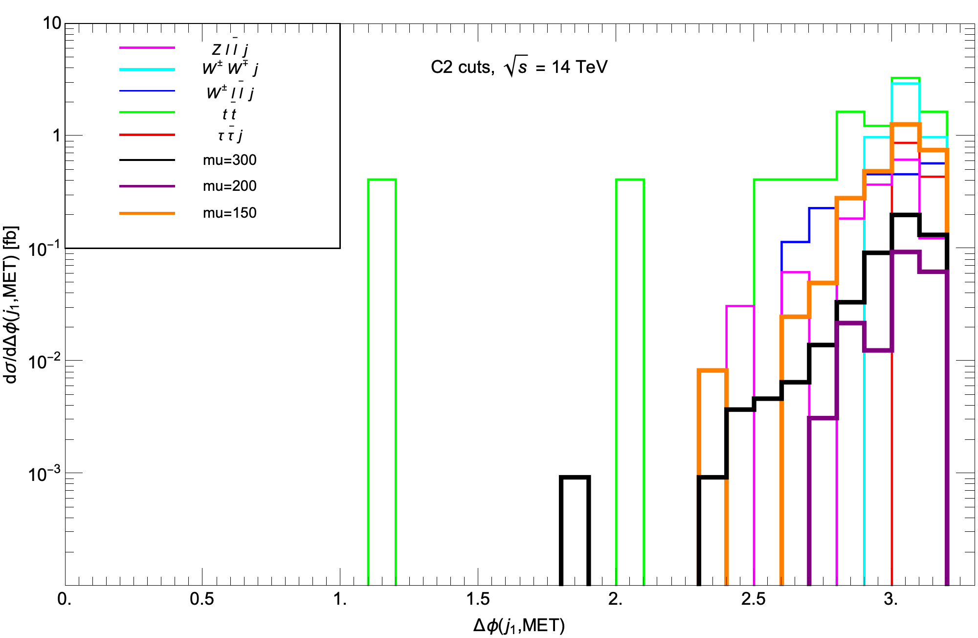
Figure 14: Distribution in $\Delta\phi(jet,\not\!\!\!{E_{T}})$ for the three SUSY BM models with $\mu=150,\ 200$ and 300 GeV, and for SM backgrounds after $C2$ cuts.

In Fig. 15, we plot the dilepton-plus-$\not\!\!\!{E_{T}}$ cluster transverse mass $m_{cT}(\ell\bar{\ell},\not\!\!\!{E_{T}})$. From the frame, we see the signal distributions all have broad peaks around 20-100 GeV while several of the backgrounds that contain harder leptons extend to well past 100 GeV. Thus, a candidate analysis cut might include $m_{cT}\lesssim 100$ GeV.

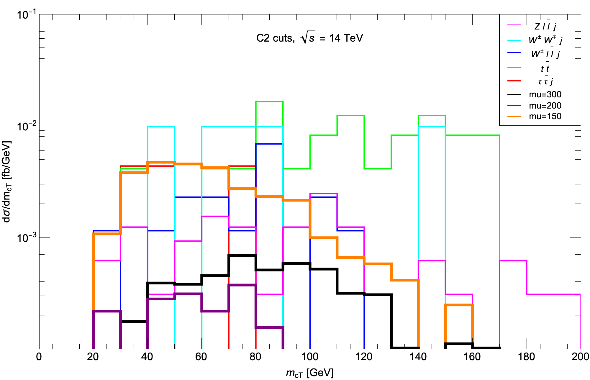
Figure 15: Distribution in $m_{cT}(\ell^{+}\ell^{-},\not\!\!\!{E_{T}})$ for the three SUSY BM models with $\mu=150,\ 200$ and 300 GeV, and for SM backgrounds after $C2$ cuts.

In Fig. 16, we plot the distribution in $p_{T}(j_{1})/\not\!\!\!{E_{T}}$. For the signal, we expect $\vec{\not\!\!\!{E_{T}}}$ to mainly recoil against the hard ISR jet so that signal would peak around $\sim 1$ since the dileptons are soft. In contrast, some of the backgrounds will include harder high-$p_{T}$ objects so this ratio is expected to be less correlated. While both signal and BGs peak around $p_{T}(j_{1})/\not\!\!\!{E_{T}}\sim 1$, we note that several BG distributions extend out to $p_{T}(j_{1})/\not\!\!\!{E_{T}}\sim 3$. Thus, we could require $p_{T}(j_{1})/\not\!\!\!{E_{T}}\lesssim 1.5$.

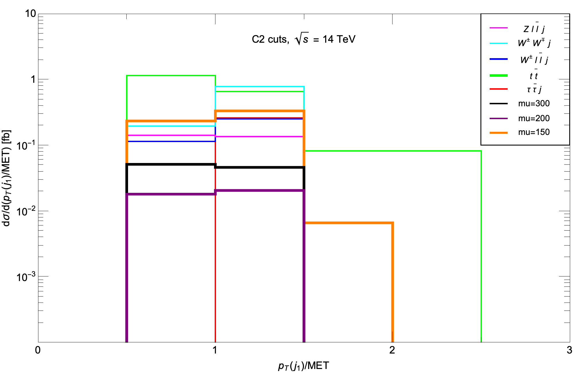
Figure 16: Distribution in $E_{T}(jet)/\not\!\!\!{E_{T}}$ for three SUSY BM models with $\mu=150,\ 200$ and 300 GeV along with SM backgrounds after $C2$ cuts.

A related distribution is to plot $p_{T}(j_{1})-\not\!\!\!{E_{T}}$, where again signal values of $p_{T}(j_{1})$ and $\not\!\!\!{E_{T}}$ are expected to be nearly equal and opposite and so should peak around $\sim 0$. The backgrounds have a similar peak structure, but extend to higher values especially in the positive direction. Therefore, we might require $|p_{T}(j_{1})-\not\!\!\!{E_{T}}|\lesssim 100$ GeV. We note though that the considerations in Figs. 14, 16 and 17 have the same underlying physics, and hence the corresponding cuts are certainly correlated.

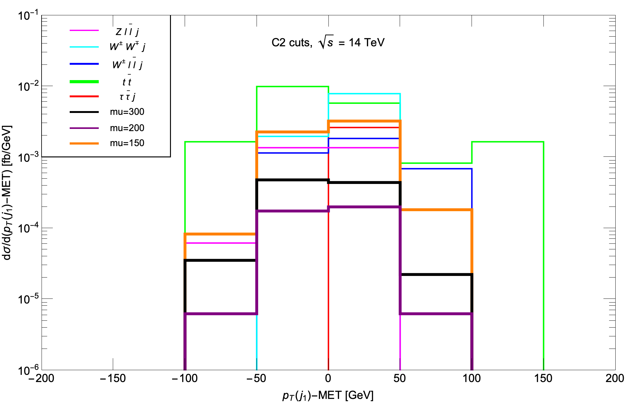
Figure 17: Distribution in $E_{T}(jet)-\not\!\!\!{E_{T}}$ for the three SUSY BM models with $\mu=150,\ 200$ and 300 GeV, and for SM backgrounds after $C2$ cuts.

In Fig. 18, we show the distribution in dimuon transverse opening angle $\Delta\phi(\mu\bar{\mu})$. In the signal case, we expect a significant recoil of $\widetilde{\chi}^{0}_{2}$ from the ISR jet so that the muon pair originating from the $\widetilde{\chi}^{0}_{2}\rightarrow\widetilde{\chi}^{0}_{1}\mu\bar{\mu}$ decay should be tightly collimated with small opening angle [38]. For the background processes, or for that matter from higgsino pair production processes, where the leptons originate from different particles or higher energy release decays, we do not expect the dilepton pair to be so collimated, and indeed the total background is (within fluctuations in our simulation) consistent with being roughly flat in $\Delta\phi(\mu\bar{\mu})$. Indeed, from the figure we see that $\Delta\phi(\mu\bar{\mu})\sim 0-1$ for signal processes while the SM BG processes tend to have opening angles less well collimated and extending well past $\Delta\phi\sim 1.5$. Although we have focussed on dimuons here, exactly the same consideration would also apply to $e^{+}e^{-}+j+\not\!\!\!{E_{T}}$ events, as long as the direction of the electrons can be reliably measured.

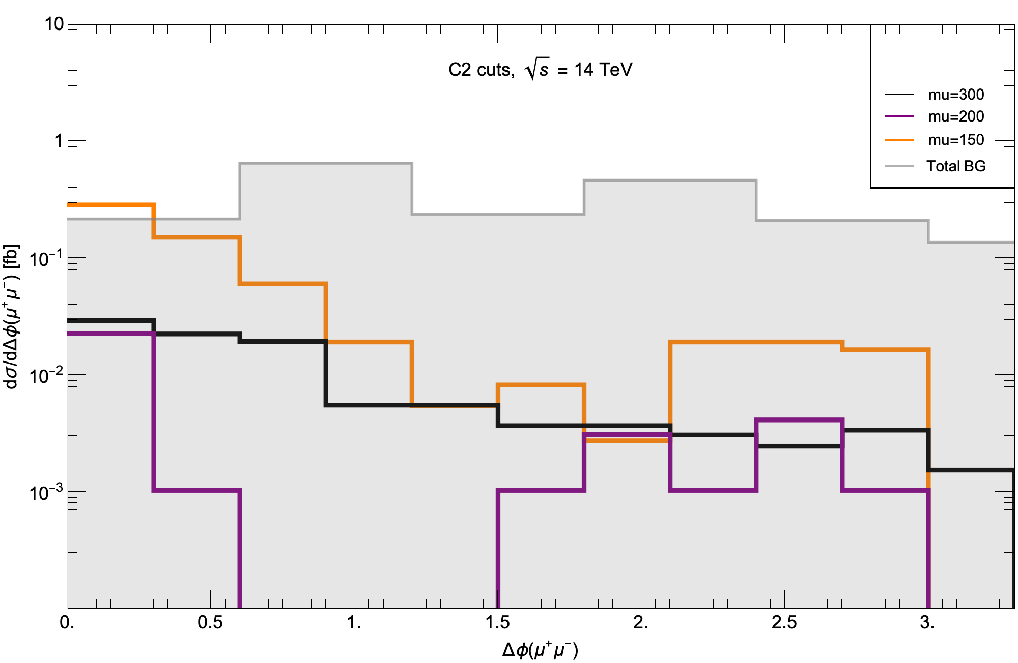
Figure 18: Distribution in $\Delta\phi(\mu\bar{\mu})$ for three SUSY BM models with $\mu=150,\ 200$ and 300 GeV along with SM backgrounds after $C3$ cuts.

In light of the above distributions, we next include the following cut set C3 that includes:

• all C2 cuts,

• $\Delta\phi(j_{1},\not\!\!\!{E_{T}})>2.0$

• $m_{cT}(\ell\bar{\ell},\not\!\!\!{E_{T}})<100$ GeV

• $p_{T}(j_{1})/\not\!\!\!{E_{T}}<1.5$

• $|p_{T}(j_{1})-\not\!\!\!{E_{T}}|<100$ GeV

The OS/SF dilepton invariant mass after these C3 cuts is shown in Fig. 19, this time on a linear scale. The total background is shown in gray, whilst signal-plus-background is the colored histogram, and correspond to a) BM1 with $\Delta m=12$ GeV, b) BM2 with $\Delta m=16$ GeV and c) BM3 with $\Delta m=4.3$ GeV. The idea here is to look for systematic deviations from SM background predictions in the lowest $m(\ell\bar{\ell})$ bins. Those bins with a notable excess could determine the kinematic limit $m(\ell\bar{\ell})<m_{\widetilde{\chi}^{0}_{2}}-m_{\widetilde{\chi}^{0}_{1}}$. By taking only the bins with a notable excess, i.e. $m(\ell\bar{\ell})<m_{\widetilde{\chi}^{0}_{2}}-m_{\widetilde{\chi}^{0}_{1}}$, then it is possible to compute the cut-and-count excess above expected background to determine a $5\sigma$ or a 95% CL limit. The shape of the distribution of the excess below the $\widetilde{\chi}^{0}_{2}\rightarrow\widetilde{\chi}^{0}_{1}\ell\bar{\ell}$ end point depends on the relative sign of the lighter neutralino eigenvalues (these have opposite signs for higginos) and so could serve to check the consistency of higgsinos as the origin of the signal[57]. Of the three cases shown, this would be possible at the HL-LHC only for the point BM1, since the tiny signal to background ratio precludes the possibility of determining the signal shape in the other two cases.

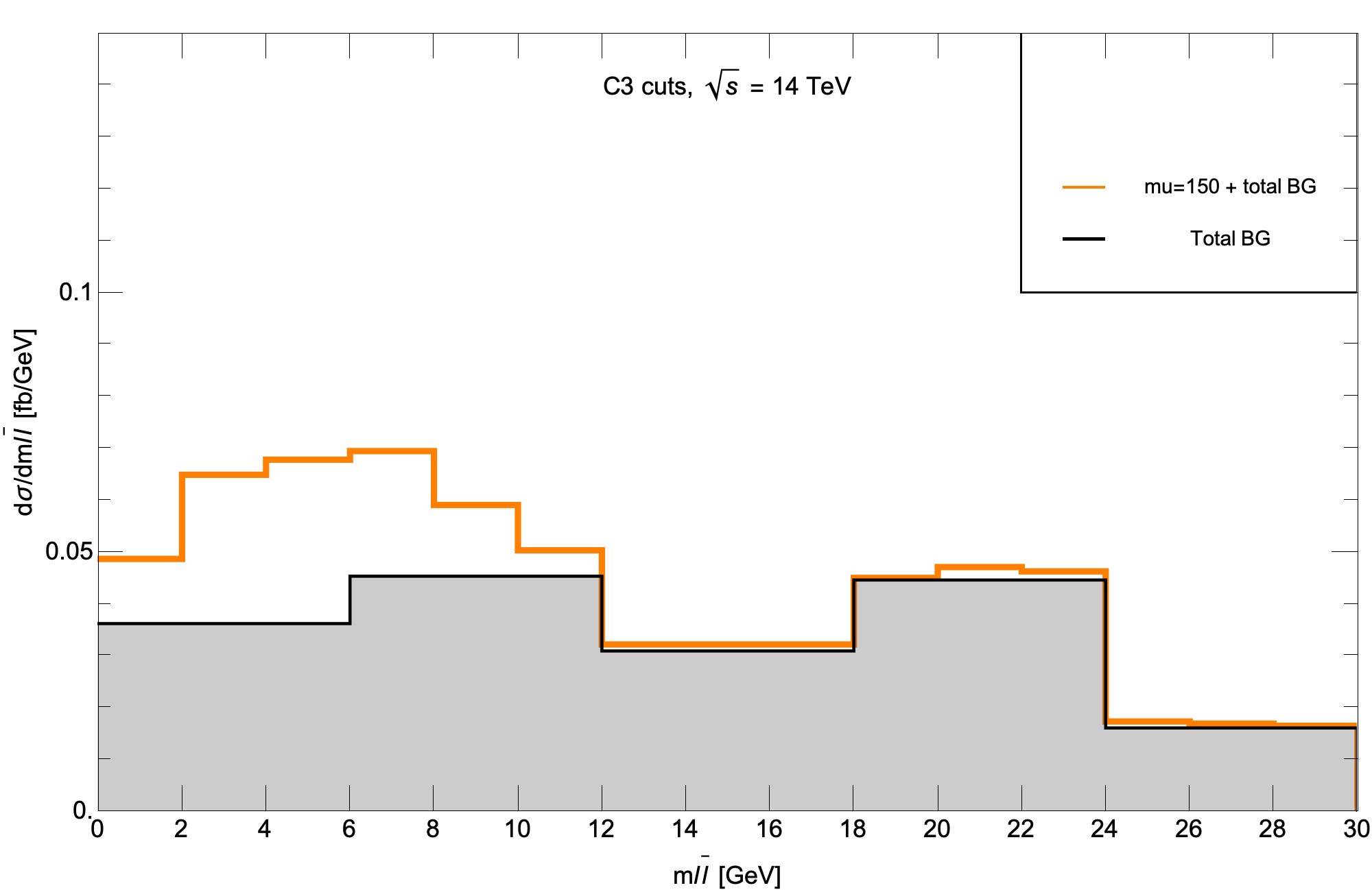
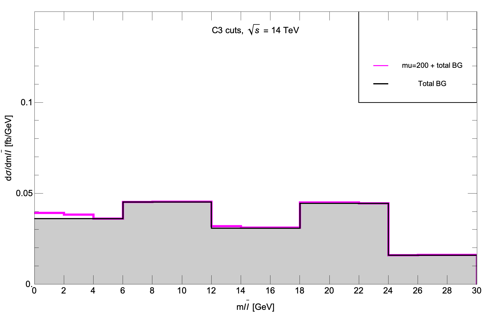
Figure 19: Distribution of $m(\ell^{+}\ell^{-})$ for the three SUSY BM models with $\mu=150,\ 300$ and 200 GeV, and for the SM backgrounds after $C3$ cuts.

5 LHC reach for higgsinos with 300-3000 fb^-1

In light of the above distributions, we next include the following cut set C4:

• apply all C3 cuts,

• then, require $m(\ell\bar{\ell})<m_{\widetilde{\chi}^{0}_{2}}-m_{\widetilde{\chi}^{0}_{1}}$.

The reader could legitimately ask how we could implement this since we do not a priori know the neutralino mass gap. The location of the mass gap can be visually seen for BM1, but would be obscured by the background for the other two cases. What we really mean is to measure the cross section with $m_{\ell\ell}<m_{\ell\ell}^{\rm cut}$, varying the value of $m_{\ell\ell}^{\rm cut}$ and looking for a rise in the (low mass) region where events from $\widetilde{\chi}^{0}_{2}\rightarrow\widetilde{\chi}^{0}_{1}\ell\bar{\ell}$ would be expected to accumulate. In the following, we will assume that once we have the data, the region where the higgsino signal is beginning to accumulate will be self-evident.

Using these C4 cuts, then we computed the remaining signal cross section after cuts for four model lines in the NUHM2 model for variable values of $\mu:100-400$ GeV and with variable $m_{1/2}$ values adjusted such that the $m_{\widetilde{\chi}^{0}_{2}}-m_{\widetilde{\chi}^{0}_{1}}$ mass gap is fixed at 4, 8, 12 and 16 GeV. While $\mu$ and $m_{1/2}$ are variable, the values of $m_{0}=5$ TeV, $A_{0}=-1.6m_{0}$, $\tan\beta=10$ and $m_{A}=2$ TeV are fixed for all four model lines. In Fig. 20, we show the signal cross section after C4 cuts, along with the $5\sigma$ reach and the 95% CL exclusion for LHC14 with 300 and 3000 fb^-1. We also list the total background in each frame in case the reader wishes to estimate the statistical significance of the signal for a given value of $m_{\tilde{\chi}_{2}^{0}}$ for different choices of integrated luminosity.

In Fig. 20a), we find for $\Delta m=4$ GeV that the $5\sigma$ (95% CL) reach of LHC14 with 300 fb^-1 extends out to 80 GeV (122 GeV) respectively. For HL-LHC with 3000 fb^-1, then we obtain the corresponding values to be 131 GeV (173.5 GeV). Thus, the HL-LHC should give us an extra reach in $\mu$ by $\sim 50$ GeV over the 300 fb^-1 expected from LHC Run 3. For larger mass gaps, e.g. $\Delta m=16$ GeV as shown in Fig. 20d), then the signal is larger, but so is background since now we require a larger $m(\ell\bar{\ell})$ signal bin. For $\Delta m=16$ GeV, the 300 fb^-1 reach is to 157.5 GeV (227.5 GeV) respectively. For 3000 fb^-1, the corresponding reach (exclusion) extends to 241.5 GeV (325 GeV). Thus, the reach is largest for the larger mass gaps, as might be expected. The intermediate mass gaps give LHC mass reaches in between the values obtained for the lower and higher $\Delta m$ values.

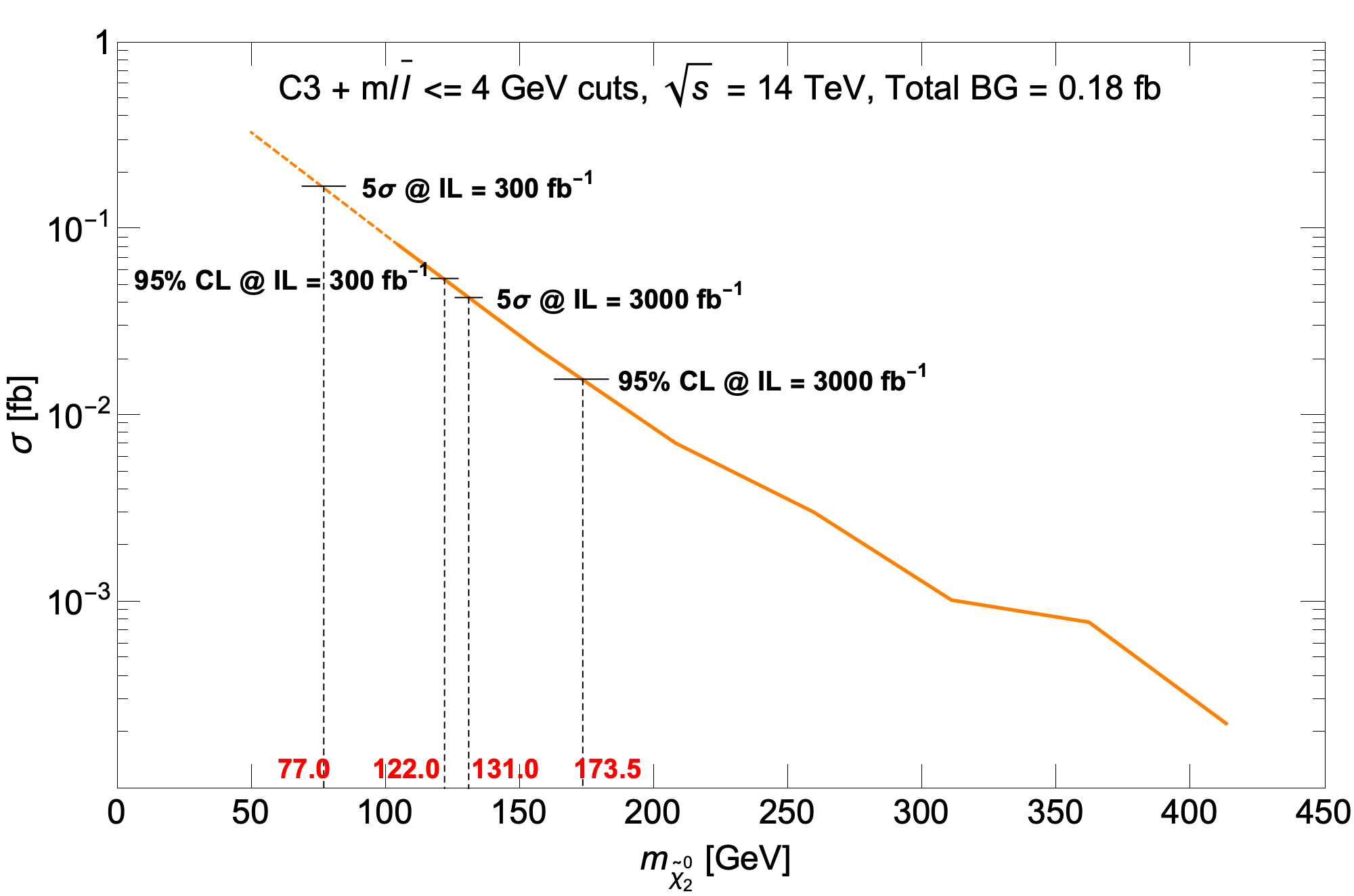
(a)

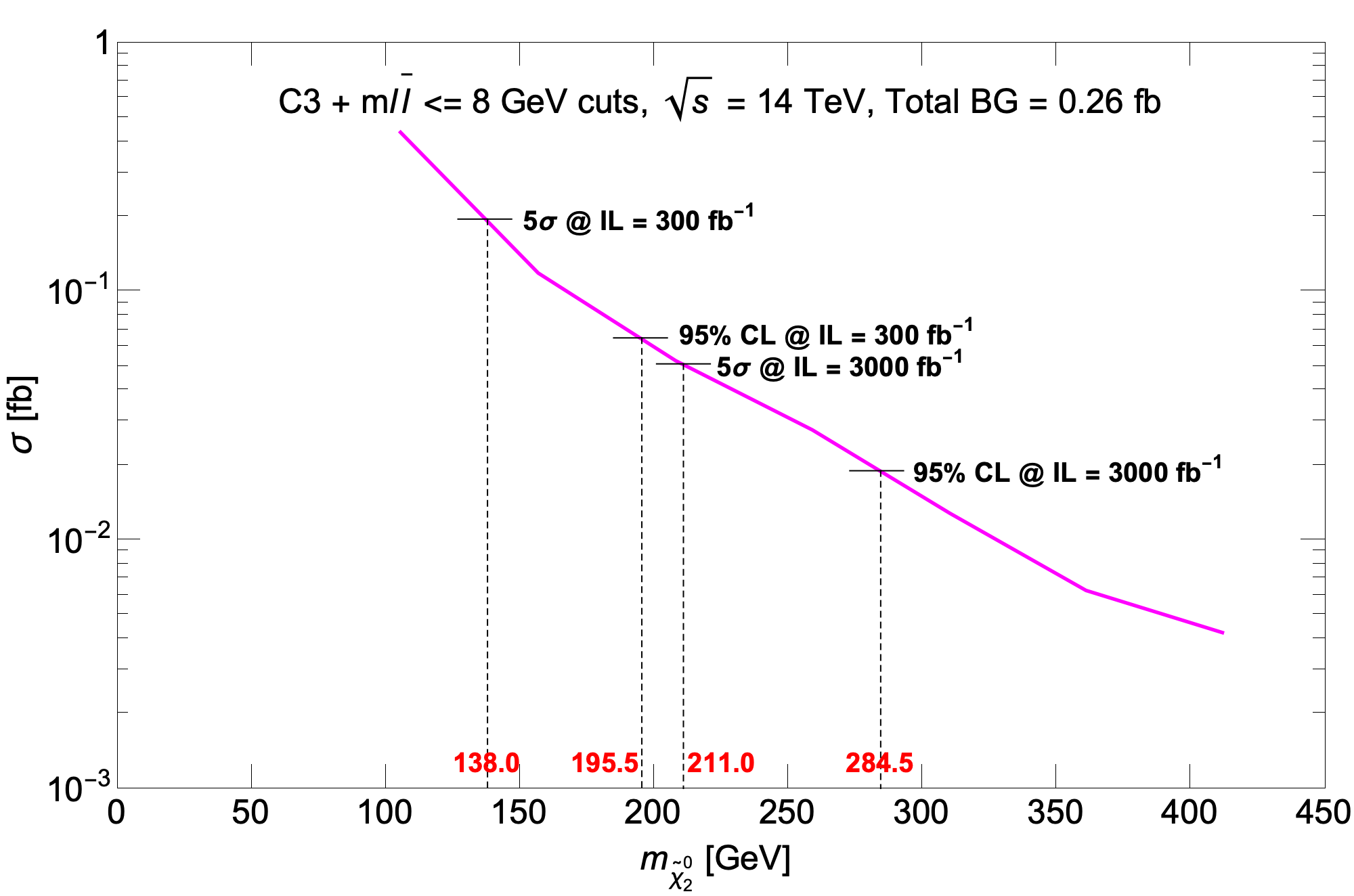
(b)

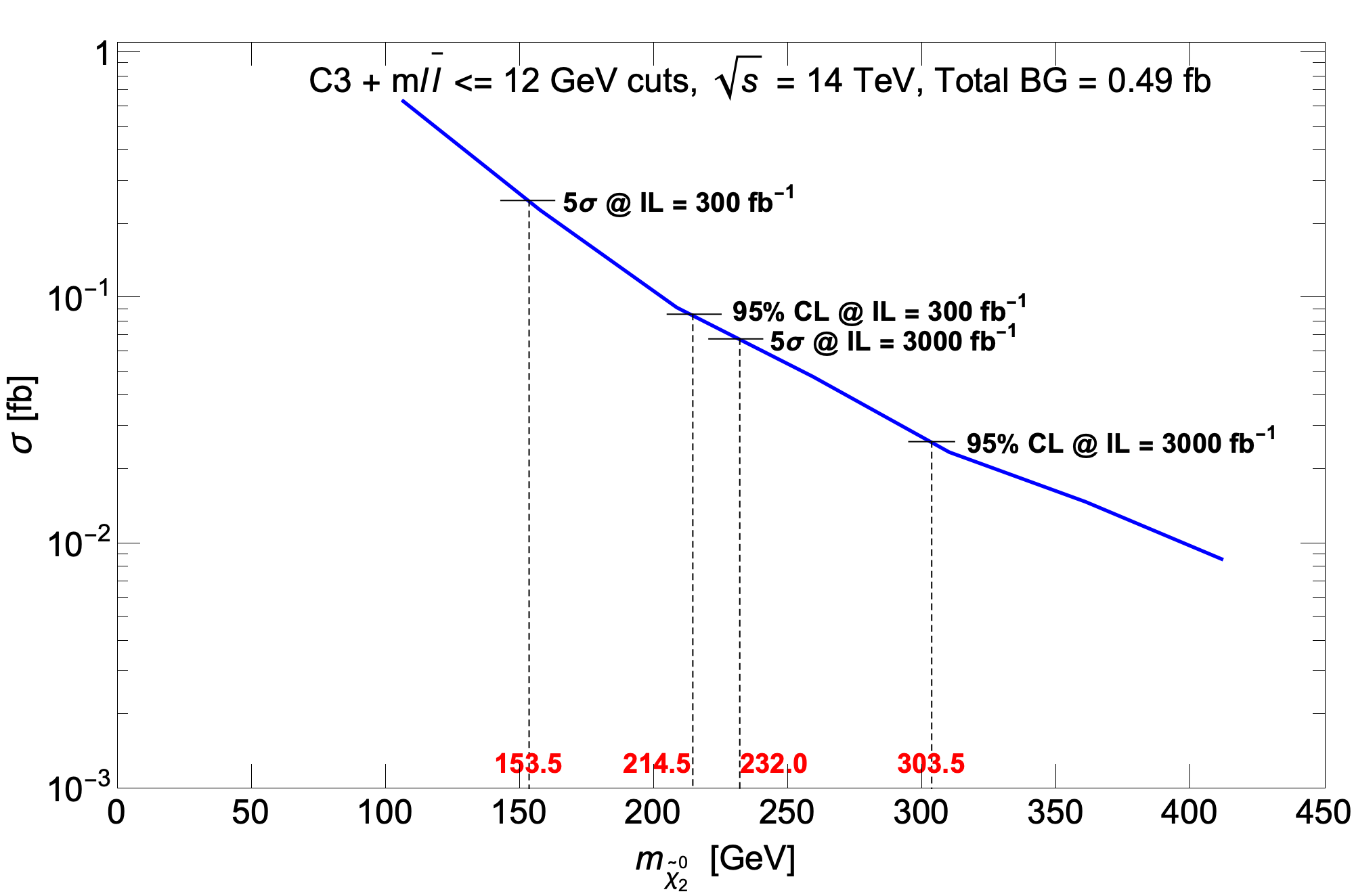
(c)

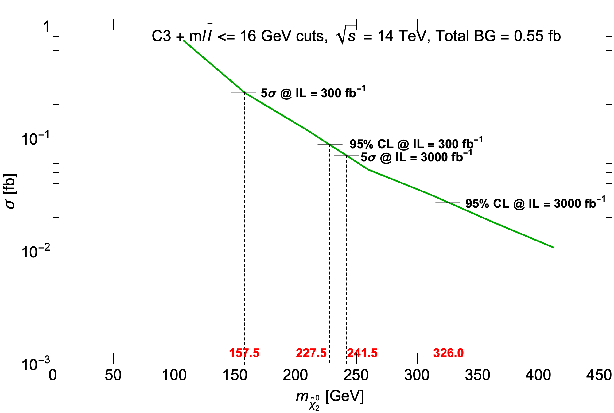
(d)

Figure 20: The projected $5\sigma$ reach and 95% CL exclusion of the HL-LHC with 3000 fb^-1 in $\mu$ for four different NUHM2 model lines with a) $\Delta m=4$ GeV, b) $\Delta m=8$ GeV, c) $\Delta m=12$ GeV and d) $\Delta m=16$ GeV after $C3+m(\ell\bar{\ell})<m_{\widetilde{\chi}^{0}_{2}}-m_{\widetilde{\chi}^{0}_{1}}$ cuts. We also list the total background in each frame in case the reader wishes to estimate the statistical significance of the signal for different choices of integrated luminosity.

In Fig. 21, we translate the results of Fig. 20 into the standard $m_{\widetilde{\chi}^{0}_{2}}$ vs. $\Delta m$ plane. We also show the region excluded by LEP2 chargino searches (gray region). Also shown is current 95%CL exclusion region (labelled ATLAS) along with the projections of what searches at the HL-LHC would probe at the 95%CL [43]: ATLA (soft-lepton A) and CMS (soft-lepton B). We see that the reach that we obtain compares well with the corresponding projections by the ATLAS and CMS collaborations. Our focus here has been on higgsino mass gaps $\lesssim 20-25$ GeV, expected in natural SUSY models. For larger mass gaps, the search strategy explored in this paper becomes less effective because of increased backgrounds from $t\bar{t}$, $WWj$ and other SM processes, and the reach contours begin to turn over. In this case, it may be best to search for higgsinos via the hard multilepton events, without the need for a QCD jet.

Before closing this section, we note that we have only considered physics backgrounds in our analysis. The ATLAS collaboration has, however, reported that a significant portion of the background comes from fake leptons, both $e$ and $\mu$. Accounting for these detector-dependent backgrounds (which may well be sensitive to the HL-LHC environment as well as upgrades to the detectors) require data driven methods which are beyond the scope of our study. We point out, however, that the reader can roughly gauge the impact of the fakes on the contours shown in Fig. 21 using the curves in Fig. 20. For instance, if the fakes increase the background by a factor $f$, the cross section necessary to maintain the same significance for the signal would have to increase by $\sqrt{f}$; i.e. if the fakes doubled the background, for $\Delta m$=8 GeV, the HL-LHC discovery limit would reduce by $\sim 25$ GeV. In the same vein, the reach would be increased by $\sim 30$ GeV if the data from the two experiments could be combined.

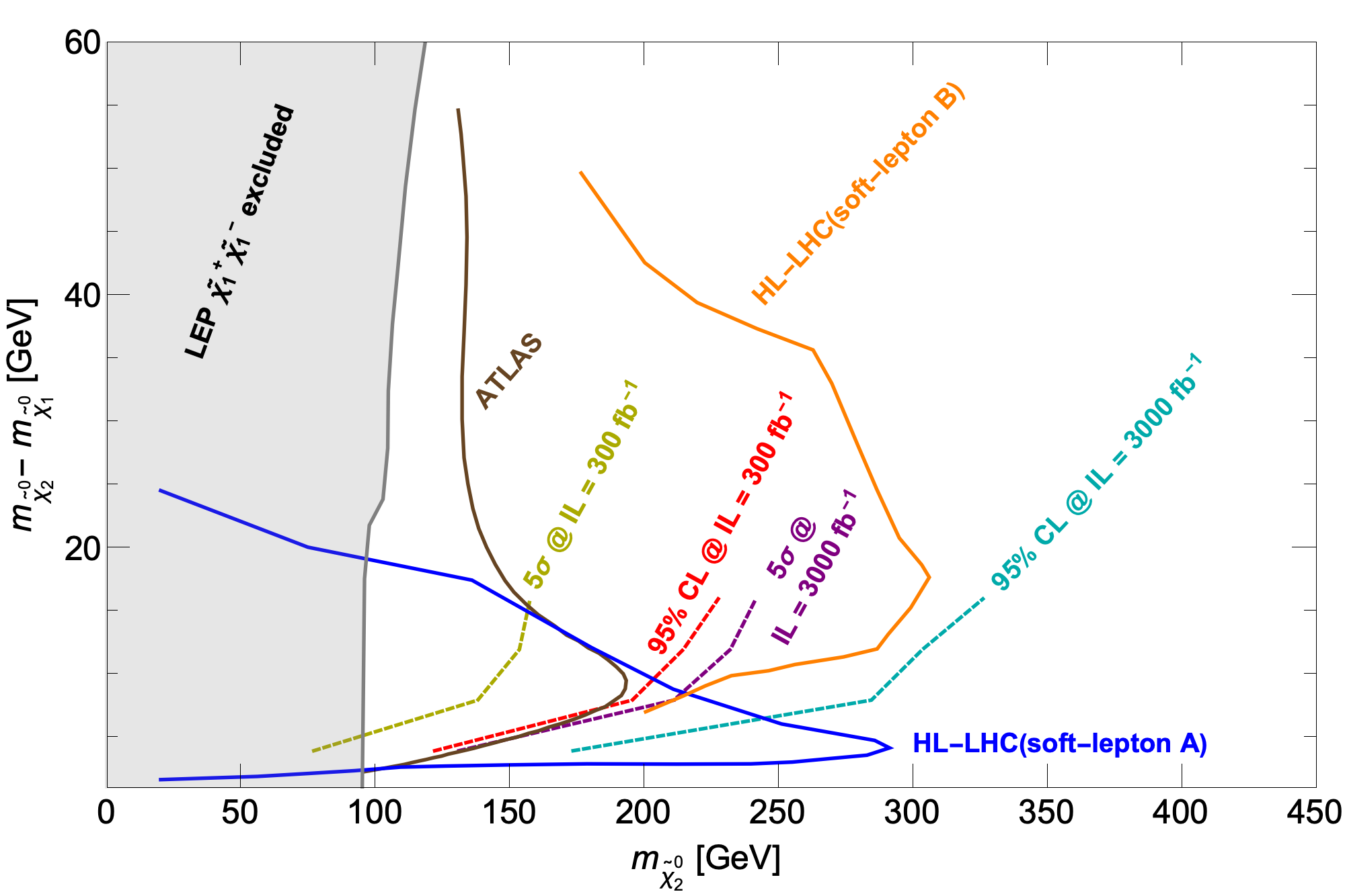
Figure 21: The projected $5\sigma$ reach and 95% CL exclusion contours for LHC14 with 300 and 3000 fb^-1 in the $m_{\widetilde{\chi}^{0}_{2}}$ vs. $\Delta m$ plane after $C4$ cuts. Also shown is the current 95% CL exclusion (ATLAS) and the projected 95% CL exclusions from two different analyses for the HL-LHC [43].

6 Conclusions

It is generally agreed that naturalness in supersymmetric models requires the SUSY preserving higgsino mass $\mu$ rather nearby to the weak scale, because it enters Eq. (1) at tree level. The soft SUSY breaking parameters, however, may be well beyond the TeV scale without compromising naturalness as long as $m_{H_{u}}^{2}$ is driven to small negative values at the weak scale. Indeed, a subset of us [28, 31, 32, 33] have advocated that anthropic considerations on the string landscape favour large values of soft SUSY breaking parameters, but not so large that their contributions to the weak scale are too big. Such a scenario favours $m_{h}\sim 125$ GeV with sparticles other than higgsinos well beyond HL-LHC reach. While stringy naturalness provides strong motivation for higgsino pair production reactions as the most promising avenue to SUSY discovery at LHC14, the phenomenological analysis presented in this paper applies to any MSSM framework with a compressed spectrum of light higgsinos.

We have re-examined the prospects for a search for soft opposite-sign/same flavor dilepton plus $\not\!\!\!{E_{T}}$ from higgsino pair production in association with a hard monojet at LHC with $\sqrt{s}=14$ TeV. The dileptons originate from $\widetilde{\chi}^{0}_{2}\rightarrow\ell\bar{\ell}\widetilde{\chi}^{0}_{1}$ so that the dilepton pair has a distinctive kinematic edge with $m(\ell\bar{\ell})<m_{\widetilde{\chi}^{0}_{2}}-m_{\widetilde{\chi}^{0}_{1}}$, while the monojet serves as the event trigger.

We examined several signal benchmark cases, and compared the signal against SM backgrounds from $t\bar{t}$, $\tau\bar{\tau}j$, $WWj$, $W\ell\bar{\ell}j$ and $Z\ell\bar{\ell}j$ production. The ditau mass reconstruction $m_{\tau\tau}^{2}$, valid in the collinear tau decay approximation for decays of relativistic taus, has been used to reduce the dominant background from $Z(\rightarrow\tau\bar{\tau})+j$ production. However, significant ditau background remains even after the $m_{\tau\tau}^{2}<0$ cut. In this paper, we proposed a new set of angular cuts which eliminate ditau backgrounds much more efficiently at relatively low cost to signal. Additional analysis cuts allow for substantial rejection of $t\bar{t}$ and other SM backgrounds. In the end, we expect higgsino pair production to manifest itself as a low end excess in the $m(\ell\bar{\ell})$ mass distribution with a cutoff at the $\Delta m=m_{\widetilde{\chi}^{0}_{2}}-m_{\widetilde{\chi}^{0}_{1}}$ value, with a tail extending to larger values of $m(\ell\bar{\ell})$ when the two leptons originate in different higgsinos. Using the so-called C3$+m(\ell\bar{\ell})$ cuts, we evaluated the reach of LHC14 for 300 and 3000 fb^-1 of integrated luminosity.

Our final result is shown in Fig. 21. We see that the reach is strongest for larger $\Delta m$ values up to $15-20$ GeV but drops off for smaller mass gaps. Mass gaps smaller than about 4 GeV occur only for very heavy gauginos that fail to satisfy our naturalness criterion, while higgsinos with an uncompressed spectrum would have large mixing with the electroweak gauginos and can be more effectively searched for via other channels. We see from Fig. 21 that the HL-LHC with 3000 fb^-1 gives a $5\sigma$ discovery reach to $m_{\widetilde{\chi}^{0}_{2}}\sim 240$ GeV, with the 95% CL exclusion limit extending to $\sim 325$ GeV for $\Delta m\sim 16$ GeV. Nonetheless, a significant portion of natural parameter space with $\mu\sim m_{\widetilde{\chi}^{0}_{2}}\sim 200-350$ GeV and $\Delta m\sim 4-10$ GeV may still be able to evade HL-LHC detection. Given the importance of this search, we urge our experimental colleagues to see if it is possible to reliably extend the lepton acceptance to yet lower $p_{T}$ values, or increase $b$-quark rejection even beyond 80-85% that has already been achieved.

Acknowledgements:

This work has been performed as part of a contribution to the Snowmass 2022 workshop. This material is based upon work supported by the U.S. Department of Energy, Office of Science, Office of Basic Energy Sciences Energy Frontier Research Centers program under Award Number DE-SC-0009956 and U.S. Department of Energy Grant DE-SC-0017647. The work of DS was supported by the Ministry of Science and Technology (MOST) of Taiwan under Grant No. 110-2811-M-002-574.

References

- [1] G. Aad et al. [ATLAS Collaboration], Phys. Lett. B716 (2012) 1.
- [2] S. Chatrchyan et al. [CMS Collaboration], Phys. Lett. B716 (2012) 30.
- [3] L. Susskind, Phys. Rev. D 20, 2619-2625 (1979) doi:10.1103/PhysRevD.20.2619 .
- [4] M. J. G. Veltman, Acta Phys. Polon. B 12, 437 (1981) Print-80-0851 (MICHIGAN).
- [5] E. Witten, Nucl. Phys. B 188 (1981) 513; R. K. Kaul, Phys. Lett. 109B (1982) 19.
- [6] H. Baer and X. Tata, “Weak scale supersymmetry: From superfields to scattering events,” Cambridge, UK: Univ. Pr. (2006) 537 p.
- [7] A. Canepa, Rev. Phys. 4, 100033 (2019) doi:10.1016/j.revip.2019.100033 .
- [8] M. Aaboud et al. [ATLAS Collaboration], Phys. Rev. D 97 (2018) no.11, 112001 doi:10.1103/PhysRevD.97.112001 [arXiv:1712.02332 [hep-ex]]; T. A. Vami [ATLAS and CMS Collaborations], PoS LHCP 2019 (2019) 168 doi:10.22323/1.350.0168 [arXiv:1909.11753 [hep-ex]].
- [9] The ATLAS collaboration [ATLAS Collaboration], ATLAS-CONF-2019-017; A. M. Sirunyan et al. [CMS Collaboration], arXiv:1912.08887 [hep-ex].
- [10] H. Baer, X. Tata and J. Woodside, Phys. Rev. D 42, 1568-1576 (1990) doi:10.1103/PhysRevD.42.1568 .
- [11] J. R. Ellis, K. Enqvist, D. V. Nanopoulos and F. Zwirner, Mod. Phys. Lett. A 1, 57 (1986).
- [12] R. Barbieri and G. F. Giudice, Nucl. Phys. B 306, 63 (1988).
- [13] S. Dimopoulos and G. F. Giudice, Phys. Lett. B 357 (1995) 573.
- [14] G. W. Anderson and D. J. Castano, Phys. Rev. D 53 (1996) 2403.
- [15] H. Baer, V. Barger and D. Mickelson, Phys. Rev. D 88, 095013 (2013).
- [16] A. Mustafayev and X. Tata, Indian J. Phys. 88 (2014) 991.
- [17] H. Baer, V. Barger, D. Mickelson and M. Padeffke-Kirkland, Phys. Rev. D 89 (2014) no.11, 115019 doi:10.1103/PhysRevD.89.115019 [arXiv:1404.2277 [hep-ph]].
- [18] M. Dine, Ann. Rev. Nucl. Part. Sci. 65, 43-62 (2015) doi:10.1146/annurev-nucl-102014-022053 [arXiv:1501.01035 [hep-ph]].
- [19] H. Baer, V. Barger, P. Huang, A. Mustafayev and X. Tata, Phys. Rev. Lett. 109, 161802 (2012).
- [20] H. Baer, V. Barger, P. Huang, D. Mickelson, A. Mustafayev and X. Tata, Phys. Rev. D 87, 115028 (2013).
- [21] H. Baer, V. Barger and M. Savoy, Phys. Rev. D 93, no.3, 035016 (2016) doi:10.1103/PhysRevD.93.035016 [arXiv:1509.02929 [hep-ph]].
- [22] H. Baer, V. Barger, J. S. Gainer, D. Sengupta, H. Serce and X. Tata, Phys. Rev. D 98, no.7, 075010 (2018) doi:10.1103/PhysRevD.98.075010 [arXiv:1808.04844 [hep-ph]].
- [23] S. Weinberg, Phys. Rev. Lett. 59, 2607 (1987) doi:10.1103/PhysRevLett.59.2607 .
- [24] R. Bousso and J. Polchinski, JHEP 06, 006 (2000) doi:10.1088/1126-6708/2000/06/006 [arXiv:hep-th/0004134 [hep-th]].
- [25] M. R. Douglas, “Statistical analysis of the supersymmetry breaking scale,” hep-th/0405279.
- [26] L. Susskind, “Supersymmetry breaking in the anthropic landscape,” doi:10.1142/9789812775344_0040 [arXiv:hep-th/0405189 [hep-th]].
- [27] N. Arkani-Hamed, S. Dimopoulos and S. Kachru, [arXiv:hep-th/0501082 [hep-th]].
- [28] H. Baer, V. Barger, M. Savoy and H. Serce, Phys. Lett. B 758 (2016), 113-117 doi:10.1016/j.physletb.2016.05.010 [arXiv:1602.07697 [hep-ph]].
- [29] K. J. Bae, H. Baer, V. Barger and D. Sengupta, Phys. Rev. D 99, no.11, 115027 (2019) doi:10.1103/PhysRevD.99.115027 [arXiv:1902.10748 [hep-ph]].
- [30] V. Agrawal, S. M. Barr, J. F. Donoghue and D. Seckel, Phys. Rev. Lett. 80 (1998) 1822 doi:10.1103/PhysRevLett.80.1822 [hep-ph/9801253]; V. Agrawal, S. M. Barr, J. F. Donoghue and D. Seckel, Phys. Rev. D 57 (1998) 5480 doi:10.1103/PhysRevD.57.5480 [hep-ph/9707380].
- [31] H. Baer, V. Barger, H. Serce and K. Sinha, JHEP 03 (2018), 002 doi:10.1007/JHEP03(2018)002 [arXiv:1712.01399 [hep-ph]].
- [32] H. Baer, V. Barger, S. Salam, H. Serce and K. Sinha, JHEP 04 (2019), 043 doi:10.1007/JHEP04(2019)043 [arXiv:1901.11060 [hep-ph]].
- [33] H. Baer, V. Barger and S. Salam, Phys. Rev. Research. 1 (2019), 023001 doi:10.1103/PhysRevResearch.1.023001 [arXiv:1906.07741 [hep-ph]].
- [34] H. Baer, V. Barger, P. Huang, D. Mickelson, A. Mustafayev, W. Sreethawong and X. Tata, JHEP 12, 013 (2013) [erratum: JHEP 06, 053 (2015)] doi:10.1007/JHEP12(2013)013 [arXiv:1310.4858 [hep-ph]].
- [35] H. Baer, V. Barger and P. Huang, JHEP 1111 (2011) 031.
- [36] Z. Han, G. D. Kribs, A. Martin and A. Menon, “Hunting quasidegenerate Higgsinos,” Phys. Rev. D 89 no.7, 075007 (2014); H. Baer, A. Mustafayev and X. Tata, “Monojet plus soft dilepton signal from light higgsino pair production at LHC14,” Phys. Rev. D 90 no.11, 115007 (2014)
- [37] H. Baer, A. Mustafayev and X. Tata, “Monojet plus soft dilepton signal from light higgsino pair production at LHC14,” Phys. Rev. D 90, no.11, 115007 (2014) doi:10.1103/PhysRevD.90.115007 [arXiv:1409.7058 [hep-ph]].
- [38] C. Han, D. Kim, S. Munir and M. Park, “Accessing the core of naturalness, nearly degenerate higgsinos, at the LHC,” JHEP 1504, 132 (2015).a
- [39] M. Aaboud et al. [ATLAS], “Search for electroweak production of supersymmetric states in scenarios with compressed mass spectra at TeV with the ATLAS detector,” Phys. Rev. D 97 (2018) no.5, 052010 doi:10.1103/PhysRevD.97.052010 [arXiv:1712.08119 [hep-ex]].
- [40] G. Aad et al. [ATLAS collaboration], “Searches for electroweak production of supersymmetric particles with compressed mass spectra in 13 TeV collisions with the ATLAS detector,” Phys. Rev. D 101 (2020) no.5, 052005 doi:10.1103/PhysRevD.101.052005 [arXiv:1911.12606 [hep-ex]].
- [41] A. M. Sirunyan et al. [CMS], “Search for new physics in events with two soft oppositely charged leptons and missing transverse momentum in proton-proton collisions at 13 TeV,” Phys. Lett. B 782 (2018), 440-467 doi:10.1016/j.physletb.2018.05.062 [arXiv:1801.01846 [hep-ex]].
- [42] CMS collaboration, “Search for physics beyond the standard model in final states with two or three soft leptons and missing transverse momentum in proton-proton collisions at 13 TeV,” CMS-PAS-SUS-18-004
- [43] A. Canepa, T. Han and X. Wang, doi:10.1146/annurev-nucl-031020-121031 [arXiv:2003.05450 [hep-ph]].
- [44] H. Baer, V. Barger, M. Savoy and X. Tata, Phys. Rev. D 94, no.3, 035025 (2016) doi:10.1103/PhysRevD.94.035025 [arXiv:1604.07438 [hep-ph]].
- [45] H. Baer, V. Barger, S. Salam, D. Sengupta and X. Tata, Phys. Lett. B 810, 135777 (2020) doi:10.1016/j.physletb.2020.135777 [arXiv:2007.09252 [hep-ph]].
- [46] F. E. Paige, S. D. Protopopescu, H. Baer and X. Tata, [arXiv:hep-ph/0312045 [hep-ph]].
- [47] J. Alwall, M. Herquet, F. Maltoni, O. Mattelaer and T. Stelzer, JHEP 06, 128 (2011) doi:10.1007/JHEP06(2011)128 [arXiv:1106.0522 [hep-ph]].
- [48] T. Sjostrand, S. Mrenna and P. Z. Skands, JHEP 05, 026 (2006) doi:10.1088/1126-6708/2006/05/026 [arXiv:hep-ph/0603175 [hep-ph]].
- [49] J. de Favereau et al. [DELPHES 3], JHEP 02, 057 (2014) doi:10.1007/JHEP02(2014)057 [arXiv:1307.6346 [hep-ex]].
- [50] H. Baer, V. Barger, H. Serce and X. Tata, Phys. Rev. D 94, no.11, 115017 (2016) doi:10.1103/PhysRevD.94.115017 [arXiv:1610.06205 [hep-ph]].
- [51] H. Baer, V. Barger, D. Sengupta and X. Tata, Eur. Phys. J. C 78, no.10, 838 (2018) doi:10.1140/epjc/s10052-018-6306-y [arXiv:1803.11210 [hep-ph]].
- [52] M. Cacciari, G. P. Salam and G. Soyez, JHEP 04, 063 (2008) doi:10.1088/1126-6708/2008/04/063 [arXiv:0802.1189 [hep-ph]].
- [53] M. Cacciari, G. P. Salam and G. Soyez, Eur. Phys. J. C 72, 1896 (2012) doi:10.1140/epjc/s10052-012-1896-2 [arXiv:1111.6097 [hep-ph]].
- [54] ATLAS collaboration, ”Expected performance of the ATLAS -tagging algorithms in Run-2”, ATL-PHYS-PUB-2015-022
- [55] H. Baer, V. Barger, D. Sengupta and X. Tata, [arXiv:2203.03700 [hep-ph]].
- [56] H. Baer, V. D. Barger and R. J. N. Phillips, Phys. Rev. D 39, 3310 (1989) doi:10.1103/PhysRevD.39.3310.
- [57] R. Kadala, Ph. D. dissertation, arXiv:1205.1267; R. Kitano and Y. Nomura, Phys. Rev. D 73, 095004 (2006).