MUVINE: Multi-stage Virtual Network Embedding in Cloud Data Centers using Reinforcement Learning based Predictions

Abstract

The recent advances in virtualization technology have enabled the sharing of computing and networking resources of cloud data centers among multiple users. Virtual Network Embedding (VNE) is highly important and is an integral part of the cloud resource management. The lack of historical knowledge on cloud functioning and inability to foresee the future resource demand are two fundamental shortcomings of the traditional VNE approaches. The consequence of those shortcomings is the inefficient embedding of virtual resources on Substrate Nodes (SNs). On the contrary, application of Artificial Intelligence (AI) in VNE is still in the premature stage and needs further investigation. Considering the underlying complexity of VNE that includes numerous parameters, intelligent solutions are required to utilize the cloud resources efficiently via careful selection of appropriate SNs for the VNE. In this paper, Reinforcement Learning based prediction model is designed for the efficient Multi-stage Virtual Network Embedding (MUVINE) among the cloud data centers. The proposed MUVINE scheme is extensively simulated and evaluated against the recent state-of-the-art schemes. The simulation outcomes show that the proposed MUVINE scheme consistently outperforms over the existing schemes and provides the promising results.

I Introduction

The cloud computing is a recent advancement in virtualization technology that can dynamically provision infinite computing resources to the end users on pay as you use basis. The primary concern of any Cloud Service Provider (CSP) is to ensure the quality of cloud services to the end users with optimum computing resources that translate into the maximum profit. Accordingly, various heuristics-based, nature-inspired learning-based, and Artificial Intelligence (AI) based approaches are proposed for the efficient cloud resource management. The AI is one of the promising alternatives that potentially aid in efficient cloud resource management. AI is known as the machine demonstrated intelligence and it is considered as a group of techniques designed to tackle the application-specific problems such as prediction, classification, recognition, visualization etc. Prominent AI techniques such as Fuzzy Logic, Machine Learning (ML) and Deep Learning (DL) exist to deal with various problems in every walk of our life. Among them, ML is typically used to process the text and numeric dataset. Generally, ML techniques are broadly classified into three categories such as supervised, unsupervised, and reinforcement learning with primary objective to let the machine extract, analyze, train, and build the prediction models on the top of the training dataset. In supervised learning, machine learns from the supplied labels often called as the observed true outcomes; whereas, in unsupervised learning, the machine learns without the known outcomes. Contrary to the supervised and unsupervised learning, the agent (machine) learns in real-time from the environment to optimize the given problem in reinforcement learning.

Although AI techniques help to build an efficient prediction model, it poses numerous challenges as well. The foremost challenge is to choose the right AI technique for a given application, dataset type, size, and nature of the problem. However, considering the robustness, the recent years have witnessed a myriad growth of applications of AI gradually replacing the traditional approaches with improved accuracy. The home automation [1], self-driving car [2], cardiac signal processing [3], automated cloud resource management [4] are considered few of the potential applications that benefit the most by AI. Among the aforementioned applications, automated cloud resource management is considered as the challenging one due to the underlying complexity.

On the other hand, cloud computing environment provides the computing and storage resources to the users, which encourages the users to execute the complex applications and stores the raw data without concerning much about the storage space [5]. The computing and storage as virtual resources are provision to the end users by implementing the virtualization technology atop the substrate resources [6]. Different service models are used to provide the virtual resources such as the Infrastructure as a Service (IaaS), Software as a Service (SaaS) etc. In order to access the resources using IaaS model, users need to send the request in the form of Virtual Network (VN). Typically, each VN request may comprised of a number of Virtual Machines (VMs) with the corresponding resource configuration, and the network topology that defines the communication among the VMs [7].

On receiving the VN request, CSP creates the required VMs onto a set of suitably interconnected Substrate Nodes (SNs) and establishes the communication links among the VMs. The aforementioned process is called as a Virtual Network Embedding (VNE). In general, VNE refers to the embedding of the VMs and virtual links in a sequential or parallel manner. However, the SN utilization is one of the major research issues that needs to be addressed while embedding the VN. In the past decade, different approaches are followed to efficiently carry out the VNE process. In [7], graph theory is used as a tool for the VNE. In [7], the VN request and the substrate network are treaterd as graphs and the sub-graph from the substrate network equivalent to that of the VN request is obtained. In [8], Hidden Markov Model is used to model the VNE problem. Ant colony optimization [9] and Particle swarm optimization [10] are few of the machine learning methods that are applied in the VNE process.

The machine learning approaches may use the historical information of the incoming VN request, substrate network, and the usage history. The VN request may includes the resource demand of VMs. Each VM is further associated with the priority value decided in accordance with the Service Level Agreement (SLA), which indicates the importance of the corresponding VM in resource allocation process. Upon embedding the VN onto the SNs, the actual resource usage information is obtained. On the other hand, historical information regarding the SNs includes the amount of the resources allocated to the VN request, actual resource usage by the VMs, throughput of each SN, addition and removal of the SNs at different time stamps. It is assumed that the CSP is empowered with different software tools to collect such historical information [11]. The historical information also includes the type of VN requests accepted and rejected under different cloud scenarios. Further, such labelled data are useful in the embedding process to provision the suitable SNs for each VN request type. The supervised ML algorithms such as linear regression, support vector machine and Naive Bayes can be considered as the suitable alternatives for the aforementioned data. However, it is essential to design the ML algorithms, which explore the cloud environment and exploit the VM placement strategies for the real-time embedding of VMs on SNs.

I-A Motivation

The substrate resource utilization plays a major role in embedding the VNs as it has the direct impact on the acceptance ratio and revenue of the CSP. Here, the substrate resource refers to as the CPU, memory, and network. The utilization refers to as the percentage of the resources utilized by the VMs out of the allocated. Usually, the exact amount of resources is allocated to VMs and the virtual links to fulfill the resource demand of the requested VNs. However, our analysis of the historical dataset [11] reveals that resources normally stay underutilized leading to the overall ineffective resource utilization.

Furthermore, the workload distribution of substrate resources to VNs plays an important part in cloud resource management. Normally, it is preferable to have uniform substrate resource allocation to VNs across the cloud. Fig. 1 illustrates the possible problem scenario that may arise under the uneven workload distribution. Let CSP is comprised of $SN_{1}$ and $SN_{2}$ with maximum CPU capacity of $14$ and $12$ units, respectively and the maximum memory capacity of $150$ units each, as shown in Fig. 1(a). Let CSP receives VN requests $VN_{1},VN_{2},VN_{3},$ and $VN_{4}$ with the CPU demand of $5$, $3$, $5$, and $2$ units, respectively and memory demand of $20$, $65$, $13$, and $83$ units, respectively as shown in Fig. 1(a). The CSP may embed VN requests in two different ways depicted as Uneven distribution and Even distribution as shown in Fig. 1(c). In case of Uneven distribution, CSP ends up allocating $71.4\%$ and $41.6\%$ units of the CPU resources, and $22\%$ and $98.6\%$ units of the memory resources of $SN_{1}$ and $SN_{2}$, respectively as shown in Fig. 1(c). However, in Even distribution, the resources are evenly distributed among the SNs. The benefit of Even distribution can be realized as shown in Fig. 1(d). On the arrival of new virtual network request $VN_{5}$ with CPU and memory demand of $5$ and $36$ units, respectively as shown in Fig. 1(b), it becomes infeasible to embed the $VN_{5}$ in case of Uneven distribution. On the contrary, $VN_{5}$ can be successfully embedded onto $SN_{1}$ or $SN_{2}$ in case of Even distribution as shown in Fig. 1(d).

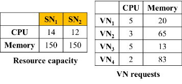
(a) VN requests and resource capacity of $SN_{1}$ and $SN_{2}$.

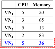
(b) A new VN request $VN_{5}$.

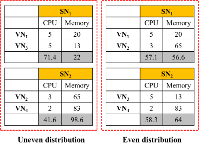
(c) Two possible solutions, Uneven distribution and Even distribution.

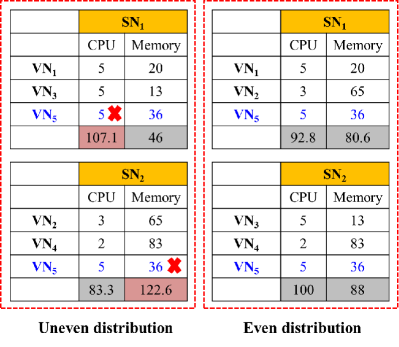
(d) Embedding new $VN_{5}$ in Uneven distribution and Even distribution.

Figure 1: A motivational example on computing resource utilization.

It is assumed that at any given time, substrate node can host multiple VMs of a VN. Under such circumstances, the VN can be treated as a small graph upon embedding where each vertex would represent the group of VMs hosted on each SN, and the new virtual link represents the link between the corresponding SNs. The advantage of such embedding solution is that the network resource demand among VMs in the same substrate node can be ignored as no physical link is involved. However, the computing resources consumed for the communication between the VMs on same SN are not ignored. It is necessary to distribute the VMs of a VN in such a way that the new network resource demand of the virtual links can be minimized. Considering the aforementioned research issues, our goals can be summarized as to design a reinforcement learning based prediction models for multi-stage virtual network embedding in cloud data center to identify and allocate the suitable substrate nodes to VN requests for subsequent improvement in the overall resource utilization.

The rest of the paper is organized as follows. Section II describes the related works and the problem is formulated in Section III. The Multi-stage Virtual Network Embedding (MUVINE) scheme is described in Section IV followed by the knowledge-based AI models in Section V. The simulation setup and corresponding results are presented in Section VI and concluding remarks are made in Section VII.

II Related Works

In the recent past, a number of VNE schemes have been proposed considering Data Center (DC) network topologies [12], resource utilization [13], energy consumption [14], revenue and profit [15, 16], and survivability of VN [17]. A brief summary of the resource allocation schemes is presented in [18]. The VNE schemes are structured in three broad categories such as Heuristic-based, Nature-inspired learning-based, and Reinforcement learning-based as discussed below.

II-A Heuristic-based

The minimization of a total number of required SNs subsequently improves the overall computing resource utilization. In [7], a link-based virtual resource management algorithm is proposed considering the substrate network parameters such as the load, round trip time, and energy consumption. However, it is observed that resource utilization can be optimized further by analyzing the historical virtual network requests including the actual resource usage, substrate resource availability, etc. In [13], the degree of the nodes and their cluster coefficient are used to find out the importance of the respective node and thereby to find out the set of suitable substrate nodes to embed the VN requests. Although the network topology is taken into consideration for the VNE, the dependencies among the VNs are not considered. This results in inefficient VNE in terms of resource utilization. In [19], multiple VM clusters are mapped in a federated cloud environment. The goal of the [19] is to minimize the network latency with maximization of acceptance ratio. However, authors in [19] overlook the fact that geographically distributed cloud environment incurs the extra cost in terms of time. In [20], location preference of the users is considered to design the VNE algorithm. The VNE problem is formulated as a graph bisection problem, and VMs and the virtual links are mapped in an integrated manner. In order to reduce the substrate server failure impact, VMs are mapped onto separate substrate servers. However, such mapping results in inefficient network resource utilization.

To provide full network bandwidth guarantee in case of multiple substrate network failure is a challenging issue in cloud management. In [17], a survivable VNE algorithm is proposed by formulating the optimal solution as a quadratic integer program. However, the VNE scheme [17] often requires network bandwidth in excess to that of the actual demand. The excess resource requirement can further be minimized by analyzing the actual network resource requirement, which can be predicted by investigating the historical information. In [21], an I-VNE algorithm is proposed considering the link interference. The I-VNE algorithm embeds the VNs by considering the temporal and the spatial network topology. The primary advantage of I-VNE algorithm is VNs are embedded with low interference. In [15], a Multi-commodity flow and shortest-path approaches are followed to embed VNs onto SNs with the objective to maximize the profit of infrastructure provider. The proposed scheme [15] maps the VMs and the virtual links without splitting the substrate path. However, future resource demand and historical information are not considered, which restricts the profit maximization up to certain extent. In [16], a policy-based VNE architecture is proposed that follows network utility maximization approach and separates the high-level goals from the mapping mechanisms of VM and virtual links.

II-B Nature-inspired learning-based

The non-deterministic polynomial hard (NP-hard) characteristic of a VNE problem has encouraged several researchers to explore the nature-inspired learning-based algorithm. In [22], a divide-and-conquer evolutionary algorithm (ODEA) is designed for a large-scale VNE. Large VNs are decomposed into overlapping sub-VNs followed by optimization of each sub-VN using the sub-graph mapping procedure. The decomposition of large VNs into sub-VNs makes the ODEA scalable. However, it likely increases the network complexity of the VNE solution, when multiple sub-VNs are embedded on SNs across the network. Besides, the integration of sub-VNs is also a challenging task and it further complicates the VNE solution.

In [10], a constructive particle swarm optimizer is designed for the VNE (CPSO-VNE). In CPSO-VNE, the VNE process carried out in a step-by-step mapping of each node along with its adjacent virtual links. The CPSO-VNE uses adjacency information to closely embed the virtual nodes in SN topology. However, CPSO-VNE still uses the heuristic information to guide the path information and search. In [23], a distributed VNE system is designed with historical information and meta-heuristic approaches. The particle swarm optimization technique is used to improve the VNE optimization capacity. However, the VNE scheme [23] fails to survive the physical failures such as node or link failure. In [9], a multi-objective ant colony system (MOACS) algorithm is proposed for VM placement in the cloud. The MOACS obtains a set of non-dominated solutions that simultaneously minimize total resource wastage and power consumption.

II-C Reinforcement learning-based

More recently, Reinforcement Learning (RL) based VNE is explored. In [24], RL-based VNE algorithm is proposed considering the historical data of the virtual network requests. However, only the resource capacity is considered as a prominent feature for the analysis, which does not ensure state-of-the-art improvement in results. In addition to the resource capacity, features such as VNs arrival time, execution time, resource demand, and the actual resource usage play critical role in deciding the efficient VNE solution. In [5], the RL-based framework is designed for adaptive resource allocation and provisioning in multi-service cloud environment. The RL-based framework [5] adapts to the system changes such as service cost, resource capacity, and resource demand and it performs well in a multi-service cloud environment. However, it specifically focuses on resource provisioning to satisfy the service level agreement (SLA) of multiple clients.

Considering the underlying complexity of the cloud environment, it is required to embed intelligence to predict the consequences for the smooth functioning of cloud operations. In [25], an intelligent cloud resource management architecture is designed using deep reinforcement learning. The very purpose of the proposed cloud resource management architecture is to enable cloud to efficiently and automatically negotiate the most suitable configuration derived from the underlying complexity. In [26], a coordinated two-stages VNE algorithm is designed using the RL. A pointer network is used to find a node mapping policy and shortest path algorithm is used to embed the links. The VNE algorithm of [26] mainly focuses on the CPU and bandwidth as resources to optimize. However, it is challenging to design an efficient VNE algorithm without considering the memory as a resource. In [27], historical network request data and policy-based RL is designed for node mapping. The overall objective of policy-based RL [27] is to maximize the revenue by embedding nodes and links using convolutional neural network. Similarly, in [28], a deep learning model is designed to predict the cloud workload for the industry informatics. The workflow schedule is an integral operation of any cloud computing environment. The primary objective of workflow scheduling is to optimize the processing cost and thereby enable the cloud to efficiently provide the services to the end-user and at the same time remain profitable. In [29], a Bat Algorithm is employed to efficiently schedule the data-intensive workflow applications. Similarly, the self-management of cloud resources is an important yet challenging objective and needs further investigation. In [4], a dynamic, decentralized, and coordinated neuro-fuzzy approach is proposed to self-manage the substrate network resources.

III Problem Formulation

In this section, the mathematical formulation of the substrate network and virtual network requests is presented. The brief summary of notations used in the paper is presented in Table I.

III-A Substrate network

The typical cloud environment is comprised of a large number of SNs often referred to as the physical machines. It is assumed the SNs are connected through a switch-centric network topology. The resources are divided into two categories such as computing and network. The computing resource refers to CPU and memory. The network of SNs is denoted by $G^{s}(N^{s},E^{s})$, where $N^{s}=\{S_{1},S_{2},S_{3},...,S_{m}\}$ be the set of $m$ SNs, and $E^{s}$ be the set of the substrate links. Each SN is denoted as $S_{i}\in N^{s},1\leq i\leq m$. The maximum computing resource capacity of type $x\in\{CPU,memory\}$ available at each $S_{i}$ is denoted by $C_{i}^{x}$; whereas the remaining computing resource availability is denoted as $A_{i}^{x}$. For example, $A_{5}^{CPU}$ indicates the remaining CPU resource availability of the SN $S_{5}\in N^{s}$. Similarly, $L_{ij}^{a}$ be the network bandwidth availability of substrate link between $S_{i}$ and $S_{j}$. Using the $L_{ij}^{a}$, the network bandwidth availability of the SN $S_{i}$ denoted as $L_{i}^{a}$ can be calculated as follows.

$$L_{i}^{a}=\max_{\forall S_{j}\in N^{s}}\{L_{ij}^{a}\},\quad i\neq j$$ (1)

It is assumed that the SNs may be equipped with different amount of resources. Hence, the $C_{i}^{x}$ and $A_{j}^{x}$ may differ for any substrate nodes $S_{i}$ and $S_{j}$, $i\neq j$. Let $L_{ij}^{l}$ be the total number of physical links in the shortest path between $S_{i}$ and $S_{j}$. A shortest path algorithm, such as Dijkstra’s algorithm, can be used to find the shortest path with minimum number of intermediate physical links.

TABLE I: List of notations

Notation	Description
$G^{s}(N^{s},E^{s})$	Substrate network graph
$N^{s}$	Set of SNs
$E^{s}$	Set of substrate links
$G^{v}(N^{v},E^{v})$	Virtual network graph
$N^{v}$	Set of VMs
$E^{v}$	Set of virtual links
$n$	Total number of VMs in the current VN
$m$	Total number of SNs
$S_{i}$	Represents an SN, $1\leq i\leq m$
$V_{j}$	Represents a VM, $1\leq j\leq n$
$C_{i}^{x}$	Maximum available resource of type $x$ at $S_{i}$, $x\in\{CPU,memory\}$
$A_{i}^{x}$	Amount of resource of type $x$ available at $S_{i}$, $x\in\{CPU,memory\}$
$D_{j}^{x}$	Resource demand of type $x$ by $V_{j}$, $x\in\{CPU,memory\}$
$L_{ij}^{a}$	Amount of network resource available between $S_{i}$ and $S_{j}$
$L_{ij}^{d}$	Network resource demand by the virtual link between $V_{i}$ and $V_{j}$
$L_{ij}^{l}$	The total number of physical links in the shortest path between SN $S_{i}$ and $S_{j}$
$L_{i}^{a}$	Amount of network resource available at $S_{i}$
$L_{j}^{d}$	Network resource demand by $V_{j}$
$\alpha_{j}$	Class of $V_{j}$
$\alpha$	Class of VN request
$\beta$	Priority value of VN request
$\kappa_{i}^{j}$	Boolean value to indicate $V_{j}$ assigned to $S_{i}$
$\omega_{n}$	Resource preference constant
$\phi_{j}$	Start time of $V_{j}$
$\chi_{j}$	End time of $V_{j}$
$rC_{i}^{x}$	Actual resource consumption of type $x$ by $V_{j}$
$\Phi$	Aggregate CPU demand of $G^{v}(N^{v},E^{v})$
$\Psi$	Aggregate memory demand of $G^{v}(N^{v},E^{v})$
$\phi_{v}$	Start time of $G^{v}(N^{v},E^{v})$
$\chi_{v}$	End time of $G^{v}(N^{v},E^{v})$
$rC_{v}^{x}$	Actual resource consumption of type $x$ by $G^{v}(N^{v},E^{v})$
$\ell$	Binary label of VN training dataset
$\zeta$	Number of features in VN dataset
$Q(s_{t},a_{t})$	State-action value function
$\mathbb{R}(G^{v}(N^{v},E^{v}))$	Reward of $G^{v}(N^{v},E^{v})$
$\mathbb{H}$	Decision variable

III-B Virtual network

It is assumed that the cloud users send the request in the form of a virtual network (VN) represented as an undirected weighted graph denoted as $G^{v}(N^{v},E^{v})$. Each $G^{v}(N^{v},E^{v})$ is comprised of a set of $n$ number of VMs denoted as $N^{v}=\{V_{1},V_{2},V_{3},....,V_{n}\}$ and a set of virtual links $E^{v}$. Each VM, denoted by $V_{j},1\leq j\leq n$, is associated with computing resource demand parameter denoted by $D^{x}_{j}$. Here, $x\in\{CPU,memory\}$ represents the computing resource type. Similar to the VM resource demand, each virtual link between VM $V_{i}$ and $V_{j}$ is associated with network bandwidth demand denoted by $L_{ij}^{d}$. Based on the value of $L_{ij}^{d}$, the network bandwidth demand of a particular VM $V_{i}$ can be calculated as follows:

$$L_{i}^{d}=\sum_{\forall V_{j}\in N^{v}}{L_{ij}^{d}}$$ (2)

Let $L_{ij}^{l}(L_{u_{1}u_{2}}^{d})$ be the number of physical links in the shortest path between SN $S_{i}$ and $S_{j}$ provided that this shortest path fulfills the bandwidth demand of virtual link between virtual node $V_{u_{1}}$ and $V_{u_{2}}$. The VNs are assumed to be static in nature. This infers that the resource demand and the structure of the VNs do not change upon the embedding. The end time of the virtual network is unknown. Hence CSP has no information regarding the time duration the computing and network resources need to be reserved for each VN. The boolean variable $\kappa_{i}^{j}$ is used to indicate if $V_{j}$ is assigned to substrate node $S_{i}$. Mathematically,

$$\kappa_{i}^{j}=\left\{\begin{array}[]{c l}1&\text{if }V_{j}~{}\text{is assigned to substrate node }S_{i}\\ 0&\text{Otherwise}\end{array}\right.$$ (3)

III-C VN classes and priority

The incoming requests are classified into three different classes based on the delay sensitiveness: Class 1, Class 2, and Class 3. The class $\alpha_{j},1\leq j\leq n$ of any $V_{j}$ is decided by the user, whereas the class $\alpha$ of any $G^{v}(N^{v},E^{v})$ is decided by the CSP based on the classes of each $V_{j}\in G^{v}(N^{v},E^{v})$. VMs in Class 1, Class 2, and Class 3 are said to be highly, moderately, and less delay sensitive, respectively. CSP strictly follows the resource demand of VMs in Class 1; whereas it is not mandatory for the CSP to strictly fulfill the resource demand of the VMs in Class 3.

Based on the value of $\alpha$, the priority of the VN is derived, which is denoted by $\beta$. Mathematically,

$$\beta=\left\{\begin{array}[]{c l}1&\text{if }\alpha=\emph{Class 3},\text{ less delay sensitive VN}\\ 2&\text{if }\alpha=\emph{Class 2},\text{ mderately delay sensitive VN}\\ 3&\text{if }\alpha=\emph{Class 1},\text{ highly delay sensitive VN}\\ \end{array}\right.$$ (4)

During the substrate resource allocation, VNs with higher priority value such as $\beta=3$, are given higher preference. On the contrary, VNs with less priority value are given less importance in the resource allocation process.

III-D Objective function

Considering the above scenario, the main objective of our proposed MUVINE scheme is to maximize the mean percentage of the resource utilization based on the predictions through the reinforcement learning. The resource maximization must be done along with the maximization of the acceptance rate. Here, the acceptance rate refers to as the percentage of the VNs that are accepted without violating the SLA and resource demands out of the total requested VNs. Mathematically, the objective function can be written as shown in Eq. III-D.

$$maximize~{}Z= \left[\sum_{\forall x\in\{CPU,memory\}}\sum_{\forall S_{i}\in N^{s}}\sum_{\forall V_{j}\in N^{v}}\frac{\kappa_{i}^{j}}{m}*\right.$$

$$\left.\qquad\left(\omega_{x}*{\frac{C_{i}^{x}-A_{i}^{x}+D_{j}^{x}}{C_{i}^{x}}}\right)\right]$$

$$+\left[\sum_{\forall S_{i_{1}},S_{i_{2}}\in N^{s}}\sum_{\forall V_{u_{1}},V_{u_{2}}\in N^{v}}\frac{\omega_{n}*\kappa_{i_{1}}^{u_{1}}*\kappa_{i_{2}}^{u_{2}}}{L_{i_{1}i_{2}}^{l}(L^{d}_{u_{1}u_{2}})}\right]$$ (5)

Constraints:

$$\sum_{i=1}^{m}\kappa_{i}^{j}=1,\quad\forall V_{j}\in N^{v}$$ (6)

$$\forall S_{i}\in N^{s},\nexists V_{j}\in N^{v},D_{j}^{x}\geq A_{i}^{x},L_{j}^{d}\geq L_{i}^{a},x\in\{CPU,memory\}$$ (7)

$$\text{if}~{}\kappa_{i}^{j}=1,\quad 0<D_{j}^{x}<A_{i}^{x}\text{ and }0<L_{j}^{d}<L_{i}^{a}$$ (8)

$$\omega_{n}+\sum_{x\in\{CPU,memory\}}\omega_{x}=1$$ (9)

The objective function shown in Eq. III-D is of two folds, where the first part primarily focuses on maximization of server resources (CPU, memory) utilization and the second part focuses on minimizing the number of physical links used. To minimize the number of physical links, it is encouraged to embed the VMs on the nearby SNs. For this, the Dijkstra algorithm is used to find the shortest path between two SNs. By minimizing the number of physical links, a small amount of network resource is saved for each VN request, which helps increasing the acceptance rate. The obtained solution of the above objective function must satisfy the constraints as shown in Eq. 6 - 9. The constraints are described as follows.

• The constraint shown in Eq. 6 ensures each VM is embedded exactly onto one SN. This implies that no splitting will be done with the VM. Further, it does not guarantee how many number of VMs from one VN request will be embedded onto a single SN.

• The constraint shown in Eq. 7 ensures that VN request is not comprised of any VM with the resource demand greater than the resource availability on any of the SN. To be specific, there exists at least one SN for each VM that fulfills the resource demand.

• The constraint shown in Eq. 8 refers to embedding the VM onto the SN where the resource demand is less than the resource availability, which also indicates that a positive resource demand value is associated with all VMs and virtual links.

• $\omega_{x}$ and $\omega_{n}$ are the constants introduced to assign a preference value to different types of resources such as CPU, memory, and network bandwidth. Constraint as shown in Eq. 9 ensures that the sum of all the constants is $1$.

IV The Multi-stage Virtual Network Embedding (MUVINE) scheme

In this section, the MUVINE scheme is described, which is designed on the top of the reinforcement learning based predictions. It is assumed that the CSP (agent) learns by exploring the existing resources of the cloud data centers (environment). The purpose of exploration is to learn series of actions from the cloud environmental and ascertain an optimum action that maximizes the total cumulative reward of the CSP. The typical cloud environment dataset is described in detail as follow.

IV-A Cloud environment dataset

Let $m$ be the number of SNs with heterogeneous computation and network capacity in a cloud data center. Let multiple applications arrive at the CSP in the form of VNs, which in turn be represented as the set of interconnected VMs. It is to be noted that each VN may have different graph structure and two VNs with the same graph structure may have VMs with different resource requirement. The historical information is comprised of the set of features and labels. The features represent the parameters of VNs, VMs, and SNs.

IV-A1 VM feature set

Let $G^{v}(N^{v},E^{v})$ is comprised of $n$ VMs. Without losing the generality, Let $V_{j}\in G^{v}(N^{v},E^{v})$ contains set of user-specific computational capacity parameters such as CPU and memory demand of the $V_{j}$ represented as $D_{j}^{CPU}$ and $D_{j}^{memory}$, respectively. Besides, each $V_{j}\in G^{v}(N^{v},E^{v})$ also contains the user-specific parameters such as class of the $V_{j}$, priority of $V_{j}$ represented as $\alpha_{j}$ and $\beta_{j}$, respectively. In addition to the user-specific parameters, CSP also records parameters such as start time of $V_{j}$ represented as $\phi_{j}$, end time of $V_{j}$ represented as $\chi_{j}$, actual resource consumption of type $x$ by $V_{j}$ represented as $rC_{j}^{x}$, where $x\in\{CPU,Memory\}$.

IV-A2 VN feature set

Similar to $V_{j}$, the $G^{v}(N^{v},E^{v})$ is also associated with user-specific parameters and CSP recorded parameters. The user-specific parameters associated with $G^{v}(N^{v},E^{v})$ are aggregate CPU demand represented as $\Phi$, aggregate memory demand represented as $\Psi$, class of $G^{v}(N^{v},E^{v})$ represented as $\alpha$, priority of $G^{v}(N^{v},E^{v})$ represented as $\beta$. The CSP recorded parameters associated with VN $G^{v}(N^{v},E^{v})$ are start time of $G^{v}(N^{v},E^{v})$ represented as $\phi_{v}$, end time of $G^{v}(N^{v},E^{v})$ represented as $\chi_{v}$, actual resource consumption of type $x$ by VN $G^{v}(N^{v},E^{v})$ represented as $rC_{v}^{x}$, where $x\in\{CPU,Memory\}$.

IV-A3 SN feature set

At any given time in the cloud, the SNs represented as $S_{i}$, $1\leq i\leq m$ may contain available resource of type $x$ represented as $A_{i}^{x}$, where $x\in\{CPU,memory,network\}$. Moreover, the CSP also records and maintain the available clock rate represented as $A_{i}^{Cr}$.

The aforementioned set of parameters are referred to as the aggregate set of features recorded by CSP for each VN execution and together constitute it as a historical dataset.

IV-B Multi-stage prediction architecture

The multi-stage prediction architecture for VNE is presented in Fig. 2. A binary ML classifier followed by Maximum Likelihood Classifier (MLC) and iterative reinforcement learning are employed to select the set of most appropriate SNs to embed the VN requests. The prediction architecture can be described as follows.

In the first stage, the acceptability of the VN request into the cloud data center is evaluated. A binary ML classifier is designed to classify VN requests into ”accepted” or ”rejected”. The binary classifier is built and trained on the top of the historical dataset of VNs comprised of features as described in Section IV-A2 and an observed binary value of label $\ell\in\{accepted,rejected\}$. It is to note that the label $\ell$ is CSP assigned and it is based on the actual outcomes observed for the completed VN requests. Using the aforementioned binary classifier, each real-time VN request is classified. For each ”accepted” VNs, the system enters into the second stage of the prediction.

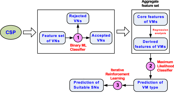
Figure 2: Multi-stage prediction architecture

For each accepted VN, the type of each member VM is predicted. In particular, for a given $G^{v}(N^{v},E^{v})$, each $V_{j}\in G^{v}(N^{v},E^{v})$, $1\leq V_{j}\leq n$ is classified into three categories defined as ”CPU intensive”, ”GPU intensive”, and ”memory intensive” based on the VM configuration and its resource analysis. From the historical VM dataset comprised of features described in IV-A1, a multi-class (three) classifier is trained to estimate the VM type. It is to note that VM requests often arrive with partial information such as CPU and Memory demand represented as $D_{j}^{x}$, where $x\in\{CPU,Memory\}$, VM class $\alpha_{j}$, VM priority $\beta_{j}$. The aforementioned parameters are together called the core VM features. However, certain information may not be made available at the time of VN request arrival and need to be estimated such as end time of VM $\chi_{j}$, actual CPU consumption, actual memory consumption together denoted as $rC_{j}^{x}$, where $x\in\{CPU,memory\}$ etc. Such features are referred to as the derived features. The regression analysis is performed to estimate the most appropriate value of derived features based on the available core features. The core features and derived features together constitute the ”aggregate feature set”.

Upon the classification of each $V_{j}\in G^{v}(N^{v},E^{v})$, $1\leq V_{j}\leq n$ into the predefined VM type, an iterative reinforcement learning is applied for the embedding. Using the Substrate network environment, which represents the current state of the cloud data center, iterative reinforcement learning predicts the most appropriate SNs with sufficient resource availability to embed the VMs in a manner that balances the resource utilization across the cloud data center. Usually, a huge number of parameters are required to optimize on a real-time basis to efficiently manage the cloud data center resources. Since the cloud data center resource configuration dynamically changes with each VN request embedding, it becomes challenging to predict the resource availability on real-time basis for the embedding of incoming new VN requests. Among the RL approaches, Q-learning and SARSA (State-Action-Reward-State-Action) are highly relevant to address the VNE problem. The Q-learning being an off-policy method follows the greedy approach and takes the action, i.e., the selection of the suitable SNs to embed the VMs based on the maximum reward that it can achieve in the current state. However, a greedy approach can lead to the local optimum VNE rather than the global optimum one. Hence, an on-policy RL method SARSA is adopted. Throughout the paper, the actions are referred to as the VNE in the context of the RL. In SARSA, the policy is continuously updated based on the actions it takes. Contrary to the Q-learning, SARSA effectively balances between the exploration and exploitation of the given environment to learn the optimum policy decision.

IV-C Features and predictors

The features and predictors are integral parts of any ML-based algorithm. In this paper, we define two types of features called as core and derived features with respect to VNE in a cloud data center. Often it is considered that the features available at the time of training an ML algorithm, the same set of features are assumed available at the time of testing. However, in many practical applications, it is not the case and the value of a few features are not made available until the execution of the process is concluded. In the context of the VNE, the parameters such as end time of VN and VM, actual resource utilization of VN and VM, are few of the parameters that are not available beforehand and therefore supervised ML algorithms are difficult to apply. In order to tackle the aforementioned problem of feature availability, training is performed in two sequential steps. In the first step, the core features are used and an estimated value of the rest of the derived features are predicted for a given VN request. Later, using the combined set of core and derived features also known as the aggregate set of the features, an ML classifier is trained to obtain the results. The definition of core and derived features is described as follow.

• Core feature set: The set of primary features available at the time of VN and VM request.

• Derived feature set: The set of features, which are not available at the time of VN and VM request, but are derived from the set of core features.

The predictors are commonly known as the set of labels that the algorithm predicts for the given test sample. For the VN feature set, the predictor is a binary value representing the notion ”accepted” and ”rejected”. For the aggregate feature set of VM, the predictor is the multi-class label representing the class ”CPU intensive”, ”GPU intensive”, and ”memory intensive”.

V Knowledge-based model designing

In this section, we design knowledge-based models for efficient VNE.

V-A Binary VN classifier

In this section, we design a supervised support vector binary classifier to classify the VN requests into ”accepted” or ”rejected” using the historical VN dataset. The support vector machine (SVM) is a simple yet robust supervised non-probabilistic binary classifier. The objective of SVM is to find a unique maximum margin hyperplane in a multi-dimensional space that maximizees the margin between two classes and efficiently distinguishes VN request into ”accepted” and ”rejected”. Given the labelled training dataset of VN requests, the SVM generates an optimal hyperplane that categorize the new VN request. On the top of the historical VN dataset, the proposed support vector binary classifier is trained and a representative $\zeta-1$ dimensional hyperplane is constructed in such a way that with respect to the support vectors in class ”accepted” and ”rejected”, the maximum-margin hyperplane is derived. Here, $\zeta$ represents the number of features in VN dataset. Let us assume that the $\varpi$ represents the VN dataset comprised of linearly separable labeled training samples. For simplicity, we redefine VN $G^{v}(N^{v},E^{v})$ as $VN_{v}$.The $\varpi$ can be represented as follow, $\varpi=\{(VN_{1},l_{1}),(VN_{2},l_{2}),...,(VN_{k},l_{k})\}$, where $k$ represents the total number of samples in $\varpi$ and $k>0$. It is to note that $VN_{i}\in\varpi$, $i=\{1,2,...,k\}$ represents $i^{th}$ training VN request comprised of $\zeta$ dimensional feature vector $VN_{f}$. The $l_{i}\in\varpi$, $i=\{1,2,...,k\}$ represents the output class label of $i^{th}$ training sample assigned by CSP. Let us say $l_{i}=1$ represents the output class label ”accepted” and $l_{i}=-1$ represents the output class label ”rejected”. The ultimate goal of the proposed binary classifier is to derive an optimum hyperplane that partitions the training data set $\varpi$ into subsets ”accepted” and ”rejected”. The subset ”accepted” can be defined as $\varpi^{+1}=\{VN_{i}\in\varpi|l_{i}=+1\}$, and the subset ”rejected” can be represented as $\varpi^{-1}=\{VN_{i}\in\varpi|l_{i}=-1\}$, where $\varpi^{+1}\cap\varpi^{-1}=null$. The $l_{i}=+1$ and $l_{i}=-1$ represent the class ”accepted” and ”rejected”, respectively.

For simplicity, let us represent $\aleph_{w,c}(\varpi)$ as a linear classifier. The $\aleph_{w,c}(\varpi)$ can be defined as shown in Eq. 10.

$$\aleph_{w,c}(\varpi)=w^{T}\times VN_{f}+c,~{}~{}~{}\forall VN_{i}\in\varpi$$ (10)

Here, $\aleph_{w,c}(\varpi)$ represents a classification hyperplane, $VN_{f}$ represents $\zeta$-dimensional feature-rule vector corresponding to $VN_{i}$, $w$ represents the $\zeta$-dimensional weight vector associated with feature-rule vector $VN_{f}$, and $c$ represents the bias. The $\zeta$-dimensional weight vector $w$ is a learning vector, which is learned by the classifier from the training dataset $\varpi$.

Three hyper-planes are defined for the classification purpose. The optimized classification hyperplane is represented as $\aleph_{w,c}(\varpi)=w^{T}\times VN_{f}+c=0$. The hyperplane for the nearest data point also known as support vector in class ”accepted” ($l_{i}=+1$) can be represented as $\aleph_{w,c}(\varpi)=w^{T}\times VN_{f}+c=+1$, and the hyperplane for the nearest support vector in class ”rejected” ($l_{i}=-1$) can be represented as $\aleph_{w,c}(\varpi)=w^{T}\times VN_{f}+c=-1$. The distance between hyperplane $\aleph_{w,c}(\varpi)=+1$ and $\aleph_{w,c}(\varpi)=-1$ can be defined as $\dfrac{2}{||w||}$ and is maximized under the constraint $l_{i}(w^{T\times}VN_{f}+c)\geq 1$, for each $VN_{i}\in\varpi$.

In many instances, it is likely that the historical training dataset may not be linearly separable. To tackle such situations, the SVM is extended to include the hinge loss function $max(0,1-l_{i}(w^{T}\times VN_{f}+c))$. In this case, the optimization problem can be defined as shown in Eq. 11, where $\lambda$ decides the margin size and at the same time $\lambda$ ensures that the sample $VN_{i}\in\varpi$ lies in the correct class.

$$min\bigg{(}\bigg{[}\dfrac{1}{m}\sum_{i=1}^{m} max(0,1-l_{i}(w^{T}\times VN_{f}+c))\bigg{]}+\lambda||w||^{2}\bigg{)},$$ (11)

$$where~{}m=number~{}of~{}samples$$

Upon the completion of support vector classifier training, the derived hyperplane is employed to classify the unseen VN test set $\varpi_{Te}$. The VN request $VN_{i}\in\varpi_{Te}$ that classifies into class ”accepted” (+1) is considered as eligible.

V-B Radial Basis Regressors (RBR)

The ”accepted” VNs are further analyzed to build the aggregate feature set of VMs comprised of core features and derived features. Let $\mathbb{D}$ be the historical VM dataset of $N$ data points represented as $(x_{n}$,$y_{n1}$,$y_{n2}$,…$y_{nk})$, $n=\{1,2,..,N\}$. Each data point $(x_{n},y_{n1},y_{n2},...y_{nk})\in\mathbb{D}$ represents a unique historical sample of training dataset. Here, $x_{n}$ represents the core feature set of $n^{th}$ sample, and $y_{n1},y_{n2},...y_{nk}$ represents the observed output value of $k$ derived features in $n^{th}$ training sample. For the estimation of $y_{n1},y_{n2},...y_{nk}$, the regression approach is adopted. Instead of estimating all of the $k$ derived features in a single regression model, $k$ individual regression models are designed to estimate each individual derived feature. Considering the non-linearity nature of the training dataset $\mathbb{D}$, instead of employing linear regression, radial basis function is applied.

The radial basis regressors (RBR) model can be described as follow. Let $\Theta(x)$ be the RBR model trained on the dataset $\mathbb{D}$ and defined as follow.

$$\Theta(x)=\sum_{n=1}^{N}w_{n}\times exp\big{(}-\gamma\lVert x-x_{n}\rVert^{2}\big{)}$$ (12)

Here, $\Theta(x)$ is considered influenced by each training data sample $(x_{n},y_{n1},y_{n2},...y_{nk})$, $n=\{1,2,..\}$ based on the euclidean distance formally defined as $\lVert x-x_{n}\rVert$. In order to smoothen out the distance parameter $\lVert x-x_{n}\rVert$, the $\Theta(x)$ model is embedded with the Gaussian basis function $exp\big{(}-\gamma\lVert x-x_{n}\rVert^{2}\big{)}$. The $\gamma$ is an influential factor. The RBR problem can be transformed into a learning problem to estimate the value of $w_{n}$, $\forall n=\{1,2,...,N\}$ in such a way that for each test sample $(x_{m},y_{mi})$, the $\Theta(x)=y_{mi}$. The learning problem can be formally defined as follow.

The learning problem is reduced to find the $w_{1},w_{2},...,w_{N}$ for Eq. 12 based on the $\mathbb{D}$ in such a way that the Error is minimized (i.e., $\mathbb{E}=0$). In other words, the objective of the learning problem is to obtain $\Theta(x_{n})=y_{mi}$, $\forall n=\{1,2,...,N\}$ as defined in Eq. 13.

$$\sum_{m=1}^{N}w_{m}\times exp\big{(}-\gamma\lVert x_{n}-x_{m}\rVert^{2}\big{)}=y_{mi}$$ (13)

The Eq. 13 can be expanded as shown in Eq. 14.

$$\underbrace{\begin{bmatrix}exp\big{(}-\gamma\lVert x_{1}-x_{1}\rVert^{2}\big{)}&&...&&exp\big{(}-\gamma\lVert x_{1}-x_{N}\rVert^{2}\big{)}\\ exp\big{(}-\gamma\lVert x_{2}-x_{1}\rVert^{2}\big{)}&&...&&exp\big{(}-\gamma\lVert x_{2}-x_{N}\rVert^{2}\big{)}\\ ...&&&&...\\ exp\big{(}-\gamma\lVert x_{N}-x_{1}\rVert^{2}\big{)}&&...&&exp\big{(}-\gamma\lVert x_{N}-x_{N}\rVert^{2}\big{)}\end{bmatrix}}_{\mathbf{\Phi}}\underbrace{\begin{bmatrix}w_{1}\\ w_{2}\\ ...\\ w_{N}\end{bmatrix}}_{\mathbf{w}}=\underbrace{\begin{bmatrix}y_{m1}\\ y_{m2}\\ ...\\ y_{mN}\end{bmatrix}}_{\mathbf{y}}$$ (14)

The exact interpolation or solution may exist if $\Phi$ is invertible. In other words, if $\Phi$ is invertible, the $w$ can be determined as $w=\Phi^{-1}\times y$. By solving the Eq. 13, the estimated value of derived features are obtained.

V-C Maximum Likelihood Classifier (MLC)

Upon obtaining the ”aggregate feature set” of incoming VMs, the same are classified into one of the three categories ”CPU intensive”, ”GPU intensive”, and ”Memory-intensive”. Let $\varsigma$ be the aggregate feature set of VM. It is to note that the historical VM training dataset $\vartheta_{tr}$ is comprised of ”aggregate feature set” along with output label describing the category of the VMs. The supervised Maximum Likelihood Classifier (MLC) is designed based on the features. Let $cL_{j}^{i}$ be the class label of $V_{j}\in G^{v}(N^{v},E^{v})$. Here, $cL_{j}^{i=1}$, $cL_{j}^{i=2}$, and $cL_{j}^{i=3}$ represents the $V_{j}$ of type ”CPU intensive”, ”GPU intensive”, and ”Memory-intensive”, respectively. The historical VM dataset is considered as a training dataset to learn the feature value for each VM category.

For each incoming $V_{j}\in G^{v}(N^{v},E^{v})$, the corresponding aggregate features $\varsigma$ are obtained using RBR model described in Section V-B. Using $\varsigma$, the likelihood probability of class $cL_{j}^{i=1}$, $cL_{j}^{i=2}$, and $cL_{j}^{i=3}$ is calculated using conditional probability. The conditional probability of $cL_{j}^{i=1}$, $cL_{j}^{i=2}$, and $cL_{j}^{i=3}$ can be represented as $p(cL_{j}^{i=1}|\varsigma)$, $p(cL_{j}^{i=1}|\varsigma)$, and $p(cL_{j}^{i=1}|\varsigma)$. For a given aggregate features $\varsigma$ of an incoming VM $V_{j}\in G^{v}(N^{v},E^{v})$, the conditional probability of class $cL_{j}^{i=1}$, $cL_{j}^{i=2}$, and $cL_{j}^{i=3}$ can be calculated as shown in Eq. 15.

$$p(cL_{j}^{i}|\varsigma)=p(cL_{j}^{i}|\varsigma^{1},\varsigma^{2},...,\varsigma^{p}),~{}i\in\{1,2,3\}$$ (15)

Here, $p$ represents the number of features. The feature-rules $\varsigma^{1}$, $\varsigma^{2}$,…,$\varsigma^{p}$ are assumed conditionally independent to each other. In the presence of conditional independence, Eq. 15 can be rewritten as shown in Eq. 16.

$$p(cL_{j}^{i}|\varsigma^{1},\varsigma^{2},...,\varsigma^{p})\propto p(cL_{j}^{i},\varsigma^{1},\varsigma^{2},...,\varsigma^{p})$$ (16)

Further, Eq. 16 can be expanded as shown in Eq. 17.

$$p(cL_{j}^{i}|\varsigma^{1},\varsigma^{2},...,\varsigma^{p})\propto p(cL_{j}^{i})\times p(\varsigma^{1}|cL_{j}^{i})\times p(\varsigma^{2}|cL_{j}^{i})\times...\times p(\varsigma^{p}|cL_{j}^{i})$$ (17)

Here, $p(\varsigma^{k}|cL_{j}^{i})$, $k=\{1,2,...,p\}$ represents the probability of obtaining feature $\varsigma^{k}$ for a given class $cL_{j}^{i}$. The $p(\varsigma^{k}|cL_{j}^{i})$ can be calculated as shown in Eq. V-C.

$$p(\varsigma^{k}|cL_{j}^{i})=\dfrac{1}{\sqrt{2\pi\sigma_{k}^{2}}}\exp\bigg{(}\dfrac{-(\varsigma^{k}-\mu_{k})^{2}}{2\sigma_{k}^{2}}\bigg{)}$$

The $\mu_{k}$ represents the mean value of feature $\varsigma^{k}$ for class $cL_{j}^{i}$. Similarly, $\sigma_{k}^{2}$ represents the standard variance of feature $\varsigma^{k}$ for class $cL_{j}^{i}$. The mean $\mu_{k}$ and standard variance $\sigma_{k}^{2}$ are the learning parameters and they can be estimated from the training set samples of class $cL_{j}^{i}$.

Once the conditional probability model is designed, a Maximum Likelihood Classifier (MLC) is constructed on the top of the model by incorporating Maximum a Posteriori (MAP) decision rule. The classifier function assigns a class label $\widehat{y}=cL_{j}^{i}$ for $i\in\{1,2,3\}$ as shown in Eq. 19.

$$\widehat{y}=\operatorname*{\arg\!\max}_{i\in\{1,2,3\}}p(cL_{j}^{i})\prod_{k=1}^{\lvert\varsigma\rvert}p(\varsigma^{k}|cL_{j}^{i})\}$$ (19)

It is likely that an incoming VM $V_{j}\in G^{v}(N^{v},E^{v})$ classified into class $cL_{j}^{i=1}$, $cL_{j}^{i=1}$, and $cL_{j}^{i=1}$ with equal probability. $p(cL_{j}^{i=1})$=$p(cL_{j}^{i=2})$=$p(cL_{j}^{i=3})$=$\frac{1}{\#~{}of~{}classes}$=$\frac{1}{3}$=$0.33$.

V-D Iterative reinforcement learning

The Reinforcement Learning (RL) is a powerful tool of artificial intelligence, where the system often called as an agent gradually trains itself to act in a manner that yields the incremental reward by means of interacting with the given environment. The RL differs from the established notion of supervised machine learning, where the system learns under the supervision of labelled samples. The RL agent learns in real-time from the given state of the environment to improve the overall outcome. The RL problem is usually considered as a set of sub-optimal actions that together form a Markov Decision Process (MDP). The RL has to walk a tight rope by balancing a trade-off between the exploitation and exploration of the environment. In order to maintain the system performance, the RL agent explores the environment (Cloud data centers) and learns about the existing utilized resources. Subsequently, RL agent exploits the environment to determine the effective action (VNE) that results into positive rewards. To be specific, the RL agent simultaneously explores the environment and exploits the alternative actions that gradually yields the incremental rewards in subsequent actions. The powerful feature of RL is that the learning process looks to achieve a global optimum solution instead of looking for the immediate sub-optimum solution.

Let us consider that RL agent is at the specific state $s_{t}$ of a cloud environment. The agent takes action $a_{t}$ based on the learning, and in response, the cloud environment provides certain reward $r_{t}$ and changes to the new state $\overline{s}_{t}$. Let us denote the aforementioned process as $<s_{t},a_{t},r_{t},\overline{s}_{t}>$. In the context of the proposed VNE in the cloud environment, the action is defined as the selection of SNs for the given configuration of the incoming VMs and the reward is the quality of the embedding. In VNE, the above described process continues and takes finite number of sequences of states, actions and rewards. The entire MDP process can be described as $\{<s_{0},a_{0},r_{0},\overline{s_{1}}>,...,<s_{t},a_{t},r_{t},\overline{s_{t+1}}>,...,<s_{n},a_{n},r_{n},\overline{s_{n+1}}>\}$.

Here, $<s_{t},a_{t},r_{t},\overline{s_{t+1}}>$ describe the $t^{th}$ instance of the action taken by the RL agent, where $s_{t}$ represents the $t^{th}$ state of the cloud environment, $a_{t}$ represents the $t^{th}$ action taken by the RL agent, $r_{t}$ represents the $t^{th}$ reward provided by the environment, and $s_{t+1}$ represents the next $(t+1)^{th}$ state of the environment. The State-action-reward-state-action (SARSA) algorithm is applied to learn the aforementioned Markov decision process. The goal is to update the policy, which is referred to as the optimum state-action value function $Q(s_{t},a_{t})$ based on the action taken by the SARSA agent in a cloud environment as shown in Eq. 20.

$$Q(s_{t},a_{t})\leftarrow Q(s_{t},a_{t})+\alpha\left[r_{t}+\gamma Q(s_{t+1},a_{t+1})-Q(s_{t},a_{t})\right]$$ (20)

Here, $Q(s_{t},a_{t})$ represents the value function for the state $s_{t}$ and action $a_{t}$. The $\alpha\in[0,1]$ represents the learning rate and $\gamma\in[0,1]$ represents the discount factor. Eq. 20 represents the possible reward received in the subsequent step for taking action $a_{t}$ in state $s_{t}$ along with the discounted future reward received in the state $s_{t+1}$ for action $a_{t+1}$. In order to maximize the objective function defined in Eq. III-D, the SARSA agent learns and takes the actions in a manner that maximizes the rewards from the environment. The reward calculation can be described as follow. Upon the classification of VM type, SARSA agent selects the set of SNs that not only satisfy the resource requirement of the VMs in a given VN request but at the same time schedule them onto the appropriate SN type. For example, the CPU intensive VM must be scheduled onto the CPU rich SN along with satisfying the other resource requirements. Based on the action referred to as the VNE by the RL agent, a unique value between -1 to +1 is assigned by the cloud environment indicating the reward to the action. The more the positive reward the better the action was taken by the SARSA agent. The reward is calculated as follow. First, the reward is equally distributed between resource requirement satisfaction and type selection. To be specific, to satisfy the VM type, the agent receives a +0.5 reward. Similarly, for satisfying the resource requirement irrespective of the type, the +0.5 reward is awarded. Again, the +0.5 resource reward is equally divided among each resource type such as CPU, memory, and network. If any one of the resource requirements is not satisfied -0.17 reward is awarded. The example of rewards under different conditions is illustrated in Fig. 3.

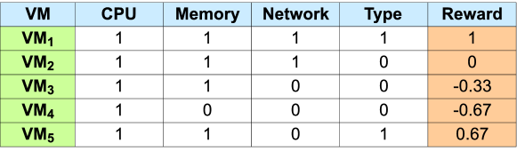
Figure 3: The example calculation of environment reward.

The reward $\mathbb{R}$ of VN $(G^{v}(N^{v},E^{v}))$ can be formally defined as follow.

$$\mathbb{R}(G^{v}(N^{v},E^{v}))=\sum_{V_{j}\in G^{v}(N^{v},E^{v})}\sum_{x\in\{CPU,Memory,Network\}}\mathbb{R}(x)\times\mathbb{H}$$ (21)

Here, $\mathbb{R}$ represents the individual reward received on resource type $x$, and $\mathbb{H}$ represents the decision variable. The $\mathbb{H}$ takes either -1 or +1 value. The $\mathbb{H}$ can be defined formally as follow.

$$\mathbb{H}=\begin{cases}1&A_{i}^{x}=D_{i}^{x}\\ -1&A_{i}^{x}\neq D_{i}^{x}\end{cases}$$

The $\mathbb{R}(x)$ can take value either $0$ or $0.17$.

VI Performance Evaluation and results

In the current section, the performance of the proposed MUVINE scheme is evaluated using the light-weight Java-based discrete event simulator, which is used to generate the substrate network and virtual network requests. Various distribution functions are implemented such as Poisson distribution to simulate the VN request arrival, random distribution to distribute the resources to virtual nodes, virtual links, and substrate network, etc. The performance of the proposed binary VN classifier is compared with the recent admission control algorithm RNN_VNE [30]. The simulation parameters for the SNs, VNs, and VMs are listed in Table II, Table III, and Table IV, respectively.

VI-A Simulation Setup

In this section, the simulation setup for SNs, VNs, and VMs is described in detail. The simulation configuration for the Substrate and Virtual Networks with their resource configuration is taken to suit this small scale simulation environment and for better understanding of the performance evaluation results. However, simulation configuraiton can be extended without any further modification to the simulation environment. Similar simulation configurations were used in our previous works LVRM [7] and DIVYNE [31] in order to rigorously evaluate the VNE embedding schemes. During the simulation, one service provider is considered equipped with 100 SNs connected through links that are generated randomly. For the random links generation, a probability value is set to 0.6, which also acts as the connectivity probability of two SNs. Random distribution is used to allocate the resources to SNs. A randomized function is used to assign the available number of CPUs capacities to each SN ranging from 16 to 32 CPUs. Similarly, the storage and memory capacity are randomly distributed in between 500 GB through 1000 GB, and 20000 MB and 50000 MB, respectively. The available bandwidth between the pairs of SNs is randomly distributed between 1000 Bps and 10000 Bps. The Bps refers to Bytes per second.

In order to generate VN requests, each VN is equipped with VMs in the range of 2 to 10. It is assumed that VN request arrival follows the Poisson distribution with the mean of 5 requests per one hundred time units, and the lifetime of each request follows the exponential distribution with an average lifetime of five hundred time units. It is to note that in a few cases the unexpired lifetime of requests is also considered. The maximum number of virtual links for each request is 45. The number of virtual links is decided by the link probability of 0.6, which also represents the connectivity probability of two VMs. The resource demand for each request is randomly distributed. The number of CPUs demand ranges from 1 through 4. Similarly, the virtual links range from 100 Bps through 500 Bps. The required storage and memory for each VM range from 500 GB to 1000 GB, and 8000 MB to 10000 MB, respectively. The aforementioned simulation setup is repeated several times to ensure sufficient variations in the number of VN requests arrival, types of VN request arrival, amount of resource allocations to VMs etc. A $t-$test is performed on simulation generated dataset to determine the significant difference between random samples. The $P<0.05$ is obtained, which indicates the statistical significance of the simulation dataset.

In the proposed MUVINE scheme, the Scikit-learn [32] open source machine learning library is used to implement the supervised prediction algorithms such as SVM, RBF, and MLC; whereas the implementation of RL is carried out using the TensorFlow software library [33]. In the proposed MUVINE scheme, the SVM, RBF, and MLC are trained on the 66% samples randomly selected from the simulated dataset called as training dataset. On the other hand, the same prediction algorithms are evaluated on remaining 33% of samples also called as testing dataset. The training dataset is comprised of samples that include the features and corresponding real labels. For instance, MUVINE scheme implements the SVM to accept or reject the VN request. Here, each training sample of SVM is comprised of values for VN features described in Section IV-A2 along with a unique label of ”accept” or ”reject”. On the contrary, each test sample is comprised of only values for the VN features and corresponding label is predicted by the SVM. Typically, a loss function is employed to evaluate the performance of supervised algorithms by measuring the distance between the real and predicted label. Contrary to the supervised learning, RL has features without real label of the samples. To be specific, RL does not have dataset, but it works on the given environment. In the current VNE problem, the RL agent works on the cloud environment that includes the VM type, SN type, CPU and memory demand of each VM, available CPU, memory, and bandwidth of each SN etc. The RL explores the states and exploits the all possible actions to predict the most suitable action (i.e., VNE embedding) that results in the improved performance of an evaluation metric also called as reward as defined in Eq. 21. Considering the aforementioned simulation setup, the simulation results are obtained as follows.

TABLE II: The simulation setup for Substrate Nodes (SNs)

Parameters	Value
Total number of SNs = 100
Overall SN resource utilization
Minimum utilization	80%
Maximum utilization	95%
CPU capacity of each SN
Minimum CPU capacity	16
Maximum CPU capacity	32
Memory capacity of each SN (in MB)
Minimum memory capacity	2000
Maximum memory capacity	5000

TABLE III: The simulation setup for Virtual Networks (VNs)

Parameters	Value
Total number of VN requests = 15000
Size of the VN
Minimum number of VMs	2
Maximum number of VMs	10
Other hyper parameters
Start time	0.05 seconds
Mean life time	50 seconds

TABLE IV: The simulation setup for Virtual Machines (VMs)

Parameters	Value
Required memory (in MB) of VM
Minimum required memory	500
Maximum required memory	4096
Required number of CPUs by VM
Minimum number of CPUs	1
Maximum number of CPUs	4
Actual memory usage (in %) by VM
Minimum memory usage	30%
Maximum memory usage	99%
Actual CPU usage (in %) by VM
Minimum CPU usage	30%
Maximum CPU usage	99%
Scheduling class of VM
Minimum scheduling class	1
Maximum scheduling class	3
Priority class of VM
Minimum priority class	1
Maximum priority class	3

VI-B Simulation Results

The simulation of MUVINE scheme is carried out in three stages. Each prediction stage is simulated independently and the simulation results are reported. The simulation results followed by the discussions for each prediction stage are reported as follow.

VI-B1 VN selection accuracy

Upon VN request arrival, the user-defined and CSP-defined parameters are analyzed using the proposed binary SVM classifier denoted as MUVINE_SVM to predict the acceptability of a VN request. For the detailed evaluation, the predictability of MUVINE_SVM is analyzed multi-faceted across the time-domain and across the VN request arrival etc. The prediction outcome of MUVINE_SVM is then compared with the recent Recurrent Neural Network (RNN) based cloud admission control algorithm denoted as RNN_VNE [30].

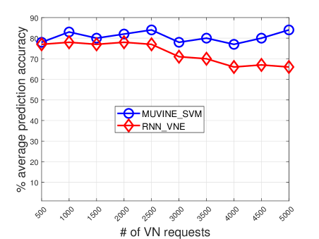
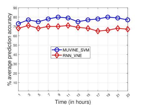
Figure 4: The comparison of average prediction accuracy (in percentage) with respect to (a). number of VN requests, and (b). time (in hours).

Fig. 4a shows the average prediction accuracy (in percentage) of MUVINE_SVM for different number of VN requests. The 5000 test samples are evaluated at the interval of 500 VN requests and corresponding observed prediction accuracy is reported. As shown in Fig. 4a, the average prediction accuracy (in percentage) of the proposed MUVINE_SVM is consistent and as high as 84%. Contrary to the RNN_VNE, the MUVINE_SVM achieves average prediction accuracy improvement of 8%.

Fig. 4b shows the effectiveness of the MUVINE_SVM with respect to the time. The performance of MUVINE_SVM is evaluated for the 24 hours duration and later compared with the RNN_VNE [30]. As shown in Fig. 4b, MUVINE_SVM consistently outputs improved prediction accuracy irrespective of the VN requests’ arrival time. The MUVINE_SVM is robust against the highly fluctuating nature of VN workload arrival. Similar to our previous observation, the proposed MUVINE_SVM shows at least 8.8% higher average prediction accuracy to that of RNN_VNE [30] in the time domain.

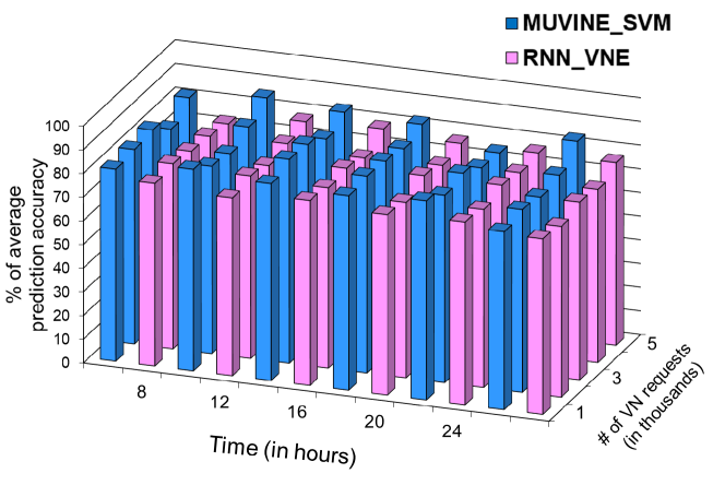
Figure 5: The prediction accuracy of VN requests

For the detailed and extensive performance evaluation, the MUVINE_SVM is simultaneously evaluated against VN request arrival time and number of VN requests together. Fig. 5 shows the outcome of the MUVINE_SVM and RNN_SVM. As shown in Fig. 5, the performance of MUVINE_SVM is consistent and it achieves higher prediction accuracy irrespective of the number of VN requests and their arrival time. The MUVINE_SVM outperforms RNN_VNE [30] with as much as 6.8% higher prediction accuracy across the VN request arrival time and number of VN requests. The possible explanations of SVM outperforming over RNN_VNE are as follow. The MUVINE_SVM is implemented on the top of the carefully selected performance centric VN features discussed in IV-A2, which has empowered the MUVINE_SVM to better distinguish the acceptability of an incoming VN request as compared to the RNN_VNE [30]. Contrary to RNN_VNE, the MUVINE_SVM scales relatively well to the high dimensional data with numerous features, which makes it more suitable to deal with numerous VN requests of cloud environment. When the underlying training and test data can be separated with the hyperplane, the SVM provides a robust outcome with relatively less training and testing time. Considering the VN admission decision as the first stage of the proposed Multi-stage MUVINE scheme, the possible delay leads to the overall delay in VNE. Therefore, the VN predictor is designed with the simpler yet robust alternative to RNN.

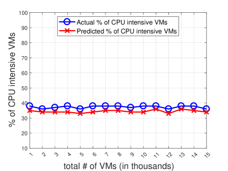
(a) CPU intensive VM class prediction

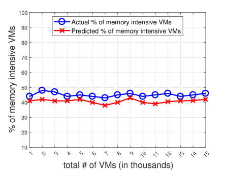
(b) Memory intensive VM class prediction

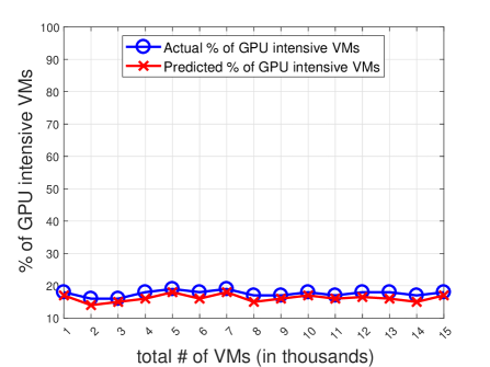
(c) GPU intensive VM class prediction

Figure 6: The performance of Maximum Likelihood Classifier (MLC) for (a). CPU intensive VM class prediction, (b). Memory intensive VM class prediction, (c). GPU intensive VM class prediction.

VI-B2 VM classification accuracy

Upon acceptance of the new VN request, the proposed MUVINE scheme predicts the ”end time” and ”resource utilization” of the corresponding VMs. The ”end time” and ”resource utilization” are the derived features as discussed in Section IV-C. The core and derived features are further used in order to classify the VMs into 3 different categories. The performance of the second stage VM class prediction is presented in Fig. 6. Fig. 6a shows the accuracy of the prediction of CPU intensive VM class by comparing the prediction result with that of the actual VM class. The information of actual VM class is obtained from the CSP post-execution of VN request. The x-axis in Fig. 6a represents the total number of VMs ranging from $1000$ to $15000$; whereas the y-axis represents the percentage of the CPU intensive VMs. The analysis of the simulation dataset reveals that nearly $30\%$ to $40\%$ VMs are the CPU intensive VMs and the rest are either memory intensive or GPU intensive. The simulation result of Fig. 6a shows that the prediction result is quite close to the actual one. From $1000$ VMs, it is predicted that approximately $35\%$ i.e. $350$ VMs belong to CPU intensive class with an error of approximately $7\%$. However, the prediction result marginally improves with the increase in the number of VMs from $1000$ to $15000$. The prediction result shows that approximately $34\%$ VMs are classified as CPU intensive with an error of around $2\%$, which shows the improved classification accuracy.

On the line of the prediction result of CPU intensive VMs, Fig. 6b shows the performance for the memory-intensive VMs. The ground truth from the simulation result reveals that the actual number of memory-intensive VMs ranges between $40\%$ to $48\%$, which is slighly higher than that of the CPU intensive VMs in the simulation data. However, the prediction error ranges between $7\%$ and $3\%$. Out of $1000$ VMs, nearly $41.5\%$ of the VMs are predicted memory intensive in contrast to $44\%$ actual memory-intensive VMs. Similarly, in the case of $15000$ VMs, $42\%$ of the VMs are predicted memory intensive VMs; whereas the number of actual memory-intensive VMs is $45.5\%$. Similar prediction result is observed in the prediction of GPU intensive VMs as in Fig. 6c. The ground truth from the simulation result reveals that the percentage of the actual GPU intensive VMs ranges between $15\%$ and $19\%$. However, predicted percentage of the GPU intensive VMs ranges between $13.5\%$ and $18\%$ with a maximum error $6\%$ and minimum error $1.5\%$.

The noticeable performance of the proposed multi-class Maximum Likelihood Classifier (MLC) can be explained as follows. The proposed MLC is trained on the aggregate features instead of the core one. The inclusion of the derived features makes the underlying aggregate feature set more robust, which empowers the MLC to look for the complex relationship among the VM types and their corresponding feature values. It is to be noted that the proposed MLC independently calculates the likelihood of features for a given VM type. The MLC performs well due to its inherent assumption of conditional independence among the features, which is highly relevant in the cloud environment. For instance, CPU, memory, and GPU intensive VMs have resource requirement that are very specific to the CPU, memory, and GPU, respectively. Therefore, the concerned features dominate more and have least direct relation with other features. The MLC takes the advantage of this cloud property and efficiently predicts the VM classes. The simple to implement yet robust MLC is chosen, considering the requirement of the real-time classification of VMs in the cloud.

VI-B3 VNE evaluation

Upon classifying the VMs, the proposed MUVINE_RL selects the suitable SNs for the embedding purpose. The resource utilization is one of the foremost parameters to evaluate the performance of VNE. The better the resource utilization, the better the VNE. Here, two types of resources are considered for the evaluation such as CPU and Memory. The performance evaluation of MUVINE_RL is carried out with respect to the time domain and number of VMs requests arrival. The performance of the MUVINE_RL is compared with the two traditional state-of-the-art techniques such as Game_Alloc [8] and LVRM [7], and three AI-based techniques such as Auto_RP [6], RL_VNE [34], and RNN_VNE [30].

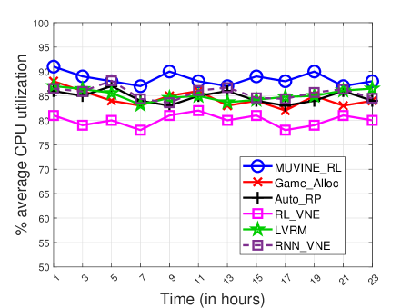
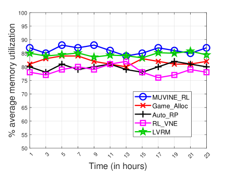
Figure 7: The comparison of average resource utilization (in percentage) with respect to time domain for (a). CPU, (b). Memory.

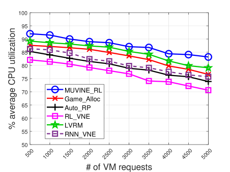
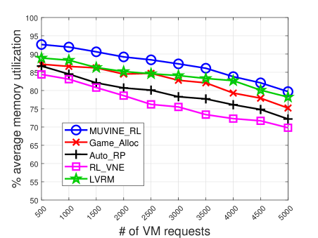
Figure 8: The comparison of average resource utilization (in percentage) with respect to requests for (a). CPU, (b). Memory.

Fig. 7a and Fig. 7b shows the percentage average CPU and memory utilization (in percentage) with respect to the time domain, respectively. With each passing hour, the performance of each VNE scheme is monitored and the CPU and memory utilization are recorded. From Fig. 7a and Fig. 7b, it is clear that all VNE schemes are consistent and they maintain the amount of average CPU and memory utilization in the time domain. However, the average CPU and memory utilization of the Game_Alloc [8], LVRM [7], Auto_RP [6], RL_VNE [34], and RNN_VNE [30] is less as compared to that of MUVINE_RL. The percentage of average utilization of Game_Alloc [8], LVRM [7], Auto_RP [6], RL_VNE [34], RNN_VNE [30], and MUVINE_RL is 83.3%, 85.0%, 79.7%, 76.8%, 85.3%, and 87.6%, respectively. Besides, the MUVINE_RL achieves improved consistency with standard deviation in CPU utilization as low as 2.93 compared to that of 3.7, 3.5, 3.56, 3.8, and 3.1 of Game_Alloc [8], LVRM [7], Auto_RP [6], and RL_VNE [34], RNN_VNE [30], respectively.

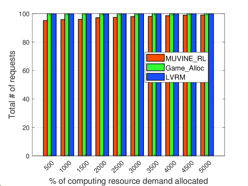
Figure 9: Percentage of computing resource demand allocated

In addition to the time domain evaluation, the VNE should be robust enough to sustain the performance under the varying workload. For that purpose, the existing and proposed schemes are evaluated under the different number of VM requests arrival to know the percentage average CPU and memory utilization. Fig. 8a and Fig. 8b shows the performance comparison of Game_Alloc [8], LVRM [7], Auto_RP [6], RL_VNE [34], and the MUVINE_RL with average CPU and memory utilization, respectively. The RNN_VNE [30] scheme is evaluated for only CPU utilization as it does not focus on the memory aspect. It is to note that contrary to the performance under the time domain, with the increase in the number of VM requests arrival, the percentage average resource utilization decreases gradually for each scheme. With compared to the state-of-the-art existing techniques, the MUVINE_RL improves mean resource utilization by 4.91%.

The improved performance of MUVINE_RL over other schemes can be explained as follows. The primary advantage of MUVINE_RL is its multi-stage prediction model. The improved learning-based admission control of VN requests in the first stage reduces the resource management burden of the CSP and enables the CSP to preserve the resources for the eligible VN requests only. Besides, the maximum likelihood classifier-based VM type prediction in the second stage helps MUVINE_RL to choose the most suitable SNs and subsequently improves the cloud resource utilization. In the absence of VM classification, the MUVINE_RL may end up allocating improper substrate resources to VMs, which may further under-utilize or over-utilize the available substrate resources resulting in the inadequate resource utilization. For example, embedding of CPU intensive VMs onto memory intensive SNs and vice versa greatly influences the cloud resource functioning with reduced overall resource utilization. Although, Auto_RP [6], RL_VNE [34], and RNN_VNE [30] are AI-based schemes, they mainly suffer due to the inclusion of not so important features followed by inadequate information of VM type. This leads to the scenario that the traditional schemes such as Game_Alloc [8], LVRM [7] shows the marginal improvement in the performance over the AI-based schemes. The MUVINE_RL is supported in a three-fold manner from the careful feature selections followed by the prediction of derived features and classification of VMs into respective categories. This leads to the improvement in the overall embedding of VMs and marginally improves the performance in terms of average CPU and memory utilization.

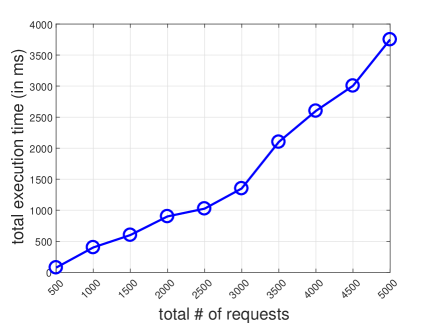
(a) Number of requests vs execution time of proposed scheme.

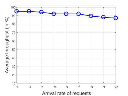
(b) Arrival rate vs throughput of proposed scheme.

Figure 10: Execution time and throughput of proposed scheme.

It is observed that the requests are unable to use cent percent of the total resource allocated to them. In the proposed MUVINE scheme, the amount of resource allocated is greater than or equal to the amount of resource required by the request. As a result, resource utilization is less, which refers to the ratio of resource allocated and the amount of resource being used. The MUVINE_RL investigate this issue and allocate the resource according to resource usage prediction. Fig. 9 shows the comparison result of the MUVINE_RL with two recent traditional VNE schemes. The x-axis and the y-axis in Fig. 9 represent the number of requests and the percentage of computing resource demand allocated, respectively. Here requests refer to the virtual network and computing resource refers to the CPU resource and memory resource. Both the traditional VNE schemes allocate exactly the same amount of the resource requested by the VNs. However, the MUVINE_RL allocates less amount of resources than the demand. For $500$ requests a total of $95.3\%$ of the total resource demand is allocated to the requests. However, as the number of requests increases to $5000$ a total of $98.8\%$ of the requested resource are allocated to the VNs.

The performance of the MUVINE_RL is evaluated in terms of the total execution time and the throughput, as shown in Fig. 10(a) and 10(b), respectively. The total execution time, which is measured in milliseconds (ms), is observed when the total number of requests increases from $500$ to $5000$. It is observed that the MUVINE_RL takes total execution time of approximately $75ms$ to process $500$ requests. However, the execution time increases very rapidly to approximately $400ms$ when the number of requests is doubled. This rapid increase is due to the randomness of the number of VMs in each request. From the investigation, it is found that the average number of VMs in the first $500$ requests is $3.7$, whereas the average number of VMs in the next $500$ requests only is $7.67$. The total execution time to process $5000$ requests is observed to be $3750ms$, as shown in Fig. 10(a). Similarly, to evaluate the performance of the MUVINE_RL, the throughput is also observed as shown in Fig. 10(b). The throughput is observed in percentage (in y-axis) with the varied arrival rate of the requests (in x-axis). Throughput refers to the percentage of the total requests that are processed in a single time unit. Arrival rate indicated the number of requests arrived per unit time. The throughput decreases when the arrival increases. The throughput of the MUVINE_RL is $96\%$ when the arrival rate is $2$ requests per unit time. However, the throughput decreases to approximately $88\%$ when the arrival rate increases to $10$ requests per unit time, as shown in Fig. 10(b).

VII Conclusions

In this paper, we deal with the real-time virtual network embedding problem. Accordingly, Reinforcement Learning based prediction models are designed for the Multi-stage Virtual Network Embedding (MUVINE) in cloud data centers. Using the historical supervised data, the acceptability of real-time incoming VNs is ascertained using binary supervised classifier followed by identification of the type of each individual VM. The information of VM type is used by designing a SARSA reinforcement learning agent that improves the cloud resource utilization by embedding the VMs onto the suitable SNs. The binary VN classifier acts as an admission control and it significantly improves the cloud performance by rejecting infeasible requests and forwards only those with higher probability to be accepted. The Radial Basis Regressor (RBR) model is designed to predict the derived features. The entire MUVINE scheme is designed in such a way that each prediction stage contributes towards identifying the appropriate substrate resources for the given virtual resource demand. Each stage of the prediction model is extensively simulated and is evaluated to compare the results with similar state-of-the-art traditional and AI-based approaches. The simulation results clearly demonstrate the superiority of our proposed prediction model over others with consistent outcome across the time domain and number of virtual requests. However, for further verification and improvement, we strive to implement the proposed model in the real cloud environment, which will be part of our future work.

References

- [1] Dong Zhang, Shuhui Li, Min Sun, and Zheng O’Neill. An optimal and learning-based demand response and home energy management system. IEEE Transactions on Smart Grid, 7(4):1790–1801, 2016.
- [2] Shai Shalev-Shwartz, Shaked Shammah, and Amnon Shashua. Safe, multi-agent, reinforcement learning for autonomous driving. arXiv preprint arXiv:1610.03295, 2016.
- [3] Hiren Kumar Thakkar and Prasan Kumar Sahoo. Towards automatic and fast annotation of seismocardiogram signals using machine learning. IEEE Sensors Journal, 2019.
- [4] Rashid Mijumbi, Juan-Luis Gorricho, Joan Serrat, Meng Shen, Ke Xu, and Kun Yang. A neuro-fuzzy approach to self-management of virtual network resources. Expert systems with applications, 42(3):1376–1390, 2015.
- [5] A. Alsarhan, A. Itradat, A. Y. Al-Dubai, A. Y. Zomaya, and G. Min. Adaptive resource allocation and provisioning in multi-service cloud environments. IEEE Transactions on Parallel and Distributed Systems, 29(1):31–42, Jan 2018.
- [6] Mostafa Ghobaei-Arani, Sam Jabbehdari, and Mohammad Ali Pourmina. An autonomic resource provisioning approach for service-based cloud applications: A hybrid approach. Future Generation Computer Systems, 78:191 – 210, 2018.
- [7] P. K. Sahoo, C. K. Dehury, and B. Veeravalli. Lvrm: On the design of efficient link based virtual resource management algorithm for cloud platforms. IEEE Transactions on Parallel and Distributed Systems, 29(4):887–900, April 2018.
- [8] W. Wei, X. Fan, H. Song, X. Fan, and J. Yang. Imperfect information dynamic stackelberg game based resource allocation using hidden markov for cloud computing. IEEE Transactions on Services Computing, 11(1):78–89, Jan 2018.
- [9] Yongqiang Gao, Haibing Guan, Zhengwei Qi, Yang Hou, and Liang Liu. A multi-objective ant colony system algorithm for virtual machine placement in cloud computing. Journal of Computer and System Sciences, 79(8):1230–1242, 2013.
- [10] An Song, Wei-Neng Chen, Tianlong Gu, Huaxiang Zhang, and Jun Zhang. A constructive particle swarm optimizer for virtual network embedding. IEEE Transactions on Network Science and Engineering, 2019.
- [11] Mansaf Alam, Kashish Ara Shakil, and Shuchi Sethi. Analysis and clustering of workload in google cluster trace based on resource usage. CoRR, abs/1501.01426, 2015.
- [12] Wenfeng Xia, Peng Zhao, Yonggang Wen, and Haiyong Xie. A survey on data center networking (dcn): Infrastructure and operations. IEEE communications surveys & tutorials, 19(1):640–656, 2017.
- [13] Peiying Zhang, Haipeng Yao, and Yunjie Liu. Virtual network embedding based on the degree and clustering coefficient information. IEEE Access, 4:8572–8580, 2016.
- [14] Chan Kyu Pyoung and Seung Jun Baek. Joint load balancing and energy saving algorithm for virtual network embedding in infrastructure providers. Computer Communications, 121:1–18, 2018.
- [15] Soroush Haeri and Ljiljana Trajkovic. Virtual network embedding via monte carlo tree search. IEEE Transactions on Cybernetics, PP(99):1–12, 2017.
- [16] F. Esposito, I. Matta, and Y. Wang. Vinea: An architecture for virtual network embedding policy programmability. IEEE Transactions on Parallel and Distributed Systems, 27(11):3381–3396, Nov 2016.
- [17] N. Shahriar, S. R. Chowdhury, R. Ahmed, A. Khan, S. Fathi, R. Boutaba, J. Mitra, and L. Liu. Virtual network survivability through joint spare capacity allocation and embedding. IEEE Journal on Selected Areas in Communications, pages 1–1, 2018.
- [18] Jiangtao Zhang, Hejiao Huang, and Xuan Wang. Resource provision algorithms in cloud computing: A survey. Journal of Network and Computer Applications, 64:23–42, 2016.
- [19] Atakan Aral and Tolga Ovatman. Network-aware embedding of virtual machine clusters onto federated cloud infrastructure. Journal of Systems and Software, 120:89 – 104, 2016.
- [20] Long Gong, Huihui Jiang, Yixiang Wang, and Zuqing Zhu. Novel location-constrained virtual network embedding LC-VNE algorithms towards integrated node and link mapping. IEEE/ACM Transactions on Networking, 24(6):3648–3661, dec 2016.
- [21] Lei Yin, Zheng Chen, Ling Qiu, and Yonggang Wen. Interference based virtual network embedding. In 2016 IEEE International Conference on Communications (ICC). IEEE, may 2016.
- [22] An Song, Wei-Neng Chen, Yue-Jiao Gong, Xiaonan Luo, and Jun Zhang. A divide-and-conquer evolutionary algorithm for large-scale virtual network embedding. IEEE Transactions on Evolutionary Computation, 2019.
- [23] An Song, Wei-Neng Chen, Tianlong Gu, Huaqiang Yuan, Sam Kwong, and Jun Zhang. Distributed virtual network embedding system with historical archives and set-based particle swarm optimization. IEEE Transactions on Systems, Man, and Cybernetics: Systems, 2019.
- [24] Haipeng Yao, Xu Chen, Maozhen Li, Peiying Zhang, and Luyao Wang. A novel reinforcement learning algorithm for virtual network embedding. Neurocomputing, 284:1 – 9, 2018.
- [25] Yu Zhang, Jianguo Yao, and Haibing Guan. Intelligent cloud resource management with deep reinforcement learning. IEEE Cloud Computing, 4(6):60–69, 2018.
- [26] Cong Wang, Fanghui Zheng, Sancheng Peng, Zejie Tian, Yujia Guo, and Ying Yuan. A coordinated two-stages virtual network embedding algorithm based on reinforcement learning. In 2019 Seventh International Conference on Advanced Cloud and Big Data (CBD), pages 43–48. IEEE, 2019.
- [27] Haipeng Yao, Bo Zhang, Peiying Zhang, Sheng Wu, Chunxiao Jiang, and Song Guo. Rdam: A reinforcement learning based dynamic attribute matrix representation for virtual network embedding. IEEE Transactions on Emerging Topics in Computing, 2018.
- [28] Q. Zhang, L. T. Yang, Z. Yan, Z. Chen, and P. Li. An efficient deep learning model to predict cloud workload for industry informatics. IEEE Transactions on Industrial Informatics, 14(7):3170–3178, July 2018.
- [29] Santwana Sagnika, Saurabh Bilgaiyan, and Bhabani Shankar Prasad Mishra. Workflow scheduling in cloud computing environment using bat algorithm. In Proceedings of First International Conference on Smart System, Innovations and Computing, pages 149–163. Springer, 2018.
- [30] Andreas Blenk, Patrick Kalmbach, Patrick Van Der Smagt, and Wolfgang Kellerer. Boost online virtual network embedding: Using neural networks for admission control. In Network and Service Management (CNSM), 2016 12th International Conference on, pages 10–18. IEEE, 2016.
- [31] Chinmaya Kumar Dehury and Prasan Kumar Sahoo. Dyvine: Fitness-based dynamic virtual network embedding in cloud computing. IEEE Journal on Selected Areas in Communications, 37(5):1029–1045, 2019.
- [32] F. Pedregosa, G. Varoquaux, A. Gramfort, V. Michel, B. Thirion, O. Grisel, M. Blondel, P. Prettenhofer, R. Weiss, V. Dubourg, J. Vanderplas, A. Passos, D. Cournapeau, M. Brucher, M. Perrot, and E. Duchesnay. Scikit-learn: Machine learning in Python. Journal of Machine Learning Research, 12:2825–2830, 2011.
- [33] M Abadi, A Agarwal, P Barham, E Brevdo, Z Chen, C Citro, GS Corrado, A Davis, J Dean, M Devin, et al. Tensorflow: large-scale machine learning on heterogeneous distributed systems. arxiv preprint (2016). arXiv preprint arXiv:1603.04467.
- [34] Haipeng Yao, Xu Chen, Maozhen Li, Peiying Zhang, and Luyao Wang. A novel reinforcement learning algorithm for virtual network embedding. Neurocomputing, 284:1–9, 2018.