A Locally Stable Edit Distance for Merge Trees

Abstract

In this paper we define a novel edit distance for merge trees and compare it with other metrics appearing in the literature. Then we consider the metric space obtained and study the properties of such space obtaining completeness and compactness results, the existence of Frechét Means and local parametrizations by means of euclidean spaces. Whilst doing so, we explore the geodesic structure of the space of merge trees, stratifying trees by means of their dimension and decomposing geodesics along different strata. All these results contribute to understanding how the different strata interact, which is pivotal for the development of more refined tools and techniques for merge trees.

Keywords: Topological Data Analysis, Merge Trees, Frechét Means, Geodesics, Tree Edit Distance

1 Introduction

Topological Data Analysis (TDA) is a particular set of techniques within the field of geometric data analysis which aim at including topological information into data analysis pipelines.

Topological information is usually understood in terms of generators of homology groups (Hatcher, 2000) with coefficients in some field. With persistent homology these generators are extracted along a filtration of topological spaces to capture the shape of the initial datum, typically a function or a point cloud, at “different resolutions” (Edelsbrunner and Harer, 2008). To proceed with the analysis, this ordered family of vector spaces is then represented with a topological summary. There are many different kinds of topological summaries such as persistence diagrams (Edelsbrunner et al., 2002), persistence images (Adams et al., 2017), persistence silhouettes (Chazal et al., 2015), and persistence landscapes (Bubenik, 2015). Each of these summaries live in a space with different properties and purposes: for instance persistence diagrams are highly interpretable and live in a metric space, persistence landscapes are embedded in a linear space of functions, but the embedding is not closed under linear combinations, persistence images are instead obtained as vectors in $\mathbb{R}^{n}$, making them suitable for many Machine Learning techniques.

Along with the aforementioned summaries, there are also tree-shaped objects called merge trees. Merge trees arise naturally within the framework of TDA when dealing with zero dimensional homology groups, as they capture the merging structure of path connected components along a filtration of topological spaces. Originally, such objects stem out of Morse Theory (Milnor, 2016) as a topological summary related to Reeb graphs (Shinagawa et al., 1991; Biasotti et al., 2008) and are frequently used for data visualization purposes (wu and Zhang, 2013; Bock et al., 2017). Analogously, other different but related kinds of trees like hierarchical clustering dendrograms (Murtagh and Contreras, 2017) or phylogenetic trees (Felsenstein and Felenstein, 2004) have also been used extensively in statistics and biology to infer information about a fixed set of labels. When considered as unlabelled objects, however, both clustering dendrograms and phylogenetic trees can be obtained as particular instances of merge trees.

The uprising of TDA has propelled works aiming at using merge trees and Reeb graphs as topological summaries in data analysis contexts and thus developing metrics and frameworks to analyze populations of such objects (Beketayev et al., 2014; Morozov et al., 2013; Gasparovic et al., 2019; Touli, 2020; Sridharamurthy et al., 2020; Wetzels et al., 2022; Di Fabio and Landi, 2016; Bauer et al., 2020).

Returning to the typical TDA pipeline, once a topological representation suitable for the analysis is chosen the tools that can be employed are a direct consequence of the properties of the space the summaries live in, as for any other data analysis situation. For instance, many statistical techniques rely on the linear structure of Euclidean spaces: typical examples are linear regression and principal components analysis (PCA). However, there are many examples of analyses carried out on data not lying (at least naively) in $\mathbb{R}^{n}$ or other vector spaces. Quotient spaces of functions up to reparametrization, point clouds up to isometries, probability distributions, matrices up to some kind of base change etc. all require complex mathematical frameworks to be treated, since even things like moving from one point to another must be carefully defined. For these reasons there has been a lot of effort in generalizing statistical tools for data living outside Euclidean spaces. The most commonly considered generalization is the case of data being sampled from Riemannian manifolds - often Lie Groups - (Pennec, 2006; Pennec et al., 2019; Pennec, 2018; Huckemann and Eltzner, 2018; Huckemann et al., 2010; Jung et al., 2012; Thomas Fletcher, 2013; Patrangenaru and Ellingson, 2015), where the richness of the Riemannian structure is fundamental to develop techniques and results. The situation becomes further challenging when one cannot build a differential or even a topological structure which falls into the realm of well-known and deeply studied geometrical objects like manifolds. In this case ad-hoc, meaningful tools and definitions must be carefully obtained in order to be able to work in such spaces (Mileyko et al., 2011; Leygonie et al., 2021b; Calissano et al., 2020; Miller et al., 2015; Garba et al., 2021).

Related Works

The works that have been dealing with the specific topic of merge trees can be divided into two groups: the first group is more focused on the definition of a suitable metric structure on merge trees and the second is more focused on the properties of merge trees and their relationships with persistence diagrams. The first group, in turns, splits into a) works dealing with the interleaving distance between merge trees and other metrics with very strong - universal - theoretical properties (Beketayev et al., 2014; Morozov et al., 2013; Touli and Wang, 2018; Gasparovic et al., 2019; Touli, 2020; Curry et al., 2022; Cardona et al., 2021), b) metrics which are more focused on the computational efficiency (Sridharamurthy et al., 2020; Wetzels et al., 2022; Pont et al., 2022) at the cost of sacrificing stability properties and trying to mitigate the resulting problems with pre-processing and other computational solutions. The second stream of research, instead, investigates structural properties of merge trees, answering questions like how many merge trees share the same persistence diagram (Kanari et al., 2020; Curry et al., 2021; Beers and Leygonie, 2023), defining function spaces on merge trees (Pegoraro, 2021b) and obtaining other structures which lie in between persistence diagrams and merge trees (Elkin and Kurlin, 2021).

Main Contributions

The aim of this manuscript is to propose a novel metric for merge trees and to investigate some geometric properties of the resulting metric space of merge trees. Such investigation is intended as a first step into the development of statistical tools to analyze sets of such objects, in analogy with what has already been done for persistence diagrams (Mileyko et al., 2011; Turner et al., 2014; Bubenik and Wagner, 2020; Che et al., 2021) and other kinds of trees (Billera et al., 2001; Miller et al., 2015; Garba et al., 2021).

The metric which is proposed is based on a more general edit distance between weighted (in a broad sense) trees which is developed in Pegoraro (2023): such work contains the main theoretic results which allow us to define the new distance and the algorithm which is used to compute it. This edit distance is very different from other edit distances which have been proposed for merge trees for two reasons: 1) it does not measure differences between trees in terms of persistence pairs (as opposed to Sridharamurthy et al. (2020) and Pont et al. (2022)) but in terms of edge length, resulting in a different way in which variability between trees is captured; 2) the edit operations which characterize this distance are more flexible than the usual ones, with some operations being a complete novelty with respect to the existing literature on general edit distances. This on one side causes a higher computational cost, but allows for suitable stability properties, which are investigated and proved in Pegoraro and Secchi (2021).

As already mentioned, the general aim of our geometric investigation is to obtain a better understanding of the local behaviour of the metric space of merge trees, to better grasp the mathematical and statistical possibilities offered by that space. In particular, we focus our geometric analysis on three directions. First we obtain a series of topological results which lead to the definition of $0$-dimensional summaries of empirical distributions of merge trees, via their Frechét means - sometimes called Karcher means - (Karcher, 1977): these objects generalize the widely used euclidean means and can be seen as the most basic statistics employed in data analysis, but that can provide important results even outside the euclidean context (Davis, 2008; Pennec, 2018). Second, we start studying the metric structure of the space of merge trees, with results on the local uniqueness of its geodesic paths. Third we provide some tools to have a local linear approximation of the space of merge trees, via a decomposition of its geodesics along different strata of the space. With such local parametrizations, we are able to propose an approximation scheme for Frechét means.

Outline

This paper is organized as follows. Section 2, Section 3 and Section 4 contain the preliminary definitions needed in the paper, which are collected from previous works in the field. In the latter one, in particular, we review the definition of the edit distance between weighted trees, which we use in Section 5 to define a metric structure for merge trees. In Section 6 we discuss some geometric properties of the metric space obtained, with particular focus on geodesic structure, compact sets, Frechét Means and local parametrizations of the space of trees via some euclidean space. In Section 7 we draw some conclusions.

The appendices contain Section B which features an in depth investigation of some characteristics of the edit distance along with a detailed comparison with other established metrics for merge trees. While Section C contains the proofs of the results in the manuscript.

2 Preliminary Definitions - Merge Trees

This is the first of three preliminary sections to our work. Here, following Patel (2018), Curry et al. (2022) and Pegoraro (2021b) we introduce most of the objects we need for our investigation, reporting definitions which are well established in TDA. The other preliminary sections will focus on recalling metric geometry terminology/results and the edit distance defined in Pegoraro (2021b).

Figure 1 illustrates some of the objects we introduce in this section.

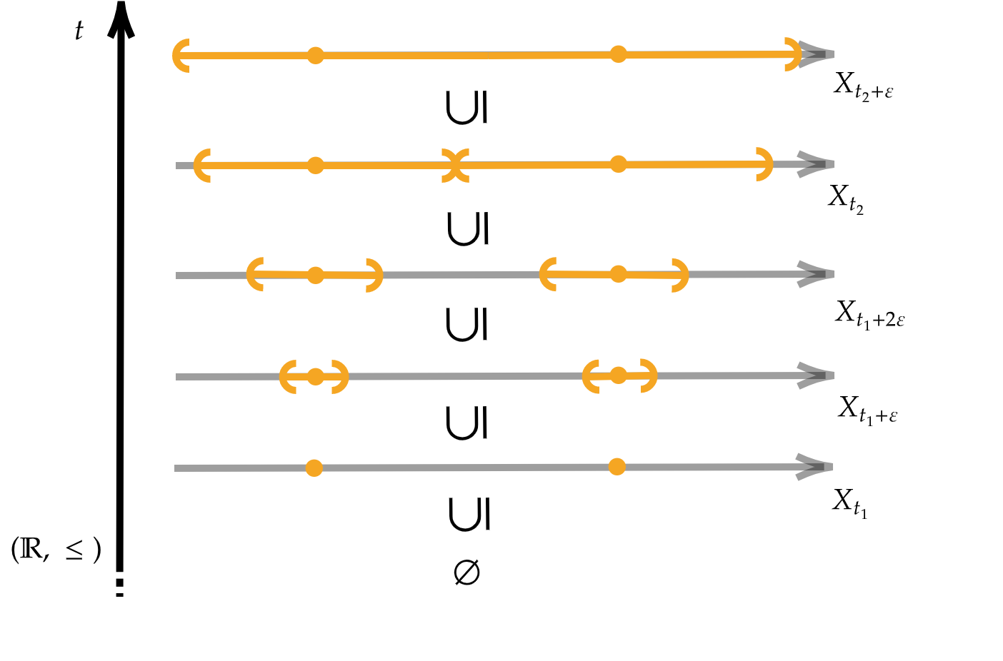
(a) A filtration $X_{\operatorname*{\scalerel*{\cdot}{\bigodot}}}$.

(b) An abstract merge tree $\pi_{0}(X_{\operatorname*{\scalerel*{\cdot}{\bigodot}}})$.

(c) A regular abstract merge tree $\pi_{0}(X_{\operatorname*{\scalerel*{\cdot}{\bigodot}}})$.

(d) The merge tree $\mathcal{M}(\pi_{0}(X_{\operatorname*{\scalerel*{\cdot}{\bigodot}}}))$ with $\pi_{0}(X_{\operatorname*{\scalerel*{\cdot}{\bigodot}}})$ as in Figure 1(c).

Figure 1: On the first line we see an example of a filtration along with its abstract merge tree. in In the bottom line there are a regular abstract merge tree and the associated merge tree. The colors are used throughout the plots to highlight the relationships between the different objects.

Definition 1 (Curry et al. (2022))

A filtration of topological spaces is a (covariant) functor $X_{\operatorname*{\scalerel*{\cdot}{\bigodot}}}:\mathbb{R}\rightarrow\operatorname*{Top}$ from the poset $(\mathbb{R},\leq)$ to $\operatorname*{Top}$, the category of topological spaces with continuous functions, such that: $X_{t}\rightarrow X_{t^{\prime}}$, for $t<t^{\prime}$, are injective maps.

Example

Given a real valued function $f:X\rightarrow\mathbb{R}$ the sublevel set filtration is given by $X_{t}=f^{-1}((-\infty,t])$ and $X_{t<t^{\prime}}=i:f^{-1}((-\infty,t])\hookrightarrow f^{-1}((-\infty,t^{\prime}])$.

Example

Given a finite set $C\subset\mathbb{R}^{n}$ its the Céch filtration is given by $X_{t}=\bigcup_{c\in C}B_{t}(c)$. With $B_{t}(c)=\{x\in\mathbb{R}^{n}\mid\parallel c-x\parallel<t\}$. As before: $X_{t<t^{\prime}}=i:\bigcup_{c\in C}B_{t}(c)\hookrightarrow\bigcup_{c\in C}B_{t^{\prime}}(c)$.

Given a filtration $X_{\operatorname*{\scalerel*{\cdot}{\bigodot}}}$ we can compose it with the functor $\pi_{0}$ sending each topological space into the set of its path connected components. We recall that, according to standard topological notation, $\pi_{0}(X)$ is the set of the path connected components of $X$ and, given a continuous functions $q:X\rightarrow Y$, $\pi_{0}(q):\pi_{0}(X)\rightarrow\pi_{0}(Y)$ is defined as:

$$U\mapsto V\text{ such that }q(U)\subset V.$$

Definition 2 (Carlsson and Mémoli (2013); Curry (2018))

A persistent set is a functor $S:\mathbb{R}\rightarrow\operatorname*{Sets}$. In particular, given a filtration of topological spaces $X_{\operatorname*{\scalerel*{\cdot}{\bigodot}}}$, the persistent set of components of $X_{\operatorname*{\scalerel*{\cdot}{\bigodot}}}$ is $\pi_{0}\circ X_{\operatorname*{\scalerel*{\cdot}{\bigodot}}}$. A one dimensional persistent module is a functor $S:\mathbb{R}\rightarrow\operatorname*{Vec}_{\mathbb{K}}$ with values in the category of vector spaces $\operatorname*{Vec}_{\mathbb{K}}$.

By endowing a persistent set with the discrete topology, every persistence set can be seen as the persistence set of components of a filtration. Thus a general persistent set $S$ can be written as $\pi_{0}(X_{\operatorname*{\scalerel*{\cdot}{\bigodot}}})$ for some filtration $X_{\operatorname*{\scalerel*{\cdot}{\bigodot}}}$.

Based on the notion of constructible persistent sets found in Patel (2018) and Curry et al. (2022) one then builds the following objects.

Definition 3 (Pegoraro (2021b))

An abstract merge tree is a persistent set $S:\mathbb{R}\rightarrow\operatorname*{Sets}$ such that there is a finite collection of real numbers $\{t_{1}<t_{2}<\ldots<t_{n}\}$ which satisfy:

• $S(t)=\emptyset$ for all $t<t_{1}$;

• $S(t)=\{\star\}$ for all $t>t_{n}$;

• if $t,t^{\prime}\in(t_{i},t_{i+1})$, with $t<t^{\prime}$, then $S(t<t^{\prime})$ is bijective.

The values $\{t_{1}<t_{2}<\ldots<t_{n}\}$ are called critical values of the tree and there is always a minimal set of critical values (Pegoraro, 2021b). We always assume to be working with such minimal set.

If $S(t)$ is always a finite set, $S$ is a finite abstract merge tree.

Consider an abstract merge tree $\pi_{0}(X_{\operatorname*{\scalerel*{\cdot}{\bigodot}}})$ and let $t_{1}<t_{2}<\ldots<t_{n}$ be its (minimal set of) critical values and let $i_{t}^{t^{\prime}}:=X_{t\leq t^{\prime}}:X_{t}\rightarrow X_{t^{\prime}}$. Take $\varepsilon>0$ small. We have that at least one between $\pi_{0}(i_{t_{j}-\varepsilon}^{t_{j}})$ and $\pi_{0}(i_{t_{j}}^{t_{j}+\varepsilon})$ is not bijective. So we have the following definition.

Definition 4 (Pegoraro (2021b))

An abstract merge tree $\pi_{0}(X_{\operatorname*{\scalerel*{\cdot}{\bigodot}}})$ is said to be regular if $\pi_{0}(i_{t_{j}}^{t_{j}+\varepsilon})$ is bijective for every critical value $t_{j}$ and for every $\varepsilon>0$ small enough.

Assumption 1

From now on we consider only regular abstract merge trees. In Pegoraro (2021b) it is shown that this choice is non-restrictive.

Now we introduce merge trees with the approach found in Pegoraro (2021b) - from which we take the upcoming definitions. A combinatorial object, called tree structure, is introduced, and we add to it some height values with a function. Similar approaches can be found in most of the scientific literature dealing with such topics (Gasparovic et al., 2019; Sridharamurthy et al., 2020; Wetzels et al., 2022; Pont et al., 2022).

Definition 5

A tree structure $T$ is given by a set of vertices $V_{T}$ and a set of edges $E_{T}\subset V_{T}\times V_{T}$ which form a connected rooted acyclic graph. We indicate the root of the tree with $r_{T}$. We say that $T$ is finite if $V_{T}$ is finite. The order of a vertex $v\in V_{T}$ is the number of edges which have that vertex as one of the extremes, and is called $ord_{T}(v)$. Any vertex with an edge connecting it to the root is its child and the root is its father: this is the first step of a recursion which defines the father and children relationship for all vertices in $V_{T}.$ The vertices with no children are called leaves or taxa and are collected in the set $L_{T}$. The relation $child<father$ generates a partial order on $V_{T}$. The edges in $E_{T}$ are identified in the form of ordered couples $(a,b)$ with $a<b$. A subtree of a vertex $v$, called $sub_{T}(v)$, is the tree structure whose set of vertices is $\{x\in V_{T}|x\leq v\}$.

Given a tree structure $T$, identifying an edge $(v,v^{\prime})$ with its lower vertex $v$, gives a bijection between $V_{T}-\{r_{T}\}$ and $E_{T}$, that is $E_{T}\cong V_{T}-\{r_{T}\}$ as sets. Given this bijection, we often use $E_{T}$ to indicate the vertices $v\in V_{T}-\{r_{T}\}$, to simplify the notation.

The following isomorphism classes are introduced to identify merge trees independently of their vertex set.

Definition 6

Two tree structures $T$ and $T^{\prime}$ are isomorphic if exists a bijection $\eta:V_{T}\rightarrow V_{T^{\prime}}$ that induces a bijection between the edges sets $E_{T}$ and $E_{T^{\prime}}$: $(a,b)\mapsto(\eta(a),\eta(b))$. Such $\eta$ is an isomorphism of tree structures.

Then, we can give the definition of a merge tree.

Definition 7

A merge tree is a finite tree structure $T$ with a monotone increasing height function $h_{T}:V_{T}\rightarrow\mathbb{R}\cup\{+\infty\}$ and such that 1) $ord_{T}(r_{T})=1$ 2) $h_{T}(r_{T})=+\infty$ 3) $h_{T}(v)\in\mathbb{R}$ for every $v<r_{T}$. The set of all merge trees is called $\mathcal{MT}$.

Two merge trees $(T,h_{T})$ and $(T^{\prime},h_{T^{\prime}})$ are isomorphic if $T$ and $T^{\prime}$ are isomorphic as tree structures and the isomorphism $\eta:V_{T}\rightarrow V_{T^{\prime}}$ is such that $h_{T}=h_{T^{\prime}}\circ\eta$. Such $\eta$ is an isomorphism of merge trees. We use the notation $(T,h_{T})\cong(T^{\prime},h_{T^{\prime}})$.

With some slight abuse of notation we set $\max h_{T}=\max_{v\in V_{T}\mid v<r_{T}}h_{T}(v)$ and $\arg\max h_{T}=\max\{v\in V_{T}\mid v<r_{T}\}$. Note that, given $(T,h_{T})$ merge tree, there is only one edge of the form $(v,r_{T})$ and we have $v=\arg\max h_{T}$.

Definition 8

Given a tree structure $T$, we can eliminate an order two vertex, connecting the two adjacent edges which arrive and depart from it. Suppose we have two edges $e=(v_{1},v_{2})$ and $e^{\prime}=(v_{2},v_{3})$, with $v_{1}<v_{2}<v_{3}$. And suppose $v_{2}$ is of order two. Then, we can remove $v_{2}$ and merge $e$ and $e^{\prime}$ into a new edge $e^{\prime\prime}=(v_{1},v_{3})$. This operation is called the ghosting of the vertex. Its inverse transformation is called the splitting of an edge.

Consider a merge tree $(T,h_{T})$ and obtain $T^{\prime}$ by ghosting a vertex of $T$. Then $V_{T^{\prime}}\subset V_{T}$ and thus we can define $h_{T^{\prime}}:=h_{T\mid V_{T^{\prime}}}$.

Now we can state the following definition.

Definition 9

Merge trees are equal up to order $2$ vertices if they become isomorphic after applying a finite number of ghostings or splittings. We write $(T,h_{T})\cong_{2}(T^{\prime},h_{T^{\prime}})$.

We report a result summarizing the relationship between abstract merge trees and merge trees. The main consequence of such result is that merge trees considered up to order $2$ vertices are an appropriate discrete tool to represent the information contained in regular abstract merge trees. Figure 1(b) and Figure 1(d) can help the reader going through the following proposition.

Proposition 1 (Pegoraro (2021b))

The following hold:

1. we can associate a merge tree without order $2$ vertices $\mathcal{M}(\pi_{0}(X_{\operatorname*{\scalerel*{\cdot}{\bigodot}}}))$ to any regular abstract merge tree $\pi_{0}(X_{\operatorname*{\scalerel*{\cdot}{\bigodot}}})$;

2. we can associate a regular abstract merge tree $\mathcal{F}((T,h_{T}))$ to any merge tree $(T,h_{T})$. Moreover, we have $\mathcal{M}(\mathcal{F}((T,h_{T})))\cong_{2}(T,h_{T})$;

3. given two merge trees $(T,h_{T})$ and $(T^{\prime},h_{T^{\prime}})$, we have $\mathcal{F}((T,h_{T}))\cong\mathcal{F}((T,h_{T}))$ if and only if $(T,h_{T})\cong_{2}(T^{\prime},h_{T^{\prime}})$.

Remark 1

The explicit construction of $\mathcal{M}$ and $\mathcal{F}$ can be found in the proof of Proposition 4 in Pegoraro (2021b). We report it in Section A.

3 Preliminary Definitions - Metric Spaces

Following Burago et al. (2022), we give a brief overview of the well-established metric geometry definitions we need in the present work.

Definition 10

Let $X$ be an arbitrary set. A function $d:X\times X\rightarrow\mathbb{R}$ is a (finite) pseudo metric if for all $x,y,z\in X$ we have:

1. $d(x,x)=0$

2. $d(x,y)=d(y,x)$

3. $d(x,y)\leq d(x,z)+d(z,y)$.

The space $(X,d)$ is called a pseudo metric space.

Given a pseudo metric $d$ on $X$, if for all $x,y\in X$, $x\neq y$, we have $d(x,y)>0$ then $d$ is called a metric or a distance and $(X,d)$ is a metric space.

Proposition 2 (Proposition 1.1.5 Burago et al. (2022))

For a pseudo metric space $(X,d)$, $x\sim y$ iff $d(x,y)=0$ is an equivalence relationship and the quotient space $(X,d)/\sim$ is a metric space.

Definition 11

Consider $X,Y$ pseudo metric spaces. A function $f:X\rightarrow Y$ is an isometric embedding if it is injective and $d(x,y)=d(f(x),f(y))$. If $f$ is also bijective then it is an isometry or and isometric isomorphism.

Definition 12

A pseudo metric $d$ on $X$ induces the topology generated by the open balls $B_{\varepsilon}(x):=\{y\in X\mid d(x,y)<\varepsilon\}$.

Having a topology enables us to talk about continuity properties and in particular we can consider continuous curves $\gamma:[a,b]\rightarrow X$.

Definition 13

Given a continuous curve $\gamma:[a,b]\rightarrow X$ with $(X,d)$ a pseudo metric space, one can define its length as:

$$L(\gamma)=\sup_{a=t_{0}<\ldots<t_{n+1}=b}\sum_{i=0}^{n}d(\gamma(t_{i}),\gamma(t_{i+1}))$$

If $L(\gamma)$ is finite then $\gamma$ is rectifiable.

Definition 14

A pseudo metric $d$ on $X$ is intrinsic if $d(x,y)=\inf\{L(\gamma:[a,b]\rightarrow X)\mid\gamma\text{ continuous },\gamma(a)=x,\gamma(b)=y\}$. The space $(X,d)$ is then called a length space.

Definition 15

Given a length space $(X,d)$ a geodesic is a continuous curve $\gamma:[a,b]\rightarrow X$ such that for every $t$ there is an interval $[a^{\prime},b^{\prime}]$, $a^{\prime}<t<b^{\prime}$, such that $d(\gamma(a^{\prime}),\gamma(b^{\prime}))=L(\gamma_{\mid[a^{\prime},b^{\prime}]})$. Up to reparametrizing $\gamma$ this can be written as $d(\gamma(t^{\prime}),\gamma(t^{\prime\prime}))=\lambda\mid t^{\prime\prime}-t^{\prime}\mid$ for some $\lambda>0$ and for every $t,t^{\prime\prime}\in[a^{\prime},b^{\prime}]$. If $[a^{\prime},b^{\prime}]=[a,b]$ then $\gamma$ is a minimal geodesic. If there is always a minimal geodesic connecting two points, $X$ is a geodesic space.

Before proceeding we recall some last topological and metric definitions we use in the manuscript.

Definition 16

Consider a pseudo metric space $(X,d)$.

• $X$ is contractible if there is $x\in X$ with $F:[0,1]\times X\rightarrow X$ continuous such that $F(0,p)=p$ and $F(1,p)=x$ for every $p\in X$;

• $X$ is totally bounded is for every $\varepsilon>0$ there is a finite collection of points $x_{1},\ldots,x_{N}$ such that $X=\bigcup_{i=1}^{N}B_{\varepsilon}(x_{i})$;

• $X$ is complete if every Cauchy sequence converges; in pseudo metric spaces, a set which is complete and totally bounded is also compact and viceversa (Theorem 1.6.5. in Burago et al. (2022));

• $X$ sequentially compact if every sequence in $X$ admits a convergent subsequence. In pseudo metric spaces it is equivalent to compactness (Theorem 1.6.5. in Burago et al. (2022));

• $X$ is locally compact if for every point $x\in X$ there is an open set $U$ and a compact set $K$ such that $x\in U$ and $U\subset K$.

4 Weighted Trees Edit Distance

In this section we introduce the last pieces of notation we need to define the merge tree edit distance. First we report how Pegoraro (2021b) builds a metric for weighted trees and in Section 4.2 we recall from Pegoraro (2021b) the definition of mapping, a fundamental combinatorial object which will be used throughout the manuscript.

4.1 Weighted Trees and Edits

Definition 17

A tree structure $T$ with a weight function $w_{T}:E_{T}\rightarrow\mathbb{R}_{>0}$ is called weighted tree. The set of all weighted trees is called $(\mathcal{T},\mathbb{R}_{\geq 0})$.

Given a weighted tree $(T,w_{T})$ we can modify its edges $E_{T}\cong V_{T}-\{r_{T}\}$ with a sequence of the following edit operations:

• we call shrinking of a vertex/edge a change of the weight function. The new weight function must be equal to the previous one on all vertices, apart from the “shrunk” one. In other words, for an edge $e$, this means changing the value $w_{T}(e)$ with another non zero value in $W$.

• A deletion is an edit with which a vertex/edge is deleted from the dendrogram. Consider an edge $(v_{1},v_{2})$. The result of deleting $v_{1}$ is a new tree structure, with the same vertices a part from $v_{1}$ (the smaller one), and with the father of the deleted vertex which gains all of its children. The inverse of the deletion is the insertion of an edge along with its lower vertex. We can insert an edge at a vertex $v$ specifying the name of the new child of $v$, the children of the newly added vertex (that can be either none, or any portion of the children of $v$), and the value of the weight function on the new edge.

• Lastly, we can remove or add order two vertices via the ghosting and splitting edits, which have already been defined in 8.

(a) Starting and target weighted trees.

(b) Deletions in red.

(c) Ghostings in yellow.

(d) Shrinkings in green.

(e) Splittings in yellow.

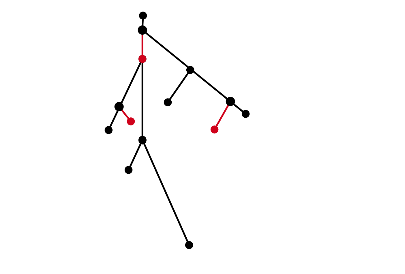
(f) Insertions in red.

Figure 2: (b)$\rightarrow$(e) form an edit path made from the left weighted tree in Figure 2(a) to the right one. Each time the edges involved in the editing are highlighted with different colors. In the following plot such vertices return black. This edit path can clearly be represented with a mapping - Section 4.2 - made by couples $(v,"D")$ for all the red vertices in Figure 2(b), $(v,"G")$ for all the yellow vertices in Figure 2(c), $(v,w)$ for all the vertices associated via the green color in Figure 2(d), $("G",w)$ for all the yellow vertices in Figure 2(c) and $("D",w)$ for all the red vertices in Figure 2(f).

The set of all weighted trees considered up to ghostings and splittings is called $(\mathcal{T}_{2},\mathbb{R}_{\geq 0})$.

A weighted tree $T$ can be edited to obtain another weighted tree, on which one can apply a new edit to obtain a third tree and so on. Any finite composition of edits is called edit path. See Figure 2 for an example of an edit path. The set of finite edit paths between $T$ and $T^{\prime}$ is called $\gamma\in\Gamma(T,T^{\prime})$.

The cost of the edit operations is defined as follows:

• the cost of shrinking an edge is equal to the absolute value of the difference of the two weights;

• for any deletion/insertion, the cost is equal to the weight of the edge deleted/inserted;

• the cost of ghosting is zero.

The cost of an edit path is the sum of the costs of its edit operations. Putting all the pieces together, the edit distance $d_{E}$ between weighted trees is defined as:

$$d_{E}(T,T^{\prime})=\inf_{\gamma\in\Gamma(T,T^{\prime})}cost(\gamma)$$

where $\Gamma(T,T^{\prime})$ indicates the set of edit paths which start in $T$ and end in $T^{\prime}$. In Pegoraro (2021b) it is proved that $d_{E}$ is a metric on the space of weighted trees considered up to order two vertices.

Remark 2

It would be natural to try to define a family of metrics indexed by integers $p\geq 1$ by saying that the costs of an edit path the $p$-th root of sum of the costs of the edit operations to the $p$-th power. But now we can easily see that for any $p>1$ this has no hope of being a meaningful pseudo metric for weighted trees. In fact, consider the case of a weighted tree made by two vertices and one edge with weight $1$. The cost of shrinking the $p$-metric would be $\parallel 1\parallel_{p}=1$. At the same time one can split it in half with $0$ cost and the cost of shrinking this other tree would be $\parallel(1/2,1/2)\parallel_{p}<1$. Splitting the segment again and again will make its shrinking cost go to $0$. In other words all weighted trees, if considered up to order $2$ vertices, would be at distance zero from the tree with no branches.

4.2 Mappings

Given an edit path between two weighted trees, its cost is often invariant up to many permutations of the edits. To better work in such environment, we start considering paths up to some permutation of the edits. Objects called mappings, as defined in Pegoraro (2023), help us in doing this, as well as making the metric $d_{E}$ more tractable. For this reason now we report their definition. As in Pegoraro (2023), $"D"$ and $"G"$ are be used to indicate “deletion” and “ghosting”. Some novel notation is established and it is highlighted via 3 to help the reader.

A mapping between $T$ and $T^{\prime}$ is a set $M\subset(E_{T}\cup\{"D","G"\})\times(E_{T^{\prime}}\cup\{"D","G"\})$ satisfying:

• consider the projection of the Cartesian product $(E_{T}\cup\{"D","G"\})\times(E_{T^{\prime}}\cup\{"D","G"\})\rightarrow(E_{T}\cup\{"D","G"\})$; we can restrict this map to $M$ obtaining $\pi_{T}:M\rightarrow(E_{T}\cup\{"D","G"\})$. The maps $\pi_{T}$ and $\pi_{T^{\prime}}$ are surjective on $E_{T}\subset(E_{T}\cup\{"D","G"\})$ and $E_{T^{\prime}}\subset(E_{T^{\prime}}\cup\{"D","G"\})$ respectively;

• $\pi_{T}$ and $\pi_{T^{\prime}}$ are injective;

• $M\cap(V_{T}\times V_{T^{\prime}})$ is such that, given $(a,b)$ and $(c,d)\in M\cap(V_{T}\times V_{T^{\prime}})$, $a>c$, if and only if $b>d$;

• if $(a,"G")$ (or $("G",a)$) is in $M$, let $child(a)=\{b_{1},..,b_{n}\}$. Then there is one and only one $i$ such that for all $j\neq i$, for all $x\in V_{sub(b_{j})}$, we have $(x,"D")\in M$ (respectively $("D",x)$); and there is one and only one $c$ such that $c=\max\{x^{\prime}\in sub(b_{i})\mid(x^{\prime},y)\in M$ for any $y\in V_{T^{\prime}}\}$. In other words, if $(a,"G")\in M$, then $a$ becomes an order $2$ vertex after applying all the deletions induced by $(b,"D")\in M$.

We call $\operatorname*{Mapp}(T,T^{\prime})$ the set of all mappings between $T$ and $T^{\prime}$.

As in Pegoraro (2023), we use the properties of $M\in\operatorname*{Mapp}(T,T^{\prime})$ to parametrize a set of edit paths starting from $T$ and ending in $T^{\prime}$, which are collected under the name $\gamma_{M}$.

• $\gamma_{d}^{T}$ a path made by the deletions to be done in $T$, that is, the couples $(v,"D")$, executed in any order. So we obtain $T^{M}_{d}=\gamma_{d}^{T}(T)$, which, instead, is well defined and not depending on the order of the deletions.

• One then proceeds with ghosting all the vertices $(v,"G")$ in $M$, in any order, getting a path $\gamma^{T}_{g}$ and the dendrogram $T_{M}:=\gamma^{T}_{g}\circ\gamma^{T}_{d}(T)$.

• Since all the remaining points in $M$ are couples, the two dendrograms $T^{\prime}_{M}$ (defined in the same way as $T_{M}$, but starting from $T^{\prime}$) and $T_{M}$ must be isomorphic as tree structures. This is guaranteed by the properties of $M$. So one can shrink $T_{M}$ onto $T^{\prime}_{M}$, and the composition of the shrinkings, executed in any order is an edit path $\gamma_{s}^{T}$.

By definition:

$$\gamma_{s}^{T}\circ\gamma_{g}^{T}\circ\gamma_{d}^{T}(T)=T^{\prime}_{M},$$

and:

$$(\gamma_{d}^{T^{\prime}})^{-1}\circ(\gamma_{g}^{T^{\prime}})^{-1}\circ\gamma_{s}^{T}\circ\gamma_{g}^{T}\circ\gamma_{d}^{T}(T)=T^{\prime}$$

.

where the inverse of an edit path is thought as the composition of the inverses of the single edit operations, taken in the inverse order.

Lastly, we call $\gamma_{M}$ the set of all possible edit paths of the form:

$$(\gamma_{d}^{T^{\prime}})^{-1}\circ(\gamma_{g}^{T^{\prime}})^{-1}\circ\gamma_{s}^{T}\circ\gamma_{g}^{T}\circ\gamma_{d}^{T}.$$

obtained by changing the order in which the edit operations are executed inside $\gamma_{d}$, $\gamma_{g}$ and $\gamma_{s}$. Observe that, even if $\gamma_{M}$ is a set of paths, its cost is well defined:

$$cost(M):=cost(\gamma_{M})=cost(\gamma_{d}^{T})+cost(\gamma_{s}^{T})+cost(\gamma_{d}^{T^{\prime}}).$$

Remark 3

For notational convenience, we collect in $M_{D}$ all the deletions of $M$, in $M_{G}$ all the ghostings and in $C(M)$ all the shrinking edits.

See Figure 2 for an example of a mapping between weighted trees. We conclude this section by recalling that Pegoraro (2021b) proves that given two weighted trees $T$ and $T^{\prime}$, for every finite edit path $\gamma\in\Gamma(T,T^{\prime})$, there exists a mapping $M\in\operatorname*{Mapp}(T,T^{\prime})$ such that $cost(M)\leq cost(\gamma)$.

Lastly, consider $M_{2}(T,T^{\prime})\subset\operatorname*{Mapp}(T,T^{\prime})$ defined as follows.

Definition 18 (Pegoraro (2023))

A mapping $M\in\operatorname*{Mapp}(T,T^{\prime})$ has maximal ghostings if $(v,"G")\in M$ if and only if $v$ is of order $2$ after the deletions in $T$ and, similarly $("G",w)\in M$ if and only if $w$ is of order $2$ after the deletions in $T^{\prime}$.

A mapping $M\in\operatorname*{Mapp}(T,T^{\prime})$ has minimal deletions if $(v,"D")\in M$ only if neither $v$ nor $father(v)$ are of order $2$ after applying all the other deletions in $T$ and, similarly, $("D",w)\in M$ only if $w$ is not of order $2$ after applying all the other deletions in $T^{\prime}$.

We collect all mappings with maximal ghostings and minimal deletions in the set $M_{2}(T,T^{\prime})$.

Lemma 1 (Pegoraro (2023))

$$\min\{cost(M)\mid M\in\operatorname*{Mapp}(T,T^{\prime})\}=\min\{cost(M)\mid M\in M_{2}(T,T^{\prime})\}$$

5 Merge Trees Edit Distance

In this section we finally exploit the notation established in the previous sections and results obtained in Pegoraro (2021b) to obtain a (pseudo) metric for merge trees.

5.1 Truncating Merge Trees

The aim of this section is to bridge between merge trees and weighted trees, in order to induce a metric on merge trees by means of the edit distance defined in Section 4. the general idea is that we want to truncate the edge going to infinity of a merge tree to obtain a weighted tree. Clearly, many details need to be taken care of, as the metric needs to be well defined and the practical consequences of any truncation process need to be formally addressed.

Starting from a merge tree $(T,h_{T})$ it is quite natural to turn the height function $h_{T}$ into a weight function $w_{T}$ via the rule $w_{T}((v,v^{\prime})):=h_{T}(v^{\prime})-h_{T}(v)$. The monotonicity of $h_{T}$ guarantees that $w_{T}$ take values in $\mathbb{R}_{>0}$. However, we clearly have an issue with the edge $(v,r_{T})$ as $h_{T}(r_{T})=+\infty$. To solve this issue we need some novel tools - see Figure 3. First consider the set of merge trees $\mathcal{MT}$ and build the subset $\mathcal{MT}_{K}:=\{(T,h_{T})\in\mathcal{MT}\mid\max h_{T}\leq K\}$, for some $K\in\mathbb{R}$. Then define the truncation operator as follows:

$$\textstyle\operatorname*{Tr}_{K}: \mathcal{MT}_{K}\xrightarrow{\hskip 56.9055pt}(\mathcal{T},\mathbb{R}_{\geq 0})$$ (1)

$$(T,h_{T})\mapsto(T,h_{K})\mapsto(T,w_{T})$$

with $h_{K}(v)=h_{T}(v)$ if $v<r_{T}$ and $h_{K}(r_{T})=K$. Then we set $w_{T}((v,v^{\prime}))=h_{K}(v^{\prime})-h_{K}(v)$. To avoid $w_{T}((v,r_{T}))=0$, if $\max h_{T}=K$, we take $(T,h_{T})\mapsto(T^{\prime},h_{T^{\prime}})\mapsto(T^{\prime},w_{T^{\prime}})$ with $T^{\prime}$ obtained from $T$ via the removal of $r_{T}$ from $V_{T}$ and $(v,r_{T})$ from $E_{T}$. The map $h_{T^{\prime}}$ is $h_{T\mid V_{T^{\prime}}}$. Then $w_{T^{\prime}}((v,v^{\prime})):=h_{T^{\prime}}(v^{\prime})-h_{T^{\prime}}(v)$.

In other words with $\operatorname*{Tr}_{K}$ we are fixing some height $K$, truncating the edge $(\arg\max h_{T},r_{T})$ at height $K$, and then obtaining a positively weighted tree, as in Figure 3. To go back with $(\operatorname*{Tr}_{K})^{-1}$ we “hang” a weighted tree at height $K$ and extend the edge $(v,r_{T})$ to $+\infty$. We formally state these ideas in the following proposition. We leave the details of the proof to the reader.

Proposition 3

The operator $\operatorname*{Tr}_{K}:\mathcal{MT}_{K}\rightarrow(\mathcal{T},\mathbb{R}_{\geq 0})$ can be inverted via $(T,w_{T})\mapsto\operatorname*{Tr}_{K}^{-1}((T,w_{T}))=(T^{\prime},h_{T^{\prime}})$ with the following notation: the tree structure $T^{\prime}$ is obtained from $T$ via adding $r_{T^{\prime}}$ to $V_{T}$ and $(r_{T},r_{T^{\prime}})$ to $E_{T}$ and ghosting $r_{T}$ if it becomes an order $2$ vertex. Then we have $h_{T^{\prime}}(r_{T})=K$ (if it is not ghosted, i.e. if it is of order greater than $2$), $h_{T^{\prime}}(r_{T^{\prime}})=+\infty$ and, recursively, for $(v,v^{\prime})\in E_{T}$, $h_{T^{\prime}}(v)=h_{T^{\prime}}(v^{\prime})-w_{T}((v,v^{\prime}))$. Clearly $\operatorname*{Tr}_{K}^{-1}(\operatorname*{Tr}_{K}((T,h_{T})))\cong(T,h_{T})$. Thus $\mathcal{MT}_{K}\cong(\mathcal{T},\mathbb{R}_{\geq 0})$ as sets, for every $K\in\mathbb{R}$. Moreover $\operatorname*{Tr}_{K}((T,h_{T}))\sim_{2}\operatorname*{Tr}_{K}((T^{\prime},h_{T^{\prime}}))$ if and only if $(T,h_{T})\sim_{2}(T^{\prime},h_{T^{\prime}})$.

(a) Two merge trees $T$ and $T^{\prime}$.

(b) A graphical representation of the weighted trees $\operatorname*{Tr}_{K}(T)$ and $\operatorname*{Tr}_{K}(T^{\prime})$. Roughly speaking, the merge trees $T$ and $T^{\prime}$ are recovered sending the two roots back to infinity.

Figure 3: A graphical representation of the truncation operator.

5.2 Edit Distance For Merge Trees

Consider $(T,h_{T}),(T^{\prime},h_{T^{\prime}})\in\mathcal{MT}$ and select $K$ such that $(T,h_{T}),(T^{\prime},h_{T^{\prime}})\in\mathcal{MT}_{K}$. Let $(G,w_{G})=\operatorname*{Tr}_{K}((T,h_{T}))$ and $(G^{\prime},w_{G^{\prime}})=\operatorname*{Tr}_{K}((T^{\prime},h_{T^{\prime}}))$. Lastly, set:

$$d_{K}((T,h_{T}),(T^{\prime},h_{T^{\prime}})):=d_{E}((G,w_{G}),(G^{\prime},w_{G^{\prime}})).$$

Despite being a promising and natural pseudo metric, $d_{K}$ is not defined on the whole $\mathcal{MT}$ and, on top of that, it is not clear if its value depends on the $K$ we choose. Leveraging on the following result taken from Pegoraro (2021b) we solve these issues and prove that we can use $d_{K}$ to define a metric on $\mathcal{MT}$.

Proposition 4 (Pegoraro (2021b))

Take $(T,w_{T})$ and $(T^{\prime},w_{T^{\prime}})$. If $r_{T}$ and $r_{T^{\prime}}$ are of order $1$ and there is a splitting $\{(v,r_{T})\}\rightarrow\{(v,v^{\prime}),(v^{\prime},r_{T})\}$ and $\{(w,r_{T^{\prime}})\}\rightarrow\{(w,w^{\prime}),(w^{\prime},r_{T^{\prime}})\}$ giving the weighted trees $(G,h_{G})$ and $(G^{\prime},h_{G^{\prime}})$, such that: $w_{G}((v^{\prime},r_{T}))=w_{G^{\prime}}((w^{\prime},r_{G}))$, then $d_{E}(T,T^{\prime})=d_{E}(sub_{G}(v^{\prime}),sub_{G^{\prime}}(w^{\prime}))$.

Thus we define the edit distance between merge trees as follows.

Theorem 1 (Merge Tree Edit Distance)

Given two merge trees $(T,h_{T}),(T^{\prime},h_{T^{\prime}})$ such that $(T,h_{T}),(T^{\prime},h_{T^{\prime}})\in\mathcal{MT}_{K}$ and $(T,h_{T}),(T^{\prime},h_{T^{\prime}})\in\mathcal{MT}_{K^{\prime}}$, then $d_{K}(T,T^{\prime})=d_{K^{\prime}}(T,T^{\prime})$.

Thus, for any couple of merge trees in $\mathcal{MT}$, we can define the merge tree edit distance

$$d_{E}((T,h_{T}),(T^{\prime},h_{T^{\prime}})):=d_{K}((T,h_{T}),(T^{\prime},h_{T^{\prime}}))$$

for any $K\geq\max\{\max h_{T},\max h_{T^{\prime}}\}$.

By 3 we also have the following corollary of 1.

Corollary 1

The distance $d_{E}$ is a pseudo metric on $\mathcal{MT}$ and a metric on $\mathcal{MT}/\sim_{2}$: given two merge trees $(T,h_{T})$ and $(T^{\prime},h_{T^{\prime}})$, $d_{E}((T,h_{T}),(T^{\prime},h_{T^{\prime}}))=0$ if and only if $(T,h_{T})\sim_{2}(T^{\prime},h_{T^{\prime}})$ if and only if (by 1) $\mathcal{F}((T,h_{T}))\cong\mathcal{F}((T^{\prime},h_{T^{\prime}}))$.

Remark 4

1 and 1 have a series of important implications. First, they say that $(\mathcal{MT}_{K}/\sim_{2},d_{E})$ is isometric and isomorphic to $(\mathcal{T}_{2},d_{E})$ and thus, if we have a subset of merge trees contained in $\mathcal{MT}_{K}/\sim_{2}$, for some $K$, we can map them in $(\mathcal{T}_{2},d_{E})$ via $\operatorname*{Tr}_{K}$ and carry out our analysis there. Second, suppose we are given a merge tree $T^{\prime\prime}$ with $\max h_{T^{\prime\prime}}>K$. For any two merge trees $T,T^{\prime}$ with $K\geq\max h_{T},\max h_{T^{\prime}}$, we can consider $K^{\prime}\geq\max h_{T^{\prime\prime}}$ and compute $d_{E}(T,T^{\prime\prime})=d_{K^{\prime}}(T,T^{\prime\prime})$ and $d_{E}(T^{\prime},T^{\prime\prime})=d_{K^{\prime}}(T^{\prime},T^{\prime\prime})$. But we do not have to compute again $d_{K^{\prime}}(T,T^{\prime})$ for we have $d_{E}(T,T^{\prime})=d_{K^{\prime}}(T,T^{\prime})=d_{K}(T,T^{\prime})$. Lastly, putting all the pieces together, the metric $d_{E}$ can be pulled back as a metric on regular abstract merge trees.

We close this section with the following remark.

Remark 5

A more naive approach could have been to model each merge tree as a triplet $(G,w_{G},h_{T}(v))\in(\mathcal{T},\mathbb{R}_{\geq 0})\times\mathbb{R}$, with $v=\arg\max h_{T}$ and $G=sub_{T}(v)$ - i.e. to record the height of the last merging point in $T$ and then remove $(v,r_{T})$ from $E_{T}$. Then one could define a pseudo metric on $\mathcal{MT}$ via the rule:

$$d((T,h_{T}),(T^{\prime},h_{T^{\prime}}))=\mid h_{T}(v)-h_{T^{\prime}}(v^{\prime})\mid+d_{E}((G,w_{G}),(G^{\prime},w_{G^{\prime}})).$$

but this leads to unpleasant and unstable behaviours, as in Figure 4. Such behaviours do not appear with the definition we have given.

Assumption 2

Coherently with 1 and 4, to avoid overloading the notation, from now on always assume that we have fixed $K$ big enough for our purposes. For instance, when we take a merge tree $(T,h_{T})$ we always imply that we have fixed $K>\max h_{T}$ so that we can indicate with $(T,w_{T})$ the weighted tree $\operatorname*{Tr}_{K}((T,h_{T}))$.

(a) Two merge trees $T$ (left) and $T^{\prime}$ (right).

(b) The two merge trees $T$ (left) and $T^{\prime}$ (right) in Figure 4(a) represented as triplets of the form $(G,w_{G},h_{T}(v))$ - see 5. The shaded red edges represent the merge trees $T$ and $T^{\prime}$, which are removed to obtained the weighted trees. The height values $h_{T}(v)$ are colored in red. The red edges represent deletions and the green arrows couple the remaining edges, giving a mapping. The cost of such mapping is given by the height differences $\mid h_{T}(v)-h_{T^{\prime}}(f^{\prime})\mid$ plus the two deletions and the weight differences between the coupled edges (which visually appear to be very small). Clearly such distance is inflated by having to account both for $\mid h_{T}(v)-h_{T^{\prime}}(f^{\prime})\mid$ and for the deletion of $(v^{\prime},f^{\prime})$.

(c) The weighted trees $\operatorname*{Tr}_{K}(T)$ (left) and $\operatorname*{Tr}_{K}(T^{\prime})$ (right) with $K=t^{\prime}_{3}$, obtained from the merge trees $T$ and $T^{\prime}$ as in Figure 4(a). The red edges represent deletions and the green arrows couple the remaining edges, giving a mapping. The cost of such mapping is given by the weight differences between the coupled edges. Note that the weight difference between $(v,r_{T})$ and $(v^{\prime},r_{T^{\prime}})$ - i.e. $h_{T}(v)-h_{T^{\prime}}(v^{\prime})$ - is surely smaller than the cost of deleting $(v^{\prime},f^{\prime})$

.

Figure 4: A situation in which the metric defined in 5 shows an unnatural behaviour, while $d_{K}$ still behaves naturally.

5.3 Stability

Merge trees are trees which are used to represent data and, considering populations of such objects, to explore the variability of a data set. Thus, any metric which is employed on merge trees (and on any data representation in general) needs to measure the variability between merge trees in a “sensible” way, coherently with the application considered. A formal way to assess such properties comes often in the form of continuity results of the operator mapping data into representations, which, in TDA’s literature, are usually referred to as stability results. The study of the stability properties of $d_{E}$ is carried out in Pegoraro and Secchi (2021), where merge trees are used to tackle a functional data analysis problem. In this section we report such result and comment on it.

Stability results are usually understood in terms of interleavings between persistence modules (Chazal et al., 2008): the distance one measures between (a summary of) the persistence modules should not deviate too much from the interleaving distance between the modules themselves. The rationale behind these ideas follows from the fact that given two functions $f,g:X\rightarrow\mathbb{R}$ with suitable properties and such that $\parallel f-g\parallel_{\infty}<\varepsilon$, then their sublevel set filtrations induce $\varepsilon$-interleaved persistence modules via homology functors. Moreover, interleaving distances are taken as reference because they are universal among the metrics bounded from above by $\parallel f-g\parallel_{\infty}$ (Lesnick, 2015; Cardona et al., 2021): for any other metric $d$ on persistence modules/multidimensional persistence modules/merge trees such that $d(S_{f},S_{g})\leq\parallel f-g\parallel_{\infty}$ then $d(S_{f},S_{g})\leq d_{I}(S_{f},S_{g})$, with $S_{f},S_{g}$ being the persistence modules/multidimensional persistence modules/merge trees representing $f,g$ and $d_{I}$ being the interleaving distance between them. Thus a good behaviour in terms of interleaving distance implies a good handling of pointwise noise between functions and so also interpretability of the metric.

For this reason we report the following definitions, which are originally stated by Morozov et al. (2013) with a different notation.

Definition 19 (adapted from Morozov et al. (2013))

Given $X_{\operatorname*{\scalerel*{\cdot}{\bigodot}}}$ filtration and $\varepsilon>0$, we define $X_{\operatorname*{\scalerel*{\cdot}{\bigodot}}}^{\varepsilon}$ as $X_{t}^{\varepsilon}:=X_{t+\varepsilon}$ and $X_{t\leq t^{\prime}}^{\varepsilon}:=X_{t+\varepsilon\leq t^{\prime}+\varepsilon}$.

Consider two abstract merge trees $\pi_{0}(X_{\operatorname*{\scalerel*{\cdot}{\bigodot}}})$ and $\pi_{0}(Y_{\operatorname*{\scalerel*{\cdot}{\bigodot}}})$. Two natural transformations $\alpha:\pi_{0}(X_{\operatorname*{\scalerel*{\cdot}{\bigodot}}})\rightarrow\pi_{0}(Y_{\operatorname*{\scalerel*{\cdot}{\bigodot}}}^{\varepsilon})$ and $\beta:\pi_{0}(Y_{\operatorname*{\scalerel*{\cdot}{\bigodot}}})\rightarrow\pi_{0}(X_{\operatorname*{\scalerel*{\cdot}{\bigodot}}}^{\varepsilon})$ are $\varepsilon$-compatible if:

• $\beta_{t+\varepsilon}\circ\alpha_{t}=\pi_{0}(X_{t\leq t+2\varepsilon})$

• $\alpha_{t+\varepsilon}\circ\beta_{t}=\pi_{0}(Y_{t\leq t+2\varepsilon})$.

Then, the interleaving distance between $T$ and $G$ is:

$$d_{I}(\pi_{0}(X_{\operatorname*{\scalerel*{\cdot}{\bigodot}}}),\pi_{0}(Y_{\operatorname*{\scalerel*{\cdot}{\bigodot}}}))=\inf\{\varepsilon>0\mid\exists\alpha,\beta\text{ }\varepsilon-\text{compatible}\}.$$

We also say that $\pi_{0}(X_{\operatorname*{\scalerel*{\cdot}{\bigodot}}})$ and $\pi_{0}(Y_{\operatorname*{\scalerel*{\cdot}{\bigodot}}})$ are $d_{I}(\pi_{0}(X_{\operatorname*{\scalerel*{\cdot}{\bigodot}}}),\pi_{0}(Y_{\operatorname*{\scalerel*{\cdot}{\bigodot}}}))$-interleaved.

Being the edit distance a summation of the costs of local modification of trees we expect that $d_{E}$ cannot be bounded from above by the interleaving distance between merge trees as is the case, for instance, with the bottleneck distance between persistence diagrams (Morozov et al., 2013): such metric in fact is defined as the biggest modification ones needs to optimally match two persistence diagrams. To better formalize this, we prove the following result. For a more detailed comparison between these two (and other) metrics for merge trees see also Section B.

Proposition 5

We always have $d_{I}(T,G)\leq d_{E}(T,G)$.

Thus, a suitable stability condition would be for the edit distance to be dependent on the number of vertices in the merge trees but, at the same time, that the cost of the local modifications we need to match the two merge trees goes to $0$ as their interleaving distance get smaller and smaller.

Definition 20 (Pegoraro (2021b))

Given a constructible persistence module $S:\mathbb{R}\rightarrow\operatorname*{Vec}_{\mathbb{K}}$, we define its rank as $\operatorname*{rank}(S):=\#PD(S)$ i.e. the number of points in its persistence diagram. When $S$ is generated on $\mathbb{K}$ by a regular abstract merge tree $\pi_{0}(X_{\operatorname*{\scalerel*{\cdot}{\bigodot}}})$ we have $\operatorname*{rank}(S):=\#PD(S)=\#L_{T}$, with $(T,h_{T})=\mathcal{M}(\pi_{0}(X_{\operatorname*{\scalerel*{\cdot}{\bigodot}}}))$ and may refer to $\operatorname*{rank}(S)$ also as the rank of the merge tree $\operatorname*{rank}(T)$. We also fix the notation $\dim(T):=\#E_{T}$.

Definition 21

Given $\pi_{0}(X_{\operatorname*{\scalerel*{\cdot}{\bigodot}}})$ and $\pi_{0}(Y_{\operatorname*{\scalerel*{\cdot}{\bigodot}}})$ $\varepsilon$-interleaved abstract merge trees; a metric for merge trees is locally stable if:

$$d(T,T^{\prime})\leq C(\operatorname*{rank}(T)+\operatorname*{rank}(T^{\prime}))\varepsilon$$

for some $C>0$.

In view of this definitions we can rewrite the following theorem from Pegoraro and Secchi (2021) and obtain the local stability as an easy corollary.

Theorem 2 (Pegoraro and Secchi (2021))

If there are $\alpha,\beta$ $\varepsilon$-compatible maps between two abstract merge trees trees $\pi_{0}(X_{\operatorname*{\scalerel*{\cdot}{\bigodot}}}),\pi_{0}(Y_{\operatorname*{\scalerel*{\cdot}{\bigodot}}})$, then there exist a mapping $M$ between $T=\mathcal{M}(\pi_{0}(X_{\operatorname*{\scalerel*{\cdot}{\bigodot}}}))$ and $G=\mathcal{M}(\pi_{0}(Y_{\operatorname*{\scalerel*{\cdot}{\bigodot}}}))$ such that $cost_{M}((a,b))\leq 2\varepsilon$ for every $(a,b)\in M$.

Corollary 2

Since for a merge tree $(T,h_{T})$ we have $\#V_{T}\leq 2\#L_{T}$ and $\operatorname*{rank}(T)=\#L_{T}$, then $d_{E}$ is locally stable.

6 The geometry of $(\mathcal{MT},d_{E})$

Now we start the investigation of the metric space of merge trees. The structures that we are going to build up throughout the section can all be seen in Figure 5 and Figure 6.

As already stated in the Introduction, this investigation has the general goal of understanding, at least partially, the local geometry of the metric space $(\mathcal{MT},d_{E})$. To achieve this goal, we stratify merge trees according to their dimension and explore the behaviour of the space along these strata and across these strata. As a first result, the topological properties which are obtained in terms of within-in strata completeness and compactness lead to the existence of Frechét Means, which are very important objects for non-Euclidean statistics (see Section 6.5). On the other hand, the decomposition of geodesic paths along different strata leads to the local parametrization result in Section 6.7. Such result is very promising in terms of the development of statistical techniques like regression and principal components analysis and immediately leads to a simple approximation scheme for Frechét Means - whose properties are not assessed in the present work. Clearly, the picture is far from being complete and many questions remain open: for instance the possibility of doing differential calculus in the space of merge trees or retrieving more global information like the quantification - in some measure-related terms - of the well-behaved trees still need to be studied.

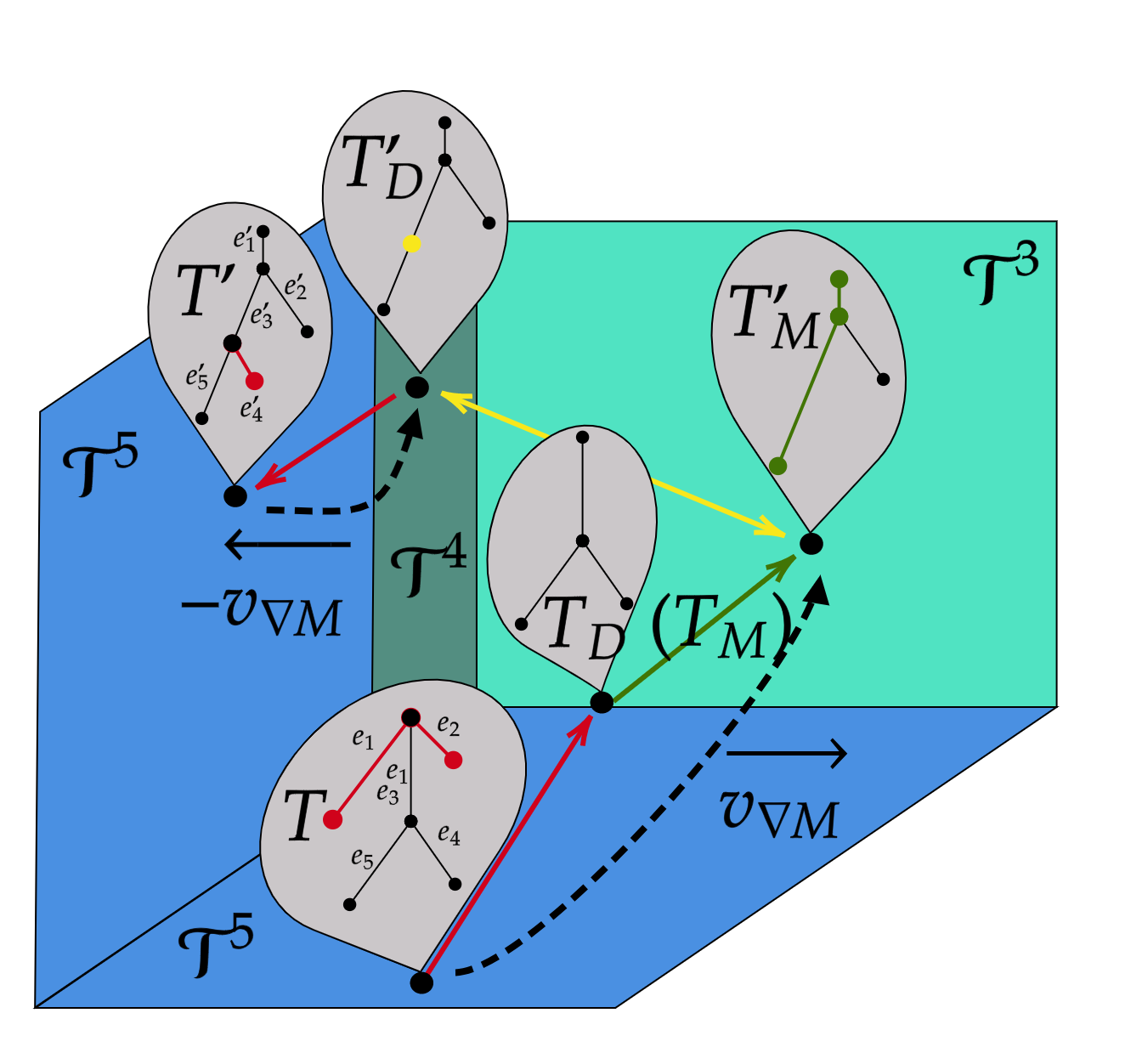
Figure 5: A mapping $M$ with the associated geodesic and the dashed arrows which represent the $\left(T\xrightarrow{\hskip 1.42271pt}T^{\prime}\right)$-decomposition via the canonical representation of $M$ (see Section 6.7): starting from $T$, the red arrow ending in $T_{D}$ (which is equal to $T_{M}$) represents the deletion of $e_{1}$ and $e_{2}$, the following green arrow shrinks the green edges $e_{3}$ and $e_{5}$ to obtain $T^{\prime}_{M}$, the yellow double headed arrow is a length $0$ jump between the two trees $T^{\prime}_{D}\leq T^{\prime}_{M}$, which are equal up to the splitting induced by the yellow vertex and then the red arrow pointing in $T^{\prime}$ represents the insertion of the red edge $e^{\prime}_{4}$. The vector $\overrightarrow{v_{\nabla M}}$ represents the geodesic paths from $T$ for $T^{\prime}_{M}$ and thus is given by: $-w_{T}(e_{1})\bm{e_{1}}-w_{T}(e_{2})\bm{e_{2}}-a\bm{e_{3}}+0\bm{e_{4}}+b\bm{e_{5}}=(-w_{T}(e_{1}),-w_{T}(e_{2}),-a,0,b)\in R^{T},$ with $a,b>0$ which give the shrinking that ends in $T^{\prime}_{M}$. The vector $\overleftarrow{v_{\nabla M}}$, instead, goes from $T^{\prime}$ to $T^{\prime}_{M}$ and accounts just for the deletion of $e^{\prime}_{4}$. The double headed yellow arrow then identifies $T_{M}$ and $T^{\prime}_{M}$ modulo order $2$ vertices. So $\overleftarrow{v_{\nabla M}}$ is given by $0\bm{e^{\prime}_{1}}+0\bm{e^{\prime}_{2}}+0\bm{e^{\prime}_{3}}-w_{T^{\prime}}(e^{\prime}_{4})\bm{e^{\prime}_{4}}+0\bm{e^{\prime}_{5}}=(0,0,0,-w_{T^{\prime}}(e^{\prime}_{4}),0)\in R^{T^{\prime}}$.

Figure 6: A qualitative and synthetic representation of the structures introduced in Section 6. All the tree are contained in $\mathcal{T}^{4}$, i.e. they have at most four edges. The two different shades of blue separates the trees in $\mathcal{T}^{3}$ - light blue, trees with $\leq 3$ edge - and the trees with $4$ edges - blue. Each tree is represented by a black dot in this space and can be visualized inside a grey cloud. In the left “page” of the blue surface we see a geodesic represented by a green arrow, which progressively shrinks an edge - the green one - up to deleting it and obtaining a tree in $\mathcal{T}^{3}\cap\mathcal{T}^{4}$. On the right “page”, instead, we see two trees joined by two optimal mappings: the one represented by the red arrows which deletes the red edge - and so goes through $\mathcal{T}^{3}\cap\mathcal{T}^{4}$ - and the regrows it swapping two children, and the green one which instead shrinks the two green edges with the direction given by the arrows. In the light blue region we see a weighted tree $T$ with a yellow open neighborhood which represents $B_{\mathcal{K}^{T}/2}(T)$ and is homeomorphic via $\log_{T}$ and $\exp_{T}$ to an open neighborhood of the origin in $\mathbb{R}^{T}_{>T}\subset\mathbb{R}^{3}$.

6.1 Merge Trees, Weighted Trees and Order 2 Vertices

Recall that $\mathcal{MT}$ is the space of merge trees up to isomorphism, $\mathcal{T}$ (abbreviation for $(\mathcal{T},\mathbb{R}_{\geq 0})$) is the space of weighted trees, $\mathcal{MT}/\sim_{2}$ and $\mathcal{T}_{2}$ are the respective quotient spaces for merge tree and weighted trees up to order $2$ vertices. Moreover, by Section 5.2, we have the isometry $(\mathcal{MT}_{K},d_{E})\cong(\mathcal{T},d_{E})$ for any $K\in\mathbb{R}$, with this isomorphism of metric spaces passing to $(\mathcal{MT}_{K}/\sim_{2},d_{E})\cong(\mathcal{T}_{2},d_{E})$.

Both for weighted trees and for merge trees we indicate with $T_{2}$ the only representative without order $2$ vertices inside the equivalence class of $T$; if needed in the discussion, we call such equivalence class $[T]$. We have already seen that $d_{E}(T,T^{\prime})=0$ iff $T\sim_{2}T^{\prime}$. This is equivalent to saying that, if we consider the topological spaces $(\mathcal{MT},d_{E})$ and $(\mathcal{MT}/\sim_{2},d_{E})$ (or $(\mathcal{T},d_{E})$ and $(\mathcal{T}_{2},d_{E})$), respectively with the pseudo-metric and the metric topology, then $(\mathcal{MT}/\sim_{2},d_{E})$ is the metric space induced by the pseudometric $d_{E}$ of $\mathcal{MT}$ via metric identification i.e. $x\sim y$ iff $d(x,y)=0$. In particular, the projection on the quotient $\Pi:\mathcal{MT}\rightarrow\mathcal{MT}/\sim_{2}$ preserves distances and so open balls. In other words we can focus our attention on $\mathcal{T}$ and $\mathcal{MT}$, to avoid formal complications given by equivalence classes, and most topological result obtained for such space will hold also for $\mathcal{T}_{2}$ and $\mathcal{MT}/\sim_{2}$. In particular, since $B_{\varepsilon}(T)=B_{\varepsilon}(T^{\prime})$ for any $T\sim_{2}T^{\prime}$ - recall that $B_{\varepsilon}(T)=\{T^{\prime}\big{|}d_{E}(T,T^{\prime})<\varepsilon\}$ - to obtain local topological results we can always assume $T=T_{2}$.

In a similar fashion we focus our attention on the space of weighted trees and then point out how to extend the results to merge trees via a suitable isometry $(\mathcal{MT}_{K},d_{E})\cong(\mathcal{T},d_{E})$. On top of that, we also exploit the following trivial fact.

Proposition 6

Given a merge tree $(T,h_{T})$ then for every $\varepsilon>0$ there is $K\in\mathbb{R}$ such that $B_{\varepsilon}(T)\subset\mathcal{MT}_{K}$.

6.2 Subspaces

To start things off, there is a natural notion of dimension for weighted trees, which we have already introduced and used. We have already defined $\dim(T)=\#E_{T}$, that is, the number of edges in the tree structure $T$. To induce a suitable notion of dimension in $\mathcal{T}_{2}$ we do as follows: $\dim([T])=\inf_{T^{\prime}\in[T]}\dim(T^{\prime})$, which entails $\dim([T])=\dim(T_{2})$.

We take the exact same definitions also for any merge tree $(T,h_{T})$. Note that $\dim(T)=\dim\operatorname*{Tr}_{K}(T)$ for any $K>\max h_{T}$.

Now we can consider trees grouped by dimension.

Definition 22

$\mathcal{T}^{N}=\{T|\dim(T)\leq N\}$ for any $N\in\mathbb{N}$. The subspaces $\mathcal{T}_{2}^{N}$, $\mathcal{MT}^{N}$ and $\mathcal{MT}^{N}/\sim_{2}$ are defined analogously.

Understanding how these strata interact with each other and how we can navigate between them can shed some light on the structure of these metric spaces.

6.3 From Edits to Geodesics

Thanks to the results in Pegoraro (2023) we know that there are always edit paths which attain the metric $d_{E}$ between two weighted trees.

Consider an optimal edit path $e_{n}\circ\ldots\circ e_{1}(T)=G$; now we show that it can be seen as the discretization of a continuous curve $\gamma:[0,1]\rightarrow\mathcal{T}$ at points $t_{j}=\sum_{i=1}^{j}cost(e_{i})/d_{E}(T,G)$. Set $t_{0}=0$.

Pick an edit $e_{i}$ and let $T^{\prime}$ be $T^{\prime}=e_{i-1}\circ\ldots\circ e_{1}(T)$. We have $d_{E}(T^{\prime},e_{i}(T^{\prime}))=cost(e_{i})$. Suppose $e_{i}$ is a deletion or the shrinking of an edge $e=(v,v^{\prime})$ and let $C$ be the weight of $e$ after $e_{i}$ or $C=0$ if $e_{i}$ is a deletion.

We define $\gamma_{i}:[t_{i-1},t_{i})\rightarrow\mathcal{T}$ as $\gamma_{i}(t)=T^{\prime}_{t}$ with $T^{\prime}_{t}\cong T^{\prime}$ as tree structures and

$$w_{T^{\prime}_{t}}(e)=w_{T^{\prime}}(e)+\frac{(t-t_{i-1})}{t_{i}-t_{i-1}}(C-w_{T^{\prime}}(e)).$$

Note that, for $t\in[t_{i-1},t_{i})$ and $\varepsilon>0$ such that $t_{i}+\varepsilon\in[t_{i-1},t_{i})$, we have:

$$d_{E}(\gamma_{i}(t),\gamma_{i}(t+\varepsilon))= \mid w_{T^{\prime}}(e)+\frac{(t-t_{i-1})}{t_{i}-t_{i-1}}(C-w_{T^{\prime}}(e))-(w_{T^{\prime}}(e)+\frac{(t+\varepsilon-t_{i-1})}{t_{i}-t_{i-1}}(C-w_{T^{\prime}}(e)))\mid$$

$$= \frac{\varepsilon}{t_{i}-t_{i-1}}\mid C-w_{T^{\prime}}(e)\mid.$$

Thus for every $t_{i-1}=t^{1}<\ldots<t^{m}=t_{i}$ we have:

$$\sum_{j=1}^{m-1}d_{E}(\gamma_{i}(t^{j}),\gamma_{i}(t^{j+1}))\mid C-w_{T^{\prime}}(e)\mid=\sum_{j=1}^{m-1}\frac{t^{j+1}-t_{j}}{t_{i}-t_{i-1}}\mid C-w_{T^{\prime}}(e)\mid=\mid C-w_{T^{\prime}}(e)\mid=cost(e_{i})$$

As a consequence, the length of $\gamma_{i}$ is $cost(e_{i})$. Moreover we can define $\gamma_{i}(1)=T^{\prime}$. Note that $\gamma_{i}$ is continuous. If instead of $e_{i}$ being a deletion we consider an insertion, we define $\gamma_{i}(t)=\gamma^{\prime}_{i}(1-t)$ with $\gamma^{\prime}_{i}$ being obtained from the deletion $e_{i}^{-1}$. Lastly, if $e_{i}$ is a ghosting we define $\gamma_{i}(t)=e_{i}(T^{\prime})$ for all $t\in[t_{i-1},t_{i}]$. In this case the length of $\gamma_{i}$ is $0$.

Thus let $\gamma:[0,1]\rightarrow\mathcal{T}$ be $\gamma_{n}\circ\ldots\gamma_{1}$. Note that:

$$t_{i}-t_{i-1}=\sum_{j=1}^{i}cost(e_{j})/d_{E}(T,G)-\sum_{j=1}^{j-1}cost(e_{j})/d_{E}(T,G)=cost(e_{i})/d_{E}(T,G)$$

Consider now $t<t^{\prime}\in[0,1]$. If $t,t^{\prime}\in[t_{i-1},t_{i}]$ we have

$$d_{E}(\gamma(t),\gamma(t^{\prime}))=\frac{t^{\prime}-t}{t_{i}-t_{i-1}}cost(e_{i})=(t^{\prime}-t)d_{E}(T,G).$$

If instead $t\in[t_{i-1},t_{i}]$ and $t^{\prime}\in[t_{j-1},t_{j}]$, with $i<j$, we have:

$$d_{E}(\gamma(t),\gamma(t^{\prime}))= d_{E}(\gamma(t),\gamma(t_{i}))+d_{E}(\gamma(t_{j-1}),\gamma(t^{\prime}))+\sum_{k=i}^{j-1}d_{E}(\gamma(t_{k}),\gamma(t_{k+1}))$$

$$= d_{E}(T,G)\left(t_{i}-t+\sum_{k=i}^{j-1}t_{k+1}-t_{k}+t^{\prime}-t_{j-1}\right)=d_{E}(T,G)\left(t^{\prime}-t\right).$$

Thus $\gamma$ is a minimizing geodesic, as in 15 and, moreover, it induces a geodesic in the quotient under $\sim_{2}$. Note that if we have $(T,h_{T})$ and $(G,h_{G})$ merge trees, then embedding them in the in the space of weighted trees, we can obtain the same results. From now on, with an abuse of notation, with the term geodesic we indicate either a minimal edit path or the curve obtained from the minimal edit path as explained above.

Pegoraro (2023), shows that for any pair of weighted trees the distance between them is given by the length of a path $\gamma_{M}$, with $M$ being a mapping between the two trees. Moreover, looking at how mappings parametrize finite edit paths, we see that if $T,T^{\prime}\in\mathcal{T}^{N}$, then there is at least a geodesic between them which does not exit $\mathcal{T}^{N}$. By considering $T_{2}$ and $T^{\prime}_{2}$ we obtain the same consequence for $\mathcal{T}_{2}^{N}$. Clearly all these things hold true also for merge tree, via isometries. We sum up these facts with the following proposition.

Proposition 7

The spaces $(\mathcal{T},d_{E})$, $(\mathcal{T}_{2},d_{E})$, $(\mathcal{T}^{N},d_{E})$, $(\mathcal{T}_{2}^{N},d_{E})$, $(\mathcal{MT},d_{E})$, $(\mathcal{MT}/\sim_{2},d_{E})$, $(\mathcal{MT}^{N},d_{E})$ and $(\mathcal{MT}^{N}/\sim_{2},d_{E})$ are geodesic spaces.

6.4 Topology

Topology plays a central role when investigating the properties of a space. For instance, being able to characterize or identify open, closed and in particular compact sets is fundamental to work with real valued operators defined on such space. Thanks to 5, we have already seen that the topology induced by $d_{E}$ is richer than the one induced by $d_{I}$ as, for any $T^{\prime}\in\mathcal{MT}$ and $C>0$, the following hold:

$$\{T\in\mathcal{MT}\mid d_{E}(T,T^{\prime})<C\}\subset\{T\in\mathcal{MT}\mid d_{I}(T,T^{\prime})<C\}.$$

Note that the topology induced by $d_{E}$ is strictly bigger than the one induced by $d_{I}$: it is not difficult to build a tree $T$ and a sequence $\{T_{n}\}_{n\in\mathbb{N}}$ such that $d_{I}(T_{n},T)\rightarrow 0$ and $d_{E}(T_{n},T)\rightarrow+\infty$. For instance let $T$ be a merge tree with just one edge and obtain $T_{n}$ by attaching to such edge $n^{2}$ edges of length $2/n$: $d_{I}(T,T_{n})=1/n$, while $d_{E}(T,T_{n})=2n$. This implies that, in general, $d_{E}$ is potentially better than $d_{I}$ at separating trees in data analysis applications, tough it is more sensitive to noise.

We establish the following notation for weighted trees: $\parallel T\parallel=\sum_{e\in E_{T}}w_{T}(e)$, so that the reversed triangle inequality in the case of weighted trees has the following form.

Proposition 8

Given $T$, $T^{\prime}$ weighted trees, we have:

$$\mid\parallel T\parallel-\parallel T^{\prime}\parallel\mid\leq d_{E}(T,T^{\prime})$$

If we have two weighted trees $T\sim_{2}T^{\prime}$, then $\parallel T\parallel=\parallel T^{\prime}\parallel$ and thus 8 holds also in $\mathcal{T}_{2}$. Instead $\parallel T\parallel$ is not well defined for merge trees as it depends on the embedding $\operatorname*{Tr}_{K}$.

Given $C>0$, we have $B(C):=B_{C}(\{\star\})=\{T\in\mathcal{T}\mid\parallel T\parallel<C\}$. We also establish the notation: $B(C)^{N}:=B(C)\bigcap\mathcal{T}^{N}$.

The following result presents some topological properties of the space $\mathcal{T}$ and its subspaces $\mathcal{T}^{N}$. By Section 6.1, all the results which follow hold also for the quotient spaces $\mathcal{T}_{2}$ and $\mathcal{T}_{2}^{N}$.

Theorem 3

For any $N\in\mathbb{N}$:

1. $(\mathcal{T},d_{E})$ is contractible.

2. $(\mathcal{T},d_{E})$ is not locally compact.

3. $(\mathcal{T}^{N},d_{E})$ is locally compact.

3 states that our spaces are “without holes”, that is we can continuously shrink the whole space onto the tree with one vertex and no edges and so $\mathcal{T}$ and $\mathcal{T}^{N}$ are contractible. As predictable $\mathcal{T}$ has at every point issues with losing compactness because of the growing dimension of the trees. However, now we see that these compactness issues can be solved by setting an upper bound on the dimension, which means working in $\mathcal{T}^{N}$. We can further characterize the subspaces $\mathcal{T}^{N}$ (and $\mathcal{T}_{2}^{N}$) with the following results.

Theorem 4

The metric spaces $(\mathcal{T}^{N},d_{E})$ and $(\mathcal{T}_{2}^{N},d_{E})$ are complete.

By Section 6.1, these results also pass to the quotient via $\sim_{2}$.

We report the Hopf-Rinow-Cohn-Vossen Theorem which we exploit to conclude this section.

Theorem 5 (Theorem 2.5.28 in Burago et al. (2022))

For a locally compact length space $X$ the following are equivalent:

• $X$ is complete;

• every closed metric ball in $X$ is compact;

• every geodesic $\gamma:[0,a)\rightarrow X$ can be extended to a continuous path $\bar{\gamma}:[0,a]\rightarrow X$;

• there is a point $p\in X$ such that every shortest path $\gamma:[0,a)\rightarrow X$ with $\gamma(0)=p$ can be extended to a continuous path $\bar{\gamma}:[0,a]\rightarrow X$.

Thanks to 4 we can apply 5 and conclude that the closed balls $\overline{B_{\varepsilon}(T)^{N}}$ in $(\mathcal{T}^{N},d_{E})$ and $\overline{B_{\varepsilon}(T)^{N}}$ in $(\mathcal{T}_{2}^{N},d_{E})$ are compact for any $\varepsilon>0$. In particular, the sets $\overline{B(C)^{N}}$ in $(\mathcal{T}^{N},d_{E})$ and $\overline{B(C)^{N}}$ in $(\mathcal{T}_{2}^{N},d_{E})$ are compact sets.

Now we take care of merge trees.

Corollary 3

For any $N\in\mathbb{N}$:

1. $(\mathcal{MT},d_{E})$ is not locally compact.

2. the closed balls $\overline{B_{\varepsilon}(T)^{N}}$ in $(\mathcal{MT}^{N},d_{E})$ and $\overline{B_{\varepsilon}(T)^{N}}$ in $(\mathcal{MT}^{N}/\sim_{2},d_{E})$ are compact for any $\varepsilon>0$.

Proof  These results follow from 6.

1. Consider $(T,h_{T})\in\mathcal{MT}$ and $B_{\varepsilon}(T)$. Take $K$ such that $B_{\varepsilon}(T)\subset\mathcal{MT}_{K}$. Then $B_{\varepsilon}(T)\cong B_{\varepsilon}(\operatorname*{Tr}_{K}(T))$ which is not compact.

2. The result is proven reasoning as in the previous point, observing that $B_{\varepsilon}(T)^{N}\cong B_{\varepsilon}(\operatorname*{Tr}_{K}(T))^{N}$ for some $K$.

 

6.5 Frechét Means

In this section we take the next step in the understanding of the spaces $(\mathcal{T},d_{E})$ and $(\mathcal{MT},d_{E})$, focusing on the Frechét means of a set of trees. Relying heavily on the results obtained in Section 6.4 we obtain that these objects exists in $(\mathcal{T},d_{E})$, $(\mathcal{T}_{2},d_{E})$, $(\mathcal{MT},d_{E})$ and $(\mathcal{MT}/\sim_{2},d_{E})$.

Frechét means are objects of particular interest in data analysis, as they are defined as the minimizers of operators which look for central points in the distribution of a random variable and thus can be used as $0$-dimensional summaries of such distribution. More formally, given $X$ random variable with values in $(M,d_{M})$ metric space, a $p-$Frechét mean is defined as $\text{argmin}_{q\in M}\mathbb{E}_{X}(d_{M}(q,x)^{p})$ - if it exists. Often, this definition is given with $p=2$ but, at this point we have no reasons to make this choice. In this work we deal with empirical distributions, which amount to considering the case of a finite sets of merge trees.

As generalization of the idea of “average”, or $0$-dimensional summary of a random variable, Frechét means are among the most used statistics and data analysis for manifold valued data (Davis, 2008) but not only (Turner et al., 2014; Calissano et al., 2020), and are used as starting points to build more refined tools (Pennec, 2018).

Proposition 9

Given $T_{1}$,$\ldots$, $T_{n}$ weighted trees and $p>0$; then exist at least one $\overline{T}$ such that:

$$\overline{T}=\arg\min_{T}\sum_{i}d_{E}^{p}(T,T_{i}).$$

Corollary 4

Given $T_{1}$,$\ldots$, $T_{n}$ merge trees and $p>0$; then exist at least one $\overline{T}$ such that:

$$\overline{T}=\arg\min_{T}\sum_{i}d_{E}^{p}(T,T_{i}).$$

Thus, for any finite set of trees, we can minimize the function $T\mapsto\sum_{i}d_{E}^{p}(T,T_{i})$, obtaining a $p$-Frechét Mean of the subset.

Being $p$-Frechét Means important objects for data analysis, it is quite natural to look at the problem of their numerical approximation. The upcoming Section 6.6 and Section 6.7 will provide some tools and results which will be exploited in Section 6.7.4 to obtain a simple numerical scheme to achieve that, but whose properties are yet to be studied.

Before carrying on, we make the following claim which is still to be investigated.

Claim 1

Given $T_{1}$,$\ldots$, $T_{n}$ weighted trees, if $T_{i}\in\mathcal{T}^{N}$, then there is at least one Frechét mean $\overline{T}$ such that $\overline{T}\in\mathcal{T}^{N}$.

This claim is supported by the fact that $\mathcal{T}^{N}$ are geodesic spaces, and thus is reasonable that we do not need to increase the dimension to find a Frechét Mean.

6.6 Metric Structure

When working outside linear spaces there are many definitions that must be reinterpreted and generalized to work where no linear structure is available. In the case of manifold, the most common way to do so is exploiting locally the linear structure of the tangent space and to focus on the geodesic nature of straight lines in linear spaces. For instance in Geodesic Principal Component analysis (Huckemann et al., 2010), principal components are replaced by geodesic minimizing the average distance from data points and orthogonality is verified in the tangent space at the barycenter. Moreover the geodesic structure of a space is strictly connected to its curvature in the metric geometry sense (Bridson and Haefliger, 1999), also called Alexandrov’s curvature (Definition 4.1.2. in (Burago et al., 2022)), which in turns is often used to show convergence of statistical estimation algorithms (Sturm, 2003; Miller et al., 2015; Chakraborty and Vemuri, 2015).

For these reasons we want to get a better understanding of the metric structure of the tree space, with particular attention to its geodesic paths, to see if there is, at least locally, there is some regularity/well behaved structure to be exploited for future works. Since the cost of geodesic paths with the metric $d_{E}$ is often invariant up to many permutations of the edits, we explore the metric structure of $\mathcal{T}$ assuming the point of view of mappings.

The first thing that we prove is that $(\mathcal{T},d_{E})$, $(\mathcal{T}_{2},d_{E})$, $(\mathcal{MT},d_{E})$ and $(\mathcal{MT}/\sim_{2},d_{E})$ are not well behaved in terms of curvature/geodesic structure, in fact we have non-uniqueness issues arising in every neighbor of every tree.

Proposition 10

For every $T\in\mathcal{T}$, for every $\varepsilon$, exists $T^{\prime}\in\mathcal{T}$ such that $T$ and $T^{\prime}$ are connected by multiple minimizing mappings and $d_{E}(T,T^{\prime})<\varepsilon$.

Proof  It is enough to attach to any of the leaves of $T$ a pair of equal branches of length less than $\varepsilon/2$ each, obtaining $T^{\prime}$. WLOG let $l_{1},l_{2}$ be the two added leaves and let $x$ be their father in $T^{\prime}$.

Then we can build two mappings $M$ and $M^{\prime}$ such that: $M\cap M^{\prime}=\{(v,v)\text{ for all }v\in V_{T},v\neq x\}$, $("D",l_{1}),("D",l_{2}),(x,x)\in M$ and $("D",l_{1}),(x,l_{2}),("G",x)\in M^{\prime}$. The cost of both mappings is $\varepsilon$.  

Remark 6

In the present work we are not interested in going into the details of Alexandrov’s curvature, however we point out that by Proposition 1.4 in Chapter II of Bridson and Haefliger (2013), $(\mathcal{T}_{2},d_{E})$ cannot be of bounded curvature as this implies local uniqueness of geodesics. This holds also for $(\mathcal{T}_{2}^{N},d_{E})$ as all permutations of deletions and all permutations of shrinkings produce different geodesics.

The set of points in whose neighbors there are non-unique minimizing mappings (and so geodesics) is therefore the whole space. Now we want to get a better understanding of the origins of these problems. Looking at Figure 7, we see two reasons which are at the roots of this non-uniqueness:

• similarity between subtrees of the same tree;

• exchange of father-son relationships through the deletion of internal edges.

In Figure 7(d), Figure 7(e) and Figure 7(f) we find an example of non uniqueness arising because of similar subtrees, and also in the proof of 10 we see this problem in action between subtrees made by a branch each.

In Figure 7(a), Figure 7(b) and Figure 7(c) on the other hand, we can see uniqueness being broken by topological changes made with internal edges: if we need to change lengths of branches sometimes it can be less expensive to make topological changes like deleting internal edges, and regrowing them to swap children. When this kind of mapping is as expensive as adjusting the children we have of course multiple mappings with minimal cost. To hope to achieve some kind of general uniqueness for mappings we must therefore prevent these things to happen.

(a) Two merge trees $(T,h_{T})$ and $(G,h_{G})$.

(b) One geodesic between the merge trees in Figure 7(a) given by the deletions of the red edges. Such merge trees are identical up to swapping the two “central” branches.

(c) One geodesic between the merge trees in Figure 7(a) given by the green shrinkings highlighted in the plot.

(d) Two weighted trees $(T,w_{T})$ and $(G,w_{g})$.

(e) One geodesic between the weighted trees in Figure 7(d) given by the green shrinkings highlighted in the plot and the yellow ghosting.

(f) One geodesic between the weighted trees in Figure 7(d) given by the green shrinkings highlighted in the plot and the yellow ghosting.

Figure 7: Two examples of merge trees or weighted trees which admit different geodesics.

We call:

$$k_{T}=\min_{v,v^{\prime}\in V_{T}-L_{T},v\neq v^{\prime}}d_{E}(sub_{T}(v),sub_{T}(v^{\prime}))$$

Lastly let $m_{T}=\min_{e\in E_{T}}w_{T}(v)$ and $\mathcal{K}_{T}=\min\{m_{T},k_{T}\}$.

We prove that for trees with $\mathcal{K}_{T}>0$, if we don’t go too far, at least on internal vertices, minimizing mappings with certain properties are uniquely determined. But we need some preliminary results and tools.

Theorem 6

Consider $M,M^{\prime}\in\operatorname*{Mapp}(T^{\prime},T)$ with $cost(M),cost(M^{\prime})<\mathcal{K}_{T}/2$. Then we can obtain a mapping $M^{\prime\prime}\in\operatorname*{Mapp}(T^{\prime},T)$ such that $M^{\prime\prime}_{D}=M_{D}\bigcap M^{\prime}_{D}$ and $cost(M^{\prime\prime})\leq cost(M),cost(M^{\prime})$. Moreover $M^{\prime\prime}$ is uniquely determined on the internal vertices of $T$.

We conclude this section with the following corollary which follows easily from 6, and represents a uniqueness results for deletion-minimizing mappings.

Corollary 5

Given $T,T^{\prime}$ with $d_{E}(T,T^{\prime})<\mathcal{K}_{T}/2$ there is at least one mapping $M$ such that for any other mapping $M^{\prime\prime}$ - with $cost(M^{\prime\prime})<\mathcal{K}_{T}/2$ - we have $M_{D}\subset M^{\prime\prime}_{D}$ and $cost(M)\leq cost(M^{\prime\prime})$. Moreover, if $M$ and $M^{\prime}$ both satisfy this property, then they coincide on deletions, ghostings and all the couplings with internal vertices of $T$. Clearly, $M$, $M^{\prime}\in M_{2}(T,T^{\prime})$ and all leaves of $T$ are coupled with leaves of $T^{\prime}$.

With 5 we have almost obtained what we wanted: understanding at which point around a merge tree the metric space starts behaving badly, with metric pathologies as the non-uniqueness of length-minimizing paths or mappings arising. By further restricting the neighbourhood of $T$, taking into account also the differences between siblings, we reach the desired uniqueness of mappings.

Corollary 6

Consider $T,T^{\prime}$ and $M,M^{\prime}\in M_{2}(T,T^{\prime})$ satisfying the properties of 5. Let $\mathcal{K}_{L_{T}}=\min_{l,l^{\prime}\in L_{T},father(l)=father(l^{\prime})}\mid w_{T}(l)-w_{T}(l^{\prime})\mid$. Then, if $cost(M),cost(M^{\prime})<\mathcal{K}_{L_{T}}/2$, $M=M^{\prime}$.

Thus, if we set $\mathcal{K}^{T}:=\min\{\mathcal{K}_{T},\mathcal{K}_{L_{T}}\}$, we have only one mapping in $M_{2}(T,T^{\prime})$ satisfying the property in 5 for every $T^{\prime}\in B_{\mathcal{K}^{T}/2}(T)$. And such mapping is optimal.

Remark 7

All the results in this section are based on local neighbors of weighted trees. Thus they all extend to merge trees via 6.

6.7 Decomposition of Mappings and Local Isometries

In Section 6.6 we have proven that for certain merge trees we have a regular neighborhood where strong uniqueness properties hold. The next step that we want to take is to relate a general geodesic to such neighbourhood and to see if the can establish some canonical way in which we can parametrize how these paths navigate through the different strata in the space of merge trees. In particular, in this section first we find a way to decompose any mapping via a pair of straight lines each lying in an euclidean space with the $1$-norm $\parallel\cdot\parallel_{1}$ and then prove that this decomposition induces an isometry with an euclidean space when we are in the regular neighbourhood previously mentioned.

6.7.1 $T$-Flat Mappings

We start introducing a partial order in equivalence classes of tree structures up to order $2$ vertices: we say that $T^{\prime}<T$, with $T\sim_{2}T^{\prime}$, if $V_{T}\subset V_{T^{\prime}}$. The contravariant way in which this relationship is stated follows what is done in Pegoraro (2021b) for coverings of display posets, meaning that $T^{\prime}$ “refines” $T$. The same results prove that any equivalence class $[T]$ with $\leq$ is a lattice.

Now, we want to try to “move” mappings up and down these lattices, trying to either restrict them or, more importantly, to extend them. We define restrictions in a simple way: consider a mapping $M\in\operatorname*{Mapp}(T^{\prime},G^{\prime})$ with $T^{\prime}\leq T$ and $G^{\prime}\leq G$, then we can take its set restriction to $T$ and $G$ obtaining $M_{\mid(T,G)}:=\{(a,b)\in M\mid a\in V_{T}\text{ or }b\in V_{G}\}$. In general $M_{\mid(T,G)}$ is not a mapping between $T$ and $G$. Extensions are more important for us and we need to be more careful in defining them.

Definition 23

Given a mapping $M\in\operatorname*{Mapp}(T,G)$ an extension of $M$ is a mapping $M^{\prime}\in\operatorname*{Mapp}(T^{\prime},G^{\prime})$ such that $T^{\prime}\leq T$, $G^{\prime}\leq G$ and $M^{\prime}_{\mid(T,G)}=M$.

Given a mapping $M\in\operatorname*{Mapp}(T,G)$ and $T^{\prime}\leq T$ there is always a trivial way to extend $M$, which is by ghosting the order $2$ vertices to go back from $T^{\prime}$ to $T$. We are not interested in this situation and thus we give the following definition.

Definition 24

Given $M\in\operatorname*{Mapp}(T,G)$, $M$ is $T$-flat if it does not induce any ghostings on $T$. If $M$ is $T$-flat and $G$-flat we simply call it flat. The $T$-flat mappings between $T$ and any $G^{\prime}\leq G$ are collected in the set $T-\operatorname*{Flat}(G)$.

The name “flat” conveys the idea that on the first part of the path starting in $T$ there are no jumps between strata due to ghostings - see Figure 6. $T$-Flat extensions are very important for the rest of the section and, with the upcoming results, now we show that if we work up to order $2$ vertices there are “enough” of them. Note that given $T=T_{2}$, for every $G\in B_{\mathcal{K}^{T}/2}(T)$, $\operatorname*{Mapp}(T,G)\subset T-\operatorname*{Flat}(G)$.

Lemma 2

Consider a mapping $M\in\operatorname*{Mapp}(T,G)$, with $T=T_{2}$ and $G=G_{2}$, with no deletions. Given $T^{\prime}\leq T$, there is always a $T^{\prime}$-flat extension $M^{\prime}\in\operatorname*{Mapp}(T^{\prime},G^{\prime})$ of $M$, for some $G^{\prime}\leq G$, such that $cost(M)=cost(M^{\prime})$. Moreover, the tree structure of $G^{\prime}\leq G$ is uniquely determined.

We can then extend this result to mappings in $M_{2}(T,G)$ (see 18). Recall that the subset of mappings $M_{2}(T,G)\subset\operatorname*{Mapp}(T,G)$ is defined so that after deletions and ghostings on $T$ and $G$, we obtain trees without order $2$ vertices. We report the proof of this result inline to help the reader following the rest of the section. We also invite the reader to refer to Figure 5 for the following result.

Proposition 11

Consider a mapping $M\in M_{2}(T,G)$, with $T=T_{2}$ and $G=G_{2}$. There is always a $T$-flat extension $\nabla M\in\operatorname*{Mapp}(T,G^{\prime})$ of $M$, for some $G^{\prime}\leq G$, such that $cost(M)=cost(\nabla M)$. Moreover, the tree structure of $G^{\prime}\leq G$ is uniquely determined.

Proof  Consider now $M\in M_{2}(T,G)$. Let $T_{M}$ and $G_{M}$ being the trees obtained by applying all deletions and ghostings on $T$ and $G$ and let $T_{D}$ being obtained from $T$ by applying all deletions of the form $(a,"D")\in M$. Then $T_{D}\leq T_{M}=(T_{M})_{2}$ and thus we are in the conditions to apply 2 on $C(M)\in M_{2}(T_{M},G_{M})$. So, we can obtain a $T_{D}$-flat extension $M^{\prime}\in Mapp(T_{D},G^{\prime}_{M})$ - with $G^{\prime}_{M}\leq G_{M}$ - extending $C(M)$ on $T_{D}$ without raising its cost, as in 2.

If we add to $M^{\prime}$ all the deletions contained in $M$, we obtain a $T$-flat mapping $\nabla M\in\operatorname*{Mapp}(T,G^{\prime})$ for some $G^{\prime}\leq G$. Note that the tree structure of $T^{\prime\prime}$ is uniquely determined. The result on the costs follows easily.  

And, finally, we conclude the section with the following corollary.

Corollary 7

For every $T,G\in\mathcal{T}$, there is $M\in T-\operatorname*{Flat}(G)$ such that $d_{E}(T,G)=cost(M)$.

6.7.2 From $T$-Flat Mappings to Geodesics Decompositions

Now we want to exploit flat extensions of mappings to establish the decompositions of geodesics along linear spaces with the 1-norm.

Given a tree structure $T$ we define $\mathbb{R}^{T}:=\{v:E_{T}\rightarrow\mathbb{R}\}$. Any element in $\mathbb{R}^{T}$ may be referred to as a vector. We say the two such sets $\mathbb{R}^{T}$ and $\mathbb{R}^{G}$ are isomorphic if and only if $T\cong G$ as tree structures. Similarly we define $\mathbb{R}_{\geq 0}^{T}$. Any weighted tree $(T,w_{T})$ can clearly be seen as $w_{T}\in\mathbb{R}_{\geq}^{T}$. Conversely, any $v\in\mathbb{R}_{\geq 0}^{T}$ gives a weighted tree $(T,v)$.

Consider first a mapping $M\in\operatorname*{Mapp}(T,G)$ containing only shrinkings. This implies that $T\cong G$ as tree structures and thus, up to renaming the vertices in $G$ via the isomorphism induced by $M$, such mapping can be represented by the vector $w_{G}-w_{T}$ for $w_{T}+(w_{G}-w_{T})=w_{G}$ and $\parallel w_{G}-w_{T}\parallel_{1}=cost(M)$.

Take now $M\in T-\operatorname*{Flat}(G)$ flat mapping; consider $w_{T}\in\mathbb{R}^{T}$ and $w_{G}\in\mathbb{R}^{G}$. By construction, for every $e=(v,v^{\prime})\in E_{T}$, either $v$ is deleted or $v$ is coupled by $M$ and thus we can consider $\overrightarrow{v_{M}}\in R^{T}$ such that $\overrightarrow{v_{M}}(e)=w_{T}(e)$ if $v$ is deleted or $\overrightarrow{v_{M}}(e)=w_{T^{\prime}}(e)-w_{T}(e)$ if $(v,w)\in M$. Similarly set the vector $\overleftarrow{v_{M}}\in\mathbb{R}^{G}$ as $\overleftarrow{v_{M}}(e)=w_{G}(e^{\prime})$ if $e^{\prime}=(w,w^{\prime})\in E_{G}$ is deleted or $\overleftarrow{v_{M}}(e^{\prime})=0$ otherwise. Using this notation note that $w_{G}-\overleftarrow{v_{M}}\sim_{2}G_{M}$ (with $G_{M}$ being as in the proof of 11). Thus, we have that:

• $cost(M)=\parallel\overrightarrow{v_{M}}\parallel_{1}+\parallel\overleftarrow{v_{M}}\parallel_{1}$;

• $w_{T}+\overrightarrow{v_{M}}\sim_{2}w_{G}-\overleftarrow{v_{M}}\sim_{2}G_{M}$.

Definition 25

Given a $T$-flat mapping in $M\in\operatorname*{Mapp}(T,G)$, we call $\overrightarrow{v_{M}}$ and $\overleftarrow{v_{M}}$ (obtained as above) its vector representation.

In what follows, the vectors $\overrightarrow{v_{M}}$ play a central role, while we are less interested in $\overleftarrow{v_{M}}$. For this reason we relax the constraints on $\overleftarrow{v_{M}}$ via the upcoming definition.

Definition 26

A $\left(T\xrightarrow{\hskip 1.42271pt}G\right)$-decomposition of a mapping $M\in\operatorname*{Mapp}(T,G)$ is a couple of vectors $v\in\mathbb{R}^{T}$ and $w\in\mathbb{R}^{M}$ such that:

• $w_{T}+v\sim_{2}w_{M}-w\sim_{2}G_{M}$, with $G_{M}$ obtained from $G$ applying all deletions of the form $("D",a)\in M$ and ghosting all the order $2$ vertices;

• $\parallel v\parallel_{1}=d_{E}(T,G_{M})$ and $\parallel w\parallel_{1}=d_{E}(G_{M},G)$, so that $cost(M)=\parallel v\parallel_{1}+\parallel w\parallel_{1}$.

Clearly the vector representation of any $T$-flat extension of a mapping $M\in M_{2}(T,G)$ gives a $\left(T\xrightarrow{\hskip 1.42271pt}G\right)$-decomposition of $M$. On the other hand, the edits induced by a $\left(T\xrightarrow{\hskip 1.42271pt}G\right)$-decomposition $v$, $w$ are not guaranteed to give a mapping: consider $M\in M_{2}(T,G)$ and let $\nabla M$ be a $T$-flat extension with cost equal to $M$. Then, call $\overleftarrow{v_{M}}$ the vector in $\mathbb{R}^{G}$ representing the deletions of the form $("D",w)$. Both $(\overrightarrow{v_{\nabla M}},\overleftarrow{v_{\nabla M}})$ and $(\overrightarrow{v_{\nabla M}},\overleftarrow{v_{M}})$ give $\left(T\xrightarrow{\hskip 1.42271pt}G\right)$-decompositions of $M$. Note that for any couple of vectors $(v,w)$ being a $\left(T\xrightarrow{\hskip 1.42271pt}G\right)$-decomposition of a mapping, $v$ represents uniquely a $T$-flat mapping and viceversa.

The idea behind $\left(T\xrightarrow{\hskip 1.42271pt}G\right)$-decompositions of mappings is to mimic the behaviour of a tangent space to a tree, locally approximating $(\mathcal{T}_{2},d_{E})$ with $\mathbb{R}^{n}$, for some $n$ and with the $1$-norm $\parallel\cdot\parallel_{1}$. This also justifies the notation $\nabla M$ for $T$-flat extensions. For a visual interpretation of this fact see Figure 5. The parametrization around $T$ goes as far as $\mathbb{R}^{T}$ allows and when the geodesics change strata then also this parametrization stops. However, note that not all vectors in $\mathbb{R}^{T}$ give the decomposition of a geodesic (i.e. of a minimizing mapping) since in general $\parallel v\parallel_{1}\geq d_{E}(w_{T},w_{T}+v)$.

6.7.3 Local Isometries

Call $\mathbb{R}^{T}_{>T}:=\{v\in\mathbb{R}^{T}\mid v+w_{T}\in\mathbb{R}_{>0}^{T}\}$ (with $\mathbb{R}^{T}_{\geq T}$ defined analogously). Taking $\left(T\xrightarrow{\hskip 1.42271pt}G\right)$-decompositions of a mapping amounts to building the following correspondence:

$$\log_{T}:\mathcal{T}^{N}\times T-\operatorname*{Flat}(\cdot)\rightarrow\mathbb{R}^{T}_{\geq T}$$

so that $\log_{T}((G,M))=\overrightarrow{v_{M}}$ with $M\in T-\operatorname*{Flat}(G)$. There is clearly a correspondence going in the other direction:

$$\exp_{T}:\mathbb{R}^{T}_{\geq T}\rightarrow\mathcal{T}^{N}\times T-\operatorname*{Flat}(\cdot)$$

since any vector in $\mathbb{R}^{T}_{\geq T}$ identifies a unique couple $(G,M)$, with $G$ represented by $w_{T}+v$ and $M$ being a $T$-flat mapping. We have that:

$$\parallel\log_{T}((G,M))\parallel_{1}\leq cost(M)=\parallel\overrightarrow{v_{M}}\parallel_{1}+\parallel\overleftarrow{v_{M}}\parallel_{1}$$

with the equality holding if and only $G\cong w_{T}+\log_{T}((G,M))$. While:

$$\parallel v-v^{\prime}\parallel_{1}\geq d_{E}(\exp_{T}(v),\exp_{T}(v^{\prime}))$$

for any $v,v^{\prime}\in\mathbb{R}^{T}_{\geq T}$.

Corollary 8

Consider now $T\in\mathcal{T}^{N}$ with $\mathcal{K}^{T}/2>0$ and $N=\dim(T)$, $B_{\mathcal{K}^{T}/2}(T)^{N}$ and $B_{\mathcal{K}^{T}/2}(0):=\{v\in R^{T}_{>T}\mid\parallel v\parallel_{1}<\mathcal{K}^{T}/2\}$. Take $T^{\prime}\in B_{\mathcal{K}^{T}/2}(T)^{N}$: since no deletions can be made on $T$, then also no deletions can be made on $T^{\prime}$. Which means that $T^{\prime}_{M}=T^{\prime}$ and, by 5, there is only one mapping in $M_{2}(T,T^{\prime})$ with cost less then $\mathcal{K}^{T}/2$. We call such mapping $M_{T^{\prime}}$. Thus if we define, with an abuse of notation, $\log_{T}:B_{\mathcal{K}^{T}/2}(T)^{N}\rightarrow B_{\mathcal{K}^{T}/2}(0)$ as $\log_{T}(T^{\prime}):=\log_{T}((T^{\prime},M_{T^{\prime}}))$ we obtain an injective map.

Similarly, consider any $v\in B_{\mathcal{K}^{T}/2}(0)$: $v$ satisfies 5 as it represents a mapping with no deletion and with cost less then $\mathcal{K}^{T}/2$. Thus $v$ represents the unique minimizing mapping - in $B_{\mathcal{K}^{T}/2}(0)$ - between $T$ and $w_{T}+v$.

In other words, $\log_{T}$ and $\exp_{T}$ are inverse to each other and give isometries between $B_{\mathcal{K}^{T}/2}(T)^{N}$ and $B_{\mathcal{K}^{T}/2}(0)$.

The idea behind the terminology employed is justified by 8: when we can meaningfully reduce minimizing mappings in $M_{2}(T,T^{\prime})$ to a subset with just one element $M_{T^{\prime}}$, then $\exp_{T}$ and $\log_{T}$ can be written as $\log_{T}(T^{\prime}):=\log_{T}((T^{\prime},M_{T^{\prime}}))$. Such maps are then in analogy to the $\log$ and $\exp$ maps for Riemannian manifolds as we obtain local homeomorphism (in fact, an isometry) between $B_{\varepsilon}(T)^{N}$ and an open set in $\mathbb{R}^{N}$ - with the $\parallel\cdot\parallel_{1}$-norm - for any weighted tree with $\mathcal{K}^{T}>0$.

Note that, 1) we need to bound the dimension of trees, 2) we need to ask that $\mathcal{K}^{T}>0$, which in general is not true. So we are far from having a well behaved structure like the Riemannian one. We leave for future works further investigation of such neighbourhoods to assess how they can be exploited to establish extrinsic statistical techniques by projecting trees in this “tangent” structure. Such investigation should also aim at studying the relationship between $B_{\mathcal{K}^{T}/2}(T)^{N}$ and $B_{\mathcal{K}^{T}/2}(0)$ when $N>\dim(T)$, to see if it can be stratified in a fruitful way. And also quantify in measure-related terms the amount of trees with $\mathcal{K}^{T}>0$.

6.7.4 Approximation of Frechét Means

In this last section we exploit the results previously obtained in Section 6.7 to give an approximation scheme for the Frechét mean of a finite set of merge trees.

Consider now a finite set of weighted trees $\{T,T_{1},\ldots,T_{n}\}$ and the minimizing mappings $M_{i}\in M_{2}(T,T_{i})$. Moreover, for every $i$ consider $(v_{i},w_{i})$, a $\left(T\xrightarrow{\hskip 1.42271pt}T_{i}\right)$-decomposition of $M_{i}$. We know that:

$$\mathcal{F}(T):=\sum_{i=1}^{n}d_{E}(T,T_{i})^{p}= \sum_{i=1}^{n}\left(\parallel v_{i}\parallel_{1}+\parallel w_{i}\parallel_{1}\right)^{p}$$

$$\geq\min_{v\in\mathbb{R}^{T}_{\geq T}}\sum_{i=1}^{n}\left(\parallel v-v_{i}\parallel_{1}+\parallel w_{i}\parallel_{1}\right)^{p}$$

Thus if we solve:

$$\arg\min_{v\in\mathbb{R}^{T}_{\geq T}}\sum_{i=1}^{n}\left(\parallel v-v_{i}\parallel_{1}+\parallel w_{i}\parallel_{1}\right)^{p}$$ (2)

we obtain a weighted tree $T^{*}$ in $\mathbb{R}^{T}_{\geq 0}$ such that $\mathcal{F}(T^{*})\leq\mathcal{F}(T)$. Clearly we can recursively repeat the following procedure:

1. with the algorithm presented in (Pegoraro, 2021b) compute $M_{i}\in M_{2}(T,T_{i})$ minimizing mapping for every $i=1,\ldots,n$;

2. as in the proof of 11 compute $\nabla M_{i}$, a $T$-flat extension of $M_{i}$ with $cost(M_{i})=cost(\nabla M_{i})$, for every $i$.

3. For every $i$ obtain the vector representation of $\nabla M_{i}$: $(\overrightarrow{v_{\nabla M_{i}}},\overleftarrow{v_{\nabla M_{i}}})$, which is a a $\left(T\xrightarrow{\hskip 1.42271pt}T_{i}\right)$-decomposition of $M_{i}$;

4. solve Equation 2 to obtain $T^{*}$ and replace $T$ with $T^{*}$.

Remark 8

With $p=1$ we get:

$$\arg\min_{v\in\mathbb{R}^{T}_{\geq T}}\sum_{i=1}^{n}\parallel v-\overrightarrow{v_{\nabla M_{i}}}\parallel_{1}+\sum_{i=1}^{n}\parallel\overleftarrow{v_{\nabla M_{i}}}\parallel_{1}=\arg\min_{v\in\mathbb{R}^{T}_{\geq T}}\sum_{i=1}^{n}\parallel v-\overrightarrow{v_{\nabla M_{i}}}\parallel_{1}$$

thus the solution of Equation 2 is the pointwise median of $\{\log_{T}((T_{i},M_{i}))\}_{i=1,\ldots,n}=\{\overrightarrow{v_{\nabla M_{i}}}\}_{i=1,\ldots,n}$ in the “tangent space” $\mathbb{R}^{T}_{\geq T}$.

We leave to future works a rigorous study of Equation 2 and of the properties of the approximation scheme just proposed. In particular, we believe that the approximation scheme can be framed in terms of a gradient descent algorithm upon establishing differential calculus in the space of merge trees, following what has been done for persistent homology (Leygonie et al. (2021b), Leygonie et al. (2021a)).

7 Conclusions

In this manuscript we introduce a novel edit distance for merge trees, we compare it with existing metrics for merge trees establishing suitable stability properties - exploiting the results in Pegoraro and Secchi (2021). To our knowledge, our metric is the only distance for merge trees with some stability properties which can be computed exactly and has been used in applications (Cavinato et al., 2022).

In the second part of the manuscript, we face the problem of geometric characterization of the space of merge trees endued such distance. Our geometric investigation covers the following directions: 1) we establish some compactness results to prove the existence of Frechét means, which are objects of great interest in non-Euclidean statistics, 2) we start understanding the geodesic structure of such space with local uniqueness results regarding mappings 3) we decompose minimal mappings/geodesics to obtain local approximation of the space of merge trees via $\mathbb{R}^{n}$. On top of that, we introduce an approximation scheme for Frechét means.

Natural further developments of this work would be to study the possibility of establishing differential calculus on the space of merge trees, along with other properties of the logarithm and exponential map we defined, and to define some measure in such space in order to quantify how many trees have a well behaved neighbourhood and how many not.

As a by-product of those investigations we believe that the proposed approximation scheme for Frechét means could be better understood - and possibly framed in a gradient-descent fashion - and extrinsic statistical techniques - like regression or $L_{1}$-norm principal component analysis - defined via the local approximation of the tree space could be obtained.

A Proposition 4 in Pegoraro (2021b)

Proposition 12

The following hold:

1. we can associate a merge tree without order $2$ vertices $\mathcal{M}(R(\pi_{0}(X_{\operatorname*{\scalerel*{\cdot}{\bigodot}}})))$ to any regular abstract merge tree $R(\pi_{0}(X_{\operatorname*{\scalerel*{\cdot}{\bigodot}}}))$;

2. we can associate a regular abstract merge tree $\mathcal{F}((T,h_{T}))$ to any merge tree $(T,h_{T})$. Moreover, we have $\mathcal{M}(\mathcal{F}((T,h_{T})))\cong_{2}(T,h_{T})$ and $\mathcal{F}(\mathcal{M}(R(\pi_{0}(X_{\operatorname*{\scalerel*{\cdot}{\bigodot}}})))\cong_{a.e.}\pi_{0}(X_{\operatorname*{\scalerel*{\cdot}{\bigodot}}})$;

3. given two abstract merge trees $X_{\operatorname*{\scalerel*{\cdot}{\bigodot}}}$ and $Y_{\operatorname*{\scalerel*{\cdot}{\bigodot}}}$, $\mathcal{M}(R(\pi_{0}(X_{\operatorname*{\scalerel*{\cdot}{\bigodot}}})))\cong\mathcal{M}(R(\pi_{0}(Y_{\operatorname*{\scalerel*{\cdot}{\bigodot}}})))$ if and only if $\pi_{0}(X_{\operatorname*{\scalerel*{\cdot}{\bigodot}}})\cong_{a.e}\pi_{0}(Y_{\operatorname*{\scalerel*{\cdot}{\bigodot}}})$.

4. given two merge trees $(T,h_{T})$ and $(T^{\prime},h_{T^{\prime}})$, we have $\mathcal{F}((T,h_{T}))\cong\mathcal{F}((T,h_{T}))$ if and only if $(T,h_{T})\cong_{2}(T^{\prime}.h_{T^{\prime}})$.

Proof 

1. WLOG suppose $\pi_{0}(X_{\operatorname*{\scalerel*{\cdot}{\bigodot}}})\cong R(\pi_{0}(X_{\operatorname*{\scalerel*{\cdot}{\bigodot}}}))$; we build the merge tree $\mathcal{M}(\pi_{0}(X_{\operatorname*{\scalerel*{\cdot}{\bigodot}}}))=(T,h_{T})$ along the following rules in a recursive fashion starting from an empty set of vertices $V_{T}$ and an empty set of edges $E_{T}$. We simultaneously add points and edges to $T$ and define $h_{T}$ on the newly added vertices. Let $\{t_{i}\}_{i=1}^{n}$ be the critical set of $\pi_{0}(X_{\operatorname*{\scalerel*{\cdot}{\bigodot}}})$ and let $\pi_{0}(X_{t}):=a_{t}:=\{a^{t}_{1},\ldots,a^{t}_{n_{t}}\}$. Call $\psi_{t}^{t^{\prime}}:=\pi_{0}(X_{t\leq t^{\prime}})$. Lastly, from now on, we indicate with $\#C$ the cardinality of a finite set $C.$

   Considering in increasing order the critical values:

   • for the critical value $t_{1}$ add to $V_{T}$ a leaf $a_{t_{1}}^{k}$, with height $t_{1}$, for every element $a_{t_{1}}^{k}\in a_{t_{1}}$;

   • for $t_{i}$ with $i>1$, for every $a_{t_{i}}^{k}\in a_{t_{i}}$ such that $a_{t_{i}}^{k}\notin\text{Im}(\psi_{t_{i-1}}^{t_{i}}))$, add to $V_{T}$ a leaf $a_{t_{i}}^{k}$ with height $t_{i}$;

   • for $t_{i}$ with $i>1$, if $a_{t_{i}}^{k}=\psi_{t_{i-1}}^{t_{i}}(a_{t_{i-1}}^{s})=\psi_{t_{i-1}}^{t_{i}}(a_{t_{i-1}}^{r})$, with $a_{t_{i-1}}^{s}$ and $a_{t_{i-1}}^{r}$ distinct basis elements in $a_{t_{i-1}}$, add a vertex $a_{t_{i}}^{k}$ with height $t_{i}$, and add edges so that the previously added vertices

     $$v=\arg\max\{h_{T}(v^{\prime})\mid v^{\prime}\in V_{T}\text{ s.t. }\psi_{t_{v^{\prime}}}^{t_{i}}(v^{\prime})=a_{t_{i}}^{k}\}$$

     and

     $$w=\arg\max\{h_{T}(w^{\prime})\mid w^{\prime}\in V_{T}\text{ s.t. }\psi_{t_{w^{\prime}}}^{t_{i}}(w^{\prime})=a_{t_{i}}^{k}\}$$

     connect with the newly added vertex $a_{t_{i}}^{k}$.

   The last merging happens at height $t_{n}$ and, by construction, at height $t_{n}$ there is only one point, which is the root of the tree structure.

   These rules define a tree structure with a monotone increasing height function $h_{T}$. In fact, edges are induced by maps $\psi_{t}^{t^{\prime}}$ with $t<t^{\prime}$ and thus we can have no cycles and the function $h_{T}$ must be increasing. Moreover, we have $\psi_{t}^{t_{n}}(a_{i}^{t})=a_{1}^{t_{n}}$ for every $i$ and $t<t_{n}$ and thus the graph is path connected.

2. Now we start from a merge tree $(T,h_{T})$ and build an abstract merge tree $\pi_{0}(X_{\operatorname*{\scalerel*{\cdot}{\bigodot}}})$ such that $\mathcal{M}(\pi_{0}(X_{\operatorname*{\scalerel*{\cdot}{\bigodot}}}))\cong(T,h_{T})$.

   To build the abstract merge tree, the idea is that we would like to “cut” $(T,h_{T})$ at every height $t$ and take as many elements in the set of path connected components as the edges met by the cut.

   Let $\{t_{1},\ldots,t_{n}\}$ be the ordered image of $h_{T}$ in $\mathbb{R}$.

   Then consider the sets $v_{t_{j}}=\{v_{i}^{t_{j}}\}_{i=1,\ldots,n_{t_{j}}}=h_{T}^{-1}(t_{j})$. We use the notation $\mathcal{F}((T,h_{T}))_{t}:=a_{t}:=\{a^{t}_{1},\ldots,a^{t}_{n_{t}}\}$. We define $a_{t_{1}}=v_{t_{1}}$. For every $\varepsilon>0$ such that $t_{1}-t_{0}>\varepsilon$, we set $a_{t_{1}+\varepsilon}=a_{t_{1}}$ and consequently $\psi_{t}^{t^{\prime}}=Id$ for every $[t,t^{\prime}]\subset[t_{1},t_{2})$. Now we build $a_{t_{2}}$ starting from $a_{t_{1}}$ and using $v_{t_{2}}$. We need to consider $v_{i}^{t_{2}}\in v_{t_{2}}$. There are two possibilities:

   • if $v_{i}^{t_{2}}$ is a leaf, then we add $v_{i}^{t_{2}}$ to $a_{t_{1}}$;

   • if $v_{i}^{t_{2}}$ is an internal vertex with $\#\text{child}(v_{i}^{t_{2}})>1$ - i.e. a merging point, we add $v_{i}^{t_{2}}$ to $a_{t_{1}}$ and then remove $\text{child}(v_{i}^{t_{2}})=\{v\in V_{T}\mid v\text{ is a children of }v_{i}^{t_{2}}\}$. Note that, by construction $\text{child}(v_{i}^{t_{2}})\subset a_{t_{1}}$ and by hypothesis $\#\text{child}(v_{i}^{t_{2}})>1$;

   • if $v_{i}^{t_{2}}$ is an internal vertex with $\#\text{child}(v_{i}^{t_{2}})=1$ - i.e. an order $2$ vertex, we don’t do anything.

   By doing these operations for every $v_{i}^{t_{2}}\in v_{1}$, we obtain $a_{t_{2}}$. The map $\psi_{t}^{t_{2}}$, for $t\in[t_{1},t_{2})$ is then defined by setting $\psi_{t}^{t_{2}}(a_{i}^{t_{1}})=v_{i}^{t_{2}}$ if $a_{i}^{t_{1}}\in\text{child}(v_{i}^{t_{2}})$ and $\psi_{t}^{t_{2}}(a_{i}^{t_{1}})=a_{i}^{t_{1}}$ otherwise. To define $a_{t}$ for $t>t_{2}$ we recursively repeat for every critical value $t_{i}$ (in increasing order) the steps of defining $a_{t_{i}+\varepsilon}$ equal to $a_{t_{i}}$ for small $\varepsilon>0$ and then adjusting (as explained above) $a_{t_{i}}$ according to the tree structure to obtain $a_{i+1}$ and $\psi_{t_{i}}^{t_{i+1}}$. When reaching $t_{n}$ we have $v_{t_{n}}=\{v^{t_{n}}_{1}\}$ and we set $a_{t}=v_{t_{n}}$ for every $t\geq t_{n}$.

   We call this persistent set $\mathcal{F}((T,h_{T}))$. Note that, by construction:

   • for every $v\in V_{T}$ we have $v\in a_{t}$ for $t\in[h_{T}(v),h_{T}(\text{father}(v))$;

   • $\mathcal{F}((T,h_{T}))$ is regular;

   • $\mathcal{F}((T,h_{T}))$ is independent from order $2$ vertices of $(T,h_{T})$;

   • $\mathcal{F}((T,h_{T}))$ is an abstract merge tree.

   Now we need to check that $(T^{\prime},h_{T^{\prime}})=\mathcal{M}(\mathcal{F}((T,h_{T})))\cong_{2}(T,h_{T})$. WLOG we suppose $(T,h_{T})$ is without order $2$ vertices and prove $(T^{\prime},h_{T^{\prime}})=\mathcal{M}(\mathcal{F}((T,h_{T})))\cong(T,h_{T})$. Let $\pi_{0}(X_{\operatorname*{\scalerel*{\cdot}{\bigodot}}})=\mathcal{F}((T,h_{T}))$.

   As before, for notational convenience, we set $a_{t}:=\pi_{0}(X_{t})$ and $\psi_{t}^{t^{\prime}}:=\pi_{0}(X_{t\leq t^{\prime}})$. By construction, $a_{t}\subset V_{T}$ for every $t$. Which implies $V_{T^{\prime}}\subset V_{T}$.

   Consider now $a_{t_{i}}$ with $t_{i}$ critical value. To build $\pi_{0}(X_{\operatorname*{\scalerel*{\cdot}{\bigodot}}})$ elements $a_{j}^{t_{i-1}},a_{k}^{t_{i-1}}\in a_{t_{i-1}}$ are replaced by $v$ in $a_{t_{i}}$ if and only if they merge with $v$ in the merge tree $(T,h_{T})$: $(a_{j}^{t_{i-1}},v),(a_{k}^{t_{i-1}},v)$, with $h_{T}(v)=t_{i}$. The maps $\psi_{t_{i}}^{t_{i}}:a_{t_{i-1}}\rightarrow a_{t_{i-1}}$ are defined accordingly to represent that merging mapping $a_{j}^{t_{i-1}}\mapsto v$ and $a_{k}^{t_{i-1}}\mapsto v$. So an element $v^{\prime}$ stays in $a_{t}$ until the edge $(v^{\prime},father(v^{\prime}))$ meets another edge in $(T,h_{T})$, and then is replaces by $father(v^{\prime})$. As a consequence, we have $a_{j}^{t_{i-1}},a_{k}^{t_{i-1}},v\in V_{T^{\prime}}$ and $(a_{j}^{t_{i-1}},v),(a_{k}^{t_{i-1}},v)\in E_{T^{\prime}}$.

   Since $(T,h_{T})$ has no order $2$ vertices then 1) $V_{T}=\bigcup_{i=1,\ldots,n}a_{t_{i}}$ 2) $V_{T}=V_{T^{\prime}}$ 3) $id:V_{T}\rightarrow V_{T^{\prime}}$ is an isomorphism of merge trees.

   Now we consider $\pi_{0}(X_{\operatorname*{\scalerel*{\cdot}{\bigodot}}})$ regular abstract merge tree and prove $\mathcal{F}(\mathcal{M}(R(\pi_{0}(X_{\operatorname*{\scalerel*{\cdot}{\bigodot}}})))\cong\pi_{0}(X_{\operatorname*{\scalerel*{\cdot}{\bigodot}}})$. Consider $t_{i}$ critical value, $\varepsilon>0$ such that $t_{i-1}<t_{i}-\varepsilon$ and let $v_{t_{i}}=\{v\in\pi_{0}(X_{t_{i}})\mid\#\pi_{0}(X_{t_{i}-\varepsilon<t_{i}})^{-1}(v)\neq 1\}$. By construction, $v_{t_{i}}\subset V_{T}$, for every $t_{i}$ critical value, with $(T,h_{T})=\mathcal{M}(R(\pi_{0}(X_{\operatorname*{\scalerel*{\cdot}{\bigodot}}}))$.

   For every $v\in\pi_{0}(X_{t})$, for any $t\in\mathbb{R}$ there is $v_{j}^{t_{i}}\in v_{t_{i}}$ for some $t_{i}$, such that $\pi_{0}(X_{t_{i}\leq t})(v_{j}^{t_{i}})=v$. Moreover the following element is well defined:

   $$s(v):=\max\{w\in v_{t_{i}},t_{i}\text{ critical value }\mid\pi_{0}(X_{t_{i}\leq t})(w)=v\}$$

   By construction we have $v=\pi_{0}(X_{t_{i}\leq t})(s(v))$.

   Let $\pi_{0}(Y_{\operatorname*{\scalerel*{\cdot}{\bigodot}}})=\mathcal{F}(\mathcal{M}(R(\pi_{0}(X_{\operatorname*{\scalerel*{\cdot}{\bigodot}}})))$. Define $\alpha_{t}:\pi_{0}(X_{t})\rightarrow\pi_{0}(Y_{t})$ given by $v=\pi_{0}(X_{t_{i}\leq t})(s(v))\mapsto s(v)$. It is an isomorphism of abstract merge trees.

3. if $\pi_{0}(X_{\operatorname*{\scalerel*{\cdot}{\bigodot}}})\cong_{a.e.}\pi_{0}(Y_{\operatorname*{\scalerel*{\cdot}{\bigodot}}})$, then $R(\pi_{0}(X_{\operatorname*{\scalerel*{\cdot}{\bigodot}}}))\cong R(\pi_{0}(Y_{\operatorname*{\scalerel*{\cdot}{\bigodot}}}))$ and then the merge trees $\mathcal{M}(R(\pi_{0}(X_{\operatorname*{\scalerel*{\cdot}{\bigodot}}}))$ and $\mathcal{M}(R(\pi_{0}(Y_{\operatorname*{\scalerel*{\cdot}{\bigodot}}}))$ differ just by a change in the names of the vertices. If $\mathcal{M}(R(\pi_{0}(X_{\operatorname*{\scalerel*{\cdot}{\bigodot}}}))\cong\mathcal{M}(R(\pi_{0}(Y_{\operatorname*{\scalerel*{\cdot}{\bigodot}}}))$ then $\mathcal{F}(\mathcal{M}(R(\pi_{0}(X_{\operatorname*{\scalerel*{\cdot}{\bigodot}}})))\cong\mathcal{F}(\mathcal{M}(R(\pi_{0}(Y_{\operatorname*{\scalerel*{\cdot}{\bigodot}}})))\cong R(\pi_{0}(X_{\operatorname*{\scalerel*{\cdot}{\bigodot}}}))\cong R(\pi_{0}(Y_{\operatorname*{\scalerel*{\cdot}{\bigodot}}}))$.

4. the proof is analogous to the one of the previous point, with regularity condition on abstract merge trees being replaced by being without order $2$ vertices for merge trees.

 

B Comparison with Other Distances For Merge Trees

In this section we take a detour to better illustrate some behaviours of the metric $d_{E}$ and compare it with other definitions of distances between merge trees which appeared in literature. In this way we can better portrait which is the variability between merge trees which is captured by the proposed edit distance.

B.1 Editing a Merge Tree

We devote this subsection to explore with some easy examples the definitions and results given in Section 5.1 and Section 5.2.

First note that, by construction, $\operatorname*{Tr}_{K}((T,h_{T}))$ - for $K$ big enough - is a representation of the merge tree $(T,h_{T})$ coherent with the metric $d_{E}$ and thus can be used also to visually compare two merge trees. We can then consider a merge tree $(T,h_{T})$ and edit $(T,w_{T})$ according to the rules in Section 4.1: via shrinking, deletions and ghosting of vertices and the inverse operations. We look at the results of the edits in light of the merge tree $(\operatorname*{Tr}_{K})^{-1}((T,w_{T}))$.

Let $(T,h_{T})=\mathcal{M}(\pi_{0}(X_{\operatorname*{\scalerel*{\cdot}{\bigodot}}}))$ and consider an edge $e=(v,v^{\prime})\in E_{T}$, with $t=h_{T}(v)$ and $t^{\prime}=h_{T}(v^{\prime})$. Since the height of the root is fixed and equal to $K$, shrinking $e$ reducing its weight by some value $\varepsilon>0$ (with $\varepsilon<w_{T}(e)$) amounts to “moving upwards” $sub_{T}(v^{\prime})$ by $\varepsilon$, that is changing $h_{T}(v^{\prime\prime})\mapsto h_{T}(v^{\prime\prime})+\varepsilon$ - as in Figure 2(c)$\rightarrow$Figure 2(d) or in Figure 9(a) and Figure 9(c) (left). Having $\varepsilon>w_{T}(e)$ means deleting $e$. Similarly, increasing $w_{T}(e)$ by $\varepsilon$, amounts to lowering $sub_{T}(v^{\prime})$ by $\varepsilon$ - as it partially happens in Figure 2(f) inserting the red internal vertex. Consider now the splitting of the edge $e$ into $e_{1}=(v,v^{\prime\prime})$ and $e_{2}=(v^{\prime\prime},v^{\prime})$ with $T^{\prime}$ being the novel tree structure and $w_{T^{\prime}}(e_{1})=\varepsilon_{1}$ and $w_{T^{\prime}}(e_{2})=\varepsilon_{2}$ - as for any of the yellow vertices in Figure 2(e). We must have $\varepsilon_{i}>0$ and $w_{T}(e)=\varepsilon_{1}+\varepsilon_{2}$. This clearly induces a well defined height function $h_{T^{\prime}}(v^{\prime\prime})$. The merge tree $(T^{\prime},w_{T^{\prime}})$ differs from $(T,w_{T})$ by the order two vertex $v^{\prime\prime}$, while the height function on $V_{T^{\prime}}-\{v^{\prime\prime}\}$ is still the same. And, accordingly, the associated regular abstract merge trees are the same $\pi_{0}(X_{\operatorname*{\scalerel*{\cdot}{\bigodot}}})=\mathcal{F}((T,h_{T}))\cong\mathcal{F}((T^{\prime},h_{T^{\prime}}))$. Thus we have changed the graph structure of $T$ without changing the topological information it represents.

B.2 Interleaving Distance (Morozov et al., 2013) and Metrics for Persistence Diagrams

No we compare $d_{E}$ with the interleaving distance between merge trees, which we have already introduced. Thanks to the relationships between the interleaving distance and the bottleneck distance between persistence diagrams we are also able to interpret the results we obtain in terms of PDs.

Putting together 5 and 2 we obtain:

$$d_{I}(T,G)\leq d_{E}(T,G)\leq 2(\dim(T)+\dim(G))d_{I}(T,G).$$

This inequalities are in line with our expectations: when editing a merge tree we need to produce a local modification for each vertex of the merge tree adds up all the contributions. While the interleaving distance, in some sense, measures the maximum cost of the modifications that we have to make. The multiplicative factor $2$, instead, is caused by the use of weights $w_{T}$ to compare edges, instead of heights $h_{T}$ to compare vertices. Topic which we discuss in Section B.5. However, we anticipate the following fact: the bound found in 5 cannot be improved. Consider $f:I\rightarrow\mathbb{R}$ and $g(x)=f(x)+h$ for some fixed $h\in\mathbb{R}$, and let $X_{\operatorname*{\scalerel*{\cdot}{\bigodot}}}$ be the sublevel set filtration of $f$ and $Y_{\operatorname*{\scalerel*{\cdot}{\bigodot}}}$ of $g$. Taking $(T,h_{T})$ and $(G,h_{G})$ as the merge trees representing $\pi_{0}(X_{\operatorname*{\scalerel*{\cdot}{\bigodot}}})$ and $\pi_{0}(Y_{\operatorname*{\scalerel*{\cdot}{\bigodot}}})$, we have $d_{I}(T,G)=d_{E}(T,G)=h$.

We can use 5 also to compare the behaviours of the Wasserstein and Bottleneck distance between persistence diagrams and the edit distance $d_{E}$ between merge trees.

Given two diagrams $D_{1}$ and $D_{2}$, the expression of such metrics is the following:

$$W_{p}(D_{1},D_{2})=\left(\inf_{\gamma}\sum_{x\in D_{1}}||x-\gamma(x)||^{p}_{\infty}\right)^{1/p}$$

where $\gamma$ ranges over the functions partially matching points between diagrams $D_{1}$ and $D_{2}$, and matching the remaining points of both diagrams with the line $y=x$ on the plane (for details see Cohen-Steiner et al. (2007)). In other words we measure the distances between the points of the two diagrams, pairing each point of a diagram either with a point on the other diagram, or with a point on $y=x$. Each point (also called persistence pair) can be matched once and only once. The minimal cost of such matching provides the distance. The case $p=\infty$ is usually referred to as the bottleneck distance $d_{B}$.

In Morozov et al. (2013) it is shown that:

$$d_{B}(PD(T),PD(G))\leq d_{I}(T,G)$$

with $PD(T)$ being the persistence diagram associated to the merge tree $T$. Thus, the bottleneck distance is a stable metric for merge trees.

On the other hand we clearly have:

$$d_{W_{1}}(PD(T),PD(G))\leq(\operatorname*{rank}(T)+\operatorname*{rank}(G))d_{B}(PD(T),PD(G))$$

which means that the $1$-Wasserstein distance between persistence diagrams is locally stable.

Thus we have:

$$d_{W_{1}}(PD(T),PD(G))\leq(\dim(T)+\dim(G))d_{E}(T,G)$$

and this bound cannot be improved: as with the interleaving distance, consider $f:I\rightarrow\mathbb{R}$ and $g(x)=f(x)+h$ for some fixed $h\in\mathbb{R}$, nd let $X_{\operatorname*{\scalerel*{\cdot}{\bigodot}}}$ be the sublevel set filtration of $f$ and $Y_{\operatorname*{\scalerel*{\cdot}{\bigodot}}}$ of $g$. Taking $(T,h_{T})$ and $(G,h_{G})$ as the merge trees representing $\pi_{0}(X_{\operatorname*{\scalerel*{\cdot}{\bigodot}}})$ and $\pi_{0}(Y_{\operatorname*{\scalerel*{\cdot}{\bigodot}}})$, we have $d_{W_{1}}(PD(T),PD(G))=h(\operatorname*{rank}(T)+\operatorname*{rank}(G))$ and $d_{E}(T,G)=h$.

It is thus evident that working with weights $w_{T}(e)$ instead of persistence pairs, as persistence diagrams do, creates big differences in how the variability between trees is captured by these two metrics. This topic is further discussed in Section B.5 as such differences are shared also with other upcoming metrics.

We end this section with a brief simulation study to better showcase the differences between $d_{I}$ and $d_{E}$. The idea behind the simulation can be understood via Figure 8(a). For $i=0,\ldots,9$, let $g_{i}:[0,11]\rightarrow\mathbb{R}$ be such that $g_{i}\equiv 0$ on $[0,11]-[i+1/3,i+2/3]$ while, on $[i+1/3,i+2/3]$, $g_{i}$ is the linear interpolation of $(i+1/3,0)$, $(i+1/2,1)$ and $(i+2/3,0)$. Then, for $i=0,\ldots,9$, define $G_{i}$ as $G_{i}\equiv 0$ on $[0,11]-[i+2/3,i+1]$, while, on $[i+2/3,i],$ $G_{i}$ is the linear interpolation of $(i+2/3,0)$, $(i+3/4,5)$ and $(i+1,0)$.

Then $f_{i}$, $i=0,\ldots,9$, is obtained as follows:

$$f_{i}=G_{i}+\sum_{j=0}^{9}g_{j}.$$

See Figure 8(a) to better visualize this data set: we have a constant set of lower peaks at height $1$ and an higher peak with height $5$ which is shifting left to right as $i$ increases. In this way we are just changing the left-right distribution of the smaller peaks wrt the highest one.

We obtain obtain the associated merge trees and then compute the pairwise distances between the merge trees with $d_{E}$. The results are represented in Figure 8(d): the shortest edit path between the $i$-th merge tree and $i+1$-th is given by the deletion of one leaf in each tree to make the disposition of leaves coincide between the to trees. The more the peaks’ disposition is different between the two trees, the more one needs to delete leaves in both trees to find the path between them. Note that the first function (the one in which the highest peak is the second peak) and the last function (the one in which the highest peak is the second-last peak) can be obtained one from the other via a $y$-axis symmetry and translation. Similarly, the second function is equal, up to homeomorphisms of the domain, to the third-last one, etc. (see also Pegoraro and Secchi (2021)).. Thus the merge trees are the same. To sum up the situation depicted in the first row of Figure 8(d), first we get (left-to-right) farther away from the first merge tree, and then we return closer to it. This intuition is confirmed by looking at the MDS embedding in $\mathbb{R}^{2}$ of the pairwise distance matrix (see Figure 8(e) - note that the shades of gray reflect, from white to black, the ordering of the merge trees). The discrepancies between the couple of points which should be identified are caused by numerical errors.

First, it is very easy to observe that all such functions can’t be distinguished by persistence diagrams, since they all share the PD in Figure 8(c). Second, the interleaving distance between any two merge trees representing two functions $f_{i}$ and $f_{j}$ is $1/2$ if $i\neq j$ and $0$ otherwise. Thus the metric space obtained with $d_{I}$ from the data set $\{f_{i}\}_{i=0}^{9}$ is isometric to the discrete metric space on $5$ elements, where each point is on the radius $1$ sphere of any other point.

We point out that there are applications in which it would be important to separate $f_{0}$ and $f_{4}$ more than $f_{0}$ and $f_{1}$, because they differ by “an higher amount of edits”: for instance in Cavinato et al. (2022) merge trees are used to represent tumors, with leaves being the lesions, and it is well known in literature that the number of lesions is a non-negligible factor in assessing the severity of the illness (Ost et al., 2014), and thus a metric more sensible to the cardinality of the trees is more suitable than $d_{I}$.

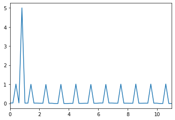
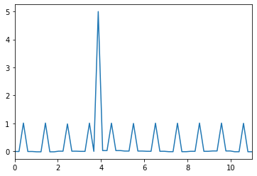
(a) The functions $f_{0}$, $f_{3}$ belonging to the simulated data set decribed in Section B.2.

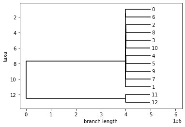
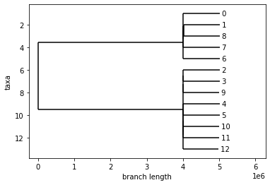
(b) The merge trees $(T_{f_{0}},h_{f_{0}})$ and $(T_{f_{3}},h_{f_{3}})$ associated to the functions in Figure 8(a).

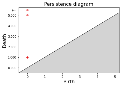
(c) The persistence diagram representing the functions in Figure 8(a). The point $(0,1)$ has multiplicity equal to the number of local minima minus $1$.

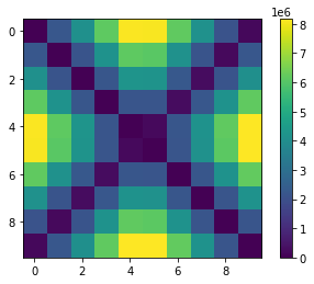
(d) Matrix of pairwise distances of the merge trees obtained from $\{f_{i}\}_{i=0}^{10}$.

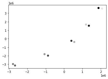
(e) Multidimensional Scaling Embedding in $\mathbb{R}^{2}$ of the matrix of pairwise distances shown in Figure 8(d). The shades of gray describe, from white to black, the ordering of the trees.

Figure 8: Plots related to the simulated scenario presented in Section B.2.

B.3 Edit Distance Between Merge Trees (Sridharamurthy et al., 2020) and Wasserstein Distance (Pont et al., 2022)

The edit distance in Sridharamurthy et al. (2020) is similar to classical edit distances, with the edit operations being restricted to insertion and deletion of vertices and with a relabeling operation which is equivalent to our shrinking operation. There is however the caveat that vertices are in fact understood as persistence pairs $(m,s)$, with $m$ being the leaf representing the local minimum giving birth to the component and $s$ the internal vertex representing the saddle point where the components merge with an earlier born component and thus dies according to the elder rule. There is thus a one-to-one correspondence between persistence pairs in the merge tree and in the associated persistence diagram. Editing a vertex $m$ implies editing also its saddle point $s$: deleting $(m,s)$ means deleting all vertices $m^{\prime}$ such that their persistent pair $(m^{\prime},s^{\prime})$ satisfies $s^{\prime}<s$. If then $s$ becomes of order $2$, it is removed. In particular the authors highlight the impossibility to make any deletion - with the word “deletion” to be understood according to our notation - on internal vertices, without deleting a portion of the subtree of the vertex. So they cannot delete and then insert edges to swap father-children relationships. To mitigate the effects of such issue, as a preprocessing step, they remove in a bottom-up fashion all saddles $s\in V_{T}$ such that $w_{T}((s,s^{\prime}))<\varepsilon$ for a certain positive threshold $\varepsilon$. All persistent pairs of the form $(m,s)$ are turned into $(m,s^{\prime})$. Such issue is further discussed in Section B.6.

Two merge trees are then matched via mappings representing these edit operations. To speed up the computations, the set of mappings between the trees is constrained so that disjoint subtrees are matched with disjoint subtrees. The cost of the edit operation on an edit pair $(m,s)$ is equal to the edit operation being applied on the corresponding points in the associated persistence diagrams with the $1$-Wasserstein distance: deleting a persistent pair has the cost of matching the corresponding point to the diagonal and relabeling a persistent pair with another in the second tree has the cost of matching the two points of the two diagrams - see (Sridharamurthy et al., 2020) Section 4.3.1.

A closely related metric between merge trees is the Wasserstein distance defined in Pont et al. (2022), which extends the metric by Sridharamurthy et al. (2020) producing also further analysis on the resulting metric space of merge trees by addressing the problem of barycenters and geodesics. In this work the authors rely on a particular branch decomposition of a merge tree, as defined in Wetzels et al. (2022), from which they induce the branch decomposition tree (BDT - Pont et al. (2022), Section 2.3) used to encode the hierarchical relationships between persistence pairs. A branch decomposition is roughly a partition of the graph $T$ of a merge tree $(T,h_{T})$ via ordered sequences of adjacent vertices (Wetzels et al., 2022). The chosen branch decomposition is the one induced by the elder rule and persistence pairs. Edit operations on such BDTs entail improved matchings and deletions between persistence pairs. To obtain the (squared) $2$-Wasserstein distance the vertices of two BDTs are match and the resulting costs are squared and then added. However, the authors then explain that with this first definition geodesics cannot by found via linear interpolation of persistence pairs for the hierarchical structure of the merge tree can be broken. To mitigate that, they employ a normalization which shrinks all the branches on $[0,1]$, irrespective of their original persistence - Pont et al. (2022), Section 4.2 - leading to simple geodesics obtained with linear interpolation between persistence pairs. To mitigate for this invasive procedure they introduce yet another preprocessing step artificially modifying small persistence features to reduce the normalization effects.

Some of the limitations of this approaches are listed in Pont et al. (2022), Section 7.3. Wetzels et al. (2022), Section 3.3 adds on that with further details and examples. Namely, the restricted space of possible matchings between trees - which is key to obtain the computational performances of the metrics - forces unstable behaviours: issues with saddle swaps (see Pont et al. (2022), Section 4.4 and Fig. 10) and instability of persistence pairs, so that elder ruled-based matchings may force very high persistence features to be matched with other very high persistence features even in situations where this implies making many unreasonable changes in the tree structures as in Figure 10(f) (see also Wetzels et al. (2022), Figure 1, Figure 2 b), Section 3.3, and Pont et al. (2022), Section 7.3). Moreover, Pont et al. (2022) does not address the interactions between the normalization and the two preprocessing steps..

B.4 Branch Decomposition-Independent Edit Distances for Merge Trees (Wetzels et al., 2022)

The work Wetzels et al. (2022) starts from the shortcomings of Sridharamurthy et al. (2020) and Pont et al. (2022) trying to overcome them. Namely it defines branch decompositions, - for instance, the perstence pairs of Sridharamurthy et al. (2020), induce one such branch decomposition - and in order to avoid issues related with the instability of the persistence pairs, Wetzels et al. (2022) introduce also the possibility to optimize the chosen branch decomposition. The only big issue with such approach is that it does not define a metric on the space of merge trees, for the triangle inequality is not satisfied - see Wetzels et al. (2022) Theorem 2 and Figure 3.

B.5 Heights vs Weights

In this section we try to better understand the different behaviour of $d_{E}$ when compared to the persistence-based metrics presented in the previous sections. The basic idea is that $w_{T}$ encodes the reciprocal positions of the merging points, instead of having the persistence pairs being free to move independently - at least locally - inside a constrained space.

(a) Two merge trees $T$ (left) and $T^{\prime}$ (right). We first delete $(e^{\prime},f^{\prime})$ and then edit $T$ with the shrinking defined by $(v,v^{\prime})$.

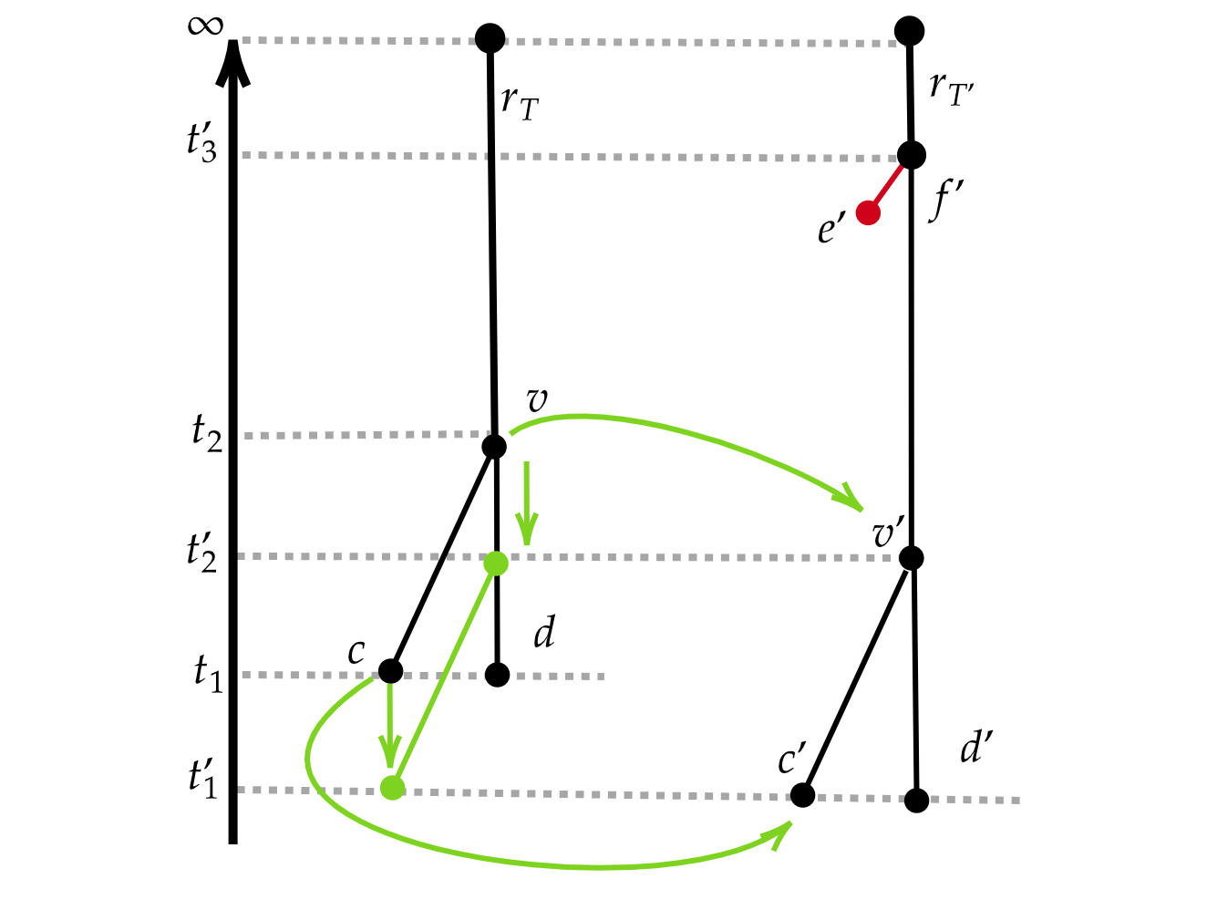
(b) The same merge trees as in Figure 9(a) - with some edges drawn at different angles for visualization purposes. We edit $T$ matching the persistence pair $(c,v)$ with $(c^{\prime},v^{\prime})$ according to Sridharamurthy et al. (2020); Pont et al. (2022).

(c) The results of the edits applied on $T$ in Figure 9(a) (left) and in Figure 9(a) (right)

.

Figure 9: A comparison between the weight based edits on which is based $d_{E}$, and the persistence based edits in Sridharamurthy et al. (2020); Pont et al. (2022).

Consider for instance the merge trees in Figure 4(b): the persistence pairs are $(c,v)$ and $(d,r_{T})$. The pairs of the rightmost tree instead are $(c^{\prime},v^{\prime}),(e^{\prime},f^{\prime})$ and $(d^{\prime},r_{T^{\prime}})$. Deleting $(e^{\prime},f^{\prime})$ according to Sridharamurthy et al. (2020); Wetzels et al. (2022); Pont et al. (2022) amounts to deleting $e^{\prime}$ according to our framework. Instead, shrinking $(v,r_{T})$ on $(v^{\prime},r_{T^{\prime}})$, after the deletion of $(e^{\prime},f^{\prime})$, for us means lengthening $(v,r_{T})$ by $t_{2}-t^{\prime}_{2}$ and so lowering $v$ and all the vertices below $v$ by the same amount, as in Figure 9(a). On the other hand, matching the persistence pair $(c,v)$ with $(c^{\prime},v^{\prime})$ for Sridharamurthy et al. (2020); Pont et al. (2022) is equivalent to shifting the edge $(c,v)$ downwards towards $(c^{\prime},v^{\prime})$ leaving all other vertices fixed, as in Figure 9(b). We can compare the results of such edits in Figure 9(c).

Thus, given a persistence pair $(m,s)$ inside a merge tree, corresponding to the point $(b,d)$ inside the persistence diagram, moving $s$ upwards by some $\varepsilon>0$ such that $h_{T}(s)+\varepsilon<h_{T}(s^{\prime})$ costs $\varepsilon$ in terms of the other edit distances, of the interleaving distance and in terms of the $1$-Wasserstein distance between persistence diagrams and leaves all other points with the same height. In terms of the edit distance $d_{E}$, instead, moving $s$ upwards by $\varepsilon>0$ shortens the edge above $s$ keeping all other edges of a fixed lengths and thus moves the vertices upwards by $\varepsilon$.

We can interpret this fact as the metrics in Morozov et al. (2013), Sridharamurthy et al. (2020) and Pont et al. (2022) better capturing similarities between trees via the location of their vertices in terms of heights; while $d_{E}$ better captures the “shape” of the tree i.e. relative positions of its vertices, being less sensible on the height variability since you can move more vertices at one. And this is exactly what happens in the example $f:I\rightarrow\mathbb{R}$ and $g(x)=f(x)+h$ - as in Figure 9: we have $d_{W_{1}}(PD(T),PD(G))=d_{E}(T,T^{\prime})(\dim(T)+\dim(G))$.

B.6 Stability vs Preprocessing

As already mentioned, the metrics in Sridharamurthy et al. (2020) and Pont et al. (2022) lack stability properties which means that there are certain situations in which such metrics measure variability between the trees which is undesirable as they may perceive as very far trees which are in fact very close in terms of interleaving distance. In particular they are unable to model “saddle swaps”, that is, with our terminology, deleting and inserting internal vertices to change father-children relationships. As noted also by the authors themselves, this issue needs to be addressed in some way. To do so authors resort to a computational solution implemented as a preprocessing step: they fix a threshold $\varepsilon>0$ for any couple of persistence pairs $(m,s)$ and $(m^{\prime},s^{\prime})$ with $s^{\prime}>s$ and $s^{\prime}-s<\varepsilon$, they change $(m,s)$ into $(m,s^{\prime})$ merging the two saddle points - in a bottom-up recursive fashion.

In this section, we produce a brief investigation of such procedure, which is absent in the aforementioned works. We represent the possible outcomes of this preprocessing in Figure 10. All merge trees in Figure 10 are drawn with colors representing persistence pairs, and similar colors yields persistence pairs with the same persistence throughout the whole figure. They ideally should be matched by the metrics to achieve optimal distances as the differences between edges of different colors could be arbitrary big.

In Figure 10(a) (left) we suppose that the edges marked with a red cross represent distances between saddles smaller or equal than $\varepsilon>0$, thus we recursively merge each saddle point with the higher one, starting from the bottom and going upwards. In this way we obtain the merge tree $T^{\prime}$ in Figure 10(a) (right) which is then used as input for the metric.

In Figure 10(b) we see two merge trees $T$ and $G$ such that their interleaving distance is $\varepsilon+\varepsilon^{\prime}$, for we need to move points of $T$ upwards by $\varepsilon+\varepsilon^{\prime}$ to match persistence pairs of the same color in $G$. Their edit distance $d_{E}$ would be $3(\varepsilon+\varepsilon^{\prime})$ for we need to delete and then insert back three small edges in $T$ to swap father-children relationships in a suitable way. Note that one can replicate analogous situations to make the interleaving distance between the two merge trees high at will: informally speaking it is enough to add other persistence pairs as needed and force matchings between pairs in very “different positions”.

In Figure 10(c) we see a possible output of the preprocessing routine. If the preprocessing threshold is bigger than $\varepsilon$ and $\varepsilon^{\prime}$ then the pre-processed trees $T^{\prime}$ and $G^{\prime}$ are equal. This in some sense is the desired output of the authors of Sridharamurthy et al. (2020) and Pont et al. (2022) for now their metric can match the colors of the persistence pairs. They suggest that such loss of variability - $d(T^{\prime},G^{\prime})=0$ even if $T\ncong_{2}G$ - could be mitigated by adding to the distance between the preprocessed trees the fixed threshold as many times as there are saddles merging in the procedure. Note that, if this artificial addition approximately matches the variability removed from the pairs attached to the orange vertical pair, it introduces artificial variability at the level of the branches attached to the brown edge, for they do not need any modification to be matched correctly.

In Figure 10(d), instead, we suppose that the preprocessing threshold is smaller than $\varepsilon$ and $\varepsilon^{\prime}$. The metrics then are forced to match persistence pairs with different colors causing an excess of variability which is pictured with red edges in the figure. We point out that, depending on the weights of the persistence pairs involved, these edges could be of arbitrary length.

In Figure 10(e) we represent the last possible output of the preprocessing procedure, which is a situation in which the threshold we fix is greater that $\varepsilon^{\prime}$ but smaller then $\varepsilon$. This is possibly the worst scenario: pairs are matched in an optimal way but we have introduced a lot of artificial variability, symbolized with red edges, in $G$. Again, because of additive phenomena caused by recursive saddle merging, these edges can be arbitrarily long.

Note that the preprocessing does not fix the issues presented in Figure 10(f), in Wetzels et al. (2022), Figure 1, Figure 2 b), Section 3.3, and Pont et al. (2022), Section 7.3.

(a) A merge tree $T$ (left) with its pre-processed version (right) according to the procedure in Sridharamurthy et al. (2020); Pont et al. (2022).

(b) Two merge trees $T$ and $G$ which are going to be preprocessed as in Section B.6.

(c) A possible output of the preprocessing: the preprocessing threshold is bigger than $\varepsilon$ and $\varepsilon^{\prime}$.

(d) Another possible output of the preprocessing: the preprocessing threshold is smaller than $\varepsilon$ and $\varepsilon^{\prime}$.

(e) The last possible output of the preprocessing: the preprocessing threshold is smaller than $\varepsilon$ and but bigger than $\varepsilon^{\prime}$.

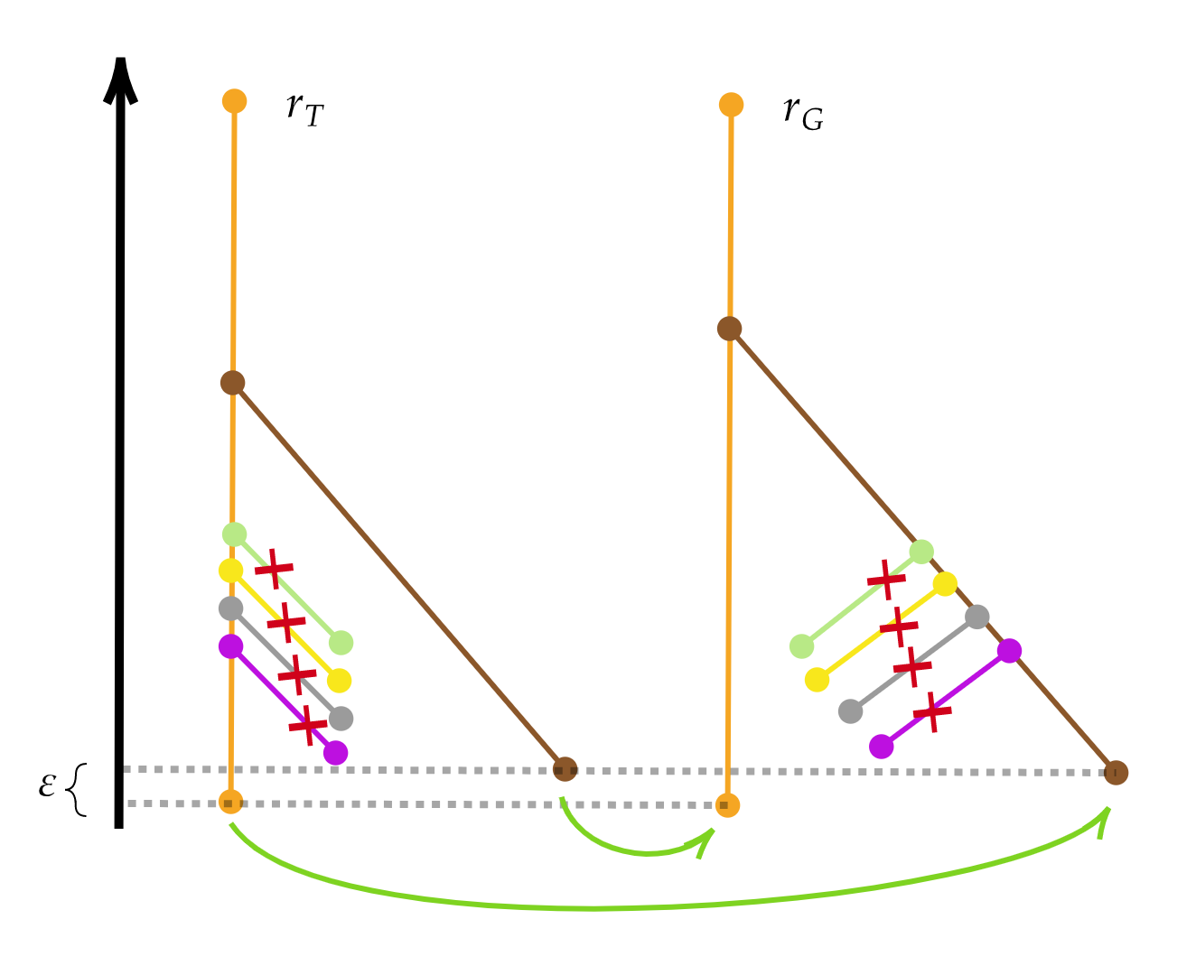
(f) As noted by Wetzels et al. (2022) and Pont et al. (2022), metrics which are based on persistence pairs may force unnatural scenarios like deleting all the pairs with the red cross, in order to match the orange and the brown persistence pairs of $T$, respectively, with the orange and the brown of $G$. Instead, it would be much more natural to match the orange and the brown ones according to the green arrows and then matching the other pairs according to colors.

Figure 10: Plots related to Section B.6

To conclude, we point out the following fact. We deem fundamental to have metrics being able to measure different kinds of variability in a data set, especially if the information captured is interpretable, however, any attempt to adapt our edit distance $d_{E}$ to work with heights instead of weights, would face the problem of coherently define deletion edits. While it seems reasonable to have $w_{T}((v,v^{\prime}))$ as a cost to delete and edge - for instance, this cost amounts to the persistence of the feature if $(v,v^{\prime})$ is a persistence pair - any change in the height of $v^{\prime}$ changes the weight of $(v,v^{\prime})$ and thus the cost of its deletion, invalidating all the results about mappings in Pegoraro (2021b) and the algorithm therein. Similarly, adapting Sridharamurthy et al. (2020) or Pont et al. (2022) to handle saddle swaps, would mean at least removing from their mappings, the property that would be (M3) in our notation, creating many issues from the theoretical and computational point of view. In fact, internal edges are not really available in the representation used by such metrics, where all points are instead understood as part of a persistence pair.

C Proofs

Proof of 1.

Consider $(T,h_{T})$ and $(T^{\prime},h_{T^{\prime}})$ such that $\max h_{T}<K^{\prime}$ and $\max h_{T^{\prime}}<K^{\prime}$. Consider $(G,w_{G})=\mathcal{T}_{K^{\prime}}((T,h_{T}))$ and $(G^{\prime},w_{G^{\prime}})=\mathcal{T}_{K^{\prime}}((T^{\prime},h_{T}))$. For any $K$ such that $\max h_{T}<K<K^{\prime}$ and $\max h_{T^{\prime}}<K<K^{\prime}$ there is a splitting of $(v,r_{G})\in E_{G}$ with a vertex $w$ and a splitting of $(v^{\prime},r_{G^{\prime}})$ with a vertex $w^{\prime}$ such that the obtained weighted trees $(R,w_{R})$ and $(R^{\prime},w_{R^{\prime}})$ satisfy: $w_{R}((w,r_{G}))=w_{R^{\prime}}((w^{\prime},r_{G^{\prime}}))$. Thus by 4 we obtain $d_{E}(G,G^{\prime})=d_{E}(R,R^{\prime})=d_{E}(sub_{R}(w),sub_{R^{\prime}}(w^{\prime}))$. Moreover, $sub_{R}(w)=\operatorname*{Tr}_{K}((T,h_{T}))$ and $sub_{R^{\prime}}(w^{\prime})=\operatorname*{Tr}_{K}((T^{\prime},h_{T^{\prime}}))$.

Being $K,K^{\prime}$ arbitrary we have that $d_{K}((T,h_{T}),(T^{\prime},h_{T^{\prime}}))$ does not depend on $K$, for $K>\max\{\max h_{T},\max h_{T^{\prime}}\}$. We need to prove the case $K=\max\{\max h_{T},\max h_{T^{\prime}}\}$.

Let $(G,w_{G})=\mathcal{T}_{K}((T,h_{T}))$ and $(G^{\prime},w_{G^{\prime}})=\mathcal{T}_{K^{\prime}}((T,h_{T}))$, for $K^{\prime}>K$. And consider now the weighted tree $\star=(\{\star\},w(\emptyset)=0)$,

We have that $d_{E}(G,\star)=\sum_{e\in E_{G}}w_{G}(e)$ and $d_{E}(G^{\prime},\star)=\sum_{e\in E_{G^{\prime}}}w_{G^{\prime}}(e)$. Thus by the reversed triangle inequality - 8:

$$\mid d_{E}(G,\star)-d_{E}(G^{\prime},\star)\mid=K^{\prime}-K\leq d_{E}(G,G^{\prime}),$$

So we have:

$$d_{E}(\mathcal{T}_{K^{\prime}}((T,h_{T})),\mathcal{T}_{K}((T,h_{T})))=K^{\prime}-K.$$

and we can set $K=\max\{\max h_{T},\max h_{T^{\prime}}\}$ and take $K^{\prime}\rightarrow K$ to finish the proof.

$\blacksquare$

Proof of 5.

Let $\pi_{0}(X_{\operatorname*{\scalerel*{\cdot}{\bigodot}}})$ and $\pi_{0}(Y_{\operatorname*{\scalerel*{\cdot}{\bigodot}}})$ be two regular abstract merge trees which are represented by the merge trees $(T,h_{T})$ and $(G,h_{G})$, which we represent as weighted trees via the some $\operatorname*{Tr}_{K}$. The proof is quite long and requires some technical definitions. We split it into different parts to make it more easily readable.

Introduction - Display Posets

For ease of notation, we introduce the following objects.

Definition 27 (Curry et al. (2022))

Given a persistent set $S:\mathbb{R}\rightarrow\operatorname*{Sets}$ we define its display poset as:

$$D_{S}:=\bigcup_{t\in\mathbb{R}}S(t)\times\{t\}.$$

The set $D_{S}$ can be given a partial order with $(a,t)\leq(b,t)$ if $S(t\leq t^{\prime})(a)=b$.

Let $D_{\pi_{0}(X_{\operatorname*{\scalerel*{\cdot}{\bigodot}}})}$ and $D_{\pi_{0}(Y_{\operatorname*{\scalerel*{\cdot}{\bigodot}}})}$ be the display posets induced by $\pi_{0}(X_{\operatorname*{\scalerel*{\cdot}{\bigodot}}})$ and $\pi_{0}(Y_{\operatorname*{\scalerel*{\cdot}{\bigodot}}})$. We call $h_{\pi_{0}(X_{\operatorname*{\scalerel*{\cdot}{\bigodot}}})}$ the height function of $D_{\pi_{0}(X_{\operatorname*{\scalerel*{\cdot}{\bigodot}}})}$ and $h_{\pi_{0}(Y_{\operatorname*{\scalerel*{\cdot}{\bigodot}}})}$ the height function of $D_{\pi_{0}(Y_{\operatorname*{\scalerel*{\cdot}{\bigodot}}})}$.

Introduction - Couplings

The content of this part of the proof is taken from Pegoraro (2021a).

We leverage on the notion of couplings between merge trees defined in Pegoraro (2021a). Before recalling such definition that we highlight a subtle difference in merge trees as defined in Pegoraro (2021a) wrt respect to the definition we give here. In Pegoraro (2021a) the edge going to infinity which we require in our merge trees - $(v,r_{T})$ with $h_{T}(r_{T})=\infty$ - is not needed and thus such edge is removed. In other words, a merge tree $(T,h_{T})$ is the sense of Pegoraro (2021a) is such that $ord_{T}(r_{T})>1$ and $h_{T}(r_{T})\in\mathbb{R}$. we state the results in Pegoraro (2021a) with the notation of the present manuscript.

Consider $C\subset V_{T}\times V_{G}$ and the projection $\pi_{T}:V_{T}\times V_{G}\rightarrow V_{T}$, we define the multivalued map $\Lambda_{C}^{T}:V_{T}\rightarrow V_{T}$ as follows:

$$\Lambda_{C}^{T}(v)=\begin{cases}\max_{v^{\prime}<v}\pi_{T}(C)&\text{if }\#\{v^{\prime}\in V_{T}\mid v^{\prime}<v\text{ and }v^{\prime}\in\pi_{T}(C)\}>0\\ \emptyset&\text{otherwise.}\end{cases}$$

The term “multivalued” means that $\Lambda_{C}^{T}$ is a function $\Lambda_{C}^{T}:V_{T}\rightarrow\mathcal{P}(V_{T})$ with $\mathcal{P}(V_{T})$ being the power set of $V_{T}$.

A coupling between the merge trees $(T,h_{T})$ and $(G,h_{G})$ - with the definition given in the present work - is then a set $C\subset V_{T}-\{r_{T}\}\times V_{G}-\{r_{G}\}$ such that:

• $\#\max C=1$ or, equivalently, $\#\max\pi_{T}(C)=\#\max\pi_{G}(C)=1$

• the projection $\pi_{T}:C\rightarrow V_{T}$ is injective (the same for $G$)

• given $(a,b)$ and $(c,d)$ in $C$, then $a<c$ if and only if $b<d$

• $a\in\pi_{T}(C)$ implies $\#\Lambda_{C}^{T}(a)\neq 1$ (the same for $G$).

Similarly to mappings each couple in $C$ is associated to a cost, and $\parallel C\parallel_{\infty}$ is defined as the highest of such costs. In Pegoraro (2021a) it is proven that $d_{I}(T,G)\leq\parallel C\parallel_{\infty}$ for all couplings $C$.

Define the following functions as in Pegoraro (2021a):

• define $\varphi_{C}^{T}:V_{T}\rightarrow V_{T}$ so that $\varphi_{C}^{T}(x)=\min\{v\in V_{T}\mid v>x\text{ and }\#\Lambda(v)\neq 0\}$. Note that since the set $\{v\in V_{T}|v>x\}$ is totally ordered, $\varphi_{C}^{T}(x)$ is well defined;

• similarly, define $\delta_{C}^{T}:V_{T}\rightarrow V_{T}$, defined as $\delta_{T}(x)=\min\{v\in V_{T}\big{|}v\geq x\text{ and }v\in\pi_{T}(C)\}$;

• set $\gamma^{C}_{T}:V_{T}-D_{C}^{T}\rightarrow V_{G}$ to be:

  $$\gamma^{C}_{T}(x)=\begin{cases}\arg\min\{g(w)\mid(v,w)\in C,v<x\}&\text{if }\#\{g(w)\mid(v,w)\in C,v<x\}>0\\ \emptyset&\text{otherwise.}\end{cases}$$

  Note that if $\#\{g(w)\mid(v,w)\in C,v<x\}>0$, by (G), $\gamma^{C}_{T}(x)$ is uniquely defined. Moreover, $\gamma^{C}_{T}(\varphi^{C}_{T}(x))$ is well defined for any $v\in V_{T}$;

• lastly, set $\eta_{C}^{T}(x):=\gamma_{C}^{T}(\varphi_{C}^{T}(x))$.

To lighten the notation, when clear from the context, we may omit subscripts and superscripts. The costs of a coupling are defined in Pegoraro (2021a) as follows.

• if $(x,y)\in C$, $cost_{C}(x)=|h_{T}(x)-h_{G}(y)|$;

• if $x\notin\in\pi_{T}(C)$, we have two different scenarios:

  • if $\#\Lambda(x)=0$, then $cost_{C}(x)=\max\{\left(h_{T}(\varphi(x))-h_{T}(x)\right)/2,h_{G}(\eta(x))-f(x)\}$;

  • if $\#\Lambda(x)>1$, we have $cost_{C}(x)=\mid h_{T}(x)-h_{G}(w)\mid$ with $(\delta(x),w)\in C$;

  • zero otherwise.

Lastly, in Pegoraro (2021a) it is shown that, via $C$ one can induce

$$\alpha_{C}:D_{\pi_{0}(X_{\operatorname*{\scalerel*{\cdot}{\bigodot}}})}\rightarrow D_{\pi_{0}(Y_{\operatorname*{\scalerel*{\cdot}{\bigodot}}})}\text{ and }\beta_{C}:D_{\pi_{0}(Y_{\operatorname*{\scalerel*{\cdot}{\bigodot}}})}\rightarrow D_{\pi_{0}(X_{\operatorname*{\scalerel*{\cdot}{\bigodot}}})}$$

such that

$$cost_{C}(v)=\mid h_{\pi_{0}(Y_{\operatorname*{\scalerel*{\cdot}{\bigodot}}})}(\alpha_{C}(v))-h_{\pi_{0}(X_{\operatorname*{\scalerel*{\cdot}{\bigodot}}})}(v)\mid$$

for any $v\in V_{T}$ and

$$cost_{C}(w)=\mid h_{\pi_{0}(X_{\operatorname*{\scalerel*{\cdot}{\bigodot}}})}(\beta_{C}(w))-h_{\pi_{0}(Y_{\operatorname*{\scalerel*{\cdot}{\bigodot}}})}(w)\mid$$

for any $w\in V_{G}$.

Main body of the proof

We now want to establish relations between mappings between $\operatorname*{Tr}_{K}((T,h_{T}))$ and $\operatorname*{Tr}_{K}((G,h_{G}))$ - with $K>\max h_{T},\max h_{G}$ - and couplings between $(T,h_{T})$ and $(G,h_{G})$. When working with $\operatorname*{Tr}_{K}((T,h_{T}))$ and $\operatorname*{Tr}_{K}((G,h_{G}))$ we can apply the following result from Pegoraro (2021b).

Corollary 9 (Pegoraro (2021b))

Given $(T,w_{T})$ and $(T^{\prime},w_{T^{\prime}})$ weighted trees. If $r_{T}$ and $r_{T^{\prime}}$ are of order $1$, for any minimizing mappings $M$, then neither $(v,r_{T})$ or $(w,r_{T^{\prime}})$ are deleted and we have $\#\max M=1$.

Given a minimizing mapping $M\in M_{2}(T,T^{\prime})$, thanks to 1, we have that $a\in\pi_{T}(M)$ implies $\#\Lambda_{M}^{T}(a)\neq 1$ (the same for $G$). In fact (C4) is equivalent to having no vertices of order two after deletions and ghostings. This means that $C_{M}:=C(M)=\{(a,b)\in M\mid a\in V_{T}\text{ and }b\in V_{G}\}$ is a coupling.

Conversely, given a minimizing coupling $C$, the set

$$M_{C}:=C \bigcup\{(a,"D")\mid a\notin\pi_{T}(C)\text{ and }\#\Lambda_{C}^{T}(a)\neq 1\}$$

$$\bigcup\{("D",b)\mid b\notin\pi_{G}(C)\text{ and }\#\Lambda_{C}^{G}(b)\neq 1\}$$

$$\bigcup\{(a,"G")\mid a\notin\pi_{T}(C)\text{ and }\#\Lambda_{C}^{T}(a)=1\}$$

$$\bigcup\{("G",b)\mid b\notin\pi_{G}(C)\text{ and }\#\Lambda_{C}^{G}(b)=1\}$$

is a mapping. Clearly $M_{C_{M}}=M$ and $C_{M_{C}}=C$.

Now we prove the following lemma.

Lemma 3

Let $f:[a,K]\rightarrow[b,K]$ be a monotone function such that $f(K)=K$, $K\in\mathbb{R}$. For every $\{x_{1}<\ldots<x_{n+1}=K\}\subset[a,K]$:

$$\max_{i=1,\ldots,n+1}d(f(x_{i}),x_{i})\leq\sum_{i=1}^{n}\mid d(x_{i},x_{i+1})-d(f(x_{i}),f(x_{i+1}))\mid$$ (3)

Proof  Let $v_{i}=f(x_{i})-x_{i}$. And let $m\in\{1,\ldots,n+1\}$ be such that $\mid f(x_{m})-x_{m}\mid=\max\mid f(x_{i})-x_{i}\mid$.

Then we set:

$$v_{1}= v_{m}+\varepsilon_{1}$$

$$v_{2}= v_{m}+\varepsilon_{1}+\varepsilon_{2}$$

$$\ldots$$

$$v_{i}= v_{m}+\sum_{j=1}^{i}\varepsilon_{j}$$

$$\ldots$$

$$v_{n}= v_{m}+\sum_{j=1}^{n}\varepsilon_{j}.$$

Thus we can write Equation 3, which we need to prove, as:

$$\mid v_{m}\mid\leq\sum_{i}\mid x_{i}-f(x_{i})-(x_{i+1}-f(x_{i+1}))\mid=\sum_{i}\mid v_{i}-v_{i+1}\mid=\sum_{i=1}^{n}\mid\varepsilon_{i+1}\mid.$$

Clearly we have some constraints on $\varepsilon_{i}$, in fact:

$$x_{i}+v_{m}+\sum_{j=1}^{i}\varepsilon_{j}\leq x_{i+1}+v_{m}+\sum_{j=1}^{i+1}\varepsilon_{j}$$

which means:

$$x_{i}-x_{i+1}\leq\varepsilon_{i+1}.$$

In particular $x_{n}+v_{n}=x_{n}=1$ means that $v_{m}+\sum_{j=1}^{n}\varepsilon_{j}=0$ i.e. $-v_{m}=\sum_{j=1}^{n}\varepsilon_{j}$. Thus:

$$\mid v_{m}\mid=\mid\sum_{j=1}^{n}\varepsilon_{j}\mid\leq\sum_{i=1}^{n}\mid\varepsilon_{i+1}\mid.$$

 

Consider now a leaf $l\in L_{T}$ and take $\zeta_{l}=\{p\in V_{T}\mid v\geq l\}$. Consider the interval $[h_{T}(l),K]$. The map $v\in\zeta_{l}\mapsto h_{T}(v)$ gives a $1:1$ correspondence between $\zeta_{l}$ and a finite collection of points in $[h_{T}(l),K]$. We define $f(h_{T}(v))=h_{\pi_{0}(Y_{\operatorname*{\scalerel*{\cdot}{\bigodot}}})}(\alpha_{C}(v))$ for $v\in\zeta_{l}-\{r_{T}\}$. And $f(K)=K$. Note that $\alpha_{C}$ is constructed such that $\alpha_{C}(v)=w$ if $(v,w)\in C$. Thus $f(h_{T}(v))\leq K$ for $v\in\zeta_{l}$.

We extend $f$ on $[h_{T}(l),K]$ via linear interpolation. Since $\alpha_{C}$ is monotone wrt the partial order on $D_{\pi_{0}(X_{\operatorname*{\scalerel*{\cdot}{\bigodot}}})}$, then $f$ is monotone on $[h_{T}(l),K]$.

Now consider $T$ and apply on it all the deletions and ghostings which involve points which are not in $\zeta_{l}$. We call $\{v_{1}=l<\ldots<v_{n+1}=r_{T}\}$ the coupled points in $\zeta_{l}$. Then:

$$\mid h_{T}(v_{i})-h_{T}(v_{i+1})-f(h_{T}(v_{i}))-f(h_{T}(v_{i+1}))\mid\leq cost_{M_{C}}([v_{i},v_{i+1}]\mapsto[\alpha_{C}(v_{i}),\alpha_{C}(v_{i+1})])$$ (4)

With $cost_{M_{C}}([v_{i},v_{i+1}]\mapsto[\alpha_{C}(v_{i}),\alpha_{C}(v_{i+1})])$ being the cost of the edits associated to points $v_{i}\leq p\leq v_{i+1}$ and $\alpha_{C}(v_{i})\leq q\leq\alpha_{C}(v_{i+1})$. In fact we have equality in Equation 4 if there are no deletions for any $p\in V_{T}$ such that $v_{i}\leq p\leq v_{i+1}$ and any $q\in V_{T^{\prime}}$ such that $\alpha_{C}(v_{i})\leq q\leq\alpha_{C}(v_{i+1})$. Otherwise the total cost of the deletions and shrinking exceeds $\mid h_{T}(v_{i})-h_{T}(v_{i+1})-f(h_{T}(v_{i}))-f(h_{T}(v_{i+1}))\mid$ since:

$$\mid n_{1}+n_{2}-(n_{3}+n_{4})\mid\leq n_{1}+n_{3}+\mid n_{2}-n_{4}\mid$$

with $n_{i}\in\mathbb{R}_{\geq 0}$. Lastly note that $\mid h_{T}(v_{i})-f(h_{T}(v_{i}))\mid=cost_{C}(v)$.

By 3, we have:

$$\max cost_{C}(v_{i})= \max h_{T}(v_{i})-f(h_{T}(v_{i}))$$ (5)

$$\leq \sum_{i=1}^{n}\mid h_{T}(v_{i})-f(h_{T}(v_{i}))+f(h_{T}(v_{i+1})-h_{T}(v_{i+1})\mid$$

$$\leq cost_{M_{C}}([l,r_{T}]\mapsto[w,r_{G}])$$

with $(v,w)\in M_{C}$ and $v=\min\zeta_{l}\cap\pi_{T}(C)$.

Conclusion

Let $\parallel C\parallel_{\infty}=cost_{C}(x)$. WLOG $x\in V_{T}$. Then $x\in\zeta_{l}$ for some $l\in L_{T}$. By applying Equation 5 we obtain the result.

$\blacksquare$

Proof of 3.

By Section 6.1 we can consider only weighted trees such that $T_{2}=T$.

1. Given $\lambda\in[0,1]$ and $T\in\mathcal{T}$ we define $\lambda\cdot T$ to be the tree obtained by shrinking each edge of $T$ by a factor of $\lambda$ i.e. if $w^{\prime}$ is the weight function of $\lambda\cdot T$, we have $w^{\prime}(v)=\lambda\cdot w(v)$.

   Now consider $M\in\operatorname*{Mapp}(T,T^{\prime})$. We call $M_{\lambda}$ the same mapping but inside $\operatorname*{Mapp}(\lambda\cdot T,\lambda\cdot T^{\prime})$. Since we can take $\lambda$ outside the cost of all the edits, then $cost(M_{\lambda})=\lambda\cdot cost(M)$. In other words $d_{E}(\lambda\cdot T,\lambda\cdot T^{\prime})\leq\lambda\cdot d_{E}(T,T^{\prime})<d_{E}(T,T^{\prime})$.

   This of course implies that $F:[0,1]\times\mathcal{T}\rightarrow\mathcal{T}$, such that $F(t,T)=t\cdot T$ is continuous, and so $\mathcal{T}$ is contractible.

2. We prove that given for any tree $T$ and any $\varepsilon>0$, $B_{\varepsilon}(T)$ is not complete. Build the following Cauchy sequence: let $T_{0}=T$ and obtain the tree $T_{n}$ by attaching to a leaf of $T_{n-1}$ a pair of edges, each with length $\frac{\varepsilon}{2\cdot 2^{n}}$. Consider $n>m$, then $d_{E}(T_{n},T_{m})\leq\varepsilon\sum_{k=m}^{n}2^{-k}$ which is arbitrarily small as $n,m$ increase. Thus $\{T_{n}\}$ is a Cauchy sequence. Moreover $d_{E}(T,T_{n})\leq\varepsilon\sum_{k=0}^{n}2^{-k}\leq\varepsilon$ and thus $\{T_{n}\}\subset B_{\varepsilon}(T)$.

   Suppose that exists $T^{\prime}$ such that $T_{n}\rightarrow T^{\prime}$. By construction we know $\#V_{T_{n}}\rightarrow\infty$. Let $M_{n}\in\operatorname*{Mapp}(T_{n},T^{\prime})$ minimizing mapping. Clearly $cost(M_{n})\rightarrow 0$. For ease of notation we call $C_{n}:=C(M_{n})$ and $D_{n}:=(M_{n})_{D}$.

   By definition $\#C_{n}\leq K=\dim(T^{\prime})$. We know that all the vertices in $V_{T_{n}}-V_{T}$ have one sibling since they are added as couples. This means that, even if we take away $K$ vertices, at least one out of every pair of the remaining siblings will be deleted once $\dim(T_{n})>\dim(T^{\prime})$. Of course $cost(M_{n})\geq cost(C_{n})+cost(D_{n})$ and so $cost(D_{n})\rightarrow 0$.

   But $cost(D_{n})>\varepsilon\cdot\frac{1}{2}\sum^{n}_{K}\frac{1}{2^{n}}$ and so it does not go to zero.

   This shows that $C=\overline{B_{\varepsilon}(T)}$ is not compact. In fact $\{T_{n}\}\subset C$ is a Cauchy sequence but it is not converging.

3. We need to prove local compactness and we do so via sequential compactness.

   Consider $T\in\mathcal{T}^{N}$ and a sequence $\{T_{n}\}\subset\overline{B_{\varepsilon}(T)}$ with $\varepsilon<\min_{v\in V_{T}}w_{T}(v)$.

   If we consider an edge $l=(v,v^{\prime})$ in $T$, along the sequence $T_{n}$ we know that $l$ will never get wholly deleted. It might be split, shrunk but it will never disappear.

   We fix a sequence of mappings $M_{n}$ such that $M_{n}\in\operatorname*{Mapp}(T,T_{n})$ and $cost(M_{n})=d_{E}(T,T_{n})$. For any edge $l=(v,v^{\prime})$ in $T$, with $v<v^{\prime}$, we consider the set $E_{n}^{l}=\{e^{k}_{n}\}$ such that $e^{k}_{n}\in M_{n}$ edits the edge $l$. With that we mean: shrinkings of $l$, splittings which add points $w$ with $v<w<v^{\prime}$ (note that these appear only after the shrinkings), insertion of edges in points $w$ with $v\leq w\leq v^{\prime}$. Of course for each $n$, we might have $e^{1}_{n}$, $e^{2}_{n}$,… acting on the same edge. While there can be at most one shrinking on $l$ for each $n$, there can be multiple insertions or splittings; of course this number is uniformly bounded because of the dimension constraints.

   For a fixed $n$ we have a natural order between splittings, given by the height at which the new point is inserted, and a similarly induced partial ordering between insertions. Insertion are comparable with respect to this partial order if they happen at different heights. We fix a random order on insertions happening at the same vertex so that all insertions are completely ordered. For a fixed $l$ we partition these edits into $Sh^{n}$, $S^{n}_{k}$ and $I^{n}_{k^{\prime},k}$, which, for each $n$, collects the elements in $E_{n}^{l}$ which are respectively the shrinking, the $k$-th splitting and the $k$-th insertion at the $k^{\prime}$-th inserted vertex. One can set $k^{\prime}=0$ being the index of $v$, and $k^{\prime}=-1$ being the index of $v^{\prime}$.

   We know that for each edge $l$:

   • $Sh=\cup_{n}Sh^{n}$ is at most countable, and the sequence given by the different weights of $l$ obtained through the shrinkings, is a sequence in $[L-\varepsilon,L+\varepsilon]$, with $L$ the original length of $l$. Then we can extract a converging subsequence.

   • $S_{k}=\cup_{n}S^{n}_{k}$ is at most countable, then the ratio of the distance in height between $v$ and the splitting point, over the length of $l$ (after the shrinking of the $n$-th mapping) form a sequence in $[0,1]$. So we can extract a converging subsequence in $[0,1]$. In other words we can find a subsequence of edits which converges to a certain splitting.

   • $I_{k^{\prime},k}=\cup_{n}I^{n}_{k^{\prime},k}$ is at most countable for every $k,k^{\prime}$; the length of the inserted edges form a sequence in $[0,\varepsilon]$. So for every $k,k^{\prime}$ we can extract a converging subsequence.

   If some of the sets defined above are finite we discard from the sequence the indexes $n$ which appear in the collection of edit, being it $Sh$, $S_{k}$ or $I_{k,^{\prime}k}$. Note that, by the dimension bounds, we have a finite number of such sets, for a finite number of edges.

   Thus, for every edge $l$, we proceed in this way:

   1. since $Sh$ is countable we extract a converging subsequence of shrinkings.

   2. starting from $k=1$, from the subsequence just obtained we extract a converging subsequence of splitting locations. Starting from this sequence we repeat the extraction procedure for $k=2$, then recursively till we reach $k$ such that $S_{k}$ is empty. Again if, for some $k$, $S_{k}$ is finite, we simply discard elements of the subsequence appearing in $S_{k}$.

   3. lastly, from the last set of indexes we obtained, we extract from $I_{k^{\prime},k}$ a converging subsequence of insertions for every $k$ and $k^{\prime}$; working on $k$ and $k^{\prime}$ as in the previous point. In a finite number of steps we reach $I_{\widehat{k^{\prime}},\widehat{k}}$ such that for all $k^{\prime}>\widehat{k^{\prime}}$ and $k>\widehat{k}$, $I_{k,k^{\prime}}=\emptyset$.

   Given any ordering on the edges, we recursively apply this for every $l$, and obtain a subsequence which, with an abuse of notation, we still call $\{T_{n}\}$.

   We fix $n$ and take for every edge the edits in $Sh^{n}\cup_{k}S^{n}_{k}\cup_{k^{\prime},k}I^{n}_{k^{\prime},k}$. If we take the union of such edits over the edges $l$ we obtain a mapping $N_{n}$ for every $n$. The mapping $N_{n}$ is defined on $T$ and by construction is contained in $M_{n}$. Note that $N_{n}$ collects all the edits which are applied by $M_{n}$ on $T$ that is all the shrikings and splitting, plus all the insertions which are made directly on the vertices of $T$ or on the splittings already applied. In other words $M_{n}-N_{n}$ is made by insertions which are applied on edges which are obtained by other insertions.

   Call $ST_{n}$ the tree obtained from $T$ with the edits in $N_{n}$. Then clearly $N_{n}\in\operatorname*{Mapp}(T,ST_{n})$. For what we have said, $T_{n}$ can be obtained from $ST_{n}$ with the edits in $M_{n}-N_{n}$, which are only a particular case of insertions.

   By construction, any edit in $N_{n}$ is part of a converging sequence of edits: shrinking converge to a final weight value, splittings converge to a final position on the edge and insertions converge to a final weight of the inserted edge. We call $\overline{N}$ the mapping obtained with the limit of the edits of $N_{n}$. Clearly $cost(N_{n})\rightarrow cost(\overline{N})$. Let $ST$ be the tree obtained from $T$ with $\overline{N}$. We have $ST_{n}\rightarrow ST$. In fact, consider one edge $l\in E_{T}$. Take for instance the sequence of shrinkings in $Sh=\{e_{1},\ldots,e_{n},\ldots\}$ parametrized such that $w_{ST_{n}}(l)=e_{n}$ and $e_{n}\rightarrow e$. For any fixed $\epsilon>0$ and for $n$ big enough we know $|e_{n}-e|<\epsilon$. Thus $|w_{ST_{n}}(l)-w_{ST_{n+1}}(l)|<\epsilon$ is a shrinking with cost less then $\epsilon$. For the same edge $l$ there are at most $N$ splittings, each edit splits $l$ in $E_{ST_{n}}$ at a certain height. Similarly, the difference in heights between splittings in $S^{n}_{k}$ and $S^{m}_{k}$ with $m>n$ is going to zero, and thus we can again choose $n$ big enough so that the $k-$th splitting of $ST_{n}$ can be turned in the $k-$th splitting of $ST$, for all $k$, with cost less than $\epsilon$. The same reasoning can be done on the weights of the insertions. Thus we can go from $ST_{n}$ to $ST$ with a finite set of edits, with cost less that $\epsilon$ and whose number is uniformly bound. For instance we know that on every tree we can have at most $N$ shrinkings, $N$ ghostings, and $N$ insertions. Thus, for every $\epsilon$, there is $n$ big enough such that $d_{E}(ST_{n},ST)<3N\epsilon$. We remark that, since $N_{n}\subset M_{n}$, then $cost(N_{n})\leq\varepsilon$ for every $n$, and thus $d_{E}(T,ST)\leq\varepsilon$.

   At this point we have obtained a sequence $\{ST_{n}\}$ such that: $ST_{n}\rightarrow ST$ in $\overline{B_{\varepsilon}(T)}$ and $V_{ST_{n}}\subset V_{T_{n}}$. Then next natural step is to recursively “enlarge” $ST_{n}$.

   Take each $M_{n}$ and substitute each edit in $N_{n}\subset M_{n}$ with its limit $\overline{N}$, obtaining $\overline{M_{n}}$. Note that $cost(M_{n})\rightarrow cost(\overline{M_{n}})$ as $n$ grows.

   We can obtain a new sequence of trees $T^{\prime}_{n}$ and mappings $M^{\prime}_{n}\in\operatorname*{Mapp}(ST,T^{\prime}_{n})$ in this way:

   • $T^{\prime}_{n}$ is obtained from $T$ applying the mapping $\overline{M_{n}}$.

   • $M^{\prime}_{n}\in\operatorname*{Mapp}(ST,T^{\prime}_{N})$ is the mapping induced by the identifications given by the composition of the paths: $T\xrightarrow{\overline{N}}ST\xrightarrow{\overline{M_{n}}-\overline{N}}T^{\prime}_{n}$; which is well defined since $\overline{M_{n}}-\overline{N}$ is made only by insertions to be done on $ST$. Thus we can identify $M^{\prime}_{n}$ as given by the “identity” on the vertices of $ST$, and the edits in $M_{n}-N_{n}$, which, as already noted, are only insertions. We call $id_{ST}$ the set of couplings embedding $ST$ into $T^{\prime}_{n}$.

   The first thing we highlight is that, since $M_{n}\rightarrow\overline{M_{n}}$, in the sense that their edits converge as already explained, then $d_{E}(T_{n},T^{\prime}_{n})\rightarrow 0$. So in $\{T^{\prime}_{n}\}$ converges to a limit point, so does $\{T_{n}\}$. For the same reason we have that also $\{T^{\prime}_{n}\}$ is a Cauchy sequence.

   We can perform the steps which lead us to obtain $\{ST_{n}\}\rightarrow ST$ starting from $T$ and the sequence $\{T_{n}\}$, but taking $ST$ as “reference tree” and $\{T^{\prime}_{n}\}$ as initial sequence. So we obtain the subsequence of $\{ST_{n}\}$ which we use to build sequence $\{ST^{\prime}_{n}\}\rightarrow ST^{\prime}$ along with mappings $N^{\prime}_{n}\in\operatorname*{Mapp}(ST,ST^{\prime}_{n})$. For notational convenience, any time we throw away indexes from $\{T^{\prime}_{n}\}$, we remove the same indexes also from $\{T_{n}\}$.

   The key point is that $id_{ST}\subset N^{\prime}_{n}$ for all $n$ and, in particular, we have $ST\neq ST^{\prime}_{n}$ if and only if $id_{ST}\subsetneq N^{\prime}_{n}$. Since $M^{\prime}_{n}-N^{\prime}_{n}$ contains only insertions to be applied on edges which have already been inserted in $ST$, if there are no such edges, we have $ST=T^{\prime}_{n}$.

   Now we relate $\{ST^{\prime}_{n}\}\rightarrow ST^{\prime}$ with $T$ and $\{ST_{n}\}\rightarrow ST$. To do so, consider: $A_{n}=(N^{\prime}_{n}-id_{ST})\bigcup N_{n}$. By construction $A_{n}\in\operatorname*{Mapp}(T,ST^{\prime}_{n})$. For what we have said, either $N_{n}\subsetneq A_{n}$ or $ST=T^{\prime}_{n}$ and so $A_{n}=N_{n}=M_{n}$. On top of that $A_{n}\subset M_{n}$ and thus $d_{E}(T,ST^{\prime})\leq\varepsilon$. Now, call $SST_{n}$ the weighted tree obtained by editing $T$ with the edits contained in $A_{n}$: either $V_{ST_{n}}\subsetneq V_{SST_{n}}$ or $SST_{n}=T_{n}$. Moreover, since $N_{n}\rightarrow\overline{N}$ and $ST^{\prime}_{n}\rightarrow ST^{\prime}$ we get $SST_{n}\rightarrow ST^{\prime}$.

   Thus, this further step has produced a sequence of weighted trees $\{SST_{n}\}$ “bigger” than $\{ST_{n}\}$ and such that $SST_{n}\rightarrow ST^{\prime}$ with $d_{E}(T,ST^{\prime})\leq\varepsilon$.

   We can recursively repeat this procedure and obtain a converging sequence $G_{n}$ which, after a finite number of steps (thanks to the bound on the edge number), will have $G_{n}=T_{n}$ for all $n$; and $G_{n}$ converges inside $\overline{B_{\varepsilon}(T)}$.

$\blacksquare$

Proof of 4.

It’s enough to prove the result for $(\mathcal{T}^{N},d_{E})$.

Consider a Cauchy sequence $\{T_{n}\}_{n\in\mathbb{N}}$. By 8, $\big{|}||T_{n}||-||T_{m}||\big{|}\leq d_{E}(T_{n},T_{m})$. Thus, $\{||T_{n}||\}$ is a Cauchy sequence and thus, it converges in $\mathbb{R}$. In other words, $||T_{n}||\rightarrow C$. If $C=0$ then $T_{n}\rightarrow\{\star\}$, the tree with one vertex and no edges. Therefore, we can suppose $C>0$.

Define $\epsilon(T):=\text{min}_{e\in E_{T}}w_{T}(e)$. In the proof of 3 we show that $\overline{B_{r}(T_{m})}$ is compact for every $r<\epsilon(T_{m})$. We know $\{\epsilon(T_{n})\}$ is a bounded sequence in $\mathbb{R}$ and thus, up to taking a subsequence, it converges. If $\epsilon(T_{n})\rightarrow q>0$ then, the sequence $\{T_{n}\}$ is definitely in a compact ball of the form $\overline{B_{\epsilon(T_{m})}(T_{m})}$. In fact, fix $0<\lambda$ such that $\lambda N<q$; we can find $m$ such that $(|\epsilon(T_{m})-q|+\lambda)N\leq\epsilon(T_{m})$ and $d_{E}(T_{m},T_{n})\leq\epsilon(T_{m})/2$ for all $n>m$. Thus we can build $\widehat{T}_{m}$, obtained from $T_{m}$ by increasing the weight of its maximal edges by $|\epsilon(T_{m})-q|+\lambda$, so that $q<\epsilon(\widehat{T}_{m})$. We now that, at most, we need to shrink $N$ edges by $|\epsilon(T_{m})-q|+\lambda$. Thus:

$$d_{E}(T_{m},\widehat{T}_{m})<N(|q-\epsilon(T_{m})|+\lambda)\leq\epsilon(T_{m})$$

Moreover for $n>m$ we have $d(\widehat{T}_{m},T_{n})\leq d_{E}(\widehat{T}_{m},T_{m})+d_{E}(T_{m},T_{n})\leq\epsilon(T_{m})$ and so $\{T_{n}\}$ converges.

Suppose then $\epsilon(T_{n})\rightarrow 0$. For all $n$, take $T_{n}$, and obtain $T^{1}_{n}$ by deleting $\text{argmin}_{e\in E_{T_{n}}}w_{T_{n}}(e)$. By construction we know $d_{E}(T_{n},T^{1},n)\leq N\epsilon(T_{n})$ and thus $d(T_{n},T^{1}_{n})\rightarrow 0$. So, if $\{T^{1}_{n}\}$ converges, also $\{T_{n}\}$ converges. We repeat the same reasoning as above, considering $\{\epsilon(T_{n})\}$; if $\epsilon(T^{1}_{n})\rightarrow q>0$ we are done, otherwise we take $\{T^{1}_{n}\}$ and obtain $\{T^{2}_{n}\}$ removing the smallest edge and repeat again the procedure. By $\#E_{T_{n}}\leq N$, we know $\#E_{T^{1}_{n}}\leq N-1$ and so $\#E_{T^{j}_{n}}\leq N-j$ etc. Since $\parallel T^{j}_{n}\parallel\rightarrow C$, $0<\#E_{T^{j}_{n}}$ and thus in a finite number of steps we obtain $\{T^{j}_{n}\}$ which converges and so does $\{T_{n}\}$.

$\blacksquare$

Proof of 4.

Due to the properties of $M$, in particular property (M3), $M$ edits $sub_{T}(v)$ so that it becomes $sub_{T^{\prime}}(w)$. In other words $M_{|(v,w)}=\{(v^{\prime},y)\in M\big{|}v^{\prime}<v\}\bigcup\{(x,w^{\prime})\in M\big{|}w^{\prime}<w\}$ is again a mapping and the costs of the single edits does not change between going from $M$ to $M_{|(v,w)}$.

Now we turn to the case of $v^{\prime}>v$, $[v,v^{\prime}]\subset M_{D}$. We need to define $M_{|(v^{\prime},w)}$.

To build $M_{|(v^{\prime},w)}$ we take $(M_{|(v,w)}-\{(x,y)\mid v^{\prime}\leq x<\leq v\})\bigcup\{(v^{\prime},w)\}$. Note that $M_{|(v^{\prime},w)}$ is indeed a mapping, since all the vertices $[v^{\prime},v]$ are deleted or ghosted by $M$ and so are not couple by any vertex in $V_{T^{\prime}}$. Lastly, for all couples $(a,b)\in M_{|(v^{\prime},w)}$ such that $(a,b)\neq(v^{\prime},w)$, $cost_{M}((a,b))=cost_{M_{|(v^{\prime},w)}}((a,b))$.

$\blacksquare$

Proof of 9.

Since $\mathcal{F}(T):=\sum_{i}d_{E}^{2}(T,T_{i})$ is a continuous real valued function, if we can restrict the minimization domain in some compact subset of $\mathcal{T}$, we obtain the result, since continuous functions preserve compactness.

First we know that, if $\overline{T}$ exists, then $\parallel\overline{T}\parallel\leq\sum_{i}\parallel T_{i}\parallel^{2}$. Otherwise $\mathcal{F}(\{\star\})<\mathcal{F}(\overline{T})$, with $\{\star\}$ being the tree with no edges. Lets call $N_{i}=\dim(T_{i})$ and $N=\sum_{i}N_{i}$. Consider $T$ such that $\#L_{T}=R$ with $R>N$. For all $i$, any geodesic between $T$ and $T_{i}$ deletes at least $R-\#L_{T_{i}}$ edges of $T$. Since $\#L_{T_{i}}\leq N_{i}$, we have $\sum_{i}R-\#L_{T_{i}}>\sum_{i}R-\#N_{i}>R(n-1)$. This implies that there is at least one leaf of $T$ which is deleted all the times. Then, if we delete it, we obtain $T^{\prime}$ such that, for all $i$, $d_{E}(T^{\prime},T_{i})<d_{E}(T,T_{i})$.

Thus, the number of leaves of $\overline{T}$ cannot exceed $N$. But this immediately implies that, if it exists, $\dim(\overline{T})<2N$.

Since we have a bound on the norm and the dimension of $\overline{T}$, we can restrict the optimization domain on a compact set, which means that $\overline{T}$ exists.

$\blacksquare$

Proof of 4.

As in the proof of 9 we can obtain $B_{C}(\{\star\})\subset\mathcal{MT}$ and $N$ such that $\overline{T}\in\overline{B_{C}^{N}}$. Then we can apply 6 and conclude the proof via compactness.

$\blacksquare$

Proof of 6.

The proof is quite long and technical. We need a couple of definitions and a series of technical lemmas which are proven separately for the sake of readability. Titled paragraphs should also help the reader in following the argument.

Remark 9

Given $M\in\operatorname*{Mapp}(T,T^{\prime})$, thanks to property (M3), $C(M)$ can be given the partial order: $(a,b)\leq(c,d)$ iff $a\leq c$ iff $b\leq c$.

Sequences of Edges

We start with the following definition.

Definition 28

Given a weighted tree $T$, a sequence of edges is an ordered sequence of adjacent edges $\{e_{1},\ldots,e_{n}\}$. Which means that we have $e_{1}<\ldots<e_{n}$, according to the order induced by the bijection $E_{T}\leftrightarrow V_{T}-\{r_{T}\}$ and that $e_{i}$ and $e_{i+1}$ share a vertex. We will use the notation $[v,v^{\prime}]$ to indicate a sequence of edges such that $v$ is included in the sequence, while $v^{\prime}$ is the first excluded vertex. The sequence $[v,v^{\prime}]$ is said to be continuous if all the vertices $v^{\prime\prime}$ with $v<v^{\prime\prime}<v^{\prime}$ are of order $2$. A maximal continuous sequence $[v,v^{\prime}]$ is a continuous sequence such that $v$ is not of order $2$ and if $v^{\prime}$ is of order $2$, then $v^{\prime}$ is the root of the tree.

Now we want to give another definition to help us describing interactions between sequences of edges and mappings. Suppose we have a weighted tree $T$ and we delete an edge. Then we have a natural identification of all the other edges with edges within the newly obtained tree: each edge which is not deleted still has the same extremes and weight in the new tree, a part from the ones which share one vertex with the deleted on. In this latter case we simply have a replacement for the lower or upper extreme of the edge, but the identification with an edge of the new tree is still uniquely determined in a natural way.

Definition 29

Given weighted trees $T$ and $T^{\prime}$ and a mapping $M\in\operatorname*{Mapp}(T,T^{\prime})$, a sequence $[v,v^{\prime}]$ is said to be (partially) deleted by $M$ if all (some) of its edges are deleted by $M$. And it is said to be coupled by $M$ if:

1. it is not partially deleted by $M$

2. after the deletions it becomes a continuous sequence (note that $v^{\prime}$ could be deleted and thus replaced by another vertex)

3. all vertices $v^{\prime\prime}$ with $v<v^{\prime\prime}<v^{\prime}$ are ghosted, but the extremes of the sequence are not

4. $v\in\pi_{T}(C(M))$.

Note that an edge is a trivial sequence of edges, and an edge is coupled if is it not deleted and its extremes are not ghosted.

Given $(v,w)\in C(M)$, one can restrict $M$ to $sub(v)$ and $sub(w)$, obtaining $M_{|(v,w)}=\{(a,b)\in M|a\leq v\text{ or }b\leq w)\}\in\operatorname*{Mapp}(sub(v),sub(w))$ and, as for $M$, we can consider projections $\pi_{T}:C(M)\rightarrow V_{T}$. When restricting a mapping intuitively the cost cannot grow, as proven by the following lemma.

Lemma 4

Consider $M\in\operatorname*{Mapp}(T^{\prime},T)$ and $(v,w)\in C(M)$. We can restrict the mapping $M$ to $M_{|(v,w)}\in\operatorname*{Mapp}(sub_{T}(v),sub_{T^{\prime}}(w))$ and $cost(M_{|(v,w)})\leq cost(M)$. Moreover if $v$ is an order $2$ vertex and there is $v^{\prime}<v$ with $[v,v^{\prime}]$ being a continuous sequence completely deleted by $M$, then we can also consider $M_{|(v^{\prime},w)}$ and we have $cost(M_{|(v^{\prime},w)})\leq cost(M)$.

With these definitions, we state a series of technical lemmas which will lead us to the proof of 6. These lemmas provide characterizations of how mappings with small cost associate sequences of edges between trees. The proof of the lemmas is reported after the proof of the theorem for the sake of readability. We recall that $k_{T}=\min_{v,v^{\prime}\in V_{T}-L_{T},v\neq v^{\prime}}d_{E}(sub_{T}(v),sub_{T}(v^{\prime}))$, $m_{T}=\min_{e\in E_{T}}w_{T}(v)$ and $\mathcal{K}_{T}=\min\{m_{T},k_{T}\}$.

Lemma 5

Let $M,M^{\prime}\in\operatorname*{Mapp}(T,T^{\prime})$ with $cost(M),cost(M^{\prime})<m_{T}$. Consider $[w_{1},w_{2}],[w_{3},w_{4}]\subset E_{T^{\prime}}$ disjoint sequences of edges coupled by $M$. If $[w_{1},w_{2}]$ is deleted by $M^{\prime}$, then $[w_{3},w_{4}]$ it cannot be deleted by $M^{\prime}$.

Using 5 we can prove the following stronger result.

Lemma 6

Consider $M$ and $M^{\prime}$ mappings with $cost(M),cost(M^{\prime})<m_{T}$. If a sequence of edges $[w,w^{\prime}]\subset E_{T^{\prime}}$ is coupled by $M$, then it cannot be deleted by $M^{\prime}$.

Moreover the deletions on $T^{\prime}$ shared between $M$ and $M^{\prime}$, turn $T^{\prime}$ to a tree, whose representative without order two vertices has the same tree structure of $T$ (up to isomorphisms of tree structuress).

At this point we have enough results to start going into the details of the comparison between two mappings $M$ and $M^{\prime}$ with “small cost”.

Lemma 7

Consider $M,M^{\prime}\in\operatorname*{Mapp}(T^{\prime},T)$ with $cost(M),cost(M^{\prime})<\mathcal{K}_{T}/2$. Let $T^{\prime\prime}$ be the tree obtained from $T^{\prime}$ applying the deletions in $M_{D}\bigcap M^{\prime}_{D}$. Induce mappings $N$ and $N^{\prime}$ from $T^{\prime\prime}$ to $T$ removing respectively from $M$ and $M^{\prime}$ the deletions already done. Then the followings hold:

• given $v\in V_{T^{\prime}}$, suppose we have $(v,x)\in C(M)$ and $(v,x^{\prime})\in C(M^{\prime})$; if at least one between $x$ and $x^{\prime}$ is not a leaf, then $x=x^{\prime}$;

• if $[v,v^{\prime}]\subset E_{T^{\prime\prime}}$ is a maximal continuous sequence then there exist one and only one $(v^{\prime\prime},x)\in C(N)$ and one and only one $(v^{\prime\prime\prime},x^{\prime})\in C(N^{\prime})$ with $v\leq v^{\prime\prime},v^{\prime\prime\prime}<v^{\prime}$. If either $x$ or $x^{\prime}$ is not a leaf, then $x=x^{\prime}$;

• if $x$ is not a leaf in $T$ and we have $(v,x)\in M$ and $(v^{\prime},x)\in M^{\prime}$, then $v<v^{\prime}$ or $v\geq v^{\prime}$ hold. Suppose $v<v^{\prime}$; then $[v,v^{\prime}]$ is a continuous sequence in $T^{\prime\prime}$;

• if we have $(v,x)\in M$ and $(v,x^{\prime})\in M^{\prime}$ with $x\neq x^{\prime}$, both leaves. Then $x$ and $x^{\prime}$ are siblings.

Proof of the Main Result

Putting the pieces together, we can now prove the theorem.

We divide this proof in three steps: first we define $M^{\prime\prime}$, then we check that it is a mapping and lastly we verify that it is still a minimal mapping. Let $T^{\prime\prime}$ be the tree obtained from $T^{\prime}$ applying the deletions in $M_{D}\bigcap M^{\prime}_{D}$. Induce mappings $N$ and $N^{\prime}$ from $T^{\prime\prime}$ to $T$ removing respectively from $M$ and $M^{\prime}$ the deletions already done.

• Clearly $M^{\prime\prime}_{D}=M_{D}\bigcap M^{\prime}_{D}$. Then we have no choice but ghosting all order $2$ vertices of $T^{\prime\prime}$. We need only to define the shrinking operations to obtain $T$. Each of the vertices in $T^{\prime\prime}$ with order different from $2$ are coupled by at least one between $N$ and $N^{\prime}$. In fact they cannot be ghosted because to do so we would have to completely delete some sequence of edges contradicting 6. Consider $v\in V_{T^{\prime\prime}}$. Suppose $(v,x)\in N$. If $v\notin\pi_{T^{\prime}}(C(N^{\prime}))$ then we add $(v,x)$ to $M^{\prime\prime}$. If $(v,x^{\prime})\in N^{\prime}$, $x$ or $x^{\prime}$ are not leaves, then $x=x^{\prime}$ (and so both of them are internal vertices). Thus we can add again $(v,x)$ to $M^{\prime\prime}$.

  Note that, up to here, $M^{\prime\prime}$ is uniquely determined in order to avoid further deletions, thanks to 7. In fact deletions in $T^{\prime}$ are fixed by hypothesis, ghostings are fixed as well since all order $2$ vertices must be removed in order to be able to couple vertices with $T$ without further deletions. Then also some shrinkings are fixed by 7.

  The only situation we are left with is $(v,x)\in N$ and $(v,x^{\prime})\in N^{\prime}$, with $x\neq x^{\prime}$ leaves. By 7 we know that $x$ and $x^{\prime}$ are siblings, i.e. $father(x)=father(x^{\prime})=x^{\prime\prime}$. Note that also $v$ must be a leaf in $T^{\prime\prime}$, otherwise there would be $v^{\prime}<v$ coupled with some vertex below $x$, which is absurd. Consider $v^{\prime\prime}=\{\tilde{v}>v\big{|}ord(\tilde{v})\neq 2\}$. We know $(v^{\prime\prime},x^{\prime\prime})\in M^{\prime\prime}$. Then $(v^{\prime\prime},x^{\prime\prime})\in N$ or/and $(v^{\prime\prime},x^{\prime\prime})\in N^{\prime}$. By 7 we know that there is a correspondence between the maximal continuous sequences of $sub_{T^{\prime\prime}}(v^{\prime\prime})$ of the form $[v_{i},v^{\prime\prime}]$, such that $v_{i}$ is a leaf, and the leaves $x_{i}$ of $sub_{T}(x^{\prime\prime})$. Suppose $(v^{\prime\prime},x^{\prime\prime})\in N$. Then, for each $i$, there is $(v^{\prime}_{i},x_{i})\in N$, for $v^{\prime}_{i}\in[v_{i},v^{\prime\prime}]$. We add to $M^{\prime\prime}$ the couples $(v_{i},x_{i})$ for every $i$. In this way we define $M^{\prime\prime}$ for every vertex in $T^{\prime}$ and $T$.

• We verify that $M^{\prime\prime}$ is a mapping.

  • $M^{\prime\prime}$ contains all the deletions needed to obtain $T^{\prime\prime}$. By 7 every mapping $M$ and $M^{\prime}$ induces a $1:1$ correspondence between maximal continuous sequences of $T^{\prime\prime}$ and vertices of $T$. Note that by 7, on internal vertices, $M$ and $M^{\prime}$ induce the same correspondence. To build $M^{\prime\prime}$ we used those correspondences to pick one point in every maximal sequence and ghost the other. On leaves we used either $M$ or $M^{\prime}$ to complete $M^{\prime\prime}$. This guarantees that we reach all vertices of $T^{\prime}$ and $T^{\prime\prime}$ with an edit.

  • For vertices which are deleted or ghosted we are sure that there is only one edit associated to them. But this is true also for vertices in $C(M^{\prime\prime})$ thanks again to the $1:1$ correspondence between maximal continuous sequences of $T^{\prime\prime}$ and vertices of $T$.

  • We can say that $[v,v^{\prime}]<[v^{\prime\prime},v^{\prime\prime\prime}]$ if $v^{\prime}<v^{\prime\prime}$. Note that this holds for any couple of vertices in the sequences, since the sequences are completely ordered. With this notation we see that the correspondences $\{\text{maximal continuous sequences of }T^{\prime\prime}\}\leftrightarrow V_{T}-\{r_{T}\}$ induced by $N$ and $N^{\prime}$ are ordered correspondences because $N$ and $N^{\prime}$ are mappings. Thus, given $(v,x),(v^{\prime},x^{\prime})\in M^{\prime\prime}$, we have $v<v^{\prime}$ if and only if $[v,\tilde{v}]<[v^{\prime},\hat{v}]$ if and only if $x<x^{\prime}$.

  • this holds by construction since we ghost only vertices which are of order $2$ in $T^{\prime\prime}$.

• Now we prove that $cost(M^{\prime\prime})\leq cost(M),cost(M^{\prime})$. Clearly the cost of the deletions does not increase: $M^{\prime\prime}_{D}=M_{D}\bigcap M^{\prime}_{D}$ and thus $cost(M^{\prime\prime}_{D})<cost(M_{D}),cost(M^{\prime}_{D})$. We need to check the elements in $C(M^{\prime\prime})$. Let $(v,x)\in C(M^{\prime\prime})$. The couple $(v,x)$ couples a sequence $[v,v^{\prime}]$ with the edge $(x,father(x))$. Note that the mappings $M$ and $M^{\prime}$ still turn the sequence $[v,v^{\prime}]$ in the edge $(x,father(x))$ but without coupling them, because they apply some deletions on $[v,v^{\prime}]$. It is enough to prove that the cost with which $M^{\prime\prime}$ turns $[v,v^{\prime}]$ in $(x,father(x))$ is not greater than the one of $M$ and $M^{\prime}$.

  Write down the sequence $[v,v^{\prime}]$ as an ordered sequence of vertices $[v,v^{\prime}]=\{a_{1}=v,\ldots,a_{r}\}$ with $father(a_{r})=v^{\prime}$. We have:

  $$|\sum_{i=1}^{r}w_{T^{\prime}}(a_{i})-w_{T^{\prime}}(x)|<|\sum_{i\in A}w_{T^{\prime}}(a_{i})-w_{T^{\prime}}(x)|+\sum_{i\in B}w_{T^{\prime}}(a_{i})$$

  for any $A,B$ partition of $\{1,\ldots,r\}$. And thus the cost of turning $[v,v^{\prime}]$ into $(x,father(x))$ using $M^{\prime\prime}$ not greater than the one of $M$ and $M^{\prime}$.

$\blacksquare$

Proof of 5.

Suppose $a=\sum_{e\in[w_{1},w_{2}]}w_{T^{\prime}}(e)$, $b=\sum_{e\in[w_{3},w_{4}]}w_{T^{\prime}}(e)$ which in $M$ are coupled with sequences of $T$ with length $A$ and $B$ respectively, and thus contributing to the cost of the mapping with the quantity $|A-a|+|B-b|$. If in $M^{\prime}$ they are both deleted, the contribute to that cost by: $a+b$. This situation gives the following set of equations:

$$a,b,A,B>0$$

$$A,B>m_{T}>0$$

$$|A-a|+|B-b|<m_{T}$$

$$a+b<m_{T}$$

This system of course has solution only if $m_{T}>a$ and $m_{T}>b$, and so it becomes:

$$a,b,A,B>0$$

$$A,B>m_{T}>0$$

$$A+B-m_{T}<a+b$$

$$a+b<m_{T}$$

which is impossible since it gives:

$$2m_{T}<A+B<2m_{T}$$

The roles of $M$ and $M^{\prime}$ can of course be reversed.

$\blacksquare$

Proof of 6.

Consider $M,M^{\prime}\in\operatorname*{Mapp}(T^{\prime},T)$ with $cost(M),cost(M^{\prime})<m_{T}$.

Suppose there is a sequence of edges $[w,w^{\prime}]$ in $T^{\prime}$ such that $(w,"D")\in M^{\prime}$, $(w,x)\in M$ for some $x\in V_{T}$, and $w^{\prime\prime}\in M_{G}\bigcap M^{\prime}_{G}$ for all $w<w^{\prime\prime}<w^{\prime}$. By 5 we know that this is not happening for any other sequences of edges. Note that, by hypothesis, $w^{\prime}$ and $w$ are not ghosted by $M$.

Apply on $T^{\prime}$ all the deletions in $M_{D}\cap M^{\prime}_{D}$ to be applied on it, obtaining $T^{\prime\prime}$. We induce in a natural way mappings $N$ and $N^{\prime}$ from $T^{\prime\prime}$ to $T$, simply removing, respectively, from $M$ and $M^{\prime}$ the deletions already done. Note that the sequences paired in $T^{\prime}$ are paired also in $T^{\prime\prime}$. Because $m_{T}\geq m_{T^{\prime\prime}}$, then 6 holds also for $T^{\prime\prime}$ and the mappings $N$ and $N^{\prime}$. As a consequence, since we already have $[w,w^{\prime}]$ which is paired by one mapping and deleted by the other, all the other disjoint sequences of edges in $T^{\prime\prime}$ still to be deleted by $N$, cannot be paired by $N^{\prime}$ (nor can they be even partially deleted by $N^{\prime}$, since these deletions do not lie in $M_{D}\cap M^{\prime}_{D}$). Thus, any time a sequence $[v,v^{\prime}]$ in $T^{\prime\prime}$ is deleted by $N_{D}$, if after $N^{\prime}_{D}$ it becomes a continuous sequence, then it cannot be maximal, i.e. at least one between $v$ and $v^{\prime}$ is an order two vertex. Otherwise $[v,v^{\prime}]$ would be paired since none of its extremes can be ghosted. In particular, this implies that each deletion we have in $N_{D}$ or $N^{\prime}_{D}$ deletes an edge of $T^{\prime\prime}$ which is left with at least one order 2 vertex by the deletions of the other mapping.

To recap, we have obtained $T^{\prime\prime}$ by applying all the deletions shared by $M$ and $M^{\prime}$, we have induced the mappings $N$ and $N^{\prime}$ taking the remaining edits of, respectively, $M$ and $M^{\prime}$; each deletion we still have in $N_{D}$ or $N^{\prime}_{D}$ deletes an edge of $T^{\prime\prime}$ which is left with at least one order 2 vertex by the deletions of the other mapping. For both mappings there are no insertions to be done to obtain $T$, because their cost would be bigger than $\mathcal{K}_{T}$.

Consider a vertex $v^{\prime}$ in $T^{\prime\prime}$. The order of $v^{\prime}$ can change thanks to the deletions of $N_{D}$ or $N^{\prime}_{D}$ obtaining different values in $T^{\prime}$ only if we have some sequence $[v,v^{\prime}]$ which is deleted by one mapping and not by the other.

So consider $[v,v^{\prime}]$ a sequence of edges in $T^{\prime\prime}$ which is deleted by $N$ and not by $N^{\prime}$. And suppose that $v^{\prime}$ is not of order $2$ in $T^{\prime\prime}$ but it becomes of order two after $N^{\prime}_{D}$. We can clearly take $[v,v^{\prime}]$ so that it becomes continuous after $N^{\prime}_{D}$. Let $v_{1},..,v_{n}$ be the children of $v^{\prime}$ in $T^{\prime\prime}$. We know that $sub_{i}(v^{\prime})$ is deleted by $N^{\prime}_{D}$ for every $i$ but one, be it $v_{h}$, such that $v_{h}\geq v$. This in turns tells us that $sub_{i}(v^{\prime})$ with $i\neq h$ are not deleted by $N$ (otherwise these deletions would lie in $M_{D}\cap M^{\prime}_{D}$) and, for what has been said before, all their edges must have at least one vertex of order two in $T^{\prime\prime}$. According to the mapping $N$, once all order $2$ vertices in $sub_{i}(v^{\prime})$, $i\neq h$, have been removed, all the maximal sequences remaining pass from being deleted by $N^{\prime}$ (and so by $M^{\prime}$) to being coupled by $N$ (and so by $M$). But since the only sequence for which this happens is $[w,w^{\prime}]$, this means that $i\leq 2$, $w^{\prime}=v^{\prime}$, $v_{1}\geq v$ and $v_{2}\geq w$. The same holds true if $[v,v^{\prime}]$ is deleted by $N^{\prime}$ and not by $N$.

Putting the pieces together first we proved that, starting from $T^{\prime\prime}$ any further deletion in $N_{D}$ or $N^{\prime}_{D}$ deletes an edge of $T^{\prime\prime}$ which is left with at least one order 2 vertex by the deletions of the other mapping. But now we saw that there can be at most one vertex which goes from order different from $2$ in $T^{\prime\prime}$, to order $2$ thanks to $N_{D}$ or $N^{\prime}_{D}$. And this vertex is $w$. As a consequence, for any other edge of $T^{\prime\prime}$ deleted by $N$ and not by $N^{\prime}$, the extreme of order two after $N^{\prime}_{D}$ is already of order two in $T^{\prime\prime}$. And the same reversing the role of $N$ and $N^{\prime}$.

To sum up, we have obtained $T^{\prime\prime}$ by applying all the deletion shared by $M$ and $M^{\prime}$, and then we proved that all other deletions but one, delete edges with at least one of the extremes which is an order $2$ vertex in $T^{\prime\prime}$. So, apart from the deletion of $[w,w^{\prime}]$ by $N^{\prime}_{D}$, the others in $N_{D}$ or $N^{\prime}_{D}-\{(w,"D")\}$ provide no changes in the tree structures, up to order $2$ vertices. So the tree structure obtained from the deletions of such edges or the one resulting from the ghosting of their order two extremes is the same, up to order two vertices. Since $T$ has no order 2 vertices, and since there are no insertions to be done on $T^{\prime\prime}$, $[w,w^{\prime}]$ is paired with an edge with no vertices of order two, and so its deletion changes the topology of the tree $T^{\prime\prime}$. In other words we obtain the same tree structure, which is the one of $T$, both by removing from $T^{\prime\prime}$ the order 2 vertices, and from first removing the order 2 vertices and then deleting the internal edge $[w,w^{\prime}]$ which is absurd.

$\blacksquare$

Proof of 7.

• we know that, by definition of $\mathcal{K}_{T}$, we have $d_{E}(sub_{T}(x),sub_{T}(x^{\prime}))>\mathcal{K}_{T}$, and so, thanks to 4 we have

  $$\mathcal{K}_{T}<d_{E}(sub_{T^{\prime}}(v),sub_{T}(x^{\prime}))+d_{E}(sub_{T^{\prime}}(v),sub_{T}(x^{\prime}))\leq\mathcal{K}_{T}$$

  which is absurd. Thus $x=x^{\prime}$.

• Write down the sequence $[v,v^{\prime}]$ as an ordered sequence of vertices $[v,v^{\prime}]=\{a_{1}=v,\ldots,a_{r}\}$ with $father(a_{r})=v^{\prime}$. By construction, $[v,v^{\prime}]$ cannot be wholly deleted by both mappings, and so each $a_{i}$ can be deleted or ghosted by $N$ or $N^{\prime}$, but there must be a vertex $a_{i_{N}}$ which is coupled by $N$ and one $a_{i_{N^{\prime}}}$ coupled by $N^{\prime}$. In fact if there is one mapping which wholly deletes $[v,v^{\prime}]$ then the other one must couple it, by construction. Which contradicts 6. We want to prove that $(a_{i_{N}},x)\in N$ and $(a_{i_{N^{\prime}}},x^{\prime})\in N^{\prime}$ with $x=x^{\prime}$. If $i_{N}=i_{N^{\prime}}$ we already proved that $x=x^{\prime}$. Then, suppose $i_{N}<i_{N^{\prime}}$.

  Since $v<a_{i_{N^{\prime}}}<v^{\prime}$ then $a_{i_{N^{\prime}}}$ is an order two vertex, coupled with $x^{\prime}$ which is not an order two vertex. Thus the vertices between $v$ and $a_{i_{N^{\prime}}}$ must be deleted, $a_{i_{N}}$ included. This in particular means that we can consider $N_{|(a_{i_{N}}),x}$ and $N^{\prime}_{|(a_{i_{N}}),x^{\prime}}$ as in 4. Using the triangular inequality on $d_{E}(sub_{T}(x),sub_{T}(x^{\prime}))$, if at least one between $x$ and $x^{\prime}$ is not a leaf, we obtain:

  $$\mathcal{K}_{T}<d_{E}(sub_{T^{\prime}}(a_{i_{N}}),sub_{T}(x^{\prime}))+d_{E}(sub_{T^{\prime}}(a_{i_{N}}),sub_{T}(x))\leq\mathcal{K}_{T}.$$

  Which is absurd.

  Suppose now that there are $(a_{i_{N_{1}}},x_{1})\in N$ and $(a_{i_{N_{2}}},x_{2})\in N$. With $a_{i_{N_{j}}}\in[v,v^{\prime}]$. Suppose $a_{i_{N_{1}}}>a_{i_{N_{2}}}$. Then $a_{i_{N_{1}}}$ is an order $2$ vertex in $T^{\prime\prime}$ and it is paired with a vertex of order different from $2$. Since it cannot be deleted, all the vertices in $[v,v^{\prime}]$ which are below $a_{i_{N_{1}}}$ must be deleted, so that the order of $a_{i_{N_{1}}}$ is no more $2$. But $a_{i_{N_{2}}}$ cannot be deleted, which is absurd. Alternatively, from 6 we see that there is a $1:1$ correspondence between maximal continuous sequences of edes in $T^{\prime\prime}$ and the set of vertices corresponding to $E_{T}$. Since in every sequence there is at least one coupled vertex, the cannot be more that one, because that would break the correspondence.

• Consider $x$ an internal vertex of $T$. We know that there is a vertex $\tilde{v}$ and a maximal continuous sequence $[v,v^{\prime}]\subset E_{T^{\prime\prime}}$ such that $\tilde{v}\in[v,v^{\prime}]$ and $(\tilde{v},x)\in N$. We know by the previous point that there is also $\hat{v}\in[v,v^{\prime}]$ such that $(\tilde{v},x^{\prime})\in N^{\prime}$ for some $x^{\prime}$. But since $x$ is not a leaf, $x=x^{\prime}$. By construction either $\tilde{v}\leq\hat{v}$ or $\tilde{v}>\hat{v}$ hold. Suppose $\tilde{v}\leq\hat{v}$, then $[\tilde{v},\hat{v}]$ is a continuous sequence.

• We know that $(v_{x},father(x))\in N$ and $(v_{x^{\prime}},father(x^{\prime}))\in N^{\prime}$ for some $v_{x},v_{x^{\prime}}>v$. Suppose $v_{x}<v_{x^{\prime}}$ and there is a vertex $v^{\prime}\in V_{T^{\prime\prime}}$ with $v_{x}<v^{\prime}<v_{x^{\prime}}$ and order different from $2$. Then $(v^{\prime},"D")\in N^{\prime}$. In fact $v^{\prime}$ cannot be ghosted and it cannot be coupled by $N^{\prime}$ for it would be paired with a vertex in between $x^{\prime}$ and $father(x^{\prime})$, which is absurd.

  Thus there are $v_{1},v_{2},v_{3}\in V_{T^{\prime\prime}}$ which give the following maximal continuous sequences of edges: $[v_{1},v_{2}]$ which contains $v$, $[v_{2},v^{\prime}]$ which contains $v_{x}$ and $[v^{\prime},v_{3}]$ which contains $v_{x^{\prime}}$. Thus, for the previous points of this lemma, there is $(v_{N^{\prime}},x^{\prime\prime})\in N^{\prime}$ with $v_{N^{\prime}}\in[v_{2},v^{\prime}]$. But since $v<v_{N^{\prime}}<v_{x^{\prime}}$ we have $x^{\prime}<x^{\prime\prime}<father(x^{\prime})$ which is absurd. Then $v_{x}$ and $v_{x^{\prime}}$ are part of the same continuous maximal sequence in $T^{\prime\prime}$, and thus, by the previous points of this lemma, $father(x)=father(x^{\prime})$.

$\blacksquare$

Proof of 6.

Suppose we have $(l,w),(l^{\prime},w^{\prime})\in M$ and $(l,w^{\prime}),(l^{\prime},w)\in M^{\prime}$. Then we would have:

$$d_{E}(T,T^{\prime})\geq\mid A_{l}-B_{w}\mid+\mid A_{l^{\prime}}-B_{w^{\prime}}\mid=\mid A_{l}-B_{w^{\prime}}\mid+\mid A_{l^{\prime}}-B_{w}\mid$$

with $A_{l}$ and $A_{l^{\prime}}$ being the weights of $l$ and $l^{\prime}$ and $B_{w}$, $B_{w^{\prime}}$ being the weights of $w$ and $w^{\prime}$ after the deletions in $M$ and $M^{\prime}$ (which are shared). Similarly:

$$2d_{E}(T,T^{\prime})<\mid A_{l}-A_{l^{\prime}}\mid\leq\mid A_{l}-B_{w}\mid+\mid A_{l^{\prime}}-B_{w}\mid$$

and

$$2d_{E}(T,T^{\prime})<\mid A_{l}-B_{w^{\prime}}\mid+\mid A_{l^{\prime}}-B_{w^{\prime}}\mid.$$

Putting the things together we obtain:

$$4d_{E}(T,T^{\prime})<\mid A_{l}-B_{w^{\prime}}\mid+\mid A_{l^{\prime}}-B_{w^{\prime}}\mid+\mid A_{l}-B_{w}\mid+\mid A_{l^{\prime}}-B_{w}\mid\leq 2d_{E}(T,T^{\prime}).$$

Which is absurd. $\blacksquare$

Proof of 2.

Consider $v\in V_{T^{\prime}}$. Let $u(v)=\min\{v^{\prime}\geq v\mid v^{\prime}\in V_{T}\}$ and $l(v)=\max\{v^{\prime}\leq v\mid v^{\prime}\in V_{T}\}$. Note that for every $v\in V_{T^{\prime}}$, $l(v)$ and $u(v)$ always exists: if $v\in V_{T}$ then $l(v)=u(v)=v$; if $v\notin V_{T}$ then it is of order $2$, and so $l(v),u(v)$ are well defined. Note that $[l(v),u(v)]$ is a maximal continuous sequence (see 28 in the proof of 6): all the vertices $l(v)<v^{\prime}<u(v)$ are of order $2$ and $[l(v),u(v)]$ correspond to an edge in $E_{T}$. For every $v^{\prime}\in[l(v),u(v)]$ set

$$\lambda(v^{\prime})=\frac{\sum_{l(v)\leq e<v^{\prime}}w_{T^{\prime}}(e)}{\sum_{l(v)\leq e<u(v)}w_{T^{\prime}}(e)}\in[0,1]$$

where and edge $e=(a,b)$ satisfies $e\leq v^{\prime}$ if $a\leq v^{\prime}$.

The number $\lambda(v^{\prime})$ uniquely identifies $v^{\prime}\in[l(v),u(v)]$ and, moreover, if $v^{\prime\prime}<v^{\prime}$, $\lambda(v^{\prime\prime})<\lambda(v^{\prime})$. Let $(l(v),w),(u(v),w^{\prime})\in M$. Pick $v^{\prime}\in[l(v),u(v)]$, $l(v)<v^{\prime}<u(v)$, we split $(w,w^{\prime})\in E_{G}$ with a vertex $w_{v^{\prime}}$ so that $w((w,w_{v^{\prime}}))=\lambda(v^{\prime})$. In a recursive way, for all $v^{\prime}\in[l(v),u(v)]$, $l(v)<v^{\prime}<u(v)$, taken in any order, we recursively insert an order $2$ vertex in $[w,w^{\prime}]$ so that $\lambda(w_{v^{\prime}})=\lambda(v^{\prime})$. And then add the couple $(v^{\prime},w_{v^{\prime}})$ to $M$. Let $M^{\prime}$ be the mapping obtained at the end of this process and $G^{\prime}$ the resulting refinement of $G$.

Consider now $a=\sum_{l(v)\leq e<u(v)}w_{T^{\prime}}(e)$. Then for every $l(v)\leq v^{\prime}\leq u(v)$ we have $v^{\prime}\mapsto\lambda(v^{\prime})a$ gives a point in $[0,a]$. Similarly let $b=w_{G}((w,w^{\prime}))$. Every point $w_{v^{\prime}}$ can be mapped to $\lambda(w_{v^{\prime}})b\in[0,b]$. This gives ordered sequences of points $a_{1}=0<\ldots<a_{n+1}=a$ and $b_{1}=0<\ldots<b_{n+1}=b$. For every $i$ we have $a_{i}=\lambda_{i}a$ with $\lambda_{i}=\lambda(v_{i})$ (assuming $v_{i}$ corresponds to $a_{i}$) and similarly $b_{i}=\lambda_{i}b$. Consider now:

$$\sum_{l(v)\leq v^{\prime}\leq u(v)}cost_{M^{\prime}}((v^{\prime},w_{v^{\prime}}))= \sum_{i=1}^{n}\mid a_{i+1}-a_{i}-(b_{i+1}-b_{i})\mid=\sum_{i=1}^{n}\mid(\lambda{i+1}-\lambda_{i})a-(\lambda_{i+1}-\lambda_{i})b\mid$$

$$= \mid a-b\mid\sum_{i=1}^{n}(\lambda_{i+1}-\lambda_{i})=\mid a-b\mid(1-0)=cost_{M}((l(v),w))$$

Thus $M^{\prime}$ is a non trivial extension of $M$.

$\blacksquare$

References

• Adams et al. (2017) H. Adams, Tegan Emerson, M. Kirby, R. Neville, C. Peterson, P. Shipman, Sofya Chepushtanova, E. Hanson, F. Motta, and Lori Ziegelmeier. Persistence images: A stable vector representation of persistent homology. Journal of Machine Learning Research, 18(1):1–35, 2017.
• Bauer et al. (2020) Ulrich Bauer, Claudia Landi, and Facundo Mémoli. The reeb graph edit distance is universal. Foundations of Computational Mathematics, pages 1–24, 2020.
• Beers and Leygonie (2023) David Beers and Jacob Leygonie. The fiber of persistent homology for trees. arXiv, 2303.16176, 2023.
• Beketayev et al. (2014) Kenes Beketayev, Damir Yeliussizov, Dmitriy Morozov, Gunther H. Weber, and Bernd Hamann. Measuring the distance between merge trees. In Topological Methods in Data Analysis and Visualization, pages 151–166. Springer International Publishing, Cham, 2014.
• Biasotti et al. (2008) Silvia Biasotti, Daniela Giorgi, Michela Spagnuolo, and Bianca Falcidieno. Reeb graphs for shape analysis and applications. Theoretical Computer Science, 392(1-3):5–22, 2008.
• Billera et al. (2001) Louis J Billera, Susan P Holmes, and Karen Vogtmann. Geometry of the space of phylogenetic trees. Advances in Applied Mathematics, 27(4):733–767, 2001.
• Bock et al. (2017) Alexander Bock, Harish Doraiswamy, Adam Summers, and Claudio Silva. Topoangler: Interactive topology-based extraction of fishes. IEEE Transactions on Visualization and Computer Graphics, 2017.
• Bridson and Haefliger (1999) M. R. Bridson and A. Haefliger. Metric spaces of non-positive curvature. Springer, 1999.
• Bridson and Haefliger (2013) Martin R Bridson and André Haefliger. Metric spaces of non-positive curvature, volume 319. Springer Science & Business Media, 2013.
• Bubenik (2015) Peter Bubenik. Statistical topological data analysis using persistence landscapes. Journal of Machine Learning Research, 16(3):77–102, 2015.
• Bubenik and Wagner (2020) Peter Bubenik and Alexander Wagner. Embeddings of persistence diagrams into hilbert spaces. Journal of Applied and Computational Topology, 4(3):339–351, 2020.
• Burago et al. (2022) Dmitri Burago, Yuri Burago, and Sergei Ivanov. A course in metric geometry, volume 33. American Mathematical Society, 2022.
• Calissano et al. (2020) Anna Calissano, Aasa Feragen, and Simone Vantini. Populations of unlabeled networks: Graph space geometry and geodesic principal components. MOX Reports, 2020.
• Cardona et al. (2021) Robert Cardona, Justin Curry, Tung Lam, and Michael Lesnick. The universal $\ell^{p}$-metric on merge trees. arXiv, 2112.12165 [cs.CG], 2021.
• Carlsson and Mémoli (2013) Gunnar Carlsson and Facundo Mémoli. Classifying clustering schemes. Foundations of Computational Mathematics, 13, 2013.
• Cavinato et al. (2022) Lara Cavinato, Matteo Pegoraro, Alessandra Ragni, and Francesca Ieva. Imaging-based representation and stratification of intra-tumor heterogeneity via tree-edit distance. arXiv, 2208.04829[stat.ME], 2022.
• Chakraborty and Vemuri (2015) Rudrasis Chakraborty and Baba C Vemuri. Recursive Fréchet mean computation on the Grassmannian and its applications to computer vision. In Proceedings of the IEEE International Conference on Computer Vision, pages 4229–4237. IEEE, 2015.
• Chazal et al. (2015) F. Chazal, Brittany Terese Fasy, F. Lecci, A. Rinaldo, and L. Wasserman. Stochastic convergence of persistence landscapes and silhouettes. Journal of Computational Geometry, 6(2):140–161, 2015.
• Chazal et al. (2008) Frédéric Chazal, David Cohen-Steiner, Marc Glisse, Leonidas Guibas, and Steve Oudot. Proximity of persistence modules and their diagrams. Proc. 25th ACM Sympos. Comput. Geom., 12 2008.
• Che et al. (2021) Mauricio Che, Fernando Galaz-García, Luis Guijarro, and Ingrid Membrillo Solis. Metric geometry of spaces of persistence diagrams. arXiv, 2109.14697v1 [math.MG], 2021.
• Cohen-Steiner et al. (2007) D. Cohen-Steiner, H. Edelsbrunner, and J. Harer. Stability of persistence diagrams. Discrete & Computational Geometry, 37:103–120, 2007.
• Curry (2018) Justin Curry. The fiber of the persistence map for functions on the interval. Journal of Applied and Computational Topology, 2, 2018.
• Curry et al. (2021) Justin Curry, Jordan DeSha, Adélie Garin, Kathryn Hess, Lida Kanari, and Brendan Mallery. From trees to barcodes and back again ii: Combinatorial and probabilistic aspects of a topological inverse problem. arXiv, 2107.11212, 2021.
• Curry et al. (2022) Justin Curry, Haibin Hang, Washington Mio, Tom Needham, and Osman Berat Okutan. Decorated merge trees for persistent topology. Journal of Applied and Computational Topology, 2022.
• Davis (2008) Bradley C Davis. Medical image analysis via Fréchet means of diffeomorphisms. PhD thesis, University of North Carolina, 2008.
• Di Fabio and Landi (2016) Barbara Di Fabio and Claudia Landi. The edit distance for reeb graphs of surfaces. Discrete & Computational Geometry, 55(2):423–461, 2016.
• Edelsbrunner et al. (2002) H. Edelsbrunner, D. Letscher, and A. Zomorodian. Topological persistence and simplification. Discrete & Computational Geometry, 28:511–533, 2002.
• Edelsbrunner and Harer (2008) Herbert Edelsbrunner and John Harer. Persistent homology—a survey. In Surveys on discrete and computational geometry, volume 453 of Contemporary Mathematics, pages 257–282. American Mathematical Society, Providence, RI, 2008.
• Elkin and Kurlin (2021) Yury Elkin and Vitaliy Kurlin. Isometry invariant shape recognition of projectively perturbed point clouds by the mergegram extending 0d persistence. Mathematics, 9(17), 2021.
• Felsenstein and Felenstein (2004) Joseph Felsenstein and Joseph Felenstein. Inferring phylogenies, volume 2. Sinauer associates Sunderland, MA, 2004.
• Garba et al. (2021) Maryam Kashia Garba, Tom MW Nye, Jonas Lueg, and Stephan F Huckemann. Information geometry for phylogenetic trees. Journal of Mathematical Biology, 82(3):1–39, 2021.
• Gasparovic et al. (2019) Ellen Gasparovic, E. Munch, S. Oudot, Katharine Turner, B. Wang, and Yusu Wang. Intrinsic interleaving distance for merge trees. ArXiv, 1908.00063v1[cs.CG], 2019.
• Hatcher (2000) Allen Hatcher. Algebraic topology. Cambridge University Press, Cambrige, 2000.
• Huckemann et al. (2010) Stephan Huckemann, Thomas Hotz, and Axel Munk. Intrinsic shape analysis: Geodesic pca for riemannian manifolds modulo isometric lie group actions. Statistica Sinica, 20(1):1–58, 2010.
• Huckemann and Eltzner (2018) Stephan F Huckemann and Benjamin Eltzner. Backward nested descriptors asymptotics with inference on stem cell differentiation. The Annals of Statistics, 46(5):1994–2019, 2018.
• Jung et al. (2012) Sungkyu Jung, Ian L Dryden, and James Stephen Marron. Analysis of principal nested spheres. Biometrika, 99(3):551–568, 2012.
• Kanari et al. (2020) Lida Kanari, Adélie Garin, and Kathryn Hess. From trees to barcodes and back again: theoretical and statistical perspectives. ArXiv, 2010.11620[math.AT], 2020.
• Karcher (1977) Hermann Karcher. Riemannian center of mass and mollifier smoothing. Communications on pure and applied mathematics, 30(5):509–541, 1977.
• Lesnick (2015) Michael Lesnick. The theory of the interleaving distance on multidimensional persistence modules. Foundations of Computational Mathematics, 15(3):613–650, 2015.
• Leygonie et al. (2021a) Jacob Leygonie, Mathieu Carrière, Théo Lacombe, and Steve Oudot. A gradient sampling algorithm for stratified maps with applications to topological data analysis. arXiv, 2109.00530, 2021a.
• Leygonie et al. (2021b) Jacob Leygonie, Steve Oudot, and Ulrike Tillmann. A framework for differential calculus on persistence barcodes. Foundations of Computational Mathematics, pages 1–63, 2021b.
• Mileyko et al. (2011) Yuriy Mileyko, Sayan Mukherjee, and John Harer. Probability measures on the space of persistence diagrams. Inverse Problems, 27, 2011.
• Miller et al. (2015) Ezra Miller, Megan Owen, and J. S. Provan. Polyhedral computational geometry for averaging metric phylogenetic trees. Advances in Applied Mathematics, 68:51 – 91, 2015.
• Milnor (2016) John Milnor. Morse theory.(am-51), volume 51. In Morse Theory.(AM-51), Volume 51. Princeton university press, 2016.
• Morozov et al. (2013) Dmitriy Morozov, Kenes Beketayev, and Gunther Weber. Interleaving distance between merge trees. Discrete & Computational Geometry, 49:22–45, 2013.
• Murtagh and Contreras (2017) Fionn Murtagh and Pedro Contreras. Algorithms for hierarchical clustering: An overview, ii. Wiley Interdisciplinary Reviews: Data Mining and Knowledge Discovery, 7(6):e1219, 2017.
• Ost et al. (2014) Piet Ost, Karel Decaestecker, Bieke Lambert, Valérie Fonteyne, Louke Delrue, Nicolaas Lumen, Filip Ameye, and Gert De Meerleer. Prognostic factors influencing prostate cancer-specific survival in non-castrate patients with metastatic prostate cancer. The Prostate, 74(3):297–305, 2014.
• Patel (2018) Amit Patel. Generalized persistence diagrams. Journal of Applied and Computational Topology, 1, 2018.
• Patrangenaru and Ellingson (2015) Vic Patrangenaru and Leif Ellingson. Nonparametric Statistics on Manifolds and Their Application to Object Data Analysis. CRC Press, 2015.
• Pegoraro (2021a) Matteo Pegoraro. A combinatorial approach to interleaving distance between merge trees. arXiv, 2111.15531[math.co], 2021a.
• Pegoraro (2021b) Matteo Pegoraro. A locally stable edit distance for functions defined on merge trees. arXiv, 2108.13108v2 [math.CO], 2021b.
• Pegoraro (2023) Matteo Pegoraro. A persistence-driven edit distance for graphs with abstract weights. arXiv, 2304.12088 [math.CO], 2023.
• Pegoraro and Secchi (2021) Matteo Pegoraro and Piercesare Secchi. Functional data representation with merge trees. arXiv, 2108.13147v2 [stat.ME], 2021.
• Pennec (2006) Xavier Pennec. Intrinsic Statistics on Riemannian Manifolds: Basic Tools for Geometric Measurements. Journal of Mathematical Imaging and Vision, 25:127–154, 2006.
• Pennec (2018) Xavier Pennec. Barycentric subspace analysis on manifolds. The Annals of Statistics, 46(6A):2711–2746, 2018.
• Pennec et al. (2019) Xavier Pennec, Stefan Sommer, and Tom Fletcher. Riemannian Geometric Statistics in Medical Image Analysis. Academic Press, 2019.
• Pont et al. (2022) Mathieu Pont, Jules Vidal, Julie Delon, and Julien Tierny. Wasserstein distances, geodesics and barycenters of merge trees. IEEE Transactions on Visualization and Computer Graphics, 28(1):291–301, 2022.
• Shinagawa et al. (1991) Y. Shinagawa, T. L. Kunii, and Y. L. Kergosien. Surface coding based on morse theory. IEEE Computer Graphics and Applications, 11(5):66–78, 1991.
• Sridharamurthy et al. (2020) R. Sridharamurthy, T. B. Masood, A. Kamakshidasan, and V. Natarajan. Edit distance between merge trees. IEEE Transactions on Visualization and Computer Graphics, 26(3):1518–1531, 2020.
• Sturm (2003) Karl Theodor Sturm. Probability measures on metric spaces of nonpositive curvature. Heat Kernels and Analysis on Manifolds, Graphs, and Metric Spaces, 338:357–391, 2003.
• Thomas Fletcher (2013) P. Thomas Fletcher. Geodesic Regression and the Theory of Least Squares on Riemannian Manifolds. International Journal of Computer Vision, 105:171–185, 2013.
• Touli (2020) Elena Farahbakhsh Touli. Frechet-like distances between two merge trees. ArXiv, 2004.10747v1[cs.CC], 2020.
• Touli and Wang (2018) Elena Farahbakhsh Touli and Yusu Wang. Fpt-algorithms for computing gromov-hausdorff and interleaving distances between trees. In ESA, 2018.
• Turner et al. (2014) Katharine Turner, Yuriy Mileyko, Sayan Mukherjee, and John Harer. Fréchet means for distributions of persistence diagrams. Discrete & Computational Geometry, 52(1):44–70, 2014.
• Wetzels et al. (2022) Florian Wetzels, Heike Leitte, and Christoph Garth. Branch decomposition-independent edit distances for merge trees. Comput. Graph. Forum, 41(3):367–378, 2022.
• wu and Zhang (2013) Keqin wu and Song Zhang. A contour tree based visualization for exploring data with uncertainty. International Journal for Uncertainty Quantification, 3:203–223, 2013.