An Activity-Based Model of Transport Demand for Greater Melbourne

Abstract

In this paper, we present an algorithm for creating a synthetic population for the Greater Melbourne area using a combination of machine learning, probabilistic, and gravity-based approaches. We combine these techniques in a hybrid model with three primary innovations: 1. when assigning activity patterns, we generate individual activity chains for every agent, tailored to their cohort; 2. when selecting destinations, we aim to strike a balance between the distance-decay of trip lengths and the activity-based attraction of destination locations; and 3. we take into account the number of trips remaining for an agent so as to ensure they do not select a destination that would be unreasonable to return home from. Our method is completely open and replicable, requiring only publicly available data to generate a synthetic population of agents compatible with commonly used agent-based modeling software such as MATSim. The synthetic population was found to be accurate in terms of distance distribution, mode choice, and destination choice for a variety of population sizes.

1 Introduction

Activity-Based Models (ABMs) have been extensively used in both private and public sectors to simulate network wide movement relating to mode choices and transportation (Milakis and Athanasopoulos,, 2014; Infrastructure Victoria,, 2018; Zhang et al.,, 2018; Bekhor et al.,, 2011; Knapen et al.,, 2021; KPMG & ARUP,, 2017). In these examples, individual agents’ travel behaviors are studied within an ABM simulation to assess the impact of policies and test scenarios on mode choices, travel itineraries and traffic flows. In doing so, these models provide much needed evidence for understanding transport systems and land uses and for fine-turning policies to support of better planning and decision making (Miller,, 2021), prior to the implementation of interventions. ABMs can also be used to evaluate competing policies, for example for moderating road network congestion and traffic flows; major issues recognized globally by transport planners and governments impacting the livability and sustainability of growing cities (Victoria State Government,, 2014; Auckland Council,, 2018; City of Toronto,, 2015; City of Portland,, 2009). In this sense, ABMs provide policymakers with a virtual laboratory to enhance their decision-making.

ABMs to date have focused on transport flows with limited attention given to active modes of transport (Ziemke et al.,, 2018; Kaziyeva et al.,, 2021) and the benefits they confer. Active transport - walking, cycling and public transport - is health-promoting because it involves physical activity, which reduces the risk of noncommunicable preventable disease (Giles-Corti et al.,, 2016). However, active transport has co-benefits across multiple sectors. Indeed, active transport is viewed as both a solution to network-wide road congestion as well as being a more environmental, sustainable and healthy mode of transport conferring health and environmental co-benefits including reducing green-house gases (Watts et al.,, 2015).

When using an activity-based model for simulating individual-level active transport behavior it is necessary for agents to be assigned individual level demographic information such as age (Chang,, 2013; Haustein,, 2012), sex (Cheng et al.,, 2017) or household characteristics such as income (Ko et al.,, 2019; Cui et al.,, 2019; Allen and Farber,, 2020) or the presence of children (O’Fallon et al.,, 2004) since these attributes are associated with transport mode choices and consequently travel behavior (Ha et al.,, 2020; Ding et al.,, 2017; Manaugh and El-Geneidy,, 2015; Cervero,, 2002). Some simulation models include agent attributes such as car ownership or access (Liu et al.,, 2020; Scherr et al.,, 2020), income for modeling the impact of fuel prices; possession of a concession card (Infrastructure Victoria,, 2018); or, whether an agent is delivering something or dropping someone off (Hörl and Balać,, 2020). Whilst each of are thought to function as proxies for demographic attributes, they do not represent a demographic profile which likely influences travel mode choices explicitly. Indeed, some ABMs therefore incorporate agent attributes through the simulation modeling process itself through the inclusion of econometric logit or nlogit models to estimate mode choice and car ownership (Hörl et al.,, 2021).

In an activity-based modeling environment, it is therefore important that key components of transport mode choices and subsequent travel behavior are included in detail such as individual demographic attributes and features of the home- and work-related environments in which individuals circulate. This is important if the simulation is to accurately model behavior, as they are likely to impact transport mode choices. Information on timing and trip segments or the activities that individual undertake is also important, since this reflects the behavior being simulated by the ABM. Whilst such information can be obtained from travel survey diaries it is nonetheless necessary to develop a process that does not replicate or clone agents from an existing sample of real life individuals, but instead generates new versions of them according to demographic, activity-based, location and trip attributes that are most likely to be present in an area, given the underlying survey or population data from which the agents are derived. For clarity, we refer to these new agents as synthetic agents and collectively as a synthetic population.

One issue in deriving a synthetic population is that data on individuals and their travel behaviors can be expensive to collect or when data exists, may be aggregated or anonymized to protect the privacy of the individuals. To overcome this, various techniques for creating a synthetic population with demographic information from limited existing data sources have been developed. For example, Wang et al., (2021) divide the process of creating a synthetic population into three main components: (i) generating agents with demographics; (ii) assigning activity patterns, and (iii) assigning locations to activities.

For generating agent demographics, Rahman et al., (2010) classified approaches to generate synthetic agents with demographic characteristics into two main categories: synthetic reconstruction and re-weighting, with re- weighting being the more recent one (Hermes and Poulsen,, 2012). Synthetic reconstruction typically uses a list of agents and their basic demographics with home location derived from data sources such as a census and adds additional demographic attributes of interest to this initial list based on conditional probabilities and a sequential attribute adding process (Williamson,, 2013). In re-weighting, rather than creating synthetic individuals, each observation from the travel survey is assigned a weight indicating how representative that observation is of each area. For example, an observation might represent multiple individuals in one area and no one in another area. These weights are calculated and adjusted so that the distribution of the synthetic population matches that from the observed data (Williamson,, 2013; Hermes and Poulsen,, 2012).

Assigning activity patterns, also referred to as an activity chain or itinerary, is where each agent is assigned a series of activities related to their travel behavior and timing for each trip segment of a journey between an origin and a destination (i.e., start time and duration for each trip segment) (Wang et al.,, 2021; Lum et al.,, 2016). These activity chains are typically generated through sampling from either: a set of conditional probabilities based on travellers’ attributes such as occupation (He et al.,, 2020) or the demographic attributes (Balac and Hörl,, 2021); based on econometrics and statistical models such as in CEMDAP (Bhat et al.,, 2004) or from randomly selecting the activity chains from existing data (Felbermair et al.,, 2020).

For activity location assignment, gravity models are commonly used. Gravity models select activity locations according to an inversely proportional distance from the origin or anchor locations (e.g., home/work), along with origin and destination matrices and random assignment (Lum et al.,, 2016). Nurul Habib, (2018) proposed a model where activities, timing, and location were jointly assigned based random utility maximization theory.

Using these three components, Sallard et al., (2020) generated a synthetic population for the city of Sao Paulo. For home-related activities, they assigned a random residential location to each household. For work-related activities, location assignment was based on the origin–destination work trip counts with travel distances extracted from a travel survey. Sallard et al., (2020) divided education trips into different groups based on the home location, gender, and age of each survey respondent. The education destination location for each agent was then assigned based on the trip distance density function of its group. Finally, secondary activity locations (e.g., leisure, shopping, other) were assigned using a gravity model in a way that they reach realistic travel distances. A similar process was followed in Balac and Hörl, (2021) to assign secondary activity locations. Ziemke et al., (2019) used the econometric model CEMDAP to create activity patterns and an initial location assignment, that then used MATSim agent-based traffic simulation toolkit to adjust these assigned locations in a way that the resulting traffic best matched the observed data.

Another widely used travel demand and schedule generator, Travel Activity Scheduler for Household Agents (TASHA), was developed by (Roorda et al.,, 2008). They used demographics from the Greater Toronto transport survey to develop joint probability functions for activity type, demographics, household structure and trip schedules. An additional probabilistic approach was applied to select time and durations for each activity. The resulting 262 distributions were used to generate activity chains for each individual. Inputs into TASHA include home and work locations, whilst other activities were assigned using entropy models based on distance, employment and population density and land use measures such as shopping centre floor space (Roorda et al.,, 2008). A more recent approach that has improved synthetic population generation with greater accuracy and flexibility is Machine Learning (Koushik et al.,, 2020). Using a hybrid framework, (Hesam Hafezi et al.,, 2021), combined Machine Learning with econometric techniques to create activity chains and travel diaries using a cohort based synthetic pseudo panel engine to model. Similarly, (Allahviranloo et al.,, 2017), used a k-means clustering algorithm to group activities according to trip attributes to synthesise activity chains.

In this paper, we have proposed an algorithm for creating a virtual population for Greater Melbourne area using a combination of machine learning, probabilistic, and gravity-based approaches. We combine these techniques in a hybrid model with three primary innovations: 1. when assigning activity patterns, we generate individual activity chains for every agent, tailored to their cohort; 2. when selecting destinations, we aim to strike a balance between the distance-decay of trip lengths and the activity-based attraction of destination locations; and 3. we take into account the number of trips remaining for an agent so as to ensure they do not select a destination that would be unreasonable to return home from. In this way, our method does not rely on the accuracy and replication of individual travel survey participants, only that the surveys are demographically representative in aggregate. Additionally, by selecting destinations in a way that considers trip length and destination location, our model aims to provide a greater spatial context to agent behavior.

In addressing these issues, this research developed an open-source process that generates a virtual population of agents for use in activity-based models that are compatible for use with commonly used activity-based modeling software such as MATSim. To do this, we use publicly available data from metropolitan Melbourne, Australia. Briefly, our process creates a virtual population of agents with demographic characteristics and activity chains derived from publicly available data from the Victorian Integrated Survey for Travel and Activity (VISTA) and from the Australian Bureau of Statistics (ABS) Census data drawing on location and mode attributes.

In the next section we present the methods. We begin by detailing the activity chains undertaken by individuals using trip table data for weekday travel behavior from the VISTA survey in Section 2.1. Section 2.2 develops a representative sample of demographic attributes based on ABS census data. Section 2.4 generates trips based on the VISTA data matching activity chains to their time distributions. Section 2.3 matches VISTA activity chains to Census-chains, and Sections 2.5 and 2.6 details how locational and spatial information is assigned to the synthetic agents. Section 2.7 assigns timing to the agents. Results are presented in section 3 and Section 4 discusses key findings.

2 Method

The overall process for building the synthetic population, including the different data used in different steps, is outlined in Figure 1. Conceptually the process takes the daily trips for the Greater Melbourne population sample in VISTA, creates an activity generation model from them, and then uses the model to generate as many VISTA-like daily travel plans as desired by the user. These activity-trip chains are then matched by demographic features to census-like persons sampled from a full synthetic census population for Greater Melbourne made available by Wickramasinghe et al., (2020). The result is a synthetic population of individuals that have (a) demographic attributes consistent with census 2016 at the Statistical Area level 2 (SA2) level; (b) sensible home locations assigned from suitable street addresses in those areas; (c) daily activity plans consistent with the kinds of daily plans persons of their demographic makeup have in the VISTA data; and (d) activities’ times, durations, and locations, as well as mode of travel used to travel between them, consistent with VISTA residents of those areas.

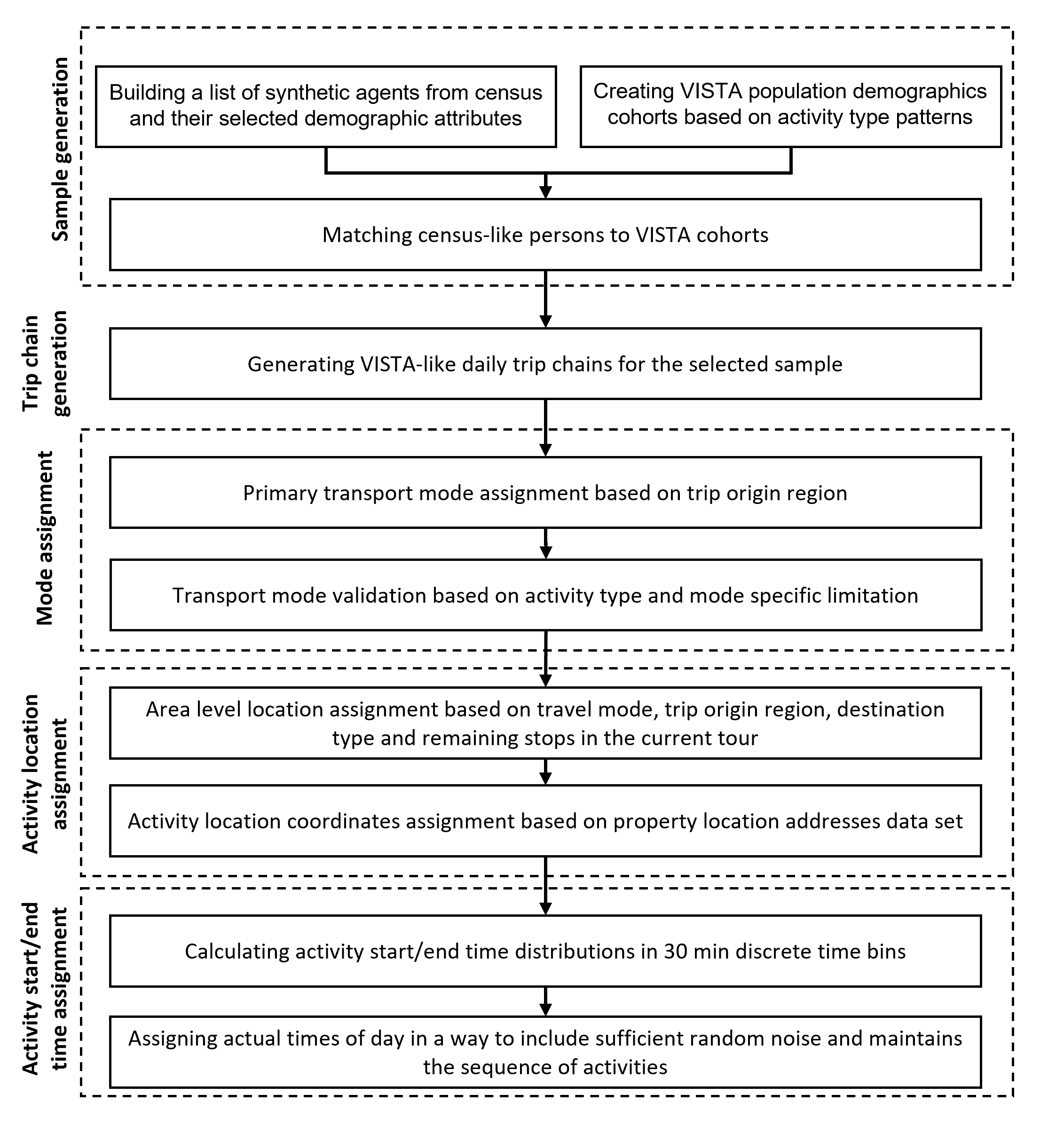
Figure 1: Overview of the synthetic population generation method (Section 2).

The process is fully automated and has been optimised to parallelise aspects using multiple cores where available for speedup, making it suitable for use on desktop machines and high performance infrastructure alike. To give the reader an appreciation for computing requirements and run times, to build a 10% population sample for Greater Melbourne corresponding to 311,788 unique synthetic individuals with their full travel diaries took 16 hours and 23 minutes on our test machine with 16 cores (Intel i7-6900K 3.20GHz) and 32GB RAM.

The output of the algorithm is a Comma Separated Values (CSV) file containing the generated daily travel plans of the virtual population, in the form of travel diaries, not too dissimilar to the travel diaries provided in VISTA. An example generated diary is given in Table 1. The steps of the algorithm incrementally add data to the relevant header columns of the table, for all agents. What each column means, and how it is populated, is covered in subsequent sections.

Table 1: Example synthetic output travel diary generated by the algorithm presented in Section 2. The 13 data columns for the four activities of the person are wrapped around to fit the wide table on the page.

PlanId
161
161
161
161

Activity
Home
Study
Work
Home

StartBin
1
17
34
45

EndBin
17
34
45
48

AgentId
213021342P2848193
213021342P2848193
213021342P2848193
213021342P2848193

SA1
21302134204
21302134242
21302134115
21302134204

LocationType
home
education
work
home

Mode
NA
car
car
car

Distance
1519
2509
4028
NA

X
304992
305720
307321
304992

Y
5804707
5805729
5806231
5804707

StartTime
00:03:30
08:29:00
17:00:00
22:07:30

EndTime
08:07:00
16:54:00
22:02:00
23:50:00

We now describe the different parts of the process of Figure 1, that yields an output like that in Table 1, in detail.

2.1 Processing the VISTA Trip Table

The first step in building the activity-based virtual population for Greater Melbourne is to process the raw anonymized Victorian Integrated Survey for Travel and Activity (VISTA)2012-18 data made openly available by the Department of Transport. These data are provided in several Comma Separated Values (CSV)files. For this study we use what is known in the VISTA dataset as the Trip Table (provided in T_VISTA1218_V1.csv). The Trip Table contains anonymized data for 174270 trips, representing 49453 persons from 21941 households.

2.1.1 Understanding VISTA Trip Table data

Table 2 shows a sample of the Trip Table data for a household (id: Y12H0000104) of three members (ids: Y12H0000104P01, Y12H0000104P02, Y12H0000104P03). Here PERSID is the person ID number, ORIGPURP1 is Origin Purpose (Summary), DESTPURP1 is Purpose at End of Trip (Summary), STARTIME is Time of Starting Trip (in minutes, from midnight), ARRTIME is Time of Ending Trip (in minutes, from midnight), and WDTRIPWGT is Trip weight for an ‘Average weekday’ of the combined 2012-18 dataset, using the Australian Standard Geographical Classification (ASGC). For brevity, we focus the following discussion on an average weekday, but the technique is applied in precisely the same way for the ‘Average weekend day’ data rows, given by the corresponding WEJTEWGT column.

Table 2: Trips of an example household Y12H0000104 from the VISTA Trip Table

PERSID	ORIGPURP1	DESTPURP1	STARTIME	ARRTIME	WDTRIPWGT
Y12H0000104P01	At Home	Work Related	420	485	83.77
Y12H0000104P01	Work Related	Go Home	990	1065	83.77
Y12H0000104P02	At Home	Work Related	540	555	86.51
Y12H0000104P02	Work Related	Buy Something	558	565	86.51
Y12H0000104P02	Buy Something	Go Home	570	575	86.51
Y12H0000104P02	At Home	Buy Something	900	905	86.51
Y12H0000104P02	Buy Something	Go Home	910	915	86.51
Y12H0000104P03	At Home	Work Related	450	480	131.96
Y12H0000104P03	Work Related	Go Home	990	1020	131.96

Table 2 shows the complete set of Trip Table attributes that our algorithm uses to generate VISTA-like activity/trip chains. An important point to note here is that we completely disregard all geospatial information from the records, and focus only on the sequence of activities and trips. This is because our intent is to generate location-agnostic VISTA-like activity/trip chains initially, and then in subsequent steps of the algorithm place these activities and trips in the context of the geographical home location assigned to the virtual person. Also note that no information about the mode of transportation is retained at this stage. Again, this will be introduced in the context of the home location later in the process.

Figure 2: Ordered sequence of activities (circles) and trips (arrows) for anonymous person Y12H0000104P02 in the VISTA Trip Table

Figure 2 gives a visual representation of the sequence of activities and trips of the example person Y12H0000104P02 of Table 2 with each row of the table represented by a numbered arrow in the figure. Person Y12H0000104P02’s day could be summarised as: left home at 9am (540 minutes past midnight) and 15 minutes later performed a quick work related activity that lasted three minutes (maybe to the local post office?); went back home via a quick seven minute stop to buy something (a morning coffee perhaps?); stayed at home from 9:35am (575 minutes past midnight) to 3pm (900 minutes past midnight); did another quick 15 minute round trip to the shops; then stayed home for the rest of the day.

The trips of sample person Y12H0000104P02 highlight some important choices that must be made when interpreting the data. For instance, did the person go to different shops (as we suggest in Figure 2) or the same one? Does the same assumption apply for all kinds of trips? In general, we apply the following rules to multiple trips for the same kind of activity during the day.

• All trips that start and end at a home related activity (ORIGPURP1 or DESTPURP1 contains the string ‘Home’) are assumed to be associated with the same home location.

• All sub-tours (sequences of activities starting and ending at home, such as the morning and afternoon sub-tours of person Y12H0000104P02) that contain multiple work-related trips are assumed to be associated with a single work location, however the work locations between two sub-tours are allowed to be different.

• All other trips (including shopping related trips) are assumed to be potentially associated with different locations, even if performed within the same sub-tour.

2.1.2 Extracting daily activities from Trip Table

Each row of Table 2 gives the start and end time of a single trip, and it is easy to see that the difference between the start time of one trip and the end time of the preceding trip of the person is in fact the duration of the activity between those two trips. The first trip in the chain does not have a preceding activity of course, but here the concluding activity can safely be assumed to have a start time of midnight. This knowledge can therefore be used to transform the trips-table into a corresponding activity-table. Table 3 shows this transformation for the trips of our sample household.

Table 3: Activities of example household Y12H0000104 derived from Trip Table

PERSID	ACTIVITY	START.TIME	END.TIME	WDTRIPWGT
Y12H0000104P01	At Home	0	420	83.77
Y12H0000104P01	Work Related	485	990	83.77
Y12H0000104P01	Go Home	1065	1439	83.77
Y12H0000104P02	At Home	0	540	86.51
Y12H0000104P02	Work Related	555	558	86.51
Y12H0000104P02	Buy Something	565	570	86.51
Y12H0000104P02	At Home	575	900	86.51
Y12H0000104P02	Buy Something	905	910	86.51
Y12H0000104P02	Go Home	915	1439	86.51
Y12H0000104P03	At Home	0	450	131.96
Y12H0000104P03	Work Related	480	990	131.96
Y12H0000104P03	Go Home	1020	1439	131.96

The activities table thus produced for the entire Trip Table then provides the raw input that forms the basis for our activity-based plan generation algorithm.

2.1.3 Simplifying activity labels

The number of unique activity labels present in the activity-table derived in the previous step is reduced by grouping related labels into simpler tags. We also rename some labels for clarity. Table 4 shows the specific text replacements that we perform in the ACTIVITY column of our activity-table from the previous step. The resulting activity-table has $\mathcal{A}$ unique activity types, being: Home, Mode Change, Other, Personal, Pickup/Dropoff/Deliver, Shop, Social/Recreational, Study, With Someone, Work.

Table 4: Label simplification performed on the Trip Table derived activity names

Original Trip Table label	Replacement label
At Home ; Go Home ; Unknown Purpose (at start of day)	Home
Social ; Recreational	Social/Recreational
Pick-up or Drop-off Someone ; Pick-up or Deliver Something	Pickup/Dropoff/Deliver
Other Purpose ; Not Stated	Other
Personal Business	Personal
Work Related	Work
Education	Study
Buy Something	Shop
Change Mode	Mode Change
Accompany Someone	With Someone

2.1.4 Calculating activity start/end time distributions in $\mathcal{T}$ discrete time bins

The final step in the VISTA data processing is to calculate the start and end time distributions for each activity type throughout the day–where the day is split into $\mathcal{T}$ discrete time bins of equal size. The parameter $\mathcal{T}$ gives a way of easily configuring the desired precision of the daily plan generation step of the algorithm (Section 2.4). Higher values of $\mathcal{T}$ allow the algorithm to seek higher precision in the generated activity start/end times but can lead to more variance in error, while lower values seek coarser precision which is easier to achieve resulting is lower error. What value gives a good balance between accuracy and error can be determined from experimentation. In this work, we use $\mathcal{T}$ $=48$, i.e., we break up the day into 48 time bins of 30 minutes each.

Figure 3: Structure of matrix $\mathcal{D}$ for storing start(end) time distributions for $|\mathcal{A}|$ activities against $\mathcal{T}$ time bins of the day

Calculation of the activities’ start(end) time distribution is done by first counting, for each activity, the number of instances of activity start(end) in every time bin. To do this, we create a matrix $\mathcal{D}$ (being $\mathcal{D}_{s}$ for start time distributions and $\mathcal{D}_{e}$ for end time distributions) with $\mathcal{A}$ rows of unique activity types and $\mathcal{T}$ columns for every time bin (Figure 3). Then for every row $r$ in the activity-table, we update the value of the corresponding cell in $\mathcal{D}$, given by the $\mathcal{D}$-row that matches the ACTIVITY label in $r$ and the $\mathcal{D}$-column corresponding to the time bin for the start(end) time of the activity in $r$. The value of this determined cell is then incremented by the value of the WDTRIPWGT column in $r$, which gives the frequency of this activity in the full population (remembering that the VISTA Trip Table represents a 1% sample). We save this output in CSV format, to be used by subsequent steps of the algorithm. Note that the end-time distribution table $\mathcal{D}_{e}$ saved has $\mathcal{A}$ $\times$$\mathcal{T}$ rows, since we save the end time for every activity type (Table 4) for every start time bin. In other words, for end times, we store $\mathcal{T}$ matrices of the type shown in Figure 3.

Figure 4 shows a consolidated view of the simplified activities of the Melbourne population across the day split into $\mathcal{T}$ $=48$ discrete time bin distributions, computed separately for the weekday and weekend rows of the activity-table we derived from Trip Table. Each split bar shows the proportion of the population performing the different activities in $\mathcal{A}$ during the corresponding time bin.

Figure 4: Simplified VISTA Trip Table derived activities in $\mathcal{T}$ $=48$ discrete time bins

2.1.5 Generating VISTA population cohorts

The process explained so far in Section 2.1 shows how the VISTA Trip Table, bar weekend trips, is used to compute distributions of activities in discrete time bins of the day. We now describe a slight modification to the process, to account for differences in activity profiles across population subgroups, or cohorts.

It is well understood that the kinds of activities people do can be shaped by individual, social, and physical factors Bautista-Hernández, (2020); Grue et al., (2020). Not all of these will be known and/or related variables available in the VISTA data. Nevertheless, it is clear that some steps can be taken to classify observed behaviours into groups given the variables we do have.

We implemented a simple classification based on the demographic attributes of gender and age, to find distinct groupings that exhibit significantly distinct trip patterns. Specifically, participants were broken into five year age groups, with the exception of groups 0-14 and 65 and over. Probabilities for the activities Work, Study, Shop, Personal, and Social/Recreational were then calculated for each of these 24 groups based on weekday trips. Hierarchical clustering was then applied to the dataset using Ward’s method, producing the dendrogram shown in Figure 5.

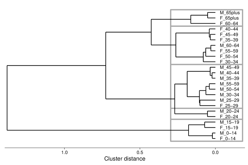
Figure 5: Dendrogram of hierarchical cluster analysis. Grey rectangles indicate clusters.

The gap statistic of the clustering process indicated that five unique groupings would be optimal. The output of the classification is the gender and age range of those identified groups. Our final step then was to filter the VISTA Trip Table records on those attributes and store the result as partial tables, one per group. The process described so far in Section 2.1 was therefore applied to each partial trip table separately rather than the VISTA Trip Table directly–as suggested earlier to keep the explanation simple–giving activity distribution tables by time of day per subgroup.

2.2 Creating a representative sample of census-like persons

This step of the algorithm is concerned with allocating the right kinds of persons to the right statistical areas in Greater Melbourne as per Australian Census 2016. The output of this step is a list of uniquely identified synthetic persons, each described by a valid street address representing their home location, and demographic attributes of age and gender that, when aggregated, match the demographic distributions reported in the census at the SA2 level.

A full virtual population for Greater Melbourne based on ABS Census 2016 was created by Wickramasinghe et al., (2020). Their output population is made available through their GitHub code repository. It consists of a relational database of unique persons in unique households assigned to known street addresses. For convenience, their database is supplied in two CSV files containing persons and households respectively, separately for each of the 307 SA2 areas in Greater Melbourne.

We obtain our census-based synthetic individuals by simply sampling a desired number of persons from Wickramasinghe et al., (2020)’s population files. So, for instance, to build a 10% sample of the Greater Melbourne population, we randomly sample 10% persons from each of the 307 SA2 level persons CSV files provided. This gives us our base census-like individuals at home locations in Greater Melbourne. Subsequent steps assign VISTA-like trips to these persons, representing the kinds of trips persons of their demographic makeup in the given SA2 undertake in their day as per VISTA data.

2.3 Matching census-like persons to VISTA cohorts

In this step of the algorithm we assign, to the census-like persons from the last step (Section 2.2) and based on their demographic profile, one of the VISTA groups, or cohorts, calculated previously (Section 2.1.5). This is required so that in the subsequent step we can apply group-appropriate trip generation models for assigning representative trips and activities to those individuals.

The matching of persons to cohorts itself is a straightforward process. Since each cohort is fully defined by a gender and age range, then the cohort of a person can be determined by a simple lookup table. The output of this step is the addition of a new attribute to each person, indicating the cohort they belong to.

In the final output of the algorithm, as shown in Table 1, this step is responsible for populating column AgentId, that gives a unique identifier for a synthetic census-like person sampled in the earlier step (Section 2.2), and was matched to the VISTA-like activity chain given by column PlanId.

2.4 Generating VISTA-like daily trips

The algorithm described here does not discuss groups, however the reader should keep in mind that the process being described is applied separately to the cohorts identified in Section 2.1.5.

Algorithm 1 gives the pseudo-code of our algorithm for generating VISTA-like activity chains. The objective of the algorithm is to generate a sequence of $\mathcal{N}$ activity chains in such a way that, when taken together, the list $\mathcal{C}$ of generated activity chains achieves the target activity start(end) time distributions given by the $\mathcal{D}$-matrices $\mathcal{D}_{s}$ and $\mathcal{D}_{e}$. Here, the rows of the $\mathcal{D}$-matrices give the activities and the columns give their distribution over the time bins of the day.

The general intuition behind the algorithm is to repeatedly revise the desired distributions by taking the difference $\Delta$ between the presently achieved distributions ($\acute{\mathcal{D}_{s}}$ and $\acute{\mathcal{D}_{e}}$) and the target distributions ($\mathcal{D}_{s}$ and $\mathcal{D}_{e}$) so that over-represented activities in a given time bin are less likely to be generated in subsequent iterations while under-represented activities become more likely. This allows for dynamic on-the-fly revision so that the algorithm is continuously looking to correct towards the moving target distributions with every new activity chain it generates. This approach works well in adapting output to the target $\mathcal{D}$-matrices, and the generation error decreases asymptotically as the number $\mathcal{N}$ of generated activity chains increases.

Input : Activity start time distribution matrix $\mathcal{D}_{s}$, activity end-time distribution matrix $\mathcal{D}_{e}$, number of time bins $\mathcal{T}$, number of trip chains to generate $\mathcal{N}$

Output : Set of generated trip chains $\mathcal{C}$

1 // Init list $\mathcal{C}$ for storing generated trip chains

2 // Init matrix $\acute{\mathcal{D}_{s}}$ for storing start-time distributions of chains in $\mathcal{C}$

3 // Init matrix $\Delta$ for the difference from expected start time distributions

4 for $n\leftarrow 1$ to $\mathcal{N}$ do

5       // normalise to 1 all rows in $\Delta$ that have non-zero values

6       $\Delta\leftarrow\mathcal{D}_{s}-\Delta$;

7        // get the difference from expected

8       // make $\Delta$ rows $\geq 0$ by adding the minimum value of each row as offset

9       // for every zero-cell in $\mathcal{D}_{s}$ make the corresponding cell in $\Delta$ zero

10       // re-normalise to 1 all rows in $\acute{\mathcal{D}_{s}}$ that have non-zero values

11       $b\leftarrow 1$ ;

12        // start at time bin 1

13       // Init list $\Phi$ for storing a new trip chain

14       while $b<$$\mathcal{T}$ do // while not at the final time bin

15             $p\leftarrow$Sum($\mathcal{D}_{s}[,b]$)/Sum($\mathcal{D}_{s}$);

16              // get % of activities that should start in $b$

17             $\acute{p}\leftarrow$Sum($\acute{\mathcal{D}_{s}}[,b]$)/Sum($\acute{\mathcal{D}_{s}}$);

18              // get % of activities starting in $b$ so far

19             if $\acute{p}>=p$ then // have more than the required share of starts for $b$

20                  // increment b and skip to start of loop

21                  

22             end if

23            $\delta\leftarrow\Delta[,b]$;

24              // pick the difference probabilities for time bin b

25             // set all zero-cells in $\delta$ that are non-zero in $\mathcal{D}_{s}[,b]$ to 0.001

26             // if all $\delta$ cells are zero then increment b and go to start of loop

27             // normalise $\delta$ to 1

28             // use $\delta$ values to probabilistically select an activity $a$ from $\mathcal{A}$

29             $b_{s}\leftarrow b$;

30              // set the start bin for activity $a$

31             // from $\mathcal{D}_{e}$ get the row $\gamma$ for activity $a$ starting in bin $b_{s}$

32             // if $\gamma$ has all cells zero, then set all cells to 1

33             // use $\gamma$ values to probabilistically select an end bin $b_{e}$ for $a$

34             // append list $[a,b_{s},b_{e}]$ to the end of $\Phi$

35             $b\leftarrow b_{e}$;

36              // skip to the bin that activity $a$ finished on

37            

38       end while

39      // if $\Phi$ is empty then append list $[Home,1,\mathcal{T}]$ to it

40       // collapse consecutive blocks of the same activity in $\Phi$ into one

41       // append $\Phi$ to the end of $\mathcal{C}$

42       $\acute{\mathcal{D}_{s}}[a,b_{s}]\leftarrow\acute{\mathcal{D}_{s}}[a,b_{s}]+1$;

43        // increment the count for $a$ starting in $b_{s}$

44      

45 end for

Algorithm 1 Algorithm for generating VISTA-like activity chains

We describe in Algorithm 1 the steps for matching to the target start time distribution matrix $\mathcal{D}_{s}$ and note that the steps are the same for matching to the end time distribution matrix $\mathcal{D}_{e}$. The process starts by initialising an empty list $\mathcal{C}$ for storing the activity chains to generate, a corresponding empty matrix $\acute{\mathcal{D}_{s}}$ for recording the start-time distributions of the activities in $\mathcal{C}$, and another empty matrix $\Delta$ for storing the difference from the target distributions in $\mathcal{D}_{s}$ (lines 1–3). Both $\acute{\mathcal{D}_{s}}$ and $\Delta$ have the same dimensions as $\mathcal{D}_{s}$ as shown in Figure 3. The following steps (lines 4–34) are then repeated once per activity chain, to generate $\mathcal{N}$ activity chains.

Prior to generating a new activity chain, the difference matrix $\Delta$ is updated to reflect the current deviation from the desired distribution $\mathcal{D}_{s}$ (lines 5–9), ensuring that zero-value cells in $\mathcal{D}_{s}$ are also zero-value in $\Delta$, and normalising the row vectors to lie in the range [0,1]. This means that any zero-value cells in $\mathcal{D}_{s}$ are either so because the activity (row) does not occur in that time bin (column), or the proportion of the given activity in the given time bin for the population generated thus far either perfectly matches the desired or is over-represented. On the other hand, values tending to $1.0$ indicate increasing levels of under-representation.

The algorithm then traverses the time bins sequentially from beginning of the day to end (line 10, 12) as follows. We first check if the proportion of activities, across all activities, that start in the current time bin, is already at or above the desired level, and if found to be so we skip to the next time bin (lines 13–17). Otherwise we extract from $\Delta$, a vector $\delta$ to give, for the current time step, the difference from desired for all activities (line 18). If $\delta$ is zero because it is also zero in the desired distribution $\mathcal{D}_{s}$ then we skip to the next time bin (lines 19–20), else we use $\delta$ to probabilistically select a corresponding activity and set its start time to the current time bin (lines 22–23). This procedure results in a higher chance of selection of under-represented activities. The end time for the selected activity is chosen probabilistically from the probabilities of the given activity ending in the remaining time bins of the day, when starting in the current time bin (lines 24–26). The generated activity with its allocated start and end bins is added to the trip chain $\Phi$ (line 27) and we skip to the activity end time bin (line 28) to continue building the chain.

The trip chain $\Phi$ thus generated is compressed by collapsing consecutive blocks of the same activity into a single activity that starts in the time bin of the first occurrence and finishes in the time bin of the last (line 31). If $\Phi$ was empty to begin with, i.e., no activity was generated in the preceding loop, then we just assign a $Home$ activity lasting the whole day (line 30). The trip chain $\Phi$ is then added to our list $\mathcal{C}$ (line 32). Finally, the counts of the generated activities en $\Phi$ are incremented in $\acute{\mathcal{D}_{s}}$, to be used do update the difference matrix $\Delta$ before generating the next activity chain.

In the final output of the algorithm, an example of which is given in Table 1, this step is responsible for populating columns PlanId (a unique identifier for the generated activity chain), Activity (the sequence of activities in the chain), StartBin (the start time bin for each activity, being an integer between 1 and 48, representing the 30-minute blocks of the day), and EndBin (the corresponding end time bins for the activities).

2.5 Assigning statistical areas (SA1) to activities

At this point, each agent now has a home Statistical Area level 1 (SA1) and a list of activities they conduct throughout the day. Candidate locations for these activities were selected from the endpoint nodes of non-highway edges (i.e., edges with a speed of 60km/h or less and accessible by all modes) of the OSM-derived transport network generated by (cite network paper here). It is important to note that these non-highway edges were already densified, with additional nodes added every 500 meters. These locations were selected to ensure that any activity location would be reachable from the network without any non-network travel movement (i.e. bushwhacking). These locations were then classified according to the land use category of the mesh block they lie within. In order to facilitate matching location types to activity types, the mesh block categories were simplified into five types: Home, Work, Education, Commercial, and Park (see Table 5).

Table 5: VISTA category reclassification

Location categories	Meshblock categories	VISTA activities
Home	Residential, Other, Primary Production	Home
Work	Commercial, Education, Hospital/Medical, Industrial, Primary Production	Other, Pickup/Dropoff/Deliver, With Someone, Work
Education	Education	Other, Pickup/Dropoff/Deliver, Study, With Someone
Commercial	Commercial	Other, Personal, Pickup/Dropoff/Deliver, Shop, Social/Recreational, With Someone
Park	Parkland, Water	Other, Pickup/Dropoff/Deliver, Social/Recreational, With Someone

Transport mode is then assigned sequentially to each trip, along with SA1 region to non-home activities. The specifics detailed in Algorithm 2, but broadly, transport mode is selected first. This then allows for region selection based on the likely travel distance for that mode, as well as the relative attractiveness of potential destinations for the chosen trip purpose.

1

Input/Output : Activity table $A=\langle AgentId:\mathbb{N},Region:\mathbb{N}\cup\varnothing,\newline LocationType:\{home,work,education,commercial,park\},\newline ArrivingMode:\{walk,cycle,pt,car,\varnothing\}\rangle$

2

3// Init $anchor\_region\leftarrow\textnormal{{FALSE}}$

4 // Init $primary\_mode\leftarrow\varnothing$

5

6for $i\leftarrow 1$ to $\mathcal{N}$ do

7       if $LocationType_{i}=home$ AND $LocationType_{i+1}\neq home$ then

8             $anchor\_region\leftarrow\textnormal{{FALSE}}$ ;

9             $primary\_mode\leftarrow\textnormal{{getMode}}(Region_{i})$ ;

10             $ArrivingMode_{i+1}\leftarrow primary\_mode$ ;

11             $Region_{i+1}\leftarrow getRegion(Region_{i}$, $LocationType_{i+1}$, $primary\_mode$, $homeCount(i))$ ;

12             $ArrivingMode_{i+\textnormal{{homeCount}}(i)}\leftarrow primary\_mode$ ;

13            

14      else

15             if  $LocationType_{i}\neq home$ AND $(homeCount(i)>2$ OR $(homeCount(i)=2$ AND $primary\_mode\in\{walk,pt\}))$ then

16                   $ArrivingMode_{i+1}\leftarrow\textnormal{{getMode}}(Region_{i}$, $primary\_mode$, $anchor\_region)$ ;

17                  

18                  if $anchor\_region=\textnormal{{FALSE}}$ AND $primary\_mode\in\{bike,car\}$ AND $ArrivingMode_{i}\neq ArrivingMode_{i+1}$ then

19                         $Region_{i+\textnormal{{homeCount}}(i)-1}\leftarrow Region_{i}$ ;

20                         $ArrivingMode_{i+\textnormal{{homeCount}}(i)-1}\leftarrow ArrivingMode_{i+1}$ ;

21                         $anchor\_region=\textnormal{{TRUE}}$ ;

22                        

23                   end if

24                  if $primary\_mode=walk$ AND $ArrivingMode_{i+1}=pt$ then

25                         $ArrivingMode_{i+\textnormal{{homeCount}}(i)}\leftarrow pt$ ;

26                        

27                   end if

28                  if $anchor\_region=\textnormal{{TRUE}}$ then

29                         $Region_{i+1}\leftarrow getRegion(Region_{i}$, $LocationType_{i+1}$, $ArrivingMode_{i+1}$, $homeCount(i)-2)$ ;

30                        

31                  else

32                         $Region_{i+1}\leftarrow getRegion(Region_{i}$, $LocationType_{i+1}$, $ArrivingMode_{i+1}$, $homeCount(i)-1)$ ;

33                        

34                   end if

35                  

36             end if

37            if $Region_{i}\neq home$ AND $homeCount(i)=2$ AND $primary\_mode\in\{bike,car\}$ AND $anchor\_region=\textnormal{{FALSE}}$ then

38                   $ArrivingMode_{i+1}\leftarrow ArrivingMode_{i}$ ;

39                   $Region_{i+1}\leftarrow getRegion(Region_{i}$, $LocationType_{i+1}$, $primary\_mode$, $homeCount(i)-1)$ ;

40                  

41             end if

42            

43       end if

44      

45 end for

Algorithm 2 Algorithm for assigning transport mode and SA1 region to trips

2.5.1 Mode selection

Transport mode selection is taken care of by the getMode function, which selects from the possibilities of walk, bike, pt (public transit), or car. This function takes the current region as input to ensure that local variation in mode choice is present in the agents’ behavior. Specifically, some modes, such as walking and public transit are more popular towards the inner city, whereas driving is preferred by residents of the outer suburbs.

The first run of the function for each agent sets their primary mode, which is the initial mode used when an agent leaves home. Primary mode is used as an input of the getMode function to ensure vehicle use (i.e., car or bike) is appropriate. Specifically, if a vehicle is not initially used by an agent, then it is not possible to select one at any other point throughout the day. It is however possible for agents to switch from a vehicle to walking or public transit. To prevent agents leaving vehicles stranded, they must return to that region so they may use the vehicle to return home. Additionally, walking and public transit my be freely switched between, so long as the final trip home utilizes public transit.

The mode choice probabilities used by the getMode function were generated for each SA1 region by analyzing the proportions of modes chosen by the participants of the VISTA travel survey. For this, the full travel survey was used, meaning that origin (ORIGLONG, ORIGLAT) and destination (DESTLONG, DESTLAT) coordinates were available. Trips were filtered to weekdays (using TRAVDOW) within the Greater Melbourne region and were recorded with their origin location, survey weight (CW_WDTRIPWGT_SA3), and transport mode (LINKMODE, which was reclassified to match the virtual population. Survey weight is a number that indicates how representative each entry is of the Victorian population during a weekday, and was used in calibrating accurate mode choice proportions. To determine mode the proportions, Kernel Density Estimation (KDE) was calculated at each candidate location for each transport mode, using a weighted Gaussian kernel with a bandwidth of 750 meters, to be aggregated up to SA1 and converted to a percentage. Destination locations were used instead of creating a density raster as it is much faster to compute, and only produces density calculations at places agents are able to travel.

Selecting an appropriate bandwidth for density calculations is important as smaller bandwidths show greater local variation but have fewer points to use, and larger bandwidths use more points, but show more general trends. In this case, 750 meters was chosen based on calibration. Specifically, a variety of potential bandwidths were chosen, with their mode choice percentages aggregated to Statistical Area level 3 (SA3) regions. These percentages were then compared to values obtained by aggregating the weighted VISTA mode choice proportions to SA3 region in order to select the bandwidth with the best fit. SA3 regions were chosen for calibration as that is the statistical granularity the VISTA travel survey was weighted at.

2.5.2 Destination selection

Selection of a destination region is handled by the getRegion function, which uses the current region, the location type of the destination region, the current mode, and the number of trips remaining until the home region is reached (hop count). Because trips with multiple stages tend to move further away from the home region, the remaining leg home can be unnaturally long. Hop count was used to filter candidate destination regions down to ones where it would be likely to for that mode, based on the number of trips remaining to get home assuming 95th percentile trip lengths based on their distance distribution. This was to ensure that the final trip home will not be unreasonably long, which can be a particular issue for walking trips. The getRegion function is primarily a trade-off between selecting a destination that is a likely distance for the mode selected, and the attraction of the destination. Figure 6 illustrates how the distance distribution and destination type probabilities are combined to create the probabilities needed to select the next region.

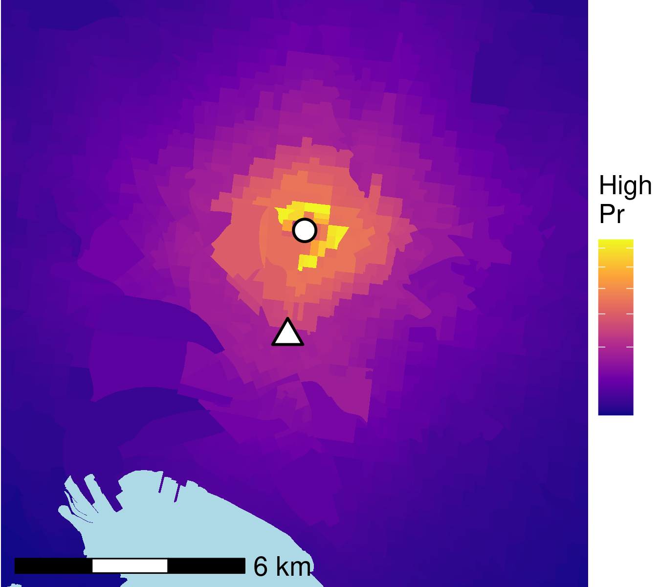
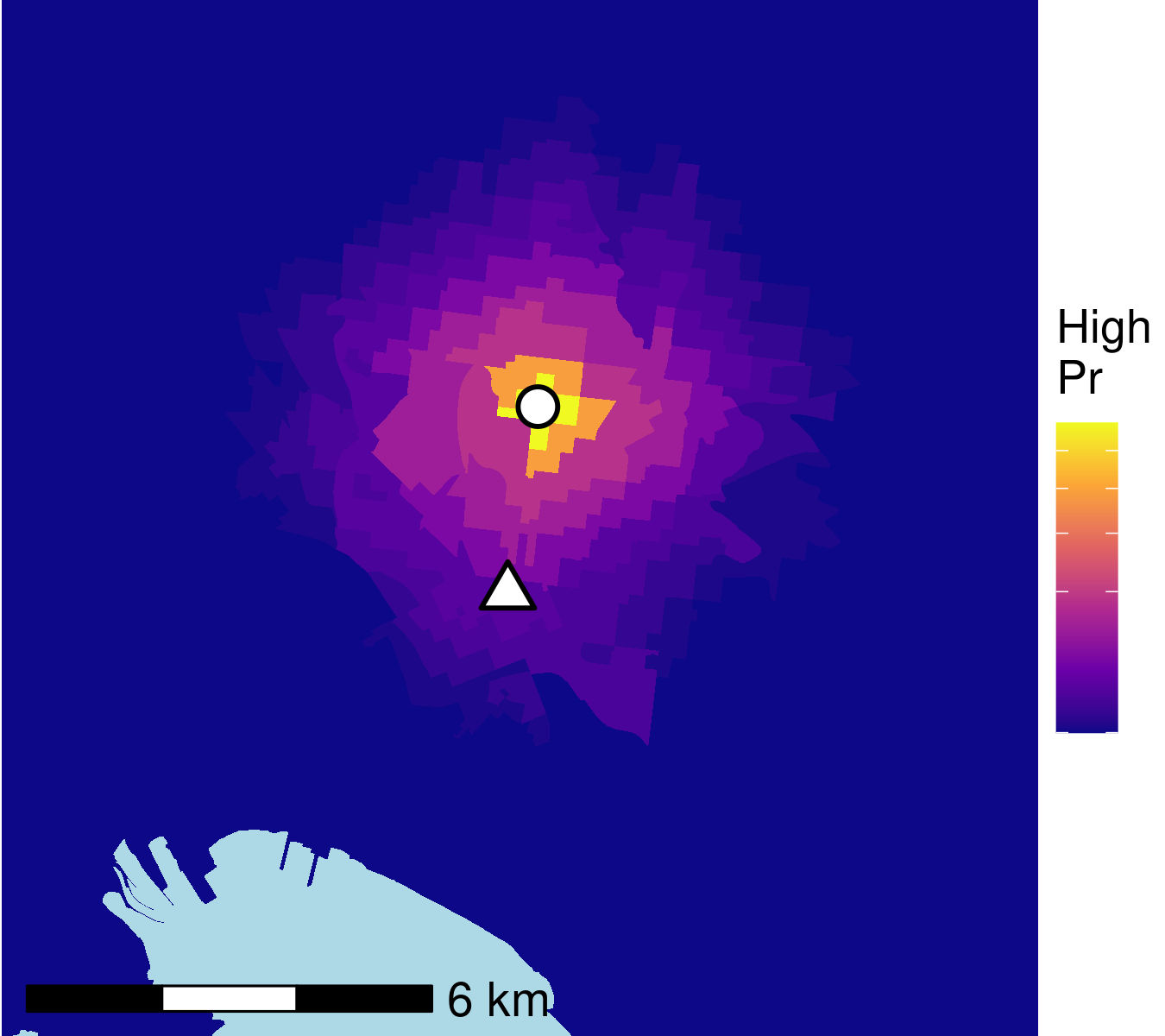
(a)	(b)
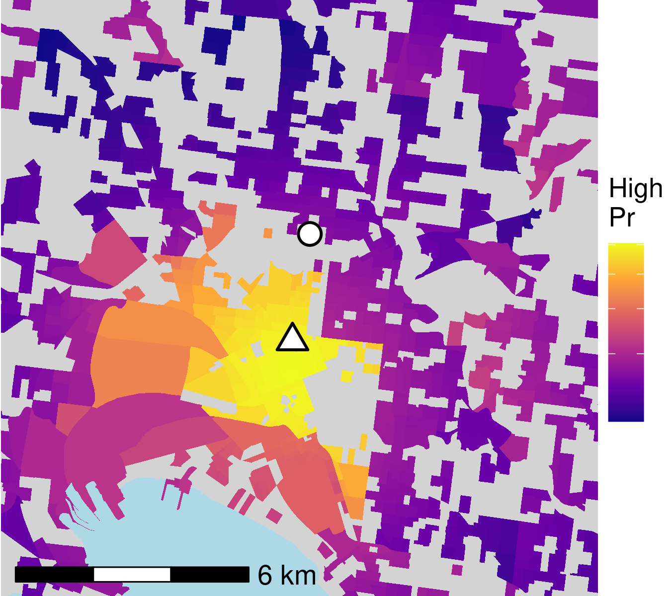
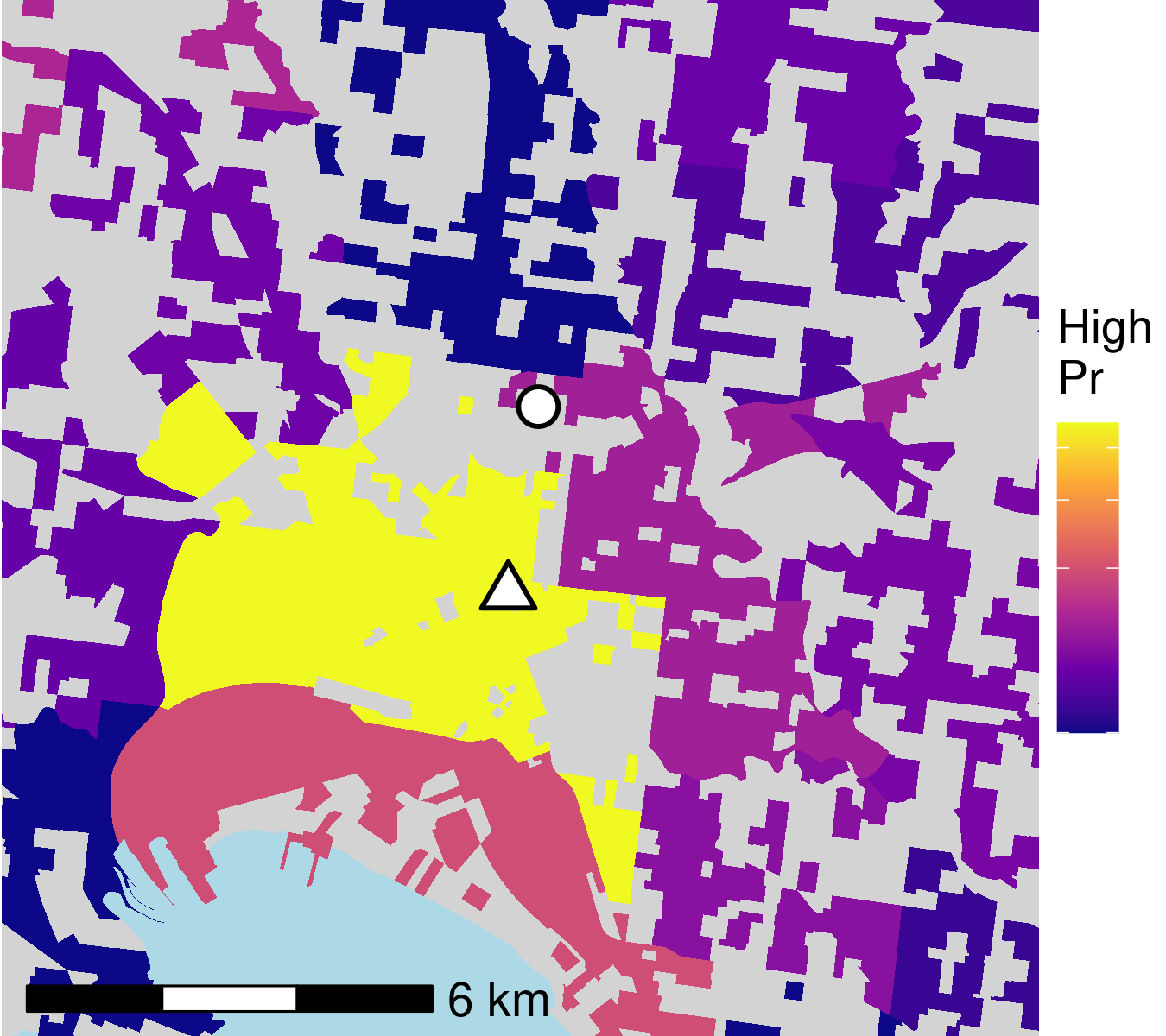
(c)	(d)
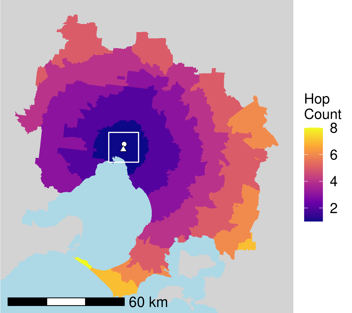
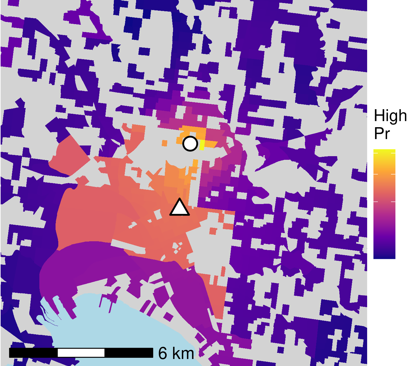
(e)	(f)

Figure 6: Selecting next region for a cycling trip from home (circle) to work (triangle) showing: region selection probability (Pr) for local and global distance distributions (a and b), region selection probability (Pr) for local and global destination attraction (c and d), number of trips (hop count) that would be reasonably required to reach home (e), and combined region likelihood (f).

In order to provide a set of distances for the algorithm to choose from, an origin-destination matrix was calculated between the population-weighted centroids of ABS SA1 regions using the OSM-derived transport network. Population-weighted centroids were used as they are more representative of regions with uneven population distributions, and were calculated using the centroids of the ABS meshblocks with their 2016 census population. The SA1 centroids were then snapped to the nearest non-highway node and the shortest distance was calculated between all locations to populate the OD matrix.

To calculate a distance distribution for each SA1 region, the population-weighted centroid was used as a base, selecting the closest 500 VISTA trips for each transport mode. A weighted log normal distribution was then calculated for each transport mode and centroid, recording their log-mean and standard deviation. The log-normal distribution was chosen as it better fit the distances than a normal distribution as there are no negative distances and can better exhibit a sharp peak at low distances regardless of transport mode.

While it would be preferable to use a distance-based bandwidth as in the previous section to select trips to build the distributions, accurate representation of distributions requires more data than density-based measures. The closest 500 trips were chosen instead as only driving, with its 67,769 trips, was able to build representative distributions, whereas there were only 14,621 walking, 7,166 public transport, and 1,515 cycling trips. These distributions were calculated at the population-weighted centroids instead of the destination locations as the variation within the SA1 regions was not significant enough to warrant the additional computation costs.

Calculating the distance probabilities was performed by first filtering the OD-matrix to the current SA1 region, providing a set of distances to all other regions. The log-mean and standard deviation for the chosen transport mode for the region was then used to filter potential destinations to only those with distances within the 5th and 95th percentile of the log-normal distribution, ensuring unlikely distances would not be selected. Potential destinations where the attraction probability was zero were also filtered to ensure that there would be a suitable destination location present. Probabilities were then calculated for the remaining destinations based on their distances and the log-mean and standard deviation for the nominated transport mode. These were then normalized so that their total equaled one. Because there are far fewer short distances than longer distances, the probabilities were further normalized by binning distances into 500 meter categories and then dividing each probability by the number of distances in that category.

Destination attraction was calculated similar to mode probability, with the probabilities retrieved for the nominated destination category. Kernel Density Estimation (KDE) was again calculated at each candidate location for each destination category, using a weighted Gaussian kernel with a bandwidth of 3,200m for work, 300m for park, 200m for education, and 20,000m for commercial destinations. These were then aggregated up to SA1 and converted normalized so that the total attraction value equaled one for each category.

Bandwidth selection was again based on calibration, where a variety of bandwidths were chosen, with the mode choice percentages aggregated to SA3 regions. These percentages were then compared to values obtained by aggregating the weighted VISTA trips by destination category to SA3 region in order to select the bandwidth with the best fit for each destination category.

While these criteria ensure that regions are selected that are locally representative, it is also important to ensure that the virtual population is representative for all of Greater Melbourne. To account for this, distance distributions and destination attraction were tallied at the SA3 level, so that the destination region could also be selected based on how well it would improve the fit of the overall distributions. For example, the distances of previous cycling trips have been on average longer than the expected distribution. To account for this, in Figure 6 the global distance probability is more likely to choose distances that are shorter than the local distance probability. This is also the case for destination attraction, where a higher probability has been placed on the inner city as an insufficient number of work trips have been arriving there.

The final combined probability was then calculated by filtering the candidate regions to those within the hop count, and then adding the local distance and destination attraction probabilities to the global distance and destination attraction probabilities, normalising the probabilities so that their total equaled one. From this point, a location could then be selected, as illustrated in Figure 6.

In the final output of the algorithm (Table 1), this step is responsible for populating columns SA1 (SA1 where this activity will take place), LocationType (the type of location within the SA1 where the activity should take place, to be assigned in the subsequent step), Mode (the travel mode by which the person will arrive at that activity; not applicable for the first activity of the day), and Distance (the distance between the current and preceding SA1 regions derived from the OD-matrix).

2.6 Assigning locations to activities in statistical areas

Now that an SA1 region has been assigned for every stop, location coordinates can be assigned based on the SA1 region and stop category. It is important to note that all home stops for an agent must share the same location. Locations are drawn from the set of candidate locations, which are points on the transport network that agents may move between.

For the same destination category and SA1 region, certain locations will always be more popular than others. For example, an office tower will have more employees, and therefore be a more attractive work destination, than single building. To account for this, addresses were selected from Vicmap Address, a geocoded database of property locations supplied by the Victorian government (Vicmap Address) containing 2,932,530 addresses within the Greater Melbourne region. These were then assigned a land use category based on the meshblock they were located within. In cases of meshblocks without any addresses within their boundaries, a single address was assigned at their geometries’ centroid.

In order to reduce the number of unique locations, the addresses were then snapped to the set of candidate locations mentioned in Section 2.5, which are points on the transport network that agents may move between. The address counts were then used to create a selection probability by normalizing their number by SA1 region and destination category so that their total equaled one. This probability was then used to assign locations to each stop.

In the final output of the algorithm (Table 1), this step is responsible for populating columns X and Y, representing the spatial coordinates of the location of activities, in the coordinate reference system of the input spatial data.

2.7 Assigning start and end times to activities

The final step of the algorithm converts the start and end times of activities, allocated initially at the coarse granularity of 30-min time bins (in Section 2.4), into actual times of day. The main considerations in doing so are to (a) add some random noise so that start/end times are sufficiently dispersed within the 30-min duration of each time bin; and (b) ensure that start/end times are ordered correctly so that activities do not end before their start, and activities do not start before the previous ones ends. This latter constraint becomes important where several starts and ends are being scheduled in the same time bin.

The method for achieving the desired time schedule is relatively straightforward. We first extract, for each person, the ordered vector of time bins corresponding to the sequence of start and end times for all activities. This is always a vector of even length, since every activity is represented by two sequential elements corresponding to its start and end. Further, this vector has values that increase monotonically, representing the progression time as sequential activities start and end in the person’s day. Next, this vector of time bin indices is converted to a time of day in seconds past midnight. We do this by taking the known start time of each time bin included in the vector and adding a randomly generated noise offset of a maximum duration of 30 minutes. This gives, across the population, start/end times evenly distributed within the time bins of activities. The obtained vector of times is then sorted in increasing order of numbers. This is necessary because the addition of random noise in the previous step can result in an out of order sequence of numbers within time bins where more than one activity is starting and/or ending. Sorting the vector rectifies any such issues and guarantees that the final ordering of start/end times are plausible and not mathematically impossible. Finally the time values, which represent offsets in seconds past midnight, are converted to a more convenient hh:mm:ss 24-hour format.

In the final output of the algorithm (Table 1), this step is responsible for populating columns StartTime and EndTime, representing the start and end times of activities in the day.

3 Results

This section compares a 10% sample size population generated by our process to the real-world observations of the VISTA travel survey in order to determine how well our model reflects the travel survey. In order to do so, the distance distributions (Section 3.1), destination attraction (Section 3.2), and mode choice (Section 3.3) of the synthetic population were analyzed. Additionally Section 3.4 compares synthetic populations of varying sizes to determine the effect of sample size on accuracy.

3.1 Distance distributions

Given that the synthetic population created by this work provides locations for each agent’s destination, but not routing information, distances will instead be calculated based on the distance between the SA1 regions provided by the OD-matrix of Section 2.5 (i.e., the shortest path distance along the road network between the population-weighted centroids of the two SA1 regions). To ensure consistency, the distances from the VISTA trips dataset were also replaced with the distance between SA1 regions.

Figure 7 shows the weighted expected distance distributions plotted alongside the actual distance distributions for the four transport modes. Fitted log-normal distributions are also plotted as dashed lines. In general, the actual distributions match the expected distributions closely, although the actual distributions appear to have larger values in the longer distances.

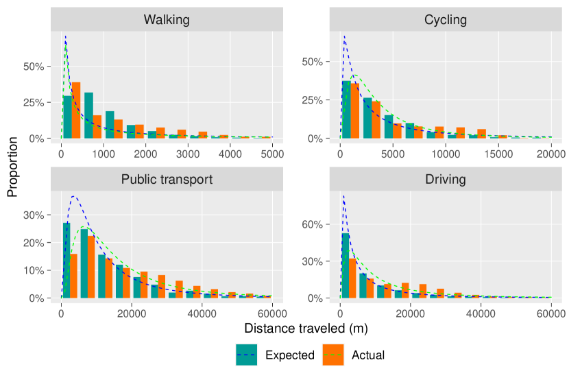
Figure 7: Distance histograms. Dashed lines represent the fitted log-normal distributions.

In order to determine if the spatial variation of the distance distributions was captured, actual and weighted expected distance distributions were aggregated to the 40 SA3 regions comprising Greater Melbourne. Figure 8 shows the log-normal and standard deviation of these distance distributions.

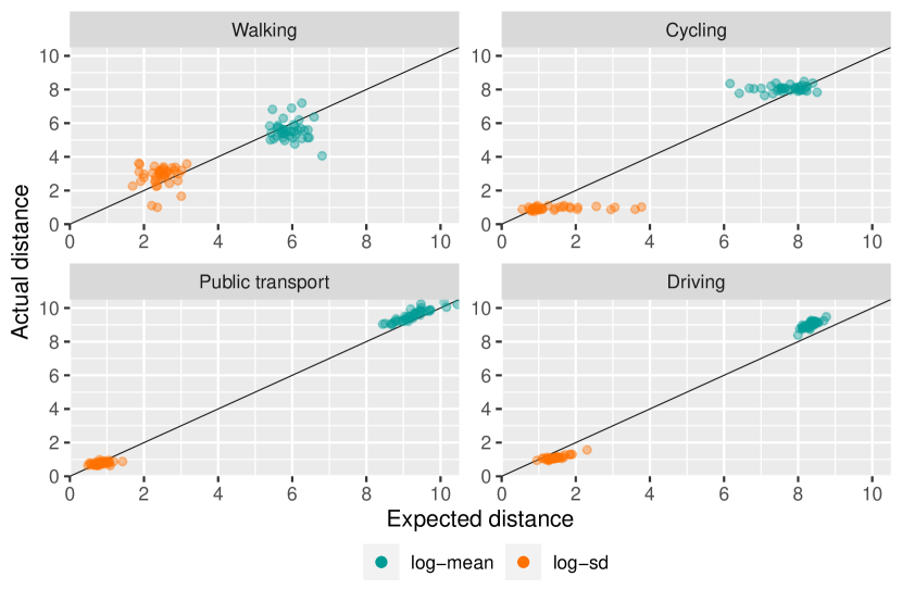
Figure 8: Expected versus actual distance distributions aggregated to SA3 regions.

Cycling appeared to have the largest variation, which is to be expected given that it is based on only 1,515 cycling trips. While walking had similar expected and actual values, there was little positive correlation. This is reasonable given that how far people are willing to walk likely has little to no spatial variation. In contrast, public transport and driving show far stronger positive correlation, meaning that the spatial variation of these modes is being captured. Additionally, the actual log-mean was on average smaller then the expected log-mean for driving and public transport, whereas the log-standard deviation was larger. This was consistent with Figure 7 given these modes tended to have a lower peak and longer tail in their histograms.

3.2 Destination attraction

In order to determine if the spatial variation of the destination activities were captured, Figure 9 compares actual and weighted expected destination probabilities aggregated to SA3 regions. It is important to note that the spatial variation of home locations was not plotted as the number of home locations for each SA1 is a value that is explicitly used when generating the synthetic population.

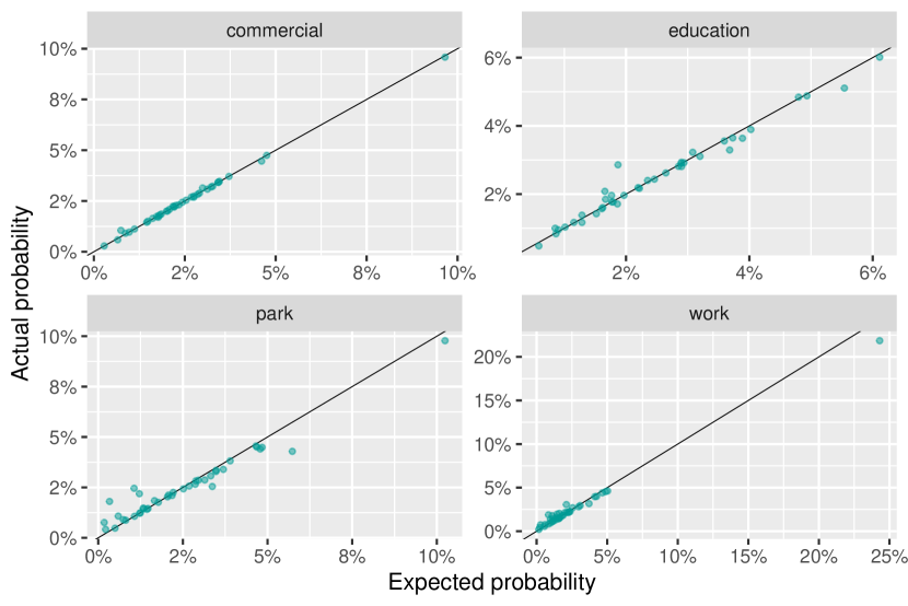
Figure 9: Expected versus actual destination probabilities aggregated to SA3 regions.

It is important to note that for commercial, park, and work activities, one of the SA3 regions has a much larger chance of being selected as it is the region containing Melbourne’s Central Business District (CBD). In general, SA3 regions had similar expected and actual probabilities regardless of destination type, indicating a good fit for destination selection. The park destination type did however display larger variation, likely due to being a comparatively unpopular activity and therefore having fewer trips. This was also the case to a lesser extent for the education activities. Additionally, all destination types displayed a large variance in probabilities along with a positive correlation, indicating that the spatial variation is being represented.

3.3 Mode choice

In order to determine if the spatial variation of the transport mode choice was captured, Figure 10 compares actual and weighted expected mode choice probabilities that were aggregated to SA3 regions.

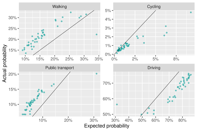
Figure 10: Expected versus actual mode choice probabilities aggregated to SA3 regions.

Walking, puplic transport, and driving are represented accurately, with very similar expected and actual probabilities baring one outlier. The variance and positive correlation indicate that the spatial variation is being represented. The outlier present for these three modes is again the SA3 region containing the CBD. Specifically, driving has been overrepresented in the CBD, causing the other regions to be underrepresented. Likewise, this has caused walking and public transport to be underrepresented in the CBD, and therefore overrepresented in the other regions. Cycling is a comparatively unpopular transport mode but expected and actual values are similar. There is also a moderate amount of variance in probabilities and a positive correlation, indicating that the spatial variation is at least being represented, although not as accurately as the other modes.

3.4 Sample size accuracy

So far, the results have been calculated using a 10% sample population, as that is a common size used in ABM simulations. However, it is important to determine at what sample sizes a synthetic population will be representative of the underlying VISTA travel survey.

Table 6: Average difference between actual and expected results for various sample sizes.

		Population sample size
		0.1%	1%	5%	10%
Destination attraction	Commercial	0.52%	0.17%	0.06%	0.04%
	Education	0.63%	0.25%	0.14%	0.12%
	Park	0.72%	0.34%	0.29%	0.29%
	Work	0.67%	0.32%	0.29%	0.28%
Mode choice	Walking	7.27%	8.68%	7.06%	6.07%
	Cycling	1.15%	0.88%	0.79%	0.73%
	Public transport	5.59%	5.96%	5.26%	4.73%
	Driving	12.24%	13.94%	11.64%	10.24%

Table 6 shows the average difference between the actual results and weighted expected results aggregated SA3 regions for both destination attraction and mode choice. In general, there is a clear trend towards accuracy with increasing sample size. This is to be expected as the sample stage (Section 2.4) generates activity chains that better fit the VISTA travel survey. Likewise the global distance distribution and destination attraction of the locate stage (Section 2.5) also fit their choices to the distributions of the travel survey. For both of these sections, each new trip represents a chance to better fit their distributions, larger sample sizes should produce increasingly representative results.

It is interesting to note that walking, cycling, and driving are less accurate for the 1% sample than the 0.1% sample, suggesting that the results are not stable at these sample sizes, and that larger sample sizes should be used if a representative sample is required. Additionally, the gains in accuracy diminish with increasing sample size, with there being little accuracy gain between the 5% and 10% samples.

4 Discussion

In this paper, we presented an algorithm for creating a virtual population suitable for use in use in ABMs using a combination of machine learning, probabilistic, and gravity-based approaches. While this work specifically focused on the Greater Melbourne region, our method is completely open and replicable, requiring only publicly available data. In our case, we made use of the VISTA travel survey and population demographics from the ABS Census, but such datasets are available in many regions.

The first innovation produced by our hybrid model was to dispense with the cloning of preexisting activity chains from the travel survey and instead generate individual activity chains for every agent, tailored to their cohort. While cloning activity chains is compatible with splitting a travel survey population into cohorts based on behavior, it requires that there are sufficient trips within each cohort. Specifically, there is a limit on what sort of cohorts can be generated, as when there are fewer travel survey participants in a cohort, any anomalous behavior is at higher risk of being duplicated. This is a particular issue for active transport such as walking and cycling, as these trips are typically underrepresented when compared to driving and public transport. By moving from simply cloning trips, to converting them into distributions that any number of representative trips may be generated from, we ensure that our method does not rely on the accuracy and replication of individual trips.

The second innovation presented in this work was to add a spatial context to the selection of destinations by agents. Specifically, local probabilities for mode choice, trip distance, and destination attraction were generated and calibrated for each of the 10,289 SA1 regions within Greater Melbourne. While this approach ensures that local variation is represented in the virtual population, ensuring that the distance distributions of trip lengths and the activity-based attraction of destination locations are both accurately represented is a balancing act. By altering the weights of the models contributing to destination selection, it is trivial to create a virtual population that almost perfectly fits either the distance distributions or the destination activities in a local or global context. Ultimately, the weights chosen are a compromise ensuring that each of these factors are sufficiently accurate to allow agents to better consider trip length and destination location. Specifically, destination attraction was given a higher weighting than the distance distributions to ensure that the sufficient agents were traveling into the CBD, which has caused more trips in the larger distances.

Our final innovation was to incorporate a hop-count measure to filter candidate destination regions. By taking into account the number of trips remaining for an agent, we can ensure they do not select a destination that would be unreasonable to return home from, given their transport mode. This is a particular issue for activity chains with several trips as they tend to move further away from the home region, which can potentially cause the final trip home to be unnaturally long. Shorter transport modes, such as walking and cycling, are more susceptible to this, as their distance distributions are much shorter than public transport or driving. In addition to ensuring that there are fewer anomalies in the distance distributions, eliminating unnaturally long trips home improves the results of simulations using the virtual population, such as MATSim. Specifically, distance is a key factor for most mode choice algorithms, meaning that a walking activity chain with a long trip home will score poorly on its final trip and have to change modes for the entire chain. If enough of these anomalies are present, this would disproportionately reduce the number of agents utilizing active transport modes such as walking and cycling.

In conclusion, the process presented in this work was able to successfully generate a virtual population with the demographic characteristics of the ABS Census and travel behavior of the VISTA travel survey, in terms of distance distribution, mode choice, and destination choice.

References

- Allahviranloo et al., (2017) Allahviranloo, M., Regue, R., and Recker, W. (2017). Modeling the activity profiles of a population. Transportmetrica B: Transport Dynamics, 5(4):426–449. Publisher: Taylor & Francis _eprint: https://doi.org/10.1080/21680566.2016.1241960.
- Allen and Farber, (2020) Allen, J. and Farber, S. (2020). Planning transport for social inclusion: An accessibility-activity participation approach. Transportation Research Part D: Transport and Environment, 78:102212.
- Auckland Council, (2018) Auckland Council (2018). Auckland plan 2050 - overview. Technical report.
- Balac and Hörl, (2021) Balac, M. and Hörl, S. (2021). Synthetic population for the state of California based on open data: Examples of the San Francisco Bay Area and San Diego County. page 16.
- Bautista-Hernández, (2020) Bautista-Hernández, D. (2020). Urban structure and its influence on trip chaining complexity in the mexico city metropolitan area. Urban, Planning and Transport Research, 8(1):71–97.
- Bekhor et al., (2011) Bekhor, S., Dobler, C., and Axhausen, K. W. (2011). Integration of activity-based and agent-based models: case of tel aviv, israel. Transportation research record, 2255(1):38–47.
- Bhat et al., (2004) Bhat, C. R., Guo, J. Y., Srinivasan, S., and Sivakumar, A. (2004). Comprehensive econometric microsimulator for daily activity-travel patterns. Transportation Research Record, 1894(1):57–66.
- Cervero, (2002) Cervero, R. (2002). Built environments and mode choice: toward a normative framework. Transportation Research Part D: Transport and Environment, 7(4):265–284.
- Chang, (2013) Chang, Y.-C. (2013). Factors affecting airport access mode choice for elderly air passengers. Transportation research part E: logistics and transportation review, 57:105–112.
- Cheng et al., (2017) Cheng, L., Chen, X., Lam, W. H., Yang, S., and Wang, P. (2017). Improving travel quality of low-income commuters in china: Demand-side perspective. Transportation Research Record, 2605(1):99–108.
- City of Portland, (2009) City of Portland (2009). Portland Plan Status Report: 20 Minute Neighborhoods. Technical report.
- City of Toronto, (2015) City of Toronto (2015). Official Plan. Technical report.
- Cui et al., (2019) Cui, B., Boisjoly, G., El-Geneidy, A., and Levinson, D. (2019). Accessibility and the journey to work through the lens of equity. Journal of Transport Geography, 74:269–277.
- Ding et al., (2017) Ding, C., Wang, D., Liu, C., Zhang, Y., and Yang, J. (2017). Exploring the influence of built environment on travel mode choice considering the mediating effects of car ownership and travel distance. Transportation Research Part A: Policy and Practice, 100:65–80.
- Felbermair et al., (2020) Felbermair, S., Lammer, F., Trausinger-Binder, E., and Hebenstreit, C. (2020). Generating synthetic population with activity chains as agent-based model input using statistical raster census data. Procedia Computer Science, 170:273–280.
- Giles-Corti et al., (2016) Giles-Corti, B., Vernez-Moudon, A., Reis, R., Turrell, G., Dannenberg, A. L., Badland, H., Foster, S., Lowe, M., Sallis, J. F., Stevenson, M., and Owen, N. (2016). City planning and population health: a global challenge. The Lancet, 388(10062):2912–2924.
- Grue et al., (2020) Grue, B., Veisten, K., and Engebretsen, Ø. (2020). Exploring the relationship between the built environment, trip chain complexity, and auto mode choice, applying a large national data set. Transportation Research Interdisciplinary Perspectives, 5:100134.
- Ha et al., (2020) Ha, J., Lee, S., and Ko, J. (2020). Unraveling the impact of travel time, cost, and transit burdens on commute mode choice for different income and age groups. Transportation Research Part A: Policy and Practice, 141:147–166.
- Haustein, (2012) Haustein, S. (2012). Mobility behavior of the elderly: an attitude-based segmentation approach for a heterogeneous target group. Transportation, 39(6):1079–1103.
- He et al., (2020) He, B. Y., Zhou, J., Ma, Z., Chow, J. Y. J., and Ozbay, K. (2020). Evaluation of city-scale built environment policies in New York City with an emerging-mobility-accessible synthetic population. Transportation Research Part A: Policy and Practice, 141:444–467.
- Hermes and Poulsen, (2012) Hermes, K. and Poulsen, M. (2012). A review of current methods to generate synthetic spatial microdata using reweighting and future directions. Computers, Environment and Urban Systems, 36(4):281–290.
- Hesam Hafezi et al., (2021) Hesam Hafezi, M., Sultana Daisy, N., Millward, H., and Liu, L. (2021). Framework for development of the Scheduler for Activities, Locations, and Travel (SALT) model. Transportmetrica A: Transport Science, 0(0):1–33. Publisher: Taylor & Francis _eprint: https://doi.org/10.1080/23249935.2021.1921879.
- Hörl and Balać, (2020) Hörl, S. and Balać, M. (2020). Open data travel demand synthesis for agent-based transport simulation: A case study of paris and île-de-france. Arbeitsberichte Verkehrs-und Raumplanung, 1499.
- Hörl et al., (2021) Hörl, S., Becker, F., and Axhausen, K. W. (2021). Simulation of price, customer behaviour and system impact for a cost-covering automated taxi system in zurich. Transportation Research Part C: Emerging Technologies, 123:102974.
- Infrastructure Victoria, (2018) Infrastructure Victoria (2018). Automated and Zero Emissions Vehicles Infrastructure Advice – Transport Modelling. Technical report.
- Kaziyeva et al., (2021) Kaziyeva, D., Loidl, M., and Wallentin, G. (2021). Simulating Spatio-Temporal Patterns of Bicycle Flows with an Agent-Based Model. ISPRS International Journal of Geo-Information, 10(2):88.
- Knapen et al., (2021) Knapen, L., Adnan, M., Kochan, B., Bellemans, T., van der Tuin, M., Zhou, H., and Snelder, M. (2021). An activity based integrated approach to model impacts of parking, hubs and new mobility concepts. Procedia Computer Science, 184:428–437.
- Ko et al., (2019) Ko, J., Lee, S., and Byun, M. (2019). Exploring factors associated with commute mode choice: An application of city-level general social survey data. Transport policy, 75:36–46.
- Koushik et al., (2020) Koushik, A. N., Manoj, M., and Nezamuddin, N. (2020). Machine learning applications in activity-travel behaviour research: a review. Transport Reviews, 40(3):288–311. Publisher: Routledge _eprint: https://doi.org/10.1080/01441647.2019.1704307.
- KPMG & ARUP, (2017) KPMG & ARUP (2017). Model Calibration and Validation Report. Technical report, Infrastructure Victoria, Melbourne.
- Liu et al., (2020) Liu, C., Tapani, A., Kristoffersson, I., Rydergren, C., and Jonsson, D. (2020). Development of a large-scale transport model with focus on cycling. Transportation Research Part A: Policy and Practice, 134:164–183.
- Lum et al., (2016) Lum, K., Chungbaek, Y., Eubank, S., and Marathe, M. (2016). A Two-stage, Fitted Values Approach to Activity Matching. International Journal of Transportation, 4(1):41–56.
- Manaugh and El-Geneidy, (2015) Manaugh, K. and El-Geneidy, A. M. (2015). The importance of neighborhood type dissonance in understanding the effect of the built environment on travel behavior. Journal of Transport and Land Use, 8(2):45–57.
- Milakis and Athanasopoulos, (2014) Milakis, D. and Athanasopoulos, K. (2014). What about people in cycle network planning? applying participative multicriteria GIS analysis in the case of the Athens metropolitan cycle network. Journal of Transport Geography, 35:120–129.
- Miller, (2021) Miller, H. J. (2021). Activity-based analysis. Handbook of regional science, pages 187–207.
- Nurul Habib, (2018) Nurul Habib, K. (2018). A comprehensive utility-based system of activity-travel scheduling options modelling (CUSTOM) for worker’s daily activity scheduling processes. Transportmetrica A: Transport Science, 14(4):292–315. Publisher: Taylor & Francis _eprint: https://doi.org/10.1080/23249935.2017.1385656.
- O’Fallon et al., (2004) O’Fallon, C., Sullivan, C., and Hensher, D. A. (2004). Constraints affecting mode choices by morning car commuters. Transport Policy, 11(1):17–29.
- Rahman et al., (2010) Rahman, A., Harding, A., Tanton, R., and Liu, S. (2010). Methodological issues in spatial microsimulation modelling for small area estimation. International Journal of Microsimulation, 3(2):3–22.
- Roorda et al., (2008) Roorda, M. J., Miller, E. J., and Habib, K. M. N. (2008). Validation of TASHA: A 24-h activity scheduling microsimulation model. Transportation Research Part A: Policy and Practice, 42(2):360–375.
- Sallard et al., (2020) Sallard, A., Balać, M., and Hörl, S. (2020). A synthetic population for the greater São Paulo metropolitan region.
- Scherr et al., (2020) Scherr, W., Manser, P., Joshi, C., Frischknecht, N., and Métrailler, D. (2020). Towards agent-based travel demand simulation across all mobility choices - the role of balancing preferences and constraints. European Journal of Transport and Infrastructure Research, pages 152–172 Pages.
- Victoria State Government, (2014) Victoria State Government (2014). Plan Melbourne - Metropolitan Planning Strategy. Technical report, Victoria, Department of Transport.
- Wang et al., (2021) Wang, K., Zhang, W., Mortveit, H., and Swarup, S. (2021). Improved Travel Demand Modeling with Synthetic Populations. In Swarup, S. and Savarimuthu, B. T. R., editors, Multi-Agent-Based Simulation XXI, pages 94–105, Cham. Springer International Publishing.
- Watts et al., (2015) Watts, N., Adger, W. N., Agnolucci, P., Blackstock, J., Byass, P., Cai, W., Chaytor, S., Colbourn, T., Collins, M., Cooper, A., et al. (2015). Health and climate change: policy responses to protect public health. The lancet, 386(10006):1861–1914.
- Wickramasinghe et al., (2020) Wickramasinghe, B. N., Singh, D., and Padgham, L. (2020). Building a large synthetic population from australian census data.
- Williamson, (2013) Williamson, P. (2013). An Evaluation of Two Synthetic Small-Area Microdata Simulation Methodologies: Synthetic Reconstruction and Combinatorial Optimisation. In Tanton, R. and Edwards, K., editors, Spatial Microsimulation: A Reference Guide for Users, pages 19–47. Springer Netherlands, Dordrecht.
- Zhang et al., (2018) Zhang, L., Yang, D., Ghader, S., Carrion, C., Xiong, C., Rossi, T. F., Milkovits, M., Mahapatra, S., and Barber, C. (2018). An Integrated, Validated, and Applied Activity-Based Dynamic Traffic Assignment Model for the Baltimore-Washington Region. Transportation Research Record, 2672(51):45–55. Publisher: SAGE Publications Inc.
- Ziemke et al., (2019) Ziemke, D., Kaddoura, I., and Nagel, K. (2019). The MATSim Open Berlin Scenario: A multimodal agent-based transport simulation scenario based on synthetic demand modeling and open data. Procedia Computer Science, 151:870–877.
- Ziemke et al., (2018) Ziemke, D., Metzler, S., and Nagel, K. (2018). Bicycle traffic and its interaction with motorized traffic in an agent-based transport simulation framework. Future Generation Computer Systems.