The HST large programme on $\omega$ Centauri – V. Exploring the Ultracool Dwarf Population with Stellar Atmosphere and Evolutionary Modelling

Abstract

Brown dwarfs can serve as both clocks and chemical tracers of the evolutionary history of the Milky Way due to their continuous cooling and high sensitivity of spectra to composition. We focus on brown dwarfs in globular clusters that host some of the oldest coeval populations in the galaxy. Currently, no brown dwarfs in globular clusters have been confirmed, but they are expected to be uncovered with advanced observational facilities such as JWST. In this paper we present a new set of stellar models specifically designed to investigate low-mass stars and brown dwarfs in $\omega$ Centauri – the largest known globular cluster. The parameters of our models were derived from iterative fits to HST photometry of the Main Sequence members of the cluster. Despite the complex distribution of abundances and the presence of multiple Main Sequences in $\omega$ Centauri, we find that the modal colour-magnitude distribution can be represented by a single stellar population with parameters determined in this study. The observed luminosity function is well-represented by two distinct stellar populations having solar and enhanced helium mass fractions and a common initial mass function, in agreement with previous studies. Our analysis confirms that the abundances of individual chemical elements play a key role in determining the physical properties of low-mass cluster members. We use our models to draw predictions of brown dwarf colours and magnitudes in anticipated JWST NIRCam data, confirming that the beginning of the substellar sequence should be detected in $\omega$ Centauri in forthcoming observations.

tablenum SIXtablenum

1 Introduction

Over $1/6$ (Kirkpatrick et al., 2021, 2012) of the local stellar population consists of brown dwarfs – substellar objects with masses below the threshold for sustained hydrogen fusion ($\gtrsim 0.07\ \mathrm{M}_{\odot}$ for solar composition, Hayashi & Nakano 1963; Kumar 1962, 1963; Chabrier & Baraffe 1997). In contrast to hydrogen-burning stars, brown dwarfs do not establish energy equilibrium and begin cooling continuously shortly after formation, gradually decreasing in effective temperature and luminosity. The characteristically low effective temperatures of such objects ($T_{\mathrm{eff}}\lesssim 3000\ \mathrm{K}$) allow complex molecular chemistry to take place in their atmospheres, which evolves throughout the cooling process as compounds with lower dissociation energy form. At sufficiently low temperatures, species condense into liquid and solid forms, forming clouds of various compositions (Lunine et al., 1986; Tsuji et al., 1996; Marley et al., 2002). The resulting sensitivity of spectra to elemental abundances and age (through cooling) imply that brown dwarfs have the potential to be used as chemical tracers for studies of galactic populations and the Milky Way at large (Burgasser, 2009; Birky et al., 2020). Furthermore, the unusual physical conditions characteristic of brown dwarfs, including their low effective temperatures, high densities (Hatzes & Rauer, 2015), and partially degenerate, fully convective interiors (Copeland et al., 1970; Burrows & Liebert, 1993) provide empirical tests for studies of matter in extreme conditions (Hubbard et al., 1997; Hayes et al., 2020), cloud formation in exoplanetary atmospheres (Kreidberg et al., 2014; Faherty et al., 2016), and even searches for physics beyond the Standard Model (Suliga et al., 2020).

Unfortunately, the faint luminosities and low temperatures of brown dwarfs make these objects challenging to observe, with the first reliable discoveries made only in the mid-1990s (Nakajima et al., 1995; Rebolo et al., 1995; Basri et al., 1996). While hundreds of brown dwarfs have since been identified, the difficulty of their detection has largely limited the known population to the closest and youngest brown dwarfs in the Milky Way. This limitation poses two major problems. First, current research has been focused on sources with near-solar metallicities and chemical compositions which are not representative of the early evolutionary history of the Milky Way. Second, most of the “evolved” brown dwarfs currently known are isolated objects in the field which lack secondary indicators of their origins and physical properties, such as cluster membership or binary association. The theoretical challenges associated with modelling complex atmospheric chemistry and other low-temperature phenomena inhibits our ability to measure these physical properties accurately.

The population of brown dwarfs in globular clusters of the Milky Way addresses both of these problems. A typical globular cluster contains tens of thousands of individually observable coeval members with similar ages and chemical compositions that can be photometrically inferred from the colour-magnitude diagram of the population (Beasley, 2020). The large masses of globular clusters allow their members to withstand tidal disruptions over extended periods of time, making these clusters some of the oldest coherent populations in the Milky Way ($\gtrsim 10\ \mathrm{Gyr}$; Marín-Franch et al. 2009; Jimenez 1998). In general, the long lifespans of globular clusters allow for extensive dynamical evolution: these gravitationally bound stellar systems tend towards thermodynamic equilibrium and energy equipartition, resulting in preferential segregation of members by mass and ejection of the lowest-mass stars and brown dwarfs (Meylan & Heggie, 1997; Fall & Rees, 1977; Gnedin & Ostriker, 1997; Fall & Zhang, 2001). However, this effect is noticeably suppressed in the outer regions of globular clusters (Vishniac, 1978; Trenti & van der Marel, 2013), whose relaxation times often exceed the age of the cluster (Harris, 1996) due to increased distances between the stars (Spitzer, 1987, Ch. 2). These regions therefore preserve their primordial mass function and the mixing ratio between sub-populations within the cluster (Richer et al., 1991; Vesperini et al., 2013; Bianchini et al., 2019).

Unlike field stars in the solar neighbourhood, globular cluster members display chemical abundances characteristic of the early, metal-poor phases of the Milky Way’s formation. Globular clusters are thus unique laboratories for studying brown dwarfs with non-solar abundances and old ages – parameters that can be independently constrained from the overall cluster population. In turn, the abundance and cooling behavior of brown dwarfs make them potential instruments for refining the ages of host globular clusters (Caiazzo et al., 2017, 2019; Burgasser, 2004), in analogy to the use of brown dwarfs in age-dating young open clusters (Stauffer et al., 1998; Martín et al., 2018). Brown dwarfs thus provide a link between (sub)stellar evolution, galaxy formation and evolution, and cosmology (e.g., Valcin et al. 2020).

The large distances to globular clusters and the faint luminosities of brown dwarfs have so far prevented the unambiguous detection of this distinct population. Existing deep photometric observations of Milky Way globular clusters, made primarily with instruments on the Hubble Space Telescope (HST), have reached the faint end of the Main Sequence (Bedin et al., 2001; Richer et al., 2006) and motivated dedicated searches for brown dwarfs in the nearest systems (Dieball et al., 2016, 2019), although results from the latter remain ambiguous. The upcoming generation of large ground and space-based observatories, such as the James Webb Space Telescope (JWST), the Thirty Meter Telescope (TMT), the Giant Magellan Telescope (GMT), and the Extremely Large Telescope (ELT), are expected to change this situation in the next few years (Bedin et al., 2021; Caiazzo et al., 2021). The promise of observational data for globular cluster brown dwarfs necessitates development of a theoretical framework for characterizing these sources, in particular evolutionary tracks and model atmospheres across the brown dwarf limit for non-solar abundances.

In this work, we evaluate current HST data and make predictions for forthcoming JWST data for one of the most well-studied globular clusters in the Milky Way: $\omega$ Centauri (Halley, 1715; Dunlop, 1828). This system is the largest known globular cluster ($4\times 10^{6}\ \mathrm{M}_{\odot}$, $10^{7}$ members; Giersz & Heggie 2003; D’Souza & Rix 2013) and its dynamics fall far short of complete energy equipartition, as confirmed by direct measurements of the velocity distribution (Anderson & van der Marel, 2010) and constraints on mass segregation (Anderson, 2002). Our analysis is based on a sample located at $3$ half-light radii away from the cluster center where the relaxation time reaches $\sim 4\times 10^{10}\ \mathrm{Gyr}$ (van de Ven et al., 2006), indicating a nearly pristine primordial population of brown dwarfs and low-mass stars.

$\omega$ Centauri possesses two distinct populations, identified in a bifurcation of its optical Main Sequence into “blue” and “red” sequences (Anderson, 1997; Bedin et al., 2004). Away from the center of the cluster, the red sequence of $\omega$ Centauri is the dominant population with over twice as many members as compared to the blue sequence (Bellini et al., 2009). Since metal-rich stars generally appear redder than their metal-poor counterparts due to heavier metal line blanketing at short wavelengths (Code, 1959), a top-heavy metallicity distribution in $\omega$ Centauri is naively expected. However, this expectation is at odds with earlier spectroscopy of individual bright stars (e.g. Norris & Da Costa 1995) that indicated a bottom-heavy distribution in metallicity among cluster members. By comparing the observed bifurcation to model isochrones, Bedin et al. (2004) determined that the colour-magnitude diagram is unlikely to be explained by the spread in metallicity alone, nor by a background object with different chemistry. It was further suggested that the blue sequence may have a higher metallicity than the red sequence if it is significantly helium-enhanced, with a helium mass fraction ($\mathrm{Y}$) in excess of $0.3$ (Bedin et al., 2004). Higher helium content increases the mean molecular weight in stellar interiors, producing hotter and bluer stars for identical masses and ages.

Subsequent quantitative analysis in Norris (2004) found the helium mass fraction discrepancy between the sequences to be $\Delta\mathrm{Y}\sim 0.12$. A follow-up spectroscopic study of identified members of red and blue sequences in Piotto et al. (2005) confirmed that the metallicity of blue sequence members indeed exceeds that of red sequence members by $\sim 0.3\ \mathrm{dex}$, strongly favouring the helium enhancement hypothesis. Consistent with all aforementioned results, King et al. (2012) calculated the helium mass fraction of the blue sequence as $\mathrm{Y}=0.39\pm 0.02$ which remains the most accurate estimate to date (an analysis in Latour et al. 2021 based on a different selection of sequence members and a different set of evolutionary models suggests that this value may be overestimated by $\gtrsim 0.05$). The origin of such extraordinarily high helium content remains under debate (Renzini, 2008; Norris, 2004; Timmes et al., 1995).

An additional noteworthy aspect of $\omega$ Centauri members is the scatter in stellar metallicities within each of the two sequences, which is fairly wide compared to other globular clusters (Bellini et al., 2017c; Johnson et al., 2009). This scatter suggests that $\omega$ Centauri may be the nucleus of a nearby dwarf galaxy accreted by the Milky Way; or it may be a system intermediate in scale between a dwarf galaxy and a globular cluster (Hughes & Wallerstein, 2000; Johnson et al., 2020; Norris et al., 2014). Indeed, recent work employing ultraviolet and infrared photometry and benefiting from the enlarged colour baselines was able to show that the red and blue sequences are each composed of multiple stellar subgroups, totalling up to 15 distinct sub-populations (Bellini et al., 2017c).

In this study, we calculate new interior and atmosphere models for ages and non-solar chemical compositions appropriate for the members of $\omega$ Centauri. By comparing synthetic colour-magnitude diagrams (CMDs) inferred from those models to new HST photometric observations of the low-mass Main Sequence ($\lesssim 0.5\ \mathrm{M}_{\odot}$), we determine best-fit physical properties of the cluster and calibrate for interstellar reddening. Finally, we extend our models into the substellar regime to make predictions of expected colours, magnitudes, and colour-magnitude space densities of brown dwarfs in $\omega$ Centauri down to effective temperatures of $T_{\mathrm{eff}}\approx 1000\ \mathrm{K}$. Section 2 provides an overview of our approach to modelling the $\omega$ Centauri stellar and substellar population. Section 3 describes how synthetic isochrones for the members of $\omega$ Centauri were calculated, including our choices of specific cluster properties such as age and metallicity. We also briefly examine the role of atmosphere-interior coupling in our evolutionary models and discuss the relation of atmospheric and core lithium abundance predicted by our framework. Section 4 describes our astro-photometric observations of $\omega$ Centauri with HST. Section 5 presents our method of comparing the isochrones against our photometry, and corresponding constraints on the best-fit physical parameters. Section 6 provides predictions of the observable properties of brown dwarfs in the cluster in the context of future JWST observations. Section 7 summarizes our results. Appendix A describes the parameters of evolutionary models calculated in this study. Appendix B lists our choices of standard solar abundances. Finally, Appendix C provides a description of the HST dataset for $\omega$ Centauri used in this study that is included as an associated dataset.

2 Overview of Methodology

For the modelling purposes of this study, we define a stellar population as a group of stars and brown dwarfs with identical age, initial chemical composition, and distance from the Sun. While allowing for multiple co-existing populations in $\omega$ Centauri, we require all of them to be drawn from the same initial mass function (IMF). The reality of a continuous, rather than discrete, distribution of chemical abundances among the members of the cluster is partly accounted for by allowing statistical scatter in the colour-magnitude space (see Section 5). Potential variations in age are briefly considered in Section 6.

Our first step was to determine the best-fitting isochrone to our optical and near infrared HST observations of $\omega$ Centauri (see Section 4) that capture most of the Main Sequence but are not sensitive enough to reach the substellar regime. The multiplicity of populations in $\omega$ Centauri necessitated an approximate categorization of the cluster as a whole due to the extreme computational demand associated with calculating complete grids of model atmospheres and interiors for multiple sets of chemical abundances. We therefore made no attempt to model the observed blue and red sequences separately; instead, we sought to model the modal colour-magnitude trend of the entire cluster. Due to the narrow colour separation between the two sequences along the stellar Main Sequence (Milone et al., 2017), we expect the modal trend to predict the colours and magnitudes of brown dwarfs in $\omega$ Centauri for both populations.

We started with an initial estimate of chemical abundances based on photometric and spectroscopic analysis of bright members in the literature (Marino et al., 2012). The helium abundance was set to the value corresponding to the blue sequence of the cluster from King et al. (2012). As will be demonstrated shortly, the enhanced helium mass fraction in combination with freely varying metal abundances results in a population that provides a satisfactory approximation of the modal colour-magnitude trend for both red and blue sequences. On the other hand, we found the mass-luminosity relation of the cluster to be far more sensitive to the helium mass fraction such that no modal population could be obtained that would adequately fit the mass-luminosity relations of both red and blue sequences (see Section 5). We therefore chose to adopt a distinct mass-luminosity relation for the red sequence from the literature (Dotter et al., 2008) and focus our new calculations on the helium abundance of the blue sequence. This choice was made for two reasons: first, due to the scarcity of helium-enhanced stellar models in the literature; and second, because higher helium content generally results in higher luminosities for the largest-mass brown dwarfs (e.g. compare models B and G in Burrows et al. 1989; see also Burrows & Liebert 1993; Burrows et al. 2011; Spiegel et al. 2011). The latter effect makes helium-enriched brown dwarfs more likely to be detected in future magnitude-limited surveys.

We refer to the population based on this initial set of abundances as the nominal population of the cluster. A synthetic isochrone was calculated and compared to existing photometry, and the chemical abundances of the nominal population (with the exception of helium) were perturbed iteratively until a best quantitative fit to the modal colour-magnitude trend of the cluster was obtained. We refer to all perturbed populations as secondary populations. In line with our simplified model, we assumed that the entire CMD of the cluster could be described with one modal population, with an empirically determined scatter used to account for other sub-populations, multiple star systems, and measurement uncertainty.

Next, we sought to reproduce the observed present-day luminosity function (LF) of the cluster by combining the mass-luminosity relation of the best-fitting isochrone with the commonly used broken power law IMF (e.g. Kroupa 2001; Sollima et al. 2007; Hénault-Brunet et al. 2020; Conroy & van Dokkum 2012). As explained above, we adopted an additional solar helium mass-luminosity relation from literature (Dotter et al., 2008) and added the contributions of both populations together in the LF using a population mixing ratio optimized through fitting. As demonstrated in Section 5, a reasonably good match to the observed LF can be obtained with a simple two-component IMF and two stellar populations. Finally, the isochrone of the calculated best-fit population and the determined IMF were extended into the substellar regime to make predictions for the colours and magnitudes of brown dwarfs expected to be identified by JWST.

The isochrones and mass-luminosity relations for the nominal and secondary populations were calculated from corresponding grids of newly computed model atmospheres and interiors. Simultaneous coupled modelling of atmospheres and interiors is challenging, as the substantial difference in physical conditions between the two requires distinct numerical approaches typically implemented in independent software packages. In addition, atmosphere modelling tends to be orders of magnitude more computationally demanding, largely due to the complex molecular chemistry and opacity present at low temperatures. For those reasons, we followed the standard approach (Baraffe et al., 1997; Choi et al., 2016) in which a grid of model atmospheres is pre-computed, covering the regions of the parameter space the stars are expected to encounter during their evolution. To assure that the size of the model grid was computationally feasible, we restricted the number of degrees of freedom that are allowed to vary from atmosphere to atmosphere within the same population. The atmosphere grid for each population has been calculated over a range of effective temperatures ($T_{\mathrm{eff}}$) and surface gravities ($\log_{10}(g)$) encompassing the evolutionary states of low-mass stars and brown dwarfs, while all other parameters were assumed fixed across the population (e.g. elemental abundances, age) or derivable from the grid parameters (e.g. stellar radius). A synthetic spectrum was calculated for each model atmosphere in the grid, which could be subsequently converted to synthetic photometry for instruments of interest.

3 Isochrones

3.1 Initial parameters

The parameters adopted for the nominal population are listed in Table 1. All abundances are given with respect to their standard solar values summarized in Appendix B.

$1$ Parameter Value Metallicity $[\rm{M}/\rm{H}]$ $-1.7$ dex over solar Carbon abundance $[\rm{C}/\rm{M}]$ $-0.65$ dex over solar Nitrogen abundance $[\rm{N}/\rm{M}]$ $1.45$ dex over solar Oxygen abundance $[\rm{O}/\rm{M}]$ $-0.1$ dex over solar Age 13.5 $\rm{Gyr}$ Helium mass fraction $\rm{Y}$ $0.4$ Atmospheric lithium $[\rm{Li}/\rm{M}]$ $-3.0$ dex over solar

Table 1: Properties of nominal population

The abundances of carbon ($[\rm{C}/\rm{M}]$), nitrogen ($[\rm{N}/\rm{M}]$) and oxygen ($[\rm{O}/\rm{M}]$) were selected to approximate the modes of the distributions inferred from individual spectroscopy of 77 bright ($10.3<I<12.7$) cluster members from Marino et al. (2012). These distributions are shown in Figure 1. Contrary to carbon and nitrogen, oxygen abundance lacks a well-defined modal peak and appears to vary in the range $-0.1\lesssim[\rm{O}/\rm{M}]\lesssim 0.6$. For the nominal population, we chose the lower bound of the oxygen distribution in the figure since the data from Marino et al. (2012) suggest a correlation between $[\rm{C}/\rm{M}]$ and $[\rm{O}/\rm{M}]$, with the debiased Pearson coefficient of $0.72\pm 0.03$; and an anti-correlation between $[\rm{N}/\rm{M}]$ and $[\rm{O}/\rm{M}]$ with the coefficient of $-0.61\pm 0.04$. The lower bound on $[\rm{O}/\rm{M}]$ is therefore consistent with the modal peaks in $[\rm{C}/\rm{M}]$ and $[\rm{N}/\rm{M}]$ that appear to fall close to the low and high bounds of their corresponding distributions respectively. We note that the choices made for the nominal population are less important, as a secondary population will be used in the final analysis that best fits the data.

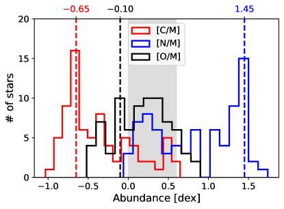
Figure 1: Distribution of measured elemental abundances from individual spectroscopy of 77 bright members of $\omega$ Centauri from Marino et al. (2012). The vertical dashed lines represent the values adopted in this study for the nominal population as per Table 1. The shaded area represents the range of oxygen abundances considered in secondary populations as per Table 2.

For every population, two sets of elemental abundances must be chosen: one for the zero age pre-main-sequence star (PMS) which will be used in evolutionary interior models; and one for the corresponding grid of model atmospheres. Ideally, the latter set must be informed by the final stages of fully evolved stars calculated using the former set. Unfortunately, this approach is not compatible with our method, in which the grid of model atmospheres is computed before the evolutionary models, necessitating an approximate treatment. With the exception of lithium, we assumed that the final atmospheric abundances match the initial PMS abundances, since any changes in composition induced by core nuclear fusion are expected to be insignificant at low masses, while models of higher mass ($\gtrsim 0.3\ \mathrm{M}_{\odot}$) develop interior radiative zones that preserve PMS abundances in the outer layers. Our calculated evolutionary models (to be described below) affirm this choice, with changes in abundances other than $\mathrm{Li}$ between the PMS and the surface of the fully evolved star never exceeding $\sim 0.1\ \mathrm{dex}$. On the other hand, the variation in lithium abundance in both the core and the atmosphere is significant, as shown in Figure 2. Atmospheric lithium is almost entirely consumed through proton capture for all but the smallest mass (insufficient central temperature for $\mathrm{Li}$ fusion) and the largest mass (formation of a radiative zone) models. Due to the minimal effect of lithium abundance on the stellar spectrum (and, even more so, synthetic photometry), we chose to ignore the minority of masses where $\mathrm{Li}$ is not depleted and assumed an abundance of $\mathrm{[Li/M]}=-3.0$ for all model atmospheres (but not for PMS in evolutionary models). This choice effectively eliminates lithium from the spectra.

The overall metallicity of the nominal population was chosen following Milone et al. (2017), who fit model isochrones onto $\omega$ Centauri photometry acquired with the HST Wide Field Channel of the Advanced Camera for Surveys (ACS/WFC) (Ryon, 2019) and the Infra Red channel of the Wide Field Camera 3 (WFC3/IR) (Dressel, 2012). While the isochrones in Milone et al. (2017) do not account for non-solar CNO abundances, they were consistent with observations and thus provide satisfactory starting parameters. Of the stellar populations identified in Milone et al. (2017), we specifically focused on the metal-poor side ($[\rm{Fe}/\rm{H}]\approx[\rm{M}/\rm{H}]\gtrapprox-1.7$) of the helium-rich ($\rm{Y}\approx 0.4$) MS-II population that corresponds to the blue sequence in Bedin et al. (2004). We set the lowest metallicity in the quoted range of MS-II as the initial guess for the nominal population, and allowed it to increase up to $[\rm{M}/\rm{H}]=-1.4$ in the secondary populations. We fixed the helium mass fraction to $\textrm{Y}=0.4$ for both nominal and secondary populations in accordance with both King et al. (2012) and Milone et al. (2017).

Milone et al. (2017) chose an isochrone age of $13.5\ \rm{Gyr}$, which we used in this investigation as well. The exact age of the cluster has little effect on the Main Sequence, which justifies using a single upper limit for the isochrone fitting regardless of the known variation in ages of individual members by a few $\rm{Gyr}$ (Marino et al., 2012). In contrast, brown dwarfs continuously evolve across colour-magnitude space, so our predictions were calculated for both $10\ \rm{Gyr}$ and $13.5\ \rm{Gyr}$ (Section 6).

Due to the multitude of populations in $\omega$ Centauri and the inevitable bias in abundances inferred by individual stellar spectroscopy, we perturbed the aforementioned parameters to generate $5$ sets of models for secondary populations, whose abundances are listed in Table 2. The perturbations were applied iteratively until the best fit to the observed population was achieved (see Section 5). All properties that are not mentioned in the table are identical to the nominal population.

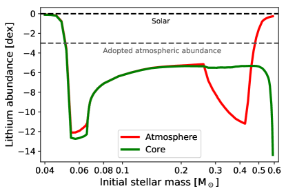
Figure 2: Depletion of lithium in the core and the atmosphere as a function of stellar mass for the HMMA secondary population (see Table 2) over $13.5\ \mathrm{Gyr}$. All models are initialized with a solar lithium abundance (see Appendix B) in the PMS phase. Atmospheric lithium is not depleted at $M\lessapprox 0.055\ \mathrm{M}_{\odot}$ due to insufficiently high temperatures for fusion, and at $M\gtrapprox 0.5\ \mathrm{M}_{\odot}$ due to the early formation of a radiative zone that “freezes” the surface abundance. At intermediate masses, lithium is depleted by proton capture in the core which is propagated into the atmosphere via convective mixing. At masses above $\approx 0.07\ \mathrm{M}_{\odot}$, trace amounts of lithium are also produced by incomplete proton-proton chains. For masses below $\approx 0.3\ \mathrm{M}_{\odot}$ no radiative zone exists and lithium abundances are nearly equally depleted throughout the star. A radiative zone forms between $0.3\ \mathrm{M}_{\odot}$ and $0.4\ \mathrm{M}_{\odot}$, where the atmospheric abundance first decreases compared to core due to late formation of the radiative zone and then increases due to early formation. A late radiative zone allows lithium depletion by proton capture to propagate into the envelope but prevents diffusion of lithium enhancement from the proton-proton chain.

$2$ Population $[\mathrm{O/M}]$ $[\alpha\mathrm{/M}]$ $[\mathrm{M/H}]$ LMHO (Low Metal High Oxygen) $0.6$ $0.0$ $-1.7$ HMET (High METal) $0.0$ $0.0$ $-1.4$ HMMO (High Metal Medium Oxygen) $0.4$ $0.0$ $-1.4$ HMMA (High Metal Medium Alpha) $0.0$ $0.4$ $-1.4$ HMHA (High Metal High Alpha) $0.0$ $0.6$ $-1.4$

Table 2: Properties of secondary populations

$3$ Ref Molecules # of lines (1) $\mathrm{H}\mathrm{O}\mathrm{D}$ $41.3\times 10^{6}$ (2) $\mathrm{H}_{2}\mathrm{O}$ $505\times 10^{6}$ (3) $\mathrm{CC}$, $\mathrm{CN}$, $\mathrm{CH}$, $\mathrm{NH}$, $\mathrm{OH}$, $\mathrm{SiO}$, $\mathrm{SiH}$, $\mathrm{H}_{2}$ $5.7\times 10^{6}$ (4) $\mathrm{CO}_{2}$ $4\times 10^{6}$ (5) $\mathrm{NH}_{3}$ $6.7\times 10^{3}$ (6) $\mathrm{ZrO}$, $\mathrm{YO}$ $267\times 10^{3}$ (7) $\mathrm{CO}$ $134\times 10^{3}$ (8) $\mathrm{C}_{2}\mathrm{H}_{2}$, $\mathrm{C}_{2}\mathrm{H}_{4}$, $\mathrm{C}_{2}\mathrm{H}_{6}$, $\mathrm{COF}_{2}$, $\mathrm{CH}_{3}\mathrm{OH}$, $\mathrm{CH}_{3}\mathrm{D}$, $\mathrm{N}_{2}$, $\mathrm{N}_{2}\mathrm{O}$, $\mathrm{NO}$, $\mathrm{NO}_{2}$, $\mathrm{NH}_{3}$, $\mathrm{OCS}$, $\mathrm{O}_{2}$, $\mathrm{O}_{3}$, $\mathrm{SO}_{2}$, $\mathrm{SF}_{6}$, $\mathrm{HI}$, $\mathrm{HCN}$, $\mathrm{HCOOH}$, $\mathrm{HNO}_{3}$, $\mathrm{HOCl}$, $\mathrm{HOBr}$, $\mathrm{HO}_{2}$, $\mathrm{HOD}$, $\mathrm{HF}$, $\mathrm{HCl}$, $\mathrm{HBr}$, $\mathrm{H}_{2}\mathrm{CO}$, $\mathrm{H}_{2}\mathrm{O}_{2}$, $\mathrm{H}_{2}\mathrm{O}$, $\mathrm{H}_{2}\mathrm{S}$ $1.3\times 10^{6}$ (9) $\mathrm{CO}_{2}$, $\mathrm{OH}$, $\mathrm{PH}_{3}$ $31.2\times 10^{3}$ (10) $\mathrm{CN}$ $2.2\times 10^{6}$ (11) $\mathrm{CH}_{4}$ $34.6\times 10^{3}$ (12) $\mathrm{H}_{3}^{+}$ $3.1\times 10^{6}$ (13) $\mathrm{CrH}$, $\mathrm{FeH}$, $\mathrm{TiH}$ $301\times 10^{3}$ (14) $\mathrm{MgH}$ $53.8\times 10^{3}$ (15) $\mathrm{CaH}$, $\mathrm{TiH}$, $\mathrm{VO}$ $14.6\times 10^{6}$ (16) $\mathrm{CH}_{4}$ $31.3\times 10^{6}$

Table 3: Molecular lines included in our PHOENIX setup

Note. — (1) – AMES water (Partridge & Schwenke, 1997), (2) BT water (Barber et al., 2006), (3) – Kurucz CD-ROM #15 (Kurucz, 1995), (4) – CDSD (Carbon Dioxide Spectroscopic Databank) (Tashkun & Perevalov, 2011), (5) – Sharp & Burrows (2007), (6) – Ferguson et al. (2005), (7) – Goorvitch (1994), (8) – HITRAN2004 (Rothman et al., 2005), (9) – HITRAN2008 (Rothman et al., 2009), (10) – Jorgensen & Larsson (1990), (11) – Brown (2005), (12) – Neale & Tennyson (1995), (13) – MoLLIST (Bernath, 2020), (14) – Weck et al. (2003), (15) – lines inherited from MARCS atmospheres (Plez, 2008), (16) – methane lines generated using STDS (Spherical Top Data System; Wenger & Champion 1998) in Homeier et al. (2003).

3.2 Model atmospheres

We calculate all model atmospheres with $T_{\mathrm{eff}}\leq 4000\ \mathrm{K}$ using a custom setup based on a branch of version 15.5 of the PHOENIX code (Hauschildt et al., 1997). Molecular lines considered in the calculation are listed in Table 3. Our modelling framework includes the formation of condensate clouds in the atmosphere and their depletion by gravitational settling according to the Allard & Homeier cloud formation model (Allard et al., 2012; Helling et al., 2008). At $T_{\mathrm{eff}}<3000\ \mathrm{K}$ we used the “cloudy” mode described in Gerasimov et al. (2020). For optimization purposes, a slightly simplified “dusty” mode is used at $T_{\mathrm{eff}}\geq 3000\ \mathrm{K}$, which differs in its coarser stratification ($128$ spherically symmetric layers instead of $250$), disabled gravitational settling, and fewer spectral features included in the calculation. It was verified that the transition between the two modes does not introduce noticeable discontinuities in the derived bolometric corrections and the difference between “cloudy” and “dusty” spectra at the transition temperature is insignificant. All PHOENIX models were calculated at wavelengths from $1\ \mbox{\AA}$ to $1\ \mathrm{mm}$ with a median resolution of $\lambda/\Delta\lambda\approx 18250$ in the range $$0.4\text{\,}\mathrm{\SIUnitSymbolMicro m}$\leq\lambda\leq$2.6\text{\,}\mathrm{\SIUnitSymbolMicro m}$$ and a lower resolution of $\sim 8000$ elsewhere.

At $T_{\mathrm{eff}}>4000\ \mathrm{K}$, the effects of both condensates and molecular opacities become subdominant, allowing us to replace PHOENIX with the much faster and simpler ATLAS code version 9 (Kurucz, 1970; Sbordone et al., 2004; Kurucz, 2014; Castelli, 2005). As opposed to PHOENIX, our ATLAS setup stratifies the atmosphere into $72$ plane-parallel layers covering the range of optical depths from $\tau=100$ to $\tau\sim 10^{-7}$. Instead of direct opacity sampling, ATLAS relies on pre-computed opacity distribution functions (ODFs) (Carbon, 1984). Convection is modelled using mixing-length theory (Böhm-Vitense, 1958; Smalley, 2005) with no overshoot. Modelled line opacities include $\sim 43\times 10^{6}$ atomic transitions of various ionization stages and $\sim 123\times 10^{6}$ molecular transitions including titanium oxide lines from Schwenke (1998) and water lines from Partridge & Schwenke (1997). We use satellite utilities DFSYNTHE and SYNTHE shipped with the main ATLAS code to compute a custom set of ODFs for the abundances of interest (one set for each considered population) and derive high-resolution synthetic spectra from the calculated models respectively. The calculated ODFs account for flux from $\sim 10\ \mathrm{nm}$ to $160\text{\,}\mathrm{\SIUnitSymbolMicro m}$ to ensure correct evaluation of energy equilibrium through the atmosphere. On the other hand, our synthetic spectra span a narrower range of wavelengths from $0.1\text{\,}\mathrm{\SIUnitSymbolMicro m}$ to $4.2\text{\,}\mathrm{\SIUnitSymbolMicro m}$, accommodating all instrument bands considered in this study. All SYNTHE spectra are calculated at the resolution of $\lambda/\Delta\lambda=6\times 10^{5}$.

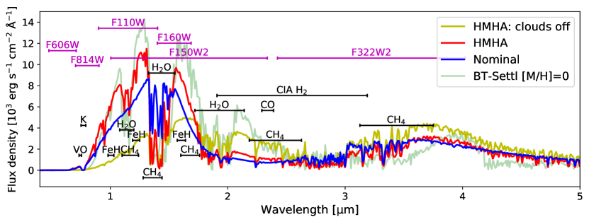
Figure 3: Synthetic spectra of selected low-temperature model atmospheres calculated in this study. Shown here are the $T_{\mathrm{eff}}=1200$, $\log_{10}(g)=5.0$ atmospheres from the nominal population (Table 1) and the HMHA population (Table 2). Both spectra demonstrate prominent molecular features, some of which are indicated with black bars (CIA $\mathrm{H}_{2}$ represents the band of collision-induced absorption by molecular hydrogen). A HMHA spectrum with identical parameters but calculated in the “dusty” mode (no gravitational settling) is shown for comparison. The corresponding synthetic spectrum for a model of solar metallicity from the BT-Settl library is also shown. Magenta bars delineate $20\%$ transmission bounds of HST ACS/WFC F814W and F606W bands; HST WFC3/IR F110W and F160W bands; and JWST NIRCam F150W2 and F322W2 bands. For clarity, the spectra are shown after convolution with a $3\ \mathrm{nm}$-wide Gaussian kernel.

A few examples of calculated low-temperature models are plotted in Figure 3. Compared to their solar metallicity counterparts, the spectra of metal-poor brown dwarfs are characterized by weaker molecular absorption (e.g., $3.5\text{\,}\mathrm{\SIUnitSymbolMicro m}$ methane band), more prominent collision-induced $\mathrm{H}_{2}$ absorption originating from deeper layers of the atmosphere, and extreme pressure broadening of alkali metal lines (e.g., K I resonant line at $0.77\text{\,}\mathrm{\SIUnitSymbolMicro m}$). Synthetic spectra computed under our setup have previously demonstrated good correspondence with observations of candidate metal-poor brown dwarfs in the field (Schneider et al., 2020). All calculated model atmospheres are publicly available in our online repository.

A typical PHOENIX model in the “cloudy” mode requires $\sim 150$ CPU hours to converge on the Comet cluster at the San Diego Supercomputer Center made available to us through the XSEDE programme (Towns et al., 2014). “Dusty” models were a factor of two or three faster to compute, while ATLAS models only took approximately $1$ CPU hour each.

3.3 Atmosphere-interior coupling

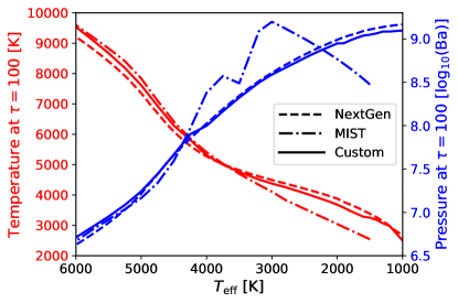
Figure 4: Comparison of three different sets of atmosphere-interior coupling boundary condition tables considered in this study at the surface gravity of $\log_{10}(g)=6.0$ and metallicity of $\mathrm{[M/H]}=-1.7$. NextGen (dashed line) refers to the PHOENIX grid from Allard et al. (2000); Hauschildt et al. (1999) that excludes gravitational settling in the atmosphere as well as enhancements of individual elements. MIST (dash-dotted line) refers to the ATLAS-derived tables used in Choi et al. (2016). The “custom” coupling (solid line) is based on newly calculated PHOENIX models at low $T_{\mathrm{eff}}$ and ATLAS models at high $T_{\mathrm{eff}}$ and includes individual elemental enhancements of the nominal population (Table 1) in addition to the metallicity scaling as described in text. Pressure is shown in CGS units of barye ($1\ \mathrm{Ba}=1\ \mathrm{dyn}\ \mathrm{cm}^{-2}$).

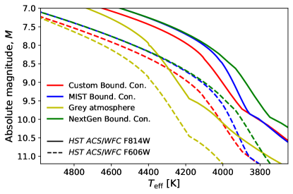
Figure 5: Effect of the choice of approach to atmosphere-interior coupling on synthetic photometry. The curves represent expected absolute magnitudes of the nominal population (see Table 1) as a function of effective temperature in two of the HST ACS/WFC bands: F814W (solid lines) and F606W (dashed lines), without interstellar extinction. The coupling schemes with pre-tabulated boundary conditions (Bound. Con.) are identical to those in Figure 4. The grey atmosphere coupling scheme at $\tau=2/3$ is shown for comparison, which is the default scheme in MESA.

We used the MESA code (Modules for Experiments in Stellar Astrophysics; Paxton et al. 2011) for all evolutionary calculations. At zero age, a MESA model is spawned as a PMS with a given total mass and uniform elemental abundances. The initial structure is determined by assuming a fixed central temperature well below the nuclear burning limit (in our case, $5\times 10^{5}\ \rm{K}$; Choi et al. 2016) and searching for a solution to the structure equations that reproduces the desired mass of the star. From here, evolution proceeds in dynamically determined time steps until the age of the model reaches the target age. On each step, the structure equations are solved using the atmospheric temperature and pressure as boundary conditions. Both can in principle be estimated from the current surface gravity and effective temperature of the model using an appropriate model atmosphere. It is those boundary conditions that establish the coupling between interiors and atmospheres. Once the interior structure of the star is known, the model can be advanced to the next time step by compounding expected changes due to diffusion, gravitational settling, nuclear reactions, mechanical expansion, and other time-dependent processes.

Our MESA configuration is derived from Choi et al. (2016) with a number of key differences outlined in detail in Appendix A. When handling atmosphere-interior coupling, MESA is able to estimate boundary conditions either by drawing them from a pre-computed table at a given optical depth or at run time using one of a variety of methods relying on simplifying assumptions such as grey atmosphere. The latter option is unlikely to be accurate at low effective temperatures where molecular opacities and clouds dominate the spectrum. The low-mass MESA setup employed by Choi et al. (2016) relies on boundary condition tables calculated at $\tau=100$ for a wide range of effective temperatures, surface gravities and metallicities. However, the accuracy of the tables at $T_{\mathrm{eff}}\lessapprox 3500\ \mathrm{K}$ is questionable, as they were derived from ATLAS atmospheres that fail to account for significant low-temperature effects such as condensation and molecular features.

In this study, we compared four different approaches to atmosphere-interior coupling:

• Run time calculation assuming grey atmosphere and drawing temperature and pressure at $\tau=2/3$;

• $\tau=100$ tables from Choi et al. (2016) at the $\omega$ Centauri metallicity, but not accounting for individual elemental enhancements or low-temperature atmospheric effects absent in ATLAS atmospheres;

• Custom $\tau=100$ tables drawn from NextGen, a publicly available PHOENIX grid (Allard et al., 2000; Hauschildt et al., 1999) without condensates or gravitational settling. The grid covers the $\omega$ Centauri metallicity, but not the individual elemental enhancements; and

• Custom $\tau=100$ tables drawn from our own atmosphere grids described above based on ATLAS at high temperatures and PHOENIX at low temperatures, including condensation and gravitational settling. The grids include all individual elemental enhancements for each of the considered populations.

The grids of model atmospheres calculated in this study span surface gravities from $\log_{10}(g)=4$ to $\log_{10}(g)=6$. At early ages ($\lesssim 2\ \mathrm{Myr}$), stars and brown dwarfs may briefly experience surface gravities under $\log_{10}(g)=4$, falling outside of the calculated atmosphere grid. In such instances, the boundary conditions from Choi et al. (2016) were used instead. By applying random perturbations to those low-gravity boundary conditions, we established that their accuracy has a negligible effect on the final results.

The temperature and pressure at $\tau=100$ for the tabular options are plotted as functions of effective temperature in Figure 4 at $\log_{10}(g)=6.0$. The effect of the chosen boundary conditions on synthetic photometry (described below) is shown in Figure 5. Both figures demonstrate good agreement between approaches at high effective temperatures, and increasing deviation at lower temperatures where atmosphere-interior coupling becomes important. The final set of interior models in our analysis use custom $\tau=100$ tables based on our own model atmospheres, which we believe to offer the highest accuracy. The comparison of different sets of boundary conditions is presented here to emphasize the importance of atmosphere-interior coupling and to demonstrate how significant changes in metallicity and elemental enhancements could be “mimicked” by inaccurate boundary conditions.

3.4 Synthetic photometry

Synthetic photometry of each modelled population of $\omega$ Centauri was computed by first evaluating the bolometric corrections of each bandpass of interest for each of the calculated model atmospheres. The bolometric correction is defined as

$$\mathrm{BC}_{x}=M_{b}-M_{x}=M_{b}+2.5\log_{10}\left(\frac{F_{x}}{F_{x}^{\prime}}\right)$$ (1)

where $x$ is a given bandpass; $\mathrm{BC}_{x}$ is the bolometric correction for $x$ between the absolute bolometric magnitude $M_{b}$ and the absolute magnitude in band $x$, $M_{x}$; $F_{x}$ is the total flux of the model through bandpass $x$; and $F_{x}^{\prime}$ is the total flux of the reference object through bandpass $x$. We used the VEGAMAG system for all comparisons to HST data and the ABMAG system for JWST predictions. For VEGAMAG, we used the apparent spectrum of Vega in Bohlin & Gilliland (2004) as our reference. For ABMAG, the reference spectrum is defined to be a constant flux density per unit frequency of $\approx 3631\ \mathrm{Jy}$ at all frequencies (Oke & Gunn, 1983). Both $F_{x}$ and $F_{x}^{\prime}$ are measured in photons per unit time per unit area (Bohlin et al., 2014) since all instruments of interest are photon-counting. $F_{x}$ (but not $F_{x}^{\prime}$) is taken at the distance of $10\ \mathrm{pc}$. By introducing the stellar radius $R$ we can express $F_{x}$ in terms of surface flux, $\Phi_{x}$:

$$\mathrm{BC}_{x}=M_{b}+2.5\log_{10}\left(\frac{\Phi_{x}}{F_{x}^{\prime}}\right)+5\log_{10}\left(\frac{R}{10\ \mathrm{pc}}\right)$$ (2)

Both $R$ and $M_{b}$ are dependent on the total luminosity of the model, $L$, which cannot be inferred from the model atmosphere on its own. For our purposes, $\mathrm{BC}_{x}$ must be re-expressed in terms of exclusively atmospheric parameters. The IAU definition of absolute bolometric magnitude (Mamajek et al., 2015) is

$$M_{b}=-2.5\log_{10}(L/[1\ \mathrm{W}])+\Delta$$ (3)

with $\Delta=71.197425$. Substituting in equation (2):

$$\mathrm{BC}_{x}=2.5\log_{10}\left(\frac{\Phi_{x}}{F_{x}^{\prime}}\right)-10\log_{10}\left(\frac{T_{\mathrm{eff}}}{1000~{}K}\right)+C$$ (4)

where $C=-30.88138$ is a constant evaluated as

$$C=\Delta-2.5\log_{10}\left[\frac{4\pi\sigma(10\ \mathrm{pc})^{2}(1000\ \mathrm{K})^{4}}{1\ \mathrm{W}}\right]$$ (5)

with $\sigma$ representing the Stefan-Boltzmann constant.

Finally, we rewrite the flux ratio, $\Phi_{x}/F_{x}^{\prime}$, in terms of the synthetic energy spectrum $\phi_{\lambda}$, reference energy spectrum $f^{\prime}_{\lambda}$ and the dimensionless transmission profile of $x$: $x_{\lambda}$:

$$\frac{\Phi_{x}}{F_{x}^{\prime}}=\frac{\int_{0}^{\infty}\lambda\phi_{\lambda}x_{\lambda}10^{-\frac{A_{\lambda}}{2.5}}d\lambda}{\int_{0}^{\infty}\lambda f_{\lambda}^{\prime}x_{\lambda}d\lambda}$$ (6)

In the case of ABMAG magnitudes, $f^{\prime}_{\lambda}$ must be converted from constant flux density per unit frequency as

$${f^{\prime}_{\lambda}}^{(\mathrm{ABMAG})}=(3631\ \mathrm{Jy})\frac{c}{\lambda^{2}}$$ (7)

where $c$ is the speed of light. Note that both integrands in equation (6) are multiplied by $\lambda$ to express the spectra in photon counts rather than units of energy. We have also introduced $A_{\lambda}$ – the extinction law in units of magnitude as a function of wavelength $\lambda$. We used the extinction law from Fitzpatrick & Massa (2007) parameterized by the optical interstellar reddening, $E(B-V)$, and the total-to-selective extinction ratio, $R_{V}=A_{V}/E(B-V)$. We assumed $R_{V}=3.1$ throughout and allowed $E(B-V)$ to be a free parameter, as described in Section 5.

For each of the modelled populations, a synthetic colour-magnitude diagram was constructed by calculating a grid of interior models with initial masses spanning from the lowest mass covered by the calculated model atmospheres ($0.03\ \mathrm{M}_{\odot}$ for the best-fit isochrone) to the highest mass compatible with our atmosphere-interior coupling scheme ($\sim 0.5\ \mathrm{M}_{\odot}$). At higher masses, $\tau=100$ lies too deep in the atmosphere, requiring a change in the reference optical depth (Choi et al., 2016) and potentially causing a numerical discontinuity in the calculated results. Since the upper mass limit of $0.5\ \mathrm{M}_{\odot}$ is sufficient to accommodate the vast majority of the available HST photometry (see Section 5), we chose to restrict our analysis to this upper mass limit, thereby avoiding the complexities of using multiple atmosphere-interior coupling schemes.

The bolometric corrections in the bands of interest were calculated as described above for each model atmosphere in the grid. Due to convergence issues associated with cloud formation at very low effective temperatures, a few models with maximum flux errors in radiative zones exceeding $10\%$ were excluded from the atmosphere model grid. The remaining grid was then interpolated in effective temperature and surface gravity to the final surface parameters of each evolutionary interior model at the target age. Finally, the interpolated bolometric corrections were combined with the bolometric magnitudes of each interior model to obtain the desired synthetic photometry.

3.5 Results

Figure 6 shows the calculated isochrone of the nominal population of $\omega$ Centauri as defined in Table 1. The isochrone is plotted in the absolute pre-extinction colour-magnitude spaces defined by the HST ACS/WFC F606W and F814W optical bands and the HST WFC3/IR F110W and F160W near infrared bands. The isochrone displays a characteristic inflection point around $\sim 0.3\ \mathrm{M}_{\odot}$ due to the change in the adiabatic gradient induced by the formation of molecules in the envelope (Copeland et al., 1970; Calamida et al., 2015; Pulone et al., 2003; Cassisi, 2011). This feature is particularly valuable in our fitting process (Section 5) due to its sensitivity to chemical abundances and dense coverage by our observations. The near infrared isochrone shows a prominent Main Sequence knee at $\sim 0.1\ \mathrm{M}_{\odot}$ where the flux in F160W is suppressed by the onset of $\mathrm{H}_{2}$ collision-induced absorption (Linsky, 1969; Saumon et al., 1994; Saracino et al., 2018), resulting in bluer colours at lower masses. This overall shift of peak emission towards shorter wavelengths has been spectroscopically observed in L and T subdwarfs (Burgasser et al., 2003; Schneider et al., 2020). The hydrogen-burning limit (HBL) encompasses another reversal of the colour-magnitude slope in both diagrams at a mass of $\sim 0.07\ \mathrm{M}_{\odot}$ (detailed calculation in Section 6 yields $\mathrm{M}_{\mathrm{HBL}}$ = $0.069\ \mathrm{M}_{\odot}$). As the stellar mass decreases past the limit, the population cools rapidly into the brown dwarf regime. At optical wavelengths, brown dwarfs of lower masses appear marginally bluer immediately after the HBL due to the pressure-broadened K I line absorption centered at $0.77$ $\micron$ and extending across in the F814W band (Allard et al., 2007, 2016).

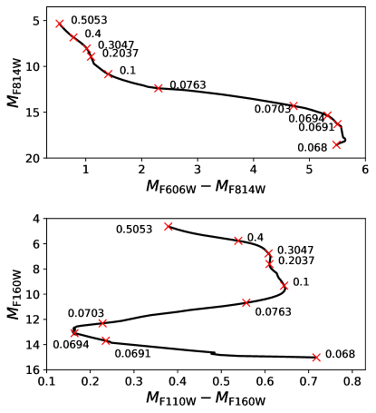
Figure 6: Isochrones derived for the nominal population of $\omega$ Centauri in optical (top) and near infrared (bottom) absolute colour-magnitude spaces. The optical isochrone is evaluated for HST ACS/WFC filters, while the near infrared isochrone is evaluated for HST WFC3/IR filters. Red markers display the initial stellar masses of selected models along the isochrone in units of solar masses. Extinction effects are not included.

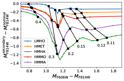
Figure 7: Isochrones for secondary populations listed in Table 2. Absolute magnitudes (vertical axis) are displayed as differences after subtracting the absolute magnitude of the nominal population in Fig 6 at the corresponding colour. The range of colours displayed matches the range covered by the available HST data, even though some of the isochrones have been calculated at much redder colours. Black lines join the points of equal initial masses along the isochrones that are labeled in solar masses. Extinction effects not included. All magnitudes correspond to HST ACS/WFC filters.

The behavior of secondary populations around the $0.3\ \mathrm{M}_{\odot}$ inflection is shown in Figure 7 as differences to the nominal isochrone in absolute F814W magnitude. In general, all secondary populations are brighter than the nominal one at identical colours, redder at identical masses, and display a more prominent variation in slope. The effect becomes more apparent at higher metallicities and $\alpha$-enhancements, but shows little dependence on the oxygen enhancement alone, suggesting that the lack of a well-defined oxygen peak in Figure 1 is not expected to pose difficulties to isochrone fitting.

4 Observations

To determine the best-fit isochrone for $\omega$ Centauri, we compared each population isochrone to photometric data acquired with HST ACS/WFC in the F606W and F814W bands (programmes GO-9444 and GO-10101; PI: King), and HST WFC3/IR in the F110W and F160W bands (programmes GO-14118 and GO-14662 for WFC3; PI: Bedin). Observations were carried out in a $3^{\prime}\times 3^{\prime}$ field situated $\sim 3$ half-light radii ($\approx 7^{\prime}$) southwest of the cluster centre (see field F1 in Figure 1a of Bellini et al. 2018). This is the deepest observed field for $\omega$ Centauri for which both optical and near infrared HST observations are available.

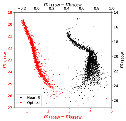
Figure 8: Proper motion-selected zero-pointed differential reddening-corrected photometry of the Main Sequence of $\omega$ Centauri. Optical photometry was acquired with HST ACS/WFC and near infrared photometry with HST WFC3/IR. Only unsaturated stars are shown for the optical photometry. The Main Sequence bifurcation can be seen in both datasets.

The primary data reduction followed the procedure described in Scalco et al. (2021) for two other HST $\omega$ Centauri fields, and is analogous to methods adopted in numerous previous works (Bellini et al., 2017a, 2018; Milone et al., 2017; Libralato et al., 2018; Bedin et al., 2019). In brief, positions, fluxes and multiple diagnostic quality parameters were extracted using the point spread function (PSF) fitting software package KS2 (Anderson & King, 2006; Anderson et al., 2008); see Scalco et al. (2021) and references therein. The photometric zero-point onto the VEGAMAG system was determined using the approach of Bedin et al. (2005). The sample was filtered by quality parameters $\sigma$ (photometric error), QFIT (correlation between pixel values and model PSF), and RADXS (flux outside the core in excess of PSF prediction; Bellini et al. 2017a; Bedin et al. 2008), as described in Scalco et al. (2021, Section 4).

We used the relative proper motions of sources in the observed region to separate field stars from cluster members. Proper motions were obtained by comparing the extracted positions of stars measured in the earliest and latest programmes (GO-9444 and GO-14662, respectively), providing epoch baselines of up to $15$ years. Photometry in each filter was corrected for systematic photometric offsets following Bedin et al. (2009). A general correction for differential reddening was also applied following the method described in Bellini et al. (2017b, Section 3).

Measurement of the LF (Section 5) requires quantification of source completeness as a function of colour and magnitude, for which we followed the approach described in Bedin et al. (2009). We generated a total of $2.5\times 10^{5}$ artificial stars (AS) with random positions. For each AS, a F606W magnitude was drawn from a uniform distribution. The remaining three magnitudes (F814W, F110W, F160W) were then chosen to place the AS along the approximate ridgeline of the Main Sequence in various colour-magnitude spaces. AS were introduced in each exposure and measured one at a time to avoid over-crowding, making the process independent of the LF. A star was considered recovered when the difference between the generated and measured star position was less than $0.1$ pixels and the magnitude difference was less than $0.4\ \mathrm{mag}$. Finally, the stars were divided into half-magnitude bins and the photometric errors and completeness for each bin were computed.

The near infrared and optical colour-magnitude diagrams based on our observations are shown in Figure 8. The full catalogue of source astrometry, photometry, membership, and completeness is provided as an associated data product and described more fully in Appendix C.

5 Evaluation

With mass-luminosity and colour-magnitude sequences computed for multiple populations, we were able to determine the optimal isochrone and IMF by comparing the predictions of those models to the HST-observed Main Sequence at optical and near infrared wavelengths.

5.1 Best-fit isochrone

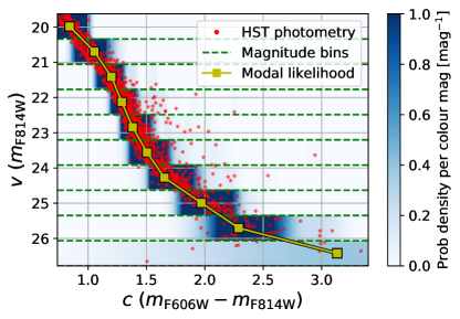
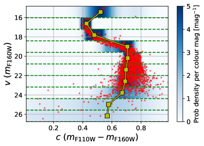
Figure 9: Colour probability distributions inferred from the observed scatter in HST photometry. Also shown are the boundaries of the magnitude bins used in our fitting analysis. Yellow markers indicate the mode of the distribution in each bin. Top: Optical data from HST ACS/WFC. Bottom: Near infrared data from HST WFC3/IR.

We adopted a distance modulus of $13.60\pm 0.05$ based on the distance to $\omega$ Centauri of $5.24\pm 0.11\ \mathrm{kpc}$ derived by Soltis et al. (2021) from the parallaxes of $\sim 7\times 10^{4}$ members. The adopted value is marginally smaller than the distance modulus of $13.69$ derived by Cassisi et al. (2009) from isochrone fit to the CMD.

We sought an isochrone that is most statistically compatible with the observed photometry, accounting for the average spread in the data introduced by unmodelled astrophysical and instrumental phenomena, such as the variation in abundances across the cluster, multiple star systems, observational errors, etc. First, we developed a likelihood model that predicts the probability of finding a cluster member at a given point $(c,v)$ in colour-magnitude space assuming that the average population is well-described by one of our isochrones:

$$\begin{split}\mathcal{P}_{E}(c,v)\propto\int{\xi(m)P\left(c,v\Bigm{|}c_{0}(m,E),v_{0}(m,E)\right)dm}\end{split}$$ (8)

In the equation, $P(...)$ is the probability of observing a member at $(c,v)$ assuming that the “true” location of the star in the colour-magnitude space (including reddening) is $(c_{0},v_{0})$. Both $c_{0}$ and $v_{0}$ are functions of the initial stellar mass, $m$, and the optical interstellar reddening $E$. Finally, $\xi(m)$ is the IMF, such that $\xi(m)dm$ is the number of stars in the cluster with masses between $m$ and $m+dm$. Note that a proportionality sign is used here as the likelihood function is not appropriately normalized in the given form.

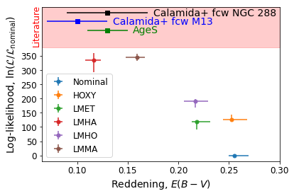
Figure 10: Likelihoods of compatibility and best-fit interstellar reddening for the population isochrones calculated in this study based on HST photometry. “Nominal” refers to the nominal population described in Section 3. Secondary populations are summarized in Table 2. The vertical axes are normalized to $\mathcal{L}_{\mathrm{nominal}}$. Error bars indicate random errors in the values as described in text. Selected reddening values from literature are also shown with their uncertainties. AgeS refers to the reddening estimate used in Thompson et al. (2001, green). The other two values are taken from Calamida et al. (2005), calculated from comparison with (fcw) NGC 288 (black) and M13 (blue). Marker shapes differentiate between fits obtained using optical ACS/WFC3 (squares; right axis) and near infrared WFC3/IR photometry (triangles; left axis). The two sets of values have different vertical scaling and cannot be compared against each other.

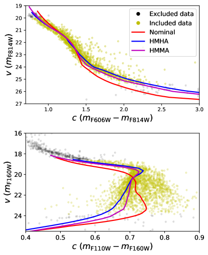
Figure 11: Nominal (Table 1) and two secondary (Table 2) population isochrones overplotted on HST photometry. The isochrones have been adjusted by the best-fit reddening values. The colour of markers indicates whether any particular member was or was not included in the log-likelihood optimization described in text to evaluate the accuracy of the isochrone. Top: Optical data from HST ACS/WFC. Bottom: Near infrared data from HST WFC3/IR.

The individual probability distribution, $P(...)$, encapsulates the scatter of photometry around the best-fit isochrone, and must account for all relevant effects including experimental uncertainties, unresolved multiple stars, and multiple distinct populations known to be present in $\omega$ Centauri. For our purposes, both $P(...)$ and $\xi(m)$ can be estimated empirically from the observed spread of HST data across the colour-magnitude space without theoretical input. In this method, the scatter along the colour axis is degenerate with that along the magnitude axis, as any observed distribution of data points may be reproduced by perturbing predicted photometry along only one axis and not the other. We therefore chose to sample the observed scatter in photometry along the colour axis only and use the magnitude axis as an estimator of the initial stellar mass by interpolating the theoretical mass-luminosity relation for the population under evaluation.

The empirical scatter was sampled from the observed data as follows. First, the range of apparent magnitudes in $v$ (F814 in the optical, F160W in the near infrared) was divided into $10$ bins of equal widths as demonstrated in Figure 9. Within each bin, the variation of magnitude was ignored and the probability density function (PDF) of the colour distribution was computed using Gaussian kernel density estimation with bandwidths calculated as in Scott (2015). The distribution was then translated along the colour axis to place the mode at the origin. The inferred PDF around the mode was then used as the scatter in colour for all stars whose magnitudes fall within the magnitude bin.

The initial mass function in equation (8), $\xi(m)$, was evaluated by converting all measured magnitudes in the HST dataset to initial stellar masses using the linearly interpolated mass-magnitude relations derived from stellar models discussed in Section 3. The inferred distribution of masses was then converted into the mass PDF, $\xi(m)$, using the same kernel density estimation method as in the colour spread (Scott, 2015), but trimmed on both sides at the lowest and highest modelled stellar masses respectively to avoid extrapolation.

The integral in equation (8) was computed numerically by drawing $10^{4}$ masses from the inferred $\xi(m)$ PDF, evaluating the integrand for each and summing the results. Finally, the total likelihood of a given isochrone being compatible with the HST dataset ($\mathcal{L}(E)$) was calculated as in equation (9).

$$\begin{split}\mathcal{L}(E)\propto\prod_{i}\mathcal{P}_{E}(c_{i},v_{i})\end{split}$$ (9)

In the equation, the product may, in principle, be taken over all individual measurements $(c_{i},v_{i})$. In practice, we must only include those members in the HST dataset that fall within the magnitude range of all calculated isochrones, as stellar masses of members out of range cannot be reliably estimated. Furthermore, since inferred stellar masses are dependent on interstellar reddening which is not a priori known, we must only select those cluster members for analysis that fall within the modelled range at all realistic reddenings, which we conservatively take to be $E(B-V)\in[0.0,0.4]$. Our final choice of bounds was $v\in(18.65,23.83)$ in the near infrared (WFC3/IR F160W) and $v\in(19.99,25.44)$ in the optical (ACS/WFC F814W), accommodating approximately $85\%$ and $94\%$ of all available measurements, respectively. The subset of selected members is shown in Figure 11.

For the nominal and each of the secondary populations, we maximize $\mathcal{L}(E)$ with respect to the interstellar reddening, $E(B-V)$. We estimate the random error in the best-fit reddening value, $E_{0}$ by considering three contributions. The intrinsic fitting error may be adopted as the Cramér–Rao bound:

$$\mathrm{Var}\left(E_{0}\right)=-\left(\frac{\delta^{2}\ln\mathcal{L}}{\delta E^{2}}\Bigm{|}_{E=E_{0}}\right)^{-1}$$ (10)

which in our case evaluated to $\sqrt{\mathrm{Var}\left(E_{0}\right)}\approx 0.001$ for all isochrones. The contributions of the random sampling of $\xi(m)$ during numerical integration and experimental uncertainties in the data were estimated by repeating the fitting process $10$ times with different samples of $\xi(m)$ and random Gaussian perturbations in the data. Finally, the error induced by the uncertainty in the distance to the cluster was determined by repeating the fitting process for upper and lower $1\sigma$ bounds on the distance modulus value.

All of the aforementioned contributions were combined in quadrature. The resulting likelihoods and best-fit reddening values are shown in Figure 10 with uncertainties. Every secondary isochrone performs better than the nominal one, with HMHA offering the best fit in both optical and near infrared wavelengths. As such, we used HMHA for our predictions of brown dwarf photometry described in Section 6. The best-fit reddening values corresponding to this isochrone are $E(B-V)=0.238\pm 0.003$ from the near infrared data and $E(B-V)=0.17\pm 0.01$ from the optical data. The random errors in both $E(B-V)$ estimates quoted here and shown in Figure 10 are likely not representative of the true uncertainty in the value, which is primarily driven by systematic effects due to the simplified population parameters, the reddening law, and errors intrinsic to the calculated stellar models. The scatter in $E(B-V)$ estimates between the optical and near infrared datasets suggests that the true value of the uncertainty in reddening is of the order of $\sim 0.07$.

Our reddening estimates exceed most literature values, of which three are shown in Figure 10. The Cluster AgeS experiment (Thompson et al., 2001) uses the value of $E(B-V)=0.13\pm 0.02$ based on the value of $E(B-V)=0.132$ given by the map of dust emission from Schlegel et al. (1998) at a particular point within $\omega$ Centauri and assuming the uncertainty of $0.02$ motivated by the variation of reddening across the cluster. In Calamida et al. (2005), two reddening values of $E(B-V)=0.13\pm 0.04$ and $E(B-V)=0.10\pm 0.03$ are derived from comparison with NGC 288 and M13, respectively. The apparent discrepancy in reddening values may be an artifact of our approach, since a single population is used to model both Main Sequences of the cluster. Consequently, the large helium fraction adopted in this study makes the predicted colours around the Main Sequence knee bluer, corresponding to a higher best-fit reddening value.

Two best-fitting secondary isochrones – HMHA and HMMA – as well as the nominal isochrone are plotted against the HST data in Figure 11, visually illustrating the goodness-of-fit. Both isochrones in the figure have been corrected for the corresponding best-fit interstellar reddening parameters.

5.2 Best-fit LF and IMF

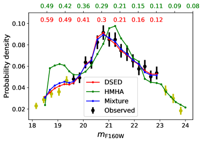
Figure 12: Observed luminosity function (LF) for $\omega$ Centauri (black) with three theoretical fits corresponding to the cases of $\mu=0$ (red, solar helium population only), $\mu=1$ (green, enhanced helium population only) and $\mu$ being a free parameter (both populations). The enhanced helium population is based on the mass-luminosity relation of the best-fit isochrone calculated in this study, HMHA. The solar helium population is based on the mass-luminosity relationship from Dotter et al. (2008, DSED). In each case, a broken power law IMF is assumed (Equation 11) with the best-fit values $\gamma=0.89\pm 0.06$, $\gamma=0.50\pm 0.07$ and $\gamma=0.83\pm 0.08$ for the three cases respectively. The best-fit mixing fraction in the case of two populations was calculated as $\mu=0.15\pm 0.14$. The fitting is carried out between the apparent magnitudes of $19.5$ and $23$ only since DSED models are not available at the faint end and photometry becomes increasingly unreliable at the bright end due to saturation (Scalco et al., 2021). Nonetheless, the observed LF outside this range is shown in yellow for completeness. The normalization on the vertical axis is such that the sum of all bins used in the fit is unity. The upper colour-coded horizontal axis indicates the initial stellar masses corresponding to magnitudes for the solar helium population (red) and the enhanced helium population (green) in solar masses.

Assuming the best-fit (HMHA) isochrone to be representative of the average distribution of $\omega$ Centauri members in colour-magnitude space, we now seek a suitable IMF for the cluster to estimate the population density. As will be demonstrated shortly, the cluster is well described by a broken power law:

$$\xi(m)\propto\begin{cases}m^{-2.3},&\text{if }m>0.5\ \mathrm{M}_{\odot}\\ m^{-\gamma},&\text{if }m\leq 0.5\ \mathrm{M}_{\odot}\\ \end{cases}$$ (11)

The power index of the high-mass regime ($-2.3$) as well as the breaking point ($m=0.5\ \mathrm{M}_{\odot}$) are fixed to the values employed in the “universal” IMF derived in Kroupa (2001). It has been demonstrated by Sollima et al. (2007) that those values are well-suited to the high-mass regime of $\omega$ Centauri. The power index of the low-mass regime ($-\gamma$) is allowed to vary. For comparison, Sollima et al. (2007) use $\gamma=0.8$, while the “universal” IMF introduces additional breaking points with different power indices.

The theoretical mass-luminosity relationship for HMHA was combined with the IMF to derive the theoretical luminosity function (LF) for $\omega$ Centauri as a function of $\gamma$. The best value of $\gamma$ was determined by optimizing the $\chi^{2}$ statistic for the goodness-of-fit between the theoretical and observed LFs. Our analysis of the LF was carried out in the F160W band of HST WFC3/IR between the apparent magnitudes of $19.5$ and $23$. Within this range, the data were divided into $15$ uniform bins with the count uncertainty in each bin taken as the square root of the count. The counts have also been adjusted for estimated sample completeness in each bin as discussed in Section 4. The histogram was normalized and used as an estimate of the underlying PDF.

The theoretical LF was calculated from the IMF in equation (11) using the mass-luminosity relationship from HMHA and integrating the resulting PDF within each magnitude bin. Both observed and theoretical LFs within the fitting range are plotted in Figure 12 in green and black respectively for the best-fit value of $\gamma=0.50\pm 0.07$. The correspondence between the two LFs appears poor, indicating that the HMHA population alone cannot reproduce the observed LF. This result is not surprising as our best-fit isochrone was calculated for the helium mass fraction of the blue sequence in $\omega$ Centauri that is only representative of a minority of the members.

To improve the fit, we added a second population with a solar helium mass fraction and a mass-luminosity relationship adopted from the Dartmouth Stellar Evolution Database (DSED; Dotter et al. 2008) for $[\mathrm{M}/\mathrm{H}]=-1.7$ and $\mathrm{Y}=0.2456$. The extinction of $0.085\ \mathrm{mag}$ was applied to synthetic F160W photometry from DSED based on the average magnitude difference between the best-fit reddening ($E(B-V)=0.17$, lower bound most consistent with literature) and reddening-free ($E(B-V)=0$) HMHA isochrones. The mixing fraction between the two populations, $\mu$, was treated as a free parameter varying between $0$ (DSED population only) and $1$ (HMHA only). The best-fit LF based on both HMHA and DSED as well as the best-fit based on DSED alone ($\mu=0$) are shown in Figure 12. The calculated best-fit value of $\mu=0.15$, is comparable to its uncertainty of $\pm 0.14$. Therefore, we present this result as the $2\sigma$ upper limit on the blue sequence population fraction, $\mu<0.45$. The blue sequence thus contributes less than $45\%$ of the cluster population in the observed region, in agreement with Bellini et al. (2009). The best-fit value of $\gamma$ when both HMHA and DSED LFs are included is $0.83\pm 0.08$, which matches the adopted value of $\gamma$ in Sollima et al. (2007).

6 Predictions

6.1 Substellar population of $\omega$ Centauri

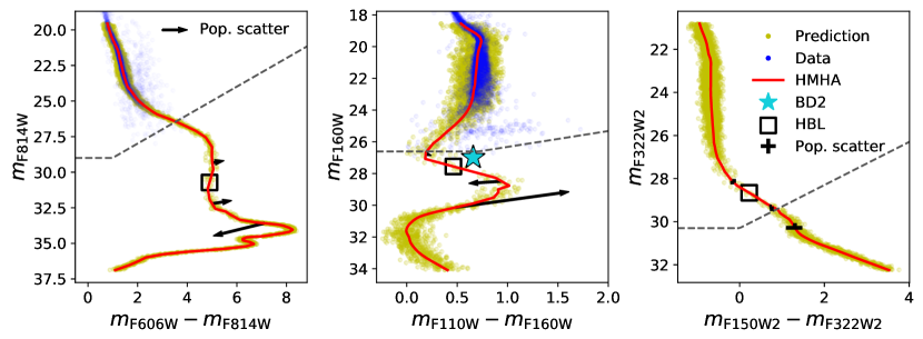
Figure 13: Predicted colour-magnitude diagrams for $\omega$ Centauri from the Main Sequence through the stellar/substellar gap and down to the appearance of first brown dwarfs. Predicted points are based on the best-fit HMHA isochrone and the best-fit IMF. For clarity, a Gaussian scatter in colour by $0.1$ magnitudes was added to each point. Where available, predicted CMDs are shown alongside existing HST photometry reaching the cool end of the Main Sequence. All CMDs are normalized to $1700$ objects between $0.1\ \mathrm{M}_{\odot}$ and $0.3\ \mathrm{M}_{\odot}$. The instruments used are HST ACS/WFC (left), HST WFC3/IR (middle) and JWST NIRCam (right). The cyan star shows the near infrared colour and magnitude of BD2 – a candidate brown dwarf in the globular cluster M4 from Dieball et al. (2019). The magnitude of BD2 shown here has been adjusted for the difference between the distance moduli of $\omega$ Centauri and M4 using the distance measurement from Neeley et al. (2015). The grey dashed line indicates the approximate faint limit for both HST datasets and the expected faint limit of future JWST measurements, calculated using the JWST Exposure Time Calculator (Pontoppidan et al., 2016) for a $1\ \mathrm{hr}$ exposure and signal-to-noise ratio of $2$. The colour and magnitude corresponding to the hydrogen-burning limit (HBL) are highlighted in each case. The arrows in the HST plots (left and middle) indicate the approximate direction and relative magnitude of the effect of decreasing metallicity and $\alpha$-enhancement as estimated from the difference between the best-fitting HMHA and HMMA secondary populations as well as the nominal population. In the case of JWST, the scatter among isochrones does not display a clear direction and is shown with error bars instead.

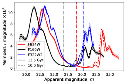
Figure 14: Predicted luminosity function for the HST ACS/WFC F814W band, the HST WFC3/IR F160W band, and the JWST NIRCam filter F322W2. Curves are shown for the population ages of $13.5\ \mathrm{Gyr}$ (solid) and $10\ \mathrm{Gyr}$ (dashed). The two peaks correspond to the Main Sequence and brown dwarfs in the cluster with a stellar/substellar gap in between. The vertical dash-dotted lines indicate the approximate faint limits for the instruments shown, calculated identically to Figure 13. The shaded areas around the curves indicate the range of our predictions based on the uncertainty in the determined IMF. While the shown ranges are for the age of $13.5\ \mathrm{Gyr}$, similar uncertainties apply to the case of $10\ \mathrm{Gyr}$. This figure demonstrates the superiority of infrared observations with JWST as the apparent magnitude of brown dwarfs enters the limit of the instrument.

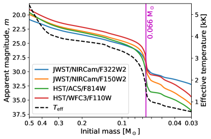
Figure 15: Predicted mass-luminosity relations for the same set of instruments as in Figure 14 as well as the predicted mass-effective temperature relationship (dashed). The approximate mass of the hydrogen-burning limit is highlighted with a vertical line and labelled.

In this section, we present our predictions of colours, magnitudes and CMD densities of brown dwarfs in $\omega$ Centauri using the best-fit isochrone (HMHA) and the best-fit IMF (Equation 11) calculated in Section 5. Figure 13 shows predicted CMDs for the cluster in three different sets of filters: F814W vs F606W-F814W for HST ACS/WFC, F160W vs F110W-F160W for HST WFC3/IR and F322W2 vs F150W2-F322W2 for JWST NIRCam.

For the first two diagrams, observed Main Sequence photometry is available and shown alongside predicted colours and magnitudes in blue. The density of points in the predicted set is proportional to the PDF luminosity function (Figure 12) extended into the brown dwarf regime. The normalization is such that approximately $1700$ points fall between the initial masses of $0.1\ \mathrm{M}_{\odot}$ and $0.3\ \mathrm{M}_{\odot}$. This choice closely matches the number of members within the same range of masses in the optical HST dataset used in this analysis. For clarity, a Gaussian spread with a standard deviation of $0.1$ magnitudes was applied to each point from the predicted set along the colour axis. Each CMD contains a region of low source density below the cool end of the Main Sequence (the stellar/substellar gap) followed by an increase in density at fainter magnitudes, corresponding to the accumulation of cooling brown dwarfs.

The effects of metallicity and $\alpha$-enhancement on the predicted brown dwarf colours and magnitudes are indicated by error bars and arrows in Figure 13 at three effective temperatures: $1900\ \mathrm{K}$, $1300\ \mathrm{K}$, and $1000\ \mathrm{K}$. The first temperature is just above the HBL, while and the latter two are below the HBL. The effect size was inferred from the scatter among the two best-fit isochrones, HMHA and HMMA, and the nominal isochrone. Note that at $T_{\mathrm{eff}}=1000\ \mathrm{K}$, only the best-fit isochrone (HMHA) has computed atmosphere models, so scatter at this temperature is based on extrapolated bolometric corrections for both HMMA and the nominal isochrones and may be unreliable. The scatter is substantial in the optical and near infrared HST bands, but appears far less significant in infrared JWST bands, as the F150W2 band accommodates most of the prominent metallicity features in the spectrum (see Figure 3). A different choice of narrow-band filters would make colour measurements more sensitive to chemical abundances at the expense of worse signal-to-noise ratio.

The extended luminosity functions that the CMD predictions are based on are shown in Figure 14. As before, both the main peak corresponding to the Main Sequence and the brown dwarf peak just emerging at the faint end can be seen with a gap in between. In the figure, each plot is given for two cluster ages of $10\ \mathrm{Gyr}$ and $13.5\ \mathrm{Gyr}$ corresponding to the expected ages of the youngest and oldest members in $\omega$ Centauri. While the Main Sequence peaks appear relatively unaffected by age, the brown dwarf peaks emerge at slightly brighter magnitudes at $10\ \mathrm{Gyr}$. As expected for objects in energy equilibrium, the Main Sequence evolves slowly with time. By contrast, substellar objects have entered their cooling curves and are moving steadily across colour-magnitude space. Hence, the luminosity function gap for $\omega$ Centauri and other globular clusters provides a potential age diagnostic for the system, assuming the evolutionary timescales are correctly modeled (Caiazzo et al., 2017, 2019; Burgasser, 2004, 2009). We also show in Figure 14 the variance in LF predictions taking into account uncertainty in the inferred IMF. In general, a higher value of the power index results in fewer low-mass members in the cluster and vice versa. Note that the width of the stellar/substellar gap is insensitive to the adopted IMF and is primarily determined by the mass-effective temperature relationship of the population. The normalization in Figure 14 is for the total number of helium-enriched members in the entire cluster based on the best-fit IMF (Equation 11), the best-fix mixing ratio ($\mu=0.15$) and the assumed total cluster mass of $4\times 10^{6}\ \mathrm{M}_{\odot}$ (D’Souza & Rix, 2013).

Finally, we provide a set of mass-luminosity relations for the aforementioned JWST and HST filters in Figure 15 alongside the mass-effective temperature relationship. All curves are based on the best-fit isochrone (HMHA). The predicted initial stellar mass at the hydrogen-burning limit (HBL) was taken as the mass for which the total proton-proton chain luminosity output corresponds to a half of the total luminosity output at $13.5\ \mathrm{Gyr}$. This limit was found to be $\mathrm{M}_{\mathrm{HBL}}$ = $0.066\ \mathrm{M}_{\odot}$ for HMHA (Figure 15). For comparison, the HBL for the nominal population is at a marginally higher value of $\mathrm{M}_{\mathrm{HBL}}$ = $0.069\ \mathrm{M}_{\odot}$. A higher HBL mass is expected for stars with lower metallicity as the corresponding reduction in atmospheric opacity results in faster cooling and requires a higher rate of nuclear burning (higher core temperature) to sustain thermal equilibrium. We note that the hydrogen-burning limits calculated here are lower than most literature estimates (e.g. Chabrier & Baraffe 1997) due to the increased helium mass fraction that stimulates faster hydrogen fusion in the core, allowing stars of lower masses to establish energy equilibrium.

6.2 Unresolved binary systems

A fraction of brown dwarfs in $\omega$ Centauri may be multiple systems which will appear brighter due to the superposition of fluxes from individual components. Existing constraints from the luminosity function (Elson et al., 1995) and the radial velocity distribution (Mayor et al., 1996) suggest that $\omega$ Centauri has an unusually low binary fraction of at most a few percent among hydrogen-burning members which is likely to be lower yet for the substellar population of the cluster (Burgasser et al., 2007; Fontanive et al., 2018). We may therefore safely ignore the effect of triple and higher-order systems that are far less likely to form than binary systems (Raghavan et al., 2010).

The effect of unresolved binary systems is determined by the binary fraction of the cluster as well as the distribution of the component mass ratio, $q=M_{s}/M_{p}$ where $M_{s}$ and $M_{p}$ are the masses of the secondary and primary components respectively and $q\leq 1$. To quantify the effect, we carried out numerical simulations where a number of randomly chosen objects in the JWST predicted dataset received secondary components with masses drawn according to the commonly used (Kouwenhoven et al., 2009) power law distribution of mass ratios, $P(q)\propto q^{\beta}$. In each case, the probability distribution was trimmed at the minimum value of $q$ that ensures the secondary mass remains within the mass range of the best-fit isochrone HMHA. We considered a range of $\beta$ values from $\beta=-0.5$ calculated by Reggiani & Meyer (2011) for a variety of star forming regions, to $\beta=4$ used by Burgasser et al. (2006) for field brown dwarfs. We found the companion mass distribution at the lowest value of $q$ to closely resemble that obtained through random pairing of cluster members for our IMF. On the other hand, the highest considered value of $\beta$ emphasizes preference for components with similar masses corresponding to the so-called “twin peaks” effect (Lucy & Ricco, 1979; Kouwenhoven et al., 2009).

We found that the width of the stellar/substellar gap shown in Fig. 14 is not noticeably affected by binary systems for binary fractions under $0.5$ due to the smooth rise in brown dwarf number density with magnitude. The average brightness of modelled brown dwarfs increased by $\sim 0.1\ \mathrm{mag}$ for the case of $\beta=4$ and a binary fraction of $0.2$. For the more realistic binary fraction of $0.05$, the magnitude difference did not exceed $0.03\ \mathrm{mag}$ for all considered values of $\beta$, falling well within the expected uncertainty of future $JWST$ measurements. We therefore conclude that magnitude predictions for brown dwarfs in $\omega$ Centauri presented in this work are not noticeably affected by any realistic population of unresolved multiple star systems in the cluster.

7 Conclusion

In this study, we calculated a new set of theoretical isochrones, mass-luminosity relations, and colour-magnitude diagrams for the helium-rich members of the globular cluster $\omega$ Centauri. Our predictions provide a theoretical expectation for the first observations of brown dwarfs in globular clusters anticipated with JWST. At present, globular cluster photometry extends below the faint end of the Main Sequence, but not deep enough to robustly sample the brown dwarf population. The predictions presented in this paper are adjusted for the metallicity and enhancements of individual elements in $\omega$ Centauri. The necessary parameters were determined by starting with a set of abundances derived from literature spectroscopy of bright members and iteratively perturbing them until the best correspondence of the synthetic colour-magnitude diagram with the existing Main Sequence HST photometry was achieved. Our main findings are summarized below:

• In agreement with qualitative expectations, our predictions show that the Main Sequence is followed by a large stellar/substellar gap in the colour-magnitude space populated by a small number of objects. The specific size of the gap depends on the age of the cluster and the evolutionary rate of brown dwarfs, the latter of which depends on the helium mass fraction and metal abundances.

• The modal trend in the colour-magnitude diagram of $\omega$ Centauri cannot be reproduced with solar or scaled solar chemical abundances as evidenced by the dependence of compatibility likelihood on enhancements of individual elements shown in Figure 10. For this reason, our analysis required new evolutionary interior and atmosphere models.

• The best-fit abundances calculated in this study are summarized in Tables 1 and 2 corresponding to the HMHA population. We found that the helium-rich members are most consistent with the metal-rich end ($[\mathrm{M}/\mathrm{H}]\approx-1.4$) of the metallicity distribution in $\omega$ Centauri in agreement with the hypothesis of Bedin et al. (2004).

• The best-fit isochrone, HMHA, is based on the distinct modal peaks of the $[\mathrm{C}/\mathrm{M}]$ and $[\mathrm{N}/\mathrm{M}]$ distributions inferred from spectroscopy of bright members in Marino et al. (2012). The positions of the peaks within their distributions are consistent with the second generation of stars discussed in Marino et al. (2012) that is most resembling of the blue helium-rich sequence in the cluster.

• On the other hand, the broad $[\mathrm{O}/\mathrm{M}]$ distribution in Marino et al. (2012) lacked a well-defined peak. Figure 7 demonstrates that the oxygen abundance cannot be reliably constrained by our method as the optical colour-magnitude diagram of the cluster does not change significantly while $[\mathrm{O}/\mathrm{M}]$ is varied within the limits of its distribution. However, we established that the CMD depends strongly on the abundance of $\alpha$ elements. The two best-fitting secondary populations, HMHA and HMMA, both require considerable $\alpha$-enhancement with specific values of $[\alpha/\mathrm{M}]=0.6$ and $[\alpha/\mathrm{M}]=0.4$.

• The HST-observed luminosity distribution of the cluster can be reproduced within uncertainties by a broken power law IMF and two populations with solar and enhanced helium mass fractions, with the latter containing fewer than $45\%$ of the members, in agreement with measurements in Bellini et al. (2009) away from the center of the cluster.

• We calculated the hydrogen-burning limit for the helium-rich members of $\omega$ Centauri as $0.066\ \mathrm{M}_{\odot}$. This value falls below the literature predictions for a solar helium mass fraction ($\sim 0.07\ \mathrm{M}_{\odot}$ at solar metallicity Baraffe et al. 1998) as larger helium mass fraction increases the core mean molecular weight, allowing faster nuclear burning and, hence, energy equilibrium in objects of lower mass.

• We predict that the brightest brown dwarfs in $\omega$ Centauri will have magnitude $28$ in JWST NIRCam F322W2 (Figure 14). Within our modelling range, the density of brown dwarfs appears to reach its maximum around magnitude $30$, where the brown dwarf count per magnitude is comparable to the star count per magnitude around the peak of the Main Sequence within a factor of two. Based on our exposure calculations for JWST, we predict that the brown dwarf peak is just detectable with a $1\ \mathrm{hr}$ exposure, while signal-to-noise ratios between $5$ and $10$ can be attained for the brightest brown dwarfs for the same exposure time.

The analysis in this study is based on a new set of evolutionary models and model atmospheres, which was necessitated by the significant departures of $\omega$ Centauri abundances from the scaled solar standard that is assumed in most publicly available grids. Our grid reaches $T_{\mathrm{eff}}\sim 1\ \mathrm{kK}$ which is just sufficient to model the reappearance of brown dwarfs after the stellar/substellar gap in globular clusters. Extending the grid to even lower temperatures is currently not feasible with our present setup due to incomplete molecular opacities and associated convergence issues, requiring a future follow-up study with an improved modelling framework.

The analysis presented here relies on the assumption that a single best-fit isochrone is sufficient to describe the average trend of $\omega$ Centauri members in the colour-magnitude space. A more complete study must model the population with multiple simultaneous isochrones capturing the chemical complexity of the cluster that may host as many as $15$ distinct populations (Bellini et al., 2017c). In fact, the bifurcation of the optical Main Sequence at the high temperature end into the helium-enriched and solar helium sequences is visually apparent in Figure 11, suggesting that the approximation is invalid in that temperature regime, which may explain the mismatch in the Main Sequence turn-off points between our best-fit prediction and the infrared dataset in the lower panel of Figure 11. At lower temperatures, the sequences appear more blended due to intrinsic scatter as well as increasing experimental uncertainties. However, the separation between the isochrones of different populations may be similar to or more prominent than differences around the turn-off point (Milone et al., 2017). Other globular clusters, such as NGC 6752, also show highly distinct populations in the near infrared CMDs (Milone et al., 2019).

In this study, mixing in additional isochrones from public grids allowed us to construct a model luminosity function that approximated its observed counterpart reasonably well; however, future studies will need to produce a more extensive grid of both evolutionary and atmosphere models to capture the multiple cluster populations present.

The current scarcity of known metal-poor brown dwarfs necessitates over-reliance on theoretical models of complex low-temperature physics that remain largely unconfirmed. The predictions drawn in this paper will be directly comparable to new globular cluster photometry expected over the next few years from both JWST and other next generation facilities under construction. The observed size of the stellar/substellar gap as well as positions and densities of metal-poor brown dwarfs in the colour-magnitude space will then provide direct input into state-of-the-art stellar models, offering a potential to improve our understanding of molecular opacities, clouds and other low-temperature phenomena in the atmospheres of the lowest-mass stars and brown dwarfs.

Appendix A Evolutionary configuration

Table 4 lists all MESA v15140 settings employed in this study that differ from their default values. The initial settings were adopted from Choi et al. (2016). The boundary condition tables for atmosphere-interior coupling were then replaced with the tables calculated in this study as detailed in Section 3. Since the setup in Choi et al. (2016) is based on the older version of MESA (v7503), some of the settings were replaced with their modern equivalents. Finally, all parameters that have insignificantly small effect on the range of stellar masses considered in this study (e.g. nuclear reaction networks) were restored to MESA defaults.

$4$ Parameter Value Explanation Zbase Same as initial_z Nominal metallicity for opacity calculations kap_file_prefix
kappa_lowT_prefix
kappa_CO_prefix a09
lowT_fa05_a09p
a09_co Opacity tables pre-computed for the solar abundances in Asplund et al. (2009) which match the abundances adopted in this study the closest. Also following Choi et al. (2016) create_pre_main_sequence_model True Begin evolution at the PMS, following (Choi et al., 2016) pre_ms_T_C $5\times 10^{5}\ \mathrm{K}$ Initial central temperature for the PMS, following (Choi et al., 2016) atm_option T_tau for the first 100 steps and table after that Boundary conditions for the atmosphere-interior coupling. Use grey atmosphere temperature relation initially, following (Choi et al., 2016), then switch to custom atmosphere tables atm_table tau_100 Use pre-tabulated atmosphere-interior coupling boundary conditions at the optical depth of $\tau=100$ initial_zfracs 0 Use custom initial abundances of elements initial_z Metal mass fraction corresponding to the population of interest $[\mathrm{M}/\mathrm{H}]$ is converted to metal mass fraction using the abundances in Tables 1 and 2 as well as solar baseline abundances in Table 5 initial_y $0.4$ Enhanced helium mass fraction, $\mathrm{Y}=0.4$, considered in this study z_fraction_* Abundances of all elements corresponding to the population of interest Enhancements in Tables 1 and 2 as well as solar baseline abundances in Table 5 initial_mass Range from $\sim 0.03\ \mathrm{M}_{\odot}$ to $\sim 0.5\ \mathrm{M}_{\odot}$ Evolutionary models are calculated from the lowest mass covered by the atmosphere grid to the upper limit of $\sim 0.5\ \mathrm{M}_{\odot}$ where the atmosphere-interior coupling scheme can no longer be used max_age $13.5\ \mathrm{Gyr}$ Terminate evolution at $13.5\ \mathrm{Gyr}$ for all stars as the maximum expected age of cluster members mixing_length_alpha $1.82$ scale heights Convective mixing length determined by solar calibration in Choi et al. (2016) do_element_diffusion True Carry out element diffusion diffusion_dt_limit $3.15\times 10^{7}\ \mathrm{s}$ but disabled in fully convective stars Minimum time step required by MESA to calculate element diffusion. The default value, $3.15\times 10^{7}\ \mathrm{s}$, is changed to a much larger number, $3.15\times 10^{16}\ \mathrm{s}$, once the mass of the convective core is within $0.01\ \mathrm{M}_{\odot}$ of the mass of the star to suppress diffusion in fully convective objects due to poor convergence

Table 4: Configuration options chosen in MESA models calculated in this study

Appendix B Solar abundances

In this appendix, we list the solar element abundances adopted in this study for both atmosphere and evolutionary models (Table 5). Solar abundances are presented as logarithmic ($\mathrm{dex}$) number densities compared to hydrogen whose abundance is set to $12.00\ \mathrm{dex}$ exactly. All elements omitted in the table were not included in the modeling. The abundances listed here correspond to hydrogen, helium, and metal mass fractions of $\mathrm{X}=0.714$, $\mathrm{Y}=0.271$ and $\mathrm{Z}=0.015$ respectively.

$5$ Symbol Element Abundance Error Reference Symbol Element Abundance Error Reference $\mathrm{H}$ Hydrogen $12.00$ – (1) $\mathrm{Ru}$ Ruthenium $1.75$ 0.08 (3) $\mathrm{He}$ Helium $10.98$ 0.01 (2) $\mathrm{Rh}$ Rhodium $1.06$ 0.04 (4) $\mathrm{Li}$ Lithium $3.26$ 0.05 (4) $\mathrm{Pd}$ Palladium $1.65$ 0.02 (4) $\mathrm{Be}$ Beryllium $1.38$ 0.09 (3) $\mathrm{Ag}$ Silver $1.20$ 0.02 (4) $\mathrm{B}$ Boron $2.79$ 0.04 (4) $\mathrm{Cd}$ Cadmium $1.71$ 0.03 (4) $\mathrm{C}$ Carbon $8.50$ 0.06 (6) $\mathrm{In}$ Indium $0.76$ 0.03 (4) $\mathrm{N}$ Nitrogen $7.86$ 0.12 (6) $\mathrm{Sn}$ Tin $2.04$ 0.10 (3) $\mathrm{O}$ Oxygen $8.76$ 0.07 (6) $\mathrm{Sb}$ Antimony $1.01$ 0.06 (4) $\mathrm{F}$ Fluorine $4.56$ 0.30 (3) $\mathrm{Te}$ Tellurium $2.18$ 0.03 (4) $\mathrm{Ne}$ Neon $8.02$ 0.09 (8) $\mathrm{I}$ Iodine $1.55$ 0.08 (4) $\mathrm{Na}$ Sodium $6.24$ 0.04 (3) $\mathrm{Xe}$ Xenon $2.24$ 0.06 (5) $\mathrm{Mg}$ Magnesium $7.60$ 0.04 (3) $\mathrm{Cs}$ Caesium $1.08$ 0.02 (4) $\mathrm{Al}$ Aluminium $6.45$ 0.03 (3) $\mathrm{Ba}$ Barium $2.18$ 0.09 (3) $\mathrm{Si}$ Silicon $7.51$ 0.03 (3) $\mathrm{La}$ Lanthanum $1.10$ 0.04 (3) $\mathrm{P}$ Phosphorus $5.46$ 0.04 (6) $\mathrm{Ce}$ Cerium $1.58$ 0.04 (3) $\mathrm{S}$ Sulfur $7.16$ 0.05 (6) $\mathrm{Pr}$ Praseodymium $0.72$ 0.04 (3) $\mathrm{Cl}$ Chlorine $5.50$ 0.30 (3) $\mathrm{Nd}$ Neodymium $1.42$ 0.04 (3) $\mathrm{Ar}$ Argon $6.40$ 0.13 (5) $\mathrm{Sm}$ Samarium $0.96$ 0.04 (3) $\mathrm{K}$ Potassium $5.11$ 0.09 (6) $\mathrm{Eu}$ Europium $0.52$ 0.04 (3) $\mathrm{Ca}$ Calcium $6.34$ 0.04 (3) $\mathrm{Gd}$ Gadolinium $1.07$ 0.04 (3) $\mathrm{Sc}$ Scandium $3.15$ 0.04 (3) $\mathrm{Tb}$ Terbium $0.30$ 0.10 (3) $\mathrm{Ti}$ Titanium $4.95$ 0.05 (3) $\mathrm{Dy}$ Dysprosium $1.10$ 0.04 (3) $\mathrm{V}$ Vanadium $3.93$ 0.08 (3) $\mathrm{Ho}$ Holmium $0.48$ 0.11 (3) $\mathrm{Cr}$ Chromium $5.64$ 0.04 (3) $\mathrm{Er}$ Erbium $0.92$ 0.05 (3) $\mathrm{Mn}$ Manganese $5.43$ 0.04 (3) $\mathrm{Tm}$ Thulium $0.10$ 0.04 (3) $\mathrm{Fe}$ Iron $7.52$ 0.06 (6) $\mathrm{Yb}$ Ytterbium $0.92$ 0.02 (4) $\mathrm{Co}$ Cobalt $4.99$ 0.07 (3) $\mathrm{Lu}$ Lutetium $0.10$ 0.09 (3) $\mathrm{Ni}$ Nickel $6.22$ 0.04 (3) $\mathrm{Hf}$ Hafnium $0.87$ 0.04 (6) $\mathrm{Cu}$ Copper $4.19$ 0.04 (3) $\mathrm{Ta}$ Tantalum $-0.12$ 0.04 (4) $\mathrm{Zn}$ Zinc $4.56$ 0.05 (3) $\mathrm{W}$ Tungsten $0.65$ 0.04 (4) $\mathrm{Ga}$ Gallium $3.04$ 0.09 (3) $\mathrm{Re}$ Rhenium $0.26$ 0.04 (4) $\mathrm{Ge}$ Germanium $3.65$ 0.10 (3) $\mathrm{Os}$ Osmium $1.36$ 0.19 (6) $\mathrm{As}$ Arsenic $2.30$ 0.04 (4) $\mathrm{Ir}$ Iridium $1.38$ 0.07 (3) $\mathrm{Se}$ Selenium $3.34$ 0.03 (4) $\mathrm{Pt}$ Platinum $1.62$ 0.03 (4) $\mathrm{Br}$ Bromine $2.54$ 0.06 (4) $\mathrm{Au}$ Gold $0.80$ 0.04 (4) $\mathrm{Kr}$ Krypton $3.25$ 0.06 (5) $\mathrm{Hg}$ Mercury $1.17$ 0.08 (4) $\mathrm{Rb}$ Rubidium $2.36$ 0.03 (4) $\mathrm{Tl}$ Thallium $0.77$ 0.03 (4) $\mathrm{Sr}$ Strontium $2.87$ 0.07 (3) $\mathrm{Pb}$ Lead $2.04$ 0.03 (4) $\mathrm{Y}$ Yttrium $2.21$ 0.05 (3) $\mathrm{Bi}$ Bismuth $0.65$ 0.04 (4) $\mathrm{Zr}$ Zirconium $2.62$ 0.06 (7) $\mathrm{Th}$ Thorium $0.08$ 0.03 (6) $\mathrm{Nb}$ Niobium $1.46$ 0.04 (3) $\mathrm{U}$ Uranium $-0.54$ 0.03 (4) $\mathrm{Mo}$ Molybdenum $1.88$ 0.08 (3)

Table 5: Solar abundances adopted in this study

Note. — (1) – Hydrogen abundance is $12.00$ by definition. (2) – Helium PMS abundance calibrated to the initial helium mass fraction of $Y=0.27\pm 0.01$ as estimated from an ensemble of solar models in literature calibrated to observed photospheric metallicity, luminosity and helioseismic frequencies (Christensen-Dalsgaard, 1998; Boothroyd & Sackmann, 2003). (3) – Present day spectroscopic photospheric abundances from Asplund et al. (2009), Table 1. (4) – Meteoritic abundances from Asplund et al. (2009), Table 1. (5) – Present day indirect photospheric abundances from Asplund et al. (2009), Table 1. (6) – Present day spectroscopic photospheric abundances from Caffau et al. (2011b), Table 5. (7) – Present day spectroscopic photospheric abundance of zirconium from Caffau et al. (2011a), (8) – Present day spectroscopic photospheric abundance of neon inferred from a representative sample of B-type stars (Takeda et al., 2010).

Appendix C Catalogue

We include with this publication an astro-photometric catalogue of measured sources in the HST imaged fields, and multi-band atlases for each filter. The main catalogue (filename: Catalog) includes right ascensions and declinations in units of decimal degrees; as well as VEGAMAG magnitudes in F606W, F814W, F110W and F160W before zero-pointing and differential reddening corrections. The last three columns contains flags to differentiate unsaturated and saturated stars for F606W and F814W filters and a proper motion-based flag to distinguish between field stars and cluster members.

Four additional catalogues R-I_vs_I.dat, J-H_vs_H.dat, C_RIH_vs_H.dat and I-H_vs_J.dat contain differential reddening-corrected, zero-pointed colours and magnitudes diagrams in the $m_{\rm F606W}-m_{\rm F814W}$ vs $m_{\rm F814W}$, $m_{\rm F110W}-m_{\rm F160W}$ vs $m_{\rm F160W}$, ($m_{\rm F606W}-m_{\rm F814W})-(m_{\rm F814W}-m_{\rm F160W}$) vs $m_{\rm F160W}$, and $m_{\rm F814W}-m_{\rm F160W}$ vs $m_{\rm F110W}$ observational planes. All four files have the same number of entries and ordering as the main catalogue with one-to-one correspondence.

Finally, for each filter we provide two additional files containing the estimated photometric errors (F606W_err.dat, F814W_err.dat, F110W_err.dat and F160W_err.dat) and completeness (F606W_comp.dat, F814W_comp.dat, F110W_comp.dat and F160W_comp.dat) computed in each half-magnitude bin.

We also release with this publication atlases of the imaged field in each of the four filters. These atlases consist of stacked images produced with two sampling versions: one atlas sampled at the nominal pixel resolution and one atlas sampled at 2$\times$-supersampled pixel resolution. The stacked images adhere to standard FITS format and contain headers with astrometric WCS (World Coordinate System) solutions tied to Gaia Early Data Release 3 astrometry (Gaia Collaboration et al., 2021). We provide a single stacked view for each of F606W and F814W fields, and two stacked views for each of F110W and F160W fields separated into short and long exposure images.

The catalogues and atlases are included with this publication as supplementary electronic material and are available online.

References

- Allard et al. (2000) Allard, F., Hauschildt, P. H., & Schweitzer, A. 2000, The Astrophysical Journal, 539, 366, doi: 10.1086/309218
- Allard et al. (2012) Allard, F., Homeier, D., & Freytag, B. 2012, Philosophical Transactions of the Royal Society of London Series A, 370, 2765, doi: 10.1098/rsta.2011.0269
- Allard et al. (2007) Allard, N. F., Spiegelman, F., & Kielkopf, J. F. 2007, A&A, 465, 1085, doi: 10.1051/0004-6361:20066616
- Allard et al. (2016) —. 2016, A&A, 589, A21, doi: 10.1051/0004-6361/201628270
- Anderson (1997) Anderson, A. J. 1997, PhD thesis, UNIVERSITY OF CALIFORNIA, BERKELEY
- Anderson (2002) Anderson, J. 2002, in Astronomical Society of the Pacific Conference Series, Vol. 265, Omega Centauri, A Unique Window into Astrophysics, ed. F. van Leeuwen, J. D. Hughes, & G. Piotto, 87
- Anderson & King (2006) Anderson, J., & King, I. R. 2006, PSFs, Photometry, and Astronomy for the ACS/WFC, Instrument Science Report ACS 2006-01
- Anderson & van der Marel (2010) Anderson, J., & van der Marel, R. P. 2010, ApJ, 710, 1032, doi: 10.1088/0004-637X/710/2/1032
- Anderson et al. (2008) Anderson, J., Sarajedini, A., Bedin, L. R., et al. 2008, AJ, 135, 2055, doi: 10.1088/0004-6256/135/6/2055
- Asplund et al. (2009) Asplund, M., Grevesse, N., Sauval, A. J., & Scott, P. 2009, ARA&A, 47, 481, doi: 10.1146/annurev.astro.46.060407.145222
- Astropy Collaboration et al. (2013) Astropy Collaboration, Robitaille, T. P., Tollerud, E. J., et al. 2013, A&A, 558, A33, doi: 10.1051/0004-6361/201322068
- Astropy Collaboration et al. (2018) Astropy Collaboration, Price-Whelan, A. M., Sipőcz, B. M., et al. 2018, AJ, 156, 123, doi: 10.3847/1538-3881/aabc4f
- Baraffe et al. (1997) Baraffe, I., Chabrier, G., Allard, F., & Hauschildt, P. H. 1997, A&A, 327, 1054. https://arxiv.org/abs/astro-ph/9704144
- Baraffe et al. (1998) —. 1998, A&A, 337, 403. https://arxiv.org/abs/astro-ph/9805009
- Barber et al. (2006) Barber, R. J., Tennyson, J., Harris, G. J., & Tolchenov, R. N. 2006, MNRAS, 368, 1087, doi: 10.1111/j.1365-2966.2006.10184.x
- Basri et al. (1996) Basri, G., Marcy, G. W., & Graham, J. R. 1996, ApJ, 458, 600, doi: 10.1086/176842
- Beasley (2020) Beasley, M. A. 2020, Globular Cluster Systems and Galaxy Formation, 245–277, doi: 10.1007/978-3-030-38509-5_9
- Bedin et al. (2001) Bedin, L. R., Anderson, J., King, I. R., & Piotto, G. 2001, ApJ, 560, L75, doi: 10.1086/324174
- Bedin et al. (2005) Bedin, L. R., Cassisi, S., Castelli, F., et al. 2005, MNRAS, 357, 1038, doi: 10.1111/j.1365-2966.2005.08735.x
- Bedin et al. (2008) Bedin, L. R., King, I. R., Anderson, J., et al. 2008, ApJ, 678, 1279, doi: 10.1086/529370
- Bedin et al. (2004) Bedin, L. R., Piotto, G., Anderson, J., et al. 2004, ApJ, 605, L125, doi: 10.1086/420847
- Bedin et al. (2009) Bedin, L. R., Salaris, M., Piotto, G., et al. 2009, ApJ, 697, 965, doi: 10.1088/0004-637X/697/2/965
- Bedin et al. (2019) Bedin, L. R., Salaris, M., Anderson, J., et al. 2019, MNRAS, 488, 3857, doi: 10.1093/mnras/stz1968
- Bedin et al. (2021) Bedin, L. R., Anderson, J., Apai, D., et al. 2021, The faintest and coolest stars in the two closest globulars, JWST Proposal. Cycle 1
- Bellini et al. (2017a) Bellini, A., Anderson, J., Bedin, L. R., et al. 2017a, ApJ, 842, 6, doi: 10.3847/1538-4357/aa7059
- Bellini et al. (2017b) Bellini, A., Anderson, J., van der Marel, R. P., et al. 2017b, ApJ, 842, 7, doi: 10.3847/1538-4357/aa705f
- Bellini et al. (2017c) Bellini, A., Milone, A. P., Anderson, J., et al. 2017c, ApJ, 844, 164, doi: 10.3847/1538-4357/aa7b7e
- Bellini et al. (2009) Bellini, A., Piotto, G., Bedin, L. R., et al. 2009, A&A, 507, 1393, doi: 10.1051/0004-6361/200912757
- Bellini et al. (2018) Bellini, A., Libralato, M., Bedin, L. R., et al. 2018, ApJ, 853, 86, doi: 10.3847/1538-4357/aaa3ec
- Bernath (2020) Bernath, P. F. 2020, J. Quant. Spec. Radiat. Transf., 240, 106687, doi: 10.1016/j.jqsrt.2019.106687
- Bianchini et al. (2019) Bianchini, P., Ibata, R., & Famaey, B. 2019, ApJ, 887, L12, doi: 10.3847/2041-8213/ab58d1
- Birky et al. (2020) Birky, J., Hogg, D. W., Mann, A. W., & Burgasser, A. 2020, ApJ, 892, 31, doi: 10.3847/1538-4357/ab7004
- Bohlin & Gilliland (2004) Bohlin, R. C., & Gilliland, R. L. 2004, AJ, 127, 3508, doi: 10.1086/420715
- Bohlin et al. (2014) Bohlin, R. C., Gordon, K. D., & Tremblay, P. E. 2014, PASP, 126, 711, doi: 10.1086/677655
- Böhm-Vitense (1958) Böhm-Vitense, E. 1958, Zeitschrift für Astrophysik, 46, 108
- Boothroyd & Sackmann (2003) Boothroyd, A. I., & Sackmann, I. J. 2003, ApJ, 583, 1004, doi: 10.1086/345407
- Brown (2005) Brown, L. R. 2005, J. Quant. Spec. Radiat. Transf., 96, 251, doi: 10.1016/j.jqsrt.2004.12.037
- Burgasser (2004) Burgasser, A. J. 2004, ApJS, 155, 191, doi: 10.1086/424386
- Burgasser (2009) Burgasser, A. J. 2009, in IAU Symposium, Vol. 258, The Ages of Stars, ed. E. E. Mamajek, D. R. Soderblom, & R. F. G. Wyse, 317–326, doi: 10.1017/S1743921309031974
- Burgasser et al. (2006) Burgasser, A. J., Kirkpatrick, J. D., Cruz, K. L., et al. 2006, ApJS, 166, 585, doi: 10.1086/506327
- Burgasser et al. (2007) Burgasser, A. J., Reid, I. N., Siegler, N., et al. 2007, in Protostars and Planets V, ed. B. Reipurth, D. Jewitt, & K. Keil, 427. https://arxiv.org/abs/astro-ph/0602122
- Burgasser et al. (2003) Burgasser, A. J., Kirkpatrick, J. D., Burrows, A., et al. 2003, ApJ, 592, 1186, doi: 10.1086/375813
- Burrows et al. (2011) Burrows, A., Heng, K., & Nampaisarn, T. 2011, ApJ, 736, 47, doi: 10.1088/0004-637X/736/1/47
- Burrows et al. (1989) Burrows, A., Hubbard, W. B., & Lunine, J. I. 1989, ApJ, 345, 939, doi: 10.1086/167964
- Burrows & Liebert (1993) Burrows, A., & Liebert, J. 1993, Reviews of Modern Physics, 65, 301
- Caffau et al. (2011a) Caffau, E., Faraggiana, R., Ludwig, H. G., Bonifacio, P., & Steffen, M. 2011a, Astronomische Nachrichten, 332, 128, doi: 10.1002/asna.201011485
- Caffau et al. (2011b) Caffau, E., Ludwig, H. G., Steffen, M., Freytag, B., & Bonifacio, P. 2011b, Sol. Phys., 268, 255, doi: 10.1007/s11207-010-9541-4
- Caiazzo et al. (2017) Caiazzo, I., Heyl, J. S., Richer, H., & Kalirai, J. 2017, arXiv e-prints, arXiv:1702.00091. https://arxiv.org/abs/1702.00091
- Caiazzo et al. (2019) Caiazzo, I., Burgasser, A., Rees, J. M., et al. 2019, BAAS, 51, 521. https://arxiv.org/abs/1903.06769
- Caiazzo et al. (2021) Caiazzo, I., Richer, H. B., Boley, A. C., et al. 2021, Brown Dwarfs, White Dwarfs and Planetary Disks in an Ancient Stellar System, JWST Proposal. Cycle 1
- Calamida et al. (2005) Calamida, A., Stetson, P. B., Bono, G., et al. 2005, ApJ, 634, L69, doi: 10.1086/498691
- Calamida et al. (2015) Calamida, A., Sahu, K. C., Casertano, S., et al. 2015, ApJ, 810, 8, doi: 10.1088/0004-637X/810/1/8
- Carbon (1984) Carbon, D. F. 1984, Line blanketing., 395–426
- Cassisi (2011) Cassisi, S. 2011, arXiv e-prints, arXiv:1111.6464. https://arxiv.org/abs/1111.6464
- Cassisi et al. (2009) Cassisi, S., Salaris, M., Anderson, J., et al. 2009, ApJ, 702, 1530, doi: 10.1088/0004-637X/702/2/1530
- Castelli (2005) Castelli, F. 2005, Memorie della Societa Astronomica Italiana Supplementi, 8, 25
- Chabrier & Baraffe (1997) Chabrier, G., & Baraffe, I. 1997, A&A, 327, 1039. https://arxiv.org/abs/astro-ph/9704118
- Choi et al. (2016) Choi, J., Dotter, A., Conroy, C., et al. 2016, The Astrophysical Journal, 823, 102, doi: 10.3847/0004-637X/823/2/102
- Christensen-Dalsgaard (1998) Christensen-Dalsgaard, J. 1998, Space Sci. Rev., 85, 19, doi: 10.1023/A:1005116132024
- Code (1959) Code, A. D. 1959, ApJ, 130, 473, doi: 10.1086/146738
- Conroy & van Dokkum (2012) Conroy, C., & van Dokkum, P. G. 2012, ApJ, 760, 71, doi: 10.1088/0004-637X/760/1/71
- Copeland et al. (1970) Copeland, H., Jensen, J. O., & Jorgensen, H. E. 1970, A&A, 5, 12
- Dieball et al. (2016) Dieball, A., Allard, F., Bedin, L. R., et al. 2016, Hunting for Brown Dwarfs in Globular Clusters: Second Epoch Deep IR observations of the Globular Clusters M4, HST Proposal
- Dieball et al. (2019) Dieball, A., Bedin, L. R., Knigge, C., et al. 2019, MNRAS, 486, 2254, doi: 10.1093/mnras/stz996
- Dotter et al. (2008) Dotter, A., Chaboyer, B., Jevremović, D., et al. 2008, ApJS, 178, 89, doi: 10.1086/589654
- Dressel (2012) Dressel, L. 2012, Wide Field Camera 3 Instrument Handbook for Cycle 21 v. 5.0
- D’Souza & Rix (2013) D’Souza, R., & Rix, H.-W. 2013, MNRAS, 429, 1887, doi: 10.1093/mnras/sts426
- Dunlop (1828) Dunlop, J. 1828, Philosophical Transactions of the Royal Society of London Series I, 118, 113
- Elson et al. (1995) Elson, R. A. W., Gilmore, G. F., Santiago, B. X., & Casertano, S. 1995, AJ, 110, 682, doi: 10.1086/117553
- Faherty et al. (2016) Faherty, J. K., Riedel, A. R., Cruz, K. L., et al. 2016, ApJS, 225, 10, doi: 10.3847/0067-0049/225/1/10
- Fall & Rees (1977) Fall, S. M., & Rees, M. J. 1977, MNRAS, 181, 37P, doi: 10.1093/mnras/181.1.37P
- Fall & Zhang (2001) Fall, S. M., & Zhang, Q. 2001, ApJ, 561, 751, doi: 10.1086/323358
- Ferguson et al. (2005) Ferguson, J. W., Alexander, D. R., Allard, F., et al. 2005, ApJ, 623, 585, doi: 10.1086/428642
- Fitzpatrick & Massa (2007) Fitzpatrick, E. L., & Massa, D. 2007, ApJ, 663, 320, doi: 10.1086/518158
- Fontanive et al. (2018) Fontanive, C., Biller, B., Bonavita, M., & Allers, K. 2018, MNRAS, 479, 2702, doi: 10.1093/mnras/sty1682
- Gaia Collaboration et al. (2021) Gaia Collaboration, Brown, A. G. A., Vallenari, A., et al. 2021, A&A, 649, A1, doi: 10.1051/0004-6361/202039657
- Gerasimov et al. (2020) Gerasimov, R., Homeier, D., Burgasser, A., & Bedin, L. R. 2020, Research Notes of the American Astronomical Society, 4, 214, doi: 10.3847/2515-5172/abcf2c
- Giersz & Heggie (2003) Giersz, M., & Heggie, D. C. 2003, MNRAS, 339, 486, doi: 10.1046/j.1365-8711.2003.06191.x
- Gnedin & Ostriker (1997) Gnedin, O. Y., & Ostriker, J. P. 1997, ApJ, 474, 223, doi: 10.1086/303441
- Goorvitch (1994) Goorvitch, D. 1994, ApJS, 95, 535, doi: 10.1086/192110
- Halley (1715) Halley, E. 1715, Philosophical Transactions of the Royal Society of London Series I, 29, 390
- Harris et al. (2020) Harris, C. R., Millman, K. J., van der Walt, S. J., et al. 2020, Nature, 585, 357, doi: 10.1038/s41586-020-2649-2
- Harris (1996) Harris, W. E. 1996, AJ, 112, 1487, doi: 10.1086/118116
- Hatzes & Rauer (2015) Hatzes, A. P., & Rauer, H. 2015, ApJ, 810, L25, doi: 10.1088/2041-8205/810/2/L25
- Hauschildt et al. (1999) Hauschildt, P. H., Allard, F., Ferguson, J., Baron, E., & Alexander, D. R. 1999, ApJ, 525, 871, doi: 10.1086/307954
- Hauschildt et al. (1997) Hauschildt, P. H., Baron, E., & Allard, F. 1997, ApJ, 483, 390, doi: 10.1086/304233
- Hayashi & Nakano (1963) Hayashi, C., & Nakano, T. 1963, Progress of Theoretical Physics, 30, 460, doi: 10.1143/PTP.30.460
- Hayes et al. (2020) Hayes, A. C., Gooden, M. E., Henry, E., et al. 2020, Nature Physics, 16, 432, doi: 10.1038/s41567-020-0790-3
- Helling et al. (2008) Helling, C., Ackerman, A., Allard, F., et al. 2008, MNRAS, 391, 1854, doi: 10.1111/j.1365-2966.2008.13991.x
- Hénault-Brunet et al. (2020) Hénault-Brunet, V., Gieles, M., Strader, J., et al. 2020, MNRAS, 491, 113, doi: 10.1093/mnras/stz2995
- Homeier et al. (2003) Homeier, D., Hauschildt, P. H., & Allard, F. 2003, in Brown Dwarfs, ed. E. Martín, Vol. 211, 419. https://arxiv.org/abs/astro-ph/0209171
- Hubbard et al. (1997) Hubbard, W. B., Guillot, T., Lunine, J. I., et al. 1997, Physics of Plasmas, 4, 2011, doi: 10.1063/1.872570
- Hughes & Wallerstein (2000) Hughes, J., & Wallerstein, G. 2000, AJ, 119, 1225, doi: 10.1086/301241
- Hunter (2007) Hunter, J. D. 2007, Computing in Science and Engineering, 9, 90, doi: 10.1109/MCSE.2007.55
- Jimenez (1998) Jimenez, R. 1998, Proceedings of the National Academy of Science, 95, 13, doi: 10.1073/pnas.95.1.13
- Johnson et al. (2020) Johnson, C. I., Dupree, A. K., Mateo, M., et al. 2020, AJ, 159, 254, doi: 10.3847/1538-3881/ab8819
- Johnson et al. (2009) Johnson, C. I., Pilachowski, C. A., Michael Rich, R., & Fulbright, J. P. 2009, ApJ, 698, 2048, doi: 10.1088/0004-637X/698/2/2048
- Jorgensen & Larsson (1990) Jorgensen, U. G., & Larsson, M. 1990, A&A, 238, 424
- King et al. (2012) King, I. R., Bedin, L. R., Cassisi, S., et al. 2012, AJ, 144, 5, doi: 10.1088/0004-6256/144/1/5
- Kirkpatrick et al. (2012) Kirkpatrick, J. D., Gelino, C. R., Cushing, M. C., et al. 2012, ApJ, 753, 156, doi: 10.1088/0004-637X/753/2/156
- Kirkpatrick et al. (2021) Kirkpatrick, J. D., Gelino, C. R., Faherty, J. K., et al. 2021, ApJS, 253, 7, doi: 10.3847/1538-4365/abd107
- Kouwenhoven et al. (2009) Kouwenhoven, M. B. N., Brown, A. G. A., Goodwin, S. P., Portegies Zwart, S. F., & Kaper, L. 2009, A&A, 493, 979, doi: 10.1051/0004-6361:200810234
- Kreidberg et al. (2014) Kreidberg, L., Bean, J. L., Désert, J.-M., et al. 2014, Nature, 505, 69, doi: 10.1038/nature12888
- Kroupa (2001) Kroupa, P. 2001, MNRAS, 322, 231, doi: 10.1046/j.1365-8711.2001.04022.x
- Kumar (1962) Kumar, S. S. 1962, AJ, 67, 579, doi: 10.1086/108658
- Kumar (1963) —. 1963, ApJ, 137, 1121, doi: 10.1086/147589
- Kurucz (1970) Kurucz, R. L. 1970, SAO Special Report, 309
- Kurucz (1995) Kurucz, R. L. 1995, in Astronomical Society of the Pacific Conference Series, Vol. 78, Astrophysical Applications of Powerful New Databases, ed. S. J. Adelman & W. L. Wiese, 205
- Kurucz (2014) —. 2014, Model Atmosphere Codes: ATLAS12 and ATLAS9, 39–51, doi: 10.1007/978-3-319-06956-2_4
- Latour et al. (2021) Latour, M., Calamida, A., Husser, T. O., et al. 2021, A&A, 653, L8, doi: 10.1051/0004-6361/202141791
- Libralato et al. (2018) Libralato, M., Bellini, A., Bedin, L. R., et al. 2018, ApJ, 854, 45, doi: 10.3847/1538-4357/aaa59e
- Linsky (1969) Linsky, J. L. 1969, ApJ, 156, 989, doi: 10.1086/150030
- Lucy & Ricco (1979) Lucy, L. B., & Ricco, E. 1979, AJ, 84, 401, doi: 10.1086/112434
- Lunine et al. (1986) Lunine, J. I., Hubbard, W. B., & Marley, M. S. 1986, ApJ, 310, 238, doi: 10.1086/164678
- Mamajek et al. (2015) Mamajek, E. E., Torres, G., Prsa, A., et al. 2015, arXiv e-prints, arXiv:1510.06262. https://arxiv.org/abs/1510.06262
- Marín-Franch et al. (2009) Marín-Franch, A., Aparicio, A., Piotto, G., et al. 2009, ApJ, 694, 1498, doi: 10.1088/0004-637X/694/2/1498
- Marino et al. (2012) Marino, A. F., Milone, A. P., Piotto, G., et al. 2012, The Astrophysical Journal, 746, 14, doi: 10.1088/0004-637X/746/1/14
- Marley et al. (2002) Marley, M. S., Seager, S., Saumon, D., et al. 2002, ApJ, 568, 335, doi: 10.1086/338800
- Martín et al. (2018) Martín, E. L., Lodieu, N., Pavlenko, Y., & Béjar, V. J. S. 2018, ApJ, 856, 40, doi: 10.3847/1538-4357/aaaeb8
- Mayor et al. (1996) Mayor, M., Duquennoy, A., Udry, S., Andersen, J., & Nordstrom, B. 1996, in Astronomical Society of the Pacific Conference Series, Vol. 90, The Origins, Evolution, and Destinies of Binary Stars in Clusters, ed. E. F. Milone & J. C. Mermilliod, 190
- Meylan & Heggie (1997) Meylan, G., & Heggie, D. C. 1997, A&A Rev., 8, 1, doi: 10.1007/s001590050008
- Milone et al. (2017) Milone, A. P., Marino, A. F., Bedin, L. R., et al. 2017, MNRAS, 469, 800, doi: 10.1093/mnras/stx836
- Milone et al. (2019) —. 2019, MNRAS, 484, 4046, doi: 10.1093/mnras/stz277
- Nakajima et al. (1995) Nakajima, T., Oppenheimer, B. R., Kulkarni, S. R., et al. 1995, Nature, 378, 463, doi: 10.1038/378463a0
- Neale & Tennyson (1995) Neale, L., & Tennyson, J. 1995, ApJ, 454, L169, doi: 10.1086/309789
- Neeley et al. (2015) Neeley, J. R., Marengo, M., Bono, G., et al. 2015, ApJ, 808, 11, doi: 10.1088/0004-637X/808/1/11
- Norris (2004) Norris, J. E. 2004, ApJ, 612, L25, doi: 10.1086/423986
- Norris & Da Costa (1995) Norris, J. E., & Da Costa, G. S. 1995, ApJ, 447, 680, doi: 10.1086/175909
- Norris et al. (2014) Norris, M. A., Kannappan, S. J., Forbes, D. A., et al. 2014, MNRAS, 443, 1151, doi: 10.1093/mnras/stu1186
- Oke & Gunn (1983) Oke, J. B., & Gunn, J. E. 1983, ApJ, 266, 713, doi: 10.1086/160817
- Partridge & Schwenke (1997) Partridge, H., & Schwenke, D. W. 1997, J. Chem. Phys., 106, 4618, doi: 10.1063/1.473987
- Paxton et al. (2011) Paxton, B., Bildsten, L., Dotter, A., et al. 2011, ApJS, 192, 3, doi: 10.1088/0067-0049/192/1/3
- Piotto et al. (2005) Piotto, G., Villanova, S., Bedin, L. R., et al. 2005, ApJ, 621, 777, doi: 10.1086/427796
- Plez (2008) Plez, B. 2008, Physica Scripta Volume T, 133, 014003, doi: 10.1088/0031-8949/2008/T133/014003
- Pontoppidan et al. (2016) Pontoppidan, K. M., Pickering, T. E., Laidler, V. G., et al. 2016, in Society of Photo-Optical Instrumentation Engineers (SPIE) Conference Series, Vol. 9910, Observatory Operations: Strategies, Processes, and Systems VI, ed. A. B. Peck, R. L. Seaman, & C. R. Benn, 991016, doi: 10.1117/12.2231768
- Pulone et al. (2003) Pulone, L., De Marchi, G., Covino, S., & Paresce, F. 2003, A&A, 399, 121, doi: 10.1051/0004-6361:20021788
- Raghavan et al. (2010) Raghavan, D., McAlister, H. A., Henry, T. J., et al. 2010, ApJS, 190, 1, doi: 10.1088/0067-0049/190/1/1
- Rebolo et al. (1995) Rebolo, R., Zapatero-Osorio, M. R., & Martin, E. L. 1995, Nature, 377, 129, doi: 10.1038/377129a0
- Reggiani & Meyer (2011) Reggiani, M. M., & Meyer, M. R. 2011, ApJ, 738, 60, doi: 10.1088/0004-637X/738/1/60
- Renzini (2008) Renzini, A. 2008, MNRAS, 391, 354, doi: 10.1111/j.1365-2966.2008.13892.x
- Richer et al. (1991) Richer, H. B., Fahlman, G. G., Buonanno, R., et al. 1991, ApJ, 381, 147, doi: 10.1086/170637
- Richer et al. (2006) Richer, H. B., Anderson, J., Brewer, J., et al. 2006, Science, 313, 936, doi: 10.1126/science.1130691
- Rothman et al. (2005) Rothman, L. S., Jacquemart, D., Barbe, A., et al. 2005, J. Quant. Spec. Radiat. Transf., 96, 139, doi: 10.1016/j.jqsrt.2004.10.008
- Rothman et al. (2009) Rothman, L. S., Gordon, I. E., Barbe, A., et al. 2009, J. Quant. Spec. Radiat. Transf., 110, 533, doi: 10.1016/j.jqsrt.2009.02.013
- Ryon (2019) Ryon, J. E. 2019, Advanced Camera for Surveys Instrument Handbook for Cycle 27 v. 18.0
- Saracino et al. (2018) Saracino, S., Dalessandro, E., Ferraro, F. R., et al. 2018, ApJ, 860, 95, doi: 10.3847/1538-4357/aac2c2
- Saumon et al. (1994) Saumon, D., Bergeron, P., Lunine, J. I., Hubbard, W. B., & Burrows, A. 1994, ApJ, 424, 333, doi: 10.1086/173892
- Sbordone et al. (2004) Sbordone, L., Bonifacio, P., Castelli, F., & Kurucz, R. L. 2004, Memorie della Societa Astronomica Italiana Supplementi, 5, 93. https://arxiv.org/abs/astro-ph/0406268
- Scalco et al. (2021) Scalco, M., Bellini, A., Bedin, L. R., et al. 2021, MNRAS, 505, 3549, doi: 10.1093/mnras/stab1476
- Schlegel et al. (1998) Schlegel, D. J., Finkbeiner, D. P., & Davis, M. 1998, ApJ, 500, 525, doi: 10.1086/305772
- Schneider et al. (2020) Schneider, A. C., Burgasser, A. J., Gerasimov, R., et al. 2020, ApJ, 898, 77, doi: 10.3847/1538-4357/ab9a40
- Schwenke (1998) Schwenke, D. W. 1998, Faraday Discussions, 109, 321, doi: 10.1039/a800070k
- Scott (2015) Scott, D. W. 2015, Multivariate Density Estimation: Theory, Practice, and Visualization
- Sharp & Burrows (2007) Sharp, C. M., & Burrows, A. 2007, ApJS, 168, 140, doi: 10.1086/508708
- Smalley (2005) Smalley, B. 2005, Memorie della Societa Astronomica Italiana Supplementi, 8, 155. https://arxiv.org/abs/astro-ph/0509536
- Sollima et al. (2007) Sollima, A., Ferraro, F. R., & Bellazzini, M. 2007, MNRAS, 381, 1575, doi: 10.1111/j.1365-2966.2007.12324.x
- Soltis et al. (2021) Soltis, J., Casertano, S., & Riess, A. G. 2021, ApJ, 908, L5, doi: 10.3847/2041-8213/abdbad
- Spiegel et al. (2011) Spiegel, D. S., Burrows, A., & Milsom, J. A. 2011, ApJ, 727, 57, doi: 10.1088/0004-637X/727/1/57
- Spitzer (1987) Spitzer, L. 1987, Dynamical evolution of globular clusters
- Stauffer et al. (1998) Stauffer, J. R., Schultz, G., & Kirkpatrick, J. D. 1998, ApJ, 499, L199+, doi: 10.1086/311379
- Suliga et al. (2020) Suliga, A. M., Shalgar, S., & Fuller, G. M. 2020, arXiv e-prints, arXiv:2012.11620. https://arxiv.org/abs/2012.11620
- Takeda et al. (2010) Takeda, Y., Kambe, E., Sadakane, K., & Masada, S. 2010, PASJ, 62, 1239, doi: 10.1093/pasj/62.5.1239
- Tashkun & Perevalov (2011) Tashkun, S. A., & Perevalov, V. I. 2011, J. Quant. Spec. Radiat. Transf., 112, 1403, doi: 10.1016/j.jqsrt.2011.03.005
- Thompson et al. (2001) Thompson, I. B., Kaluzny, J., Pych, W., et al. 2001, AJ, 121, 3089, doi: 10.1086/321084
- Timmes et al. (1995) Timmes, F. X., Woosley, S. E., & Weaver, T. A. 1995, ApJS, 98, 617, doi: 10.1086/192172
- Towns et al. (2014) Towns, J., Cockerill, T., Dahan, M., et al. 2014, Computing in Science and Engineering, 16, 62, doi: 10.1109/MCSE.2014.80
- Trenti & van der Marel (2013) Trenti, M., & van der Marel, R. 2013, MNRAS, 435, 3272, doi: 10.1093/mnras/stt1521
- Tsuji et al. (1996) Tsuji, T., Ohnaka, K., & Aoki, W. 1996, A&A, 305, L1+
- Valcin et al. (2020) Valcin, D., Bernal, J. L., Jimenez, R., Verde, L., & Wandelt, B. D. 2020, J. Cosmology Astropart. Phys, 2020, 002, doi: 10.1088/1475-7516/2020/12/002
- van de Ven et al. (2006) van de Ven, G., van den Bosch, R. C. E., Verolme, E. K., & de Zeeuw, P. T. 2006, A&A, 445, 513, doi: 10.1051/0004-6361:20053061
- Vesperini et al. (2013) Vesperini, E., McMillan, S. L. W., D’Antona, F., & D’Ercole, A. 2013, MNRAS, 429, 1913, doi: 10.1093/mnras/sts434
- Virtanen et al. (2020) Virtanen, P., Gommers, R., Oliphant, T. E., et al. 2020, Nature Methods, 17, 261, doi: 10.1038/s41592-019-0686-2
- Vishniac (1978) Vishniac, E. T. 1978, ApJ, 223, 986, doi: 10.1086/156332
- Weck et al. (2003) Weck, P. F., Schweitzer, A., Stancil, P. C., Hauschildt, P. H., & Kirby, K. 2003, ApJ, 582, 1059, doi: 10.1086/344722
- Wenger & Champion (1998) Wenger, C., & Champion, J. P. 1998, J. Quant. Spec. Radiat. Transf., 59, 471, doi: 10.1016/S0022-4073(97)00106-4