Yielding and jerky plasticity of tilt grain boundaries in high-temperature graphene

Abstract

Graphene is well known for its extraordinary mechanical properties combining brittleness and ductility. While most mechanical studies of graphene focused on the strength and brittle fracture behavior, its ductility, plastic deformation, and the possible brittle-to-ductile transition, which are important for high-temperature mechanical performance and applications, still remain much less understood. Here the mechanical response and deformation dynamics of graphene grain boundaries are investigated through a phase field crystal modeling, showing the pivotal effects of temperature and local dislocation structure. Our results indicate that even at relatively high temperature (around $3350$ K), the system is still governed by a brittle fracture and cracking dynamics as found in previous low-temperature experimental and atomistic studies. We also identify another type of failure dynamics with low-angle grain boundary disintegration. When temperature increases a transition to plastic deformation is predicted. The appearance of plastic flow at ultrahigh temperature, particularly the phenomenon of jerky plasticity, is attributed to the stick and climb-glide motion of dislocations around the grain boundary. The corresponding mechanism is intrinsic to two-dimensional systems, and governed by the competition between the driving force of accumulated local stress and the defect pinning effect, without the traditional pathways of dislocation generation needed in three-dimensional materials.

1 Introduction

Graphene has attracted tremendous amounts of interest in terms of both fundamental research and applications. One of the advantages of its related device applications is the exceptional mechanical properties of this two-dimensional (2D) material, such as ultrahigh strength and elastic modulus and also high flexibility [1, 2]. However, these properties are affected by the fact that, during the growth and fabrication of large scale graphene films that are required in most applications, topological defects, including dislocations and grain boundaries (GBs), are inevitably introduced. Recent experimental studies demonstrated that the intrinsic strength and fracture behavior of graphene monolayers are influenced by these defects particularly GBs [3, 4, 5, 6, 7], such as the reduction of fracture strength and the direction of crack propagation. A significant amount of effort has been devoted to the study of GB structures and their effects on mechanical response of the system, as driven by the requirements of material mechanical performance in graphene-based devices and also by the need for understanding and predicting the fundamental mechanisms of defects and for achieving the sample property control.

Most mechanical experiments were conducted around room temperature, showing brittleness of sample failure in graphene polycrystals. On the other hand, graphene has been known to incorporate both brittleness and ductility [1], and its ultrahigh melting temperature (around $5000$ K [8, 9]) is particularly attractive for potential high-temperature applications. Although graphene sheets, especially those with defects, are susceptible to oxidation at high temperature, in many device applications graphene is integrated or encapsulated inside as a functional layer without being exposed to ambient conditions [10], which is important for further extension across a wide range of temperature. In addition, any generic mechanisms identified for high-temperature 2D systems would be useful for the study of a broader variety of novel 2D material applications such as graphene oxide paper [11] and various graphene-based functionalized hybrid materials [1, 12, 13, 14]. Some applications of graphene-type materials at high temperature have already been explored. One example is the 2D light-emitting device made of graphene [15], where a temperature as high as $2800$ K has been imposed to emit visible light from graphene, while mechanical failure of graphene layer has been observed when temperature exceeds $3000$ K. Another sample application for high-melting-point materials can be found in the extremely-high-temperature plasma environment, such as fusion plasma. For example, in the record-holding Wendelstein 7-X fusion chamber the interior walls are cladded by graphite tiles and will be upgraded by those of carbon fiber-reinforced carbon [16]. Also, recent progress has been made on graphene fibers composed of different sizes of graphene sheets that have been studied thermally and mechanically up to $3123$ K [17]. Applications of these graphene-based materials at even higher temperature are foreseeable, given e.g., the radiation from fusion plasma that can reach $2\times 10^{7}$ ^∘C [16]. All these applications require extraordinary mechanical properties of the material at ultrahigh temperature with the brittle failure behavior being suppressed, reflecting the significance of sample plasticity and ductility.

However, for the associated mechanical properties of 2D systems what is lacking so far is a comprehensive study of the ductile behavior at high enough temperature under mechanical deformation, particularly the possible brittle-to-ductile transition that is important for material mechanical applications, while the corresponding mechanisms still remain elusive for graphene-type 2D materials. A key factor to be investigated here is the GB-controlled plasticity, which is crucial for determining material properties such as strength, ductility, and deformation dynamics, and for identifying the deformation mechanisms of polycrystalline graphene. The plastic behavior is of particular importance for the high-temperature mechanical response, but such studies for high-temperature graphene are still far from complete in the existing research with a limited range of system temperature being examined. A main obstacle here is the seemingly lack of mechanisms for ductile/plastic deformation in 2D materials: While in traditional 3D bulk materials the brittle-to-ductile transition and the occurrence of plastic deformation and flow are closely related to the dislocation sources and new dislocation generation inside the system, in 2D graphene monolayers both experiments [4] and atomistic simulations [18, 19, 20, 21, 22, 23, 24] showed a lack of dislocations inside the grain interiors (other than being constrained at the GBs).

Most of computational studies of mechanical properties of graphene, primarily based on atomistic simulations like molecular dynamics (MD), focused on low- or intermediate-temperature behaviors which yield brittle fracture. For example, Grantab et al. [18] investigated the role of GB misorientation angle on the fracture strength of graphene sheets under uniaxial tension applied both perpendicular and parallel to the GB, and found that larger angle leads to stronger GBs. Later studies by Wei et al. [19] and Liu et al. [20] with tensile loads perpendicular to the GBs showed that the local arrangement and distribution of GB dislocations is also an important factor in determining the sample strength. In addition, atomistic details of failure and cracking have been examined for GBs composed of $5|7$ dislocations. For example, the initiation of sample failure was found to occur via the bond breaking in the heptagons of $7|6$ rings at the GB [18, 21]. Recently, some MD simulations have also targeted the important effect of temperature on the mechanical properties of graphene sheets. Results from Yi et al. [22] showed a significant decrease of fracture strength and strain as temperature increases (from 0 to 1800 K) when pulling along the direction either parallel or perpendicular to the GB, which was attributed to stronger thermal fluctuations and larger initial lengths of critical bonds at elevated temperatures. A similar trend has been obtained in polycrystalline graphene [23]. Interestingly, recent MD simulations by Yang et al. [24] indicated a brittle-plastic transition in nanocrystalline graphene at high enough temperatures (above 1000 K) and low enough strain rate of the external tensile load, for which the appearance of plasticity was linked to the degree of bond rotation and suppression of bond breaking at the GBs. However, one of the key features of plastic deformation, the motion of dislocation defects, has not been observed during the mechanical deformation of graphene across the temperature range of existing studies.

Although the atomistic simulation techniques used in most studies of graphene, such as MD and first-principles density functional theory (DFT), can well capture the microscopic details of the system, they are restricted by not only the limited size of simulated samples, but also the small accessible time range of evolution (given the atomic vibration scales that are much shorter than the typical timescales of atomic diffusion and dislocation dynamics), a factor that hinders the effective study of detailed process of plastic deformation. In recent years, much progress has been made on the development of advanced techniques that can overcome these limitations. Among them one of the fast-developing multiple-scale approaches is the phase field crystal (PFC) modeling method [25, 26, 27, 28, 29], as being used in this work. The PFC method has the advantage of incorporating both microscopic crystalline structures and particle diffusive timescales, and thus being able to effectively model large-scale material systems across an evolution time regime well beyond that of atomistic methods. Another advantage of PFC is that the atomic configurations of model system (including the defect core structures) form naturally during the evolution of PFC atomic density field, without the need and limit of preconstructing the detailed lattice and defect structures as in atomistic simulations. This is well suited for the investigation of complex ordered structures and defect configurations, and the method has been successfully applied to the study of a wide range of material systems [25, 26, 27, 28, 29, 30, 31, 32, 33, 34, 35, 36, 37] including the modeling of graphene [38, 39, 40, 41, 42].

In this study, we use the PFC model to investigate the deformation dynamics of various types of symmetric tilt grain boundaries of graphene under uniaxial tensile tests, particularly the phenomena of yield and plastic flow dominated by dislocation motion, which are missing in previous work. A focus here is on mechanical behavior of graphene at ultrahigh temperatures (beyond the range of most of previous studies) and small enough strain rate that is not accessible to traditional atomistic simulations, as characterized by the dislocation-mediated jerky plastic flow around the GBs under external stress. The related mechanisms of dislocation dynamics during sample yielding, and of the brittle-to-ductile transition with the increase of temperature, are also examined. Our findings include the stick-and-climb-glide type behavior of individual dislocations that accounts for the occurrence of jerky plasticity beyond the yield point, with the detailed dynamics (climb and glide) depending on the specific defect structures. It is determined by the ability of existing dislocations to overcome the pinning barriers after each intermittent waiting period of defect pinning and stress accumulation, without the traditional mechanisms for the generation of new dislocations. Our modeling approach is validated through the study of brittle fracture, which can still occur at fairly high temperature. The outcomes are similar to those of previous MD and experimental low-temperature studies showing crack initiation at the GB through the formation of nanovoids and crack propagation into grain interiors, in addition to a new type of failure dynamics associated with the migration of dislocation-bound nanovoids that leads to low-angle GB disintegration. These results are expected to further our understanding of the complex deformation mechanisms particularly the high-temperature mechanical response of graphene-type 2D materials.

2 Model and Methods

2.1 Phase field crystal model

In the PFC approach, which was introduced to efficiently model spatially periodic systems with atomic-scale resolution through a continuum density field, the simplest dimensionless free energy functional incorporating elasticity and plasticity in a single-component system is expressed as [25, 26]

$$F=\int d\vec{r}\left\{\frac{1}{2}\phi\left[\epsilon+(\nabla+1)^{2}\right]\phi+\frac{\tau}{3}\phi^{3}+\frac{1}{4}\phi^{4}\right\},$$ (1)

where $\phi$ is the atomic number density variation field, the coefficient $\tau$ can be connected to three-point interparticle correlation [43], and $\epsilon$ is a phenomenological temperature parameter controlling the degree of undercooling from the melting temperature, with $\epsilon<0$ corresponding to a crystalline state and a higher (lower) magnitude $|\epsilon|$ corresponding to a lower (higher) temperature. The free energy functional in Eq. (1) can be derived from the classical density functional theory (CDFT) of freezing, as has been discussed in detail elsewhere [27, 43]. The corresponding equilibrium phase diagram has also been identified [26], giving the homogeneous and crystalline solid phases (in both 2D and 3D) and their coexistence, as controlled by the temperature parameter $\epsilon$ and the average density variation $\phi_{0}$. In 2D systems, when $\tau+3\phi_{0}>0$ with large enough $\phi_{0}$ the corresponding PFC solid state is of honeycomb lattice symmetry. Such a model has been successfully used to investigate the properties of GBs [38], triple junctions [39], Moiré patterns [40], and polycrystals [38, 41] of 2D graphene monolayers, and is adopted in this work for further study of graphene defect dynamics. We have parameterized this PFC model for graphene, with the detailed process presented in A, including matching parameter $\epsilon$ to real temperature scale and identifying the conversion from PFC to real units for stress, elastic modulus, and length.

The standard PFC evolution equation governing the conserved dynamics of density field is described by

$$\frac{\partial\phi}{\partial t}=\nabla^{2}\frac{\delta F}{\delta\phi}=\nabla^{2}\left[\epsilon\phi+(1+\nabla^{2})^{2}\phi+\tau\phi^{2}+\phi^{3}\right],$$ (2)

such that the system, with its PFC-characterized atomic-scale microstructure, evolves in a diffusive timescale. Thus this PFC model can effectively capture the slow, diffusive dynamic processes during e.g., nucleation, solidification, and structural transformation of material systems, but not the processes involving collective atomic motion or phonon-level dynamics which occurs on much faster timescales. It then cannot fully describe the mechanisms of mechanical response of crystalline solids with elastic and plastic relaxation. To tackle this problem, very recently we developed a computational scheme based on an interpolation algorithm for PFC (IPFC) [44], to effectively simulate the process of mechanical relaxation in the PFC model. The method was applied to the study of mechanical properties and brittle fracture behavior of a single-crystal nanoribbon under uniaxial tensile test [44], with results qualitatively consistent with those of previous atomistic calculations of pristine graphene (by e.g., MD [45, 46], Monte Carlo [47] and ab initio DFT [48]). Here this IPFC scheme is adopted to examine the mechanical behavior of graphene GBs under uniaxial tension, with details of the simulation system setup given below.

2.2 System setup

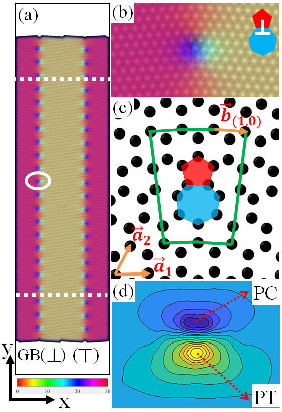
Figure 1: Structure of a simulated bicrystal containing armchair symmetric tilt grain boundaries (with tilt angle $\theta=7.34^{\circ}$). (a) Illustration of lattice orientation in the simulated system, where different colors correspond to different local crystallographic orientations (with color bar given at the bottom). The two dashed lines indicate the boundaries of the active zone. (b) Zoomed-in view of the circled region in (a). (c) The corresponding atomic structure of the $5|7$ dislocation in (b) and its Burgers vector $\vec{b}=(1,0)$. (d) Contour of the local strain $\varepsilon_{yy}$ distribution for (c), with the locations of peak compression (PC) and peak tension (PT) indicated.

The simulations are conducted for a 2D PFC system scaled by $L_{x}\times L_{y}$ (chosen as $512\Delta x\times 2048\Delta y$ in this work, corresponding to $13.6$ nm $\times$ $54.5$ nm) with periodic boundary condition in both directions, as illustrated in Fig. 1(a) with the use of lattice orientation contour [49]. The simulation box consists of three parts, with the first two being the solid crystalline regions coexisting with a third part of homogeneous phase (white margins of thickness $200\Delta y$ at each of the two vertical ends). Within the two solid regions that are stretched along the $y$ direction, the first part is set as the active zone (i.e., the middle area between the white dashed lines in Fig. 1(a), of initial size $L_{x}\times L_{y}^{0}=512\Delta x\times 1248\Delta y$ or $13.6$ nm $\times$ $33.2$ nm), in which the atomic structure mechanically deforms and relaxes following the external tensile load; the second part is the traction zones located at both ends of the solid where the loading is imposed (with fixed size $L_{x}\times L_{yt}=512\Delta x\times 200\Delta y$ at each side). The atomic density field in the traction zones is fixed and predetermined as $\phi_{\rm trac}$, which is the density profile of the corresponding regions when the whole system reaches equilibrium before the tensile deformation is applied. These two traction regions will then be moved adiabatically along the direction of tensile loading, while the system is subjected to the traction boundary condition [31] for which the free energy functional Eq. (1) is modified by $F\rightarrow F+F_{\rm ext}$, with $F_{\rm ext}=\int d\vec{r}M(\vec{r})[\phi(\vec{r})-\phi_{\rm trac}(\vec{r})]^{2}$ serving as free energy penalty. This penalty term is zero inside the active zone and the homogeneous regime (by setting $M(\vec{r})=0$), and is always positive in the traction regions (by setting e.g., $M(\vec{r})=2$) so that the associated density field $\phi_{\rm trac}$ can be imposed.

When the solid sheet is pulled at two ends along the $y$ direction, the length of the active zone is increased by $2\Delta y$ at each step. An interpolated scheme of the PFC model (i.e., the IPFC scheme [44]) is used to enable fast mechanical relaxation of the deformed system. At each numerical grid position it first estimates the updated value of the density field $\phi$ as a result of current-step mechanical deformation through a linear interpolation of the previous-step old density field, based on the assumption of local instantaneous elastic equilibration and the linear displacement in the limit of small strain increment; the system is then relaxed through PFC dynamics (i.e., Eq. (2)) to reach mechanical equilibrium before the next-step tensile deformation. More details of the algorithm as well as the way of evaluating engineering strain $\varepsilon_{e}$ and stress $\sigma_{e}$ during the deformation process are given in Ref. [44].

It is noted that the PFC model systems examined here are restricted to purely 2D, which would correspond to the scenario of epitaxial overlayer confined by the substrate such that effects of out-of-plane deformation are neglected. On the other hand, in real 3D systems out-of-plane corrugations should still have impacts on material properties, particularly for small-angle GBs (while such buckling would be significantly reduced for large GB misorientation angles with high dislocation density and/or by binding to the substrate) [50, 51]. For the case of tensile loading studied here, effects of any vertical variations are mitigated by the imposing of lateral stretching which tends to flatten the sheet. Thus the initial structure of out-of-plane deformation would be of less influence at larger applied strain, and is not expected to play a significant role (other than some small quantitative variations) on the behavior of plastic regime which is the focus of this work. It also would not affect the basic mechanisms of yielding or sample failure that will be identified below, particularly for any possible motion of dislocations which should still be mainly of 2D nature in a stretched epitaxial monolayer.

To generate the results of GBs, the PFC dynamic equation (2) is solved numerically through a pseudospectral method. Details of the numerical scheme are given in B. Note that the PFC model equation studied here is deterministic, without noise dynamics. The only possible randomness involved is in the initial condition setup. Our calculations show that different setup of initial noise in the system would not change the steady-state GB results that are used for the subsequent mechanical study, as the system always evolves to the same minimum-energy steady state; thus it would not affect the mechanical behavior and deformation properties of the system due to the deterministic PFC and IPFC dynamics used. In this work, unless otherwise specified, the model parameters used in the simulations are chosen as $\tau=1$, the numerical grid spacing $\Delta x=\Delta y=\pi/4$, time step $\Delta t=0.2$, and the strain rate $\dot{\varepsilon}_{e}=8.01\times 10^{-7}$, with the temperature parameter $\epsilon$ ranging from $-0.5$ to $-0.1$ (which corresponds to a temperature range from $3352$ K to $4278$ K based on the model parameterization described in A).

3 Results and Discussion

3.1 Structure and strain distribution of GBs

In most of our simulations the system is set up as a bicrystal containing two parallel symmetric GBs, each of misorientation angle $\theta$. Each GB separates two single crystalline graphene of orientations $\theta/2$ and $-\theta/2$, with the boundary line along the $y$ direction (i.e., the direction of tensile loading), as shown in Fig. 1(a). No preconstruction of detailed defect core structures and atomic configuration of GBs is needed in our PFC simulations; instead, the initial condition at the location of each GB is set up as a narrow vertical strip of supersaturated homogeneous phase connecting two misoriented single-crystalline regions. The PFC density of each homogeneous strip is of the same value as the average density of the solid regions, with a strip width of $20\Delta x$. We have varied the strip width from $10\Delta x$ to $20\Delta x$ and added different degree of initial noise in the system, all giving very similar results. The subsequent dynamic relaxation of the PFC equation leads to spontaneous solidification of this supersaturated strip which merges the two adjacent solid regions and forms a GB. The system then evolves to a steady state with minimum free energy, resulting in the stable GB configurations presented in Figs. 1 and 2. These GBs generated from the evolution of PFC density field consist of arrays of $5|7$ (penta-hepta) dislocation cores, consistent with the GB defect structure found in experiments and previous atomistic simulations of graphene. An example of $5|7$ disperse dislocation in a small-angle GB is given in Fig. 1(b)-(d), with Burgers vector $\vec{b}=(1,0)$ (based on the definition in Ref. [50]). Fig. 1(d) shows the contour of the corresponding local strain $\varepsilon_{yy}=\partial u_{y}/\partial y$, where $u_{y}$ is the $y$ component of the displacement field, as obtained through the method given in Refs. [52] and [53]. Regions of compressive vs. tensile strains can be identified for the two disclinations (5- vs. 7-membered rings), as well as the locations of peak compression (PC) and peak tension (PT) as indicated in Fig. 1(d). The midpoint between PC and PT can then be used to locate the exact position of the $5|7$ dislocation core.

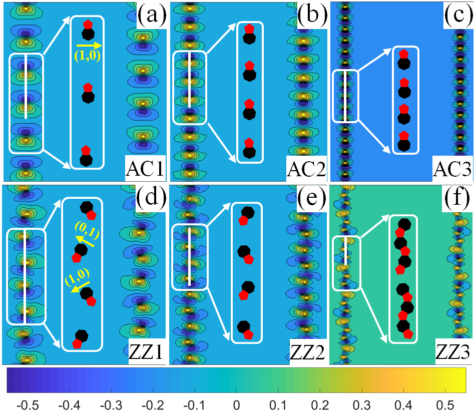
Figure 2: Spatial distribution of local strain $\varepsilon_{yy}$ for different graphene GBs, including armchair GBs with $\theta=7.34^{\circ}$ (denoted by AC1 in (a)), $13.17^{\circ}$ (AC2 in (b)), and $21.79^{\circ}$ (AC3 in (c)), and zigzag GBs with $\theta=8.61^{\circ}$ (ZZ1 in (d)), $13.17^{\circ}$ (ZZ2 in (e)), and $23.49^{\circ}$ (ZZ3 in (f)). Schematics of dislocations composed of pentagons (red) and heptagons (black) in the white boxed regions are shown in the middle of each panel. The cross-section profiles of $\varepsilon_{yy}$ along the GB line (corresponding to the white vertical lines in (a)–(f)) are given in (g), for different values of temperature parameter $\epsilon=-0.5$ ($T=3352$ K; solid black curves), $-0.4$ ($3584$ K; dashed red), $-0.3$ ($3815$ K; dotted green), $-0.2$ ($4047$ K; dot-dashed cyan), and $-0.1$ ($4278$ K; dotted blue).

Here we examine the detailed dynamics of low-, intermediate-, and high-angle symmetric tilt GBs subjected to the tensile loading parallel to the GB line. These include (i) armchair tilt GBs with misorientation angles $\theta=7.34^{\circ}$ (denoted by AC1), $13.17^{\circ}$ (AC2), and $21.79^{\circ}$ (AC3), where $\theta$ is measured between the armchair edges of the two adjoining grains, and (ii) zigzag tilt GBs with $\theta=8.61^{\circ}$ (ZZ1), $13.17^{\circ}$ (ZZ2), and $23.49^{\circ}$ (ZZ3), as measured between the two zigzag orientations of the grains. The corresponding GB structures and strain ($\varepsilon_{yy}$) contours before the tensile loading are presented in Fig. 2(a)–(f), showing an increase of dislocation density with larger $\theta$, as expected. For AC sheets, the GBs are composed of a periodic array of $5|7$ isolated dislocations with identical Burgers vector $\vec{b}=(1,0)$, and the spacing between neighboring $(1,0)$ dislocations decreases as $\theta$ increases (see Fig. 2(a)–(c)). For AC3 with large tilt angle $\theta=21.79^{\circ}$, there is a separation of only one atomic spacing between any pair of disperse $(1,0)$ dislocations, agreeing with the previous MD simulation results [18, 19, 54]. For zigzag sheets ZZ1 and ZZ2 at small and intermediate angles, each GB is constituted of alternating $(1,0)$ and $(0,1)$ dislocations whose Burgers vectors vary by $60^{\circ}$ in orientation (see Fig. 2(d), (e)). For ZZ3 with larger misorientation, each GB consists of a series of alternating $(1,0)+(0,1)+(1,0)$ and $(0,1)+(1,0)+(0,1)$ dislocation triplets (i.e., 3 connected $5|7$ dislocations), as shown in Fig. 2(f). The two neighboring triplets are separated by exactly one hexagon ring. A brief summary of these GBs examined in this work is given in Table 1 of A.

To further illustrate the spatial variation of strain around the dislocations, the one-dimensional cross-section profiles of $\varepsilon_{yy}$ along the GB line are plotted in Fig. 2(g), for all six armchair and zigzag GBs at different temperatures. The locations of strain peaks (PC vs. PT) are indicated, corresponding to the penta-hepta pairs of disclinations (see e.g., the shaded regions in Fig. 2(g)). As the misorientation angle increases from AC1 to AC3 or from ZZ1 to ZZ3, the distance between neighboring dislocation cores decreases due to higher dislocation density; however, for AC GBs (AC1 to AC3) the distance between the two constituent disclinations of each dislocation (i.e., between PC and PT positions of the shaded region), which is proportional to the size of dislocation core region, remains almost unchanged, although the corresponding magnitude of strain variation along the GB direction becomes smaller. By contrast, for ZZ GBs as $\theta$ increases (ZZ1 to ZZ3) both the dislocation core size and strain variation magnitude decrease. This difference is attributed to the fact that different from the AC GBs that are characterized by arrays of a single type of $(1,0)$ dislocations, the dislocations in ZZ GBs are of mixed type (i.e., $(1,0)$ and $(0,1)$), leading to different degree of elastic interaction between dislocations along the GB line particularly the cancellation of stress fields between nearby or connected dislocations [55, 56]. Similar results of defect structures and strain distribution in the absence of external deformation are obtained at different temperatures (see e.g., close-to-overlapped plots in Fig. 2(g) for different temperature values). They play an important role on determining the mechanical properties of GBs samples under external loading, as will be detailed below.

3.2 Effects of uniaxial tension: Brittle failure behavior

Figures 3–5 show the results of deformation or fracture behavior and mechanical properties of these armchair and zigzag GBs after the imposing of uniaxial tensile loads (with direction parallel to the GBs), which are consistent with those found in previous experiments and MD simulations. An example of the stress-strain relation at $\epsilon=-0.5$ (corresponding to $T=3352$ K) is presented in Fig. 3, for both AC and ZZ GBs under uniaxial tension. A brittle-type failure behavior is found for these symmetric GBs of different misorientation angles, similar to previous MD results for graphene calculated at low (or $0$ K) temperature with loading direction either parallel or perpendicular to the GB [18, 19, 20], and also to the corresponding PFC calculations conducted at a low temperature of $111$ K ($\epsilon=-1.9$) in B.

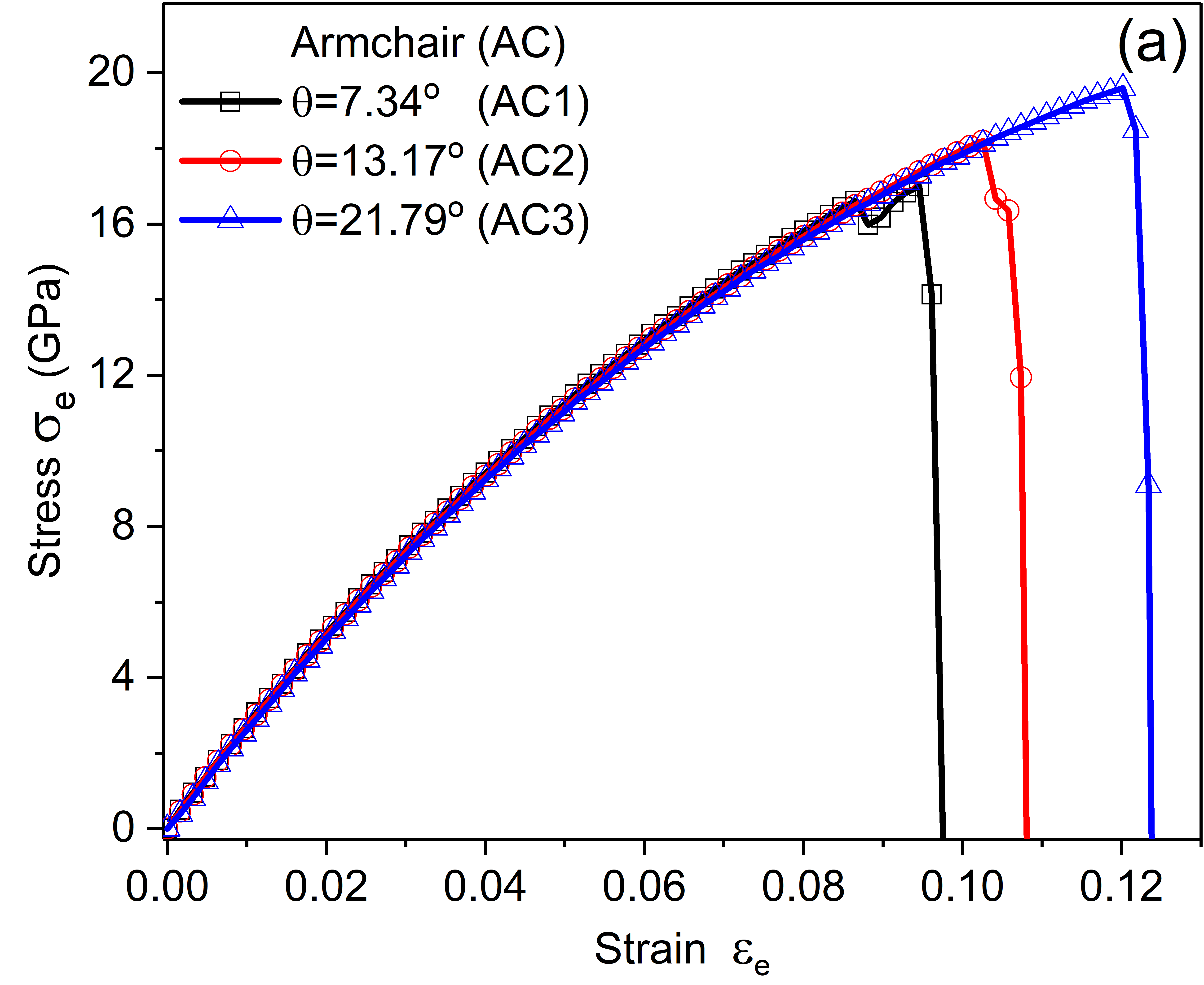
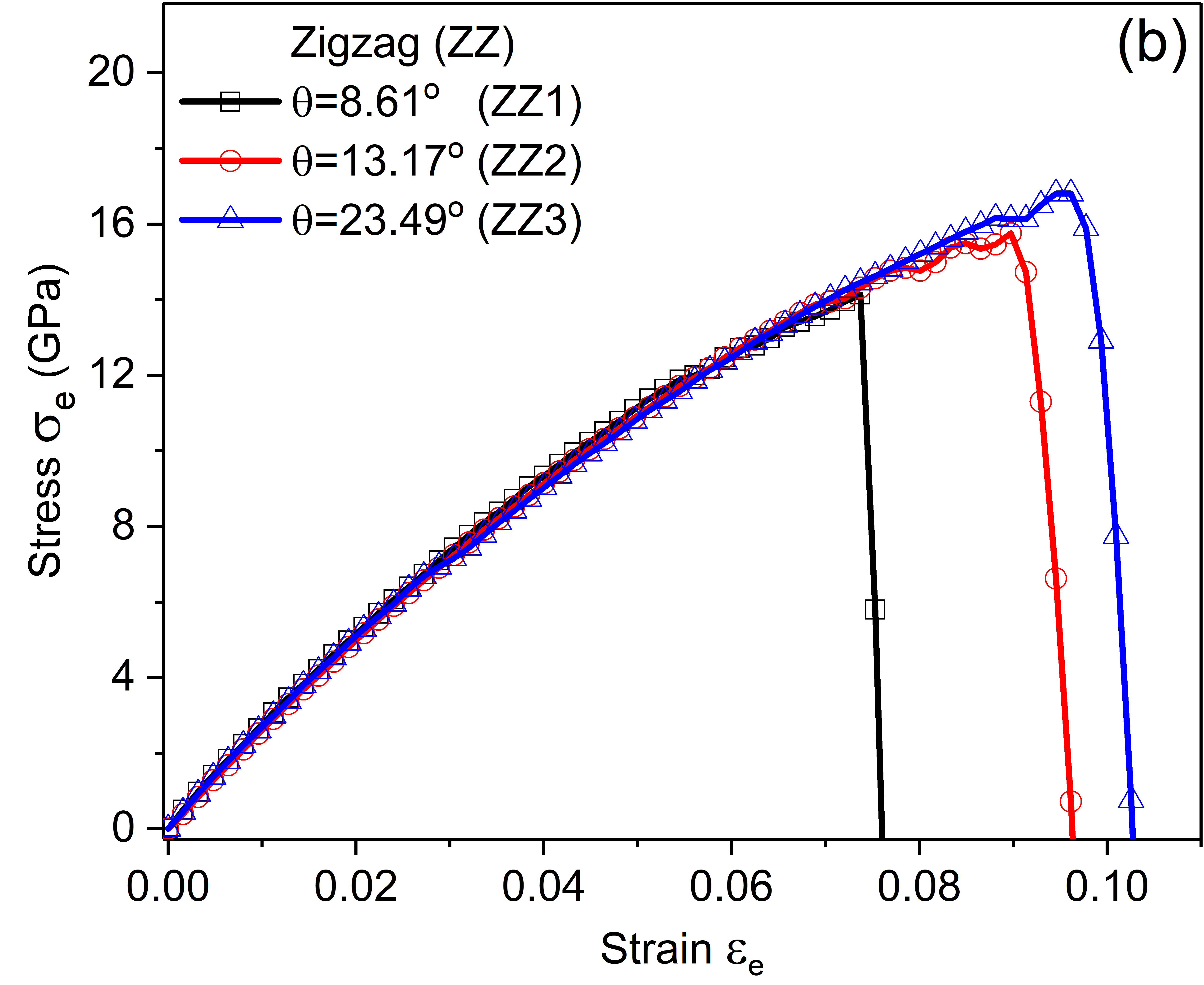
Figure 3: Stress-strain curves for (a) AC and (b) ZZ sheets at $\epsilon=-0.5$ ($T=3352$ K) under uniaxial tension applied parallel to the GBs.

In both cases of AC and ZZ GBs with regularly distributed $5|7$ dislocations studied here, larger tilt angles $\theta$ correspond to stronger GBs with larger strain value at failure and higher ultimate strength (defined as the maximum tensile stress during deformation; see Fig. 3(a), (b) and Fig. 4(a) at high temperatures and also Fig. 15 in B at a low temperature), which qualitatively agrees with previous MD [18, 19, 20] and experimental [7] findings. This can be attributed to higher density of dislocation arrays at larger $\theta$, which leads to a larger degree of mutual cancellation of dislocation stress fields and thus smaller prestrain [55], yielding larger failure strain and GB strength. More quantitative details will be given below. On the other hand, as shown in Fig. 4(b) values of Young’s modulus $Y$, as calculated from the small-strain linear part of the stress-strain curves, depend weakly on the misorientation angle and are close to that of the pristine sample (e.g., at $\epsilon=-0.5$ ($T=3352$ K) $Y$ values of various GBs are close to the value of $284$ GPa obtained for the corresponding armchair single crystal of the same size). This is consistent with experimental measurements showing very limited influence of grain boundaries on the elastic moduli of graphene [4, 5]. We note that values of stress and Young’s modulus calculated here are much smaller than those reported in previous MD simulations, which is due to the much higher temperature range examined in this work. If using low temperatures (see Fig. 15 at $T=111$ K in B for both AC and ZZ GBs and also Fig. 14 in A for pristine graphene), the values obtained from our PFC modeling are comparable to atomistic simulation results.

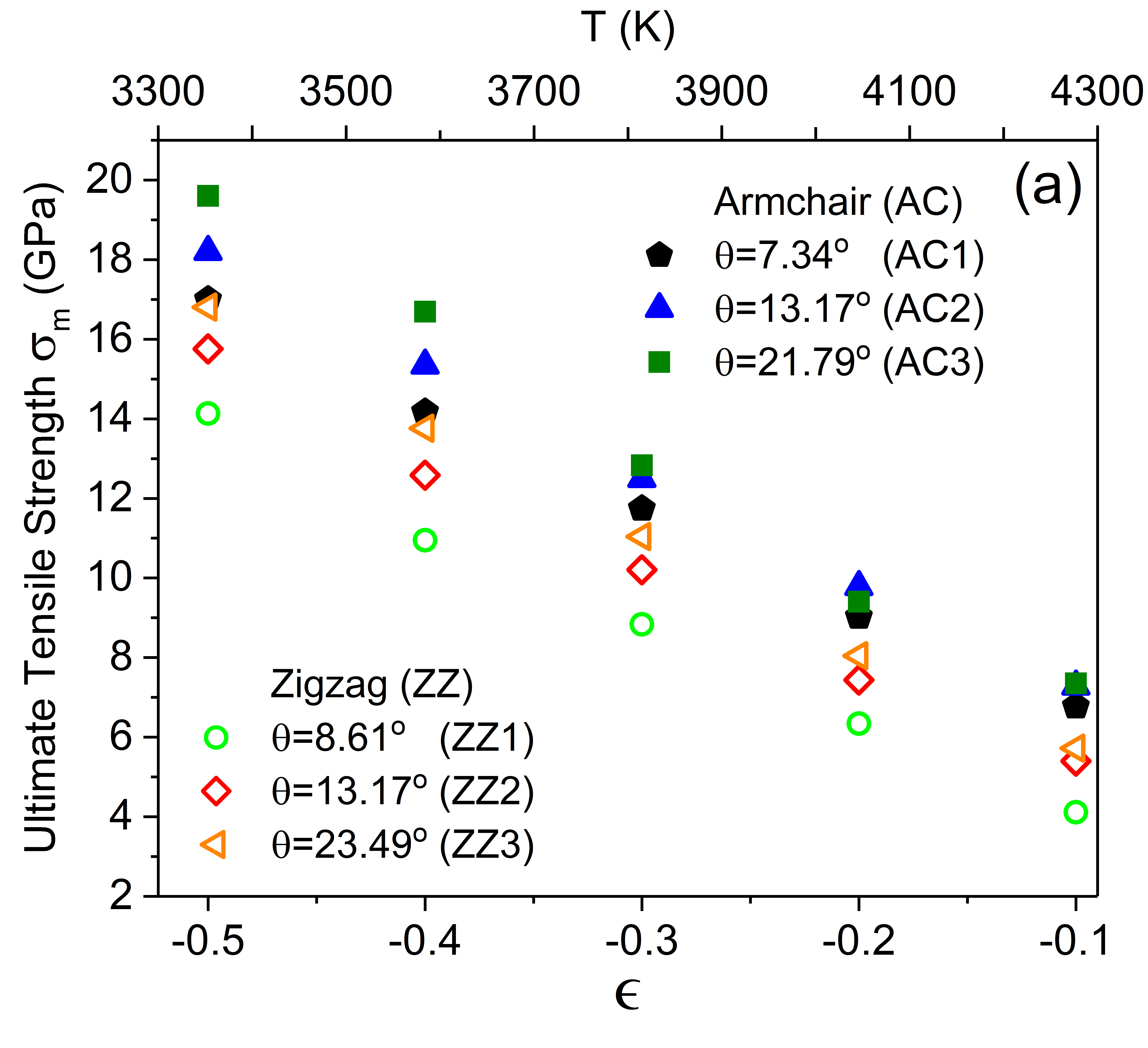
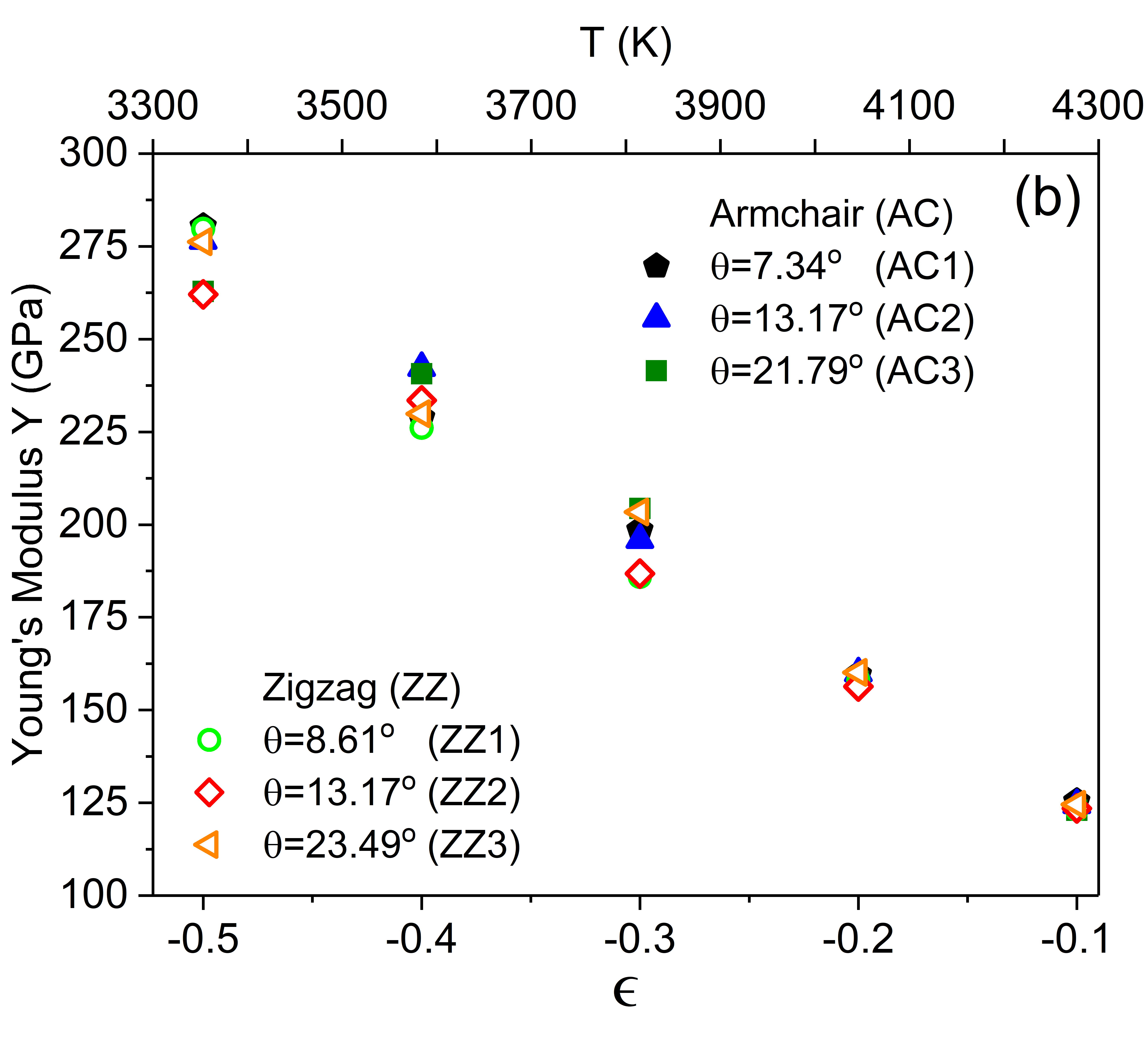
Figure 4: (a) Ultimate tensile strength and (b) Young’s modulus as a function of temperature for various AC and ZZ GBs.

Snapshots of the corresponding atomic structures during deformation and fracture are given in Fig. 5, for both AC and ZZ sheets. Our PFC simulations show that failure or cracking of the GB sheet originates from the breaking of rings at or next to $5|7$ dislocations and hence the formation of nanovoids at the GB, before the cracks propagate into the interior of the grain. This scenario well agrees with experimental observation [6, 7] showing crack propagation inside the grain following the armchair or zigzag lattice direction but not along the GB line, as seen in our results of Fig. 5 and also Fig. 15 in B. Our finding also agrees with previous atomistic simulations of graphene where the bond breaking at the defect rings of GBs was observed in MD as the initiation of sample failure [18, 21], and the increase of ultimate strength with the GB tilt angle has been attributed to the reduction of initial prestrain within the defect rings or bonds as the angle increases, based on MD and quantum DFT calculations [18]. As indicated in Fig. 2(g) and discussed in Sec. 3.1, our PFC results give a similar trend of preexisting strain around dislocation cores before any tensile deformation is applied: For AC sheets with GB angle $\theta$ increasing from $7.34^{\circ}$ (AC1), $13.17^{\circ}$ (AC2), to $21.79^{\circ}$ (AC3), the strain amplitude between the penta-hepta disclination pair is measured as 7.93%, 6.92%, and 5.21% respectively; Similarly, for ZZ sheets the strain amplitude estimated in the regions of Fig. 2(g) decreases from 5.91%, 5.74%, to 5.6% when $\theta$ increases from $8.61^{\circ}$ (ZZ1), $13.17^{\circ}$ (ZZ2), to $23.49^{\circ}$ (ZZ3). This decrease of preexisting strain caused by dislocation defect rings results in the enhancing of GB strength and larger failure strain with higher tilt angle, as seen in Figs. 3, 4(a), and 15 and consistent with MD results for graphene [18].

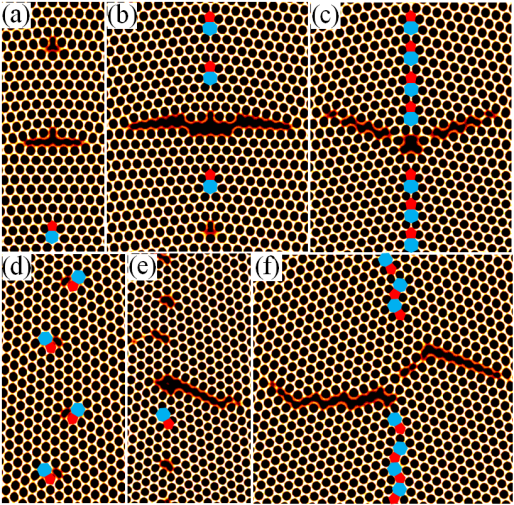
Figure 5: Atomic structures at the stage of sample failure in AC and ZZ sheets at $\epsilon=-0.5$ ($T=3352$ K), for (a) AC1 at applied engineering strain $\varepsilon_{e}=9.78\%$, (b) AC2 at $10.98\%$, (c) AC3 at $12.42\%$, (d) ZZ1 at $7.05\%$, (e) ZZ2 at $9.38\%$, and (f) ZZ3 at $10.26\%$.

Interestingly, a new and different phenomenon of deformation dynamics is observed for ZZ GBs at low enough angle, e.g., ZZ1 sheet with $\theta=8.61^{\circ}$, as compared to the intermediate- and high-angle ZZ GBs (ZZ2 and ZZ3 in Fig. 5(e) and (f)). As shown in Fig. 5(d), for this low-angle GB characterized by well-separated $(1,0)$ and $(0,1)$ dislocations, although the failure still initiates around the GB $5|7$ dislocations the subsequent deformation dynamics is featured by the motion (mostly glide) of each individual dislocation bound together with its connected nanovoid. The glide directions of $(1,0)$ and $(0,1)$ dislocations are opposite to each other, both perpendicular to the external pulling direction, leading to the splitting of the GB dislocation array into two sub-arrays of $(1,0)$ and $(0,1)$ types respectively. It is noted that although these disperse $(1,0)$ and $(0,1)$ dislocations have been examined in MD [56, 51], first-principles DFT [50, 57], and 2D PFC [38, 41] studies, the focus there was on the corresponding GB energies without external stress. For the case of tensile deformation and fracture, in previous MD simulations of low enough tilt angles [18, 19, 20, 22] the ZZ GBs with $(1,0)+(0,1)$ paired dislocations (i.e., the bound $5|7|5|7$ pairs) were studied instead, which yields the normal behavior of cracking that initiates at and propagates from the defect locations without the motion of dislocations (similar to that of AC and ZZ2, ZZ3 GBs shown in Fig. 5), a scenario different from the failure dynamics of GB disintegration observed here in the small-angle ZZ1 sheet. For 2D planar systems as examined in this work, it has been found by DFT [50] and combined MD and PFC [41] calculations that without external deformation, the lowest-energy structures of intermediate- and low-angle ZZ GBs are those of $(1,0)$ and $(0,1)$ disperse $5|7$ dislocations, instead of the paired ones, consistent with our finding here. Even when out-of-plane deformations are considered, recent results combining MD and Read-Shockley-type dislocation model indicated that this disperse $(1,0)$ and $(0,1)$ structure is also the lowest-energy state of ZZ GBs at small enough angles (e.g., $\theta\simeq 10^{\circ}$) [56].

3.3 Effects of uniaxial tension: Plastic flow at ultrahigh temperature

We have further investigated the influence of temperature on the mechanical properties and deformation dynamics of graphene grain boundaries. Fig. 4 shows the variations of the ultimate tensile strength $\sigma_{m}$ and Young’s modulus $Y$ with respect to temperature (ranging between $\epsilon=-0.5$ ($T=3352$ K) and $-0.1$ ($4278$ K)) for both AC and ZZ GBs. Clearly, with the increase of temperature the ultimate strength $\sigma_{m}$ of AC and ZZ sheets decreases monotonously (Fig. 4(a)), similar to the temperature dependence of the failure strength of graphene GBs obtained in MD [22] although here the range of temperatures examined is much higher. In addition, the result of larger $\sigma_{m}$ at higher GB angle $\theta$ holds for different temperatures given the effect of prestrain described above, although the variation becomes smaller at higher temperature. For Young’s modulus $Y$, it is found to also decrease with the increase of temperature for both AC and ZZ sheets (Fig. 4(b)), consistent with the MD results for pristine graphene [46]. Across the temperature range examined in this study, only weak dependence of $Y$ on the tilt angle $\theta$ is obtained, especially for ultrahigh temperatures.

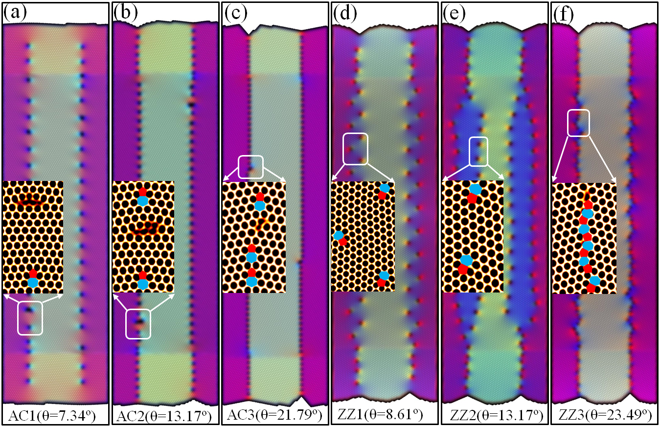
Figure 6: Spatial distribution of local lattice orientation at ultrahigh temperature ($\epsilon=-0.1$ with $T=4278$ K), for (a) AC1 at $\varepsilon_{e}=8.56\%$, (b) AC2 at $9.60\%$, (c) AC3 at $10.07\%$, (d) ZZ1 at $5.45\%$, (e) ZZ2 at $7.13\%$, and (f) ZZ3 at $7.18\%$. The atomic structure of the boxed region is shown inside each panel.

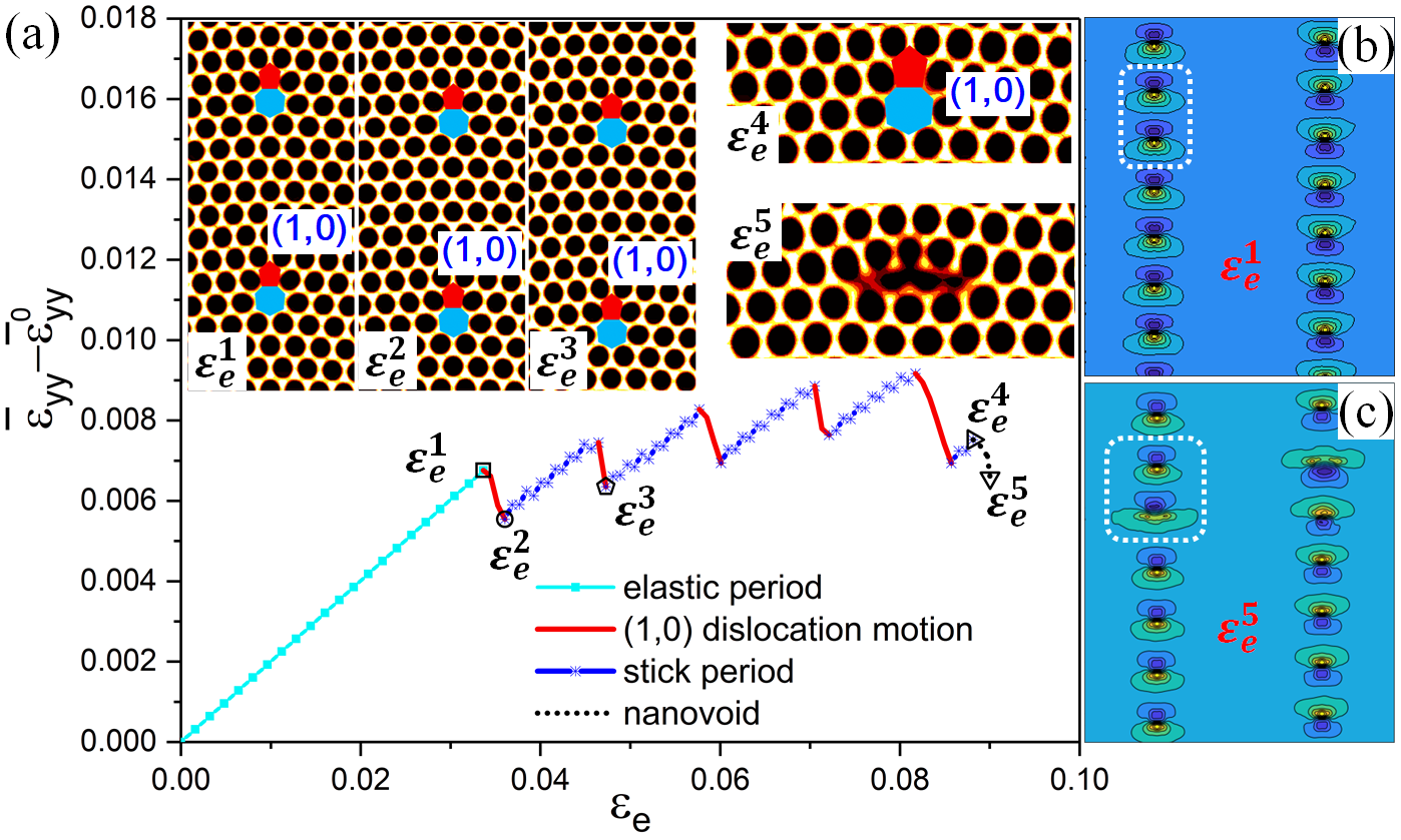
Figure 7: (a) Change of average local strain, $\bar{\varepsilon}_{yy}-\bar{\varepsilon}_{yy}^{0}$, as a function of applied strain $\varepsilon_{e}$ for AC1 sheet at $\epsilon=-0.1$ ($T=4278$ K). The insets show the dynamic process of dislocation motion and the formation of nanovoid, corresponding to snapshots at $\varepsilon_{e}^{1}=3.37\%$, $\varepsilon_{e}^{2}=3.61\%$, $\varepsilon_{e}^{3}=4.73\%$, $\varepsilon_{e}^{4}=8.81\%$, and $\varepsilon_{e}^{5}=8.99\%$. (b) and (c) give the contours of the local strain $\varepsilon_{yy}$ distribution at $\varepsilon_{e}^{1}$ and $\varepsilon_{e}^{5}$ respectively, with the boxed region corresponding to the two dislocations shown in the insets of (a).

Details of sample failure and deformation dynamics at ultrahigh temperature $\epsilon=-0.1$ (with $T=4278$ K, close to the melting point of graphene which corresponds to $\epsilon=0$ and $T_{m}=4510$ K [9]) are presented in Figs. 6–9, showing qualitatively different behaviors of sample yielding as compared to those of relatively lower temperature given above in Sec. 3.2. For all the AC GBs a similar failure behavior, characterized by the formation of nanovoids, is found at late stages, with some snapshots shown in Fig. 6 (a)–(c). Different from the lower-temperature results, here plastic deformation occurs after the beginning elastic regime and is characterized by a jerky or serrated flow behavior and stick and climb-glide type dislocation motion (i.e., alternating periods of GB dislocation migration and temporary stoppage or pinning), with the corresponding yield process detailed in Fig. 7 for the example of AC1 sheet. This jerky plastic flow can be identified from the result of the local strain $\varepsilon_{yy}$ averaged within the active zone of simulation, i.e., $\bar{\varepsilon}_{yy}$. Its variation with respect to the initial average strain $\bar{\varepsilon}_{yy}^{0}$ at $\varepsilon_{e}=0$, $\bar{\varepsilon}_{yy}-\bar{\varepsilon}_{yy}^{0}$, is plotted against the imposed engineering strain $\varepsilon_{e}$ in Fig. 7(a). After the imposed strain reaches the yield point with strain value $\varepsilon_{e}^{Y}$ (e.g., $\varepsilon_{e}^{Y}=\varepsilon_{e}^{1}=3.37\%$ in Fig. 7), corresponding to the end of elasticity regime and the onset of jerky plasticity, a steep drop in the $\bar{\varepsilon}_{yy}$ curve occurs. This drop of local strain/stress is attributed to the glide-climb motion of all the $5|7$ dislocations at the GB simultaneously, as can be seen by comparing the corresponding structure snapshots at the two ends of the drop $\varepsilon_{e}=\varepsilon_{e}^{1}$ and $\varepsilon_{e}^{2}$ in the insets of Fig. 7(a). During this period each dislocation climbs down one atomic step and also glides one atomic step to the right. After then dislocations are pinned by the underlying lattice structure (i.e., the effect of Peierls barriers) and become immobile, and the applied uniaxial stress/strain accumulates in the system, with the average build-up rate similar to that of the elastic regime (see the blue stick period in Fig. 7(a)) given the absence of dislocation motion. Once the pinning barriers are overcome by the accumulated stress the unpinned dislocations move again, by further climbing down one atomic step but gliding one step back to the left (i.e., the opposite direction of glide compared to the previous period of motion; see the $\varepsilon_{e}^{3}$ inset). This causes the second steep drop of the average local strain. Compared this state (at $\varepsilon_{e}=\varepsilon_{e}^{3}$) to the onset of plastic deformation (at $\varepsilon_{e}=\varepsilon_{e}^{1}$), the net motion of dislocation is the climb of two atomic steps down, but no net glide. This procedure of stick-and-climb-glide is repeated until the GB failure occurs, showing as the nanovoid formation at some GB dislocations (see $\varepsilon_{e}^{4}$ vs. $\varepsilon_{e}^{5}$ in Fig. 7(a)). The corresponding spatial distribution of the local strain $\varepsilon_{yy}$ is given in Fig. 7(b) and (c), at the onset of jerky plasticity and the formation of nanovoid respectively. Note that this behavior of dislocation migration only appears at high enough temperature, with fast enough atomic diffusion process and low enough defect pinning barriers such that the dislocation motion would occur at early enough stage before sample failure (i.e., before nanovoids form at the GB).

The situation for ZZ GBs at this ultrahigh temperature is more complicated, with the deformation processes depending on the GB misorientation angle and details of the dislocation structure (see Fig. 6 (d)–(f) for some snapshots at large strains with $\epsilon=-0.1$ or $T=4278$ K). For low and intermediate angles (ZZ1 and ZZ2 GBs with $\theta=8.61^{\circ}$ and $13.17^{\circ}$) a similar behavior is found, which however is different from the high-angle one (ZZ3 with $\theta=23.49^{\circ}$). At large enough strains (beyond the yield point), in both ZZ1 and ZZ2 sheets the motion of dislocations under the tensile load causes the split of the dislocation array at each GB along the direction perpendicular to the external loading, leading to two sub-arrays of dislocations of $(1,0)$ and $(0,1)$ types respectively. This is analogous to the phenomenon of collective dislocation separation from the GBs (see Fig. 6 (d) and (e)), but different from the GB disintegration at lower-temperature ZZ1 GBs (Fig. 5(d) with $\epsilon=-0.5$ or $T=3352$ K) which instead occurs after GB failure and is accompanied by the motion of dislocation-bound nanovoids.

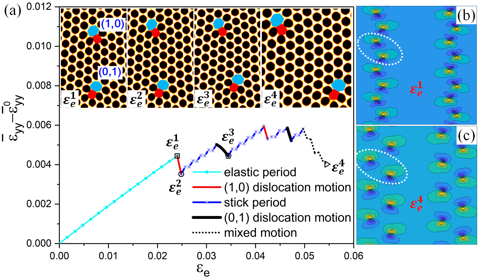
Figure 8: (a) Change of average local strain, $\bar{\varepsilon}_{yy}-\bar{\varepsilon}_{yy}^{0}$, as a function of applied strain $\varepsilon_{e}$ for ZZ1 sheet at $\epsilon=-0.1$ ($T=4278$ K). The insets show the dynamic process of dislocation migration, corresponding to snapshots at $\varepsilon_{e}^{1}=2.40\%$, $\varepsilon_{e}^{2}=2.48\%$, $\varepsilon_{e}^{3}=3.45\%$, and $\varepsilon_{e}^{4}=5.45\%$. (b) and (c) give the contours of the local strain $\varepsilon_{yy}$ distribution at $\varepsilon_{e}^{1}$ and $\varepsilon_{e}^{4}$ respectively, with the boxed region corresponding to the two dislocations shown in the insets of (a).

Details of the deformation dynamics for ultrahigh-temperature ZZ1 GBs are given in Fig. 8, showing the behavior of jerky plastic flow similar to that of AC sheets, as seen from the corresponding strain curve of $\bar{\varepsilon}_{yy}$ vs. $\varepsilon_{e}$. However, in the plastic regime the dynamics of mobile dislocations is different. As shown in Fig. 8(a), during the first drop of local strain/stress from the yield point $\varepsilon_{e}=\varepsilon_{e}^{1}$ to $\varepsilon_{e}^{2}$ the $(1,0)$ dislocations migrate via a mixed motion of glide and climb (one atomic step leftward and one step upward for the example of Fig. 8(a)), while the $(0,1)$ dislocations remain immobile. After the subsequent stick period with the pinning of both types of defects, the next drop in strain curve occurs, which is caused by the glide and climb of $(0,1)$ dislocations (one atomic step rightward and one step upward if comparing $\varepsilon_{e}^{3}$ and $\varepsilon_{e}^{2}$ inset panels), while the $(1,0)$ dislocations keep immobile this time. The repeat of this procedure, as featured by the alternative motion of one type of dislocations intermitted by a temporary period of defect pinning, results in the splitting of each GB dislocation array into two sub-arrays as described above and also illustrated in Fig. 8 (b) vs. (c) in terms of local strain distribution. Compared to the case of AC GBs shown in Fig. 7, here the jerky behavior of plastic flow is less regular, with shorter stick/pinning periods as time (or $\varepsilon_{e}$) increases. This can be attributed to larger degree of dislocation glides for this type of ZZ GBs (given its different dislocation structure and GB strain distribution compared to the AC GBs; see Fig. 2) and the interaction between dislocations separated from two neighboring GBs. At late times (with large applied $\varepsilon_{e}$) the dislocation sub-arrays from two different GBs will annihilate, leading to a fast decrease of system elastic energy and stress.

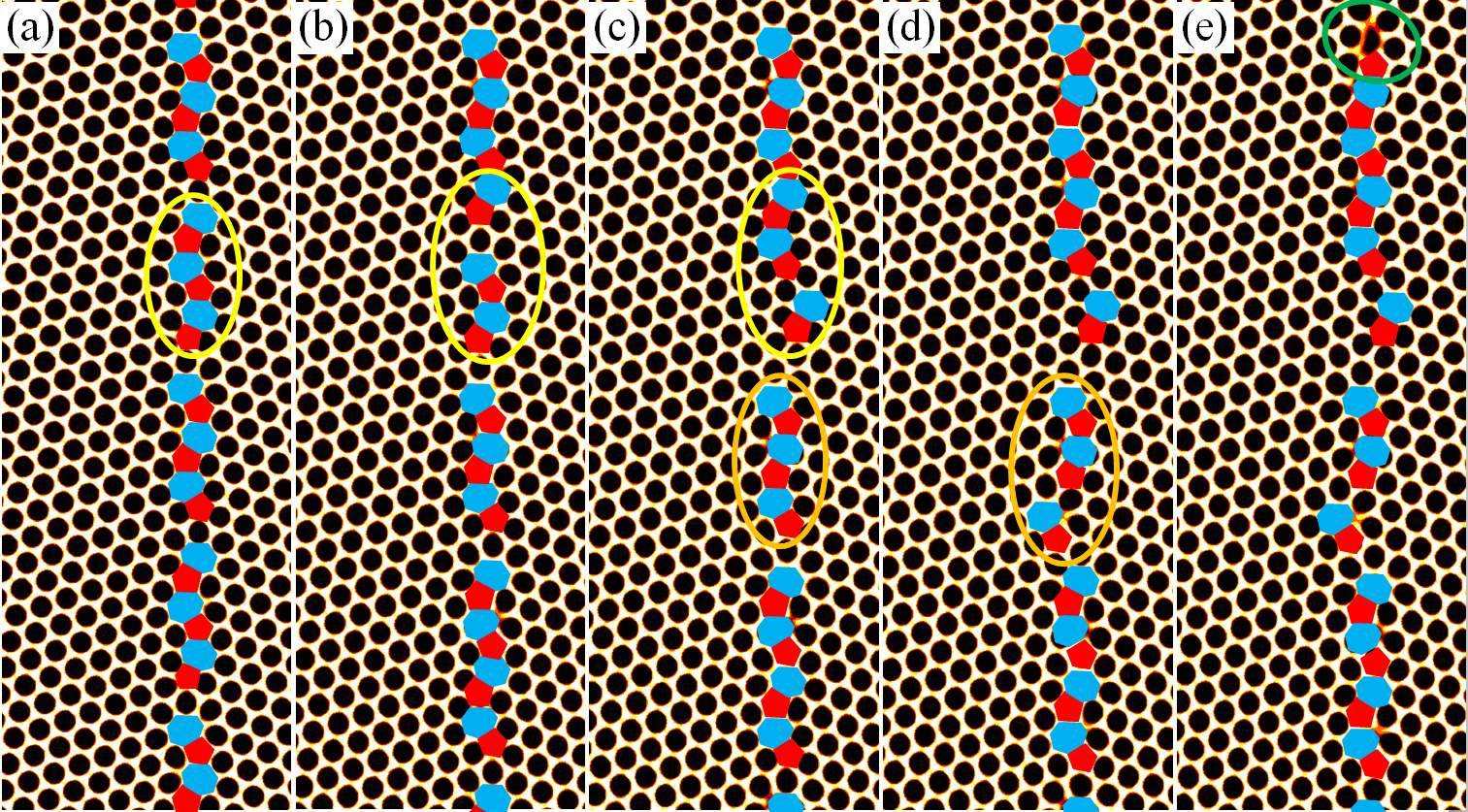
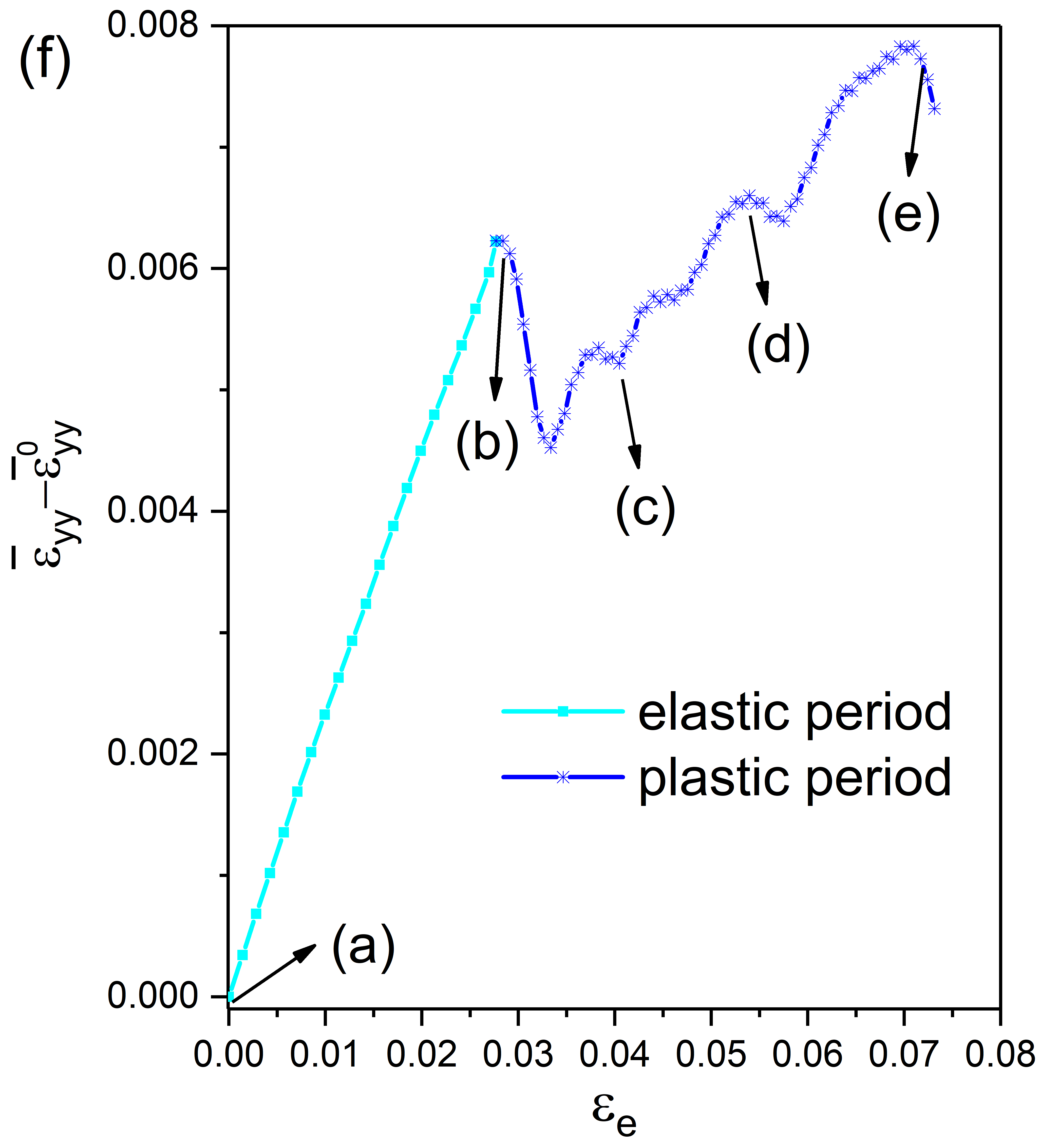
Figure 9: Snapshots of the structural evolution process of ZZ3 GB, at $\epsilon=-0.1$ ($T=4278$ K) and $\varepsilon_{e}=0$ (a), $2.91\%$ (b), $4.12\%$ (c), $5.11\%$ (d), and $7.18\%$ (e). Pentagons and heptagons are colored in red and blue, respectively. Only a portion of the simulated system is shown here. The average local strain vs. $\varepsilon_{e}$ is given in (f).

Among the ZZ sheets the detailed dynamics of dislocations highly depends on the type of GB defect structure. As shown in Fig. 2(f) and also Fig. 9(a), the high-angle ZZ3 GB is composed of a different type of dislocation array (i.e., connected dislocation triplets) and exhibits different strain distribution as compared to the low/intermediate-angle ZZ1 and ZZ2 GBs with disperse $(1,0)$ and $(0,1)$ $5|7$ defects, leading to more complex deformation behavior under the imposed tension. An example of a series of dislocation dynamics under tensile stress is illustrated in Fig. 9 (a)–(e). Beyond the yield point a $(0,1)+(1,0)+(0,1)$ dislocation triplet breaks up within this portion of the GB shown in the figure, and its top $(0,1)$ dislocation glides and climbs up one atomic step to join the neighboring dislocation cluster (see the circled region in Fig. 9 (a) and (b)). Once the applied stress is built up and exceeds the pinning barrier, the remaining pair breaks up again, where the $(1,0)$ dislocation migrates one step to connect with the upper cluster (see the upper circle in Fig. 9(c)). Further increasing the stress leads to the disintegration of another dislocation triplet, i.e., the $(1,0)+(0,1)+(1,0)$ one circled in the lower part of Fig. 9 (c) and (d). At high enough external strain/stress nanovoids form at the GBs, as indicated in Fig. 9(e), corresponding to the occurrence of sample failure. Similar procedure of dislocation triplet break-up and single dislocation migration occurs in various segments of the GB (see also Fig. 6(f)), and the corresponding plot of strain curve showing a jerky plastic flow is given in Fig. 9(f).

A similar behavior of jerky plasticity has been obtained in previous experimental and MD studies of GBs in 3D nanowires or micropillars under uniaxial compression [58, 59], although with different underlying mechanisms. In those 3D cases new dislocations nucleate inside the system under large enough built-up stress and then migrate, while the stick period (without any dislocation activities) is caused by either dislocation starvation (which corresponds to larger amplitude of jerky behavior) or pinning [58]. In the 2D system studied here, no nucleation of additional dislocations is found, and all the dislocations are those from the initial state; the phenomenon of high-temperature jerky plastic flow originates purely from stress-induced dislocation motion and temporary lattice pinning.

3.4 The brittle-to-ductile transition

To summarize the effect of system temperature on the GB deformation dynamics, we plot the strain-strain curves of $\bar{\varepsilon}_{yy}$ vs. $\varepsilon_{e}$ in Fig. 10 for all the GBs examined here with temperature ranging from $\epsilon=-0.5$ ($T=3352$ K) to $-0.1$ ($4278$ K). The corresponding stress-strain curves are given in Fig. 11. At low enough temperatures ($T\lessapprox 3352$ K) the brittle-type behavior of fracture is observed, analogous to previous results of MD simulations. As temperature increases a transition to plastic or ductile behavior occurs, particularly the behavior of jerky plastic flow at high enough temperatures (e.g., $T=4278$ K studied above). This phenomenon of jerky plasticity can be seen from the serrated or seemingly irregular curves of the stress-strain relation given in Fig. 11. Each turning point in the stress-strain curve can be matched to the corresponding point of the strain-strain curve in Fig. 10, which in turn has been one-to-one correlated to the associated stick and climb-glide motion of GB dislocations as described in detail in Sec. 3.3 for both AC and ZZ GBs (see also Figs. 7–9).

Usually the brittle-to-ductile transition is accompanied by the generation of sufficient amount of new dislocations from existing sources inside the sample. However, in the 2D system studied here no such dislocation generation or nucleation is found; instead, the plastic deformation, particularly jerky plasticity, develops as long as the GB dislocations are able to migrate under large enough external stress/strain, before the atomic-ring breaking and the nucleation of nanovoids would have time to initiate at the GB. The motion of dislocations (both glide and climb) can occur even when being limited around the GB region, as seen in AC and ZZ3 GBs (Figs. 7 and 9), under the condition that the individual GB dislocations or dislocation clusters (e.g., pairs or triplets) are separated from each other and the temperature is high enough such that pinning of the lattice and binding of nearby dislocations via elastic interaction could be overcome by large enough atomic mobility under external stress. This can be made possible in graphene-type 2D systems which, different from more complicated 3D cases, do not involve dislocation loops and intersection and are hence less restricted in terms of dislocation motion.

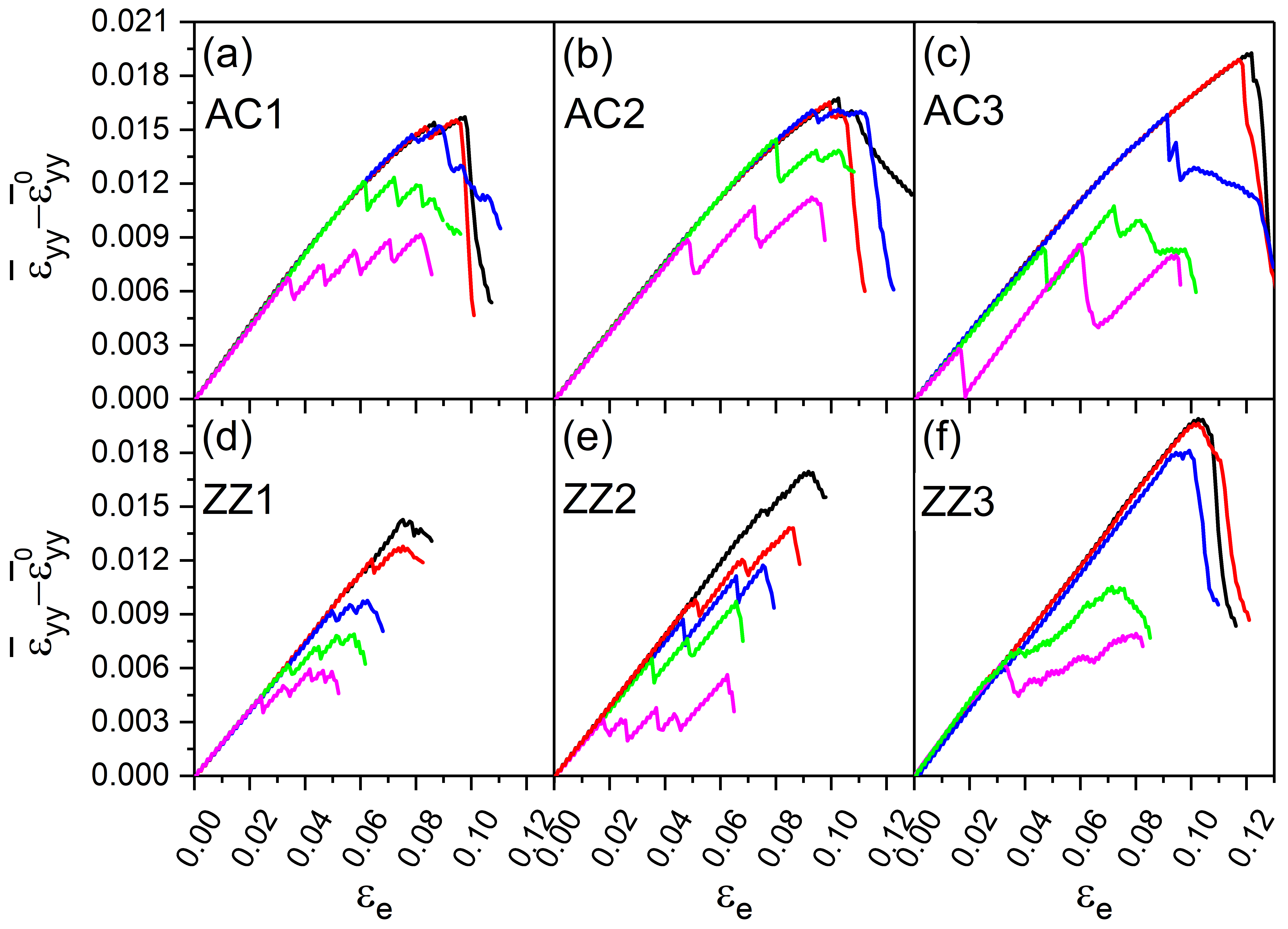
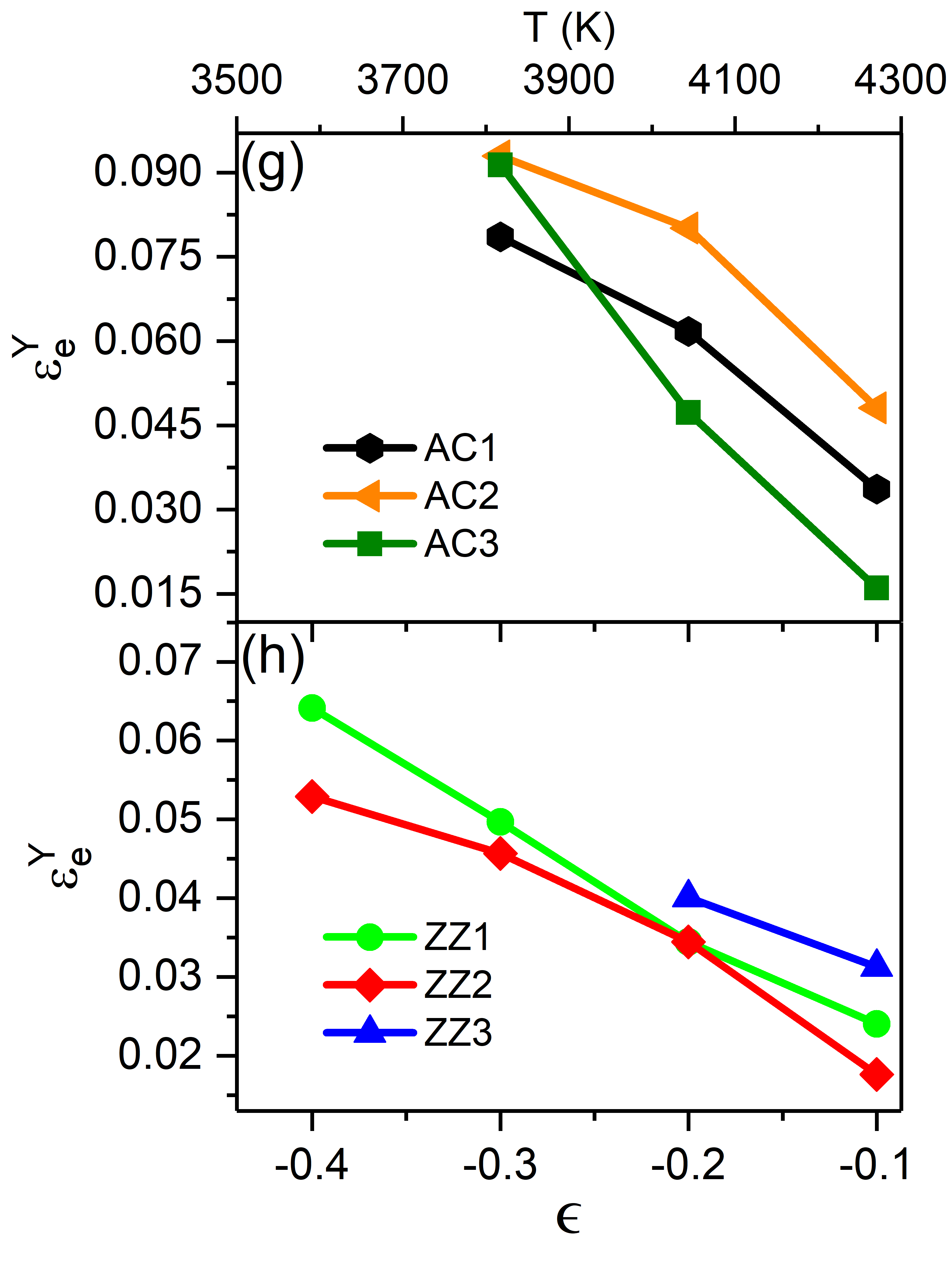
Figure 10: (a)–(f): Change of average local strain, $\bar{\varepsilon}_{yy}-\bar{\varepsilon}_{yy}^{0}$, as a function of $\varepsilon_{e}$ for AC and ZZ sheets with the direction of tensile loading parallel to the GBs, at different values of temperature $\epsilon=-0.5$ ($T=3352$ K; black), $-0.4$ ($3584$ K; red), $-0.3$ ($3815$ K; blue), $-0.2$ ($4047$ K; green), and $-0.1$ ($4278$ K; magenta) from top to bottom. (g) and (h): Values of $\varepsilon_{e}$ at the yield point, $\varepsilon_{e}^{Y}$, as a function of temperature, for AC and ZZ GBs respectively.

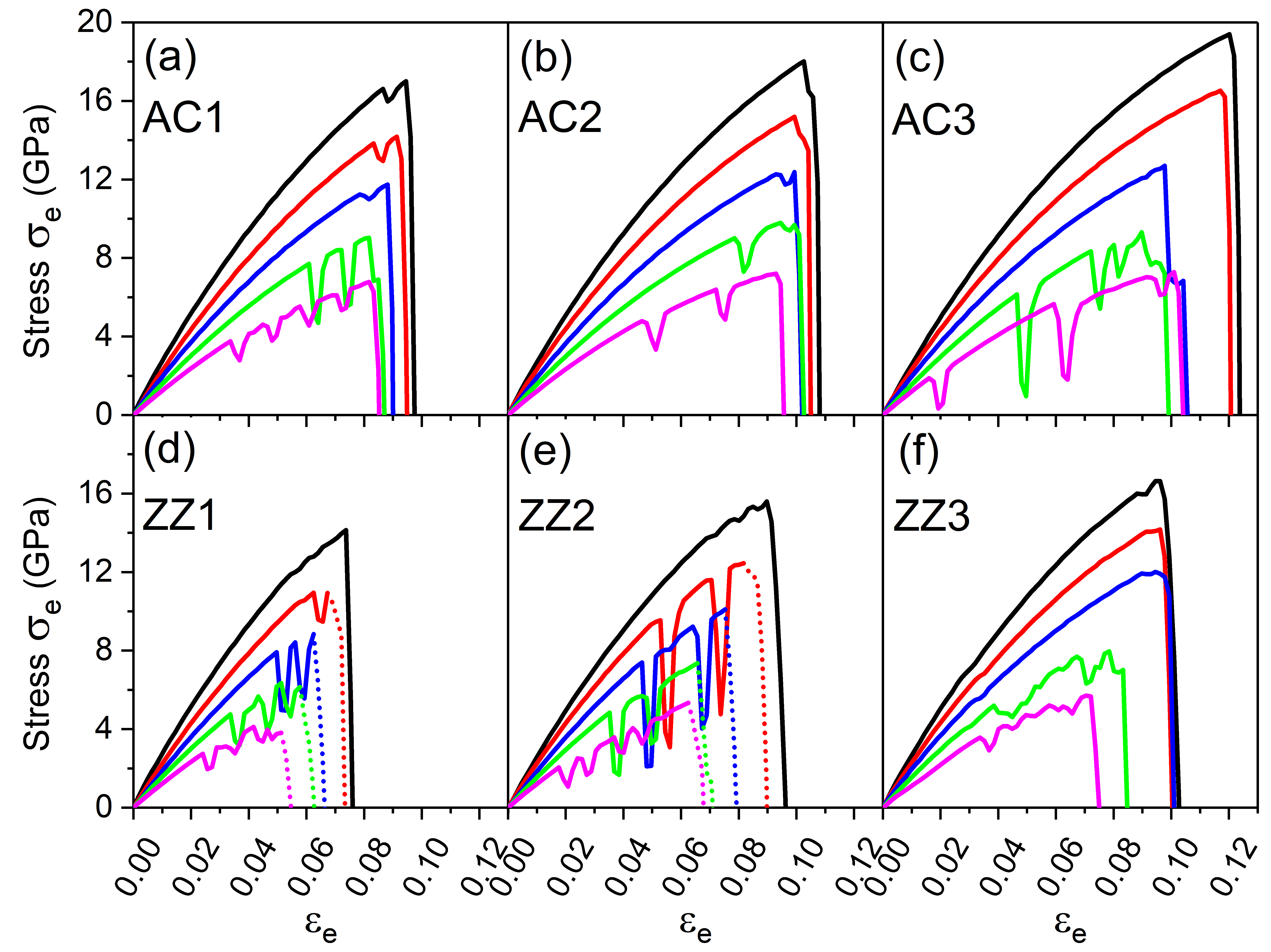
Figure 11: Stress-strain curves for AC ((a)–(c)) and ZZ ((d)–(f)) sheets with the direction of tensile loading parallel to the GBs, at different values of temperature $\epsilon=-0.5$ ($T=3352$ K; black), $-0.4$ ($3584$ K; red), $-0.3$ ($3815$ K; blue), $-0.2$ ($4047$ K; green), and $-0.1$ ($4278$ K; magenta) from top to bottom. The dotted lines in (d) and (e) correspond to fast decrease of system elastic energy and stress caused by the annihilation of dislocation sub-arrays separated from two different GBs given the finite system size in the simulation.

Details of this brittle to ductile/plastic transition would then depend on the specific structure of GBs and dislocations, and thus the type of GB (AC vs. ZZ) and the tilt angle, which correspond to different strain distribution and binding barriers. A similar temperature range of transition is found for all three AC GBs examined, for which the plastic deformation starts to develop at late stage (i.e., large applied strain $\varepsilon_{e}$) at $\epsilon=-0.3$ ($T=3815$ K), as can be seen more clearly from the strain curves in Fig. 10 (a)–(c). This is attributed to their similar dislocation structure at the GBs (i.e., arrays of disperse $(1,0)$ dislocations as shown in Fig. 2). On the other hand, at ultrahigh temperatures the stick period of the jerky plastic flow (i.e., the waiting time) is longer for larger tilt angle, as a result of higher dislocation density at the GB and thus stronger barrier for dislocation motion. For ZZ GBs shown in Figs. 10 and 11 (d)–(f), the temperature range for brittle-plastic transition is different from that of AC cases and varies with the GB angle, given different GB dislocation structure and arrangement particularly between ZZ3 and ZZ1 or ZZ2 (dislocation triplet vs. disperse ones). Jerky plasticity occurs at much lower temperature for ZZ1 and ZZ2 with low and intermediate tilt angles ($\epsilon\gtrapprox-0.4$ or $T\gtrapprox 3584$ K), showing larger amplitude of flow serration, as compared to that of ZZ3 with high angle (at $\epsilon\simeq-0.2$ or $T\simeq 4047$ K). This is related to denser dislocation arrays in ZZ3 and more complex process of dislocation triplet break-up and migration (see Fig. 9), giving a smoother plastic flow that needs higher temperature to initiate. For both AC and ZZ GBs the onset of jerky plastic flow (or the yield point) appears earlier at smaller strains for higher temperature, as expected, with results shown in Fig. 10 (g) and (h) for the yield-point values of $\varepsilon_{e}^{Y}$ as a function of temperature.

3.5 Effects of strain rate and pulling direction

In the calculations given above, a small strain rate of tensile deformation, $\dot{\varepsilon}_{e}=8.01\times 10^{-7}$, is applied. The choice of small enough strain rate is important for achieving the behavior of jerky plasticity, as evidenced in Fig. 12 which show the results of strain-strain and stress-strain curves when the strain rate $\dot{\varepsilon}_{e}$ is varied over two orders of magnitudes, i.e., spanning from $8.01\times 10^{-5}$ to $8.01\times 10^{-7}$ for the example of AC1 sheet at $\epsilon=-0.1$ with $T=4278$ K. The jerky behavior becomes apparent when $\dot{\varepsilon}_{e}\lessapprox 8.01\times 10^{-6}$ for this example, and too large strain rate would lead to brittle-type failure with limited or even the absence of plastic flow, as accompanied by very little degree of dislocation motion (as observed in our PFC simulation at e.g., $\dot{\varepsilon}_{e}=8.01\times 10^{-5}$). It can be understood from the control mechanism of jerky plastic flow described above in Sec. 3.4 in terms of GB dislocation dynamics. Between two subsequent pulling steps a sufficient evolution time (on the order of atomic diffusion timescales) is needed to allow the completion of dislocation migration process, leading to the requirement of small enough strain rates. The simulation method then needs to simultaneously incorporate the fast-timescale elastic relaxation and slow-scale atomic or vacancy diffusion process, a condition that is satisfied by the PFC modeling adopted here (which combines the IPFC scheme for fast mechanical relaxation and the diffusive dynamics as seen from Eq. (7) in A for standard PFC timescale that is inversely proportional to vacancy diffusion constant). This can also explain the difficulty of identifying plastic deformation in MD simulations for graphene: The standard atomistic technique like MD is of atomic vibration timescales, and the strain rate used in MD simulations of graphene is on the order of $10^{-4}$–$10^{-2}$ ps^-1 [18, 19, 22]. This fast strain rate, which needs to be used in atomistic simulations with reasonable computational costs, is far from reaching the requirement of diffusive timescales at each tensile stretching step to facilitate the climb-glide motion of dislocations, particularly climb and the dislocation migration along the direction different from (e.g., perpendicular to) the external loading that is crucial for the occurrence of jerky plastic and ductile behavior at high enough temperature.

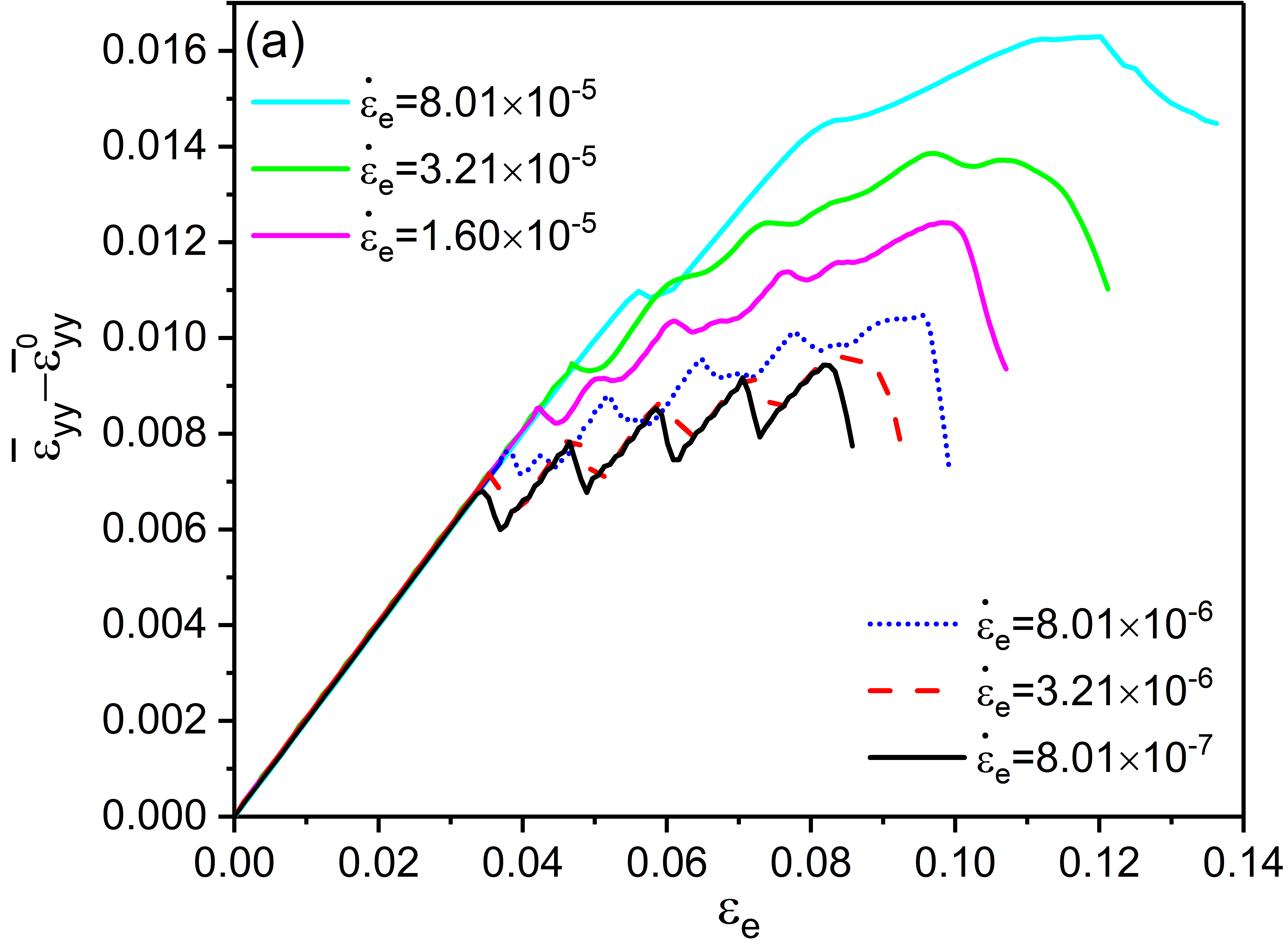
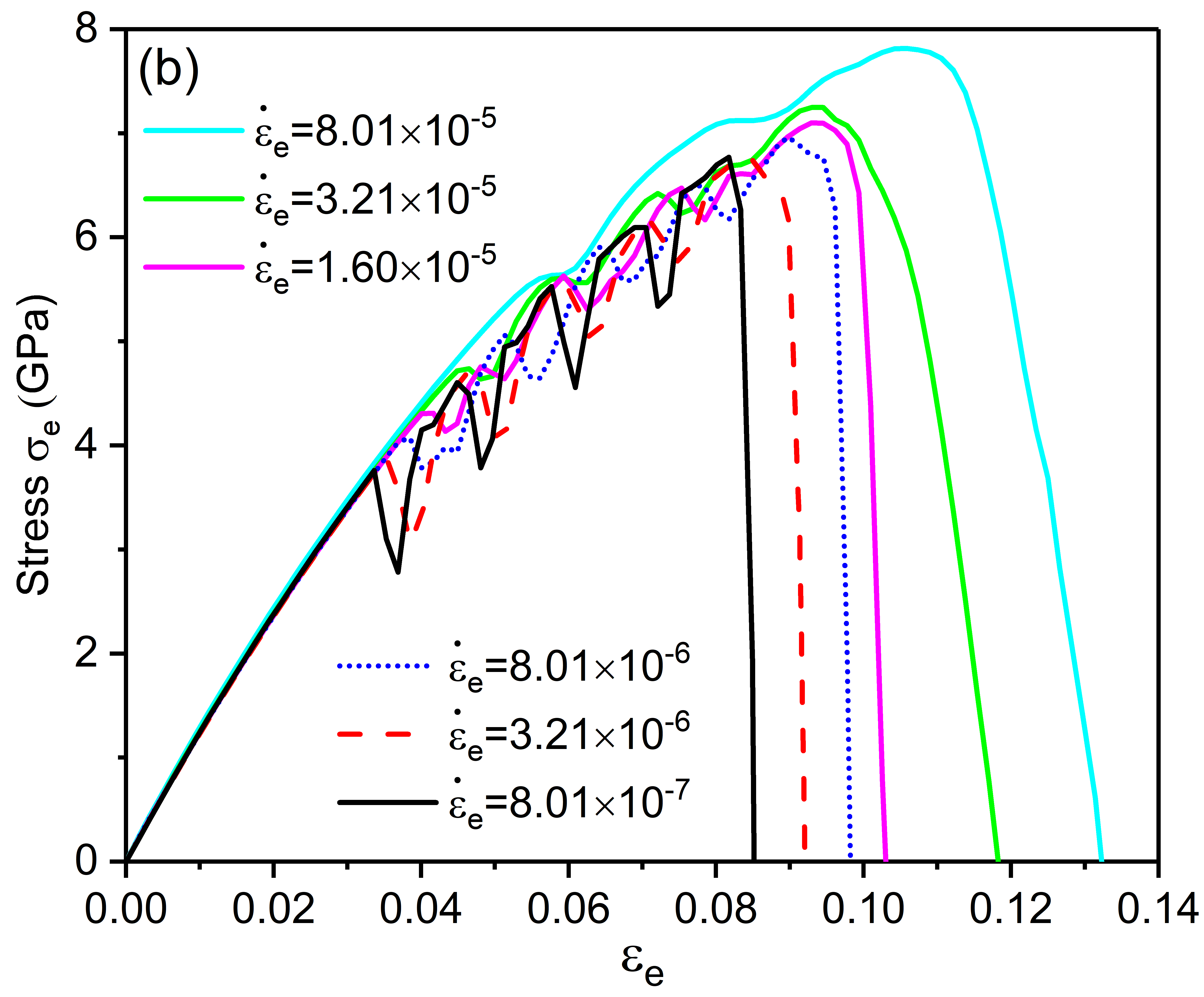
Figure 12: Effect of the applied strain rate $\dot{\varepsilon}_{e}$ on (a) the change of average local strain $\bar{\varepsilon}_{yy}-\bar{\varepsilon}_{yy}^{0}$ vs. applied strain $\varepsilon_{e}$ and (b) the stress-strain relation, for AC1 sheet at $\epsilon=-0.1$ ($T=4278$ K) that is subjected to tensile loads parallel to the GB.

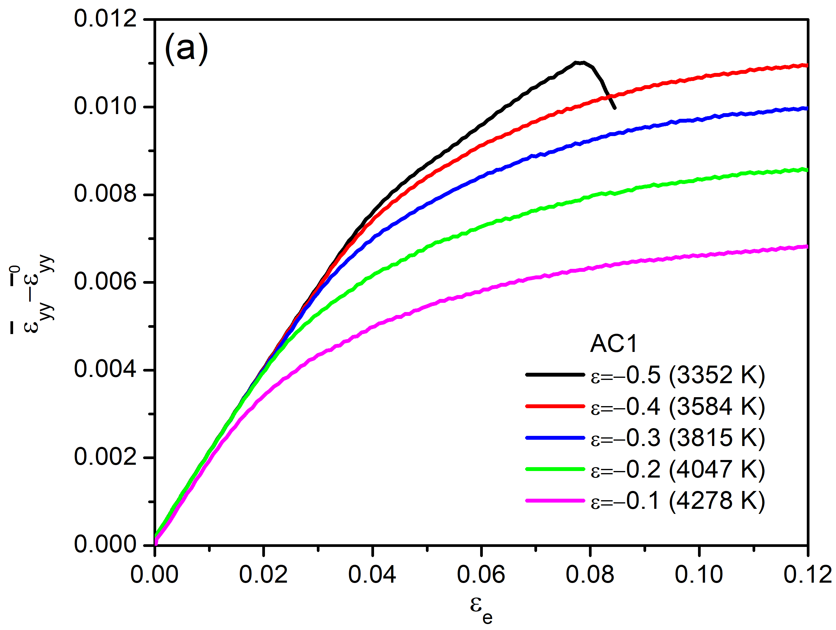
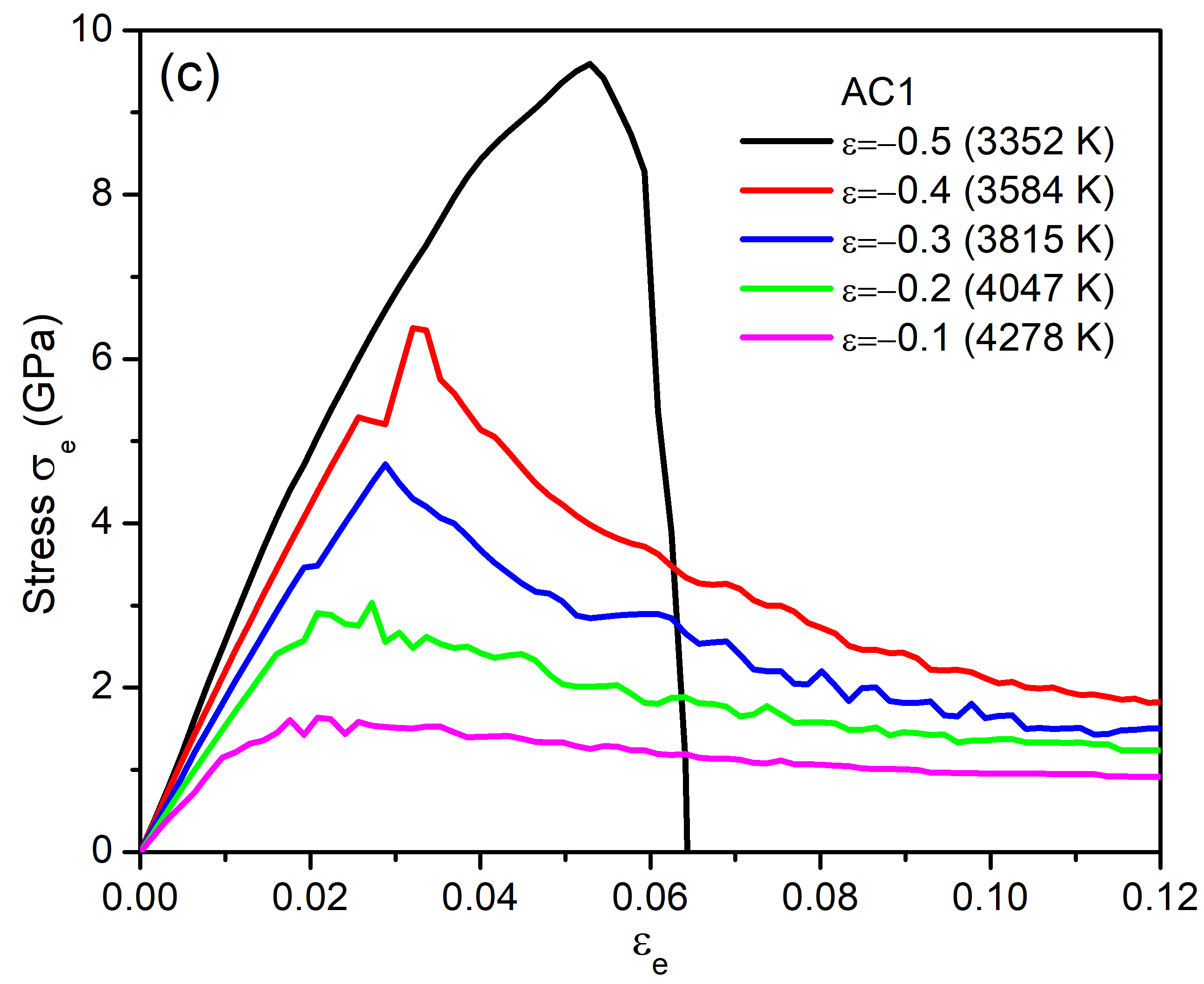
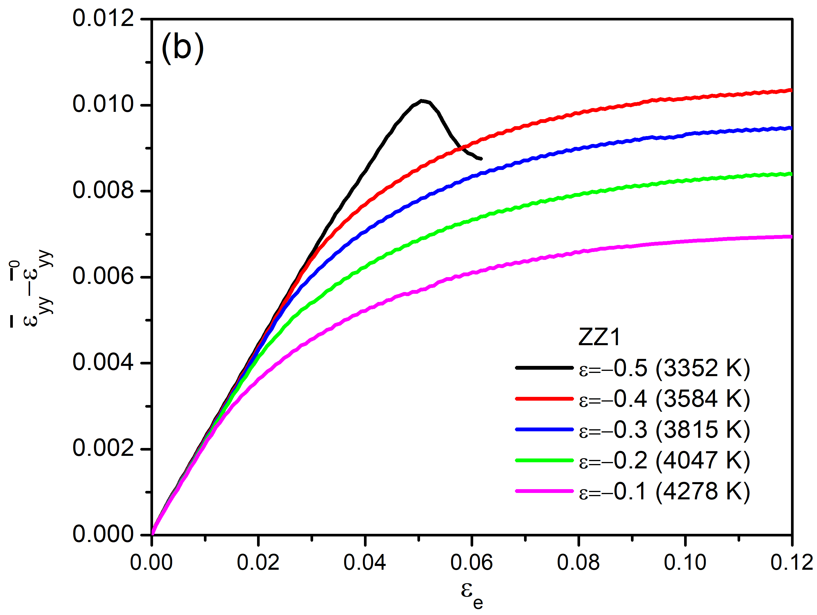
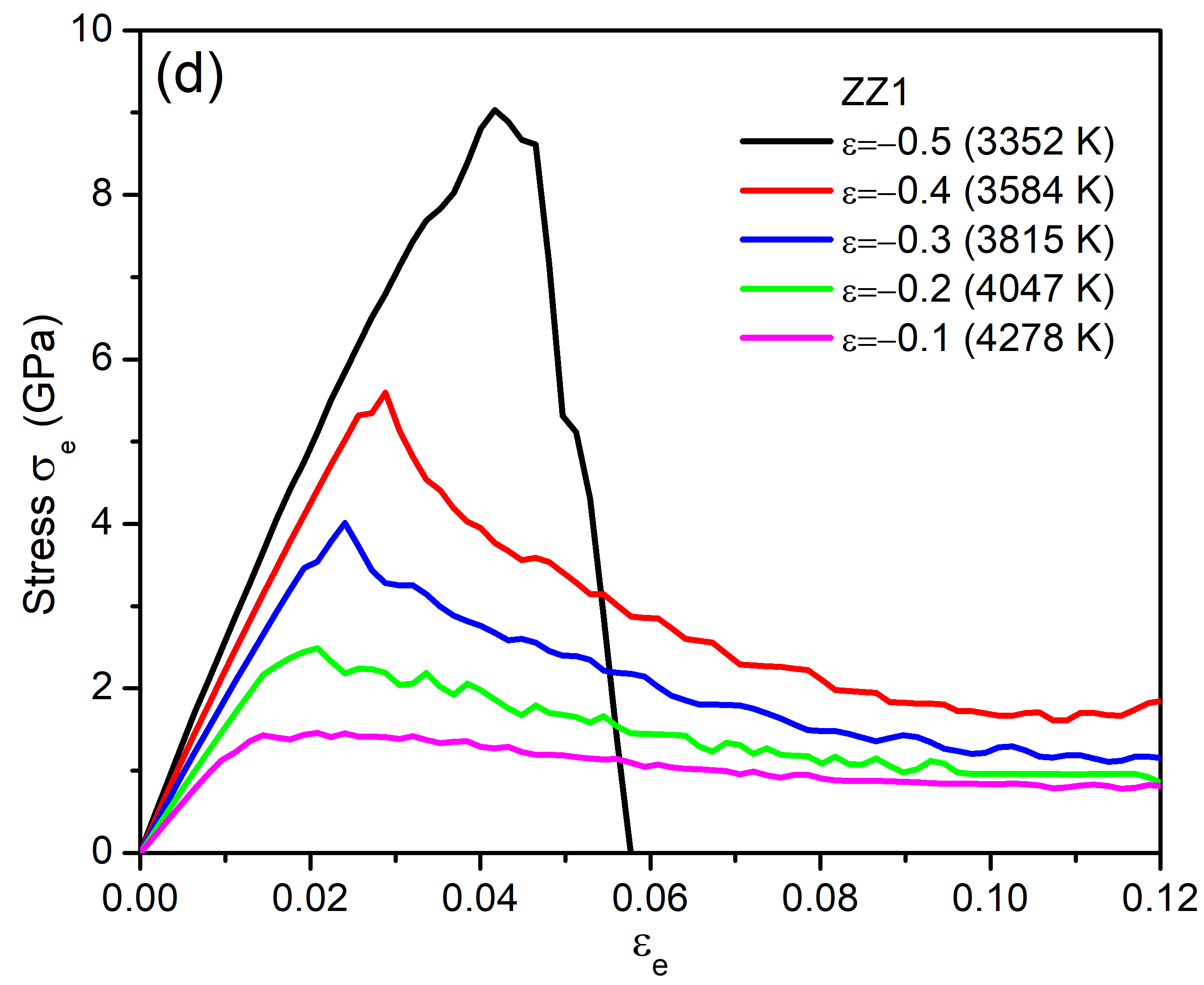
Figure 13: Change of average local strain, $\bar{\varepsilon}_{yy}-\bar{\varepsilon}_{yy}^{0}$, as a function of $\varepsilon_{e}$ for (a) AC1 and (b) ZZ1 sheets, with the direction of tensile loading perpendicular to the GBs under the strain rate $\dot{\varepsilon}_{e}=8.01\times 10^{-7}$ at different temperatures. The corresponding stress-strain curves are given in (c) and (d), respectively.

It is noted that all the above results are for the tensile loading applied parallel to the GB line. To examine the effect of external pulling direction, we conduct additional simulations for tensile loads perpendicular to the GB. The PFC system setup is similar to that of Fig. 1, other than a single GB located at $y=L_{y}/2$ in the middle of the solid region separating two misoriented grains. The GB line is aligned along the $x$ direction, perpendicular to the vertical ($y$) direction of pulling. Some sample results for low-angle GBs (AC1 and ZZ1) are given in Fig. 13, across the same temperature range as above. As seen from both the average local strain variation and the stress-strain curves, similar to the above case of parallel pulling a behavior of brittle fracture is obtained at temperature $\epsilon=-0.5$ ($T=3352$ K), while a brittle-to-ductile transition is observed at higher temperature (starting at $\epsilon=-0.4$ with $T=3584$ K in Fig. 13). However, here a different property of plastic flow is found, with much smoother and more irregular behavior compared to that shown in Figs. 10 and 11 for the parallel case. This can be attributed to different behavior of high-temperature dislocation motion before the sample failure, which is observed in our simulations to be restricted only along the GB line when the system is stretched perpendicular to the GB. In real polycrystalline samples with multiple grain orientations, any given pulling direction of the whole sample will correspond to different loading directions for different GBs, including both the parallel and perpendicular ones and mostly the scenarios in between, such that the system mechanical behavior will be the combined effect of them. In the majority of cases the GBs would not be oriented perpendicular (or nearly perpendicular) to the pulling direction, and thus the dislocation motion would not be constrained along the GB line, a scenario that is relatively closer to the case studied above with GB-parallel loading.

4 Conclusions

We have applied the phase field crystal method, which is combined with an interpolated scheme that enables fast mechanical relaxation, to examine the mechanical response of 2D graphene bicrystals across the high or ultrahigh temperature range that is beyond most of previous experiments and atomistic simulations. Small enough strain rate is used in our simulations, which is important for accessing the plastic deformation regime that is missing in atomistic studies of graphene. The systems investigated include both armchair and zigzag types of symmetric tilt grain boundaries that are subjected to uniaxial tensile loads, for low, intermediate, and high misorientation angles. For the GBs studied here, although the associated equilibrium dislocation structures and local strain distribution are mostly independent of temperature change in the absence of external stress, their mechanical behavior and deformation dynamics vary significantly when reaching high enough temperature. Even in a relatively high temperature range (around $3350$ K), results of mechanical deformation and brittle fracture that are similar to those of previous low-temperature MD simulations and experiments can be obtained, including nanovoid formation and crack initiation at the locations of GB dislocations and the subsequent crack propagation. Our PFC simulations also reveal an additional type of failure dynamics for low-angle zigzag GBs, showing as the disintegration and splitting of GB dislocation array through the migration of nanovoid-bound dislocations. An increase of temperature leads to the decrease of ultimate tensile strength and Young’s modulus for both AC and ZZ GB sheets, and more importantly, results in a transition to ductile and plastic deformation under tensile loads either parallel or perpendicular to the GB. The behavior under GB-parallel loading at high enough temperature (ranging from $3584$ K to $4278$ K for different types of GBs studied here) is characterized by jerky plasticity which is absent in all the previous studies of graphene. This jerky plastic or stick-climb-glide type behavior, as seen in both the average local strain curves and the stress-strain relation, is caused by the motion of GB dislocations (in the form of either glide-mediated climb for AC GBs or mixed motion of glide and climb for ZZ GBs) interrupted by periods of pinned and immobile defects.

The occurrence of this temperature-induced transition between brittle fracture and jerky plastic behavior depends on the type of grain boundary (armchair vs. zigzag) and the misorientation angle, particularly the type of dislocation structure and arrangement at the boundary and its local strain distribution. Microstructurally this is related to the competition between the stress-induced formation of nanovoids at the GB and the ability or degree of dislocation migration. The corresponding mechanisms are different from that of traditional brittle-to-ductile transition or the phenomenon of jerky plasticity in 3D compressed nanowires/pillars, both of which involve new dislocation nucleation that is not found here. Instead, here the mechanisms governing the jerky plastic flow are intrinsic to the 2D systems, where the migration of dislocations (locally around the GB) can be made possible by the built-up stress at high enough temperature, to overcome the constraints of pinning barriers by the lattice and the interaction of neighboring defects. Although this study is restricted to simplified systems of bicrystals and symmetric grain boundaries, the deformation mechanisms identified are generic and can be extended to the study of more complex scenarios of defected or polycrystalline graphene, and thus provide further insights into the mechanical behavior of graphene-type 2D materials particularly their mechanical performance at high temperature.

Appendix A Parameterization of PFC model for graphene

To obtain quantitative results of PFC simulation for real material systems, the PFC model described in Sec. 2.1 needs to be parameterized to match graphene. In principle the model parameterization can be conducted through the liquid-state interparticle direct correlation functions; however, the corresponding data is usually not available for most materials (except for a very limited number of material systems). Extra effort is needed to quantify and convert the parameter $\epsilon$ to real temperature $T$ and identify the corresponding conversion function $\epsilon(T)$, which would require the calculation and fitting of two-point direct correlation at various temperatures above but close to the melting point.

Here we use a different but more effective way of model parameterization for PFC graphene. From the previous PFC derivation based on classical DFT [27, 43], to lowest order the PFC temperature parameter $\epsilon$ can be approximated as

$$\epsilon=\beta(T-T_{m})/T_{m},$$ (3)

where $\beta$ is the proportional coefficient that depends on the specific material, and $T_{m}$ is the melting temperature at which $\epsilon=0$. For graphene the value of $T_{m}$ has been calculated from atomistic MC or MD simulations, but the result depends on the interaction potential and the model used, ranging from $4510$ K [9] to $5500$ K [8]. Here we choose the more recent result of $T_{m}=4510$ K which was obtained through the combination of atomistic MC simulation using LCBOPII potential and nucleation theory analysis [9]. To estimate $\beta$ for graphene we make use of a result from atomistic MC [47] and MD [46] simulations of pristine monolayer graphene, both showing a small variation of isothermal Young’s modulus $Y$ within the temperature range of $0\leq T<1500$ K followed by a decrease of $Y$ value with the increase of temperature. A similar behavior of temperature dependence is reproduced in our PFC simulations of graphene single crystals (see Fig. 14). The simulation setup is similar to that given in Ref. [44] (other than a perfect single crystal here in the solid region without double notches). We have tested different system sizes with uniaxial tensile loading along either the armchair or zigzag direction, all of which indicate a turning point around $\epsilon=-1.3$ (corresponding to $T\simeq 1500$ K) for the decrease of $Y$. Thus $\beta=1.3/(1-1500/T_{m})=1.94784053$, and from Eq. (3)

$$T=(1+\epsilon/\beta)T_{m}=T_{m}+(T_{m}-1500)\frac{\epsilon}{1.3},$$ (4)

which is used for the temperature unit conversion in this work. In the above GB study the values of $\epsilon$ are chosen from $-0.5$ to $-0.1$, corresponding to temperature $T$ ranging from $3352$ K to $4278$ K. Given the condition $T\geq 0$, from Eq. (4) we can determine the physically meaningful range of PFC temperature parameter as $\epsilon\geq-\beta=-1.94784053$ for graphene.

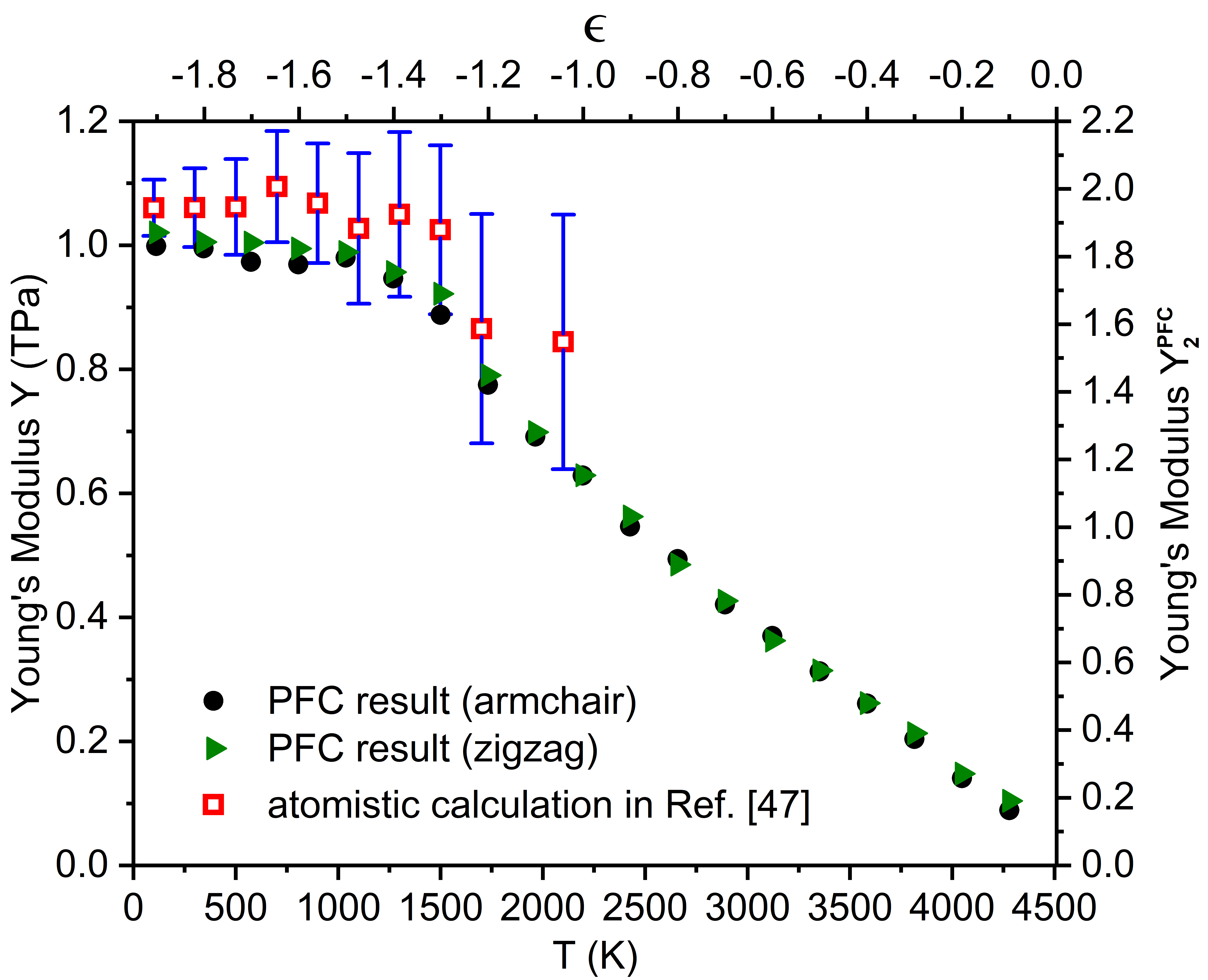
Figure 14: Young’s modulus as a function of temperature, as calculated from the PFC model for pristine graphene with uniaxial tensile loads along the armchair or zigzag direction. Both the PFC values and the corresponding real units are indicated. The data points obtained from atomistic calculations in Ref. [47] are also shown for comparison.

The PFC values for Young’s modulus and stress can also be converted to real units by noting the scaling

$$Y/Y_{2}^{\rm PFC}=\sigma/\sigma^{\rm PFC}\equiv c_{Y},$$ (5)

where $Y_{2}^{\rm PFC}$ is the 2D PFC Young’s modulus and $\sigma^{\rm PFC}$ is the dimensionless stress calculated in PFC. Knowing that the lowest temperature used in our single-crystal PFC simulation is at $\epsilon=-1.9$ with $T\simeq 111$ K, and the corresponding PFC Young’s modulus $Y_{2}^{\rm PFC}(\epsilon=-1.9)=1.83126$ (for the armchair direction; see Fig. 14) can be matched to the low-temperature value of $Y=1$ TPa measured in experiments [2], we have the conversion factor $c_{Y}=1/1.83126$ TPa, which is applied to all our results of mechanical calculations.

A sample result of our PFC calculation for Young’s modulus of pristine graphene is presented in Fig. 14, with system size $2048\Delta x\times 2048\Delta y$ (i.e., $54.5$ nm $\times$ $54.5$ nm) and the initial active solid zone of size $1648\Delta x\times 1648\Delta y$ (i.e., $43.9$ nm $\times$ $43.9$ nm). Both the dimensionless PFC values and the corresponding real-unit converted values are shown in the figure, as well as the data from atomistic MC calculations in Ref. [47] which used the same LCBOPII potential as that of Ref. [9] giving $T_{m}=4510$ K. Note that overall the MC data points appear to be shifted upward (i.e., of larger value) compared to the PFC ones, which is due to the use of $Y=1$ TPa at low $T$ in our unit scaling based on the experimental result [2], instead of $1.06$ TPa calculated in Ref. [47].

The conversion for length scale can be determined by [30]

$$l/l^{\rm PFC}=a_{0}/a_{0}^{\rm PFC}\simeq(2.46~{}\textrm{\AA})/(4\pi/\sqrt{3})=0.3391~{}\textrm{\AA},$$ (6)

based on the PFC lattice spacing $a_{0}^{\rm PFC}\simeq 4\pi/\sqrt{3}$ and the graphene lattice constant $a_{0}=2.46$ Å. Thus in the above PFC simulations of GBs the system size used, $512\Delta x\times 2048\Delta y$, corresponds to $13.6$ nm $\times$ $54.5$ nm, while its initial active solid zone is of size $512\Delta x\times 1248\Delta y$, i.e., $13.6$ nm $\times$ $33.2$ nm. In addition, the time scale of PFC has been identified (see Ref. [44]), i.e.,

$$t/t^{\rm PFC}=\left(a_{0}/a_{0}^{\rm PFC}\right)^{2}(D^{\rm PFC}/D),$$ (7)

where $D^{\rm PFC}$ is the dimensionless vacancy diffusion constant in PFC [26] and $D$ is the corresponding value of the real material (i.e., graphene). This clearly indicates the diffusive nature of the characteristic timescales for evolution and dynamics of PFC.

For completeness we summarize in Table 1 a list of six GBs examined in this work, including the corresponding type of dislocations at the GB and the grain boundary energies calculated from the PFC model. Values of these GB energies are adapted from Ref. [38] which also presents the results across the full range of misorientation angles for various versions of PFC models as well as MD and quantum DFT calculations.

Table 1: Summary of the six symmetric tilt grain boundaries studied in this work, including the type of dislocations at the boundary and the grain boundary energy which has been calculated in Ref. [38] using the same PFC model as that of Sec. 2.1.

	$\theta$	Dislocation type	GB energy (eV/nm) [38]
AC1	$7.34^{\circ}$	$(1,0)$	4.2450
AC2	$13.17^{\circ}$	$(1,0)$	5.6655
AC3	$21.79^{\circ}$	$(1,0)$	6.6075
ZZ1	$8.61^{\circ}$	$(1,0),(0,1)$	5.2678
ZZ2	$13.17^{\circ}$	$(1,0),(0,1)$	6.3764
ZZ3	$23.49^{\circ}$	$(1,0)+(0,1)+(1,0)$,	7.4849
		$(0,1)+(1,0)+(0,1)$

Appendix B Numerical scheme and low-temperature GB results

In this work we use a pseudospectral algorithm to solve the PFC dynamic Eq. (2). The equation can be rewritten as $\partial\phi/\partial t=\tilde{L}\phi+f$, where $\tilde{L}$ represents a linear operator given by $\tilde{L}=\nabla^{2}[\epsilon+(1+\nabla^{2})^{2}]$, and the nonlinear terms are denoted as $f=\nabla^{2}(\tau\phi^{2}+\phi^{3})$. This is a sixth-order nonlinear partial differential equation. If transforming the equation to Fourier space, with $\tilde{\phi}_{k}=\int d\vec{r}\phi(\vec{r})e^{-i\vec{k}\cdot\vec{r}}$ the Fourier transform of the density field $\phi$, the PFC equation can be simplified as

$$\frac{\partial\tilde{\phi}_{k}}{\partial t}=\tilde{L}_{k}\tilde{\phi}_{k}+\tilde{f}_{k},$$ (8)

where $\tilde{L}_{k}=-(\epsilon+1)k^{2}+2k^{4}-k^{6}$ and $\tilde{f}_{k}=-k^{2}\int d\vec{r}(\tau\phi^{2}+\phi^{3})e^{-i\vec{k}\cdot\vec{r}}$ represent the Fourier transforms of the linear operator and the nonlinear terms, respectively, and $\vec{k}$ is the wave vector. Following the exponential propagation scheme for the linear term and the predictor-corrector method for the nonlinear terms as described in Ref. [60], we have

$$\tilde{\phi}_{k}(t+\Delta t)= e^{\tilde{L}_{k}\Delta t}\tilde{\phi}_{k}(t)+\frac{e^{\tilde{L}_{k}\Delta t}-1}{\tilde{L}_{k}}\tilde{f}_{k}(t)$$ (9)

$$+\left(e^{\tilde{L}_{k}\Delta t}-\tilde{L}_{k}\Delta t-1\right)\frac{\tilde{f}_{k}(t+\Delta t)-\tilde{f}_{k}(t)}{{\tilde{L}_{k}}^{2}\Delta t},$$

when $\tilde{L}_{k}\neq 0$, and

$$\tilde{\phi}_{k}(t+\Delta t)=\tilde{\phi}_{k}(t)+\tilde{f}_{k}(t)\Delta t+\frac{1}{2}\Delta t\left[\tilde{f}_{k}(t+\Delta t)-\tilde{f}_{k}(t)\right],$$ (10)

when $\tilde{L}_{k}=0$. This implicit scheme can be implemented by an iterative procedure of predictor-corrector steps, although we usually need only one iteration of the corrector step for numerical convergence and accuracy.

In addition to the high-temperature simulations given above, we have conducted mechanical calculations for both AC and ZZ GBs at a low temperature of $\epsilon=-1.9$ ($T=111$ K), to compare with previous atomistic simulations and experimental observation. Other model parameters and system setup are the same as those in Secs. 3.2 and 3.3 (except for a smaller time step $\Delta t=0.1$). Some results are presented in Fig. 15 for tensile loads parallel to the GB, including the stress-strain curves and some snapshots of brittle fracture and crack propagation into the grain interior (but not along the GB), which are consistent with those of previous low-temperature MD simulations [18] and experiments [6, 7] of graphene. Note that the notation of armchair vs. zigzag GB used here is opposite to that in Ref. [18]; also the PFC stress values obtained here for ZZ GBs (Fig. 15(b)) are noticeably lower than the MD results, which can be attributed to the fact that the dislocation structure and arrangement of ZZ GBs that form naturally from PFC dynamic evolution of density field are more disperse than those set up manually or by a predetermined way in MD simulations and are of lower energy (see also the discussion at the end of Sec. 3.2).

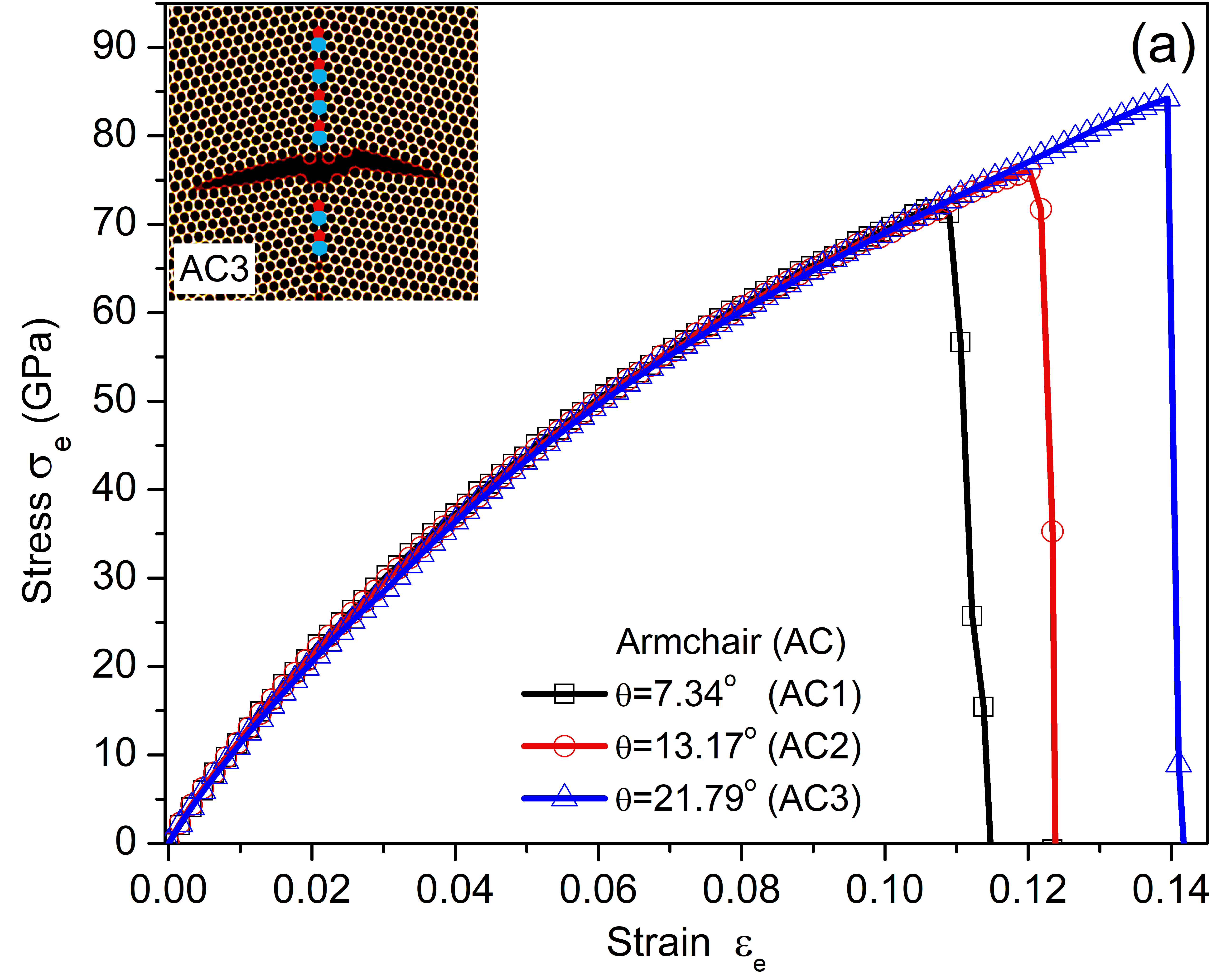
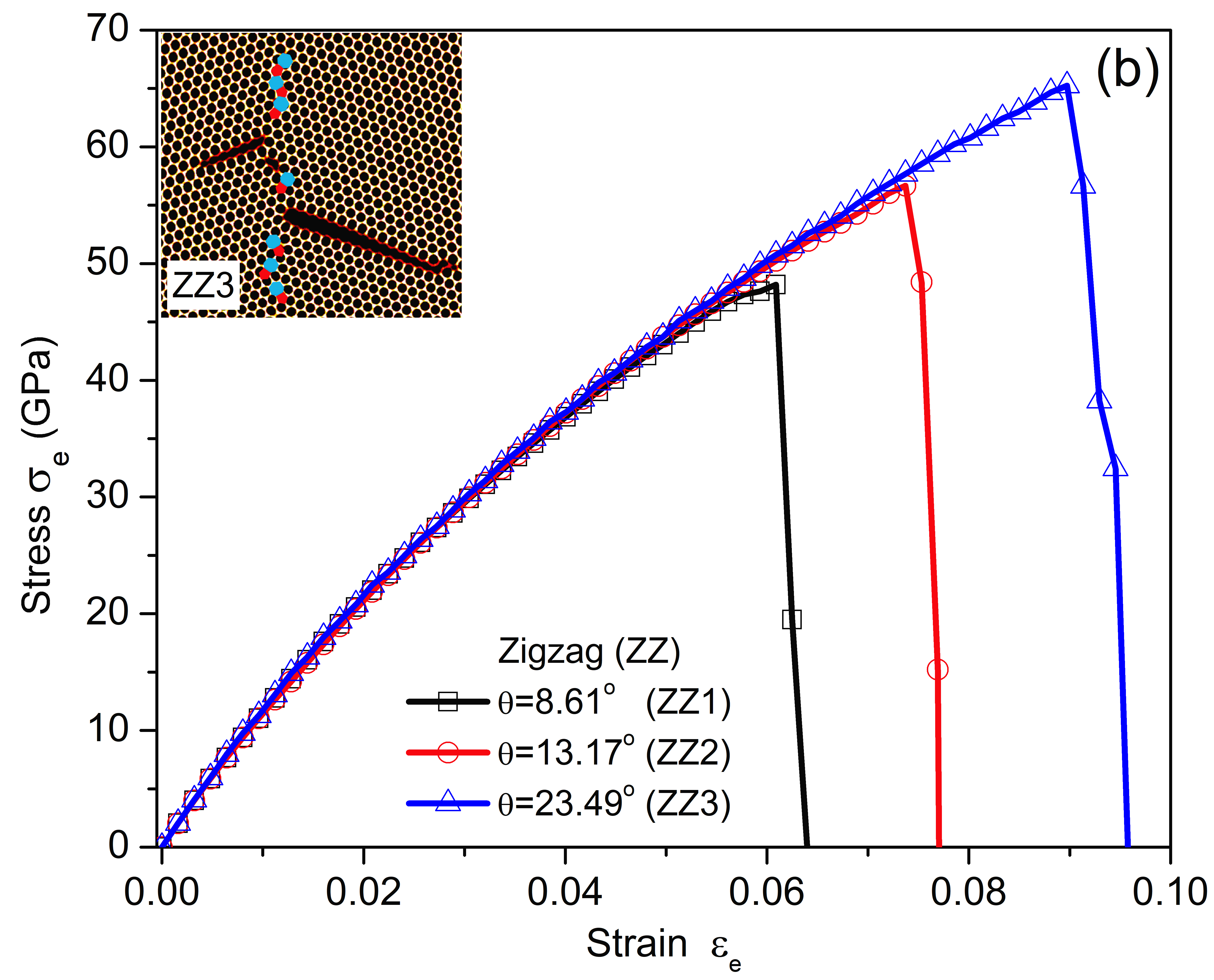
Figure 15: Stress-strain curves for (a) AC and (b) ZZ sheets at $\epsilon=-1.9$ ($T=111$ K) under uniaxial tension applied parallel to the GBs. Sample atomic structures at the stage of brittle fracture and cracking are also shown in the insets of (a) for AC3 at $\varepsilon_{e}=14.26\%$ and (b) for ZZ3 at $\varepsilon_{e}=9.46\%$.

References

- [1] A. K. Geim, Graphene: Status and prospects, Science 324 (2009) 1530–1534.
- [2] C. Lee, X. Wei, J. W. Kysar, J. Hone, Measurement of the elastic properties and intrinsic strength of monolayer graphene, Science 321 (2008) 385–388.
- [3] P. Y. Huang, C. S. Ruiz-Vargas, A. M. van der Zande, W. S. Whitney, M. P. Levendorf, J. W. Kevek, S. Garg, J. S. Alden, C. J. Hustedt, Y. Zhu, J. Park, P. L. McEuen, D. A. Muller, Grains and grain boundaries in single-layer graphene atomic patchwork quilts, Nature 469 (2011) 389–392.
- [4] G.-H. Lee, R. C. Cooper, S. J. An, S. Lee, A. van der Zande, N. Petrone, A. G. Hammerberg, C. Lee, B. Crawford, W. Oliver, J. W. Kysar, J. Hone, High-strength chemical-vapor-deposited graphene and grain boundaries, Science 340 (2013) 1073–1076.
- [5] C. S. Ruiz-Vargas, H. L. Zhuang, P. Y. Huang, A. M. van der Zande, S. Garg, P. L. McEuen, D. A. Muller, R. G. Hennig, J. Park, Softened elastic response and unzipping in chemical vapor deposition graphene membranes, Nano Lett. 11 (6) (2011) 2259–2263.
- [6] K. Kim, V. I. Artyukhov, W. Regan, Y. Liu, M. F. Crommie, B. I. Yakobson, A. Zettl, Ripping graphene: Preferred directions, Nano Lett. 12 (1) (2012) 293–297.
- [7] H. I. Rasool, C. Ophus, W. S. Klug, A. Zettl, J. K. Gimzewski, Measurement of the intrinsic strength of crystalline and polycrystalline graphene, Nat. Commun. 4 (2013) 2811.
- [8] S. K. Singh, M. Neek-Amal, F. M. Peeters, Melting of graphene clusters, Phys. Rev. B 87 (2013) 134103.
- [9] J. H. Los, K. V. Zakharchenko, M. I. Katsnelson, A. Fasolino, Melting temperature of graphene, Phys. Rev. B 91 (2015) 045415.
- [10] A. S. Mayorov, R. V. Gorbachev, S. V. Morozov, L. Britnell, R. Jalil, L. A. Ponomarenko, P. Blake, K. S. Novoselov, K. Watanabe, T. Taniguchi, A. K. Geim, Micrometer-scale ballistic transport in encapsulated graphene at room temperature, Nano Lett. 11 (6) (2011) 2396–2399.
- [11] D. A. Dikin, S. Stankovich, E. J. Zimney, R. D. Piner, G. H. B. Dommett, G. Evmenenko, S. T. Nguyen, R. S. Ruoff, Preparation and characterization of graphene oxide paper, Nature 448 (2007) 457–460.
- [12] E. Sest, G. Drazic, B. Genorio, I. Jerman, Graphene nanoplatelets as an anticorrosion additive for solar absorber coatings, Sol. Energy Mater. Sol. Cells 176 (2018) 19–29.
- [13] E. Sani, J. P. Vallejo, D. Cabaleiro, L. Lugo, Functionalized graphene nanoplatelet-nanofluids for solar thermal collectors, Sol. Energy Mater. Sol. Cells 185 (2018) 205–209.
- [14] K. Abinaya, S. Karthikaikumar, K. Sudha, S. Sundharamurthi, A. Elangovan, P. Kalimuthu, Synergistic effect of 9-(pyrrolidin-1-yl)perylene-3,4-dicarboximide functionalization of amino graphene on photocatalytic hydrogen generation, Sol. Energy Mater. Sol. Cells 185 (2018) 431–438.
- [15] Y. D. Kim, H. Kim, Y. Cho, J. H. Ryoo, C.-H. Park, P. Kim, Y. S. Kim, S. Lee, Y. Li, S.-N. Park, Y. S. Yoo, D. Yoon, V. E. Dorgan, E. Pop, T. F. Heinz, J. Hone, S.-H. Chun, H. Cheong, S. W. Lee, M.-H. Bae, Y. D. Park, Bright visible light emission from graphene, Nat. Nanotechnol. 10 (2015) 676–681.
- [16] See Wendelstein 7-X website https://www.ipp.mpg.de/4555488/op_1_2.
- [17] G. Xin, T. Yao, H. Sun, S. M. Scott, D. Shao, G. Wang, J. Lian, Highly thermally conductive and mechanically strong graphene fibers, Science 349 (2015) 1083–1087.
- [18] R. Grantab, V. B. Shenoy, R. S. Ruoff, Anomalous strength characteristics of tilt grain boundaries in graphene, Science 330 (2010) 946–948.
- [19] Y. Wei, J. Wu, H. Yin, X. Shi, R. Yang, M. Dresselhaus, The nature of strength enhancement and weakening by pentagon-heptagon defects in graphene, Nat. Mater. 11 (2012) 759–763.
- [20] T.-H. Liu, C.-W. Pao, C.-C. Chang, Effects of dislocation densities and distributions on graphene grain boundary failure strengths from atomistic simulations, Carbon 50 (10) (2012) 3465–3472.
- [21] J. Wu, Y. Wei, Grain misorientation and grain-boundary rotation dependent mechanical properties in polycrystalline graphene, J. Mech. Phys. Solids 61 (6) (2013) 1421–1432.
- [22] L. Yi, Z. Yin, Y. Zhang, T. Chang, A theoretical evaluation of the temperature and strain-rate dependent fracture strength of tilt grain boundaries in graphene, Carbon 51 (2013) 373–380.
- [23] M. Q. Chen, S. S. Quek, Z. D. Sha, C. H. Chiu, Q. X. Pei, Y. W. Zhang, Effects of grain size, temperature and strain rate on the mechanical properties of polycrystalline graphene – a molecular dynamics study, Carbon 85 (2015) 135–146.
- [24] Z. Yang, Y. Huang, F. Ma, Y. Sun, K. Xu, P. K. Chu, Temperature and strain-rate effects on the deformation behaviors of nano-crystalline graphene sheets, Euro. Phys. J. B 88 (5) (2015) 135.
- [25] K. R. Elder, M. Katakowski, M. Haataja, M. Grant, Modeling elasticity in crystal growth, Phys. Rev. Lett. 88 (2002) 245701.
- [26] K. R. Elder, M. Grant, Modeling elastic and plastic deformations in nonequilibrium processing using phase field crystals, Phys. Rev. E 70 (2004) 051605.
- [27] K. R. Elder, N. Provatas, J. Berry, P. Stefanovic, M. Grant, Phase field crystal modeling and classical density functional theory of freezing, Phys. Rev. B 75 (2007) 064107.
- [28] P. Stefanovic, M. Haataja, N. Provatas, Phase-field crystals with elastic interactions, Phys. Rev. Lett. 96 (2006) 225504.
- [29] S. K. Mkhonta, K. R. Elder, Z.-F. Huang, Exploring the complex world of two-dimensional ordering with three modes, Phys. Rev. Lett. 111 (2013) 035501.
- [30] D. Taha, S. K. Mkhonta, K. R. Elder, Z.-F. Huang, Grain boundary structures and collective dynamics of inversion domains in binary two-dimensional materials, Phys. Rev. Lett. 118 (2017) 255501.
- [31] P. Stefanovic, M. Haataja, N. Provatas, Phase field crystal study of deformation and plasticity in nanocrystalline materials, Phys. Rev. E 80 (2009) 046107.
- [32] M. Salvalaglio, R. Backofen, K. R. Elder, A. Voigt, Defects at grain boundaries: A coarse-grained, three-dimensional description by the amplitude expansion of the phase-field crystal model, Phys. Rev. Mater. 2 (2018) 053804.
- [33] A. Skaugen, L. Angheluta, J. Viñals, Separation of elastic and plastic timescales in a phase field crystal model, Phys. Rev. Lett. 121 (2018) 255501.
- [34] C. Guo, J. Wang, J. Li, Z. Wang, Y. Huang, J. Gu, X. Lin, Coupling eutectic nucleation mechanism investigated by phase field crystal model, Acta Mater. 145 (2018) 175–185.
- [35] W. Zhou, J. Wang, Z. Wang, Q. Zhang, C. Guo, J. Li, Y. Guo, Size effects of shear deformation response for nano-single crystals examined by the phase-field-crystal model, Comput. Mater. Sci. 127 (2017) 121–127.
- [36] Y. Gao, L. Huang, Q. Deng, W. Zhou, Z. Luo, K. Lin, Phase field crystal simulation of dislocation configuration evolution in dynamic recovery in two dimensions, Acta Mater. 117 (2016) 238–251.
- [37] Y. Gao, Z. Luo, L. Huang, H. Mao, C. Huang, K. Lin, Phase field crystal study of nano-crack growth and branch in materials, Modelling Simul. Mater. Sci. Eng. 24 (5) (2016) 055010.
- [38] P. Hirvonen, M. M. Ervasti, Z. Fan, M. Jalalvand, M. Seymour, S. M. Vaez Allaei, N. Provatas, A. Harju, K. R. Elder, T. Ala-Nissila, Multiscale modeling of polycrystalline graphene: A comparison of structure and defect energies of realistic samples from phase field crystal models, Phys. Rev. B 94 (2016) 035414.
- [39] P. Hirvonen, Z. Fan, M. M. Ervasti, A. Harju, K. R. Elder, T. Ala-Nissila, Energetics and structure of grain boundary triple junctions in graphene, Sci. Rep. 7 (1) (2017) 4754.
- [40] M. Smirman, D. Taha, A. K. Singh, Z.-F. Huang, K. R. Elder, Influence of misorientation on graphene moiré patterns, Phys. Rev. B 95 (2017) 085407.
- [41] J. Li, B. Ni, T. Zhang, H. Gao, Phase field crystal modeling of grain boundary structures and growth in polycrystalline graphene, J. Mech. Phys. Solids 120 (2018) 36–48.
- [42] M. Seymour, N. Provatas, Structural phase field crystal approach for modeling graphene and other two-dimensional structures, Phys. Rev. B 93 (2016) 035447.
- [43] Z.-F. Huang, K. R. Elder, N. Provatas, Phase-field-crystal dynamics for binary systems: Derivation from dynamical density functional theory, amplitude equation formalism, and applications to alloy heterostructures, Phys. Rev. E 82 (2010) 021605.
- [44] W. Zhou, J. Wang, Z. Wang, Z.-F. Huang, Mechanical relaxation and fracture of phase field crystals, Phys. Rev. E 99 (2019) 013302.
- [45] H. Zhao, K. Min, N. R. Aluru, Size and chirality dependent elastic properties of graphene nanoribbons under uniaxial tension, Nano Lett. 9 (2009) 3012–3015.
- [46] H. Zhao, N. R. Aluru, Temperature and strain-rate dependent fracture strength of graphene, J. Appl. Phys. 108 (6) (2010) 064321.
- [47] K. V. Zakharchenko, M. I. Katsnelson, A. Fasolino, Finite temperature lattice properties of graphene beyond the quasiharmonic approximation, Phys. Rev. Lett. 102 (2009) 046808.
- [48] F. Liu, P. Ming, J. Li, Ab initio calculation of ideal strength and phonon instability of graphene under tension, Phys. Rev. B 76 (2007) 064120.
- [49] Z. Wang, J. Li, Y. Guo, S. Tang, J. Wang, Unique visualization of multiply oriented lattice structures using a continuous wavelet transform, Comput. Phys. Commun. 184 (11) (2013) 2489–2493.
- [50] O. V. Yazyev, S. G. Louie, Topological defects in graphene: Dislocations and grain boundaries, Phys. Rev. B 81 (2010) 195420.
- [51] Y. Liu, B. I. Yakobson, Cones, pringles, and grain boundary landscapes in graphene topology, Nano Lett. 10 (6) (2010) 2178–2183.
- [52] M. J. Hytch, J.-L. Putaux, J.-M. Penisson, Measurement of the displacement field of dislocations to 0.03 Å by electron microscopy, Nature 423 (2003) 270.
- [53] Y. Guo, J. Wang, Z. Wang, J. Li, S. Tang, F. Liu, Y. Zhou, Strain mapping in nanocrystalline grains simulated by phase field crystal model, Philos. Mag. 95 (9) (2015) 973–984.
- [54] T.-H. Liu, G. Gajewski, C.-W. Pao, C.-C. Chang, Structure, energy, and structural transformations of graphene grain boundaries from atomistic simulations, Carbon 49 (7) (2011) 2306 – 2317.
- [55] B. I. Yakobson, F. Ding, Observational geology of graphene, at the nanoscale, ACS Nano 5 (3) (2011) 1569–1574.
- [56] A. Shekhawat, C. Ophus, R. O. Ritchie, A generalized read-shockley model and large scale simulations for the energy and structure of graphene grain boundaries, RSC Adv. 6 (2016) 44489–44497.
- [57] J. Zhang, J. Zhao, Structures and electronic properties of symmetric and nonsymmetric graphene grain boundaries, Carbon 55 (2013) 151–159.
- [58] G. J. Tucker, Z. H. Aitken, J. R. Greer, C. R. Weinberger, The mechanical behavior and deformation of bicrystalline nanowires, Modelling Simul. Mater. Sci. Eng. 21 (2013) 015004.
- [59] P. J. Imrich, C. Kirchlechner, C. Motz, G. Dehm, Differences in deformation behavior of bicrystalline Cu micropillars containing a twin boundary or a large-angle grain boundary, Acta Mater. 73 (2014) 240–250.
- [60] M. C. Cross, D. Meiron, Y. Tu, Chaotic domains: A numerical investigation, Chaos 4 (4) (1994) 607–619.