Abstract

Objective

Proton computed tomography (CT) is similar to x-ray CT but relies on protons rather than photons to form an image. In its most common operation mode, the measured quantity is the amount of energy that a proton has lost while traversing the imaged object from which a relative stopping power map can be obtained via tomographic reconstruction. To this end, a calorimeter which measures the energy deposited by protons downstream of the scanned object has been studied or implemented as energy detector in several proton CT prototypes. An alternative method is to measure the proton’s residual velocity and thus its kinetic energy via the time of flight (TOF) between at least two sensor planes. In this work, we study the precision, i.e. image noise, which can be expected from TOF proton CT systems.

Approach

We rely on physics models on the one hand and statistical models of the relevant uncertainties on the other to derive closed form expressions for the noise in projection images. The TOF measurement error scales with the distance between the TOF sensor planes and is reported as velocity error in ps/m. We use variance reconstruction to obtain noise maps of a water cylinder phantom given the scanner characteristics and additionally reconstruct noise maps for a calorimeter-based proton CT system as reference.

Main results

We find that TOF proton CT with 30 ps/m velocity error reaches similar image noise as a calorimeter-based proton CT system with 1% energy error (1 sigma error). A TOF proton CT system with a 50 ps/m velocity error produces slightly less noise than a 2% calorimeter system. Noise in a reconstructed TOF proton CT image is spatially inhomogeneous with a marked increase towards the object periphery.

Significance

This systematic study of image noise in TOF proton CT can serve as a guide for future developments of this alternative solution for estimating the residual energy of protons after the scanned object.

1 Introduction

Proton computed tomography (CT) is a transmission imaging modality similar to x-ray CT which uses protons instead of x-ray for image acquisition [17]. While x-ray CT relies on attenuation, proton CT is typically operated in energy-loss mode where the amount of energy lost by a proton while traversing the imaged object depends on the water equivalent amount of material. The reconstructed quantity in this case is the so-called relative stopping power (RSP), i.e. the proton stopping power relative to that of water. A proton CT scanner typically includes a suitable detector to measure the protons’ residual energy, i.e. after traversing the scanned object, from which, together with the beam energy, the energy loss can be obtained. Proton CT scanner prototypes proposed and developed so far rely either on a calorimeter, e.g. a scintillator, to measure the energy deposited by a proton therein [8, 16, 11] or a range telescope [34, 3, 23]. An alternative measurement principle determines the proton’s time of flight (TOF) between two or more sensor planes from which the velocity and thus the kinetic energy can be calculated. Although [39] reported on developments of a TOF proton radiography system and presented some first experimental results, TOF proton CT has overall not been fully explored yet. [36] recently investigated the feasibility of a TOF proton CT system using low gain avalanche detectors [22] based on Monte Carlo simulations. They studied RSP accuracy and RSP precision with a focus on the detector hardware and possible calibration procedures. [38] discusses TOF as an alternative measurement principle in helium CT and analyses aspects related to RSP resolution. RSP precision has previously been investigated for energy-loss proton CT based on calorimeter detectors [33, 9, 27, 13] as well as for other proton CT modalities which do not require residual energy measurements [26, 19, 7].

This work provides a concise and systematic study of RSP precision in TOF proton CT, which manifests itself as image noise, based on physics models and statistics. As sources of uncertainty, we consider the TOF measurement error, energy straggling inside the imaged object, as well as the proton beam’s energy spread. We analyse noise on a projection level and also reconstruct noise images [40, 27] of a water cylinder to assess the RSP precision depending on the location in the reconstructed image. In this context, we consider only direct reconstruction algorithms [18] and distance driven binning backprojection in particular [29].

The contribution of this work is to provide the necessary tools to quickly model RSP in a TOF proton CT system and to derive figures of merit of the achievable RSP precision given the system’s characteristics and the properties of the imaged object, similar to the pioneering work of [33] for energy-loss proton CT.

2 Materials and Methods

2.1 Statistical aspects of TOF proton CT

With noise in the proton CT images, we intend the variation of RSP value which one would observe in each pixel in repeated acquisitions of the same object, as described e.g. in [40]. Image noise is therefore synonymous to the RSP precision or RSP resolution. The RSP value is obtained via tomographic image reconstruction which takes a series of projections as input. The projections contain water equivalent path length (WEPL) values which are in turn converted from the proton’s energy-loss, e.g. via a look-up table. Therefore, statistical errors in the energy-loss are propagated into the reconstructed RSP value.

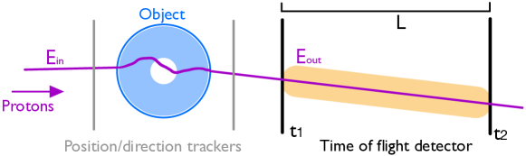
Figure 1: Schematic illustration of a TOF proton CT scanner. The residual energy is deduced from the time $t_{2}-t_{1}$ which the proton needs to travel from one sensor plane to the other. The trackers which measure the proton’s position and direction are shown for completeness, although not directly relevant for this work.

We consider a TOF proton CT set-up made of a TOF device consisting of two sensor planes downstream of the scanned object. A proton CT scanner typically also includes tracking devices upstream and downstream of the scanned object, but they are not directly relevant to this work. A sketch is shown in figure 1. We assume that the TOF device records the time needed to travel from one sensor plane to the other, from which the proton’s kinetic energy downstream of the imaged object can be determined. The initial proton energy is taken as the beam energy provided by the accelerator. We do not attempt to simulate any specific TOF proton CT prototype.

We consider three contributions to image noise, namely the error of the TOF measurement, energy straggling experienced by the protons, and the energy spread of the proton beam. We denote with $E_{\mathrm{in}}$ and $E_{\mathrm{out}}$ the proton’s energy upstream and downstream of the imaged object, respectively. We disregard nuclear interactions and assume that protons recorded by the proton CT system have only undergone electromagnetic interactions. In practice, most protons which have undergone nuclear interactions are filtered out from the data prior to image reconstruction [17, 32]. We treat energy straggling and the time measurement error of the TOF device within the Gaussian approximation.

$E_{\mathrm{out}}$ is determined from the time of flight between the TOF sensor planes, $t_{2}-t_{1}$, as

$$E_{\mathrm{out}}=\frac{m_{p}c^{2}}{\sqrt{1-(v/c)^{2}}}-m_{p}c^{2}\quad\mathrm{with}\quad v=\frac{L}{t_{2}-t_{1}},$$ (1)

where $L$ is the distance between the TOF sensor planes and $m_{p}=938$ MeV/c² is the proton mass. Energy loss in 1 mm of silicon or 1 m of air is on the order of 0.5 MeV for protons with an energy between 100 MeV and 200 MeV [6]. We therefore neglect energy loss in the trackers, the TOF sensors, and the surrounding air. By first order error propagation one has

$$\sigma_{E_{\mathrm{out}},\mathrm{TOF}}(E_{\mathrm{out}})=\left(\left|\frac{\mathop{}\!\mathrm{d}E}{\mathop{}\!\mathrm{d}t_{1}}\right|^{2}\sigma^{2}_{t_{1}}+\left|\frac{\mathop{}\!\mathrm{d}E}{\mathop{}\!\mathrm{d}t_{2}}\right|^{2}\sigma^{2}_{t_{2}}\right)^{1/2}=\frac{1}{m^{2}_{p}c^{3}}(E_{\mathrm{out}}^{2}+2m_{p}c^{2}E_{\mathrm{out}})^{3/2}\;\frac{\sigma_{t}}{L},$$ (2)

where $\sigma_{t}^{2}=\sigma_{t_{1}}^{2}+\sigma_{t_{2}}^{2}$ is the TOF measurement error stemming from the time resolution of the two sensors. Note that the error on $E_{\mathrm{out}}$ directly scales with $L$ so that a greater spacing between the TOF planes will reduce the energy measurement error. Throughout this work, we report the velocity error $\sigma_{t}/L$ in units of ps/m, rather than $\sigma_{t}$ alone.

Energy straggling of protons inside the imaged object and detectors leads to a variation of $E_{\mathrm{out}}$ and acts as another source of statistical error in the data [33]. The energy spread due to straggling can be modelled theoretically via partial differential equations [35] and solved analytically [21], yielding

$$\sigma_{E_{\mathrm{out}},\mathrm{straggling}}(E_{\mathrm{out}})=\chi_{1}^{2}(E_{\mathrm{out}})\int_{E_{\mathrm{out}}}^{E_{\mathrm{in}}}\frac{\chi_{2}(E)}{\chi_{1}^{3}(E)}\mathop{}\!\mathrm{d}E,$$ (3)

where $\chi_{1}(E)$ and $\chi_{2}(E)$ are defined as follows:

$$\chi_{1}(E) =K\frac{1}{\beta^{2}}\left[\ln\left(\frac{2m_{p}c^{2}\beta^{2}}{I(1-\beta^{2})}-\beta^{2}\right)\right]$$ (4)

$$\chi_{2}(E) =K\frac{1-\beta^{2}/2}{1-\beta^{2}}\quad\mathrm{with}\quad\beta=\frac{v}{c}=\left[1-\left(\frac{m_{p}c^{2}}{m_{p}c^{2}+E}\right)^{2}\right]^{1/2}.$$ (5)

Here, $I$ is the ionisation potential of the target material of interest which we approximate to be water ($I$=75 eV, [5]), $m_{p}$ is the proton mass, $\beta$ the proton velocity relative to the speed of light, and $K=170$ MeV/cm is a constant. Note that $\chi_{1}(E)$ is identical to the stopping power given by the Bethe-Bloch equation [20]. We solved equation 3 numerically.

Because the protons’ energy loss, $\Delta E=E_{\mathrm{out}}-E_{\mathrm{in}}$, is obtained as the difference between the measured exit energy and the incident energy determined from the beam energy provided by the proton accelerator, the energy spread of the incident beam (standard deviation $\sigma_{\mathrm{beam}}$; hereafter denoted as beam spread) acts as an additional error. As a figure of merit, the relative energy spread of a therapeutic proton beam, $\delta E_{\mathrm{beam}}=\sigma_{\mathrm{beam}}(E_{\mathrm{in}})/E_{\mathrm{in}}$ is typically 0.5% to 1% of the beam energy [31]. The overall error in the energy loss is the squared sum of the contributions due to straggling, TOF measurement error, and beam spread, i.e.

$$\sigma^{2}_{\Delta E}(E_{\mathrm{out}})=\sigma^{2}_{E_{\mathrm{out}},\mathrm{straggling}}(E_{\mathrm{out}})+\sigma^{2}_{E_{\mathrm{out}},\mathrm{TOF}}(E_{\mathrm{out}})+(\delta E_{\mathrm{beam}}E_{\mathrm{in}})^{2}.$$ (6)

Note that we disregard the noise induced by multiple Coulomb scattering on target nuclei in the scanned object [13] for simplicity and because it depends on the shape and composition of the object. Therefore, it is not purely characteristic of the TOF proton CT scanner.

In distance driven proton CT reconstruction [29], the WEPL value in a pixel is obtained by converting energy loss to WEPL and averaging the WEPL of all protons binned in that pixel. The relation between WEPL and exit energy $E_{\mathrm{out}}$ is analytically given by

$$\mathrm{WEPL}(E_{\mathrm{out}})=\int_{E_{\mathrm{in}}}^{E_{\mathrm{out}}}1/S_{w}(E)\mathop{}\!\mathrm{d}E.$$ (7)

In this work, we performed the integration in equation 7 numerically using the stopping power $S_{w}(E)$ of water from NIST’s PSTAR table [6]. We obtained the conversion from WEPL to $E_{\mathrm{out}}$ by numerical inversion. The energy error propagates (first order) to a WEPL error, $\sigma_{\mathrm{WEPL}}$, as

$$\sigma^{2}_{\mathrm{WEPL}}(E_{\mathrm{out}})=\frac{\sigma^{2}_{\Delta E}(E_{\mathrm{out}})}{S_{w}^{2}(E_{\mathrm{out}})N}=\frac{\sigma^{2}_{\Delta E}(E_{\mathrm{out}})}{S_{w}^{2}(E_{\mathrm{out}})\Phi\Delta\xi^{2}},$$ (8)

where $S_{w}(E_{\mathrm{out}})$ is the proton stopping power in water at the energy $E_{\mathrm{out}}$. The number of protons $N$ contributing to a given pixel has been re-expressed as the product of fluence $\Phi$ and area of reference, in this case the pixel area $\Delta\xi^{2}$.

We also consider a proton CT system using a calorimeter as energy detector, e.g. a scintillator coupled with photo multipliers [16]. [4] parametrise the measurement uncertainty via a constant relative error, $\delta E_{\mathrm{out,cal}}\equiv\sigma_{E_{\mathrm{out,cal}}}/E_{\mathrm{out}}$ on the order of a few percent. The $\sigma^{2}_{E_{\mathrm{out}},\mathrm{TOF}}$ term in equation 6 is replaced by $(\delta E_{\mathrm{out,cal}}E_{\mathrm{out}})^{2}$ in this case.

2.2 Noise reconstructions

In statistical terms, the noise in the reconstructed proton CT images, i.e. RSP precision, is the variance of the reconstructed RSP value in each image pixel. This can be obtained, e.g., by simulating many independent proton CT acquisitions and calculating the voxel-wise root-mean-square-error (RMSE) over the ensemble of reconstructed images. However, it is also possible to reconstruct noise images [40] starting from noise projections. [27] have implemented this method for proton CT. We implemented the noise reconstruction using a cone beam geometry and a full circular ($2\pi$) acquisition trajectory with radius $R_{0}$, but we only reconstructed the central slice. For the purpose of this work, we therefore limit our geometry to a two-dimensional description. We briefly describe our noise reconstruction in the following and refer to [40, 27] for a detailed description of the underlying considerations.

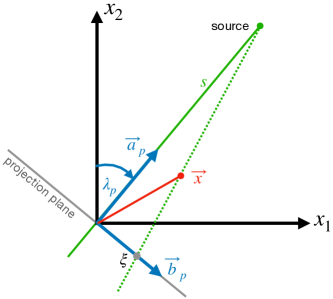
Figure 2: Scanner geometry considered in the noise reconstructions.

An illustration of the geometry is shown in figure 2. We place the rotation axis at the origin $(0,0)$. The source angle is denoted with $\lambda_{p}$ and increases clockwise, $s$ is the source to centre distance, and $\vec{a}_{\lambda_{p}}$ is the source position in two dimensional Cartesian coordinates, i.e. $\vec{a}_{\lambda_{p}}=s(\sin\lambda_{p},\cos\lambda_{p})^{T}$. The basis vector of the projection plane (1D) going through $(0,0)$ is $\vec{b}_{\lambda_{p}}=(\cos\lambda_{p},-\sin\lambda_{p})^{T}$ and $\xi$ refers to the coordinate in the projection frame. For a given point $\vec{x}=(x_{1},x_{2})^{T}$ and source angle $\lambda_{p}$, the coordinate $\xi$ in the projection frame is given by

$$\xi=\vec{x}\cdot\vec{b}_{\lambda_{p}}\frac{s}{s-\vec{x}\cdot\vec{a}_{\lambda_{p}}}=\frac{s\left(x_{1}\cos\lambda_{p}-x_{2}\sin\lambda_{p}\right)}{s-x_{1}\sin\lambda_{p}-x_{2}\cos\lambda_{p}}.$$ (9)

The position $\xi$ and angle $\lambda_{p}$ are sampled uniformly, i.e.

$$\lambda_{p} =(p-1)\Delta\lambda,\quad p=1,2,\dots,P$$ (10)

$$\xi_{j} =(j+1/2)\Delta\xi,\quad j=-J,-J+1,\dots,J-1$$ (11)

with $\Delta\lambda$ the angular spacing between projections, $P$ the number of projections, $\Delta\xi$ the pixel width in a projection, and $2J$ the number of sampled positions in the central projection plane.

We assumed that projections are filtered with an apodized ramp filter [28],

$$h_{F}(\xi_{j})=h_{F}((j+1/2)\Delta\xi)=\begin{cases}1/(2\Delta\xi)^{2}&\mathrm{for}\,j=0,\\ 0&\mathrm{for}\,j\,\text{even and}\,j\neq 0\\ -1/(j\pi\Delta\xi)^{2}&\mathrm{for}\,j\,\mathrm{odd},\end{cases}$$ (12)

and that images are reconstructed with the Feldkamp-Davis-Kress (FDK) algorithm [15], which is the case in the distance driven binning algorithm in [29]. For simplicity, we treated proton trajectories as straight lines and therefore only used one projection image per projection angle corresponding to the central depth, unlike [27] who considered the influence of multiple Coulomb scattering.

In general, the variance of the RSP value at point $\vec{x}$ is calculated by backprojecting the variance and covariance of the filtered projections, where the covariance arises from the combination of interpolation and filtering. We use a simplified version of the noise reconstruction which replaces the covariance term (for bilinear interpolation of projections filtered by the same apodized ramp filter) by an effective factor $f_{\mathrm{interp}}=2/3-2/\pi^{2}$ [27]. This avoids interference patterns in the noise distributions due to correlations among pixels and makes the results easier to interpret. In particular, the RSP variance at $\vec{x}$ is

$$\mathrm{Var}_{\mathrm{RSP}}(\vec{x})=f_{\mathrm{interp}}\frac{\Delta\lambda^{2}}{4}\sum_{p=1}^{P}\left(\frac{\|\vec{a}_{\lambda_{p}}\|}{\|\vec{x}-\vec{a}_{\lambda_{p}}\|}\right)^{4}V_{p}(\xi_{k}).$$ (13)

The term $V_{p}(\xi_{k})$ is the variance in the filtered projections at $\xi_{k}$,

$$V_{p}(\xi_{k})=(\Delta\xi)^{2}\sum_{j=-J}^{J-1}h_{F}^{2}(\xi_{k}-\xi_{j})\frac{\|\vec{a}_{\lambda_{p}}\|^{2}}{\|\vec{a}_{\lambda_{p}}\|^{2}+\xi_{j}^{2}}\mathrm{Var}(\lambda_{n},\xi_{j}),$$ (14)

where $\mathrm{Var}(\lambda_{n},\xi_{j})$ refers to the noise projection containing the WEPL variance, $\frac{\|\vec{a}_{\lambda_{p}}\|^{2}}{\|\vec{a}_{\lambda_{p}}\|^{2}+\xi_{j}^{2}}$ is a weighting factor [1].

2.3 Simulations and phantoms

We used a cylindric water phantom with a 20 cm diameter and with infinite axial extension. To simulate noise projections, we forward projected RSP values of the phantom to obtain a projection image containing WEPL values, converted these into energy loss via the inverse of equation 7, and calculated the variance projections $\mathrm{Var}(\lambda_{n},\xi_{j})$ via equation 8 as described in section 2.1. We approximated proton paths as straight lines thereby neglecting the effect of multiple Coulomb scattering. This simplified the reconstruction because distance driven binning was not necessary. Energy loss and scattering in the air was neglected, given that 1 m of air corresponds to only 1 mm of water in terms of mass density. We used 360 projection angles uniformly distributed over a full circular trajectory and assumed a source-to-center distance of 200 cm, which is representative of many modern therapeutic proton accelerators. The pixel size was $1\times 1$ mm², both in the projection images and in the reconstructed images. We considered an energy spread of the proton beam of $\delta E_{\mathrm{beam}}=0.5$% as a figure of merit [31].

We determined the number of protons contributing to a pixel in equation 8 in relation to the dose at the phantom centre of 10 mGy accumulated over an entire proton CT scan. Specifically, the fluence at the exit of the cylinder, $\Phi_{\mathrm{out}}$, i.e. the fluence of protons measurable by the energy detector, depends on the thickness of material traversed by the protons expressed in WEPL, which we denote with $W(\xi)$ and which depends on the location $\xi$ in the projection plane (but not on the source position $\lambda$ because the scanned object is a cylinder). Assuming a spatially constant initial fluence, $\Phi_{\mathrm{in}}$, one can relate $\Phi_{\mathrm{out}}(W(\xi))$ and the proton fluence at the cylinder centre $\Phi_{\mathrm{centre}}$:

$$\Phi_{\mathrm{out}}(W(\xi))=\Phi_{\mathrm{in}}\exp(-\kappa W(\xi))=\Phi_{\mathrm{centre}}\exp(-\kappa(W(\xi)-R)),$$ (15)

where $R$ is the cylinder radius and $\kappa=0.01$ cm^-1 is a coefficient describing attenuation due to nuclear interactions in water [33, 26]. $\Phi_{\mathrm{centre}}$ is related to the dose $D_{\mathrm{centre}}$ accumulated at the cylinder centre during a full pCT scan ($P$ projections) [33]:

$$\Phi_{\mathrm{centre}}=\frac{D_{\mathrm{centre}}\rho}{P\left[S(E_{\mathrm{centre}})+\kappa\gamma E_{\mathrm{centre}}\right]},$$ (16)

where $S(E_{\mathrm{centre}})$ is the proton stopping power for the proton energy at the centre, $\rho$ is the mass density of the cylinder material (in our case water, i.e. $\rho=1$ g/cm³), $\gamma$=0.65 is the fraction of energy transferred to secondary particles during nuclear interactions (in the energy range up to 200 MeV, in water-like material). In a water cylinder with $R=10$ cm radius and for a 200 MeV proton beam, one has $E_{\mathrm{centre}}\approx 151$ MeV and consequently a proton stopping power $S(E_{\mathrm{centre}})$ in water of about 5.4 MeV cm²/g [6]. With these numbers, equation 16 yields a fluence at the centre of 270 protons per mm² per projection, which corresponds well to the numbers in [33] estimated via Geant4 Monte Carlo simulation [2].

The full expression for the modelled variance projection is obtained by combining equations 8, 15, and 16,

$$\mathrm{Var}(\lambda_{p},\xi_{j})=\frac{\sigma^{2}_{E_{\mathrm{out}}}(\lambda_{p},\xi_{j})}{S_{w}^{2}(E_{\mathrm{out}}(\lambda_{p},\xi_{j}))}\frac{P\left[S(E_{\mathrm{centre}})+\kappa\gamma E_{\mathrm{centre}}\right]}{D_{\mathrm{centre}}\rho\Delta\xi^{2}}\exp(\kappa\left(W(\lambda_{p},\xi_{j})-R)\right),$$ (17)

where $W(\lambda_{p},\xi_{j})$ is the WEPL at sampling point $\xi_{j}$ in projection $\lambda_{p}$ and $E_{\mathrm{out}}(\lambda_{p},\xi_{j})$ is obtained from $W(\lambda_{p},\xi_{j})$ via the inverse of equation 7.

3 Results

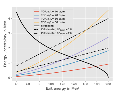
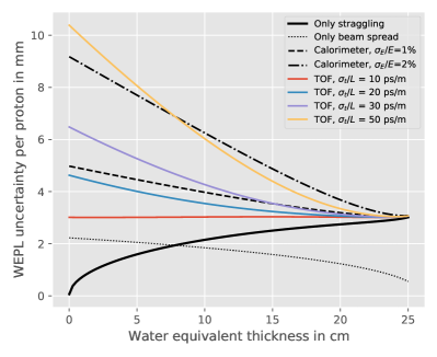
Figure 3: Left: Energy uncertainty (1 sigma) due to straggling and energy measurement error for different velocity errors $\sigma_{t}/L$ and a beam energy of 200 MeV. The dashed and dash-dotted lines depict a 1% and 2% uncertainty of a calorimeter detector, respectively. Right: WEPL uncertainty (1 sigma) of a proton CT system (equation 8) as a function of WEPL for a beam energy of 200 MeV and different velocity errors $\sigma_{t}/L$. Right: WEPL uncertainties for a calorimeter-based system (dashed, dash-dotted) are shown for comparison.

The left panel in figure 3 shows the energy uncertainty due to the energy measurement error, either via TOF (solid) or via calorimeter (dashed, dash-dotted), and due to straggling (solid black) for an incident beam energy of 200 MeV. Throughout the results section, we report all uncertainties as one sigma errors, i.e. one standard deviation. It is intuitively clear that the energy uncertainty due to TOF error decreases with decreasing exit energy because the lower the proton’s energy, the longer its time-of-flight so that the time resolution of the TOF sensors has less impact on the estimated velocity. The limit is that protons still need to reliably traverse the scanned object rather than lose all their energy inside. The lowest depicted energy value of 40 MeV corresponds to a residual range of about 1.5 cm. Straggling, on the other hand, increases with the degree to which a proton has been slowed down due to electromagnetic interactions and thus increases with decreasing exit energy.

The right panel in figure 3 shows how the combined energy uncertainty (due to straggling, measurement error, and beam spread) translates into WEPL uncertainty as a function of the phantom’s water equivalent thickness, again for a beam energy of 200 MeV. In thin objects, it is mainly the TOF error which dominates the WEPL uncertainty while it is mainly straggling in thicker objects. For velocity errors larger than 50 ps/m, the measurement error is more dominant than straggling for almost all WEPLs. Overall, the WEPL precision of a 20-30 ps/m TOF proton CT system is comparable to a calorimeter-based system with 1% energy measurement error, while a 2% calorimeter error corresponds to a velocity error $\sigma_{t}/L$ of about 50 ps/m.

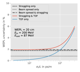
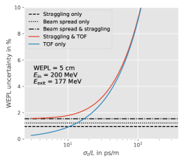
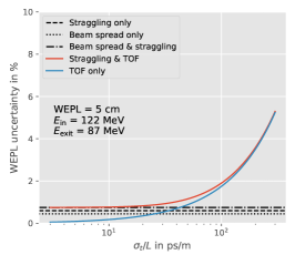
Figure 4: WEPL uncertainty in a TOF proton CT as a function of velocity error $\sigma_{t}/L$ for three different combinations of object thickness and beam energy.

Figure 4 compares the three contributions to WEPL uncertainty, i.e. straggling, TOF measurement error, and beam spread, as a function of the velocity error $\sigma_{t}/L$ for an object thickness of 5 cm and 20 cm, as indicated in the plots. With a WEPL of 20 cm, the point of equal contribution (straggling + beam spread = TOF error) is found at $\sigma_{t}/L=$100 ps/m. With a WEPL of 5 cm, on the other hand, the TOF error begins to dominate already for $\sigma_{t}/L\approx 20$ ps/m. Lowering the beam energy to 122 MeV, which corresponds to the same exit energy of 86 MeV as for the 20 cm/200 MeV case, shifts the equal contribution point to about 40 ps/m.

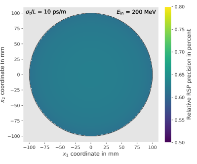
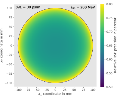
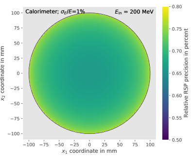
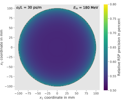
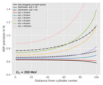
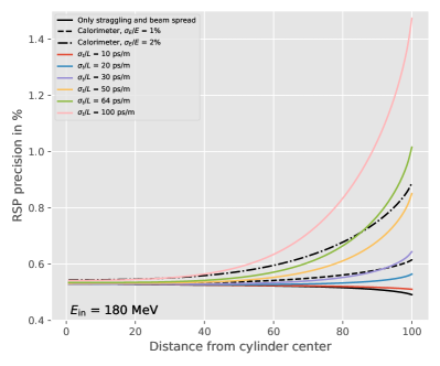
Figure 5: Upper panels: noise reconstructions of a water cylinder of 20 cm diameter for different velocity errors $\sigma_{t}/L$ and calorimeter measurement errors as well as different incident beam energies as indicated in the graphics. Lower panels: Radial profiles of the RSP precision for 200  MeV (left) and 180 MeV (right) beam energy.

The four upper panels in figure 5 show the RSP precision maps for a water cylinder with 20 cm diameter and different velocity errors $\sigma_{t}/L$ (TOF system) and $\delta E=\sigma_{E}/E$ (calorimeter system), as indicated in the graphics. The noise images were simulated as described in section 2.3 and reconstructed according to section 2.2. The two lower panels show radial noise profiles for different values of $\sigma_{t}/L$, for calorimeter precisions of $\delta E=1$% and $\delta E=2$%, and the idealised case where only straggling and the beam’s energy spread contribute to image noise. Noise is distributed quite evenly for $\sigma_{t}/L$ between 10 and 20 ps/m, while there is a marked increase towards the phantom edge for higher values of $\sigma_{t}/L$, e.g. by a factor of 1.6 for $\sigma_{t}/L$=50 ps/m. This is because WEPL uncertainty depends on WEPL (see figure 3) and in locations close to the edge, protons only traverse a thin tangential portion of the phantom under certain projection angles. The backprojection operation in the reconstruction therefore accumulates higher noise over all projections for points near the edge than for points close to the centre. A similar tendency is seen for the calorimeter-based system, where the 1% case yields noise profiles comparable to the 30 ps/m TOF system. At first sight, it seems surprising that the 50 ps/m TOF case yields better precision than the 2% calorimeter system at all distances from the centre although figure 4 suggests similar performance. This is understandable because even at a location close to the edge within the cylinder, the proton WEPL is relatively large for most projection angles and the TOF system performs better than the calorimeter-based set-up for any WEPL larger than 8 cm (figure 3). With the lower beam energy of 180 MeV, which corresponds to 1.6 cm residual range after 20 cm of water, RSP precision reaches the intrinsic limit imposed by straggling and the beam’s energy spread, at least for the inner half of the cylinder.

4 Discussion

The purpose of this work was to investigate the RSP precision in time-of-flight proton CT based on physics models and statistics. Our results show that an RSP precision of better than 1% can be achieved in a water cylinder of 20 cm and a beam energy of 200 MeV, which is representative of a human head and therapeutic proton accelerator, and with a velocity error of a few tens of ps/m. The dose to the phantom centre was 10 mGy. Note that WEPL and thus RSP variance are inversely proportional to the square root of dose (equations 8 and 16) so that lowering the dose by a factor of 10 would increase (i.e. worsen) the RSP precision by a factor of $\sqrt{10}\approx 3.14$. On the other hand, we point out that the RSP precision is inversely proportional to the fourth power of the pixel size, i.e. $\mathrm{Var}_{\mathrm{RSP}}(\vec{x})\propto\Delta\xi^{-4}$ (equation 14), where a factor of $1/\Delta\xi^{2}$ results from the filtering operation and another factor of $1/\Delta\xi^{2}$ is linked to the number of protons per pixel (equation 8) [33, 26, 19]. Thus, increasing pixel size by a factor of two from $1\times 1$ mm² to $2\times 2$ mm² would reduce (i.e. improve) RSP precision by a factor of 4.

WEPL uncertainty (and consequently RSP uncertainty) due to TOF measurement error decreases as the object thickness increases, while the opposite is true for energy straggling (figure 4). For a ratio of TOF error over distance between sensor planes of 10-20 ps/m, both effects contribute to a similar extend. For velocity errors $\sigma_{t}/L>50$ ps/m, on the other hand, it is mainly the TOF measurement dominating the RSP precision. Our results show that a 30 ps/m TOF system yields similar RSP precision with a cylindrical object of 20 cm diameter as a 1% precision calorimeter-based system (figure 5).

The dependence of WEPL uncertainty on WEPL leads to a spatially varying RSP precision in the reconstructed proton CT image. In particular, TOF proton CT images are expected to be noisier towards the object’s edges than at its centre. This effect is not specific to TOF proton CT, however, but can also be seen in calorimeter-based proton CT [27, 13], where e.g. the energy measurement error in a scintillator varies as a function of deposited energy. [4] studied this aspect and proposed a multilayer scintillator system in order to make WEPL uncertainty less dependent on WEPL. The design of a TOF proton CT system will likely require a similar kind of study to achieve homogeneous image noise. Possible ways to achieve this include energy degraders in front of the TOF system to reduce the residual energy, adapting the beam energy to the local phantom thickness [14], or modulating the beam fluence to adjust the noise distribution [12].

[39] presented a TOF proton CT prototype employing Large Area Picosecond Photon Detectors with a one sigma TOF error of 64 ps. In the setting used in this work, i.e. a water cylinder of 20 cm diameter, a dose to the centre of 10 mGy, and $1\times 1$ mm² pixels, these detectors are expected to yield similar RSP precision as a 2% calorimeter-based proton CT system (figure 5) if the TOF sensors are placed 1 m apart from each other. With a spacing of $L=10$ cm, as reported in [39], the uncertainty on the exit energy due to the TOF measurement error would increase by a factor of ten (equation 2) and the RSP precision would range from about 4% at the centre to 13% at the cylinder edge for a beam energy of 200 MeV. Keeping the spacing at 10 cm, but reducing the incident beam energy to 180 MeV, which corresponds to a range in water of 21.6 cm, the RSP at the cylinder centre would reduce to 0.9% and to 9% near the edge. [37] performed first tests in a therapeutic proton beam with a new ultra fast silicon detector based on low gain avalanche diode (LGAD) technology [22]. They report a time resolution per sensor plane of 75 ps to 115 ps, i.e. TOF errors of 106 ps to 162 ps. [30] had previously found TOF resolutions of an LGAD sensor of around 30 ps. [10] studied the performance of Chemical Vapor Deposition diamond detectors in the context of ion beam therapy monitoring and reported time resolutions on the order of 100-200 ps for protons depending on the energy, and as low as 13 ps for carbon ions. Based on our results, some of these new sensor types could be suitable for TOF proton CT in terms of time resolution. In general, it would be crucial to devise an acquisition procedure which leads to an exit energy as low as possible (figure 3 left). Furthermore, given that the RSP resolution depends on the velocity error $\sigma_{t}/L$, designing a TOF proton CT will also require engineering efforts to integrate into a treatment room a system with a large distance between the sensor planes.

Our work makes a few simplifying assumptions. First, we only consider the energy measurement error, energy straggling, and the beam’s energy spread as sources of RSP uncertainty, yet neglect noise induced by scattering in the object. [13] have studied the contribution of this source of noise in a calorimeter-based proton CT prototype [16]. The prototype is designed in such a way that energy straggling and measurement error combined lead to a WEPL uncertainty roughly independent of WEPL [4]. [13] found that noise due to scattering depends on the object shape and composition and the location of interest inside the object. The authors report that scattering noise in a homogeneous water cylinder is absent at the centre and most pronounced towards the cylinder edges where it contributes up to 20% to the RSP precision. Based on this, our RSP precision profiles (figure 5, lower panels) are expected to remain unchanged at the centre and reach about 1% for $\sigma_{t}/L=$ 30 ps/m if noise due to scattering is considered.

Another simplification is that our reconstruction uses straight proton lines instead of curved most likely paths. This implies that our noise images (figure 5) are slightly blurrier than how they would be if we had implemented a reconstruction algorithm which considers the MLP, such as distance driven binning [29, 27]. Given that RSP precision increases smoothly towards the edge, this simplification has no relevant impact on the results reported here. Note that using straight lines in the noise reconstruction and neglecting the contribution of MCS to image noise are two distinct aspects. The former causes the noise maps to be blurred while the latter may cause an underestimation of the noise level (see previous paragraph).

As the purpose of this work was to characterise a proton CT modality, we have only considered direct reconstruction algorithms, and in particular the distance driven method described in [29]. Other direct methods exist, but have been shown to yield very similar results in terms of image noise and spatial resolution [18]. We have not considered iterative reconstruction methods because image properties strongly depend on the parameters of the reconstruction, such as regularisation weights [24, 25].

5 Conclusion

The purpose of this work was to investigate the RSP precision in proton CT if TOF is used as energy measurement mechanism. The three noise contributions we considered were the TOF measurement error in relation to the spacing between the TOF sensor planes, the energy straggling experienced by the protons inside the scanned objects, as well as the proton beam’s energy spread. For comparison, we also considered a calorimeter-based set-up which has been implemented in prototype scanners. Which of the three contributions dominates depends on the combination of beam energy and object thickness. For objects of up to 20 cm and a beam energy of 200 MeV, we find that beam spread and straggling are similarly relevant as the measurement error for velocity errors in the range of 10-50 ps/m. In TOF proton CT systems with a distance between the sensor planes of one metre and a time resolution of 100 ps or larger, the measurement error tends to be the most dominant source of RSP uncertainty unless the beam energy is chosen such that the exit energy is very low (<80 MeV). TOF proton CT images of a 20 cm diameter water cylinder acquired at 10 mGy total dose to the object centre and reconstructed with a pixel size of 1 mm² have an RSP precision of 1% or better when the velocity error is 50 ps/m or lower. RSP precision varies spatially in a TOF proton CT image and generally increases towards the object’s edges. This is similar to, but more pronounced than, previously reported results for calorimeter-based proton CT systems. A calorimeter-based system with 1% energy error is comparable to a TOF-based system with a velocity error of 30 ps/m, and a 2% calorimeter system corresponds to a 64 ps/m TOF system. Overall, we expect that better precision and more homogeneous image noise can be achieved by optimally adapting the beam energy to the phantom’s water equivalent thickness.

References

References

- [1] A. Kak et al. “3. Algorithms for Reconstruction with Nondiffracting Sources” In Principles of Computerized Tomographic Imaging Society for IndustrialApplied Mathematics, 2001, pp. 49–112 DOI: 10.1137/1.9780898719277.ch3
- [2] S. Agostinelli et al. “GEANT4 - A simulation toolkit” In Nuclear Instruments and Methods in Physics Research, Section A: Accelerators, Spectrometers, Detectors and Associated Equipment 506.3, 2003, pp. 250–303 DOI: 10.1016/S0168-9002(03)01368-8
- [3] Johan Alme et al. “A High-Granularity Digital Tracking Calorimeter Optimized for Proton CT” In Frontiers in Physics 8, 2020 DOI: 10.3389/fphy.2020.568243
- [4] V. A. Bashkirov et al. “Novel scintillation detector design and performance for proton radiography and computed tomography” In Medical Physics 43.2, 2016, pp. 664–674 DOI: 10.1118/1.4939255
- [5] M. J. Berger et al. “Report 49” In Journal of the International Commission on Radiation Units and Measurements os25.2, 1993 DOI: 10.1093/jicru/os25.2.Report49
- [6] M.J. Berger et al. “ESTAR, PSTAR, and ASTAR: Computer Programs for Calculating Stopping-Power and Range Tables for Electrons, Protons, and Helium Ions (version 1.2.3)” In National Institute of Standards and Technology, 2005 DOI: 10.18434/T4NC7P
- [7] C Bopp et al. “Quantitative proton imaging from multiple physics processes: a proof of concept.” In Physics in medicine and biology 60.13, 2015, pp. 5325–41 DOI: 10.1088/0031-9155/60/13/5325
- [8] C. Civinini et al. “Recent results on the development of a proton computed tomography system” In Nuclear Instruments and Methods in Physics Research, Section A: Accelerators, Spectrometers, Detectors and Associated Equipment 732 Elsevier, 2013, pp. 573–576 DOI: 10.1016/j.nima.2013.05.147
- [9] Charles-Antoine Collins-Fekete et al. “Statistical limitations in ion imaging” In Physics in Medicine & Biology 66.10, 2021, pp. 105009 DOI: 10.1088/1361-6560/abee57
- [10] Sébastien Curtoni et al. “Performance of CVD diamond detectors for single ion beam-tagging applications in hadrontherapy monitoring” In Nuclear Instruments and Methods in Physics Research Section A: Accelerators, Spectrometers, Detectors and Associated Equipment 1015, 2021, pp. 165757 DOI: 10.1016/j.nima.2021.165757
- [11] Ethan A. DeJongh et al. “Technical Note: A fast and monolithic prototype clinical proton radiography system optimized for pencil beam scanning” In Medical Physics 48.3, 2021, pp. 1356–1364 DOI: 10.1002/mp.14700
- [12] J. Dickmann et al. “An optimization algorithm for dose reduction with fluence–modulated proton CT” In Medical Physics, 2020, pp. mp.14084 DOI: 10.1002/mp.14084
- [13] Jannis Dickmann et al. “Prediction of image noise contributions in proton computed tomography and comparison to measurements” In Physics in Medicine & Biology 64.14, 2019, pp. 145016 DOI: 10.1088/1361-6560/ab2474
- [14] Jannis Dickmann et al. “Proof of concept image artifact reduction by energy-modulated proton computed tomography (EMpCT)” In Physica Medica 81, 2021, pp. 237–244 DOI: 10.1016/j.ejmp.2020.12.012
- [15] L. a. Feldkamp et al. “Practical cone-beam algorithm” In Journal of the Optical Society of America A 1.6, 1984, pp. 612 DOI: 10.1364/JOSAA.1.000612
- [16] R P Johnson et al. “A Fast Experimental Scanner for Proton CT: Technical Performance and First Experience With Phantom Scans” In IEEE Transactions on Nuclear Science 63.1, 2016, pp. 52–60 DOI: 10.1109/TNS.2015.2491918
- [17] Robert P Johnson “Review of medical radiography and tomography with proton beams” In Reports on Progress in Physics 81.1, 2018, pp. 016701 DOI: 10.1088/1361-6633/aa8b1d
- [18] Feriel Khellaf et al. “A comparison of direct reconstruction algorithms in proton computed tomography” In Physics in Medicine & Biology 65.10, 2020, pp. 105010 DOI: 10.1088/1361-6560/ab7d53
- [19] Nils Krah et al. “Scattering proton CT” In Physics in Medicine & Biology 65.22, 2020, pp. 225015 DOI: 10.1088/1361-6560/abbd18
- [20] Harald Paganetti “Proton Therapy Physics” Boca Raton: Taylor & Francis Group, 2012
- [21] M. G. Payne “Energy Straggling of Heavy Charged Particles in Thick Absorbers” In Physical Review 185.2, 1969, pp. 611–623 DOI: 10.1103/PhysRev.185.611
- [22] G. Pellegrini et al. “Technology developments and first measurements of Low Gain Avalanche Detectors (LGAD) for high energy physics applications” In Nuclear Instruments and Methods in Physics Research Section A: Accelerators, Spectrometers, Detectors and Associated Equipment 765, 2014, pp. 12–16 DOI: 10.1016/j.nima.2014.06.008
- [23] P Pemler et al. “A detector system for proton radiography on the gantry of the Paul-Scherrer-Institute” In Nuclear Instruments and Methods in Physics Research Section A: Accelerators, Spectrometers, Detectors and Associated Equipment 432.2-3, 1999, pp. 483–495 DOI: DOI: 10.1016/S0168-9002(99)00284-3
- [24] S N Penfold et al. “Total variation superiorization schemes in proton computed tomography image reconstruction.” In Medical physics 37.11, 2010, pp. 5887–5895 DOI: 10.1118/1.3504603
- [25] Scott Penfold et al. “Techniques in Iterative Proton CT Image Reconstruction” In Sensing and Imaging 16.1, 2015, pp. 19 DOI: 10.1007/s11220-015-0122-3
- [26] C T Quiñones et al. “Filtered back-projection reconstruction for attenuation proton CT along most likely paths” In Physics in Medicine and Biology 61.9, 2016, pp. 3258–3278 DOI: 10.1088/0031-9155/61/9/3258
- [27] Martin Rädler et al. “Two-dimensional noise reconstruction in proton computed tomography using distance-driven filtered back-projection of simulated projections” In Physics in Medicine & Biology 63.21, 2018, pp. 215009 DOI: 10.1088/1361-6560/aae5c9
- [28] G. N. Ramachandran et al. “Three-dimensional Reconstruction from Radiographs and Electron Micrographs: Application of Convolutions instead of Fourier Transforms” In Proceedings of the National Academy of Sciences 68.9, 1971, pp. 2236–2240 DOI: 10.1073/pnas.68.9.2236
- [29] Simon Rit et al. “Filtered backprojection proton CT reconstruction along most likely paths.” In Medical physics 40.3, 2013, pp. 031103 DOI: 10.1118/1.4789589
- [30] Hartmut F-W Sadrozinski et al. “4D tracking with ultra-fast silicon detectors” In Reports on Progress in Physics 81.2, 2018, pp. 026101 DOI: 10.1088/1361-6633/aa94d3
- [31] Jacobus Maarten Schippers “Beam Transport Systems for Particle Therapy” In Proceedings of the CAS-CERN Accelerator School: Accelerators for Medical Applications, Vösendorf, Austria: CERN, 2018 DOI: 10.23730/CYRSP-2017-001.241
- [32] R. W. Schulte et al. “A maximum likelihood proton path formalism for application in proton computed tomography” In Medical Physics 35.11 American Association of Physicists in Medicine, 2008, pp. 4849 DOI: 10.1118/1.2986139
- [33] Reinhard W. Schulte et al. “Density resolution of proton computed tomography” In Medical Physics 32.4 AAPM, 2005, pp. 1035–1046 DOI: 10.1118/1.1884906
- [34] J. T. Taylor et al. “An experimental demonstration of a new type of proton computed tomography using a novel silicon tracking detector” In Medical Physics 43.11, 2016, pp. 6129–6136 DOI: 10.1118/1.4965809
- [35] C. Tschalär “Straggling distributions of large energy losses” In Nuclear Instruments and Methods 61.2, 1968, pp. 141–156 DOI: 10.1016/0029-554X(68)90535-1
- [36] Felix Ulrich-Pur et al. “Feasibility study of a proton CT system based on 4D-tracking and residual energy determination via time-of-flight”, 2021 URL: http://arxiv.org/abs/2109.05058
- [37] A Vignati et al. “A new detector for the beam energy measurement in proton therapy: a feasibility study” In Physics in Medicine & Biology 65.21, 2020, pp. 215030 DOI: 10.1088/1361-6560/abab58
- [38] Lennart Volz “Particle imaging for daily in-room image guidance in particle therapy”, 2020, pp. 281 DOI: 10.11588/heidok.00029273
- [39] William A. Worstell et al. “First results developing time-of-flight proton radiography for proton therapy applications” In Medical Imaging 2019: Physics of Medical Imaging SPIE, 2019, pp. 15 DOI: 10.1117/12.2511804
- [40] Adam Wunderlich et al. “Image covariance and lesion detectability in direct fan-beam x-ray computed tomography” In Physics in Medicine and Biology 53.10, 2008, pp. 2471–2493 DOI: 10.1088/0031-9155/53/10/002