Study of voltage cycling conditions on Pt oxidation and dissolution in polymer electrolyte fuel cells

Abstract

This paper is devoted to study the electrochemical behavior of Pt catalyst in a polymer electrolyte fuel cell at various operating conditions and at different electric potential difference (also known as voltage) cycling applied in accelerated stress tests. The degradation of platinum is considered with respect to the Pt ion dissolution and the Pt oxide coverage of catalyst described by a one-dimensional model. In the model, degradation rate increases with temperature and decreasing particle diameter of Pt nano-particles. The theoretical study of the underlying diffusion system with the nonlinear reactions is presented by analytical methods and gives explicit solutions through a first integral of the ODE system. Numerical tests are obtained using a second order implicit-explicit scheme. The computer simulation shows that the lifetime of the catalyst depends on the voltage profile and the upper potential level. By this Pt mass loss is more significant at the membrane surface than at the gas diffusion layer.

1 Introduction

At present, the polymer electrolyte fuel cells are very extensively developed as power sources for application in portable computers, heating systems as well for leisure yachts, aircraft and vehicles [1, 2, 3, 4]. In commercial PEM fuel cells, the most used material for catalyst is platinum. Effective usage of this valuable metal is challenging task in elaboration of the modern fuel cell systems with high durability and long lifetime.

Mathematical modelling helps to better understand phenomena causing the chemical degradation on the Pt surface and allows predicting a decline in electro-chemical surface area (ECSA) of the catalyst and effectivity of the fuel cell [5, 6, 7]. In the last decades, numerous publications have been devoted to develop mathematical models prediction Pt oxidation and dissolution in the catalyst layer of PEMFCs. In 2007, Zhang et al [8] suggested a simple model accounting Pt dissolution and further precipitation within the membrane of PEMFCs. One year late, Bi and Fuller [9] published a dynamic model applied to estimate Pt mass loss during potential cycling. In 2009, Holby et al. [10] developed a kinetic model taking into account effect of Pt particle size on the rate of the degradation. It was demonstated that, due to rapid changes in the Gibbs–Thomson energy, particle size effects dominate degradation for 2 nm particles but play almost no role for 5 nm particles. In 2015 Hiraoka et al. [11] proposed a model for the Pt particle growth based on the Gibbs–Thomson equation and simulated change in the Pt particle size distribution during electric potential cycling. Using the developed model, the authors investigated an effect of high potential limit and Pt particle diameter on particle size growth. The results showed that lowing high potential in the cycling the Pt particle size grows more slowly. A decrease in particle size accelerates Pt dissolution. In the same year, Li et al. [12] published a mathematical model taking into account effect of RH, T and catalyst layer thickness on the loss in electrochemical active area of the Pt catalyst. The simulation results were in good agreement with experiments. The conducted simulation for a triangle potential cycle demonstrated that thinning the cathode catalyst layer would induce more rapid ECSA loss. ECSA increases with rising temperature and higher relative humidity. In 2018, using a simplified model Baricci et al. [13] studied changes in roughness through the catalyst layer thickness. Non-uniform degradation is observed in the catalyst layer consequently to the formation of a platinum depleted region next to the membrane, which, according to the model, results from diffusion and precipitation of dissolved platinum into the membrane. Recently, Koltsiva et al. [14] suggested a novel model, which for the first time considers five phenomena simultaneously proceeding on the Pt/C catalyst surface: platinum nanoparticles electrochemical dissolution, particle growth due to Ostwald ripening, migration of nanoparticles along the carbon support, coalescence of fine particles, diffusion of platinum ions in the ionomer.

The present paper is focused on study the effect of kind of voltage cycling, where voltage is commonly adopted as electric potential difference versus a reference of 0 (V), on the electro-chemical behavior of Pt catalyst in a polymer electrolyte fuel cell (PEFC). For this purpose we have developed a mathematical model based on the physico-chemical data of the Pt dissolution and oxidation reactions and taking account diffusion of building Pt ions into the ionomer membrane. The two degradation phenomena of the platinum ion (Pt²⁺) dissolution and the platinum oxide (PtO) formation of Pt catalyst layer (coverage) in polymer-electrolyte membrane fuel cells (PEMFC) are studied theoretically at different voltage cycling conditions. To describe these phenomena, the degradation model due to Holby [15, 10] is utilized, which is one-dimensional (1d) across the catalyst layer (CL) thickness and accounts for diffusion of Pt ions. For mathematical modeling of interface reactions in multi-phase media within complete electrokinetic Poisson–Nernst–Planck equations, see e.g. [16, 17, 18]. For mathematical approaches which are suitable to describe and to test a mechanical degradation due to fracture phenomena, we refer to [19, 20, 21].

The paper is organized in the following way: after the introduction we describe theoretical approach developed, where the part “Degradation model of Pt catalyst” displays geometrical, physical and chemical properties of the catalyst layer and the ionomer membrane used for further simulation; “Theoretical and numerical methods” introduces the mathematical and the numerical models; “Results” presents simulation results and their discussion; “Discussion” and “Conclusion” summarize the most important findings of the current study. The mathematical model is given by a coupled system of nonlinear reaction-diffusion equations with modified Butler–Volmer reaction rates for three unknown variables: Pt²⁺ concentration, Pt particle diameter, and PtO coverage ratio. For its numerical solution we use a second order implicit-explicit scheme following [22]. Neglecting diffusion of Pt ions, in A the resulting nonlinear reaction equations are reduced to two unknown variables with the help of a first integral of the system, while in B an example of analytical solution is constructed.

2 Degradation model of Pt catalyst

Approximations

The developed model of the Platinum on carbon (Pt/C) degradation is based on the following approximations:

• This is a one-dimensional and a dynamic model.

• The model considers two layers of a polymer electrolyte fuel cell (PEFC): the cathode catalyst layer (CL) with length $L_{\rm CL}$ and the polymer electrolyte membrane (PEM) with length $L_{\rm PEM}$. The catalyst layer is filled with catalyst particles: spherical Pt nano-particles placed on C-support bound with the membrane by perfluorinated sulfonated ionomer, the membrane is made from the same ionomer.

• The degradation of Pt nano-particles are caused by Pt oxidation and Pt dissolution, which are described by the following electro-chemical reactions:

  $${\rm Pt}_{\rm(s)}\longleftrightarrow{\rm Pt}^{2+}_{\rm(aq)}+2{\rm e}^{-},$$ (1a)

  $${\rm Pt}_{\rm(s)}+{\rm H}_{2}{\rm O}_{\rm(aq)}\longleftrightarrow{\rm PtO}_{\rm(s)}+2{\rm H}^{+}_{\rm(aq)}+2{\rm e}^{-}.$$ (1b)

• The rates of the degradation reactions (1) are simulated by a modified Butler–Volmer equation (see (3) and (4)) taking into account Gibbs–Thomson’s effect: dependence of a surface potential on nano-particle size as well as influence of the surface potential on the potential gradient in the system.

• The platinum ions occurring due to the Pt dissolution (1) diffuse through the ionomer phase of the catalyst layer into the polymer electrolyte membrane. The diffusion of Pt ions into the gas diffusion layer is impossible because this layer does not possess ionic conductivity. This determines boundary conditions (5e) for the Pt ions diffusion (5a).

• On balance, the model takes into account an effect of potential gradient, Pt particle size, temperature, relative humidity as well as other phenomena (see parameter gathered in Table 1) on the degradation rates of platinum catalyst and allows calculating the platinum ion concentration (${\rm Pt}^{2+}$), the particle diameter, and the platinum oxide (PtO) coverage ratio from governing relations (5).

With respect to the relative humidity in point 6 we remark the following. In our model we consider an effect of pH on the reaction rate of Pt oxidation. The pH depends on the dissociation degree of sulfonyl groups of the ionomer. In the simulated cases we suppose that the sulfonyl groups are completely dissociated and $pH=0$. Generally, pH is function of proton concentration, in PEMFCs pH depends on relative humidity.

Model variables

For a semi-infinite cathode catalyst layer of thickness $L$, we introduce a spatial variable $x\in[0,L]$ across the CL such that one end point $x=0$ corresponds to the CL-gas diffusion layer (GDL) interface, and the other end point $x=L$ confirms the CL-PEM interface. By this, we allow non-steady state operating conditions for CL with respect to time $t\geq 0$ and the spatial dependence on $x\in[0,L]$ due to diffusion phenomena. The model of degradation is sketched in Figure 1.

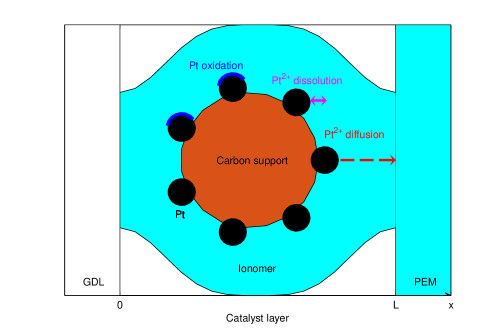
Figure 1: The model of degradation.

We emphasize that Figure 1 shows a schematic of the model configuration, when the Pt particles are fully surrounded by ionomer on the carbon support. The real scenario at Pt particles has a partial coverage by ionomer (for ion transfer) and a partial coverage by carbon network (for electron transfer) and a partial open space to air or gas (for oxygen gas diffusion). However, those factors are not addressed in the current model.

Let Pt particles be hemispheres posed with density $\rho_{\rm Pt}$ and loading $p_{\rm Pt}$ on a carbon support, such that the Pt volume fraction across CL can be estimated as follows $\varepsilon_{\rm Pt}=\frac{p_{\rm Pt}/\rho_{\rm Pt}}{L}$ with $\varepsilon_{\rm Pt}<1$. The Pt nanoparticle is assumed to be spherical of diameter $d_{\rm Pt}$ and volume $V_{\rm Pt}=\frac{4}{3}\pi(\frac{d_{\rm Pt}}{2})^{3}$. Then the Pt number concentration in CL is $N_{\rm Pt}=\frac{\varepsilon_{\rm Pt}}{V_{\rm Pt}}$. For the parameter values from Table 1, $\varepsilon_{\rm Pt}\approx 2$%, $V_{\rm Pt}\approx 1.5\times 10^{-20}$ $({\rm cm}^{3})$, and $N_{\rm Pt}\approx 1.32\times 10^{18}$ $(1/{\rm cm}^{3})$.

The unknown constituents entering (1) are the ${\rm Pt}^{2+}$ concentration $c$ (mol/cm³), Pt particle diameter $d$ (cm), and PtO coverage ratio $\theta$, that are the time-space dependent functions such that

$$c(t,x)\geq 0,\quad d(t,x)\geq 0,\quad 0\leq\theta(t,x)\leq 1.$$ (2)

Based on a modified Butler–Volmer equation, the following reaction rates in units of mol/(cm${}^{2}\cdot$s) are established in [15]: for the Pt ion dissolution (1a):

$$r_{\rm dissol}(c,d,\theta,V)=B_{1}(d,\theta)e^{(1-\beta_{1})B_{4}(d,\theta)V}-cB_{2}(d,\theta)e^{-\beta_{1}B_{4}(d,\theta)V},$$ (3a)

where the quantities $$B_{1} {}^{2}\cdot B_{2} B_{4} \gamma_{0}$$ in mol/(cms), in cm/s, in C/J, and in J/cm² are

$$\begin{split}&B_{1}(d,\theta)=\nu_{1}\mathit{\Gamma}(1-\theta)e^{\frac{1}{RT}(-H_{1,{\rm fit}}-nF(1-\beta_{1})(U_{\rm eq}-\frac{4\mathit{\Omega}\gamma_{0}(\theta)}{nFd}))},\\ &B_{2}(d,\theta)={\textstyle\frac{\nu_{2}\mathit{\Gamma}}{c_{\rm ref}}}(1-\theta)e^{\frac{1}{RT}(-H_{1,{\rm fit}}+nF\beta_{1}(U_{\rm eq}-\frac{4\mathit{\Omega}\gamma_{0}(\theta)}{nFd}))},\\ &B_{4}(d,\theta)={\textstyle\frac{F}{RT}}(n-{\textstyle\frac{4\mathit{\Omega}\mathit{\Gamma}n_{2}\theta}{d}}),\\ &\gamma_{0}(\theta)=\gamma+\mathit{\Gamma}RT\bigl{(}\theta\ln({\textstyle\frac{\nu_{2}^{\star}}{\nu_{1}^{\star}}}10^{-2pH})+\theta{\textstyle\frac{2n_{2}FU_{\rm fit}+\omega\theta}{2RT}}+\theta\ln({\textstyle\frac{\theta}{2}})+(2-\theta)\ln(1-{\textstyle\frac{\theta}{2}})\bigr{)};\end{split}$$ (3b)

for the Pt oxide coverage (1b):

$$r_{\rm oxide}(\theta,V)=\mathit{\Gamma}e^{-\frac{1}{RT}(H_{2,{\rm fit}}+\lambda\theta)}\bigl{(}\nu_{1}^{\star}(1-{\textstyle\frac{\theta}{2}})e^{-\frac{n_{2}F(1-\beta_{2})}{RT}(U_{\rm fit}+\frac{\omega\theta}{n_{2}F})+(1-\beta_{2})\frac{n_{2}F}{RT}V}\\ -\nu_{2}^{\star}10^{-2pH}e^{\frac{n_{2}F\beta_{2}}{RT}(U_{\rm fit}+\frac{\omega\theta}{n_{2}F})-\beta_{2}\frac{n_{2}F}{RT}V}\bigr{)}.$$ (4)

The terms in (3) and (4) are rearranged in such a way to express explicitly the dependence of the governing relations on the voltage $V$.

For the parameters from Table 1, the reactions rates are illustrated in Figure 2 with respect to varying $V\in[0.9,1.2]$ (V).

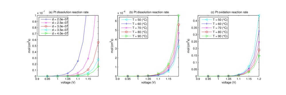
Figure 2: The reaction rates $r_{\rm dissol}$ (a), (b), and $r_{\rm oxide}$ (c) for fixed $c$ and $\theta$.

This range corresponds to the operating conditions. In Figure 2, there are fixed $c=3\times 10^{-10}$ (mol/cm³) and $\theta=0$, the five curves $V\mapsto r_{\rm dissol}(c,d,\theta,\,\cdot\,)$ in plot (a) correspond to five Pt particle diameters selected equidistantly in the range of $d\in[2,4]\times 10^{-7}$ (cm), while $r_{\rm oxide}$ is independent of $d$. For fixed $d=3\times 10^{-7}$ (cm), the curves $V\mapsto r_{\rm dissol}(c,d,\theta,\,\cdot\,)$ in (b) and $V\mapsto r_{\rm oxide}(c,\,\cdot\,)$ in (c) are plotted when varying the temperature $T\in[323.15,363.15]$ (K). Figure 2 demonstrates rates of the forward reactions: platinum dissolution (a, b) and formation of platinum oxide (c) as function of applied potential gradient at different diameters of Pt particle (a) and at different temperature (b, c). As seen from the figures the rate of platinum dissolution increases with decrease of the diameter of the platinum particles. The rate of the both reactions grow with increasing temperature.

Here it is worth noting that the rates of dissolution and re-deposition reactions are not the same. Figure 2 shows the rates only forward reactions. The model considers dissolution and re-deposition reactions, as well as building of platinum oxide (forward reaction, platinum oxidation) and reduction of platinum oxide to platinum (backward reaction).

Since the dependence of $r_{\rm dissol}$ on the Pt concentration $c$ in (3a) is linear, for large values of $c$ the backward dissolution reaction rate (having the negative sign) dominates over forward reactions (having the positive sign). In these examples, we depict the forward dissolution reaction rates when varying $V$. In Figure 2 (a) we observe decay of the dissolution reaction rates when the particle diameter $d$ increases. From Figure 2 (b) and (c) we conclude that increasing the temperature $T$ follows growth of the dissolution reaction rate and decay of the oxidation reaction rate.

3 Theoretical and numerical methods

Governing relations

For a given voltage $V$ in (3) and (4), in [12] the following system of reaction-diffusion equations is formulated: find a triple $(c,d,\theta)$ satisfying (2) such that

$${\textstyle\frac{\partial c}{\partial t}}-\sqrt{\varepsilon}D_{\rm Pt}{\textstyle\frac{\partial^{2}c}{\partial x^{2}}}=B_{3}d^{2}r_{\rm dissol}(c,d,\theta)\quad\text{for $t>0$, $x\in(0,L)$},$$ (5a)

where $$B_{3}={\textstyle\frac{\pi N_{\rm Pt}}{2\varepsilon}}$$ (1/cm³) is denoted for short,

$${\textstyle\frac{\partial d}{\partial t}}=-\mathit{\Omega}\,r_{\rm dissol}(c,d,\theta)\quad\text{for $t>0$, $x\in(0,L)$},$$ (5b)

$${\textstyle\frac{\partial\theta}{\partial t}}+{\textstyle\frac{2\theta}{d}}{\textstyle\frac{\partial d}{\partial t}}={\textstyle\frac{r_{\rm oxide}(\theta)}{\mathit{\Gamma}}}\quad\text{for $t>0$, $x\in(0,L)$};$$ (5c)

which is endowed with the initial conditions:

$$c=0,\quad d=d_{\rm Pt},\quad\theta=0\quad\text{as $t=0$, $x\in[0,L]$};$$ (5d)

and the mixed Neumann–Dirichlet boundary conditions:

$${\textstyle\frac{\partial c}{\partial x}}=0\quad\text{as $t>0$, $x=0$};\quad c=0\quad\text{as $t>0$, $x=L$}.$$ (5e)

The first equality in (5e) implies no-flux condition at the CL-GDL interface, the second condition at the CL-membrane interface assumes that the dissolved ${\rm Pt}^{2+}$ concentration goes to zero.

Neglecting the dependence on the space variable $x$, thus omitting the diffusion term (the second one) in the left-hand side of (5a) and the boundary conditions (5e), the resulting ordinary differential equations (ODE) system is studied theoretically in A. In fact, the problem is reduced to the two unknowns by finding a first integral of the system. In B a particular solution is constructed analytically under specific assumptions. The exact solution is used to test numerical solvers for the problem. Next we will investigate the initial boundary value problem (5) numerically.

Numerical algorithm

In order to solve the nonlinear reaction-diffusion equation (5a), below we develop a second order implicit-explicit (IMEX2) scheme following [22].

Let the half-strip $[0,\infty)\times[0,L]$ be meshed with temporal points $(t^{0},\dots,t^{M},\dots)$, where $t_{0}=0$, and with $N+1$ spacial points $(x_{0},\dots,x_{N})$, where $x_{0}=0$ and $x_{N}=L$. For $l=1,\dots,M$, we look for a triple of discrete functions

$$c^{l}_{h}=(c^{l}_{0},\dots,c^{l}_{N}),\quad d^{l}_{h}=(d^{l}_{0},\dots,d^{l}_{N}),\quad\theta^{l}_{h}=(\theta^{l}_{0},\dots,\theta^{l}_{N}),$$

with given $c^{0}_{h}=\theta^{0}_{h}=0$ and $d^{0}_{h}=d_{\rm Pt}$ according to the initial condition (5d). On the space mesh, forward $D^{+}c^{l}_{i}={\textstyle\frac{c^{l}_{i+1}-c^{l}_{i}}{x_{i+1}-x_{i}}}$ and backward $D^{-}c^{l}_{i}={\textstyle\frac{c^{l}_{i}-c^{l}_{i-1}}{x_{i}-x_{i-1}}}$ differences for $i=1,\dots,N-1$ are used for the standard approximation of the second-order derivative

$$[D^{-}D^{+}]c^{l}_{i}={\textstyle\frac{1}{x_{i}-x_{i-1}}}\bigl{(}{\textstyle\frac{c^{l}_{i+1}-c^{l}_{i}}{x_{i+1}-x_{i}}}-{\textstyle\frac{c^{l}_{i}-c^{l}_{i-1}}{x_{i}-x_{i-1}}}\bigr{)}.$$

We discretize (5) and iterate for $l=1,\dots,M$ with the time size $\tau^{l}=t^{l}-t^{l-1}$ two implicit-explicit equations as follows

$$\begin{cases}c^{l-1/2}_{h}-w\tau^{l}\sqrt{\varepsilon}D_{\rm Pt}[D^{-}D^{+}]c^{l-1/2}_{h}=c^{l-1}_{h}+w\tau^{l}B_{3}(d^{l}_{h})^{2}r_{\rm dissol}(c^{l-1}_{h},d^{l}_{h},\theta^{l}_{h})\\[8.61108pt] c^{l}_{h}=c^{l-1}_{h}+\tau^{l}\bigl{(}\sqrt{\varepsilon}D_{\rm Pt}[D^{-}D^{+}]c^{l-1/2}_{h}+B_{3}(d^{l}_{h})^{2}r_{\rm dissol}(c^{l-1/2}_{h},d^{l}_{h},\theta^{l}_{h})\bigr{)},\end{cases}$$ (6a)

where the IMEX parameter $$w=0.5$$ is set in the first equation, and

$$d^{l}_{h}=d^{l-1}_{h}-\tau^{l}\mathit{\Omega}\,r_{\rm dissol}(c^{l-1}_{h},d^{l-1}_{h},\theta^{l-1}_{h}),$$ (6b)

$$\theta^{l}_{h}=\theta^{l-1}_{h}+\tau^{l}\bigl{(}{\textstyle\frac{r_{\rm oxide}(\theta^{l-1}_{h})}{\mathit{\Gamma}}}+{\textstyle\frac{2\mathit{\Omega}\theta^{l-1}_{h}}{d^{l-1}_{h}}}\,r_{\rm dissol}(c^{l-1}_{h},d^{l-1}_{h},\theta^{l-1}_{h})\bigr{)}.$$ (6c)

The diffusion-reaction equations in (6a) are endowed by the boundary conditions according to (5e):

$$c^{l-1/2}_{1}=c^{l-1/2}_{0},\quad c^{l}_{1}=c^{l}_{0},\quad c^{l-1/2}_{N}=c^{l}_{N}=0.$$ (6d)

The standard TDMA algorithm is applied for inversion of a tridiagonal matrix in the implicit equation (the first one) in (6a). For solution of the nonlinear reaction equations (6b) and (6c), we apply the standard fourth order Runge–Kutta (RK4) method.

In the numerical examples reported further we set the uniform mesh of the time step size $\tau=[10^{-4},10^{-2}]$ (s), and the space step size $h=\frac{L}{10}$ (cm) when $N=10$. We note that impulse switching of voltage (see Figure 3 plot (b)) requires the smaller time step $\tau=10^{-4}$ for stable calculation, thus increasing the computational complexity. The time step $\tau$ was fixed during the iteration. The $(\tau,h)$-step choice is conform to the fact, that for large time steps the CFL-condition may be violated, thus leading to numerical instabilities. The instability appears in such manner that the oxide coverage as well as the particle diameter and the Pt2+ concentration becoming negative.

4 Results

Simulation setup

We start with parameter values given in Table 1 at the temperature $T=353.15$ (K) and constant voltage $V=0.65$ (V) that will be used for numerical simulation.

Symbol	Value	Units	Description	Ref.
Catalyst layer parameters
$L$	$1\times 10^{-3}$	cm	Thickness of cathode CL
$d_{\rm Pt}$	$3\times 10^{-7}$	cm	diameter of Pt nanoparticle
$p_{\rm Pt}$	$4\times 10^{-4}$	g/cm2	Pt loading
$\rho_{\rm Pt}$	21.45	g/cm3	density of Pt nanoparticle
$\varepsilon$	0.2		Volume fraction of ionomer increment in cathode	[12]
Physical constants
$R$	8.31445985	J/mol/K	Gas constant	[23]
$F$	96485.3329	C/mol	Faraday constant	[23]
Parameters for $Pt^{2+}$ formation and diffusion
$\nu_{1}$	$1\times 10^{4}$	Hz	Dissolution attempt frequency	[12]
$\nu_{2}$	$8\times 10^{5}$	Hz	Backward dissolution rate factor	[12]
$\beta_{1}$	0.5		Butler–Volmer transfer coefficient for Pt dissolution	[12]
$n$	2		Electrons transferred during Pt dissolution
$U_{\rm eq}$	1.18	V	Pt dissolution bulk equilibrium voltage	[24]
$\mathit{\Omega}$	9.09	cm3/mol	Molar volume of Pt	[12]
$\gamma$	$2.4\times 10^{-4}$	J/cm2	Pt [1 1 1] surface tension	[12]
$c_{\rm ref}$	$1$	mol/cm3	reference $Pt^{2+}$ concentration	[15]
$H_{1,{\rm fit}}$	$4\times 10^{4}$	J/mol	Fit Pt dissolution activation enthalpy	[12]
$D_{\rm Pt}$	$1\times 10^{-6}$	cm2/s	Diffusion coefficient of Pt2+ in the membrane	[25]
Parameters for Pt oxide formation
$pH$	0		Potential of hydrogen ions (protons)
$\nu_{1}^{\star}$	$1\times 10^{4}$	Hz	Forward Pt oxide formation rate constant	[12]
$\nu_{2}^{\star}$	$2\times 10^{-2}$	Hz	Backward Pt oxide formation rate constant	[12]
$\mathit{\Gamma}$	$2.2\times 10^{-9}$	mol/cm2	Pt surface site density	[12]
$\beta_{2}$	0.5		Butler–Volmer transfer coefficient for PtO formation	[12]
$n_{2}$	2		Electrons transferred during Pt oxide formation
$U_{\rm fit}$	0.8	V	Pt oxide formation bulk equilibrium voltage	[24]
$\lambda$	$2\times 10^{4}$	J/mol	Pt oxide dependent kinetic barrier constant	[12]
$\omega$	$5\times 10^{4}$	J/mol	Pt oxide-oxide interaction energy	[12]
$H_{2,{\rm fit}}$	$1.2\times 10^{4}$	J/mol	Fit partial molar oxide formation activation enthalpy	[12]

Table 1: Physical and model parameters applied in the simulation

Operation of Pt catalyst layer

For our investigation we chose three different protocols used by different Institutions to test durability of the catalysts applied in low temperature fuel cells:

• Accelerated Stress Test used DOE (The U.S. Department of Energy) — $\Lambda$-shaped symmetric triangle wave (50 mV/sec) from 0.6 to 1.0 V (see [26]);

• Accelerated Durability Protocol employed by Tennessee Tech University — $\Pi$-shaped square wave from 0.6 to 0.9 V, 5 sec at 0.6 V and 5 sec at 0.9 V (see [27]);

• Durability protocol developed by Nissan — slow anodic wave — $\angle$-shaped asymmetric triangular wave from 0.6 to 0.95 V (see [28]).

These profiles are illustrated within 5 periodic cycles in Figure 3 (a), (b), and (c), respectively.

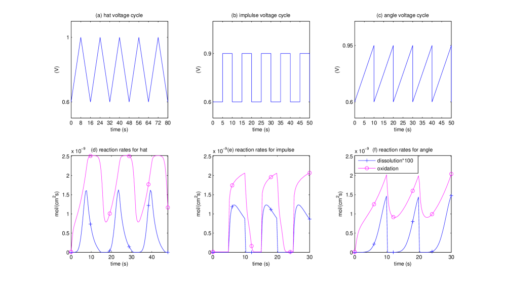
Figure 3: The $\Lambda$-shaped (a) and $\Pi$-shaped (b) $\angle$-shaped (c) profiles of cyclic voltage $V(t)$. The reaction rates $r_{\rm dissol}$ and $r_{\rm oxide}$ for the $\Lambda$ (d), $\Pi$ (e), $\angle$ (f) shaped $V(t)$ within 3 cycles.

Each cycle is characterized by the length $p$. The $\Lambda$-shaped voltage profile is continuous, symmetric, starting and finishing with the minimal voltage value $V_{\rm min}$, attaining the maximal voltage value $V_{\rm max}$ at the half-length $\frac{p}{2}$, thus having the slope $\alpha=\pm\frac{2(V_{\rm max}-V_{\rm min})}{p}$. In the plot (a) in Figure 3, $p=16$ (s), $V_{\rm min}=0.6$ (V), $V_{\rm max}=1$ (V), $\alpha=\pm 5\cdot 10^{-2}$ (V/S). The $\Pi$-shaped voltage profile is discontinuous, characterized by the minimal $V_{\rm min}=0.6$ (V) and the maximal $V_{\rm max}=0.9$ (V) voltages switching at $\frac{p}{2}$ given in Figure 3 (b) for $p=10$ (s). The $\angle$-shaped voltage profile first accelerates during $p=10$ (s) with the slope $\alpha=3.5\cdot 10^{-2}$ (V/S) from the minimal $V_{\rm min}=0.6$ (V) to the maximal $V_{\rm max}=0.95$ (V) voltages and then switches to $V_{\rm min}$ again, see Figure 3 (c).

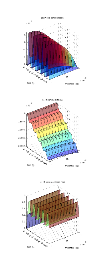
Figure 4: The solution $c$ in (a), $d$ in (b), $\theta$ in (c) under the $\Lambda$-shaped voltage cycle at $T=353.15$ (K).

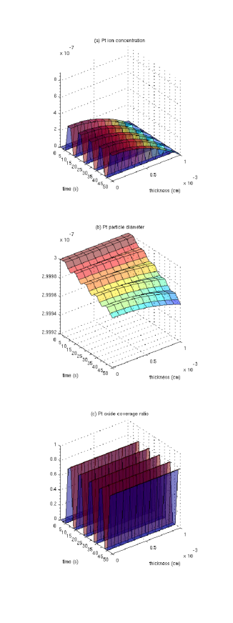
Figure 5: The solution $c$ in (a), $d$ in (b), $\theta$ in (c) under the $\Pi$-shaped voltage cycle at $T=353.15$ (K).

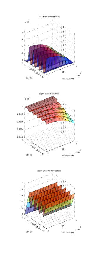
Figure 6: The solution $c$ in (a), $d$ in (b), $\theta$ in (c) under the $\angle$-shaped voltage cycle at $T=353.15$ (K).

In Figure 3 (d), (e), (f) we plot the mean over $x\in[0,L]$ in CL of the reaction rates $r_{\rm dissol}$ scaled by multiplying by 100, and $r_{\rm oxide}$ for the corresponding $\Lambda$, $\Pi$, $\angle$-shaped voltage profiles $V(t)$ within 3 periodic cycles.

We use the numerical model (6) for computer simulation of the catalyst coverage and the CL operation under the $\Lambda$-shaped, $\Pi$-shaped, and $\angle$-shaped voltage cycles taken from Figure 3 (a), (b), and (c). The respective solution triples $(c,d,\theta)$ are depicted in Figure 4, 5, 6 at the temperature $T=80{}^{\circ}$C.

From Figures 4, 5, 6 (a) we observe that at $\Lambda$-shaped voltage cycle the concentration of platinum ions is varied from 0 to around $8\times 10^{-7}$ mol/l; at $\Pi$-shaped voltage cycle the Pt²⁺ increases maximum to $2.3\times 10^{-7}$ mol/l, and at $\angle$-shaped voltage profile it grows until $4\times 10^{-7}$ mol/l. Figures 4, 5, 6 (b) demonstrate the evolution in Pt size distribution through the catalyst length. The Pt size goes down faster at $\Lambda$-shaped voltage cycle than at other two cycles. We should mention, that for all three investigated voltage cycles the Pt particle diameter decreases slightly faster at the membrane surface than at the boundary with the gas diffusion layer. The changes in the coverage of Pt surface by platinum oxide during the voltage cycling are depicted in Figures 4, 5, 6 (c). In $\Lambda$-shaped and $\angle$-shaped voltage cycles, the part of Pt surface is permanently covered by PtO. The ratio of the coverage depends on the voltage. At $\Lambda$-shaped voltage cycle, the PtO coverage is varied from 42 to 82%, while at $\angle$-shaped voltage cycle changes from 30 to 70%. During the $\Pi$-shaped voltage cycle, the platinum oxide covers from 0 to 70% of Pt surface. In this cycle, at the high voltage (0.9 V) the formation of PtO occurs and in the next 5 sec, at the low voltage (0.6 V) the reverse reaction proceeds: the platinum oxide is reduced to the platinum. As seen, at $\Pi$-shaped voltage cycle it is enough time for the reduction reaction, while in other two cycles it does not.

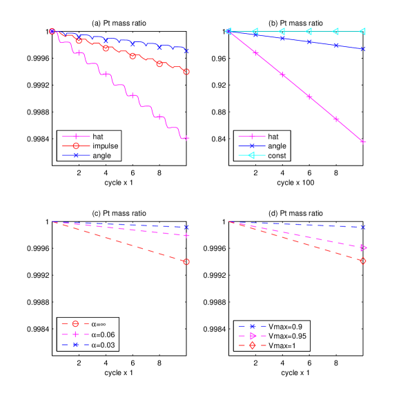
Figure 7: The mean Pt mass loss ration $m_{\rm Pt}$ under various voltage cycles at $T=353.15$ (K).

In Figure 7 we plot the calculated in time steps $l$ platinum mass ratio (the mean over $x\in[0,L]$ in CL):

$$m^{l}_{\rm Pt}=\frac{4}{3}\pi(d^{l})^{3}/V_{\rm Pt}\in[0,1],$$

versus the number of cycles. For comparison, the three curves $m^{l}_{\rm Pt}$ are shown corresponding to the voltage profiles of hat ($\Lambda$), impulse ($\Pi$), and angle ($\angle$) shapes at 10 voltage cycles during 2 min. 40 sec. in plot (a). While in plot (b) the Pt loss is presented at 1000 voltage cycles respectively during 4 hours 26 min. 40 sec. There is also depicted $m^{l}_{\rm Pt}$ under the constant voltage $V(t)=0.65$ (V), thus describing idle state. The linear loss of Pt mass during voltage cycles can be clear observed in Figure 7. The results shown here are determined by the specific choice of profiles and by the upper potential level. Indeed, increasing slopes $\alpha=0.03,0.06,\infty$ (V/s) were tested under the fixed upper potential level $V_{\rm max}=0.9$ (V) as presented in plot (c). This confirms that $\Pi$-shaped profile (marked by $\alpha=\infty$) is the most damaging with respect to livetimes (see experimental data in [29] and [30], Fig. 4). On the other side, increasing the upper potential level $V_{\rm max}=0.9,0.95,1$ (V) under the fixed slope $\alpha=0.03$ (V/s) also shortens the lifetime as shown in plot (d) (see the experimental confirmation in [31], Fig. 5(a)).

The degradation phenomenon would be impossible without the diffusion (when setting $D_{\rm Pt}=0$ as in A). In Figure 8 the corresponding Pt mass loss $m^{l}_{\rm Pt}(x)$ versus $x\in[0,L]$ along CL is presented in plots (a), (b), (c) during 10 voltage cycles of $\Lambda$, $\Pi$, $\angle$ profiles. Here we can also observe the most strong degradation phenomenon near the CL-membrane interface at $x=L$ under the Dirichlet boundary condition.

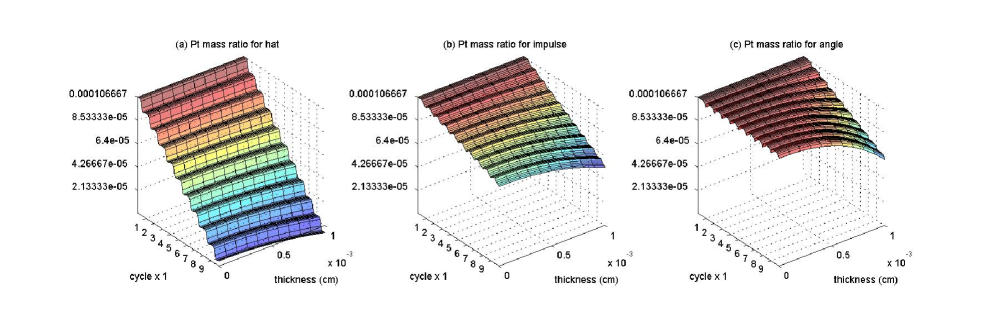
Figure 8: The Pt mass loss ration $m_{\rm Pt}$ vs. CL under $\Lambda$, $\Pi$, $\angle$-shaped voltage cycles at $T=353.15$ (K).

Finally, extrapolating the linear Pt loss based on Figure 7, we calculate the prognosis of the failure when $m_{\rm Pt}$ becomes zero, which is presented in Table 2.

Voltage	Pt mass loss slope	#cycles prognosis	time prognosis
$\Lambda$-shaped	$1.6\times 10^{-4}$	$6\times 10^{3}$	$27$ h
$\Pi$-shaped	$6\times 10^{-5}$	$1.6\times 10^{4}$	$46$ h
$\angle$-shaped	$2.6\times 10^{-5}$	$3.8\times 10^{4}$	$106$ h
constant	$6\times 10^{-8}$	$1.7\times 10^{7}$	$48000$ h

Table 2: The Pt mass loss ration $m_{\rm Pt}$ before failure under various voltage cycles at $T=353.15$ (K).

The average voltages in the studied cycles are 0.8 V for $\Lambda$-shaped cycle; 0.75 V for $\Pi$-shaped and 0.775 V for $\angle$-shaped cycle.

5 Discussion

At present, the degradation effects of Pt/C catalyst in PEMFCs have been extensively studied as experimentally and theoretically. Currently, the decrease in the electroactivity of the Pt/C catalyst has been related with the following mechanisms: 1) Pt dissolution and diffusion into the ionomer; 2) formation of platinum oxides on the Pt particles surface; 3) Pt particle ripening; 4) coalescence of Pt particles. The changes in the electrochemical activities of the catalyst are usually detected using cycling voltammetry or by measuring polarization curves.

In our study we consider only two first degradation mechanisms of Pt and analyze the Pt mass loss and coverage ratio of Pt particle surface by PtO. The simulation presented in the paper is difficult to validate with experimental data available in scientific literature. However, we found some experimental facts confirming the present calculation. For example, Takei et all. [32] investigated Pt degradation of carbon supported Pt catalyst in a single fuel cell as a function of the holding times of OCV/load (square voltage cycling) at $T=80{}^{\circ}$C and RH 100%. Higher operating potential enhanced the Pt oxidation, accelerated the Pt particle growth but suppressed the Pt dissolution. The formation of Pt oxide protects the Pt particle from dissolution.

Ferreira et al. [33] studied a platinum degradation for a short-stack of PEMFC operated at high voltages. Using transmission electron microscopy (TEM) they analyzed a cross-section of MEA cathode samples and determined relative weight percentages of platinum particles on the carbon support as a function of cathode thickness. The analysis showed that the weight percentage of platinum remaining on carbon decreases with increasing distance from gas diffusion layer. After the FC operation the weight percentages of Pt at the interface PEM/CL was twice time lower than at the interface CL/GDL. Yu et al. [26] detected 80% depletion of Pt at cathode/membrane interface after accelerated stress test which was performed by imposing a triangular wave potential cycling from 0.6 V to 1.0 V for 30.000 cycles at 50 mV/sec scan rate. These finding confirm our simulation results indicating that the decrease in Pt weight at the membrane interface same higher than at the interface to GDL.

6 Conclusion

We suggested an one-dimensional and dynamic model which describes degradation phenomena in Pt catalyst of a polymer electrolyte fuel cell such. The model considers Pt dissolution, oxidation as well as diffusion of platinum ions through ionomer of the catalyst layer into the membrane. Also it takes into account an effect of temperature, Pt particle size and Gibbs–Thomson’s effect: dependence of a surface potential on nano-particle size as well as influence of the surface potential on the potential gradient in the system. The developed model is applied to study concentration profile of Pt²⁺ through catalyst length, changes in Pt particle size and mass loss, the coverage ratio of Pt surface by platinum oxide at three different voltage cycles often used in accelerated stress tests: $\Lambda$-shaped, $\Pi$-shaped, and $\angle$-shaped voltage profiles.

For the parameter values from Table 1, we report here on some of our theoretical and numerical findings with respect to admissible voltage operating conditions.

• In order to preserve the physical constraints (2), the sufficient are $V\in[0.6,1]$ (V) for the accelerated $\Lambda$ and $\angle$-shaped voltage cycles, and $V\in[0.6,0.9]$ (V) for the impulse $\Pi$-shaped voltage cycle.

• In Figures 4, 5, and 6 we observe diffusion of the Pt ion concentration $c$ and the Pt particle diameter $d$, whereas a non-diffusive behavior of the Pt coverage ratio $\theta$.

• The reaction rates are shown in Figure 8 for fixed variables, and in Figure 3 during the CL operation.

• The rate of the loss of Pt total mass during voltage cycles depends on the voltage profile and the upper potential level (see Figure 7 and Figure 8, and its prognosis in Table 2).

The study shows that the degradation rate increases with temperature and decreasing particle diameter of Pt nano-particles. The mass loss in platinum and decrease in Pt particle diameter are more significant at the membrane surface than at gas diffusion layer.

Acknowledgments

L. K.-J. is supported by the Austrian Research Promotion Agency (FFG) and the Austrian Ministry for Transport, Innovation and Technology (BMVIT).
V. A. K. is supported by the Austrian Science Fund (FWF) project P26147-N26: PION and the European Research Council (ERC) under European Union’s Horizon 2020 Research and Innovation Programme (advanced grant No. 668998 OCLOC), he thanks the Russian Foundation for Basic Research (RFBR) project 18-29-10007 for partial support.

Appendix A Non-diffusive case

The non-diffusive case of (5) is described by the following system of nonlinear reaction equations: find a triple $c(t)\geq 0$, $d(t)\geq 0$, $0\leq\theta(t)\leq 1$ such that

$${\textstyle\frac{{\rm d}c}{{\rm d}t}}=B_{3}d^{2}\bigl{(}B_{1}(d,\theta)e^{(1-\beta_{1})B_{4}(d,\theta)V}-cB_{2}(d,\theta)e^{-\beta_{1}B_{4}(d,\theta)V}\bigr{)}\quad\text{for $t>0$},$$ (7a)

$${\textstyle\frac{{\rm d}d}{{\rm d}t}}=-\mathit{\Omega}\bigl{(}B_{1}(d,\theta)e^{(1-\beta_{1})B_{4}(d,\theta)V}-cB_{2}(d,\theta)e^{-\beta_{1}B_{4}(d,\theta)V}\bigr{)}\quad\text{for $t>0$},$$ (7b)

$${\textstyle\frac{{\rm d}\theta}{{\rm d}t}}+{\textstyle\frac{2\theta}{d}}{\textstyle\frac{{\rm d}d}{{\rm d}t}}={\textstyle\frac{r_{\rm oxide}(\theta)}{\mathit{\Gamma}}}\quad\text{for $t>0$},$$ (7c)

which is endowed with the initial conditions:

$$c(0)=0,\quad d(0)=d_{\rm Pt},\quad\theta(0)=0.$$ (7d)

In equations (7a) and (7b), the expression (3a) was inserted in $r_{\rm dissol}$.

Multiplying (7a) with $\mathit{\Omega}$ and (7b) with $B_{3}d^{2}$, after summation we obtain the homogeneous ordinary differential equations (ODE):

$${\textstyle\frac{{\rm d}}{{\rm d}t}}\bigl{(}\mathit{\Omega}c+{\textstyle\frac{B_{3}}{3}}d^{3}\bigr{)}=0\quad\text{for $t>0$},$$

which implies the first integral of the system

$$c(t)=c(0)+{\textstyle\frac{B_{3}}{3\mathit{\Omega}}}d^{3}(0)-{\textstyle\frac{B_{3}}{3\mathit{\Omega}}}d^{3}(t).$$ (8)

With the help of (8), the system (7a)–(7c) can be reduced to two equations for either $c$ and $\theta$, or $d$ and $\theta$.

We note also the following special cases. Dividing (7c) with $\theta\not=0$ implies the ODE:

$${\textstyle\frac{{\rm d}}{{\rm d}t}}\bigl{(}\ln(\theta d^{2})\bigr{)}={\textstyle\frac{r_{\rm oxide}(\theta)}{\mathit{\Gamma}\theta}}\quad\text{for $t>0$}.$$ (9)

If the Pt oxidation reaction rate is $r_{\rm oxide}(\theta)\equiv 0$ (the equilibrium state), then the equation (9) is solved trivially as

$$\theta(t)={\textstyle\frac{\theta(0)}{d^{2}(t)}}d^{2}(0)\equiv 0$$

due to the initial conditions (7d).

On the other side, if $\theta(t)\equiv 1$ then $B_{1}(d,1)=B_{2}(d,1)=0$ in (3b). Henceforth, the equations (7a) and (7b) have zero right-hand sides and possess the constant solutions $c(t)\equiv c(0)=0$ and $d(t)\equiv d(0)=d_{\rm Pt}$.

Appendix B Analytical solution

We assume that the Pt particle diameter $d$ and PtO coverage ratio $\theta$ are constant in time, hence the coefficients $B_{1}$, $B_{2}$, and $B_{4}$ are constant, and (7) is reduced to the following Cauchy problem for a single linear inhomogeneous ODE:

$${\textstyle\frac{{\rm d}c}{{\rm d}t}}(t)=B_{1}B_{3}d^{2}e^{(1-\beta_{1})B_{4}V(t)}-c(t)B_{2}B_{3}d^{2}e^{-\beta_{1}B_{4}V(t)}\quad\text{for $t>0$},$$ (10a)

$$c(0)=0.$$ (10b)

In the following we solve (10) analytically for non-steady state voltage $V(t)$.

We introduce an auxiliary function $K(t)$ such that (10a) can be rewritten equivalently as the following system for $t>0$:

$${\textstyle\frac{{\rm d}K}{{\rm d}t}}(t)=B_{2}B_{3}d^{2}K(t)e^{-\beta_{1}B_{4}V(t)},$$ (11a)

$${\textstyle\frac{{\rm d}(Kc)}{{\rm d}t}}(t)=K{\textstyle\frac{{\rm d}c}{{\rm d}t}}(t)+c{\textstyle\frac{{\rm d}K}{{\rm d}t}}(t)=B_{1}B_{3}d^{2}K(t)e^{(1-\beta_{1})B_{4}V(t)}.$$ (11b)

The integration of the equations (11a) and (11b), respectively,

$$K(t)=K(0)e^{B_{2}B_{3}d^{2}\int_{0}^{t}e^{-\beta_{1}B_{4}V(s)}\,{\rm d}s},$$ (12a)

$$(Kc)(t)=(Kc)(0)+B_{1}B_{3}d^{2}\int_{0}^{t}e^{(1-\beta_{1})B_{4}V(\tau)}K(\tau)\,{\rm d}\tau,$$ (12b)

and the subsequent substitution of (12a) into (12b) leads to the explicit expression

$$c(t)=e^{-B_{2}B_{3}d^{2}\int_{0}^{t}e^{-\beta_{1}B_{4}V(s)}\,{\rm d}s}\bigl{(}c(0)\\ +B_{1}B_{3}d^{2}\int_{0}^{t}e^{(1-\beta_{1})B_{4}V(\tau)+B_{2}B_{3}d^{2}\int_{0}^{\tau}e^{-\beta_{1}B_{4}V(s)}\,{\rm d}s}\,{\rm d}\tau\bigr{)},$$ (13)

which can be shortened using the homogeneous initial condition (10b).

References

- [1] M. Eikerling, A. Kulikovsky, Polymer Electrolyte Fuel Cells, Elsevier, Amsterdam, 2017.
- [2] L. Karpenko-Jereb, T. Araki, Modeling of polymer electrolyte fuel cells, in: V. Hacker, S. Mitsushima (Eds.), Fuel Cells and Hydrogen, Elsevier, Amsterdam, 2018, Ch. 3, pp. 41–62. doi:10.1016/B978-0-12-811459-9.00003-7.
- [3] B. Sørensen, G. Spazzafumo, Hydrogen and Fuel Cells, Elsevier, Amsterdam, 2018.
- [4] J.-H. Wee, Applications of proton exchange membrane fuel cell systems, Renew. Sust. Energ. Rev. 11 (8) (2007) 1720–1738. doi:10.1016/j.rser.2006.01.005.
- [5] L. Karpenko-Jereb, C. Sternig, C. Fink, R. Tatschl, Membrane degradation model for 3D CFD analysis of fuel cell performance as a function of time, Int. J. Hydrogen Energ. 41 (31) (2016) 13644–13656. doi:10.1016/j.ijhydene.2016.05.229.
- [6] A. Kulikovsky, T. Berg, Positioning of a reference electrode in a pem fuel cell, J. Electrochem. Soc. 162 (8) (2015) F843–F848. doi:10.1149/2.0231508jes.
- [7] Z. Zheng, F. Yang, C. Lin, F. Zhu, S. Shen, G. Wei, J. Zhang, Design of gradient cathode catalyst layer (CCL) structure for mitigating Pt degradation in proton exchange membrane fuel cells (PEMFCs) using mathematical method, J. Power Sources 451 (2020) 227729. doi:10.1016/j.jpowsour.2020.227729.
- [8] J. Zhang, B. Litteer, W. Gu, H. Liu, H. Gasteiger, Effect of hydrogen and oxygen partial pressure on Pt precipitation within the membrane of PEMFCs, J. Electrochem. Soc. 154 (10) (2007) B1006–B1011. doi:10.1149/1.2764240.
- [9] W. Bi, T. Fuller, Modeling of PEM fuel cell Pt/C catalyst degradation, J. Power Sources 178 (2008) 188–196. doi:10.1016/j.jpowsour.2007.12.007.
- [10] E. Holby, W. Sheng, Y. Shao-Horn, D. Morgan, Pt nanoparticle stability in PEM fuel cells: influence of particle size distribution and crossover hydrogen, Energy Environ. Sci. 2 (8) (2009) 865–871. doi:10.1039/B821622N.
- [11] F. Hiraoka, Y. Kohno, K. Matsuzawa, S. Mitsushima, A simulation study of Pt particle degradation during potential cycling using a dissolution/deposition model, Electrocatalysis 6 (1) (2015) 102–108. doi:10.1007/s12678-014-0225-y.
- [12] Y. Li, K. Moriyama, W. Gu, S. Arisetty, C. Wang, A one-dimensional Pt degradation model for polymer electrolyte fuel cells, J. Electrochem. Soc. 162 (8) (2015) F834–F842. doi:10.1149/2.0101508jes.
- [13] A. Baricci, M. Bonanomi, H. Yu, L. Guetaz, R. Maric, A. Casalegno, Modelling analysis of low platinum polymer fuel cell degradation under voltage cycling: Gradient catalyst layers with improved durability, J. Power Sources 405 (2018) 89–100. doi:10.1016/j.jpowsour.2018.09.092.
- [14] E. Koltsiva, V. Vasilenko, A. Shcherbakov, E. Fokina, V. Bogdanovskaya, Mathematical simulation of PEMFC platinum cathode degradation accounting catalyst’s nanoparticles growth, Chem. Eng. Trans. 70 (2018) 1303–1308. doi:10.3303/CET1870218.
- [15] E. Holby, D. Morgan, Application of Pt nanoparticle dissolution and oxidation modeling to understanding degradation in PEM fuel cells, J. Electrochem. Soc. 159 (5) (2012) B578–B591. doi:10.1149/2.011204jes.
- [16] K. Fellner, V. Kovtunenko, A singularly perturbed nonlinear Poisson–Boltzmann equation: uniform and super-asymptotic expansions, Math. Meth. Appl. Sci. 38 (16) (2015) 3575–3586. doi:10.1002/mma.3593.
- [17] J. González-Granada, V. Kovtunenko, Entropy method for generalized Poisson–Nernst–Planck equations, Anal. Math. Phys. 8 (4) (2018) 603–619. doi:10.1007/s13324-018-0257-1.
- [18] V. Kovtunenko, A. Zubkova, Mathematical modeling of a discontinuous solution of the generalized Poisson–Nernst–Planck problem in a two-phase medium, Kinet. Relat. Mod. 11 (1) (2018) 119–135. doi:10.3934/krm.2018007.
- [19] M. Hintermüller, V. Kovtunenko, K. Kunisch, Constrained optimization for interface cracks in composite materials subject to non-penetration conditions, J. Engrg. Math. 59 (3) (2007) 301–321. doi:10.1007/s10665-006-9113-7.
- [20] H. Itou, V. Kovtunenko, K. Rajagopal, The Boussinesq flat-punch indentation problem within the context of linearized viscoelasticity, Int. J. Eng. Sci. 151. doi:10.1016/j.ijengsci.2020.103272.
- [21] A. Khludnev, V. Kovtunenko, Analysis of Cracks in Solids, Vol. 6 of Int. Ser. Adv. Fract. Mech., WIT-Press, Southampton, Boston, 2000.
- [22] U. Ascher, S. Ruuth, R. Spiteri, Implicit-explicit Runge–Kutta methods for time-dependent partial differential equations, Appl. Numer. Math. 25 (2–3) (1997) 151–167. doi:10.1016/S0168-9274(97)00056-1.
- [23] J. Rumble, CRC Handbook of Chemistry and Physics, CRC Press, Boca Raton, 2019.
- [24] D. Dobos, Electrochemical Data: a Handbook for Electrochemists in Industry and Universities, Elsevier, Amsterdam, 1975.
- [25] S. Burlatsky, M. Gummalla, V. Atrazhev, D. Dmitriev, N. Kuzminyh, N. Erikhman, The dynamics of platinum precipitation in an ion exchange membrane, J. Electrochem. Soc. 158 (3) (2011) B322–B330. doi:10.1149/1.3532956.
- [26] H. Yu, A. Baricci, A. Bisello, A. Casalegno, L. Guetaz, L. Bonville, R. Maric, Strategies to mitigate Pt dissolution in low Pt loading proton exchange membrane fuel cell: I. a gradient Pt particle size design, Electrochim. Acta 247 (2017) 1155–1168. doi:10.1016/j.electacta.2017.07.093.
- [27] P. Urchaga, T. Kadyk, S. Rinaldo, A. Pistono, J. Hu, W. Lee, C. Richards, M. Eikerling, C. Rice, Catalyst degradation in fuel cell electrodes: accelerated stress tests and model-based analysis, Electrochim. Acta 176 (2015) 1500–1510. doi:10.1016/j.electacta.2015.03.152.
- [28] S. Stariha, N. Macauley, B. Sneed, D. Langlois, K. More, R. Mukundan, R. Borup, Recent advances in catalyst accelerated stress tests for polymer electrolyte membrane fuel cells, J. Electrochem. Soc. 165 (7) (2018) F492–F501. doi:10.1149/2.0881807jes.
- [29] M. Uchimura, S. Kocha, The impact of cycle profile on PEMFC durability, ESC Trans. 11 (2007) 215–1226. doi:10.1149/1.2781035.
- [30] A. Kneer, N. Wagner, C. Sadeler, A.-C. Scherzer, D. Gerteisen, Effect of dwell time and scan rate during voltage cycling on catalyst degradation in PEM fuel cells, J. Electrochem. Soc. 165 (10) (2018) F805–F812. doi:10.1149/2.0651810jes.
- [31] A. Kneer, N. Wagner, A semi-empirical catalyst degradation model based on voltage cycling under automotive operating conditions in PEM fuel cells, J. Electrochem. Soc. 166 (2) (2019) F120–F127. doi:10.1149/2.0641902jes.
- [32] C. Takei, K. Kakinuma, K. Kawashima, K. Tashiro, M. Watanabe, M. Uchida, Load cycle durability of a graphitized carbon black-supported platinum catalyst in polymer electrolyte fuel cell cathodes, J. Power Sources 324 (2016) 729–737. doi:10.1016/j.jpowsour.2016.05.117.
- [33] P. Ferreira, G. la O’, Y. Shao-Horn, D. Morgan, R. Makharia, S. Kocha, H. Gasteiger, Instability of Pt/C electrocatalysts in proton exchange membrane fuel cells, J. Electrochem. Soc. 152 (11) (2005) A2256–A2271. doi:10.1149/1.2050347.