Less is More: Surgical Phase Recognition from Timestamp Supervision

Abstract

Surgical phase recognition is a fundamental task in computer-assisted surgery systems. In this paper, we introduce timestamp supervision for surgical phase recognition to train the models with timestamp annotations, where the surgeons are asked to identify only a single timestamp within the temporal boundary of a phase. This annotation can significantly reduce the manual annotation cost compared to the full annotations. To make full use of such timestamp supervisions, we propose a novel method called uncertainty-aware temporal diffusion (UATD) to generate trustworthy pseudo labels for training. Our proposed UATD is motivated by the property of surgical videos, i.e., the phases are long events consisting of consecutive frames. To be specific, UATD diffuses the single labelled timestamp to its corresponding high confident ( i.e., low uncertainty) neighbour frames in an iterative way.

Surgical phase recognition, timestamp supervision, uncertainty estimation

1 Introduction

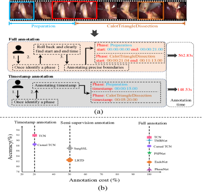
Figure 1: (a)  (b)

Computer-assisted surgery systems can improve the surgery’s quality and ensure the patients’ safety in modern operating rooms [1, 2]. Surgical phase recognition is one key component of computer-assisted surgery systems, which aims to predict which phase is occurring at the current frame [3, 4]. It can be used for automatic indexing of surgical video databases [5], monitoring surgical process [6], scheduling surgeons [7] and assessing surgeons’ skills [8]. In recent years, automated surgical phase recognition has featured deep learning [9, 10, 11] and has reached promising recognition performance [12, 5, 13]. Most current surgical phase recognition approaches require full annotations from surgeons, i.e., the surgeons need to find the precise start and end time for a surgical phase. To this end, the surgeon should repeat watching the video at a very slow speed to find a specific time for the start of the phase. Then, the surgeon needs to continue to watch the video and find the precise end time of the phase. As shown in Fig. 1 (a), this full annotation is very time-consuming, e.g., surgeons need to spend an average of 562.83 seconds to annotate a video. Furthermore, the boundaries between different phases are usually ambiguous [12].

To generate more pseudo labels, some researchers propose to detect the action changes between two consecutive labeled frames for action recognition in natural videos with timestamp supervision [14]. However, this method displays limited performance to surgical videos because surgical videos contain more ambiguous boundaries, leading to the noisy and inconsistent pseudo labels; see Sec. 4.5 for detailed discussion.

To address the above problems, we leverage the the property of surgical videos to generate more trustworthy pseudo labels from timestamp supervision. The property we observed is that phases in the surgical video are long events consisting of continuous frames, which shows a desirable temporal property that the closer the frames to the annotated timestamp, the more likely they are to be classified to the same label as the annotated one. Frames far from the annotated timestamp are difficult to have correct pseudo labels. Based on the above property, a Uncertainty-Aware Temporal Diffusion (UATD) module is proposed to diffuse the annotated timestamps to their adjacent low-uncertainty frames in the temporal axis. In this way, only frames with high confidence and near the annotated timestamps would be considered for adding into pseudo-labels for training.

We conduct empirical studies based on the proposed UATD and LP, and discover important insights of surgical phase recognition from timestamp supervision as follow: 1) Timestamp annotation can reduce $74\%$ annotation time compared with the full annotation, and surgeons tend to annotate those timestamps that are near the middle of phases; see details in Fig. 3. 2) Extensive experiments demonstrate that our method can achieve competitive results compared with full supervision methods, while reducing manual annotation cost; see details in Table 1. 3) Less is more in surgical phase recognition, i.e., less but discriminative pseudo labels outperform full but containing ambiguous frames; see details in -Table. 1. 4) The proposed UATD can be used as a plug and play method to clean ambiguous labels near boundaries between phases, and improve the performance of the current surgical phase recognition methods; see details in Fig 10. The reason is that training with our method would help to decrease intra-class distance and increase inter-class distance simultaneously; see details in Table. 9. The main contributions of this work can be summarized as the following:

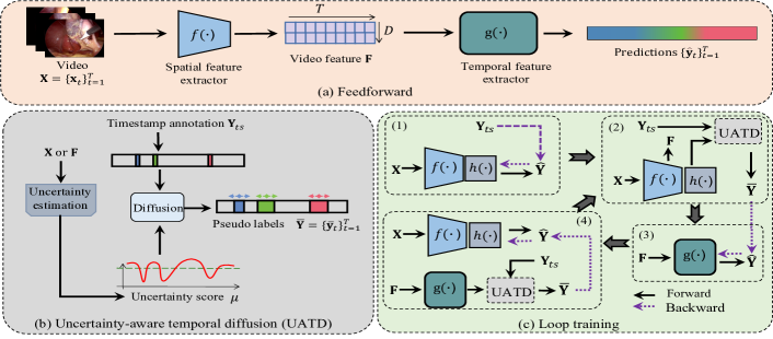
Figure 2:

2 Related Work

2.1 Surgical Phase Recognition

We broadly classified related methods for surgical phase recognition into two categories including fully-supervised learning and label-efficient learning.

Fully-supervised Learning. In fully-supervised learning, each frame in a surgical video is labeled. Early works [16, 17, 18] use hand-crafted features such as color and texture to perform recognition, which achieves limited performance and poor generalization. With the development of neural networks, recent deep learning based methods achieve the great success [5, 3, 19, 20, 15, 4, 21, 22, 13, 12]. EndoNet [5] first uses a convolutional neural network to automatically learn features and prove its effectiveness for surgical phase recognition. SV-RCNet [3] integrates and to learn both spatial and temporal representations in an end-to-end way. To capture the long-range temporal relationship, TMRNet [4] introduces a memory bank and TeCNO [24] uses dilated temporal convolutional network to get a large receptive field. Recently, Yi et al. [20] realize the negative effect of hard frames and propose data cleansing and online hard frames mapper to detect and handle them respectively. Yi et al. [21] find that simply applying multi-stage architecture e.g. multi-stage TCN makes the refinement fall short and thus design not end-to-end training manner to alleviate this problem. Trans-SVNet [13] proposes a hybrid embedding aggregation Transformer to fuse spatial and temporal embedding. Ding et al. [12] emphasize the importance of segment-level semantics and extract semantic-consistent segments to refine the erroneous predictions. Notably, some related methods [5, 24, 15] utilize additional tool presence labels to perform a multi-task learning to facilitate surgical phase recognition.

Semi-supervised Learning. Despite the great success the above methods get, they require a large amount of annotated videos, which is very costly. some researchers [26, 27, 28, 29, 30] explore the methods for semi-supervision, where only parts of videos in the dataset are fully annotated, and others are unlabelled. For example, LRTD [29] use active learning to this context. It captures the long-range temporal dependency among continuous frames in the unlabeled data pool and selects the clips with weak dependencies to annotate. Yengera et al. [27] introduce self-supervised pre-training ensuring all available laparoscopic videos can be utilized. Yu et al. [26] propose a teacher/student approach where the teacher is trained on a small set of labeled videos and generates pseudo labels on the rest of unlabeled videos for student model learning. Furthermore, SurgSSL [30] uses consistency regularization and pseudo labeling to leverage the knowledge in unlabeled data, which progressively leverages the inherent knowledge held in the unlabeled data to a larger extent.

.

2.2 Weak Supervision for Video Understanding

Weakly supervision has received widespread attention in some video understanding tasks, such as temporal action localization [31, 32, 33, 34, 35, 36, 37] and action segmentation [38, 39, 40]. Some of them use video-level supervision, i.e., a set of action categories, while some use transcript-level supervision, i.e., an ordered list of actions. For example, Richard et al. [41] leverage text-based grammar from unordered action sets. Although they significantly reduce the annotation effort, the performance is quite limited. To trade-off the annotation-efficient and performance, timestamp supervision [42, 43, 44, 14] is proposed for action recognition. For example, SF-Net [44] designs an action frame mining and a background frame mining strategy to introduce more negative frames into the training process. However, the above methods aiming at temporal action localization task generate very limited pseudo labels, is not suitable for surgical phase recognition, i.e., frame-wise recognition. In the action segmentation task, to generate frame-wise pseudo labels, Li et al. [14] detect the action change between two consecutive timestamps by stamp-to-stamp energy function and generate full pseudo labels. However, in surgical videos, the frames near boundaries are generally ambiguous, the generated pseudo labels may be noisy annotations, which degrades the performance. Compared with previous approaches, our proposed method generates as many confident pseudo labels as possible by considering the temporal relationships among frames, while discarding pseudo labels with a large uncertainty.

2.3 Uncertainty Estimation

3 Method

3.1 Problem Definition

Let $\mathbf{X}=\{\mathbf{x}_{t}\}_{t=1}^{T}$ be a surgical video with $T$ frames, where is the $t$-th frame. Each surgical video is divided into several phases, and there is no overlapping among phases. Our goal is to learn a spatial feature extractor network $f(\cdot)$ and a temporal feature extractor $g(\cdot)$ that maps the frame $\mathbf{x}_{t}$ to a phase label, which is presented in Fig. 2 (a). In the full supervision, the frame-wise labels $\mathbf{Y}=\{\mathbf{y}_{1},\ldots,\mathbf{y}_{T}\}$ are available. However, in our timestamp supervision, given a video consisting of $N$ phases, where $N<<T$, only a single timestamp in each phase are annotated as $\mathbf{Y}_{ts}=\{\mathbf{y}_{t_{1}},\ldots,\mathbf{y}_{t_{N}}\}$, where $t_{i}$ is in the $i$-th phase, $\mathbf{y}_{t_{i}}\in\{1,2,\ldots,C\}$, and $C$ is the total number of classes.

To perform surgical phase recognition with timestamp supervision, we propose an uncertainty-aware temporal diffusion (UATD) to generate trustworthy pseudo labels, denoted as $\overline{\mathbf{Y}}$, from the timestamp supervision $\mathbf{Y}_{ts}$ to optimize $f(\cdot)$ and $g(\cdot)$. The proposed UATD is shown in Fig. 2 (b); see Sec. 3.2 for details. Furthermore, we introduce the loop training, which optimizes $f(\cdot)$ and $g(\cdot)$ in an iterative way to reduce the memory cost and imbalance optimization; see Fig. 2 (c) and Section 3.3 for details.

3.2 Uncertainty-aware Temporal Diffusion

In timestamp supervision $\mathbf{Y}_{ts}$, i.e., only a single label for each phase, the total number of positive frames is quite small and may be difficult to learn a robust model. Although we do not have full annotations, it is clear that the phases are long events consisting of consecutive frames. Motivated by this property of surgical videos, we propose the uncertainty-aware temporal diffusion (UATD) to diffuse the single labelled frame to its corresponding high confident (i.e., low uncertainty) neighbour frames. In this way, we can introduce more frames acted as pseudo labels into the training process. Furthermore, the diffusion of frames is stopped by low confident frames, which can avoid the ambiguous annotations. The proposed UATD consists two components: uncertainty estimation and temporal diffusion. In the following, we describe the two components respectively.

Temporal diffusion. After obtaining the uncertainty score $\mu_{t}$, we use the temporal diffusion module to diffuse the current labels to more pseudo labels for training in the next iteration; see the iterative training details in Sec. 3.3. To be specific, we treat the labeled frames as anchors and start diffusion from anchors to the adjacent frames on either sides of them in temporal dimension, which is illustrated in Algorithm 1. By the temporal diffusion, one frame would be introduced into next iteration training only if the uncertainty score of it is lower than a threshold $\tau$ and the predicted class label equals to its nearby timestamp frame. In this way, the generated pseudo label would be high confidence, avoid introducing noisy annotations. Note that in the obtained pseudo labels $\overline{\mathbf{Y}}=\{\overline{\mathbf{y}}_{t}\}_{t=1}^{T}$, $\mathbf{y}_{t}=0$ means the $t$-th frame is not labelled.

3.3 Loop Training

Algorithm 2

Input: .
Output:

1:

2:for $i=1$ to $n$ do

3:     $\triangleright$

4:     

5:     $\triangleright$

6:     

7:end for

8:for $j=1$ to $m$ do

9:     

10:     for $i=1$ to $n$ do

11:         $\triangleright$

12:         

13:         $\triangleright$

15:     end for

16:     $\triangleright$

17:     

18:end for

In the loop training, we only sample labelled frames (annotated timestamp or generated pseudo labels) to optimize the spatial feature extractor or temporal feature extractor, which can not be achieved in previous jointly training. Formally, there four main steps in our loop training:

(a) Optimizing the spatial feature extractor: $f(\cdot),h(\cdot)\leftarrow\text{OptimS}(f(\cdot),h(\cdot),\mathbf{X},\overline{\mathbf{Y}},\mathcal{L}_{ce})$. To be specific, the input video $\mathbf{X}$ is fed into the spatial feature extractor $f$ to obtain the video feature $\mathbf{F}=f(\mathbf{X})$. Then a classifier $h(\cdot)$ is used to obtain the prediction $\hat{\mathbf{Y}}=h(\mathbf{F})$, where $\hat{\mathbf{Y}}=\{\hat{\mathbf{y}_{t}}\}_{t=1}^{T}$. Given the target labels (timestamp annotation or pseudo labels) $\overline{\mathbf{Y}}=\{\overline{\mathbf{y}}_{t}\}_{t_{1}}^{T}$, the objective for the spatial feature extractor can be formulated as:

$$\mathcal{L}_{ce}=-\frac{1}{T}\sum_{t=1,\overline{\mathbf{y}}_{t}\neq 0}^{T}\overline{\mathbf{y}}_{t}\log(\hat{\mathbf{y}}_{t}),$$ (4)

where $\overline{\mathbf{y}}_{t}\neq 0$ indicates the $t$-th frame is not labelled.

(b) Extracting the spatial features: $\mathbf{F}=f(\mathbf{X})$; see details in step (1).

(c) Optimizing the temporal feature extractor: $g(\cdot)\leftarrow\text{OptimT}(g(\cdot),\mathbf{F},\overline{\mathbf{Y}},\mathcal{L}_{ce},\mathcal{L}_{smooth})$. Specifically, the video feature $\mathbf{F}$ is fed into $g(\cdot)$ to capture the temporal relation of frames and obtain the corresponding predictions $\hat{\mathbf{Y}}$. We use the CrossEntropy loss to train the $g(\cdot)$, similar as $f(\cdot)$. Compared with the spatial feature extractor, to encourage a smooth transition between frames, we use the truncated mean squared error as a Smoothing Loss following [55, 14]:

$$\mathcal{L}_{smooth}=\frac{1}{TC}\sum_{t,c}\tilde{\Delta}_{t,c}^{2},$$ (5)

$$\tilde{\Delta}_{t,c}^{2}=\left\{\begin{aligned} \Delta_{t,c}^{2}&,&\quad\Delta_{t,c}<\gamma\\ \gamma&,&\quad otherwise\end{aligned}\right.,$$ (6)

$$\Delta_{t,c}=|log({\hat{\bm{y}}_{t,c}})-log(\hat{\bm{y}}_{t-1,c})|,$$ (7)

where $T$ is the video length and $C$ is the number of action classes. This loss function explicitly penalize the difference of each two adjacent frames and we suggest readers refer to [55] for more details. The final loss function is the weighted sum of these two losses:

$$\mathcal{L}=\mathcal{L}_{ce}+\lambda\mathcal{L}_{smooth},$$ (8)

where $\lambda$ is a hyper-parameter to balance the contribution of each loss and is set to $0.015$ for all of our experiments.

After the definiation of the four steps, we illustrate the loop training in Algorithm 2.

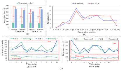
Figure 3:

Table 1: Comparison with the state-of-the-art on Cholec80 and M2CAI16 datasets.

Method	Cholec80				M2CAI16
	AC (%)	PR (%)	RE (%)	JA (%)	AC (%)	PR (%)	RE (%)	JA (%)
Fully Supervised Methods - $\bm{100\%}$ annotation time
PhaseNet [56]	$78.8\pm 4.7$	$71.3\pm 15.6$	$76.6\pm 16.6$	-	$79.5\pm 12.1$	-	-	$64.1\pm 10.3$
EndoNet [5]	$81.7\pm 4.2$	-	$79.6\pm 7.9$	-	-	-	-	-
SV-RCNet [3]	$85.3\pm 7.3$	$80.7\pm 7.0$	$83.5\pm 7.5$	-	$81.7\pm 8.1$	$81.0\pm 8.3$	$81.6\pm 7.2$	$65.4\pm 8.9$
OHFM[20]	$87.3\pm 5.7$	-	-	$67.0\pm 13.3$	$85.2\pm 7.5$	-	-	$68.8\pm 10.5$
Casual TCN [14]	$87.9\pm 8.2$	$86.4\pm 7.7$	$84.8\pm{12.9}$	$72.4\pm{9.4}$	$81.9\pm{11.3}$	$84.8\pm{5.2}$	$82.2\pm{9.0}$	$68.1\pm{8.5}$
TeCNO [24]	$88.6\pm 7.8$	$86.5\pm 7.0$	$88.8\pm 17.4$	$75.1\pm 6.9$	-	-	-	-
TMRNet [4]	$90.1\pm 7.6$	$90.3\pm 3.3$	$89.5\pm 5.0$	$79.1\pm 5.7$	$87.0\pm 8.6$	$87.8\pm 6.9$	$88.4\pm 5.3$	$75.1\pm 6.9$
Trans-SVNet [13]	$90.3\pm 7.1$	$90.7\pm 5.0$	$88.8\pm 7.4$	$79.3\pm 6.6$	$87.2\pm 9.3$	$88.0\pm 6.7$	$87.5\pm 5.5$	$74.7\pm 7.7$
TCN	$91.1\pm{6.7}$	${90.8\pm{4.5}}$	$87.6\pm{11.7}$	$79.1\pm{8.5}$	$82.9\pm{10.8}$	$85.8\pm{5.4}$	$82.7\pm{9.0}$	$69.7\pm{8.7}$
Not end-to-end [21]	$91.5\pm 7.1$	-	$87.2\pm 8.2$	$77.2\pm 11.2$	${88.2\pm 8.5}$	-	${91.4\pm 11.2}$	$75.1\pm 10.6$
Semi Supervised Methods - $\bm{50\%}$ annotation time
LRTD [29]	$82.5\pm 8.4$	$79.7\pm 9.0$	$80.9\pm 8.1$	$64.2\pm 10.2$	$72.1\pm 13.7$	$74.1\pm 14.9$	$74.0\pm 10.4$	$54.4\pm 12.9$
SurgSSL [30]	$87.0\pm 7.4$	$84.2\pm 8.9$	$85.2\pm 11.1$	$70.5\pm 12.6$	$79.6\pm 9.4$	$80.2\pm 11.3$	$79.6\pm 11.5$	$62.0\pm 11.1$
Timestamp Supervised Methods - annotation time
Casual TCN+Ours	$88.6\pm 6.7$	$86.1\pm 6.7$	$88.0\pm 10.1$	$73.7\pm 10.2$	$86.0\pm 7.8$	$85.0\pm 6.2$	$87.1\pm 7.7$	$71.4\pm 10.4$
TCN+Ours	${91.9\pm 5.6}$	$89.5\pm 4.4$	${90.5\pm 5.9}$	${79.9\pm 8.5}$	$87.6\pm 8.7$	${88.2\pm 7.4}$	$87.9\pm 9.6$	${75.7\pm 9.5}$

4 Experiments

4.1 Datasets and Metrics

M2CAI16. The M2CAI16 dataset [57] consists of $41$ laparoscopic videos that are acquired at 25fps of cholecystectomy procedures, and each frame has a resolution of 1920$\times$1080. Following  [21], $27$ videos are used for training while the rest $14$ are used for testing. These videos are segmented into $8$ phases by experienced surgeons.

Cholec80. The cholec80 dataset [5] contains $80$ videos of cholecystectomy surgeries performed by $13$ surgeons. All the videos are recorded at $25$ fps, and the frames in them have the resolution of $1920\times 1080$ or $854\times 480$. The dataset is divided into two subsets of equal size, with the first $40$ videos as a training set and the other $40$ as a testing set.

Evaluation metrics. Following previous works [3, 4, 5, 20], we utilize four metrics, i.e., accuracy (AC), precision (PR), recall (RE), and Jaccard (JA), to evaluate the phase prediction accuracy. Among them, accuracy and Jaccard index are used to evaluate the submission of M2CAI Workflow Challenge, while precision and recall are also commonly used metrics for video-based phase recognition.

4.2

4.3 Implementation Details

Our code is based on PyTorch using an NVIDIA GeForce RTX 3090 GPU. We downsample the video to 1fps for training in all experiments following previous works [5, 3, 4]. All the frames are resized to a resolution of $250\times 250$, and data augmentations including $224\times 224$ cropping, random mirroring, and color jittering are applied during the training stage. We get a pre-trained inception-v3 [58] on ImageNet [59]. The batch size is set to $8$, and an Adam optimizer with an initial learning rate of $1e-4$ and weight decay of $1e-5$ is used. We further use a step learning rate scheduler where the step size is two epochs and decay rate is $0.5$ for fune-tuning by $5$ epochs. To train TCN, we use Adam optimizer with an initial learning rate of $1e-3$ and cosine annealing for learning rate decay. For all experiments, we set a dropout rate of $0.5$ and an uncertainty threshold $\tau=0.1$; the detailed analysis is shown in Table 4. The uncertainty is estimated by $5$ forward times Monte Carlo Dropout. [46]. The numbers of rounds of uncertainty-aware temporal diffusion and loop training are set to $m=4$ and $n=2$, respectively. Furthermore, the timestamp annotations are simulated by randomly selecting one frame from each action phase in the training videos.

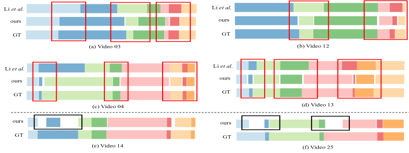
Figure 4:

4.4 Comparison with the State-of-the-Arts

We compare our less is more method with the state-of-the-arts on the Cholec80 and M2CAI16 datasets, and report their results in Table 1. It is clear that our method outperforms previous data-efficient methods, i.e., semi-supervised ones, on both data efficiency and phase recognition performance. For example, our timestamp supervision only requires annotation time of the full supervision [44], while semi-supervision needs $50\%$ annotation time [29]. Moreover, our method with the casual TCN [14] achieves $88.6\%$ of accuracy on Cholec80 dataset, achieving the compared to semi-supervised methods. We can also find that our method can even achieve the competitive performance compared with the fully supervised methods, with only annotation time of them. Notably, the improvements of our method are more significant in M2CAI16 than in Cholec80. This is because M2CAI16 contains more ambiguous frames [12], which degrades the performance. The details why our methods can outperform corresponding backbones in fully supervised setup will be discussed in Sec. 4.6.

Table 2: Comparison with different timestamp supervision methods.

Method	AC (%)	PR (%)	RE (%)	JA (%)
Cholec80
Naive
Uniform
Li et al.[14]
Ours
M2CAI16
Naive
Uniform
Li et al.[14]
Ours

4.5 Comparison with Different Timestamp Supervision Methods

To evaluate the efficiency of our proposed uncertainty-aware temporal diffusion (UATD) for surgical video timestamp supervision, we compare our methods with two baseline models following [14], i.e., Naive and Uniform, and report the results in Table 2. It is clear that our method outperforms other two methods with a clear margin. Furthermore, we also compare Li et al. [14], which is the SOTA in action segmentation under this setting. It uses the middle output of model i.e., features of frames to detect action change and generate frame-wise pseudo labels However, using feature similarity to detect action change could be confused when the boundaries are generally ambiguous. As shown in Fig. 4, our methods give accurate pseudo labels by stopping diffusion near boundaries while [14] attempts to give unappealing labels. From Table. 2, we can also see that our method obtains $7\%-13\%$ improvements over all metrics.

Table 3: Ablative study of key components on Cholec80 dataset. ‘UATD (S)’ and ‘UATD (T)’ indicate using UATD in the spatial feature and temporal feature extractors. ‘LP’ indicates the loop training which is defined in Sec. 3.3.

UATD (S)	UATD (T)	LP	AC (%)	PR (%)	RE (%)	JA (%)
✗	✗	✗
✔	✗	✗
✗	✔	✗
✗	✗	✔
✔	✔	✗
✔	✔	✔

Table 4: Quantitative results of different uncertainty thresholds.

	AC (%)	PR (%)	RE (%)	JA (%)	Labelling	Labelling
					Rate (%)	Accuracy (%)
$\tau=\infty$	$84.65$	$86.34$	$84.65$	$70.43$	$\bm{93.49}$	$92.04$
$\tau=0.2$	$85.32$	$\bm{86.71}$	$85.06$	$71.14$	$92.72$	$94.13$
$\tau=0.1$	$\bm{85.95}$	$84.96$	$\bm{87.05}$	$\bm{71.43}$	$87.51$	$96.99$
$\tau=0.05$	$85.49$	$86.19$	$86.42$	$71.20$	$60.76$	$\bm{99.04}$

Table 5:

Iteration	TS	1-st	2-nd	3-rd
Labelling Rate (%)	0.33	67.70	76.82	84.45
Labelling Accuracy (%)	100.00	98.69	97.95	97.42

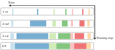
Figure 5:

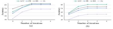
Figure 6:

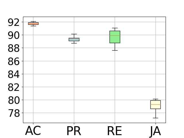
(a) Cholec80

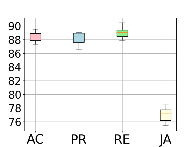
(b) M2CAI16

Figure 7: Box plots of performance of random timestamp annotations on Cholec80 and M2CAI16 datasets.

Table 6: Quantitative results of Start, End, Middle and Random timestamp positions on Cholec80 dataset.

Timestamp	AC (%)	PR (%)	RE (%)	JA (%)
Position
Start	$90.64$	$87.92$	$88.37$	$76.75$
End	$90.17$	$88.35$	$82.24$	$70.75$
Middle	$\bm{92.59}$	$\bm{90.13}$	$\bm{89.60}$	$\bm{80.04}$
Random	$91.86$	$89.51$	$90.52$	$79.90$

Table 7: Comparison of annotation time between a single timestamp and two timestamps.

Video Index	01	05
Single Timestamp	222s	155s
Two Timestamps	331s	279s

Table 8:

Method	Annotation	AC (%)	PR (%)	RE (%)	JA (%)

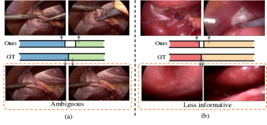
Figure 8:

4.6 Ablation Study

Effect of UATD and LP. There are two key components, i.e., uncertainty-aware temporal diffusion (UATD) and loop training (LP), in our method. We ablate the effect of them in Table. 3. It is clear that the proposed UATD can improve the timestamp supervision with a clear margin, e.g., combined with UATD, the model achieves $85.59\%$ accuracy, outperforming $18.67\%$ over the baseline model. Also, we could find that loop training contributes to around $3\%$ improvements.

Impact of the uncertainty threshold $\tau$. The quality of pseudo labels is depended on pseudo labeling rate and pseudo labels accuracy, which is controlled by the uncertainty threshold $\tau$ in Algorithm 1. In order to evaluate the effect of $\tau$, we compare the performance of the models with different $\tau$ and report the results in Table 4. We can find that the higher uncertainty threshold would lead to the higher pseudo labeling rate and the lower accuracy of pseudo labels, and vice versa. For example, with infinity threshold, i.e., first row in Table 4, pseudo labeling rate can reach $93.49\%$ while accuracy of pseudo labels is only $92.04\%$. Such higher labeling rate would introduce more noisy labels, which degrades the labeling accuracy. In our paper, we set $\tau$ to $0.1$ for the best trade-off.

Given only a single manual labeled annotations, we show that our model can generate more and more reliable pseudo-labels step by step in Table 5. “Labelling Rate” and “Labelling Accuracy” are the same meaning as Table 4. It shows that our method can generate more and more pseudo labels the number of iterations increases. This is because each iteration of temporal diffusion gives temporal model extra information, the model can generate more pseudo labels next time. Also, the accuracy of generated pseudo labels is very trustworthy. Since the frames show very similar appearances to their adjacent frames, the network can easily generate correct predictions for the neighbor frames of the annotated frame. We also show the visualization of the

In our experiments, the timestamp annotations are generated by randomly selecting one frames to be annotated of each phase. The short and flat boxes indicate that our proposed method is robust to different timestamp annotations, What’s more, our method can outperform most of methods in Table. 1 with even the worst timestamp annotations.

As shown in Table. 6, annotating at the start and end frames of each phase would degrade the performance. This is because that frames near boundaries are generally ambiguous, which can be hard to act as an anchor of temporal diffusion. In the contrast, the middle frames are more discriminative to represent current phases and thus can generate more correct pseudo labels. Actually, the surgeons ,i.e., the annotators, tend to label the discriminative frames because they can easily recognize them when seeing through the whole video [44], which ensure timestamp annotations efficient and effective.

During the timestamp annotation, once a phase is identified and current timestamp is recorded, the surgeon could choose to record another timestamp for the phase. Here, we compare the annotation cost between a single and two timestamps in Table 7. Two videos, i.e.,“01” and “05”, are sampled from Cholec80 and M2CAI16 respectively. The result shows that two timestamp annotation would cost more time than a single timestamp annotation, e.g., the surgeon would spend $331$s for “01” while annotating a single timestamp only requires $222$s. We also conduct experiments to compare the performance of the models training with a single timestamp and two timestamps, as shown in Table 8. The results show that two timestamp annotation cannot achieve clear improvement but bring additional annotation cost. Hence, annotating a single timestamp is much efficient than two timestamps, and we use the best efficient way to solve surgical phase recognition in this paper.

Comparison of generated pseudo label and ground-truth. In our experiments, we find that our method only generates pseudo labels for discriminative frames while ignores the ambiguous ones near boundaries. As shown in Fig. 8, our generated pseudo labels discard ambiguous or frames compared to the ground-truth. More importantly, the model trained with our generated pseudo labels outperforms the model trained with the ground-truth; see details in Table. 1.

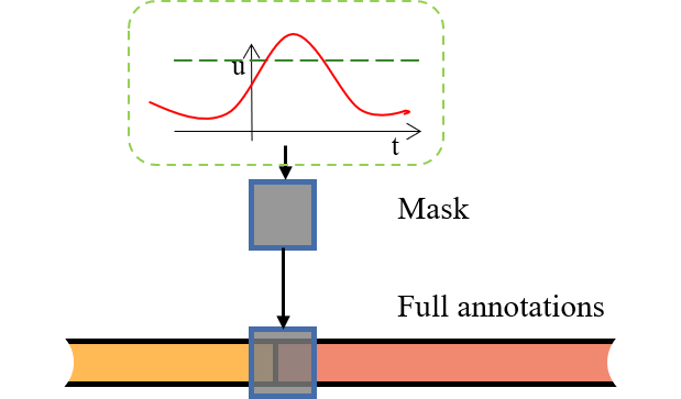
(a) Ours

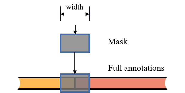
(b) Fixed width

Figure 9: (a) Masking boundaries by using UATD to detect ambiguous frames. (b) Masking boundaries by fixed width.

Table 9: ‘Timestamp’ is using our generated pseudo labels by UATD from timestamp annotations and ‘GT w/ UATD’ indicates the ground-truth labels masked by UATD; see Sec. 4.7 for details.

Method	Annotation	AC (%)	PR (%)	RE (%)	JA (%)
Casual TCN	GT	$87.94$	$86.40$	$84.81$	$72.40$
	Timestamp	$88.56$	$86.05$	$88.00$	$73.72$
	GT w/ UATD	$\bm{91.18}$	$\bm{89.88}$	$\bm{90.93}$	$\bm{79.76}$
TCN	GT	$91.14$	$90.84$	$87.64$	$79.14$
	Timestamp	$91.86$	$89.51$	$90.52$	$79.90$
	GT w/ UATD	$\bm{92.75}$	$\bm{91.23}$	$\bm{93.10}$	$\bm{83.89}$

Table 10: Effectiveness of boundary mask on Cholec80 dataset.

Mask width	AC (%)	PR (%)	RE (%)	JA (%)
0	$91.14$	$90.84$	$87.64$	$79.14$
3	$92.04$	$91.87$	$89.07$	$81.44$
5	$92.31$	$92.26$	$89.52$	$82.12$
10	$\bm{92.75}$	$92.86$	$\bm{90.57}$	$\bm{83.32}$
20	$92.68$	$\bm{93.20}$	$90.40$	$82.66$

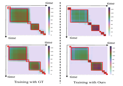
Figure 10:

4.7 Incorporate UATD into Current Methods

As analyzed in Fig. 8, we find that our method can only generate labels for discriminative frames, instead of ambiguous frames. To this end, as shown in Fig. 9 (a), we mask some ground-truth labels near boundaries, based on the pseudo labels generated by our methods. To be specific, we use UATD to generate pseudo labels, and record the indexes of unlabelled frames that are with high uncertainty. Then, we remove those frames with the recorded indexes from the ground-truth, and obtained a clean ground-truth to supervise the model. We compare the performance of the models training with (a) , (b) pseudo labels generated by UATD and GT masked by UATD, and report the results in Table 9. , it is clear that the model training with GT masked by UATD can achieve the best results, even outperforms the current SOTA; see Table 1 for comparison. We further conduct experiments on the models training with GT masked by the fixed width, as shown in Fig. 9 (b). As illustrated in Table. 10, masking some frames near boundary during training outperform the model without masking over around $1\%-3\%$ in all metrics. However, it will introduce a new hyper-parameter, i.e., the width of mask, which is critical to the performance. Hence, in order to achieve the good performance, we need to conduct many experiments to find the best choice, which is very time-consuming. On the contrary, our method can be used as an approach to clean the noisy labels in the ground-truth automatically, without the need of hand-designed width. To further explain this phenomenon, we visualize the feature similarity matrix in Fig. 10. Each red box in each similarity matrix indicates each phase in a video. It is clear that training with our generate pseudo labels i.e., removing ambiguous labels near boundaries between two phases, would help to decrease intra-class distance and increase inter-class distance simultaneously.

5 Discussion

Surgical phase recognition is one key component of computer-assisted surgery systems, which advances context-awareness in modern operating rooms. However, most existing works require full annotations which are expensive, expertise-required and error-prone [28]. In contrast, we introduce timestamp supervision which only requires one timestamp annotated by human for each phase in a video. We invite two surgeons to conduct both full and timestamp annotations and record the time cost for these two annotations. To leverage this supervision, we propose Uncertainty-Aware Temporal Diffusion (UATD) to generate trustworthy pseudo labels for those unlabeled frames, which is based on the property of surgical phases. Furthermore, loop training is also introduce to address the imbalance training and memory cost in timestamp surgical phase recognition. The in-depth empirical studies of the proposed UATD and LP based on timestamp supervision discovers four deep insights: 1) Timestamp annotation can reduce $74\%$ annotation time compared with the full annotation, and surgeons tend to annotate those timestamps that are near the middle of phases; 2) Extensive experiments demonstrate that our method can achieve competitive results compared with full supervision methods, while reducing manual annotation cost; 3) Less is more in surgical phase recognition, i.e., less but discriminative pseudo labels outperform full but containing ambiguous frames; 4) The proposed UATD can be used as a plug and play method to clean ambiguous labels near boundaries between phases, and improve the performance of the current surgical phase recognition methods; see details in Table 9.

Although our method achieves promising results, there are some limitations. First, the temporal property we consider is not overall yet. The diffusion in our method assumes that the workflow is smooth without dramatic change and hardly any ambiguous frame occurs in the internal of phase . But such assumption may be false for other datasets and in the future we will study more comprehensive temporal relationship to handle the intra-phase discontinuity. Moreover, the training process we propose is time-consuming containing several iterations of training model from scratch. And we will design more elegant training process to link up the optimal learning from different annotations, i.e., different rounds of temporal diffusion in our methods.

Finally, we expect community to focus more on label-efficient surgical video analysis. The weakly setting of videos, such as transcripts [39] and timestamp supervision, deserve further attention and exploiting. And the related ideas can be further investigated in other medical image analysis problems in CT [61, 62, 63, 64], MRI [65, 66, 67].

6 Conclusion

In this paper, we introduce the most annotation-saving setting, namely timestamp supervision, for surgical phase recognition. With timestamp supervision, we propose a novel uncertainty-aware temporal diffusion (UATD) method to generate trustworthy pseudo labels according to the labeled frames. Our main idea is to generate pseudo labels by considering the relationship among video frames. Results on two datasets show that our method can achieve the competitive performance compared with the fully supervised setup. Moreover, we also find that our method can be used as a labeling clean approach to remove the noisy labels near boundaries to improve the generalization of the current surgical phase recognition, which reveals an interesting phenomenon less is more in this task. This paper provides some insights for label-efficient surgical phase recognition and hopefully inspire researchers to design label-efficient surgical video analysis algorithms.

References

- [1] L. Maier-Hein, S. S. Vedula, S. Speidel, N. Navab, R. Kikinis, A. Park, M. Eisenmann, H. Feussner, G. Forestier, S. Giannarou, et al., “Surgical data science for next-generation interventions,” Nature Biomedical Engineering, vol. 1, no. 9, pp. 691–696, 2017.
- [2] A. Moglia, V. Ferrari, L. Morelli, M. Ferrari, F. Mosca, and A. Cuschieri, “A systematic review of virtual reality simulators for robot-assisted surgery,” European urology, vol. 69, no. 6, pp. 1065–1080, 2016.
- [3] Y. Jin, Q. Dou, H. Chen, L. Yu, J. Qin, C.-W. Fu, and P.-A. Heng, “Sv-rcnet: workflow recognition from surgical videos using recurrent convolutional network,” IEEE transactions on medical imaging, vol. 37, no. 5, pp. 1114–1126, 2017.
- [4] Y. Jin, Y. Long, C. Chen, Z. Zhao, Q. Dou, and P.-A. Heng, “Temporal memory relation network for workflow recognition from surgical video,” IEEE Transactions on Medical Imaging, 2021.
- [5] A. P. Twinanda, S. Shehata, D. Mutter, J. Marescaux, M. De Mathelin, and N. Padoy, “Endonet: a deep architecture for recognition tasks on laparoscopic videos,” IEEE transactions on medical imaging, vol. 36, no. 1, pp. 86–97, 2016.
- [6] N. Bricon-Souf and C. R. Newman, “Context awareness in health care: A review,” international journal of medical informatics, vol. 76, no. 1, pp. 2–12, 2007.
- [7] B. Bhatia, T. Oates, Y. Xiao, and P. Hu, “Real-time identification of operating room state from video,” in AAAI, vol. 2, pp. 1761–1766, 2007.
- [8] D. Liu, Q. Li, T. Jiang, Y. Wang, R. Miao, F. Shan, and Z. Li, “Towards unified surgical skill assessment,” in Proceedings of the IEEE/CVF Conference on Computer Vision and Pattern Recognition, pp. 9522–9531, 2021.
- [9] K. He, X. Zhang, S. Ren, and J. Sun, “Deep residual learning for image recognition,” in Proceedings of the IEEE conference on computer vision and pattern recognition, pp. 770–778, 2016.
- [10] K. Simonyan and A. Zisserman, “Very deep convolutional networks for large-scale image recognition,” arXiv preprint arXiv:1409.1556, 2014.
- [11] Z. Liu, Y. Lin, Y. Cao, H. Hu, Y. Wei, Z. Zhang, S. Lin, and B. Guo, “Swin transformer: Hierarchical vision transformer using shifted windows,” arXiv preprint arXiv:2103.14030, 2021.
- [12] X. Ding and X. Li, “Exploring segment-level semantics for online phase recognition from surgical videos,” IEEE Transactions on Medical Imaging, 2022.
- [13] X. Gao, Y. Jin, Y. Long, Q. Dou, and P.-A. Heng, “Trans-svnet: Accurate phase recognition from surgical videos via hybrid embedding aggregation transformer,” arXiv preprint arXiv:2103.09712, 2021.
- [14] Z. Li, Y. Abu Farha, and J. Gall, “Temporal action segmentation from timestamp supervision,” in Proceedings of the IEEE/CVF Conference on Computer Vision and Pattern Recognition, pp. 8365–8374, 2021.
- [15] Y. Jin, H. Li, Q. Dou, H. Chen, J. Qin, C.-W. Fu, and P.-A. Heng, “Multi-task recurrent convolutional network with correlation loss for surgical video analysis,” Medical image analysis, vol. 59, p. 101572, 2020.
- [16] T. Blum, H. Feußner, and N. Navab, “Modeling and segmentation of surgical workflow from laparoscopic video,” in International Conference on Medical Image Computing and Computer-Assisted Intervention, pp. 400–407, Springer, 2010.
- [17] F. Lalys, L. Riffaud, D. Bouget, and P. Jannin, “A framework for the recognition of high-level surgical tasks from video images for cataract surgeries,” IEEE Transactions on Biomedical Engineering, vol. 59, no. 4, pp. 966–976, 2011.
- [18] A. Graves, “Practical variational inference for neural networks,” Advances in neural information processing systems, vol. 24, 2011.
- [19] I. Funke, S. Bodenstedt, F. Oehme, F. von Bechtolsheim, J. Weitz, and S. Speidel, “Using 3d convolutional neural networks to learn spatiotemporal features for automatic surgical gesture recognition in video,” in International Conference on Medical Image Computing and Computer-Assisted Intervention, pp. 467–475, Springer, 2019.
- [20] F. Yi and T. Jiang, “Hard frame detection and online mapping for surgical phase recognition,” in International Conference on Medical Image Computing and Computer-Assisted Intervention, pp. 449–457, Springer, 2019.
- [21] F. Yi and T. Jiang, “Not end-to-end: Explore multi-stage architecture for online surgical phase recognition,” arXiv preprint arXiv:2107.04810, 2021.
- [22] B. Zhang, A. Ghanem, A. Simes, H. Choi, A. Yoo, and A. Min, “Swnet: Surgical workflow recognition with deep convolutional network,” in Medical Imaging with Deep Learning, 2021.
- [23] M. Sahu, A. Szengel, A. Mukhopadhyay, and S. Zachow, “Surgical phase recognition by learning phase transitions,” Current Directions in Biomedical Engineering, vol. 6, no. 1, 2020.
- [24] T. Czempiel, M. Paschali, M. Keicher, W. Simson, H. Feussner, S. T. Kim, and N. Navab, “Tecno: Surgical phase recognition with multi-stage temporal convolutional networks,” in International Conference on Medical Image Computing and Computer-Assisted Intervention, pp. 343–352, Springer, 2020.
- [25] T. Czempiel, M. Paschali, D. Ostler, S. T. Kim, B. Busam, and N. Navab, “Opera: Attention-regularized transformers for surgical phase recognition,” in International Conference on Medical Image Computing and Computer-Assisted Intervention, pp. 604–614, Springer, 2021.
- [26] T. Yu, D. Mutter, J. Marescaux, and N. Padoy, “Learning from a tiny dataset of manual annotations: a teacher/student approach for surgical phase recognition,” arXiv preprint arXiv:1812.00033, 2018.
- [27] G. Yengera, D. Mutter, J. Marescaux, and N. Padoy, “Less is more: Surgical phase recognition with less annotations through self-supervised pre-training of cnn-lstm networks,” arXiv preprint arXiv:1805.08569, 2018.
- [28] R. DiPietro and G. D. Hager, “Automated surgical activity recognition with one labeled sequence,” in International conference on medical image computing and computer-assisted intervention, pp. 458–466, Springer, 2019.
- [29] X. Shi, Y. Jin, Q. Dou, and P.-A. Heng, “Lrtd: long-range temporal dependency based active learning for surgical workflow recognition,” International Journal of Computer Assisted Radiology and Surgery, vol. 15, no. 9, pp. 1573–1584, 2020.
- [30] X. Shi, Y. Jin, Q. Dou, and P.-A. Heng, “Semi-supervised learning with progressive unlabeled data excavation for label-efficient surgical workflow recognition,” Medical Image Analysis, vol. 73, p. 102158, 2021.
- [31] K. K. Singh and Y. J. Lee, “Hide-and-seek: Forcing a network to be meticulous for weakly-supervised object and action localization,” in 2017 IEEE international conference on computer vision (ICCV), pp. 3544–3553, IEEE, 2017.
- [32] L. Wang, Y. Xiong, D. Lin, and L. Van Gool, “Untrimmednets for weakly supervised action recognition and detection,” in Proceedings of the IEEE conference on Computer Vision and Pattern Recognition, pp. 4325–4334, 2017.
- [33] P. Nguyen, T. Liu, G. Prasad, and B. Han, “Weakly supervised action localization by sparse temporal pooling network,” in Proceedings of the IEEE Conference on Computer Vision and Pattern Recognition, pp. 6752–6761, 2018.
- [34] S. Paul, S. Roy, and A. K. Roy-Chowdhury, “W-talc: Weakly-supervised temporal activity localization and classification,” in Proceedings of the European Conference on Computer Vision (ECCV), pp. 563–579, 2018.
- [35] X. Ding, N. Wang, X. Gao, J. Li, X. Wang, and T. Liu, “Weakly supervised temporal action localization with segment-level labels,” arXiv preprint arXiv:2007.01598, 2020.
- [36] X. Ding, N. Wang, X. Gao, J. Li, X. Wang, and T. Liu, “Kfc: An efficient framework for semi-supervised temporal action localization,” IEEE Transactions on Image Processing, vol. 30, pp. 6869–6878, 2021.
- [37] X. Ding, N. Wang, S. Zhang, D. Cheng, X. Li, Z. Huang, M. Tang, and X. Gao, “Support-set based cross-supervision for video grounding,” in Proceedings of the IEEE/CVF International Conference on Computer Vision, pp. 11573–11582, 2021.
- [38] P. Bojanowski, R. Lajugie, F. Bach, I. Laptev, J. Ponce, C. Schmid, and J. Sivic, “Weakly supervised action labeling in videos under ordering constraints,” in European Conference on Computer Vision, pp. 628–643, Springer, 2014.
- [39] D.-A. Huang, L. Fei-Fei, and J. C. Niebles, “Connectionist temporal modeling for weakly supervised action labeling,” in European Conference on Computer Vision, pp. 137–153, Springer, 2016.
- [40] J. Li, P. Lei, and S. Todorovic, “Weakly supervised energy-based learning for action segmentation,” in Proceedings of the IEEE/CVF International Conference on Computer Vision, pp. 6243–6251, 2019.
- [41] A. Richard, H. Kuehne, and J. Gall, “Action sets: Weakly supervised action segmentation without ordering constraints,” in Proceedings of the IEEE conference on Computer Vision and Pattern Recognition, pp. 5987–5996, 2018.
- [42] P. Mettes, J. C. Van Gemert, and C. G. Snoek, “Spot on: Action localization from pointly-supervised proposals,” in European conference on computer vision, pp. 437–453, Springer, 2016.
- [43] D. Moltisanti, S. Fidler, and D. Damen, “Action recognition from single timestamp supervision in untrimmed videos,” in Proceedings of the IEEE/CVF Conference on Computer Vision and Pattern Recognition, pp. 9915–9924, 2019.
- [44] F. Ma, L. Zhu, Y. Yang, S. Zha, G. Kundu, M. Feiszli, and Z. Shou, “Sf-net: Single-frame supervision for temporal action localization,” in European conference on computer vision, pp. 420–437, Springer, 2020.
- [45] A. Kendall and Y. Gal, “What uncertainties do we need in bayesian deep learning for computer vision?,” arXiv preprint arXiv:1703.04977, 2017.
- [46] Y. Gal and Z. Ghahramani, “Dropout as a bayesian approximation: Representing model uncertainty in deep learning,” in international conference on machine learning, pp. 1050–1059, PMLR, 2016.
- [47] B. Lakshminarayanan, A. Pritzel, and C. Blundell, “Simple and scalable predictive uncertainty estimation using deep ensembles,” Advances in neural information processing systems, vol. 30, 2017.
- [48] R. Tanno, D. E. Worrall, A. Ghosh, E. Kaden, S. N. Sotiropoulos, A. Criminisi, and D. C. Alexander, “Bayesian image quality transfer with cnns: exploring uncertainty in dmri super-resolution,” in International Conference on Medical Image Computing and Computer-Assisted Intervention, pp. 611–619, Springer, 2017.
- [49] A. Jungo, F. Balsiger, and M. Reyes, “Analyzing the quality and challenges of uncertainty estimations for brain tumor segmentation,” Frontiers in neuroscience, p. 282, 2020.
- [50] D. P. Kingma and M. Welling, “Auto-encoding variational bayes,” arXiv preprint arXiv:1312.6114, 2013.
- [51] K. Sohn, H. Lee, and X. Yan, “Learning structured output representation using deep conditional generative models,” Advances in neural information processing systems, vol. 28, 2015.
- [52] M.-H. Laves, S. Ihler, and T. Ortmaier, “Uncertainty quantification in computer-aided diagnosis: Make your model say” i don’t know” for ambiguous cases,” arXiv preprint arXiv:1908.00792, 2019.
- [53] C. Leibig, V. Allken, M. S. Ayhan, P. Berens, and S. Wahl, “Leveraging uncertainty information from deep neural networks for disease detection,” Scientific reports, vol. 7, no. 1, pp. 1–14, 2017.
- [54] G. Wang, W. Li, M. Aertsen, J. Deprest, S. Ourselin, and T. Vercauteren, “Aleatoric uncertainty estimation with test-time augmentation for medical image segmentation with convolutional neural networks,” Neurocomputing, vol. 338, pp. 34–45, 2019.
- [55] Y. A. Farha and J. Gall, “Ms-tcn: Multi-stage temporal convolutional network for action segmentation,” in Proceedings of the IEEE/CVF Conference on Computer Vision and Pattern Recognition, pp. 3575–3584, 2019.
- [56] A. P. Twinanda, D. Mutter, J. Marescaux, M. de Mathelin, and N. Padoy, “Single-and multi-task architectures for surgical workflow challenge at m2cai 2016,” arXiv preprint arXiv:1610.08844, 2016.
- [57] A. Twinanda, S. Shehata, D. Mutter, J. Marescaux, M. De Mathelin, and N. Padoy, “Miccai modeling and monitoring of computer assisted interventions challenge,” 2016.
- [58] C. Szegedy, V. Vanhoucke, S. Ioffe, J. Shlens, and Z. Wojna, “Rethinking the inception architecture for computer vision,” in Proceedings of the IEEE conference on computer vision and pattern recognition, pp. 2818–2826, 2016.
- [59] A. Krizhevsky, I. Sutskever, and G. E. Hinton, “Imagenet classification with deep convolutional neural networks,” Advances in neural information processing systems, vol. 25, pp. 1097–1105, 2012.
- [60] N. Ahmidi, L. Tao, S. Sefati, Y. Gao, C. Lea, B. B. Haro, L. Zappella, S. Khudanpur, R. Vidal, and G. D. Hager, “A dataset and benchmarks for segmentation and recognition of gestures in robotic surgery,” IEEE Transactions on Biomedical Engineering, vol. 64, no. 9, pp. 2025–2041, 2017.
- [61] X. Li, H. Chen, X. Qi, Q. Dou, C.-W. Fu, and P.-A. Heng, “H-denseunet: hybrid densely connected unet for liver and tumor segmentation from ct volumes,” IEEE transactions on medical imaging, vol. 37, no. 12, pp. 2663–2674, 2018.
- [62] E. Gibson, F. Giganti, Y. Hu, E. Bonmati, S. Bandula, K. Gurusamy, B. Davidson, S. P. Pereira, M. J. Clarkson, and D. C. Barratt, “Automatic multi-organ segmentation on abdominal ct with dense v-networks,” IEEE transactions on medical imaging, vol. 37, no. 8, pp. 1822–1834, 2018.
- [63] T. Heimann, B. Van Ginneken, M. A. Styner, Y. Arzhaeva, V. Aurich, C. Bauer, A. Beck, C. Becker, R. Beichel, G. Bekes, et al., “Comparison and evaluation of methods for liver segmentation from ct datasets,” IEEE transactions on medical imaging, vol. 28, no. 8, pp. 1251–1265, 2009.
- [64] X. Li, L. Yu, H. Chen, C.-W. Fu, L. Xing, and P.-A. Heng, “Transformation-consistent self-ensembling model for semisupervised medical image segmentation,” IEEE Transactions on Neural Networks and Learning Systems, vol. 32, no. 2, pp. 523–534, 2020.
- [65] T. Wang, X. Xu, J. Xiong, Q. Jia, H. Yuan, M. Huang, J. Zhuang, and Y. Shi, “Ica-unet: Ica inspired statistical unet for real-time 3d cardiac cine mri segmentation,” in International conference on medical image computing and computer-assisted intervention, pp. 447–457, Springer, 2020.
- [66] X. Li, Q. Dou, H. Chen, C.-W. Fu, X. Qi, D. L. Belavỳ, G. Armbrecht, D. Felsenberg, G. Zheng, and P.-A. Heng, “3d multi-scale fcn with random modality voxel dropout learning for intervertebral disc localization and segmentation from multi-modality mr images,” Medical image analysis, vol. 45, pp. 41–54, 2018.
- [67] Y. Yu, Y. Xie, T. Thamm, E. Gong, J. Ouyang, C. Huang, S. Christensen, M. P. Marks, M. G. Lansberg, G. W. Albers, et al., “Use of deep learning to predict final ischemic stroke lesions from initial magnetic resonance imaging,” JAMA network open, vol. 3, no. 3, pp. e200772–e200772, 2020.