Modelling multi-cell edge video analytics

Abstract

Edge intelligence is a scalable solution for analyzing distributed data, but it cannot provide reliable services in large-scale cellular networks unless the inherent aspects of fading and interference are also taken into consideration. In this paper, we present the first mathematical framework for modelling edge video analytics in multi-cell cellular systems. We derive the expressions for the coverage probability, the ergodic capacity, the probability of successfully completing the video analytics within a target delay requirement, and the effective frame rate. We also analyze the effect of the system parameters on the accuracy of the detection algorithm, the supported frame rate at the edge server, and the system fairness.

I Introduction

The evolution of mobile devices has introduced tremendous innovation opportunities for developing new services beyond personal communications. These advances have brought new mobile applications, and with them, the proliferation of large amounts of app-level data. At the same time, we have experienced major breakthroughs in deep learning, which have made it possible to manage and leverage the rise in data volumes for solving complex problems, such as image classification, language processing, or intrusion detection [1].

However, as we strive for more accurate and reliable deep learning models, the computationally and energy-constrained mobile devices make real-time processing intractable. One prominent solution to extend the capabilities of mobile devices is to offload the computationally intensive tasks to an edge computing server. Edge computing offers a distributed solution that brings the computational resources closer to the mobile devices, and provides lower latency, more energy efficiency, better privacy protection, and lesser bandwidth consumption than its counterpart cloud-based infrastructure [2]. Edge computing also makes it easier to gather richer data and learn from the behaviour of nearby mobile devices, making it possible to explore deep learning models for interactive cloud gaming, cognitive assistance, and real-time video analytics [2].

Indeed, the growing interest in both edge computing and artificial intelligence has coined the term edge intelligence. This area of research is however in its early stages, and most of the proposed solutions are optimized to be deployed on local networks, such that it can be assumed that all users have similar network conditions and similar probabilities of successfully completing their task. In large-scale cellular networks, aspects of noise, fading, or interference can significantly impact the wireless communication [3], so those assumptions no longer hold, and analyzing the communication between the mobile users and the edge server becomes as relevant as analyzing the implementation of the deep learning models. Hence, there needs to be a tractable approach to understand how the network, the computing resources, and the deep learning models affect altogether the task offloading problem.

In this work, we present a mathematical framework for analyzing edge-intelligent, multi-cell cellular systems supporting video analytics. We specifically leverage the tools of stochastic geometry, queuing theory, and deep learning for modelling the entire offloading process under different accuracy-latency constraints. We provide a thorough analysis of the relationship between the parameters of the video analytics, the uplink transmission, the edge server, and the deep learning algorithm, and evaluate their trade-offs via numerical results. Overall, our discussions and results provide the first steps towards designing efficient resource-allocation strategies and traffic-control protocols for edge-intelligent, multi-cell cellular systems.

The remainder of this paper is organized as follows. Section II reviews the related work. Section III describes the system model for the entire offloading process. In Section IV, we derive the expressions for the performance metrics that evaluate the trade-offs between the different parameters in the system. Then, we provide the numerical results in Section V, followed by the concluding remarks in Section VI.

II Related work

Edge intelligence is a promising solution to assist mobile devices with computationally-intensive and latency-stringent applications, and it is recently receiving a lot of attention for visual-aid services, e.g., augmented reality [4] and video edge analytics [5]. As a response to these emerging interests, recent works have built proof-of-concept testbeds [4, 5, 6]. DARE [4] focuses on the edge server and analyzes the effect of the frame size, the frame rate, and the deep learning model on the task offloading problem. DeepDecision [5] considers the same parameters but instead focuses on the mobile users and the wireless network. The work in [6] uses its own measurements to design data-driven statistical models for real-time inference.

The results from the above works highlight the suitability of edge intelligence for improving the accuracy and latency of visual-aid services, but their simplified models for the communication between the mobile users and the edge servers do not capture the inherent aspects of large-scale cellular networks. In this context, [7] models the performance of edge-intelligent systems with parallel processing for video analytics, and [8] models the performance of edge computing in multi-cell networks, but does not address the performance of the application itself.

Our work extends the above results and presents a mathematical framework for analyzing how the conditions of the network, the frame size, and the latency requirements affect the transmission rate, the achievable frame rate, the probability of successfully completing the video analytics, and the accuracy of the detection algorithm.

III System model

III-A Network

Consider a multi-cell wireless network where all the base stations employ frequency-division multiple access with reuse factor $\delta$, such that mobile users experience inter-cell interference but no intra-cell interference. Each mobile user connects to the base station that provides the maximum received power averaged over fading, and each base station has only one active user in a given frequency band, which is arbitrarily chosen from all the mobile users located in its Voronoi cell. Motivated by [9], the locations of the base stations are modelled according to a two-dimensional homogeneous Poisson point process (PPP) with intensity $\lambda_{b}$. Similarly, the locations of the mobile users using the same frequency resources are considered to be independent and modelled according to some other stationary PPP with intensity $\lambda_{u}$. Considering this, it can be shown that the distance between any user and its serving base station, denoted by $r$, is Rayleigh distributed. The proof follows from the null probability of a two-dimensional PPP [10],

$$\mathcal{P}[R>r]=\mathcal{P}\left[\text{no BS in a circle of area }\pi r^{2}\right]=e^{-\lambda_{b}\pi r^{2}},$$

from which the probability density function (PDF) is

$$f_{R}(r)=2\lambda_{b}\pi r\,e^{-\lambda_{b}\pi r^{2}},\quad r\geq 0.$$ (1)

For the rest of the paper, we consider a target user $k$ and its serving base station, and refer to the set of interfering mobile users as $\mathcal{Z}$. We denote the distances from the interfering users $z\in\mathcal{Z}$ to the base station of interest by $d_{z}$, and the distances from the interfering users to their serving base stations by $r_{z}$. Note that the distances $\{r_{z}\}_{z\in\mathcal{Z}}$ are identically distributed but not necessarily independent. The dependence comes from the structure of the Poisson-Voronoi tessellation and the restriction that there is only one active user in each frequency band. However, [11] shows that this dependence is weak and the distances $\{r_{z}\}_{z\in\mathcal{Z}}$ can be assumed to be independent and identically distributed (i.i.d.). Furthermore, the marginal distribution of $r_{z}$ can be assumed to be Rayleigh distributed as in (1), which is motivated by the irregular deployment of base stations and the same null-probability argument as for $r$.

III-B Uplink transmission

In edge video analytics, the amount of data transmitted in the uplink, i.e., from the users to the base stations, is much larger than the amount of data transmitted in the downlink. Therefore, we focus on modelling the uplink transmission.

We consider that the transmitted signals attenuate with path-loss exponent $\alpha>2$ and experience i.i.d. Rayleigh fading. All the users utilize a maximum-ratio transmission precoding vector, such that the effect of the channel can be modelled at the receiver by the multiplicative Exponential random variable $|g|^{2}\sim\exp(1)$. We define the largest possible time-frequency space within which the effect of the channel can be modelled as a scalar multiplication by $|g|^{2}$ as the coherence interval. We denote the coherence interval by $\tau_{c}=T_{coh}\,B_{coh}$, where $T_{coh}$ represents the coherence time, and $B_{coh}$ represents coherence bandwidth. Considering this, we define the number of coherence intervals that fit into a time-frequency block of $t$ seconds and $B$ Hertz as $N_{\textit{coh}}=t\,B/\tau_{c}$.

Moreover, we consider that all mobile users utilize distance-proportional fractional power control of the form $r^{\alpha\epsilon}$, where $\epsilon\in[0,1]$ is the power control factor. We define a reference power at a distance of $1$ kilometer from the base station as $P$ and assume it to be the same for all the users. To model the maximum transmission power of the mobile users, we consider the transmit powers $Pr^{\alpha\epsilon}$ to be limited by the peak power $\bar{P}$. Finally, we consider the noise power at the receiver to be $\sigma^{2}$. Under this transmission model, the signal-to-interference-noise ratio (SINR) for any randomly selected user $k$ at its serving base station is

$$\text{SINR}_{k}=\frac{|g_{k}|^{2}\,\ell(r,\alpha,\epsilon)\,r^{-\alpha}}{\sigma^{2}_{k}+\sum_{z\in\mathcal{Z}}|g_{z}|^{2}\,\ell(r_{z},\alpha,\epsilon)\,d_{z}^{-\alpha}},$$ (2)

where

$$\ell(r,\alpha,\epsilon)=\min\left(Pr^{\alpha\epsilon},\bar{P}\right),$$ (3)

and the sub-indices $k$ and $z$ indicate if a variable depends on the location and the resources assigned to the target user $k$ or to the interfering users $z\in\mathcal{Z}$, respectively.

For the uplink transmission, we consider that each base station assigns a fixed bandwidth $B_{k}$ to every active user within its Voronoi cell. Once a user $k$ has been assigned a frequency band, it estimates the state of the channel in each coherence interval from pilot signals and adjusts its coding and modulation according to its instantaneous SINR_k. As a result, the transmission rate $R_{k}$ is a random variable that depends on the user’s location, the conditions of the channel, and the inter-cell interference.

III-C Mobile edge computing server

All the base stations in the network are equipped with an independent mobile edge computing server that is responsible for serving all the video analytic users within the Voronoi cell of its corresponding base station. For our base station of interest, we consider that there is a set of $K$ active video analytic users, denoted by $k$, for $k=1,\dots,K$, that are capable of continuously recording images and sending them over the wireless channel. Once the images of these users are completely received at the base station, they are delivered to the server without delay and queued at an infinite buffer for being processed on a first-come-first-served basis.

From the point of view of the server, each user $k$ is seen as an independent entity that offloads images to the server at an arrival rate of $\lambda_{k}$ frames per second. Altogether, since the communication system employs frequency-division multiple access, the queue at the server observes the superposition of $K$ independent arrival processes with an aggregate arrival rate of $\lambda=\sum_{k}\lambda_{k}$ frames per second. Under these assumptions, the arrival process behaves as a Poisson process [12]. Once in queue, the images are processed at the server in a deterministic amount of time $T_{s}$, which is determined by the resolution of the transmitted images and the neural network considered for the video analytics.

In this paper, we consider for simplicity that all the users within the same cell transmit images of the same resolution and perform the video analytics utilizing the same neural network. Hence, it yields that the queuing system at the server can be modelled as an M/D/1 queue with load $\rho=\lambda T_{s}$.

III-D Video analytics

All the servers in the network incorporate an object detection algorithm consisting of a pre-trained YOLOv5 neural network. We specifically consider YOLOv5 [13] for the video analytics because it is capable of handling images of different resolutions without changing its associated learnable parameters, thus making it possible to parametrize the inference time and the accuracy of the detection algorithm.

Following the results in [14], the number of instructions that are required to process an image with a resolution of $s_{k}^{2}$ pixels can be expressed as a convex function of $s_{k}$,

$$f(s_{k})=c_{1}s_{k}^{3}+c_{2},$$ (4)

for some positive constants $c_{1}$ and $c_{2}$, where the units of $f(s_{k})$ are number of floating-point operations (in trillions). Similarly, the accuracy of the detection algorithm can be expressed as a concave function of $s_{k}$,

$$A(s_{k})=c_{3}-c_{4}e^{-c_{5}s_{k}},$$ (5)

for some other positive constants $c_{3}$, $c_{4}$, and $c_{5}$, where the accuracy of the detection is measured as the mean average precision of the object detection algorithm for a predefined threshold of the intersection over union [14]. For more information about the effect of the learning and inference processes on the constants $c_{1},\dots,c_{5}$, please refer to [15].

Moreover, all the computing servers in the network are equipped with a CPU of $h$ TFLOPs. With that, it follows from (4) that the time to process an image of resolution $s_{k}^{2}$ is

$$T_{s,k}=\frac{f(s_{k})}{h}=\frac{c_{1}s_{k}^{3}+c_{2}}{h}.$$ (6)

Note that images of high resolution take longer to process but they result in higher detection accuracies, with a nonlinear trade-off between the processing time and the accuracy of the detection algorithm.

III-E Offloading process

Altogether, the offloading process from beginning to end can be described as follows. All active video analytics users are assigned some frequency resources and are considered to transmit with high priority, that is, they always get access to the wireless channel as soon as they want to offload their images. The transmitted images are considered to be squared with a resolution of $s_{k}^{2}$ pixels, encoded at $\theta$ bits per pixel and compressed at rate $\xi$:1, so an image of $s_{k}^{2}$ pixels is represented by $\theta s_{k}^{2}/\xi$ bits. Once the images are completely received at the serving base station, the images are queued at the edge server and processed one by one by a convolutional neural network. For each user $k$, we denote the time to transmit an image as $T_{ul,k}$, the time spent in the queue as $T_{w,k}$, and the time to process an image as $T_{s,k}$. We refer to the sum of these three times as the delay of the entire offloading process, disregarding the little time of eventual feedback to the user, and let each user $k$ specify a maximum value $t_{k}$ for that delay. For simplicity, we assume that the maximum delay $t_{k}$ is the same for all the users within the same cell.

IV System analysis

IV-A Coverage probability

The coverage probability for any user $k$ in the network is the probability that its uplink SINR_k is greater than some threshold $\gamma_{k}$. Considering this, the coverage probability conditioned to user $k$ being at a fixed distance $r$ from its serving base station can be derived from [11, Theorem 1], for any reuse factor $\delta$ [16, Theorem 4], and power-limit constraint (3) as

$$\mathcal{P}(\text{SINR}_{k}\geq\gamma_{k}|r)$$

$$\;=\mathcal{P}\left(|g_{k}|^{2}\geq\frac{\gamma_{k}\,(\sigma_{k}^{2}+\sum_{z\in\mathcal{Z}}|g_{z}|^{2}\,\ell(r_{z},\alpha,\epsilon)\,d_{z}^{-\alpha})}{\ell(r,\alpha,\epsilon)\,r^{-\alpha}}\bigg{|}r\right)$$

$$\;\overset{(a)}{=}e^{-\frac{\gamma_{k}\,r^{\alpha}}{\ell(r,\alpha,\epsilon)}\,\sigma^{2}_{k}}\;\mathbb{E}\left[\exp\left(-\frac{\gamma_{k}\,\sum_{z\in\mathcal{Z}}|g_{z}|^{2}\,\ell(r_{z},\alpha,\epsilon)\,d_{z}^{-\alpha}}{\ell(r,\alpha,\epsilon)\,r^{-\alpha}}\right)\right]$$

$$\;\overset{(b)}{=}e^{-\frac{\gamma_{k}\,r^{\alpha}}{\ell(r,\alpha,\epsilon)}\,\sigma^{2}_{k}}\mathcal{L}_{I_{z}}\left(\frac{\gamma_{k}\,r^{\alpha}}{\ell(r,\alpha,\epsilon)}\right),$$ (7)

where $(a)$ follows from the exponential distribution of $|g_{k}|^{2}$, and $(b)$ follows from the definition of the Laplace transform of the interference at the serving base station. This Laplace transform can be calculated from the i.i.d. distributions of $r_{z}$ and $d_{z}$, and the Probability Generating Function [10] of the PPP that models the location of the mobile users, such that

$$\mathcal{L}_{I_{z}}(s)=\exp\left(-2\pi\lambda_{u}\int_{r}^{\infty}\beta(x,s)\,x\,dx\right),$$ (8)

with

$$\beta(x,s)=1-\int_{0}^{\infty}\frac{\pi\lambda_{u}\,e^{-\pi\lambda_{u}u}}{1+s\,\ell\left(u^{\frac{1}{2}},\alpha,\epsilon\right)x^{-\alpha}}\,du,$$

where we considered that the closest interferer to the serving base station of user $k$ is at least at distance $d_{z}\geq r$.

Note that the density of users using the same frequency resources always satisfies $\lambda_{u}\leq\lambda_{b}/\delta$ because there cannot be more active users than available frequency resources at the base stations.

IV-B Ergodic capacity

From the estimates of the state of the channel, any active user $k$ can adjust its coding and modulation according to its instantaneous SINR_k to achieve a transmission rate close to the Shannon capacity, $B_{k}\log_{2}(1+\text{SINR}_{k})$. Considering this, and following the same steps as the ones considered to find (7), we can calculate the ergodic capacity for any user $k$ at distance $r$ from its serving base station as [16, Theorem 3]

$$\bar{R}_{k}|r =\mathbb{E}[B_{k}\log_{2}(1+\text{SINR}_{k})|r]$$

$$=\frac{B_{k}}{\log(2)}\int_{0}^{\infty}\mathcal{P}(\text{SINR}_{k}\geq e^{t}-1|r)dt$$

$$=\frac{B_{k}}{\log(2)}\int_{0}^{\infty}e^{-\frac{(e^{t}-1)\,r^{\alpha}}{\ell(r,\alpha,\epsilon)}\sigma^{2}_{k}}\mathcal{L}_{I_{z}}\left(\frac{(e^{t}-1)\,r^{\alpha}}{\ell(r,\alpha,\epsilon)}\right)dt,$$ (9)

where the second equality follows from the fact that the expectation of any positive random variable $X$ can be calculated as $\mathbb{E}[X]=\int_{0}^{\infty}\mathcal{P}\left(X\geq t\right)dt$, and the last equality follows from the result in (7) by substituting $\gamma_{k}$ for $e^{t}-1$.

IV-C Probability of successful computation

The probability of successful computation measures the probability that the entire offloading process is completed within the maximum delay requirement $t_{k}$. We consider that the offloading process starts when a user begins offloading an image and ends when the server finishes processing that image. Hence, for a user $k$ at distance $r$ from its serving base station and for a maximum delay requirement $t_{k}$, the probability of successful computation can be expressed as

$$p_{succ} \left(t_{k},s_{k},\lambda,\lambda_{b},\lambda_{u},\delta,P,\alpha,\epsilon,\bar{P}\,|\,r\right)=$$

$$\mathcal{P}\left(T_{ul,k}+T_{w,k}+T_{s,k}\leq t_{k}\,|\,r\right).$$ (10)

Note that $T_{ul,k}$ is a random variable that depends on the sources of randomness in SINR_k, $T_{w,k}$ is a random variable that depends on the number of images that are already waiting in queue, and $T_{s,k}$ is a deterministic variable that depends on the image resolution $s_{k}^{2}$ according to (6). Considering this, we can calculate (10) by applying the Bayes’ rule of conditional probability and finding the PDF of $T_{ul,k}|r$ and $T_{w,k}$.

The PDF of $T_{ul,k}|r$ can be derived by considering that an image is completely offloaded at the base station when all its bits arrive at the base station. That is, when the sum of all the bits transmitted over $\left\lceil N_{\textit{coh}}\right\rceil$ coherence intervals of length $\tau_{c}$ is equal to (or larger than) the size of the image,

$$\tau_{c}\sum_{n=1}^{\left\lceil N_{\textit{coh}}\right\rceil}\log_{2}(1+\text{SINR}_{k}[n])|r\geq\frac{\theta s^{2}_{k}}{\xi},$$ (11)

where $\left\lceil\cdot\right\rceil$ is the least integer function. While $\tau_{c}$ depends on the propagation environment, sending images with resolution $s_{k}^{2}\geq 40$ kilopixels require sufficiently large values of $N_{\textit{coh}}$ for the channel to experience a high variety of fading realizations during the entire uplink transmission [17]. Considering this, the left hand side of (11) can be approximated as

$$\tau_{c}\sum_{n=1}^{\left\lceil N_{\textit{coh}}\right\rceil}\log_{2}(1+\text{SINR}_{k}[n])|r\xrightarrow{N_{\textit{coh}}\rightarrow\infty}$$

$$\tau_{c}\left\lceil N_{\textit{coh}}\right\rceil\,\mathbb{E}[\log_{2}(1+\text{SINR}_{k})|r]=\frac{\tau_{c}\left\lceil N_{\textit{coh}}\right\rceil}{B_{k}}\,\bar{R}_{k}|r,$$

where $\bar{R}_{k}|r$ is the conditional ergodic capacity given in (9). Since $N_{\textit{coh}}=T_{ul,k}B_{k}/\tau_{c}$, we get

$$T_{ul,k}|r\geq\frac{\theta s^{2}_{k}}{\xi}\frac{1}{\bar{R}_{k}|r}.$$

Note that the minimum time to transmit an image of $\theta s_{k}^{2}/\xi$ bits becomes a deterministic variable as $N_{\textit{coh}}\rightarrow\infty$. Thus, in the limit, we can express the PDF of $T_{ul,k}|r$ for a user $k$ located at distance $r$ from it serving base station as

$$f_{T_{ul,k}|r}(\omega)\xrightarrow{N_{\textit{coh}}\rightarrow\infty}\Delta\left(\omega-\frac{\theta s^{2}_{k}}{\xi\,\bar{R}_{k}|r}\right),$$

where $\Delta(\cdot)$ represents the Dirac delta function.

The probability density function of $T_{w,k}$ can be derived from the state probabilities of an M/D/1 queuing system using the Erlang’s principle of statistical equilibrium [18, Sections 10.4.2 and 10.4.4]. For a detailed explanation on how to derive the PDF of $T_{w,k}$, please refer to [18] and the equations therein.

Putting all together, we can express the conditional probability of successful computation as

$$p_{succ}\left(t_{k},s_{k},\lambda,\lambda_{b},\lambda_{u},\delta,P,\alpha,\epsilon,\bar{P}\;|\;r\right)$$

$$\;=\int_{0}^{\infty}\mathcal{P}(T_{w,k}+T_{s,k}\leq t_{k}-\omega|T_{ul,k}=\omega,r)f_{T_{ul,k}|r}(\omega)d\omega$$

$$\;=\mathcal{P}\left(T_{w,k}\leq t_{k}-\frac{\theta s^{2}_{k}}{\xi\,\bar{R}_{k}|r}-\frac{c_{1}s_{k}^{3}+c_{2}}{h}\right),$$ (12)

which can be efficiently and accurately calculated by using a recursive formula based on Fry’s equations of state [19].

IV-D Effective arrival rate

Depending on the system parameters, the number of images offloaded to the server do not always correspond to the number of images that are successfully transmitted or processed within the delay requirement $t_{k}$. Considering this, we calculate the effective arrival rate of all the users connected to the same server as

$$\lambda_{\textit{eff}}=\lambda\int_{0}^{\infty}p_{succ}\left(t_{k},s_{k},\lambda,\lambda_{b},\lambda_{u},\delta,P,\alpha,\epsilon,\bar{P}\,|\,r\right)f_{R}(r)dr,$$ (13)

and the maximum effective arrival rate with respect to $\lambda$ as

$$\lambda^{*}_{\textit{eff}}\left(t_{k},s_{k},\lambda_{b},\lambda_{u},\delta,P,\alpha,\epsilon,\bar{P}\right)=\max_{\lambda}\lambda_{\textit{eff}}.$$ (14)

V Numerical results

TABLE I: System parameters

Path-loss exponent $\alpha$	3.7
Peak transmission power $\bar{P}$	23 dBm (200 mW)
Noise power density $\sigma^{2}$	-174 dBm/Hz
Bandwidth assigned to each user $B_{k}$	2.1 MHz
Image height/width $s_{k}$	$[200,600]$ pixels
Image encoding rate $\theta$	24 bits/pixel
Image compression rate $\xi$	2
Maximum load at the server $\rho_{\max}$	$0.99$ Erlangs
Processing capabilities of the server $h$	10 TFLOPs

This section evaluates all the performance metrics presented in Section IV in the context of realistic parameters for multi-cell, edge-intelligent systems supporting video analytics. We also analyze and discuss the effect of the system parameters on the accuracy, effective frame rate, and system fairness.

In all our numerical evaluations, we consider the system parameters from Table I, corresponding to a typical cellular network [20]. Following the same reasoning as [16], we set $\delta=1$ to maximize the average transmission rate in the network. Moreover, we set the density of base stations to $\lambda_{b}=0.25$ BS/km², and consider the density of users using the same frequency resources to be $\lambda_{u}=\lambda_{b}$, corresponding to a highly loaded network. For the detection algorithm, we set the parameters that define (4) and (5) to $c_{1}=7\cdot 10^{-10}$, $c_{2}=0.083$, $c_{3}=1$, $c_{4}=1.578$, and $c_{5}=6.5\cdot 10^{-3}$, which have been shown to fit the ground truth with a root mean square error less than $0.03$ [14]. Recall that we assumed for simplicity that the image resolutions $s_{k}^{2}$ and the maximum delay requirements $t_{k}$ are the same for all the users located within the same cell.

Figure 1 shows the conditional transmission rate (9) as a function of the distance $r$ for different fractional power control parameters $\epsilon$, and reference powers $P$. For all cases, the transmission rate decays rapidly with increasing $r$, and increasing $\epsilon$ leads to lower transmission rates for the users close to the base station but to slightly higher transmission rates for the users at the cell edge. Moreover, since we have an interference-limited system, $P$ makes little difference. The figure also shows the cumulative distribution function of the locations of the users within the coverage area of a serving base station, demonstrating that most of the users are located within the region from $0.5$ to $1.5$ km. To balance between supporting the users at the cell edge and providing a high transmission rate for the typical users, the rest of the numerical results are calculated with $\epsilon=0.25$ and $P=10$ mW.

Figures 1 and 1 show the conditional probability of successful computation (12) as a function of the distance $r$ for different image heights/widths $s_{k}$, aggregate arrival rates $\lambda$, and delay requirements $t_{k}$. Specifically, the image sizes $s_{k}=\{280,430,600\}$ correspond to the maximum accuracy $A(s_{k})=\{0.74,0.90,0.97\}$ that can be supported for the arrival rates $\lambda=\{100,70,40\}$, respectively, without overloading the servers. Figure 1 shows that the server load and the delay limit $t_{k}$ determines the success probability for the users close to the base station. Users farther away from the base station are instead limited by the uplink transmission time, and therefore the success probability is strongly affected by the image size. Figure 1 shows that the image size and the delay limit determines the maximum distance of possibly successful image analytics. Within this distance, the probability of success can be increased by decreasing the aggregate arrival rate, but it does not help the users farther away from the base station.

Figure 1 shows the effective aggregate arrival rate (13) as a function of the aggregate arrival rate for different $s_{k}$ and $t_{k}$. In all cases, we observe two distinct regions. In the first region, $\lambda_{\textit{eff}}$ grows linearly with $\lambda$, with shallower slopes for larger images sizes and more stringent delay requirements. In this case, the loss is due to the long transmission times of the users farther from the base station. In the second region, $\lambda_{\textit{eff}}$ reaches its peak and then falls rapidly, as the server becomes overloaded.

Figures 1–1 reflect that the system can be bandwidth-limited or computationally-limited, and it is important to know in which region the system operates to effectively decrease the losses. Now we continue with the analysis of the performance and the fairness of multi-cell edge video analytics.

Figure 1 shows the maximum effective arrival rate (14) – detection accuracy (5) region of the system. We consider $B_{k}=2.1$ MHz and $B_{k}=10$ MHz to distinguish between the bandwidth-limited and the computationally-limited cases. The results are compared to the ideal case with maximum server load and no losses. We see that the rate-accuracy trade-off of the computationally-limited systems follows the shape of the ideal case, with decreasing values under stricter deadlines $t_{k}$. However, the bandwidth-limited systems behave differently, with an early decrease of the achievable rate as the accuracy is increased. Thus, the bandwidth-limited systems have little possibility to trade frame rate for increased accuracy.

Finally, to evaluate the fairness of the system, Figure 1 shows the Lorenz curve of the probability of successful computation (12) with respect to the location of the users, for different $s_{k}$, $\lambda$, $B_{k}$, and $t_{k}=0.3$ seconds. The Lorenz curve gap is given in the legend. For all the configurations, we select the values of $s_{k}$ and $\lambda$ such that the load at server is close to $\rho_{\max}$. We see that the computationally-limited systems (large bandwidth, smaller image size, and high arrival rate) remain fair, even though the probability of success is not necessarily high. On the other hand, there are bandwidth-limited systems (small bandwidth, larger image size, and low arrival rate) that are highly unfair, with a Lorenz curve gap close to one. In the middle we find configurations that are equally limited by the transmission and the computation capacities, where the success probability gradually decreases for increasing distances to the serving base station. Overall, the system fairness can be improved by decreasing the frame size.

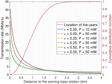
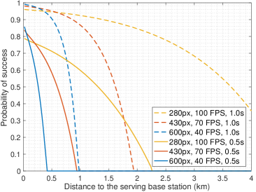
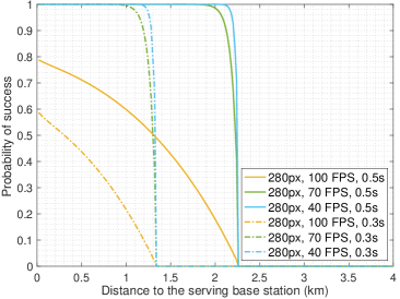
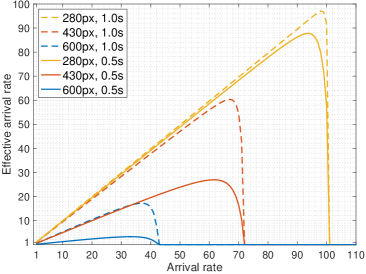
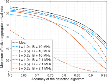
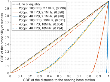
Figure 1: (a)-(c) Conditional transmission rate and probability of successful computation as a function of the distance between any randomly selected user and its serving base station. (d) Effective aggregate arrival rate as a function of the arrival rate. (e) Maximum effective aggregate arrival rate as a function of the accuracy of the detection algorithm. (f) Lorenz curve with Lorenz curve gap given in the legend. Figures (a)-(c) evaluate the relationship between the different parameters of the video analytics, of the uplink transmission, and of the edge server. Figures (d) and (e) analyze the effect of the system parameters on the effective arrival rate and on the accuracy of the detection algorithm. Finally, Figure (f) measures the disparity of the probability that an image is successfully processed, depending on the location of the users within the coverage area of their serving base station.

VI Discussion

Motivated by the recent advances in edge computing and artificial intelligence, we proposed a mathematical framework for modelling multi-cell, edge-intelligent systems supporting video analytics. We expressed the probability of successful computation and the effective arrival rate as a function of the accuracy of the video analytics, as well as the network and computing parameters. Our work provides the first steps towards designing efficient resource-allocation strategies and traffic-control protocols. We showed, for example, that different actions are necessary to improve the effective arrival rate, depending on whether the system is operating in bandwidth or computationally limited regimes. We also showed that the system can be highly unfair, and thus centralized solutions may be necessary to protect the weaker users. Further work should consider the modelling of more flexible bandwidth allocation and scheduling solutions, as well as protocol design.

References

- [1] J. Chen and X. Ran, “Deep learning with edge computing: A review.” Proc. IEEE, vol. 107, no. 8, pp. 1655–1674, 2019.
- [2] Z. Zhou, X. Chen, E. Li, L. Zeng, K. Luo, and J. Zhang, “Edge intelligence: Paving the last mile of artificial intelligence with edge computing,” Proceedings of the IEEE, vol. 107, no. 8, pp. 1738–1762, 2019.
- [3] F. Saeik, M. Avgeris, D. Spatharakis, N. Santi, D. Dechouniotis, J. Violos, A. Leivadeas, N. Athanasopoulos, N. Mitton, and S. Papavassiliou, “Task offloading in edge and cloud computing: A survey on mathematical, artificial intelligence and control theory solutions,” Computer Networks, vol. 195, p. 108177, 2021.
- [4] Q. Liu and T. Han, “Dare: Dynamic adaptive mobile augmented reality with edge computing,” in 2018 IEEE 26th International Conference on Network Protocols (ICNP). IEEE, 2018, pp. 1–11.
- [5] X. Ran, H. Chen, X. Zhu, Z. Liu, and J. Chen, “Deepdecision: A mobile deep learning framework for edge video analytics,” in IEEE INFOCOM 2018-IEEE Conference on Computer Communications. IEEE, 2018, pp. 1421–1429.
- [6] A. Galanopoulos, V. Valls, G. Iosifidis, and D. J. Leith, “Measurement-driven analysis of an edge-assisted object recognition system,” in ICC 2020-2020 IEEE International Conference on Communications (ICC). IEEE, 2020, pp. 1–7.
- [7] C. Wang, S. Zhang, Y. Chen, Z. Qian, J. Wu, and M. Xiao, “Joint configuration adaptation and bandwidth allocation for edge-based real-time video analytics,” in IEEE INFOCOM 2020-IEEE Conference on Computer Communications. IEEE, 2020, pp. 257–266.
- [8] S. Ko, K. Han, and K. Huang, “Wireless networks for mobile edge computing: Spatial modeling and latency analysis,” IEEE Transactions on Wireless Communications, vol. 17, no. 8, pp. 5225–5240, 2018.
- [9] S. Wang, W. Guo, and M. D. McDonnell, “Distance distributions for real cellular networks,” in 2014 IEEE Conference on Computer Communications Workshops (INFOCOM WKSHPS). IEEE, 2014, pp. 181–182.
- [10] S. N. Chiu, D. Stoyan, W. S. Kendall, and J. Mecke, Stochastic geometry and its applications. John Wiley & Sons, 2013.
- [11] T. D. Novlan, H. S. Dhillon, and J. G. Andrews, “Analytical modeling of uplink cellular networks,” IEEE Transactions on Wireless Communications, vol. 12, no. 6, pp. 2669–2679, 2013.
- [12] K. Sriram and W. Whitt, “Characterizing superposition arrival processes in packet multiplexers for voice and data,” IEEE journal on selected areas in communications, vol. 4, no. 6, pp. 833–846, 1986.
- [13] J. Redmon and G. Jocher, YOLOv5, 2021. [Online]. Available: https://github.com/ultralytics/yolov5
- [14] Q. Liu, S. Huang, J. Opadere, and T. Han, “An edge network orchestrator for mobile augmented reality,” in IEEE INFOCOM 2018-IEEE Conference on Computer Communications. IEEE, 2018, pp. 756–764.
- [15] A. Bochkovskiy, C.-Y. Wang, and H.-Y. M. Liao, “Yolov4: Optimal speed and accuracy of object detection,” arXiv preprint arXiv:2004.10934, 2020.
- [16] J. G. Andrews, F. Baccelli, and R. K. Ganti, “A tractable approach to coverage and rate in cellular networks,” IEEE Transactions on communications, vol. 59, no. 11, pp. 3122–3134, 2011.
- [17] R. P. Torres and J. R. Pérez, “A lower bound for the coherence block length in mobile radio channels,” Electronics, vol. 10, no. 4, p. 398, 2021.
- [18] V. B. Iversen, “Teletraffic engineering and network planning,” Technical University of Denmark, p. 270, 2010.
- [19] V. B. Iversen and L. Staalhagen, “Waiting time distribution in M/D/1 queueing systems,” Electronics Letters, vol. 35, no. 25, pp. 2184–2185, 1999.
- [20] A. Ghosh, J. Zhang, J. G. Andrews, and R. Muhamed, Fundamentals of LTE. Pearson Education, 2010.