Singularities of Gaussian Random Maps into the Plane

Abstract

We compute the expected value of various quantities related to the biparametric singularities of a pair of smooth centered Gaussian random fields on an $n$-dimensional compact manifold, such as the lengths of the critical curves and contours of a fixed index and the number of cusps. We obtain certain expressions under no particular assumptions other than smoothness of the two fields, but more explicit formulae are derived under varying levels of additional constraints such as the two random fields being i.i.d, stationary, isotropic etc.

1 Introduction

Let $N$ be an $n$-dimensional compact Riemannian manifold ($n\geq 2$). Given a smooth function

$$N\ni p\rightarrow h(p)=(f(p),g(p))\in\mathbb{R}^{2},$$

a point $p\in N$ is called a critical point if the derivative $Dh(p):T_{x}N\rightarrow\mathbb{R}^{2}$ at $p$ is not surjective and the set of all critical points is called the critical curve of $h$. The critical point is an example of a singularity of the smooth function $h$, and the objective of this paper is to study the expected value of various quantities of interest associated with such singularities when the components of $h$ are Gaussian random fields (GRFs). The expected number of critical points of a single GRF has been the subject of many papers e.g. [CS18, AAC13, AA13, ATW10, BBKS86, LH60], having applications in a wide variety of domains. The singularities of a pair of functions, being a two dimensional analogue of such one dimensional singularities, naturally warrant study. However, our main motivation to study these quantities come from biparametric persistent homology of smooth functions.

Persistent homology (PH) is a topological data analysis technique used to extract robust topological features from data. The key idea in single parameter PH is that if $X$ is a topological space and $f:X\rightarrow\mathbb{R}$ is a nice enough function on $X$, one can encode the change in homologies of the sublevel sets $\{f\leq a\}$ as the single parameter $a$ varies along the real line in the form of a simple planar diagram called the persistence diagram of $f$. If $X$ is a smooth manifold and $f$ is a Morse function, it is well known from Morse theory that the critical points of $f$ are precisely where the homology of its sublevel sets change, and hence the behavior of critical points of $f$ determine that of the persistence diagram of $f$. In biparametric persistence, one has a pair of functions $h=(f,g):X\rightarrow\mathbb{R}^{2}$ and one tries to track the change in homologies of the sublevel sets $\{f\leq a,g\leq b\}$ as the two parameters $(a,b)$ vary in the plane. When $X$ is a smooth manifold and the function $h$ is smooth, biparametric persistence can be understood from the perspective of Whitney theory, analogous to the Morse theoretic perspective of single parameter PH, and there is a growing amount of literature regarding this [CEF19, BK21, BC21, APKB21].

We give a brief description of this Whitney theoretic perspective on biparametric persistence here, the details of which can be found in [APKB21]. For a generic function $h$, the critical curve is a 1-dimensional embedded submanifold of $N$, or a disjoint finite union of smooth circles. The image of the critical curve under the map $h$ is called the visible contour. The visible contour will also be a finite union of closed curves in $\mathbb{R}^{2}$, although these curves may intersect each other and will be smooth only outside a finite number of points called cusps. The preimage of a cusp point can be characterized as a second order singularity of $h$, that is, a point of $N$ where the derivatives of $h$ upto order two satisfy certain conditions. In comparison, critical points are first order singularities of $h$ since their description only involves conditions on derivatives of $h$ upto order one. Figure 1(b) shows an example of a visible contour where the critical curve consists of a single circle. The visible contour is thus a single closed loop in $\mathbb{R}^{2}$, which has one point of self intersection and two cusp points where it loses smoothness.

At the image of the critical points of the component functions $f$ and $g$, the tangents to the visible contour are vertical and horizontal respectively. These points thus split the visible contour into segments with positive or negative slopes. The segments with negative slope are called Pareto segments of the visible contour. The curves indicated in black in Figure 1(c) are the Pareto segments of the visible contour shown in Figure 1(b). At the image of critical points of $f$ and $g$, we attach vertical and horizontal rays extending upward and rightward respectively, and call them the extension rays. The extension rays are the curves marked in blue in Figure 1(c).

The union of the Pareto segments of the visible contour and the extension rays is called the Pareto grid of $h$. The grid formed by the black and blue curves in Figure 1(c) form the Pareto grid of the visible contour in Figure 1(b). The Pareto grid has certain additional points of non-smoothness where a Pareto segment attaches to an extension ray in a non-smooth manner and these corner points are called pseudocusps. One can see that there are four non-smooth points on the Pareto grid in Figure 1(c) indicated in red, and two of these are cusps of the visible contour, while the other two are pseudocusps. The cusps and pseudocusps split the Pareto grid into multiple smooth pieces. These smooth pieces of the Pareto grid are the biparametric analogues of critical values in single parameter persistent homology. Homology generators are born or killed as the parameter value $(a,b)\in\mathbb{R}^{2}$ crosses these smooth pieces. One can define an index for each of these pieces determining the dimension of the cell attached at a crossing as well.

(a) Chicago Millenium Park

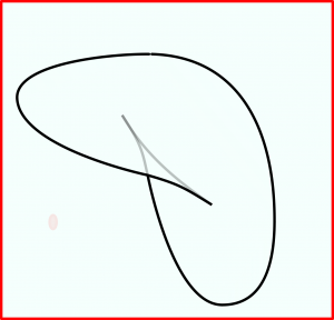
(b) Visible contour

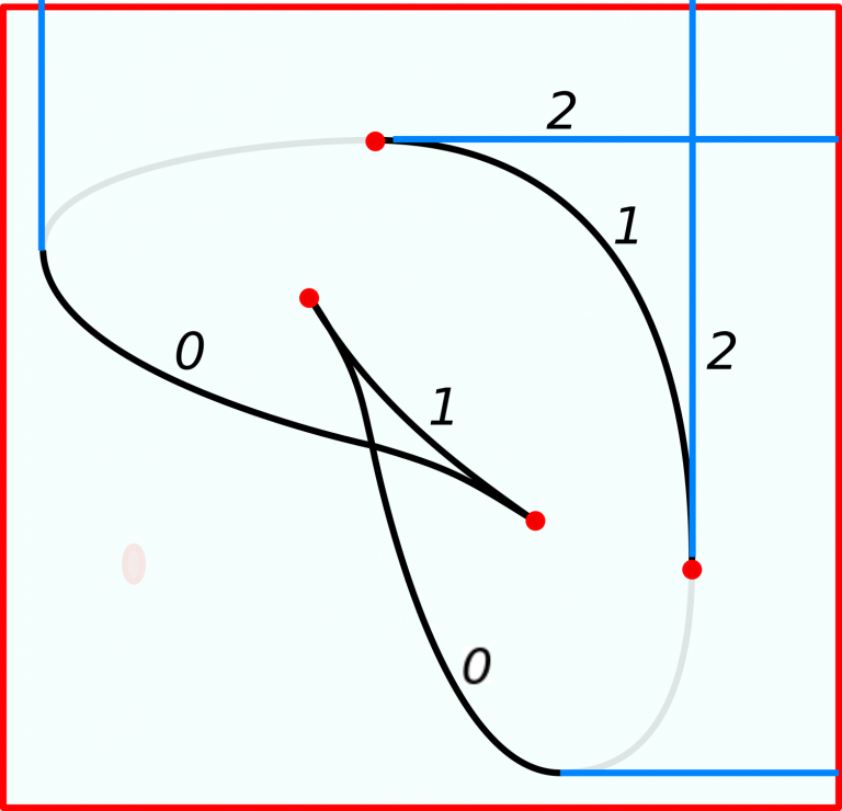
(c) Pareto grid

Figure 1: Figure (a) shows a bean sculpture, the surface of which is a two dimensional sphere. If $h$ is the projection of the surface onto a plane behind the bean the corresponding visible contour is shown in Figure (b). The Pareto grid, along with cusps, pseudocusps and indices of various segments of the grid are shown in Figure (c).

The objective of this article is to study some statistical properties of these biparametric singularities of a GRF $h$. Given the Whitney theoretic description of biparametric persistence, understanding the properties of these singularities give us an idea about the complexity of the biparametric persistence of GRFs into the plane. We will mainly focus on computing the expected lengths of the critical curve and visible contour of each index. Unlike critical points, the cusp points are second order singularities which means their characterization involves derivatives upto order two. If we were to use the Kac-Rice formula [AT07, Theorem 12.1.1] to compute the expected number of cusps, the computations will involve derivatives of $h$ upto order three making them really cumbersome. Hence, these computations are left to a later paper. However, the expected number of pseudocusps can be computed using standard techniques as they are critical points of single variable GRFs and these computations are done in the article.

We derive expressions for these expectations for general pairs of GRFs, assuming only that they are smooth and centered (mean zero) and some additional mild technical assumptions. The expressions yield neater formulae as more assumptions such as the pair of GRFs being identical and independent, stationary or isotropic are imposed. However, all the general expressions we find here are written as expectations of functions of certain Gaussian random vectors and Gaussian random matrices. The additional assumptions on the GRFs make the distributions of these random vectors and matrices nicer, such as being independent, rotationally invariant etc. yielding better closed form solutions.

The paper is structured as follows. The remaining part of section 1 introduces the notations and assumptions used in the article. In section 2, we derive expressions for the expected length of the critical curve, visible contour and Pareto segments, each of a fixed index. This section doesn’t assume much about the GRF $h$ beyond begin smooth and centered. In section 3, we simplify the expressions obtained in the previous section under the additional assumption that the component functions $f$ and $g$ are independent and identically distributed GRFs. We also show concrete examples of these computations in two settings, random bandlimited functions into the plane and random planar projections of the standard embedded torus in $\mathbb{R}^{3}$. In section 4, we obtain neater formulae under the assumptions that the manifold $N$ is the $n$-sphere $\S^{n}$ and the component GRFs $f$ and $g$ are isotropic and stationary. Finally, in section 5, we derive the expected number of pseudocusps of a fixed index.

1.1 Notation

We denote by $N$ an $n$-dimensional compact orientable Riemannian manifold endowed with a Riemannian metric $G$. The corresponding volume form on $N$ will be denoted by $d_{N}V$. We will deal with certain one dimensional compact submanifolds on $N$, and the volume form endowed by the induced Riemannian metric on them will be denoted by $d_{N}l$. $S^{1}$ will denote the unit circle endowed with the standard Riemannian metric. We will also need to look at certain one dimensional compact submanifolds on the product space $S^{1}\times N$ endowed with the product Riemannian metric and the volume form endowed by the induced Riemannian metric on them will be denoted by $d_{S^{1}\times N}l$.

Some of the computations in the article will be done in coordinate charts on $N$ and if $v\in\mathbb{R}^{n}$ is the coordinate representation of a tangent vector on $N$, $\|v\|_{G}$ will denote its norm in the Riemannian metric while $\|v\|$ will denote its usual Euclidean norm.

$J^{r}(N,\mathbb{R}^{2})$ is the $r$-jet space of $N$ to $\mathbb{R}^{2}$ and $J_{p}^{r}(N,\mathbb{R}^{2})$ is the $r$-jet space at $p\in N$, which are both Euclidean spaces since the codomain $\mathbb{R}^{2}$ is Euclidean. We denote by $S_{k}$ the corank $k$ submanifold of $J^{1}(N,\mathbb{R}^{2})$ consisting of those jets with rank $2-k$. Given a smooth function $h:N\rightarrow\mathbb{R}^{2}$, we denote by $j^{r}h:N\rightarrow J^{r}(N,\mathbb{R}^{2})$ its $r$-jet function (see [GG12] for details).

$$N\times\Omega\ni(p,\omega)\rightarrow h(p,\omega)=(f(p,\omega),g(p,\omega))\in\mathbb{R}^{2}$$

will denote a Gaussian random field (GRF) on $N$. To make notations less cumbersome, we will avoid including $\omega$ and refer to $h(p)$ freely as a GRF. The support of $h$ is defined as

$$\text{supp}\left(h\right)=\{\bar{h}\in C^{\infty}(N,\mathbb{R}^{2})\text{ such that }\mathbb{P}\left(h\in U\right)>0\text{ for all neighborhoods $U$ of }\bar{h}\}.$$

(see [S⁺20] for more details). If $h$ is smooth almost surely, its derivatives are also GRFs and so is $j^{r}h$. If $W$ is a submanifold of $J^{r}(N,\mathbb{R}^{2})$, then $j^{r}h\pitchfork W$ will denote that the function $j^{r}h$ intersects $W$ transversally.

1.2 Assumptions

There are three standing assumptions throughout the article.

Assumption 1.1.

The GRF $h$ is centered, that is, $\mathsf{E}\!\left[\vphantom{\big{|}}h(p)\vphantom{\big{|}}\right]=0$ for all $p\in N$.

Our techniques and proofs work identically in the non-centered case as well, but the final formulae obtained are not very clean and exact computation is not possible when the mean is not zero.

Assumption 1.2.

The GRF $h$ is smooth on $N$ almost surely.

This is not too strict an assumption, as there are conditions on the GRF that ensures this happens, such as [AT07, Theorem 11.3.4].

Assumption 1.3.

The support of the 2-jet ${\text{supp}}\left(j^{2}h(p)\right)=J^{2}_{p}(N,\mathbb{R}^{2})$ for all $p\in N$, that is, the jointly Gaussian random vector

$$\left(f(p),g(p),\nabla f(p),\nabla g(p),\nabla^{2}f(p),\nabla^{2}g(p)\right)$$

is non degenerate.

Smoothness of $h$ isn’t the only regularity condition we need for our computations; we will require the $r$-jet of $h$ satisfy certain non-degeneracy conditions. We will see that the above assumption on a GRF, along with the following lemma, will be required to ensure this happens almost surely.

Lemma 1.4 ([S⁺20], Theorem 23).

Let $h:N\rightarrow\mathbb{R}^{2}$ be a smooth GRF and $r\in\mathbb{N}$. Assume that for every $p\in N$ we have ${\text{supp}}\left(j^{r}h(p)\right)=J_{p}^{r}(N,\mathbb{R}^{2})$. Then for any submanifold $W\subset J^{r}(N,\mathbb{R}^{2})$, we have $\mathbb{P}\left(j^{r}h\pitchfork W\right)=1.$

2 Length computations on general centered GRFs

2.1 Expected length of critical curves

In this section, we derive expressions for the average length of the critical curve of $h$. Recall that a point $p\in N$ is called a critical point of $h$ if the derivative $Dh(p):T_{x}N\rightarrow\mathbb{R}^{2}$ at $p$ is not surjective. This is equivalent to saying that the gradient vectors $\nabla f(p),\nabla g(p)$ are not linearly independent vectors lying in the tangent space $T_{p}N$. The set of critical points of $h$ is called the critical set of $h$. For a generic function $h$ the critical set will be a 1-dimensional embedded submanifold of $N$, or a collection of disjoint embedded circles in $N$, justifying the term critical curve.

Lemma 2.1.

If $h$ satisfies assumptions 1.1-1.3 then the critical curve of $h$ is a one dimensional compact submanifold of $N$ on which the rank of $Dh$ is 1 almost surely.

Proof.

The critical curve $\Sigma_{c}=\left(j^{1}h\right)^{-1}\left(S_{1}\cup S_{2}\right).$ This means that the critical curve is closed, as $S_{1}\cup S_{2}$ is a closed subset of $J^{1}(N,\mathbb{R}^{2})$. As a consequence of Lemma 1.4, Assumption 1.3 guarantees that

$$\mathbb{P}\left(j^{1}h\pitchfork W\right)=1$$

for any submanifold $W\subset J^{1}(N,\mathbb{R}^{2})$. This implies $j^{1}h\pitchfork S_{r}$ for $r=1,2$ almost surely. Since $\operatorname{codim}(S_{2})=2n>\dim(N)$, $\left(j^{1}h\right)^{-1}S_{2}$ is empty. Therefore, the critical curve $\Sigma_{c}=\left(j^{1}h\right)^{-1}\left(S_{1}\right).$ Since $j^{1}h$ intersects $S_{1}$ transversally, $\Sigma_{c}$ is a submanifold of $N$. In addition,

$$\operatorname{codim}\left(S_{1}\right)=n-1\implies\operatorname{codim}(\Sigma_{c})=n-1\implies\dim(\Sigma_{c})=1.$$

∎

We are now in a position where the length of the critical curve makes sense almost surely, and will derive expressions for the average length in local coordinates first and then show that the expressions are coordinate invariant. Let $x=(x_{1},x_{2},...,x_{n})$ be local coordinates on a coordinate neighborhood $U$ of $N$, that is,

$$\mathbb{R}^{n}\ni(x_{1},...,x_{n})=x\longrightarrow\phi(x)=p\in U$$

is a diffeomorphism. Let $K\subset U$ be the coordinate image of a compact set in $\mathbb{R}^{n}$. To avoid notational clutter, we will refer to the local representation of $h$ (and $f,g$) as $h$ itself. We can characterize the critical points in these coordinates as the projection onto $N$ of the zeros of the $\mathbb{R}^{n}$ valued function

$$U\times S^{1}\ni(x,\theta)\longrightarrow V(x,\theta)=\cos(\theta)\nabla f(x)+\sin(\theta)\nabla g(x)\in\mathbb{R}^{n}.$$ (1)

We also define the infinitesimal length vector $LV(x,\theta)$ as

$$LV(x,\theta)=\operatorname{adj}\left(\nabla_{x}V(x,\theta)\right)\nabla_{\theta}V(x,\theta).$$

The following local result will be our first step.

Proposition 2.2.

If the GRF $h$ satisfies assumptions 1.1-1.3 and $K$ is a compact set contained in a coordinate chart $U$, then the expected value of the length of the critical curve in $K$ is

$$\mathsf{E}\!\left[\vphantom{\big{|}}\operatorname{len}(\Sigma_{c}\cap K)\vphantom{\big{|}}\right]=\int_{K}\int_{[0,\pi]}\frac{\mathsf{E}\!\left[\vphantom{\big{|}}\|LV(x,\theta)\|_{G}\bigg{|}V(x,\theta)=0\vphantom{\big{|}}\right]}{\sqrt{(2\pi)^{n}\det(G(x)\mathsf{Var}\!\left[\vphantom{\big{|}}V(x,\theta)\vphantom{\big{|}}\right])}}d_{N}Vd\theta.$$ (2)

We will prove 2.2 after defining a few more objects and establishing a sequence of lemmas. Define the $S^{1}$ indexed family of real valued GRFs $h_{\theta}$ as

$$N\ni p\longrightarrow h_{\theta}(p):=\cos(\theta)f(p)+\sin(\theta)g(p)\in\mathbb{R}.$$

Lemma 2.3.

If $h$ is a GRF satisfying assumptions 1.1-1.3, then $h_{\theta}$ is a Morse function outside finitely many pairs $(p,\theta)$, almost surely. The function $N\times S^{1}\ni(p,\theta)\longrightarrow h_{R}(\theta,p):=h_{\theta}(p)\in\mathbb{R}$ is also a Morse function almost surely.

Proof.

Let $W$ be the submanifold of $J^{2}(N\times S^{1},\mathbb{R})$ defined as

$$W=\big{\{}j^{2}f(p,\theta)\big{|}\ f:N\times S^{1}\longrightarrow\mathbb{R},\ D_{1}f(p,\theta)=0,\ \operatorname{rk}(D^{2}_{1,1}f(p,\theta))=n-1\big{\}}$$

which satisfies $\operatorname{codim}(W)=n+1$. Assumption 1.3 and Lemma 1.4 tells us that $j^{2}h_{R}\pitchfork W$ almost surely. Therefore, $Z=(j^{2}h_{R})^{-1}(W)$ is a codimension $n+1$ submanifold of $N\times S^{1}$, i.e. a finite set of points. $h_{\theta}$ is not Morse at $(p,\theta)$ iff $(p,\theta)\in Z$, which proves the first part of the lemma.

We use the fact that $h_{R}$ is a Morse function only if $j^{1}h_{R}\pitchfork S_{1}\subset J^{1}(N\times S^{1},\mathbb{R})$, where $S_{1}$ denotes the corank-1 submanifold of $J^{1}(N\times S^{1},\mathbb{R})$ [GG12, Proposition 6.4]. Assumption 1.3 guarantees that the GRF $h_{R}:N\times S^{1}\longrightarrow\mathbb{R}$ satisfies ${\text{supp}}\left(j^{1}h_{R}(p,\theta)\right)=J_{\left(p,\theta\right)}^{1}(N\times S^{1},\mathbb{R})$. Lemma 1.4 then says that $j^{1}h_{R}\pitchfork S_{1}$ almost surely, which means $h_{R}$ is a Morse function almost surely.

∎

Note that $V(x,\theta)$ is just the derivative of $h_{\theta}$ in local coordinates. The fact that $h_{\theta}$ is a Morse function ensures that

$$\nabla_{x}V(x,\theta)=\cos(\theta)\nabla^{2}f(x)+\sin(\theta)\nabla^{2}g(x).$$ (3)

is non-degenerate at points where $V(x,\theta)=0$, excluding finitely many points on the critical curve. Since the length of the critical curve is not affected by removing finitely many points, we can ignore these points and proceed. This means that $V(x,\theta)$ is a submersion on $V^{-1}(0)$, which further implies that $V^{-1}(0)$ is a one dimensional submanifold of $U\times S^{1}$. If $\pi:N\times S^{1}\rightarrow N$ denotes projection to the first factor, then $\pi(V^{-1}(0))=\Sigma_{c}\cap U$. We denote by $dl$ the volume form on $V^{-1}(0)$ corresponding to the metric induced on it by the Euclidean metric on $\mathbb{R}^{n}\times S^{1}$. Similarly, $d_{N}l$ denotes the volume form on $\Sigma_{c}$ corresponding to the metric induced by the Riemannian metric on $N$.

Lemma 2.4.

If $h$ is a GRF satisfying assumptions 1.1-1.3, then the following equation holds almost surely.

$$\operatorname{len}(\Sigma_{c}\cap K)=\frac{1}{2}\int_{V^{-1}(0)\cap(K\times S^{1})}\frac{\|LV(x,\theta)\|_{G}}{\sqrt{\det(\nabla_{x}V(x,\theta))^{2}+\|LV(x,\theta)\|^{2}}}dl.$$

Proof.

The fact that $\nabla_{x}V(x,\theta)$ is non-degenerate implies that $V^{-1}(0)$ can be locally parametrized by $\theta$, as per the implicit function theorem. We will denote this parametrization by $x(\theta)$. The derivative of this function is then

$$\frac{dx}{d\theta}=(\nabla_{x}V(x,\theta))^{-1}(\nabla_{\theta}V(x,\theta))=\frac{\operatorname{adj}\left(\nabla_{x}V(x,\theta)\right)\nabla_{\theta}V(x,\theta)}{\det\left(\nabla_{x}V(x,\theta)\right)}.$$

Since $\pi:V^{-1}(0)\rightarrow\Sigma_{c}\cap U$ is a double cover of the critical curve,

$$\int_{\Sigma_{c}\cap K}d_{N}l=\frac{1}{2}\int_{V^{-1}(0)\cap(K\times S^{1})}\pi^{*}d_{N}l.$$

We know that $(\frac{dx}{d\theta},1)$ lies tangent to $V^{-1}(0)$. Then,

$$\pi^{*}d_{N}l\left(\frac{dx}{d\theta},1\right)=d_{N}l\frac{dx}{d\theta}=\|\frac{dx}{d\theta}\|_{G},\quad dl\left(\frac{dx}{d\theta},1\right)=\sqrt{1+\|\frac{dx}{d\theta}\|^{2}},$$

$$\implies\pi^{*}d_{N}l=\frac{\|\frac{dx}{d\theta}\|_{G}}{\sqrt{1+\|\frac{dx}{d\theta}\|^{2}}}dl=\frac{\|\operatorname{adj}\left(\nabla_{x}V(x,\theta)\right)\nabla_{\theta}V(x,\theta)\|_{G}}{\sqrt{\det(\nabla_{x}V(x,\theta))^{2}+\|\operatorname{adj}\left(\nabla_{x}V(x,\theta)\right)\nabla_{\theta}V(x,\theta)\|^{2}}}dl,$$

which proves the result. ∎

Proof of proposition 2.2.

In lemma 2.4, we expressed the length of the critical curve as a weighted integral over the level set of the real valued GRF $V(x,\theta)$ on $U\times S^{1}$. To find the expectation of this weighted integral, we apply the generalized Rice formula ([AW09, Theorem 6.10]). Assumption 1.3 along with lemma 2.1 ensure that the conditions required ((i)-(iv) in [AW09, Theorem 6.8]) to justify this are satisfied. If we denote the total derivative of $V$ by

$$\nabla V(x,\theta)=\bigg{[}\nabla_{x}V(x,\theta)\quad\nabla_{\theta}V(x,\theta)\bigg{]},$$

then

$$\mathsf{E}\!\left[\vphantom{\big{|}}\operatorname{len}(\Sigma_{c}\cap K)\vphantom{\big{|}}\right]=\frac{1}{2}\int_{K}\int_{S^{1}}\mathsf{E}\!\left[\vphantom{\big{|}}\det\left(\nabla V.\nabla V^{\top}\right)^{\frac{1}{2}}\frac{\|\operatorname{adj}(\nabla_{x}V)\nabla_{\theta}V\|_{G}}{\sqrt{\det(\nabla_{x}V)^{2}+\|\operatorname{adj}(\nabla_{x}V)\nabla_{\theta}V\|^{2}}}\bigg{|}V=0\vphantom{\big{|}}\right]p_{V}(0)dxd\theta,$$

where we have dropped the obvious $(x,\theta)$ dependence to avoid clutter. Observe that

$$\det\left(\nabla V.\nabla V^{\top}\right) =\det\left(\nabla_{x}V.\nabla_{x}V^{\top}+\nabla_{\theta}V.\nabla_{\theta}V^{\top}\right)$$

$$=\det(\nabla_{x}V)^{2}\det\left(I+\left(\nabla_{x}V^{-1}\nabla_{\theta}V\right)\left(\nabla_{x}V^{-1}\nabla_{\theta}V\right)^{\top}\right)$$

$$=\det(\nabla_{x}V)^{2}\left(1+\|\nabla_{x}V^{-1}\nabla_{\theta}V\|^{2}\right)=\det(\nabla_{x}V)^{2}+\|\operatorname{adj}(\nabla_{x}V)\nabla_{\theta}V\|^{2}.$$

In addition, $p_{V(x,\theta)}(0)$ is the density of $V(x,\theta)$ evaluated at $0$. Since $V(x,\theta)$ is an $n$-dimensional mean zero Gaussian random vector,

$$p_{V(x,\theta)}(0)=(2\pi)^{\frac{-n}{2}}(\det(\mathsf{Var}\!\left[\vphantom{\big{|}}V(x,\theta)\vphantom{\big{|}}\right])^{\frac{-1}{2}}.$$

In total, we get

$$\mathsf{E}\!\left[\vphantom{\big{|}}\operatorname{len}(\Sigma_{c}\cap K)\vphantom{\big{|}}\right]=\frac{1}{2(2\pi)^{\frac{n}{2}}}\int_{K}\int_{S^{1}}\frac{\mathsf{E}\!\left[\vphantom{\big{|}}\|\operatorname{adj}(\nabla_{x}V(x,\theta))\nabla_{\theta}V(x,\theta)\|_{G}\bigg{|}V(x,\theta)=0\vphantom{\big{|}}\right]}{\sqrt{\det(\mathsf{Var}\!\left[\vphantom{\big{|}}V(x,\theta)\vphantom{\big{|}}\right])}}dxd\theta.$$

The Riemannian volume form on $N$ is related to the Euclidean volume form $dx$ as

$$d_{N}V=\sqrt{\det(G(x))}dx.$$

In addition, observe that $\nabla_{x}V(x,\theta+\pi)=-\nabla_{x}V(x,\theta),\nabla_{\theta}V(x,\theta+\pi)=-\nabla_{\theta}V(x,\theta)$. Therefore, we can say that

$$\mathsf{E}\!\left[\vphantom{\big{|}}\operatorname{len}(\Sigma_{c}\cap K)\vphantom{\big{|}}\right]=\int_{K}\int_{[0,\pi]}\frac{\mathsf{E}\!\left[\vphantom{\big{|}}\|\operatorname{adj}(\nabla_{x}V(x,\theta))\nabla_{\theta}V(x,\theta)\|_{G}\bigg{|}V(x,\theta)=0\vphantom{\big{|}}\right]}{\sqrt{(2\pi)^{n}\det(G(x)\mathsf{Var}\!\left[\vphantom{\big{|}}V(x,\theta)\vphantom{\big{|}}\right])}}d_{N}Vd\theta.$$

∎

We now show that the integrand in (2) is coordinate invariant. Let

$$\mathbb{R}^{n}\ni(y_{1},...,y_{n})=y\longrightarrow\psi(y)\in U$$

be another coordinate chart on $U$. Let $J$ be the Jacobin of the coordinate change map from $(y_{1},...,y_{n})\rightarrow(x_{1},...,x_{n})$. Then

$$V(x,\theta)=J^{\top}V(y,\theta),\quad\nabla_{\theta}V(x,\theta)=J^{\top}V(y,\theta),\quad\nabla_{x}V(x,\theta)=J^{\top}\nabla_{y}V(y,\theta)J.$$

The Riemannian metric tensor transforms as $G(x)=J^{\top}G(y)J$. This means

$$\operatorname{adj}(\nabla_{x}V(x,\theta))\nabla_{\theta}V(x,\theta) =\det(J)^{2}J^{-1}\operatorname{adj}(\nabla_{y}V(y,\theta)J^{-\top}J^{\top}\nabla_{\theta}V(y,\theta)$$

$$=\det(J)^{2}J^{-1}\nabla_{y}V(y,\theta)\nabla_{\theta}V(y,\theta),$$

$$\sqrt{\det(G(x)\mathsf{Var}\!\left[\vphantom{\big{|}}V(x,\theta)\vphantom{\big{|}}\right])} =\det(J)^{2}\sqrt{\det(G(y)\mathsf{Var}\!\left[\vphantom{\big{|}}V(y,\theta)\vphantom{\big{|}}\right]}.$$

We can write

$$\|\operatorname{adj}(\nabla_{x}V(x,\theta)) \nabla_{\theta}V(x,\theta)\|_{G}=\nabla_{\theta}V(x,\theta)^{\top}\operatorname{adj}(\nabla_{x}V(x,\theta))^{\top}G(x)\operatorname{adj}(\nabla_{x}V(x,\theta))\nabla_{\theta}V(x,\theta)$$

$$=(\det(J))^{2}\nabla_{\theta}V(y,\theta)^{\top}\operatorname{adj}(\nabla_{y}V(y,\theta))^{\top}J^{-\top}G(x)J^{-1}\operatorname{adj}(\nabla_{y}V(y,\theta))\nabla_{\theta}V(y,\theta)$$

$$=(\det(J))^{2}\nabla_{\theta}V(y,\theta)^{\top}\operatorname{adj}(\nabla_{y}V(y,\theta))^{\top}G(y)\operatorname{adj}(\nabla_{y}V(y,\theta))\nabla_{\theta}V(y,\theta)$$

$$=(\det(J))^{2}\|\operatorname{adj}(\nabla_{y}V(y,\theta))\nabla_{\theta}V(y,\theta)\|_{G}$$

which immediately gives coordinate invariance of the integrand. We can now give each term in the integrand the following coordinate invariant characterization:

$$V(x,\theta) \longrightarrow\nabla h_{\theta}(p),\nabla_{x}V(x,\theta)\longrightarrow\nabla^{2}h_{\theta}(p),\nabla_{\theta}V(x,\theta)\longrightarrow\nabla h_{\theta+\frac{\pi}{2}}(p).$$

If we define

$$\left[\mathsf{Var}\!\left[\vphantom{\big{|}}\nabla h_{\theta}(p)\vphantom{\big{|}}\right]\right]_{i,j}:=\mathsf{E}\!\left[\vphantom{\big{|}}(\nabla h_{\theta}(p).v_{i})(\nabla h_{\theta}(p).v_{j})\vphantom{\big{|}}\right]$$

where $\{v_{i}\}_{i=1}^{n}$ is an orthonormal basis of $T_{p}N$, then

$$\det(\mathsf{Var}\!\left[\vphantom{\big{|}}\nabla h_{\theta}(p)\vphantom{\big{|}}\right])=\det(G(x)\mathsf{Var}\!\left[\vphantom{\big{|}}V(x,\theta)\vphantom{\big{|}}\right]).$$

We can now extend proposition 2.2 globally to get the main result of this section.

Theorem 2.5.

If the GRF $h$ satisfies assumptions 1.1-1.3, then the expected value of the length of its critical curve is

$$\mathsf{E}\!\left[\vphantom{\big{|}}\operatorname{len}(\Sigma_{c})\vphantom{\big{|}}\right]=\int_{N}\int_{[0,\pi]}\frac{\mathsf{E}\!\left[\vphantom{\big{|}}\|\operatorname{adj}\left(\nabla^{2}h_{\theta}(p)\right)\nabla h_{\theta+\frac{\pi}{2}}(p)\|_{G}\bigg{|}\nabla h_{\theta}(p)=0\vphantom{\big{|}}\right]}{\sqrt{(2\pi)^{n}\det\left(\mathsf{Var}\!\left[\vphantom{\big{|}}\nabla h_{\theta}(p)\vphantom{\big{|}}\right]\right)}}dVd\theta.$$ (4)

Proof.

Cover the manifold $N$ by a finite number of compact coordinate disks $K_{i},\ i=1,...,k$. We already know

$$\mathsf{E}\!\left[\vphantom{\big{|}}\operatorname{len}(\Sigma_{c})\cap K_{i}\vphantom{\big{|}}\right]=\int_{K_{i}}\int_{[0,\pi]}\frac{\mathsf{E}\!\left[\vphantom{\big{|}}\|\operatorname{adj}\left(\nabla^{2}h_{\theta}(p)\right)\nabla h_{\theta+\frac{\pi}{2}}(p)\|_{G}\bigg{|}\nabla h_{\theta}(p)=0\vphantom{\big{|}}\right]}{\sqrt{(2\pi)^{n}\det\left(\mathsf{Var}\!\left[\vphantom{\big{|}}\nabla h_{\theta}(p)\vphantom{\big{|}}\right]\right)}}dVd\theta.$$

By the inclusion exclusion principle,

$$\mathsf{E}\!\left[\vphantom{\big{|}}\operatorname{len}{\Sigma_{c}}\vphantom{\big{|}}\right]=\sum\limits_{l=1}^{k}\sum_{i_{1}<i_{2}<...<i_{l}}(-1)^{l+1}\mathsf{E}\!\left[\vphantom{\big{|}}\operatorname{len}{\Sigma_{c}\cap K_{i_{1}}\cap K_{i_{2}}...\cap K_{i_{l}}}\vphantom{\big{|}}\right].$$

But the integral of any function $f:N\rightarrow\mathbb{R}$ can be written as

$$\int_{N}fd_{N}V=\sum\limits_{l=1}^{k}\sum_{i_{1}<i_{2}<...<i_{l}}(-1)^{l+1}\int_{\cap_{j=1}^{l}K_{i_{j}}}fd_{N}V,$$

from which the result follows directly. ∎

Remark 2.6.

Notice that $(\nabla^{2}h_{\theta},\nabla h_{\theta+\frac{\pi}{2}},\nabla h_{\theta})$ are jointly Gaussian random vectors and so the conditional expectation in (4) is just the expectation of a function of a Gaussian random vector.

2.2 Expected length of the visible contour

A point $v\in\mathbb{R}^{2}$ is called a critical value of $h$ if the preimage $h^{-1}\{v\}$ contains a critical point, that is, $\gamma_{c}=h(\Sigma_{c})$. The subset of $\mathbb{R}^{2}$ consisting of all critical values is called the visible contour $\gamma_{c}$ of $h$. In this section, we will compute the average length of the visible contour of $h$ in this section.

The computation of the expected length of the visible contour follows the exact same procedure as the one we saw in the previous section. We have the following analogues of proposition 2.2, lemma 2.4.

Proposition 2.7.

If the GRF $h$ satisfies assumptions 1.1-1.3 and $K$ is a compact set contained in a coordinate chart $U$, then the expected value of the length of its critical curve in $K$ is

$$\mathsf{E}\!\left[\vphantom{\big{|}}\operatorname{len}(h(\Sigma_{c}\cap K))\vphantom{\big{|}}\right]=\int_{K}\int_{[0,\pi]}\frac{\mathsf{E}\!\left[\vphantom{\big{|}}\left|\nabla_{\theta}V(x,\theta)^{\top}LV(x,\theta)\right|\bigg{|}V(x,\theta)=0\vphantom{\big{|}}\right]}{\sqrt{(2\pi)^{n}\det(G(x)\mathsf{Var}\!\left[\vphantom{\big{|}}V(x,\theta)\vphantom{\big{|}}\right])}}d_{N}Vd\theta.$$ (5)

Lemma 2.8.

If $h$ is a GRF satisfying assumptions 1.1-1.3, then the following equation holds almost surely.

$$\operatorname{len}(\Sigma_{c}\cap K)=\frac{1}{2}\int_{V^{-1}(0)\cap(K\times S^{1})}\frac{\left|\nabla_{\theta}V(x,\theta)^{\top}LV(x,\theta)\right|}{\sqrt{\det(\nabla_{x}V(x,\theta))^{2}+\|LV(x,\theta)\|^{2}}}dl.$$

Proof.

Here we have the sequence of maps

$$V^{-1}(0)\overset{\pi}{\longrightarrow}\Sigma_{c}\cap U\overset{h}{\longrightarrow}\gamma_{c}.$$

If we denote by $d_{\mathbb{R}^{2}}l$ the volume form on $\gamma_{c}$ outside a finite set of cusps) induced from the Euclidean metric on $R^{2}$, we can say that

$$\int_{h(\Sigma_{c}\cap K)}d_{\mathbb{R}^{2}}l=\frac{1}{2}\int_{V^{-1}(0)\cap(K\times S^{1})}(h\circ\pi)^{*}d_{\mathbb{R}^{2}}l.$$

We know that $(\frac{dx}{d\theta},1)$ lies tangent to $V^{-1}(0)$. Then,

$$(h\circ\pi)^{*}d_{\mathbb{R}^{2}}l\left(\frac{dx}{d\theta},1\right)=d_{\mathbb{R}^{2}}l\left(Dh\frac{dx}{d\theta}\right)=\|Dh\frac{dx}{d\theta}\|,\quad dl\left(\frac{dx}{d\theta},1\right)=\sqrt{1+\|\frac{dx}{d\theta}\|^{2}}.$$

Since the Euclidean norm on $\mathbb{R}^{2}$ is invariant under rotation by an angle $\theta$, we can say

$$\|Dh\frac{dx}{d\theta}\|=\left\|\begin{bmatrix}\left(\cos(\theta)\nabla f(x)+\sin(\theta)\nabla g(x)\right)^{\top}\\ \left(-\sin(\theta)\nabla f(x)+\cos(\theta)\nabla g(x)\right)^{\top}\end{bmatrix}\frac{dx}{d\theta}\right\|.$$ (6)

However, since $\cos(\theta)\nabla f(x)+\sin(\theta)\nabla g(x)=0$, we can further rewrite this term as

$$\left|\left\langle-\sin(\theta)\nabla f(x)+\cos(\theta)\nabla g(x),\frac{dx}{d\theta}\right\rangle\right|=\left|\nabla_{\theta}V(x,\theta)^{\top}(\nabla_{x}V(x,\theta))^{-1}\nabla_{\theta}V(x,\theta)\right|.$$ (7)

Therefore,

$$(h\circ\pi)^{*}d_{\mathbb{R}^{2}}l=\frac{\|Dh\frac{dx}{d\theta}\|}{\sqrt{1+\|\frac{dx}{d\theta}\|^{2}}}=\frac{|\nabla_{\theta}V(x,\theta)^{\top}\operatorname{adj}(\nabla_{x}V(x,\theta)\nabla_{\theta}V(x,\theta)|}{\sqrt{\det(\nabla_{x}V(x,\theta))^{2}+\|\operatorname{adj}(\nabla_{x}V(x,\theta)\nabla_{\theta}V(x,\theta)\|^{2}}}dl.$$

from which the result follows through the exact same steps as in the proof of lemma 2.4. ∎

The rest of the computations and justifications in the proof of 2.7 also follow the exact same pattern as in the proof of 2.2, and won’t be repeated. The main result of this section also follows from 2.7 as

Theorem 2.9.

If the GRF $h$ satisfies assumptions 1.1-1.3, then the expected value of the length of its visible contour is

$$\mathsf{E}\!\left[\vphantom{\big{|}}\operatorname{len}(\gamma_{c})\vphantom{\big{|}}\right]=\int_{N}\int_{[0,\pi]}\frac{\mathsf{E}\!\left[\vphantom{\big{|}}\left|\nabla h_{\theta+\frac{\pi}{2}}^{\top}\operatorname{adj}\left(\nabla^{2}h_{\theta}(p)\right)\nabla h_{\theta+\frac{\pi}{2}}(p)\right|\bigg{|}\nabla h_{\theta}(p)=0\vphantom{\big{|}}\right]}{\sqrt{(2\pi)^{n}\det\left(\mathsf{Var}\!\left[\vphantom{\big{|}}\nabla h_{\theta}(p)\vphantom{\big{|}}\right]\right)}}dVd\theta.$$ (8)

Remark 2.10.

The length of the visible contour does not depend on the choice of metric on $N$. Indeed, the formula given in equation (8) is invariant under a change of metric, since $\frac{dV}{\sqrt{\det G}}$ does not depend on the choice of metric.

Remark 2.11.

The Pareto segments of the visible contour are the parts of the contour where its slope is negative. The segments of the contour play a special role in biparametric persistent homology and the length of only these parts can also be easily computed. The only observation needed to do this is that $h(x)$ lies on the Pareto segment only if $\theta$ lies in $[0,\frac{\pi}{2}]$. So one simply needs to replace the domain of evaluation of the inner $\theta$ integral in (8) with $[0,\frac{\pi}{2}]$.

2.3 Expected length of segments of fixed index

The index of a critical point (and the corresponding critical value) of a single function $f$ refers to the index of the Hessian of $f$ at the critical point. The significance of the index is that if $f(p)$ is a critical value of index $k$, then the sublevel set $\{f\leq f(p)+\epsilon\}$ is obtained by attaching a $k$-cell to $\{f\leq f(p)-\epsilon\}$ as long as $(f(p)-\epsilon,f(p)+\epsilon)$ contains no other critical values. In the single persistent homology setting, this translates to the fact that an index $k$ critical value can either lead to a birth in $k$-th homology or a death in $k+1$-th homology.

The Pareto segments of the visible contour plays a similar role in bi-biparametric persistence. If $p$ is a critical point of $h$ and the corresponding value $v=(f(p),g(p))$ is a point on a Pareto segment of the visible contour of index $k$ (to be defined soon), then the sublevel set $\{f\leq f(p)+\epsilon,g\leq g(p)+\epsilon\}$ is obtained by attaching a $k$-cell to $\{f\leq f(p)-\epsilon,g\leq g(p)-\epsilon\}$. If $\nabla g(p)\neq 0$, then $p$ will be a critical point of the function $f$ restricted to the submanifold $\{g=g(p)\}$, and the appropriate definition of the index of $p$ is just the index of the Hessian of $f$ restricted to $\{g=g(p)\}$ at $p$. We have the following characterization of the biparametric index.

Proposition 2.12.

Suppose $\nabla g(p)\neq 0$, and $p$ is a critical point of the function $f$ restricted to the submanifold $\{g=g(p)\}$. Then the index of this critical point is given by

$$\operatorname{ind}\left(x,\theta\right)=\operatorname{ind}{\left(\nabla_{x}V(x,\theta)\right)}-\mathsf{1}\left({\nabla_{\theta}V(x,\theta)^{\top}\left(\nabla_{x}V(x,\theta)\right)^{-1}\nabla_{\theta}V(x,\theta)<0}\right).\\$$

Proof.

As mentioned before, the biparametric index is just the usual index of $f$ restricted to the level set $\{g=g(p)\}$, which can be computed using the method of Lagrange multipliers as follows. Define the Lagrangian

$$L(x,\lambda):=f(x)+\lambda(g(x)-g(p)).$$

If $p$ is a critical point and $\nabla g(p)\neq 0$, then there exists some multiplier $\lambda^{*}$ such that $\nabla f(p)+\lambda^{*}\nabla g(p)=0$. This means that $(p,\lambda^{*})$ is a critical point of $L$. The restricted index of $p$ is then just

$$\operatorname{ind}{\left(\nabla^{2}L(p,\lambda^{*})\right)}-1$$

where

$$\nabla^{2}L(p,\lambda^{*})=\begin{bmatrix}\nabla^{2}f(p)&\nabla g(p)\\ \nabla g(p)^{\top}&0\end{bmatrix}.$$

In order to symmetrize our computations, we can use the fact that the index can also be computed using the index of the Lagrangian

$$L(x,\lambda)=\left(\cos(\theta)f(x)+\sin(\theta)g(x)\right)+\lambda\left(-\sin(\theta)f(x)+\cos(\theta)g(x)\right)$$

so that

$$\nabla^{2}L(p,\lambda^{*}) =\begin{bmatrix}\cos(\theta)\nabla^{2}f(p)+\sin(\theta)\nabla^{2}g(p)&-\sin(\theta)\nabla f(p)+\cos(\theta)\nabla g(p)\\ -\sin(\theta)\nabla f(p)^{\top}+\cos(\theta)\nabla g(p)^{\top}&0\end{bmatrix}$$

$$=\begin{bmatrix}\nabla_{x}V(x,\theta)&\nabla_{\theta}V(x,\theta)\\ \nabla_{\theta}V(x,\theta)^{\top}&0\end{bmatrix}.$$

To see why this is true, imagine what happens to the sublevel set when crossing the visible contour at a direction normal to it as opposed to the horizontal direction; the dimension of the cell attached must be the same in both cases.

The above matrix is conjugate to

$$\begin{bmatrix}\nabla_{x}V(x,\theta)&0\\ 0&-\nabla_{\theta}V(x,\theta)^{\top}\left(\nabla_{x}V(x,\theta)\right)^{-1}\nabla_{\theta}V(x,\theta)\end{bmatrix}$$

and since index is invariant under change of basis, the index of $p$ is just

$$\operatorname{ind}{\left(\nabla_{x}V(x,\theta)\right)}+\mathsf{1}\left({\nabla_{\theta}V(x,\theta)^{\top}\left(\nabla_{x}V(x,\theta)\right)^{-1}\nabla_{\theta}V(x,\theta)>0}\right)-1$$

$$=\operatorname{ind}{\left(\nabla_{x}V(x,\theta)\right)}-\mathsf{1}\left({\nabla_{\theta}V(x,\theta)^{\top}\left(\nabla_{x}V(x,\theta)\right)^{-1}\nabla_{\theta}V(x,\theta)<0}\right).$$

∎

The index at a point again is just a function of $(\nabla_{\theta}V,\nabla_{x}V)$, which we denote as $\operatorname{ind}(x,\theta)$. We denote the segments of the critical curve and contour of index $k$ by $\Sigma_{c}^{k}$ and $\gamma_{c}^{k}$ respectively. We then have the obvious analogues of lemma 2.4, 2.8, which we state without proving.

Lemma 2.13.

If $h$ is a GRF satisfying assumptions 1.1-1.3, then the following equations hold almost surely.

$$\operatorname{len}(\Sigma_{c}^{k}\cap K) =\frac{1}{2}\int_{V^{-1}(0)\cap(K\times S^{1})}\frac{\|LV(x,\theta)\|_{G}\mathsf{1}\left({\operatorname{ind}(x,\theta)=k}\right)}{\sqrt{\det(\nabla_{x}V(x,\theta))^{2}+\|LV(x,\theta)\|^{2}}}dl,$$

$$\operatorname{len}(h(\Sigma_{c}^{k}\cap K)) =\frac{1}{2}\int_{V^{-1}(0)\cap(K\times S^{1})}\frac{\left|\nabla_{\theta}V(x,\theta)^{\top}LV(x,\theta)\right|\mathsf{1}\left({\operatorname{ind}(x,\theta)=k}\right)}{\sqrt{\det(\nabla_{x}V(x,\theta))^{2}+\|LV(x,\theta)\|^{2}}}dl.$$

Proposition 2.14.

If the GRF $h$ satisfies assumptions 1.1-1.3 and $K$ is a compact set contained in a coordinate chart $U$, then the expected value of the length of the critical curve of index $k$ in $K$ is

$$\mathsf{E}\!\left[\vphantom{\big{|}}\operatorname{len}(\Sigma_{c}^{k}\cap K)\vphantom{\big{|}}\right]=\int_{K}\int_{[0,\pi]}\frac{\mathsf{E}\!\left[\vphantom{\big{|}}\|LV(x,\theta)\|_{G}\mathsf{1}\left({\operatorname{ind}(x,\theta)=k}\right)\bigg{|}V(x,\theta)=0\vphantom{\big{|}}\right]}{\sqrt{(2\pi)^{n}\det(G(x)\mathsf{Var}\!\left[\vphantom{\big{|}}V(x,\theta)\vphantom{\big{|}}\right])}}d_{N}Vd\theta,$$ (9)

and that of the visible contour of index $k$ in $K$ is

$$\mathsf{E}\!\left[\vphantom{\big{|}}\operatorname{len}(h(\Sigma_{c}^{k}\cap K))\vphantom{\big{|}}\right]=$$ (10)

$$\int_{K}\int_{[0,\pi]}\frac{\mathsf{E}\!\left[\vphantom{\big{|}}\left|\nabla_{\theta}V(x,\theta)^{\top}LV(x,\theta)\right|\mathsf{1}\left({\operatorname{ind}(x,\theta)=k}\right)\bigg{|}V(x,\theta)=0\vphantom{\big{|}}\right]}{\sqrt{(2\pi)^{n}\det(G(x)\mathsf{Var}\!\left[\vphantom{\big{|}}V(x,\theta)\vphantom{\big{|}}\right])}}d_{N}Vd\theta.$$

Proof.

The sets

$$O_{k}^{>} :=\{(M,v)\in Sym_{n}(\mathbb{R})\times\mathbb{R}^{n}\big{|}M\text{ invertible, }\operatorname{ind}(M)=k,v^{\top}M^{-1}v>0\},$$

$$O_{k}^{<} :=\{(M,v)\in Sym_{n}(\mathbb{R})\times\mathbb{R}^{n}\big{|}M\text{ invertible, }\operatorname{ind}(M)=k,v^{\top}M^{-1}v<0\}$$

are open in $Sym_{n}(\mathbb{R})\times\mathbb{R}^{n}$. Observe that

$$\mathsf{1}\left({\operatorname{ind}(x,\theta)=k}\right)=\mathsf{1}\left({(\nabla_{x}V(x,\theta),\nabla_{\theta}V(x,\theta))\in O_{k}^{>}\cup O_{k+1}^{<}}\right).$$

The indicator function of any open set can be approximated pointwise by a sequence of bounded continuous functions, which means there exists continuous bounded functions

$$Sym_{n}(\mathbb{R})\times\mathbb{R}^{n}\ni(M,v)\longrightarrow\mathsf{1}_{\epsilon}^{k}(M,v)\in[0,1]$$

such that

$$\mathsf{1}^{k}_{\epsilon}(M,v)\uparrow\mathsf{1}\left({(M,v)\in O_{k}^{>}\cup O_{k+1}^{<}}\right)\text{ everywhere, as }\epsilon\downarrow 0.$$

If we now define

$$\mathsf{1}_{\epsilon}(\operatorname{ind}(x,\theta)=k)=\mathsf{1}^{k}_{\epsilon}(\nabla_{x}V(x,\theta),\nabla_{\theta}V(x,\theta)),$$

and

$$\operatorname{len}_{\epsilon}(\Sigma_{c}^{k}\cap K) =\frac{1}{2}\int_{V^{-1}(0)\cap(K\times S^{1})}\frac{\|\operatorname{adj}(\nabla_{x}V(x,\theta)\nabla_{\theta}V(x,\theta)\|_{G}\mathsf{1}_{\epsilon}({\operatorname{ind}(x,\theta)=k})}{\sqrt{\det(\nabla_{x}V(x,\theta))^{2}+\|\operatorname{adj}(\nabla_{x}V(x,\theta)\nabla_{\theta}V(x,\theta)\|^{2}}}dl,$$

then by the monotone convergence theorem,

$$\operatorname{len}_{\epsilon}(\Sigma_{c}^{k}\cap K)\uparrow\operatorname{len}(\Sigma_{c}^{k}\cap K)\text{ almost surely as $\epsilon\to 0$. }$$

We need this continuous bounded approximation for the application of [AW09, Theorem 6.10] in the proof of proposition 2.2. The same steps as in the proof of proposition 2.2 now give

$$\mathsf{E}\!\left[\vphantom{\big{|}}\operatorname{len}_{\epsilon}(\Sigma_{c}^{k}\cap K)\vphantom{\big{|}}\right]=\int_{K}\int_{[0,\pi]}\frac{\mathsf{E}\!\left[\vphantom{\big{|}}\|\operatorname{adj}(\nabla_{x}V(x,\theta))(\nabla_{\theta}V(x,\theta)\|_{G}\mathsf{1}_{\epsilon}(\operatorname{ind}(x,\theta)=k)\bigg{|}V(x,\theta)=0\vphantom{\big{|}}\right]}{\sqrt{(2\pi)^{n}\det(G(x)\mathsf{Var}\!\left[\vphantom{\big{|}}V(x,\theta)\vphantom{\big{|}}\right])}}d_{N}Vd\theta.$$

Applying the monotone convergence theorem on both sides and to the conditional expectation in the integrand, we get the required result. The proof for the visible contour follows exactly the same way. ∎

We can now globalize the above result using the exact same arguments as in the proof of 2.5 to get,

Theorem 2.15.

If the GRF $h$ satisfies assumptions 1.1-1.3, then the expected value of the length of its critical curve and contour of index $k$ are

$$\mathsf{E}\!\left[\vphantom{\big{|}}\operatorname{len}(\Sigma^{k}_{c})\vphantom{\big{|}}\right]=\int_{N}\int_{[0,\pi]}\frac{\mathsf{E}\!\left[\vphantom{\big{|}}\|\operatorname{adj}\left(\nabla^{2}h_{\theta}(p)\right)\nabla h_{\theta+\frac{\pi}{2}}(p)\|_{G}\mathsf{1}\left({\operatorname{ind}(p,\theta)=k}\right)\bigg{|}\nabla h_{\theta}(p)=0\vphantom{\big{|}}\right]}{\sqrt{(2\pi)^{n}\det\left(\mathsf{Var}\!\left[\vphantom{\big{|}}\nabla h_{\theta}(p)\vphantom{\big{|}}\right]\right)}}dVd\theta,$$ (11)

and

$$\mathsf{E}\!\left[\vphantom{\big{|}}\operatorname{len}(\gamma^{k}_{c})\vphantom{\big{|}}\right]=\int_{N}\int_{[0,\pi]}\frac{\mathsf{E}\!\left[\vphantom{\big{|}}\left|\nabla h_{\theta+\frac{\pi}{2}}^{\top}\operatorname{adj}\left(\nabla^{2}h_{\theta}(p)\right)\nabla h_{\theta+\frac{\pi}{2}}(p)\right|\mathsf{1}\left({\operatorname{ind}(p,\theta)=k}\right)\bigg{|}\nabla h_{\theta}(p)=0\vphantom{\big{|}}\right]}{\sqrt{(2\pi)^{n}\det\left(\mathsf{Var}\!\left[\vphantom{\big{|}}\nabla h_{\theta}(p)\vphantom{\big{|}}\right]\right)}}dVd\theta.$$ (12)

3 Length computations on independent and identical GRFs

All the expressions derived for the expectation of average length depend on the joint distribution of $(\nabla_{\theta}V(x,\theta),\nabla_{x}V(x,\theta))$ conditioned on $V(x,\theta)=0$. In this section, we see that if we assume $f$ and $g$ are identical and independent random processes, the conditional distribution does not depend on $\theta$ allowing us to get rid of the $\theta$ integral in our formulae. We will also see two concrete examples of computations assuming i.i.d pairs in this section.

Theorem 3.1.

If the GRF $h$ satisfies assumptions 1.1-1.3 and its components $f$ and $g$ are independent and identically distributed GRFs, then the expected value of the length of its critical curve and contour of index $k$ are

$$\mathsf{E}\!\left[\vphantom{\big{|}}\operatorname{len}{\Sigma_{c}^{k}}\vphantom{\big{|}}\right]=\int_{N}\frac{\pi\mathsf{E}\!\left[\vphantom{\big{|}}\|\operatorname{adj}\left(\nabla^{2}f(p)-\mathsf{E}\!\left[\vphantom{\big{|}}\nabla^{2}f(p)\big{|}\nabla f(p)\vphantom{\big{|}}\right]\right)\nabla f(p)\|_{G}\mathsf{1}\left({\operatorname{ind}(p)=k}\right)\vphantom{\big{|}}\right]}{\sqrt{(2\pi)^{n}\mathsf{Var}\!\left[\vphantom{\big{|}}\nabla f(p)\vphantom{\big{|}}\right])}}dV,$$ (13)

and

$$\mathsf{E}\!\left[\vphantom{\big{|}}\operatorname{len}{\gamma_{c}^{k}}\vphantom{\big{|}}\right]=\int_{N}\frac{\pi\mathsf{E}\!\left[\vphantom{\big{|}}\left|\nabla f(p)^{\top}\operatorname{adj}\left(\nabla^{2}f(p)-\mathsf{E}\!\left[\vphantom{\big{|}}\nabla^{2}f(p)\big{|}\nabla f(p)\vphantom{\big{|}}\right]\right)\nabla f(p)\right|\mathsf{1}\left({\operatorname{ind}(p)=k}\right)\vphantom{\big{|}}\right]}{\sqrt{(2\pi)^{n}\mathsf{Var}\!\left[\vphantom{\big{|}}\nabla f(p)\vphantom{\big{|}}\right])}}dV,$$ (14)

where

$$\operatorname{ind}(p)=\operatorname{ind}{\left(\nabla^{2}f(p)\right)}-\mathsf{1}\left({\nabla f(p)^{\top}\left(\nabla^{2}f(p)\right)^{-1}\nabla f(p)<0}\right).$$

Proof.

Observe that if the pair $(f,g)$ is i.i.d,

$$\mathsf{Var}\!\left[\vphantom{\big{|}}V(x,\theta)\vphantom{\big{|}}\right]=\mathsf{Var}\!\left[\vphantom{\big{|}}\cos(\theta)\nabla f(x)+\sin(\theta)\nabla g(x)\vphantom{\big{|}}\right]=\mathsf{Var}\!\left[\vphantom{\big{|}}\nabla f(x)\vphantom{\big{|}}\right].$$

In addition, see that

$$\nabla_{\theta}V(x,\theta) =-\sin(\theta)\nabla f(x)+\cos(\theta)\nabla g(x),\ \nabla_{x}V(x,\theta)=\cos(\theta)\nabla^{2}f(x)+\sin(\theta)\nabla^{2}g(x),$$

which means

$$\mathsf{Var}\!\left[\vphantom{\big{|}}\nabla_{\theta}V(x,\theta)\vphantom{\big{|}}\right]=\mathsf{Var}\!\left[\vphantom{\big{|}}\nabla f(x)\vphantom{\big{|}}\right],\ \mathsf{Var}\!\left[\vphantom{\big{|}}\nabla_{x}V(x,\theta)\vphantom{\big{|}}\right]=\mathsf{Var}\!\left[\vphantom{\big{|}}\nabla^{2}f(x)\vphantom{\big{|}}\right],\$$

and

$$\mathsf{Cov}\!\left[\vphantom{\big{|}}\nabla_{\theta}V(x,\theta),V(x,\theta)\vphantom{\big{|}}\right]=0,\ \mathsf{Cov}\!\left[\vphantom{\big{|}}\nabla_{\theta}V(x,\theta),\nabla_{x}V(x,\theta)\vphantom{\big{|}}\right]=0.$$

Putting all this together, we can say that $(\nabla_{\theta}V(x,\theta),\nabla_{x}V(x,\theta))$ are conditionally independent given $V(x,\theta)=0$, and that

$$\mathsf{Var}\!\left[\vphantom{\big{|}}\nabla_{\theta}V(x,\theta)\big{|}V(x,\theta)=0\vphantom{\big{|}}\right] =\mathsf{Var}\!\left[\vphantom{\big{|}}\nabla f(x)\vphantom{\big{|}}\right],$$

$$\mathsf{Var}\!\left[\vphantom{\big{|}}\nabla_{x}V(x,\theta)\big{|}V(x,\theta)=0\vphantom{\big{|}}\right] =\mathsf{Var}\!\left[\vphantom{\big{|}}\nabla^{2}f(x)|\nabla f(x)=0\vphantom{\big{|}}\right].$$

This is just the joint distribution of $\left(\nabla f(x),\nabla^{2}f(x)-\mathsf{E}\!\left[\vphantom{\big{|}}\nabla^{2}f(x)\big{|}\nabla f(x)\vphantom{\big{|}}\right]\right)$.

So the expected length of the critical curve can be rewritten as

$$\mathsf{E}\!\left[\vphantom{\big{|}}\operatorname{len}(\Sigma_{c})\vphantom{\big{|}}\right]=\int_{N}\frac{\pi\mathsf{E}\!\left[\vphantom{\big{|}}\|\operatorname{adj}\left(\nabla^{2}f(p)-\mathsf{E}\!\left[\vphantom{\big{|}}\nabla^{2}f(p)\big{|}\nabla f(p)\vphantom{\big{|}}\right]\right)\nabla f(p)\|_{G}\vphantom{\big{|}}\right]}{\sqrt{(2\pi)^{n}\mathsf{Var}\!\left[\vphantom{\big{|}}\nabla f(p)\vphantom{\big{|}}\right])}}dV,$$

and that of the contour as

$$\mathsf{E}\!\left[\vphantom{\big{|}}\operatorname{len}(\gamma_{c})\vphantom{\big{|}}\right]=\int_{N}\frac{\pi\mathsf{E}\!\left[\vphantom{\big{|}}\left|\nabla f(p)^{\top}\operatorname{adj}\left(\nabla^{2}f(p)-\mathsf{E}\!\left[\vphantom{\big{|}}\nabla^{2}f(p)\big{|}\nabla f(p)\vphantom{\big{|}}\right]\right)\nabla f(p)\right|\vphantom{\big{|}}\right]}{\sqrt{(2\pi)^{n}\mathsf{Var}\!\left[\vphantom{\big{|}}\nabla f(p)\vphantom{\big{|}}\right])}}dV.$$

The index of a critical point can also be simplified as

$$\operatorname{ind}(x)=\operatorname{ind}{\left(\nabla^{2}f(x)\right)}-\mathsf{1}\left({\nabla f(x)^{\top}\left(\nabla^{2}f(x)\right)^{-1}\nabla f(x)<0}\right)$$

giving the length of index $k$ segments as

$$\mathsf{E}\!\left[\vphantom{\big{|}}\operatorname{len}{\Sigma_{c}^{k}}\vphantom{\big{|}}\right]=\int_{N}\frac{\pi\mathsf{E}\!\left[\vphantom{\big{|}}\|\operatorname{adj}\left(\nabla^{2}f(p)-\mathsf{E}\!\left[\vphantom{\big{|}}\nabla^{2}f(p)\big{|}\nabla f(p)\vphantom{\big{|}}\right]\right)\nabla f(p)\|_{G}\mathsf{1}\left({\operatorname{ind}(p)=k}\right)\vphantom{\big{|}}\right]}{\sqrt{(2\pi)^{n}\mathsf{Var}\!\left[\vphantom{\big{|}}\nabla f(p)\vphantom{\big{|}}\right])}}dV$$

and

$$\mathsf{E}\!\left[\vphantom{\big{|}}\operatorname{len}{\gamma_{c}^{k}}\vphantom{\big{|}}\right]=\int_{N}\frac{\pi\mathsf{E}\!\left[\vphantom{\big{|}}\left|\nabla f(p)^{\top}\operatorname{adj}\left(\nabla^{2}f(p)-\mathsf{E}\!\left[\vphantom{\big{|}}\nabla^{2}f(p)\big{|}\nabla f(p)\vphantom{\big{|}}\right]\right)\nabla f(p)\right|\mathsf{1}\left({\operatorname{ind}(p)=k}\right)\vphantom{\big{|}}\right]}{\sqrt{(2\pi)^{n}\mathsf{Var}\!\left[\vphantom{\big{|}}\nabla f(p)\vphantom{\big{|}}\right])}}dV.$$

∎

3.1 Examples

We now see some concrete computations of these expectations. We don’t show the index computations here either, as the i.i.d assumption is still not enough to get adequate structure on the Hessian of $f$ for index computations. We will however do this in the next section while assuming isotropy.

• We choose $N$ to be the 2-Torus identified as the quotient space of the unit square equipped with the standard flat metric on the unit square. The computations here will be done in the usual Euclidean coordinates of the unit square. The Riemannian metric tensor $G(x)$ in this coordinate system is just the 2x2 identity matrix. See Figure 2 for a few examples of critical curves of such bandlimited functions.

  Consider bandlimited functions with random Fourier coefficients

  $$f(x,y) =\sum_{(m,n)\in[-K,K]^{2}}F^{1}_{(m,n)}e^{2\pi imx}e^{2\pi iny},$$

  $$g(x,y) =\sum_{(m,n)\in[-K,K]^{2}}F^{2}_{(m,n)}e^{2\pi imx}e^{2\pi iny}.$$

  with the assumptions

  1. $F^{j}_{(m,n)}=\overline{F^{j}_{(-m,-n)}}$, so that $(f,g)$ is real.

  2. $F^{j}_{(m,n)}$ and $\operatorname{Im}{F^{j}_{(m,n)}}$ are i.i.d with $\mathsf{E}\!\left[\vphantom{\big{|}}|F^{j}_{(m,n)}|^{2}\vphantom{\big{|}}\right]=1,$

  3. $\{F^{j}_{(m,n)}\}_{(m\geq 0,j=1,2)}$ are pairwise independent.

  The above conditions ensure that $f$ and $g$ are identical and independent processes. We now compute

  $$\frac{\partial f(x,y)}{\partial x} =\sum_{(m,n)\in[-K,K]^{2}}2\pi imF^{1}_{(m,n)}e^{2\pi imx}e^{2\pi iny},$$

  $$\frac{\partial f(x,y)}{\partial y} =\sum_{(m,n)\in[-K,K]^{2}}2\pi inF^{1}_{(m,n)}e^{2\pi imx}e^{2\pi iny},$$

  $$\frac{\partial^{2}f(x,y)}{\partial^{2}x} =\sum_{(m,n)\in[-K,K]^{2}}-4\pi^{2}m^{2}F^{1}_{(m,n)}e^{2\pi imx}e^{2\pi iny},$$

  $$\frac{\partial^{2}f(x,y)}{\partial x\partial y} =\sum_{(m,n)\in[-K,K]^{2}}-4\pi^{2}mnF^{1}_{(m,n)}e^{2\pi imx}e^{2\pi iny},$$

  $$\frac{\partial^{2}f(x,y)}{\partial^{2}y} =\sum_{(m,n)\in[-K,K]^{2}}-4\pi^{2}n^{2}F^{1}_{(m,n)}e^{2\pi imx}e^{2\pi iny}.$$

  Observe that $\mathsf{E}\!\left[\vphantom{\big{|}}\left(F^{j}_{(m,n)}\right)^{2}\vphantom{\big{|}}\right]=0$ due to assumption (2) above, and so we can compute the different variances as

  $$\mathsf{Var}\!\left[\vphantom{\big{|}}\frac{\partial f(x,y)}{\partial x}\vphantom{\big{|}}\right] =\sum_{(m,n)\in[-K,K]^{2}}4\pi^{2}m^{2}=\frac{16}{3}\pi^{2}K^{4}\left(1+o\left(\frac{1}{\sqrt{K}}\right)\right)$$

  $$:=v_{1}(K),$$

  $$\mathsf{Cov}\!\left[\vphantom{\big{|}}\frac{\partial f(x,y)}{\partial x},\frac{\partial f(x,y)}{\partial y}\vphantom{\big{|}}\right] =\sum_{(m,n)\in[-K,K]^{2}}4\pi^{2}mn=0,$$

  $$\mathsf{Var}\!\left[\vphantom{\big{|}}\frac{\partial^{2}f(x,y)}{\partial^{2}x}\vphantom{\big{|}}\right] =\sum_{(m,n)\in[-K,K]^{2}}16\pi^{4}m^{4}=\frac{64}{5}\pi^{4}K^{6}\left(1+o\left(\frac{1}{\sqrt{K}}\right)\right)$$

  $$:=v_{2}(K),$$

  $$\mathsf{Var}\!\left[\vphantom{\big{|}}\frac{\partial^{2}f(x,y)}{\partial x\partial y}\vphantom{\big{|}}\right] =\sum_{(m,n)\in[-K,K]^{2}}16\pi^{4}m^{2}n^{2}=\frac{64}{9}\pi^{4}K^{6}\left(1+o\left(\frac{1}{\sqrt{K}}\right)\right)$$

  $$:=v_{3}(K),$$

  $$\mathsf{Cov}\!\left[\vphantom{\big{|}}\frac{\partial^{2}f(x,y)}{\partial^{2}x},\frac{\partial^{2}f(x,y)}{\partial^{2}y}\vphantom{\big{|}}\right] =\sum_{(m,n)\in[-K,K]^{2}}16\pi^{4}m^{2}n^{2}=\frac{64}{9}\pi^{4}K^{6}\left(1+o\left(\frac{1}{\sqrt{K}}\right)\right),$$

  $$\mathsf{Cov}\!\left[\vphantom{\big{|}}\frac{\partial^{2}f(x,y)}{\partial x\partial y},\frac{\partial^{2}f(x,y)}{\partial^{2}y}\vphantom{\big{|}}\right] =0,$$

  $$\mathsf{Cov}\!\left[\vphantom{\big{|}}\nabla^{2}f,\nabla f\vphantom{\big{|}}\right] =0.$$

  Assumptions 1.1-1.3 are clearly satisfied here. Note that $f$ is a stationary process as well here. So the formula (13) reduces to

  $$\mathsf{E}\!\left[\vphantom{\big{|}}\operatorname{len}(\Sigma_{c})\vphantom{\big{|}}\right]=\frac{\mathsf{E}\!\left[\vphantom{\big{|}}\|\operatorname{adj}\left(\nabla^{2}f-\mathsf{E}\!\left[\vphantom{\big{|}}\nabla^{2}f|\nabla f\vphantom{\big{|}}\right]\right)\nabla f\|\vphantom{\big{|}}\right]}{2\sqrt{\mathsf{Var}\!\left[\vphantom{\big{|}}\nabla f(x)\vphantom{\big{|}}\right]}},$$ (15)

  since $n=2$ and $\int_{N}dV=1$ in this situation.

  Observe that $\nabla f$ is $\sqrt{v_{1}(K)}$ times a standard normal 2-vector, $\nabla^{2}f$ is a random Gaussian symmetric matrix independent of $\nabla f$. Also note that $\frac{1}{(2K)^{3}\pi^{2}}\nabla^{2}f$ is a random Gaussian symmetric matrix $M$ with

  $$\mathsf{Var}\!\left[\vphantom{\big{|}}M_{ii}\vphantom{\big{|}}\right]={\frac{1}{5}+o\left(\frac{1}{\sqrt{K}}\right)},\mathsf{Var}\!\left[\vphantom{\big{|}}M_{ij}\vphantom{\big{|}}\right]=\mathsf{Cov}\!\left[\vphantom{\big{|}}M_{ij},M_{ii}\vphantom{\big{|}}\right]={\frac{1}{9}+o\left(\frac{1}{\sqrt{K}}\right)}.$$

  Finally, we compute

  $$\sqrt{\det{\mathsf{Var}\!\left[\vphantom{\big{|}}\nabla f\vphantom{\big{|}}\right]}}=\frac{16}{3}\pi^{2}K^{4}\left(1+o\left(\frac{1}{\sqrt{K}}\right)\right)=v_{1}(K),$$

  to apply (15) and say that the average length of the critical curve is

  $$\frac{1}{2v_{1}(K)}\sqrt{v_{1}(K)}(2K)^{3}\pi^{2}l\approx\sqrt{3}\pi lK,$$ (16)

  where $l$ is a constant equal to $\mathsf{E}\!\left[\vphantom{\big{|}}\|\operatorname{adj}{M}Z\|\vphantom{\big{|}}\right]$ where $M$ is random Gaussian symmetric random matrix and $Z$ is an independent standard normal 2-vector with

  $$\mathsf{Var}\!\left[\vphantom{\big{|}}M_{ii}\vphantom{\big{|}}\right]=\frac{1}{5},\mathsf{Var}\!\left[\vphantom{\big{|}}M_{ij}\vphantom{\big{|}}\right]=\mathsf{Cov}\!\left[\vphantom{\big{|}}M_{ij},M_{ii}\vphantom{\big{|}}\right]=\frac{1}{9}.$$

  

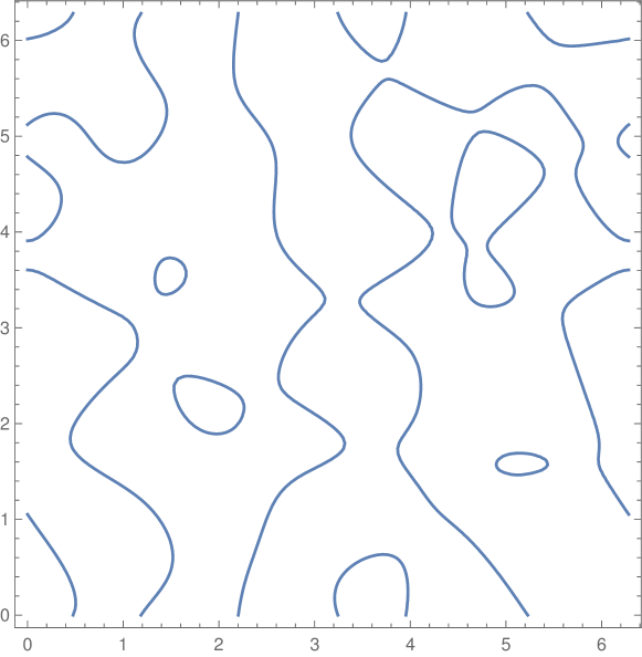
  (a) Bandwidth 2

  

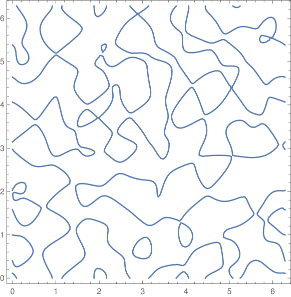
  (b) Bandwidth 4

  

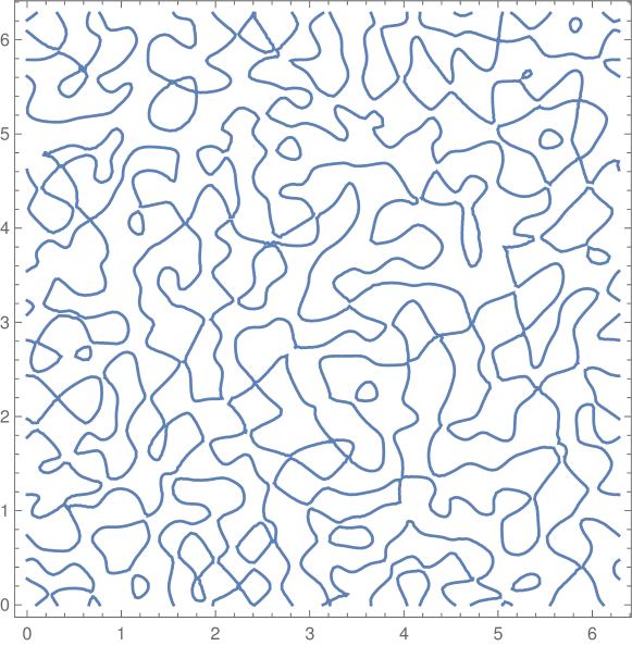
  (c) Bandwidth 8

  

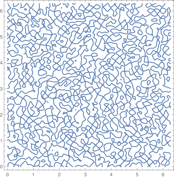
  (d) Bandwidth 16

  Figure 2: Critical curves of bandlimited functions on the flat torus

  We can also verify this linear relationship numerically in Mathematica. For each value of $K$ in $\{2,3,...,10\}$, we choose 20 sets of Fourier coefficients drawn randomly according to the assumptions given in the beginning of this example. We then computed the sample average length of the critical curve for each $K$ and attach the plot in Figure 3. The red points in the plot show the sample average critical curve lengths and the blue line is the best linear fit, which has almost zero y-intercept and is consistent with the observation in (16). The slope of the best fit line is 3.33. We computed the constant $l$ approximately using a sample average with a large number of samples and found it is approximately 0.607, which tells us that $\sqrt{3}\pi l\approx 3.3$. This is very close to the slope of the best fit line in Figure 3.

  Figure 3: Average lengths of critical curves of bandlimited functions

We can compute the average length of the visible contour in a similar fashion as

$$\mathsf{E}\!\left[\vphantom{\big{|}}\operatorname{len}(\gamma_{c})\vphantom{\big{|}}\right]=\frac{\mathsf{E}\!\left[\vphantom{\big{|}}\left|\nabla f^{\top}\operatorname{adj}\left(\nabla^{2}f-\mathsf{E}\!\left[\vphantom{\big{|}}\nabla^{2}f\big{|}\nabla f\vphantom{\big{|}}\right]\right)\nabla f\right|\vphantom{\big{|}}\right]}{2\sqrt{\mathsf{Var}\!\left[\vphantom{\big{|}}\nabla f(x)\vphantom{\big{|}}\right]}},$$ (17)

which becomes

$$\frac{1}{2v_{1}(K)}v_{1}(K)(2K)^{3}\pi^{2}c\approx 4\pi^{2}cK^{3},$$ (18)

where $c=\mathsf{E}\!\left[\vphantom{\big{|}}\left|Z^{\top}MZ\right|\vphantom{\big{|}}\right]$.

• In this example we consider $N$ to be the 2-Torus embedded in $\mathbb{R}^{3}$ in the shape of a hollow doughnut of radius $R$ and cross sectional radius $r$, and the metric to be the metric induced from the Euclidean metric on $\mathbb{R}^{3}$. We denote by $T$ the ratio $\frac{R}{r}$. The embedding can be written in $\phi,\rho$ coordinates as

  $$[0,2\pi]\times[0,2\pi]\ni(\phi,\rho)\mapsto E(\phi,\rho)=\begin{bmatrix}\cos(\phi)\left(R+r\sin(\rho)\right)\\ \sin(\phi)\left(R+r\sin(\rho)\right)\\ r\cos(\rho))\end{bmatrix}\in\mathbb{R}^{3}.$$

  The induced metric tensor can then be written in $(\phi,\rho)$ coordinates as

  $$G(\phi,\rho)=\begin{bmatrix}(R+r\sin(\rho))&0\\ 0&r\end{bmatrix}=\begin{bmatrix}r(T+\sin(\rho))&0\\ 0&r\end{bmatrix}.$$

  We consider random linear projections of this embedding onto $\mathbb{R}^{2}$. That is, we choose $A\in\mathbb{R}^{2\times 3}$ such that each entry is drawn from a standard Gaussian distribution independently of each other, and then define

  $$h(\phi,\rho):=A.E(\phi,\rho)\in\mathbb{R}^{2}.$$

  The two components of $h$ are clearly identical and independent since the two rows of $A$ are i.i.d. and so equations (13) and (14) apply here. We can see that

  $$f(\phi,\rho)=v^{\top}E(\phi,\rho)$$

  where $v$ is drawn from a standard 3D Gaussian distribution. The computations in this example are a bit tedious and are done in Mathematica. We can show that

  $$\mathsf{Var}\!\left[\vphantom{\big{|}}\nabla f(\phi,\rho)\vphantom{\big{|}}\right]=\begin{bmatrix}(R+r\sin(\rho))^{2}&0\\ 0&r^{2}\end{bmatrix}=\begin{bmatrix}r^{2}(T+\sin(\rho))^{2}&0\\ 0&r^{2}\end{bmatrix},$$

  and

  $$\mathsf{Var}\!\left[\vphantom{\big{|}}\begin{bmatrix}f_{\phi,\phi}\\ f_{\phi,\rho}\\ f_{\rho,\rho}\end{bmatrix}\bigg{|}\nabla f=0\vphantom{\big{|}}\right](\phi,\rho)=\left[\begin{smallmatrix}\frac{1}{4}r^{2}(\cos(4\phi)+3)\sin^{2}(\rho)(T+\sin(\rho))^{2}\\ \frac{1}{4}r^{2}\sin(4\phi)\sin^{2}(\rho)\cos(\rho)(T+\sin(\rho))\\ \frac{1}{4}r^{2}(\cos(4\phi)+3)\sin^{3}(\rho)(T+\sin(\rho))\end{smallmatrix}\right.$$

  $$\left.\begin{smallmatrix}\frac{1}{4}r^{2}\sin(4\phi)\sin^{2}(\rho)\cos(\rho)(T+\sin(\rho))&\frac{1}{4}r^{2}(\cos(4\phi)+3)\sin^{3}(\rho)(T+\sin(\rho))\\ \frac{1}{8}r^{2}\sin^{2}(2\phi)\sin^{2}(2\rho)&\frac{1}{4}r^{2}\sin(4\phi)\sin^{3}(\rho)\cos(\rho)\\ \frac{1}{4}r^{2}\sin(4\phi)\sin^{3}(\rho)\cos(\rho)&\frac{1}{32}r^{2}\left((\cos(4\phi)+7)(\cos(4\rho)+3)+8\sin^{2}(2\phi)\cos(2\rho)\right)\end{smallmatrix}\right].$$

  We compute the length of the visible contour when $T\gg 1$. To avoid cumbersome notation, from this point on in this example we will denote $\nabla^{2}f-\mathsf{E}\!\left[\vphantom{\big{|}}\nabla^{2}f|\nabla f\vphantom{\big{|}}\right]$ as just $\nabla^{2}f$. We remind that the variance of this random symmetric matrix is given in the previous equation, and it is independent of $\nabla f$. Observe that

  $$\operatorname{adj}{\nabla^{2}f}=\begin{bmatrix}f_{\rho,\rho}&-f_{\phi,\rho}\\ -f_{\phi,\rho}&f_{\phi,\phi}\end{bmatrix}$$

  and

  $$\nabla f^{\top}(\operatorname{adj}{\nabla^{2}f})\nabla f=f_{\phi}^{2}f_{\rho,\rho}+f_{\rho}^{2}f_{\phi,\phi}-2f_{\phi}f_{\rho}f_{\phi,\rho}.$$

  In addition, $\sqrt{\det{\mathsf{Var}\!\left[\vphantom{\big{|}}\nabla f\vphantom{\big{|}}\right](\phi,\rho)}}=r^{2}(T+\sin(\rho)).$ This random field is not stationary, so we will need to integrate over the torus unlike the previous example. Equation (14) gives us the average length of the visible contour as

  $$\int_{[0,2\pi]}\int_{[0,2\pi]}\frac{\mathsf{E}\!\left[\vphantom{\big{|}}\left|f_{\phi}^{2}f_{\rho,\rho}+f_{\rho}^{2}f_{\phi,\phi}-2f_{\phi}f_{\rho}f_{\phi,\rho}\right|\vphantom{\big{|}}\right]}{2r^{2}(T+\sin(\rho))}d\phi d\rho.$$ (19)

  Observe that

  $$\mathsf{E}\!\left[\vphantom{\big{|}}|f_{\phi}^{2}f_{\rho,\rho}|\vphantom{\big{|}}\right] =\mathsf{E}\!\left[\vphantom{\big{|}}|f_{\phi}^{2}\vphantom{\big{|}}\right]\mathsf{E}\!\left[\vphantom{\big{|}}|f_{\rho,\rho}|\vphantom{\big{|}}\right]=r^{2}(T+\sin(\rho))^{2}\sqrt{\frac{2}{\pi}}\sqrt{\mathsf{Var}\!\left[\vphantom{\big{|}}f_{\rho,\rho}\vphantom{\big{|}}\right]},$$

  $$\mathsf{E}\!\left[\vphantom{\big{|}}|f_{\rho}^{2}f_{\phi,\phi}|\vphantom{\big{|}}\right] =\mathsf{E}\!\left[\vphantom{\big{|}}|f_{\rho}^{2}\vphantom{\big{|}}\right]\mathsf{E}\!\left[\vphantom{\big{|}}|f_{\phi,\phi}|\vphantom{\big{|}}\right]=r^{2}\sqrt{\frac{2}{\pi}}\sqrt{\mathsf{Var}\!\left[\vphantom{\big{|}}f_{\phi,\phi}\vphantom{\big{|}}\right]}$$

  $$=r^{2}(T+\sin(\rho))\sqrt{\frac{2}{\pi}}\sqrt{\frac{\mathsf{Var}\!\left[\vphantom{\big{|}}f_{\phi,\phi}\vphantom{\big{|}}\right]}{(T+\sin(\rho)^{2}}},$$

  $$\mathsf{E}\!\left[\vphantom{\big{|}}|f_{\phi}f_{\rho}f_{\rho,\phi}|\vphantom{\big{|}}\right] =\mathsf{E}\!\left[\vphantom{\big{|}}|f_{\phi}|\vphantom{\big{|}}\right]\mathsf{E}\!\left[\vphantom{\big{|}}|f_{\rho}|\vphantom{\big{|}}\right]\mathsf{E}\!\left[\vphantom{\big{|}}|f_{\phi,\rho}|\vphantom{\big{|}}\right]=\frac{2}{\pi}r^{2}(T+\sin(\rho))\sqrt{\frac{2}{\pi}}\sqrt{\mathsf{Var}\!\left[\vphantom{\big{|}}f_{\phi,\rho}\vphantom{\big{|}}\right]},$$

  where the expectations split as a product because $\nabla^{2}f$ and $\nabla f$ are independent, and we have used the fact that $\mathsf{E}\!\left[\vphantom{\big{|}}|X|\vphantom{\big{|}}\right]=\sqrt{\frac{2}{\pi}\mathsf{Var}\!\left[\vphantom{\big{|}}X\vphantom{\big{|}}\right]}$ for a Gaussian random variable. Clearly, as $T\to\infty$ the $\mathsf{E}\!\left[\vphantom{\big{|}}|f_{\phi}^{2}f_{\rho,\rho}|\vphantom{\big{|}}\right]$ term dominates and we can say that

  $$\mathsf{E}\!\left[\vphantom{\big{|}}\operatorname{len}(\gamma_{c})\vphantom{\big{|}}\right] \approx\int_{[0,2\pi]}\int_{[0,2\pi]}\frac{\mathsf{E}\!\left[\vphantom{\big{|}}\left|f_{\phi}^{2}f_{\rho,\rho}\right|\vphantom{\big{|}}\right]}{2r^{2}(T+\sin(\rho))}d\phi d\rho$$

  $$=\int_{[0,2\pi]}\int_{[0,2\pi]}\frac{(T+\sin(\rho))\sqrt{\mathsf{Var}\!\left[\vphantom{\big{|}}f_{\rho,\rho}\vphantom{\big{|}}\right]}}{\sqrt{2\pi}}d\phi d\rho$$

  $$=\frac{Tr}{\sqrt{2\pi}}\int_{[0,2\pi]}\int_{[0,2\pi]}(1+\frac{\sin(\rho)}{T})\sqrt{\mathsf{Var}\!\left[\vphantom{\big{|}}\frac{f_{\rho,\rho}}{r}\vphantom{\big{|}}\right]}d\phi d\rho,$$

  $$\approx\frac{Rc}{\sqrt{2\pi}}$$

  where

  $$\sqrt{\mathsf{Var}\!\left[\vphantom{\big{|}}\frac{f_{\rho,\rho}}{r}\vphantom{\big{|}}\right]}=\sqrt{\frac{\left((\cos(4\phi)+7)(\cos(4\rho)+3)+8\sin^{2}(2\phi)\cos(2\rho)\right)}{32}}$$

  and

  $$c=\int_{[0,2\pi]}\int_{[0,2\pi]}\sqrt{\mathsf{Var}\!\left[\vphantom{\big{|}}\frac{f_{\rho,\rho}}{r}\vphantom{\big{|}}\right]}d\phi d\rho.$$

  The constant $c$ can be computed numerically as $\approx 31.6$ and so

  $$\mathsf{E}\!\left[\vphantom{\big{|}}\operatorname{len}(\gamma_{c})\vphantom{\big{|}}\right]\approx 12.6R,\quad\text{ when $\frac{R}{r}\gg 1$}.$$ (20)

  A similar computation will show that the length of the critical curve also grows linearly in $R$ when $\frac{R}{r}\gg 1$.

4 Isotropic GRFs on Spheres

All the formulae we computed in the previous section depends only on the joint distribution of $(\nabla f(x),\nabla^{2}f(x))$. When the space $N$ is $\mathbb{S}^{n}$, and the GRF $f$ is isotropic and stationary, we will see that this joint distribution is particularly well structured. Under these conditions, $\nabla f$ and $\nabla^{2}f$ are independent, $\nabla f$ is a standard Gaussian random vector, and $\nabla^{2}f$ is distributed as a Gaussian Orthogonally Invariant (GOI) ensemble. We will see in the following section some of the properties of GOI ensembles that will lead to more reduced formulae for the various computations we did in earlier sections. Most of the results about GOI ensembles mentioned here are a review of what can be found in [CS18].

4.1 Gaussian Orthogonally Invariant Ensembles

An $n\times n$ random matrix $H_{ij}$ is said to have Gaussian Orthogonal Ensemble (GOE) distribution if it is symmetric and all entries are centered Gaussian random variables with

$$\mathsf{E}\!\left[\vphantom{\big{|}}H_{ij}H_{kl}\vphantom{\big{|}}\right]=\frac{1}{2}(\delta_{ik}\delta_{jl}+\delta_{il}\delta_{jk}).$$

It is well known that the GOE ensemble is orthogonally invariant i.e. the distribution of $H$ is the same as that of $QHQ^{\top}$ for any orthogonal matrix $Q$. Moreover, the entries of $H$ are independent. However, we will need a slightly more general distribution to capture the structure of the Hessian of isotropic GRFs.

An $n\times n$ random matrix $M_{ij}$ is said to have Gaussian Orthogonally Invariant distribution with covariance parameter $c$ (GOI(c)) if it is symmetric and all entries are centered Gaussian random variables with

$$\mathsf{E}\!\left[\vphantom{\big{|}}M_{ij}M_{kl}\vphantom{\big{|}}\right]=\frac{1}{2}(\delta_{ik}\delta_{jl}+\delta_{il}\delta_{jk}+c\delta_{ij}\delta_{kl}).$$

The GOI distribution is also orthogonally invariant. In fact, upto a scaling constant any orthogonally invariant symmetric Gaussian random matrix has to have GOI(c) distribution. The only constraint on the covariance parameter is that $c\geq-1/N$ ([CS18, Lemma 2.1]). We will see that the Hessian of isotropic GRFs are GOI ensembles. The orthogonal invariance of GOI random matrices will prove a very useful property in our computations. In addition, the density of the ordered eigenvalues of GOI(c) matrices can be written as

$$f_{c}(\lambda_{1},...,\lambda_{n}) =\frac{1}{K_{n}\sqrt{1+nc}}\exp\left\{-\frac{1}{2}\sum_{i=1}^{n}\lambda_{i}^{2}+\frac{c}{2(1+nc)}\left(\sum_{i=1}^{n}\lambda_{i}\right)^{2}\right\}$$ (21)

$$\times\prod_{1\leq i<j\leq n}|\lambda_{i}-\lambda_{j}|\mathsf{1}\left({\{\lambda_{1}\leq...\leq\lambda_{n}\}}\right)$$

where $K_{n}$ is the normalization constant

$$K_{n}=2^{n/2}\prod_{i=1}^{n}\Gamma\left(\frac{i}{2}\right).$$

For any measurable function $g$, we will denote by

$$\mathsf{E}_{\text{GOI(c)}}^{n}\!\left[\vphantom{\big{|}}g(\lambda_{1},...,\lambda_{n})\vphantom{\big{|}}\right]:=\int_{\mathbb{R}^{n}}g(\lambda_{1},...,\lambda_{n})f_{c}(\lambda_{1},...,\lambda_{n})d\lambda_{1}...d\lambda_{n}$$

the expectation under GOI(c) density.

4.2 Length computations on Isotropic GRFs on spheres

Let $\mathbb{S}^{n}=\left\{(z_{1},..,z_{n+1})\in\mathbb{R}^{n+1}\bigg{|}\sum\limits_{i=1}^{n+1}z_{i}^{2}=1\right\}$ be the unit $n$-sphere embedded in $\mathbb{R}^{n+1}$ endowed with the induced Riemannian metric, and $f$ be a centered, unit-variance, smooth isotropic GRF on $\mathbb{S}^{n}$. Due to isotropy, we can write the covariance function $R$ of $f$ as $R(x,y)=C(\langle x,y\rangle)$ for some $C:[-1,1]\rightarrow\mathbb{R}$. Define

$$C^{\prime}=C^{\prime}(1),C^{\prime\prime}=C^{\prime\prime}(1),\eta=\sqrt{C^{\prime}}/\sqrt{C^{\prime\prime}},\kappa=C^{\prime}/\sqrt{C^{\prime\prime}}.$$

Since an isotropic GRF is also stationary, we only need to compute the integrands in equations (13)-(14) at one point on the sphere. We will choose this point to be the north pole $N=(0,...,0,1)$, and use the fact that $(z_{1},...,z_{n})$ forms a coordinate chart on the sphere in a neighborhood around this point. In this coordinate system, the metric tensor $G(N)$ is simply the identity matrix $I_{n}$. In addition, we have the following lemma giving us the distribution of the derivatives of $f$.

Lemma 4.1.

[CS18, Lemma 4.1, 4.3] Let $f$ be a centered, unit-variance, smooth isotropic GRF on $\mathbb{S}^{n}$. Then

1. $\nabla f$ is $\sqrt{C^{\prime}}$ times a standard Gaussian random vector,

2. $\nabla^{2}f$ is $\sqrt{2C^{\prime\prime}}$ times a GOI($(1+\eta^{2})/2$) matrix,

3. $\nabla f$ and $\nabla^{2}f$ are independent,

where the derivatives are computed in the $(z_{1},...,z_{n})$ coordinates at $N$.

We then have the following result giving a nicer formula for the expected length of the visible contour,

Theorem 4.2.

If $N=\mathbb{S}^{n}$ and the components of the GRF $f$ and $g$ are independent and identically distributed as centered, unit-variance, smooth isotropic GRFs with $C^{{}^{\prime}}\neq 0,C^{{}^{\prime\prime}}\neq 0$, then the expected value of the length of its visible contour of index $k$ is

$$\mathsf{E}\!\left[\vphantom{\big{|}}\operatorname{len}{\gamma_{c}^{k}}\vphantom{\big{|}}\right]=\frac{\sqrt{2\pi^{3}}n}{\Gamma(\frac{n+1}{2})}\frac{\kappa}{\eta^{n}}\mathsf{E}_{\text{GOI$\left(\frac{1+\eta^{2}}{2}\right)$}}^{n-1}\!\left[\vphantom{\big{|}}\prod_{i=1}^{n-1}|\lambda_{i}|\mathsf{1}\left({\lambda_{k}<0<\lambda_{k+1}}\right)\vphantom{\big{|}}\right].$$ (22)

Proof.

Assumption 1.3 is satisfied here, since $(f,\nabla f)$ are independent, $f$ has unit-variance and lemma 4.1 implies $\nabla f$ is non degenerate. Equation (14) gives

$$\mathsf{E}\!\left[\vphantom{\big{|}}\operatorname{len}{\gamma_{c}}\vphantom{\big{|}}\right] =\operatorname{Vol}{(\mathbb{S}^{n})}.\frac{\pi C^{\prime}(\sqrt{2C^{\prime\prime}})^{n-1}}{(\sqrt{2\pi C^{\prime}})^{n}}\mathsf{E}\!\left[\vphantom{\big{|}}\left|v^{\top}\operatorname{adj}(M)v\right|\vphantom{\big{|}}\right]$$

$$=\frac{2\sqrt{\pi^{n+1}}}{\Gamma(\frac{n+1}{2})}\frac{\pi}{\sqrt{2}\sqrt{\pi^{n}}}{\frac{(\sqrt{C^{\prime\prime}})^{n-1}}{(\sqrt{C^{\prime}})^{n-2}}}\mathsf{E}\!\left[\vphantom{\big{|}}\left|v^{\top}\operatorname{adj}(M)v\right|\vphantom{\big{|}}\right]$$

$$=\frac{\sqrt{2\pi^{3}}}{\Gamma(\frac{n+1}{2})}\frac{\kappa}{\eta^{n}}\mathsf{E}\!\left[\vphantom{\big{|}}\left|v^{\top}\operatorname{adj}(M)v\right|\vphantom{\big{|}}\right],$$

where $v$ is a standard unit Gaussian random vector independent of the GOI($\frac{1+\eta^{2}}{2}$) matrix $M$. Since $Q^{\top}\operatorname{adj}(M)Q=\operatorname{adj}(Q^{\top}MQ)$ for any orthogonal matrix $Q$,

$$\mathsf{E}\!\left[\vphantom{\big{|}}\left|v^{\top}\operatorname{adj}(M)v\right|\vphantom{\big{|}}\right] =\mathsf{E}\!\left[\vphantom{\big{|}}\|v\|^{2}\left|(e_{1})^{\top}\operatorname{adj}(R^{\top}MR)e_{1}\right|\vphantom{\big{|}}\right]$$

$$=n\mathsf{E}\!\left[\vphantom{\big{|}}\left|\operatorname{adj}(M)_{11}\right|\vphantom{\big{|}}\right]$$

$$=n\mathsf{E}_{\text{GOI$\left(\frac{1+\eta^{2}}{2}\right)$}}^{n-1}\!\left[\vphantom{\big{|}}\prod_{i=1}^{n-1}|\lambda_{i}|\vphantom{\big{|}}\right],$$

which gives

$$\mathsf{E}\!\left[\vphantom{\big{|}}\operatorname{len}{\gamma_{c}}\vphantom{\big{|}}\right]=\frac{\sqrt{2\pi^{3}}n}{\Gamma(\frac{n+1}{2})}\frac{\kappa}{\eta^{n}}\mathsf{E}_{\text{GOI$\left(\frac{1+\eta^{2}}{2}\right)$}}^{n-1}\!\left[\vphantom{\big{|}}\prod_{i=1}^{n-1}|\lambda_{i}|\vphantom{\big{|}}\right].$$

We can similarly compute the expected length of the critical curve of index $k$ using (14) as

$$\mathsf{E}\!\left[\vphantom{\big{|}}\operatorname{len}{\gamma_{c}^{k}}\vphantom{\big{|}}\right] =\frac{\sqrt{2\pi^{3}}}{\Gamma(\frac{n+1}{2})}\frac{\kappa}{\eta^{n}}\mathsf{E}\!\left[\vphantom{\big{|}}\left|v^{\top}\operatorname{adj}(M)v\right|\mathsf{1}\left({\operatorname{ind}(M)-\mathsf{1}\left({v^{\top}M^{-1}v<0}\right)=k}\right)\vphantom{\big{|}}\right]$$

$$=\frac{\sqrt{2\pi^{3}}}{\Gamma(\frac{n+1}{2})}\frac{\kappa}{\eta^{n}}n\mathsf{E}\!\left[\vphantom{\big{|}}\left|e_{1}^{\top}\operatorname{adj}(Q^{\top}MQ)e_{1}\right|\mathsf{1}\left({\operatorname{ind}(Q^{\top}MQ)-\mathsf{1}\left({e_{1}^{\top}(Q^{\top}MQ)^{-1}e_{1}<0}\right)=k}\right)\vphantom{\big{|}}\right]$$

$$=\frac{\sqrt{2\pi^{3}}n}{\Gamma(\frac{n+1}{2})}\frac{\kappa}{\eta^{n}}\mathsf{E}\!\left[\vphantom{\big{|}}\left|e_{1}^{\top}\operatorname{adj}(M)e_{1}\right|\mathsf{1}\left({\operatorname{ind}(M)-\mathsf{1}\left({e_{1}^{\top}(M)^{-1}e_{1}<0}\right)=k}\right)\vphantom{\big{|}}\right].$$

If we denote by $\hat{M}$ the first $n-1\times n-1$ principal minor of $M$, we can reduce the above expectation as

$$\mathsf{E}\bigg{[} \left|\det(\hat{M})\right|\left(\mathsf{1}\left({\operatorname{ind}(M)=k,(-1)^{k}\det(\hat{M})>0}\right)+\mathsf{1}\left({\operatorname{ind}(M)=k+1,(-1)^{k+1}\det(\hat{M})<0}\right)\right)\bigg{]}.$$

If the index of $M$ is $k$, then the index of $\hat{M}$ can either be $k$ or $k-1$. However, $(-1)^{k}\det(\hat{M})>0$ implies that the index of $\hat{M}$ is $k$. Similarly, if the index of $M$ is $k+1$, then the index of $\hat{M}$ has to be either $k+1$ or $k$, but $(-1)^{k+1}\det(\hat{M})<0$ implies that the the index of $\hat{M}$ is $k$. This allows us to further reduce the above expectation as

$$\mathsf{E}\!\left[\vphantom{\big{|}}\left|\det(\hat{M})\right|\left(\mathsf{1}\left({\operatorname{ind}(M)=k,\operatorname{ind}(\hat{M})=k}\right)+\mathsf{1}\left({\operatorname{ind}(M)=k+1,\operatorname{ind}(\hat{M})=k}\right)\right)\vphantom{\big{|}}\right]$$

$$=\mathsf{E}\!\left[\vphantom{\big{|}}\left|\det(\hat{M})\right|\mathsf{1}\left({\operatorname{ind}(\hat{M})=k}\right)\vphantom{\big{|}}\right].$$

Thus, we can write

$$\mathsf{E}\!\left[\vphantom{\big{|}}\operatorname{len}{\gamma_{c}^{k}}\vphantom{\big{|}}\right] =\frac{\sqrt{2\pi^{3}}n}{\Gamma(\frac{n+1}{2})}\frac{\kappa}{\eta^{n}}\mathsf{E}\!\left[\vphantom{\big{|}}\left|\det(\hat{M})\right|\mathsf{1}\left({\operatorname{ind}(\hat{M})=k}\right)\vphantom{\big{|}}\right]$$

$$=\frac{\sqrt{2\pi^{3}}n}{\Gamma(\frac{n+1}{2})}\frac{\kappa}{\eta^{n}}\mathsf{E}_{\text{GOI$\left(\frac{1+\eta^{2}}{2}\right)$}}^{n-1}\!\left[\vphantom{\big{|}}\prod_{i=1}^{n-1}|\lambda_{i}|\mathsf{1}\left({\lambda_{k}<0<\lambda_{k+1}}\right)\vphantom{\big{|}}\right].$$

∎

5 Expected number of pseudocusps

Pseudocusps can be split into two obvious types, vertical and horizontal, depending on whether they’re the image of critical points of $f$ or $g$ respectively. Recall the notation from section 2; if a point $p$ on $N$ is a critical point of $f$, one can locally parametrize the critical curve in its neighborhood as a function $x(\theta)$ of $\theta$ such that $x(0)=p$. Recall that if

$$V(x,\theta)=\cos(\theta)\nabla f(x)+\sin(\theta)\nabla g(x)=0$$

then the tangent line to the visible contour at $h(x)$ lies along $(-\sin(\theta),\cos(\theta))$. This means the slope of the visible contour at the image of $x(\theta)$ is just $\theta-\frac{\pi}{2}$. For the image of a critical point $p$ to be a vertical pseudocusp, the direction of the tangent vector to the visible contour along the direction of increasing slope must point upward, which means

$$\left\langle\frac{dh(x(\theta))}{d\theta}\bigg{|}_{\theta=0},\ \begin{bmatrix}0\\ 1\end{bmatrix}\right\rangle>0\implies-\nabla g(p)^{\top}\left(\nabla^{2}f(p)\right)^{-1}\nabla g(p)>0.$$

The index of the extension ray attached to a vertical pseudocusp, i.e. the dimension of the cell attached to the sublevel set when the parameter value crosses a point on the extension ray, is just the index of $\nabla^{2}f(p)$. We call this the index of a vertical pseudocusp. The same definition with $g$ replacing $f$ holds for horizontal pseudocusps. Therefore, a vertical pseudocusp of index $k$ is characterized by the conditions

$$\nabla f(p)=0,\ \nabla g(p)^{\top}\left(\nabla^{2}f(p)\right)^{-1}\nabla g(p)<0,\ \operatorname{ind}\left(\nabla^{2}f(p)\right)=k.$$ (23)

while a horizontal pseudocusp of index $k$ is characterized by

$$\nabla g(p)=0,\ \nabla f(p)^{\top}\left(\nabla^{2}g(p)\right)^{-1}\nabla f(p)<0,\ \operatorname{ind}\left(\nabla^{2}g(p)\right)=k.$$ (24)

If $N_{vpc}^{k}$ and $N_{hpc}^{k}$ denote the number of vertical and horizontal pseudocusps of index $k$, the next theorem gives a formula for the expected number of these points.

Theorem 5.1.

If the GRF $h$ satisfies assumptions 1.1-1.3, then the expected number of pseudocusps of index $k$ are

$$\mathsf{E}\!\left[\vphantom{\big{|}}N_{vpc}^{k}\vphantom{\big{|}}\right]=\\ \int_{N}\frac{\mathsf{E}\!\left[\vphantom{\big{|}}\left|\det\left(\nabla^{2}f(p)\right)\right|\mathsf{1}\left({\operatorname{ind}\left(\nabla^{2}f(p)\right)=k,\ \nabla g(p)^{\top}\left(\nabla^{2}f(p)\right)^{-1}\nabla g(p)<0}\right)\bigg{|}\nabla f(p)=0\vphantom{\big{|}}\right]}{\sqrt{(2\pi)^{n}\det\left(\mathsf{Var}\!\left[\vphantom{\big{|}}\nabla f(p)\vphantom{\big{|}}\right]\right)}}dV,$$ (25)

and

$$\mathsf{E}\!\left[\vphantom{\big{|}}N_{hpc}^{k}\vphantom{\big{|}}\right]=\\ \int_{N}\frac{\mathsf{E}\!\left[\vphantom{\big{|}}\left|\det\left(\nabla^{2}g(p)\right)\right|\mathsf{1}\left({\operatorname{ind}\left(\nabla^{2}g(p)\right)=k,\ \nabla f(p)^{\top}\left(\nabla^{2}g(p)\right)^{-1}\nabla f(p)<0}\right)\bigg{|}\nabla g(p)=0\vphantom{\big{|}}\right]}{\sqrt{(2\pi)^{n}\det\left(\mathsf{Var}\!\left[\vphantom{\big{|}}\nabla g(p)\vphantom{\big{|}}\right]\right)}}dV,$$ (26)

Proof.

This is a consequence of the characterizations (25), (26) and the Kac-Rice formula [AT07, Theorem 12.1.1]. ∎

6 Conclusion

We have computed the expected length of the critical curve and visible contour of fixed index of a smooth centered Gaussian random map into the plane in this article. We derived more explicit expressions in the case where the components are identical and independent and a closed form expression under the additional assumption of isotropy. We also computed the expected number of pseudocusps of such a Gaussian random map.

The one remaining singularity appearing in the description of biparametric persistence is the cusp point; these are the points where the visible contour loses smoothness. We have not treated these singularities in this article. The cusps points can be characterized as points where the 2-jet $j^{2}h$ intersects a certain submanifold $S_{1,1}\subset J^{2}(N,\mathbb{R}^{2})$ of codimension $n$. If the support of $j^{2}h(p)$ is full for all $p\in N$, these intersections will be transverse at all $p\in N$ almost surely. We can then compute the expected number of these cusps as the number of transverse intersections of the function $j^{2}h$ with the submanifold $S_{1,1}$ using a generalized Kac-Rice formula [Ste21]. However, these computations are a bit cumbersome and we will pursue these in a future work.

References

- [AA13] Antonio Auffinger and Gerard Ben Arous. Complexity of random smooth functions on the high-dimensional sphere. The Annals of Probability, 41(6):4214–4247, 2013.
- [AAC13] Antonio Auffinger, Gerard Ben Arous, and Jiri Cerny. Random matrices and complexity of spin glasses. Communications on Pure and Applied Mathematics, 66(2):165–201, 2013.
- [APKB21] Mishal Assif P K and Yuliy Baryshnikov. Biparametric persistence for smooth filtrations. arXiv preprint arXiv:2110.09602, 2021.
- [AT07] R. Adler and J. Taylor. Random Fields and Geometry. Springer-Verlag New York, 2007.
- [ATW10] Robert J. Adler, Jonathan E. Taylor, and Keith J. Worsley. Applications of random fields and geometry: Foundations and case studies, 2010.
- [AW09] Jean-Marc Azaïs and Mario Wschebor. Level sets and extrema of random processes and fields. John Wiley & Sons, 2009.
- [BBKS86] James M Bardeen, JR Bond, Nick Kaiser, and AS Szalay. The statistics of peaks of gaussian random fields. The Astrophysical Journal, 304:15–61, 1986.
- [BC21] Peter Bubenik and Michael J Catanzaro. Multiparameter persistent homology via generalized morse theory. arXiv preprint arXiv:2107.08856, 2021.
- [BK21] Ryan Budney and Tomasz Kaczynski. Bi-filtrations and persistence paths for 2-morse functions. arXiv preprint arXiv:2110.08227, 2021.
- [CEF19] Andrea Cerri, Marc Ethier, and Patrizio Frosini. On the geometrical properties of the coherent matching distance in 2D persistent homology. Journal of Applied and Computational Topology, 3(4):381–422, December 2019.
- [CS18] Dan Cheng and Armin Schwartzman. Expected number and height distribution of critical points of smooth isotropic gaussian random fields. Bernoulli, 24(4B):3422, 2018.
- [GG12] Martin Golubitsky and Victor Guillemin. Stable mappings and their singularities, volume 14. Springer Science & Business Media, 2012.
- [LH60] MS Longuet-Higgins. Reflection and refraction at a random moving surface. ii. number of specular points in a gaussian surface. JOSA, 50(9):845–850, 1960.
- [S+20] Michele Stecconi et al. Random differential topology, 2020.
- [Ste21] Michele Stecconi. Kac-rice formula for transverse intersections, 2021.