Exact densities of loops in O(1) dense loop model and of clusters in critical percolation on a cylinder II: rotated lattice.

Abstract

This work continues the study started in [1], where the exact densities of loops in the O(1) dense loop model on an infinite strip of the square lattice with periodic boundary conditions were obtained. These densities are also equal to the densities of critical percolation clusters on the forty five degree rotated square lattice rolled into a cylinder. Here, we extend those results to the square lattice with a tilt. This in particular allow us to obtain the densities of critical percolation clusters on the cylinder of the square lattice of standard orientation extensively studied before. We obtain exact densities of contractible and non-contractible loops or equivalently the densities of critical percolation clusters, which do not and do wrap around the cylinder respectively. The solution uses the mapping of O(1) dense loop model to the six-vertex model in the Razumov-Stroganov point, while the effective tilt is introduced via the the inhomogeneous transfer matrix proposed by Fujimoto. The further solution is based on the Bethe ansatz and Fridkin-Stroganov-Zagier’s solution of the Baxter’s T-Q equation. The results are represented in terms of the solution of two explicit systems of linear algebraic equations, which can be performed either analytically for small circumferences of the cylinder or numerically for larger ones. We present exact rational values of the densities on the cylinders of small circumferences and several lattice orientations and use the results of high precision numerical calculations to study the finite-size corrections to the densities, in particular their dependence on the tilt of the lattice.

1 Introduction

Percolation is a classical problem used as a testing ground of the theory of critical phenomena. It is formulated in terms of a graph, in which bonds (for bond percolation) or sites (for site percolation) are independently selected to be either open or closed with fixed probabilities $\tt{p}$ and $(1-\tt{p})$ respectively. The adjacent open bonds or sites form connected clusters. The hallmark of the percolation at infinite graphs is a phase transition: an infinite connected component arise at a critical point $\tt{p}=\tt{p}_{c}$. A significant effort has been paid to study this phase transition [2, 3, 4]. In particular, the density (the mean per site number) of connected clusters, is one of simplest quantities that have been studied for a long time. This is the main subject of the present paper.

A biggest progress in calculation of the cluster densities has been made for the most analytically tractable non-trivial example of percolation, percolation on two-dimensional periodic planar lattices. In early history the cluster densities were investigated with the help of series expansions, which in particular allowed the use of duality arguments to find critical points for percolation in several lattices [5, 6]. A significant advance was achieved for the critical, $\tt{p}=\tt{p}_{c}$, bond percolation on the square lattice and triangular lattices for them being exactly solvable with the toolbox of the theory of integrable systems [7]. In particular the exact values of the infinite plane limit of critical percolation cluster densities were obtained [8, 9].

These limits, however, being model dependent quantities are not universal characteristics of the percolation phase transition. On the other hand, the scaling limit of the critical percolation in two dimensions is believed to enjoy the conformal invariance that, in particular, was rigorously proved for the site percolation on the triangular lattice [10]. To see manifestation of conformal invariance in the cluster densities one can consider percolation in a restricted geometry, e.g. on the infinite lattice strip of a finite width. The conformal field theory (CFT) predicts universal finite size corrections to the bulk values of the cluster densities, which depend on the boundary conditions on the boundaries of the strip. They are given by the conformal anomalies [11] that were found from using both the Bethe ansatz solution of related models [12, 13] or the Coulomb gas theory [14]. The CFT based leading finite size corrections to critical percolation cluster densities were conjectured and numerically checked in [15, 16].

The mentioned results characterize the asymptotic behavior of cluster densities on a strip in the large strip width limit. On the other hand, the question about exact values of the cluster densities on strips of an arbitrary finite width is still open even for the simplest planar lattices like square and triangular lattice. Their explicit expressions would allow one not only to obtain the leading universal finite size corrections, but also to study the next terms of the asymptotic expansion in the inverse strip width, which might also have a interesting CFT content.

The dependence of the densities of percolation clusters on the open bond probability $\tt{p}$ was studied in [17, 18] for lattice strips of finite width. Unfortunately, the integrability toolbox can not be used for general values $\tt{p}$. Therefore, only a few small values of the strip width were treated, for which the problem is reduced to manipulations with the finite dimensional transfer matrix. No generalization for arbitrary lattice sizes is known to be achievable in this way.

Here we are going to apply an integrability based approach to study the critical, $\tt{p}=\tt{p}_{c}=1/2$, percolation cluster densities on the strip wrapped into a cylinder with boundary conditions specified below. To this end, we note that the percolation problem can alternatively be formulated in different languages, e.g. as particular limits of Potts model or random cluster model that in turn can be related to the $O(n)$ dense loop model (DLM) [7]. The O(n) DLM on the square lattice is defined as an ensemble of weighted non-crossing paths passing through every bond and making a ninety degree turn at every site, so that every closed loop brings the weight $n$. In particular, the critical bond percolation model on the square lattice can be mapped to the O(1) DLM on another square lattice that is a so called medial graph of the original lattice. Conversely, given a loop configuration on the square lattice, we can recover the percolation cluster configuration on the forty five degree rotated square lattice with vertices associated with half of faces of the original lattice arranged in the checkerboard pattern. In particular, the original lattice (with loops) wrapped into a cylinder of even circumference corresponds to the rotated one (with percolation clusters) also wrapped into a cylinder, see fig. 1. Thus, instead of studying the statistics of percolation clusters, one can equivalently study the statistics of loop configurations. Specifically, as we explain later, the critical percolation cluster density is equal to the density of loops on the medial lattice.

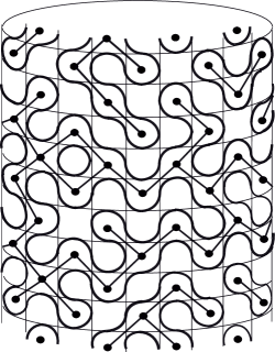
Figure 1: Loop configuration of O(1) DLM on the square lattice wrapped into a cylinder and corresponding percolation clusters on the forty five degree rotated lattice.

The solvability of the $O(1)$ DLM on the square lattice is due to its connection with the Bethe ansatz solvable six vertex model [7, 8, 19]. In particular, a special point of its parameter space related to O(1) DLM is the so called Razumov-Stroganov point, distinguished by a remarkable combinatorial structure of the ground state eigenvector of the six vertex transfer matrix or of the related XXZ Hamiltonian [20]. It is this point that is responsible for a possibility of obtaining exact finite size formulas for the ground state observables of the model. Indeed, connections between the percolation, the $O(1)$ DLM, the six vertex model, the XXZ model, the fully packed loop model and alternating sign matrices [21, 22, 23, 24] yielded plenty conjectures and exact results for finite lattices with various boundary conditions [25, 26, 27, 28, 29, 30, 31, 32, 33, 34, 35].

However, the exact densities of loops in O(1) DLM and related critical percolation cluster densities had not been studied until recently. In a recent letter [1] we considered the $O(1)$ dense loop model (DLM) on an infinite the square lattice cylinder of even circumference. Note that in the cylinder geometry one can distinguish between two types of loops, contractible and non-contractible ones, that can be given their own fugacities within the mapping to the six vertex model [36]. Thus, the exact densities of contractible and non-contractible loops, which also gave the densities of the critical percolation clusters on the forty-five degree rotated lattice, were obtained. We showed that these densities are given by explicit rational functions of the circumference of the cylinder. At large circumference, the leading and sub-leading orders of their asymptotic expansion reproduced the previous asymptotic results.

The densities obtained, however, can not be directly compared to most of the results on percolation available to date, e.g. those of [17, 18], since the latter are obtained for the percolation on the cylinder with standard lattice orientation, which conversely would correspond to O(1) DLM on forty five degree rotated lattice. In general, the infinite plane limit of the cluster densities on the cylinder does not depend on the lattice orientation, and the form of leading finite size correction to this limit is expected to be universal, i.e. to depend on the lattice orientation only via the length rescaling. At the same time, the exact values of critical percolation cluster densities and, in particular, the next to sub-leading finite size corrections do depend on the lattice orientation. This dependence is the subject of the present article.

Below we continue the studies started in [1] carrying out calculations of the densities of contractible and non-contractible loops in $O(1)$ DLM on the cylinder obtained from the square lattice rotated by an angle $\alpha$, such that $\tan\alpha=m/n$ is a rational number indexed by two co-prime integers $m\leq n$. Correspondingly they yield the densities of critical percolation clusters on the cylinder of the square lattice rotated by the angle $\alpha+\pi/4$ with respect to the standard orientation. In particular, when $\alpha=\pi/4$, corresponding to $(n,m)=(1,1)$, we obtain the cluster densities for the standard lattice orientation, which can be compared with previous results.

The solution is based on the mapping of the $O(1)$ DLM to the six-vertex model [19]. To introduce the tilt into the lattice we apply the trick proposed in [37], see also [38], that consists in use of the transfer matrix of inhomogeneous six vertex model, which effectively replaces part of the vertices of the lattice by a pair of non-interacting bonds. As a result, we arrive at the T-Q equation, the solution of which at the Razumov-Stroganov point can be represented in terms of the solution of an explicit linear system. Then, the densities of clusters given by the derivatives of the largest eigenvalue of the transfer matrix with respect to parameters is expressed in terms of the Q-operator and the P-operator that solves a conjugated T-P equation. The technique based on the interplay between P- and Q- operators comes back to Pronko and Stroganov [39] (see also [40] for the case with a twist). The method of exact solution of T-Q and T-P equations at the Razumov-Stroganov point and of calculating derivatives of the largest eigenvalue with respect to the loop fugacities was developed by Fridkin, Stroganov, Zagier in [41, 42]. Our calculations follow the line of [1] based on those two papers.

Unlike [1], here we were not able to express the Q- and P-operators in terms of hypergeometric (or any other special) functions. This is why the final result does not have an explicit functional form. Rather it is given in terms of the solution of the linear system. For a finite circumference of the cylinder it can be solved using the Wolfram Mathematica, and yields explicitly exact rational values of the densities for the circumferences as small as a few tens and not too big values of $m$ and $n$. The approximate decimal values of the densities calculated with arbitrarily high numerical precision are available for much bigger sizes of the densities. We use the decimal approximation to study the tilt dependence of the finite size corrections to the densities.

The article us organized as follows. In section 2 we introduce the O(1) DLM, critical percolation model and the six-vertex model on the tilted lattice, and explain connections between them. Then, we formulate a problem of finding the specific free energy for these models, from which the densities of loops and clusters can be obtained as its derivatives. In Section 3 we derive T-Q and T-P equations and show how the derivatives of the free energy can be obtained from Q- and P-operators. In Section 4 we give solutions for Q- and P-operators in terms of the solution of an explicit system of linear algebraic equations and use them to derive the final formulas for the densities. Section 5 contains final results on exact rational values of the densities for small lattices and asymptotic analysis of results of numerical solution, which demonstrate conformal invariance of the sub-leading finite size corrections and leads us to conjectures on the form of the non-universal next to sub-leading finite size corrections to the density.

2 O(1) DLM, percolation and six-vertex model on a tilted lattice.

Let us fix two non-negative co-prime integers $m,n\in\mathbb{N}_{0}$, which are not zero simultaneously, and positive integer $l\in\mathbb{N}$, such that

$$L=(m+n)l\in 2\mathbb{N}$$ (1)

is an even positive integer. Though we can consider arbitrary $n,m$ and $l$ such that $L$ is even, transferring factors between the first two and the third one as well as swapping $n$ and $m$ results in equivalent situations.Therefore it is enough to limit our choice to co-prime $m\leq n$ and arbitrary $l$.

Consider a strip of the square lattice $\mathcal{L}=(V,E)$ with vertex set $V=\{1,\dots,ln\}\times\mathbb{Z}$ and edge (or bond) set $E=\{(v,v+\boldsymbol{e}_{x}),(v,v+\boldsymbol{e}_{y}))\}_{v\in V}$, where $\boldsymbol{e}_{x}=(1,0)$ and $\boldsymbol{e}_{y}=(0,1)$ are lattice vectors, rolled into a cylinder with helical boundary conditions (BC), i.e. we imply that $v\equiv v+nl\cdot\boldsymbol{e}_{x}-ml\cdot\boldsymbol{e}_{y}$ for any $v\in V$. The helical BC introduce a tilt with angle $\alpha$, such that $\tan\alpha=m/n$. The $O(1)$ DLM on this lattice is formulated as a measure on path configurations, in which a path passes through every bond exactly once, and two paths meet at every site without crossing each other. All the path configurations on any finite part of the lattice have equal weights.

The path configurations can be constructed with local operations by placing one of two vertices at every lattice site, in which two pairs of paths at four incident bonds are connected pairwise in one of two possible ways shown in fig. 2, both assigned with the unit weight.

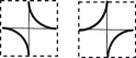
Figure 2: Two vertices of the O(1) loop models. Both vertices have unit weight.

The choice of even $L$ ensures that under the uniform measure on paths only finite closed loops present on the cylinder with probability one, each loop having the weight $w=1$.

The loop configurations are in one to one correspondence with the set of open and closed bonds on the lattice $\mathcal{L}^{\prime}$, for which the original lattice is the medial graph, i.e. sites of $\mathcal{L}^{\prime}$ are placed to the center of every second face of $\mathcal{L}$ in a staggered way and bonds are passing through the nearest sites of $\mathcal{L}$, see fig. 4. The helical boundary conditions for $\mathcal{L}$ suggest that $\mathcal{L}^{\prime}$ is also a cylinder rolled out of the strip of the square lattice, but with the tilt $\alpha^{\prime}=\alpha+\pi/4$. In particular the choice $(n,m)=(1,1)$ suggests that $\alpha^{\prime}=\pi/2$, i.e. $\mathcal{L}^{\prime}$ is the square lattice in the standard orientation. Then, a bond of $\mathcal{L}^{\prime}$ is open (closed), when it is between (crosses) the loop arcs, see fig. 3. The probability of an open bond is $1/2$ as well as of a closed one. This is the critical point of the bond percolation on the infinite square lattice.

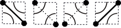
Figure 3: Correspondence between the vertices of O(1) DLM at $\mathcal{L}$ and open (solid) or closed (dashed) bonds on $\mathcal{L}^{\prime}$. The black dots are sites of $\mathcal{L}^{\prime}.$

Figure 4: Loops on the part of infinite cylinder rolled out of a tilted lattice with $(m,n)=(3,1)$ and associated percolation clusters on the lattice rotated by $\pi/4$. Contractible and non-contractible loops are shown in blue and red respectively. The green dots on the left and right hand sides mark the faces (and the sites if the rotated lattice), which are identified when the strip is rolled into the cylinder.

We use the notations $\nu_{\mathrm{c}}(l,m,n)$ and $\nu_{\mathrm{nc}}(l,m,n)$ for the densities, i.e. average per site numbers, of contractible and non-contractible loops, respectively. Similarly to [1] they are also the densities of percolation clusters that do not and do wrap around the cylinder $\mathcal{\mathcal{L}}^{\prime}$ respectively. This is obvious for non-contractible loops since every percolation cluster wrapped around the cylinder on $\mathcal{L}^{\prime}$ is surrounded by two non-contractible loops on $\mathcal{L}$, while $\mathcal{L}^{\prime}$ contains twice less sites per unit length of the cylinder than $\mathcal{L}$. For contractible loops, we note that every contractible loop is either circumscribed on a percolation cluster that does not wrap around the cylinder or is inscribed into a hole inside a percolation cluster. The latter loop can also be thought of as circumscribed on the dual percolation cluster on the lattice dual to $\mathcal{L}^{\prime}$. The critical point is self-dual. This means that the average numbers of percolation clusters and of dual percolation clusters are equal, and so are the average numbers of the circumscribed and the inscribed loops.

To proceed with the analytic solution we exploit the relation of $O(1)$ DLM with the six-vertex model going first to the directed loop model [19] by giving either clockwise or counterclockwise orientation to every loop. This makes the arcs within the vertices in fig. 2 directed, which is indicated by an arrow, fig. 5. Then, attaching arrows to bonds incident to every site consistently with the directions of the arcs and ignoring the connectivities we obtain six vertices of the six-vertex model out of eight vertices of the directed loop model.

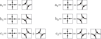
Figure 5: Correspondence between the six-vertex model and the directed loop model.

To define the model on the strip of even width $L$ of standard orientation square lattice rolled into a cylinder we assign the following weights to the vertices

$$a_{1} = \frac{u^{1/2}-u^{-1/2}}{q^{-1/2}-q^{1/2}}e^{\mathrm{i}\frac{\varphi}{L}},\quad a_{2}=\frac{u^{1/2}-u^{-1/2}}{q^{-1/2}-q^{1/2}}e^{-\mathrm{i}\frac{\varphi}{L}},$$ (2)

$$b_{1} = \frac{q^{-1}u^{-1/2}-qu^{1/2}}{q^{-1/2}-q^{1/2}}e^{\mathrm{i}\frac{\varphi}{L}},\quad b_{2}=\frac{q^{-1}u^{-1/2}-qu^{1/2}}{q^{-1/2}-q^{1/2}}e^{\mathrm{-i}\frac{\varphi}{L}},$$ (3)

$$c_{1} = q^{1/2}+q^{-1/2},\quad c_{2}=q^{1/2}+q^{-1/2}.$$ (4)

This is one of standard parametrizations of the weights of six-vertex model [43]. Then, at a special value of the spectral parameter $u=1/q$ the weight of clockwise (counterclockwise) quarter turn of a directed loop is given by $q^{1/4}$ ($q^{-1/4}$) and the weight of the right (left) horizontal step is $e^{\mathrm{i}\varphi/L}$ ($e^{-\mathrm{i}\varphi/L}$). As a consequence, the weights of contractible and non-contractible undirected loops are given by

$$w_{\mathrm{c}}=2_{q}=q+q^{-1}\quad\mathrm{and}\quad w_{\mathrm{n}c}=2\cos\varphi$$ (5)

respectively becoming the unit weights, $w_{\mathrm{c}}=w_{\mathrm{n}c}=1,$ in the so called stochastic point

$$q=e^{\frac{\mathrm{i}\pi}{3}},\quad\varphi=\pi/3.$$ (6)

Let us define the $R$-matrix

$$R(u)=\left(\begin{array}[]{cccc}a_{1}&0&0&0\\ 0&b_{1}&c_{1}&0\\ 0&c_{2}&b_{2}&0\\ 0&0&0&a_{2}\end{array}\right)$$ (7)

and its analogues acting in the tensor product of $L+1$ two-dimensional spaces $R_{ij}(u)\in\mathrm{End}\left(\mathbb{C}^{2}\right)^{\otimes(L+1)}$, which act as $R(u)$ in the pair of spaces $i$ and $j$ and identically in the others. Such defined $R-$matrices satisfy the following Yang-Baxter equation

$$R_{12}\left(q^{-2}u/v\right)R_{13}\left(u\right)R_{23}\left(v\right)=R_{23}\left(v\right)R_{13}\left(u\right)R_{12}\left(q^{-2}u/v\right).$$ (8)

As was noted above, to construct the transfer matrix for the model on the lattice in the standard orientation it would be enough to use a particular specialization $R(1/q)$ of the $R$-matrix, which we will refer to as normal vertices.

It was shown in [37, 38] that the use of auxiliary vertices obtained from other specializations allows one to introduce an effective tilt into the lattice. Note, that first solution of the problem of six-vertex model on the rotated lattice was given in [44] using the method based on the random walk representation of the Bethe ansatz. Here, we follow [45], where the Reader can consult about the details of the further construction.

To define the tilted model, we first note that two other specializations of the $R$-matrix

$$R(1)=\left(q^{1/2}+q^{-1/2}\right)\left(\begin{array}[]{cccc}0&0&0&0\\ 0&e^{\mathrm{i}\frac{\varphi}{L}}&1&0\\ 0&1&e^{-\mathrm{i}\frac{\varphi}{L}}&0\\ 0&0&0&0\end{array}\right)$$ (9)

and

$$R\left(q^{-2}\right)=\left(q^{1/2}+q^{-1/2}\right)\left(\begin{array}[]{cccc}e^{\mathrm{i}\frac{\varphi}{L}}&0&0&0\\ 0&0&1&0\\ 0&1&0&0\\ 0&0&0&e^{\mathrm{-i}\frac{\varphi}{L}}\end{array}\right)$$ (10)

can be treated as vertices with pairs of arcs connecting either west to south and north to east or west to north and east to south, see fig. 6.

Figure 6: The auxiliary vertices.

Up to the overall extra factor $(q^{1/2}+q^{-1/2})$ the matrix elements corresponding to unit weight vertices with fixed connectivity are also supplied with factors $e^{\pm\mathrm{i}\varphi/L},$ which account for the left-right arrow propagation.

Given $n,m,l$ and $L$ defined in (1), we introduce a one-parametric family of commuting transfer matrices

$$V(u)=\mathrm{Tr}_{0}\prod_{i=0}^{l-1}\left(\prod_{j=il+1}^{il+m}R_{0j}\left(\frac{u}{q}\right)\prod_{k=il+m+1}^{il+m+n}R_{0k}(u)\right),$$ (11)

which are operators acting in the tensor product of $L$ two-dimensional “quantum” spaces, $V(u)\in\mathrm{End}\left(\mathbb{C}^{2}\right)^{\otimes L}$, with indices $1,\dots,L$, while the auxiliary space with index $0$ has been traced out. The commutativity of the transfer matrices at different values of the spectral parameter,

$$[V(u),V(v)]=0,$$

can be proved using the Yang-Baxter equation (8).

Thus, there are $l$ groups of $m$ auxiliary vertices of type (10) alternating with $l$ groups of $n$ normal vertices in $V(1/q)$. Likewise, $V(1)$ contains $l$ groups of $m$ normal vertices alternating with $l$ groups of $n$ auxiliary vertices of type (9).

Concatenating groups of $n$ rows of the lattice of type $V(1/q)$ alternatingly with groups of $m$ rows of type $V(1)$ and letting the number of rows of the lattice to be $(m+n)l^{\prime}$ with some $l^{\prime}\in\mathbb{N}$ we define partition function

$$Z_{n,m,l,l^{\prime}}(q,\varphi)=\mathrm{Tr}_{1,\dots,L}\left[\left(V(1/q)\right)^{n}\left(V(1)\right)^{m}\right]^{l^{\prime}}\left(q^{1/2}+q^{-1/2}\right)^{-2mnll^{\prime}}.$$ (12)

which is nothing but the torus partition function of the loop model on the inhomogeneous lattice with some vertices replaced by a pair of non-interacting arcs, while contractible and non-contractible loop weights are still as in (5). One can see in fig. 7 that the new lattice obtained by introducing the split vertices is equivalent to the tilted lattice, while the periodic boundary conditions turn into the helical boundary conditions described in the beginning of the section.

Figure 7: Transformation of the lattice by introducing the auxiliary vertices split into two non-interacting arcs. The example shown corresponds to $(n,m)=(2,1)$ and $l=2$. The cuts in split vertices corresponding to $R(1/q^{2})$ and $R(1)$ are shown by $/$ and $\backslash$ respectively on the leftmost picture, while the usual vertices correspond to $R(1/q)$. The split vertices are replaced by pairs of arcs in picture in the center. The stretch of the central picture converts it to the piece of the tilted square lattice on the right. The left and right black squares on the same horizontal level are identified under imposing periodic boundary due to the trace in (11). The strip between two dashed horizontal lines on the left and central pictures becoming the zig-zag-like strip in the right one corresponds to the transfer matrix $(V(1/q))^{n}(V(1))^{m}$ that acts between two spaces depicted by the dashed lines. The strips are concatenated repeatedly $l^{\prime}$ times in the vertical direction and the first space is identified with the last space within the partition function (12).

Here, the second factor compensates for the extra weight coming from $2mnll^{\prime}$ auxiliary vertices. Now we define the per site free energy of the model on infinite cylinder, obtained by letting $l^{\prime}\to\infty,$

$$f_{n,m,l}(w_{\mathrm{c}},w_{\mathrm{n}c})=\lim_{l^{\prime}\to\infty}\frac{\log Z_{n,m,l,l^{\prime}}(q,\varphi)}{\left(m^{2}+n^{2}\right)ll^{\prime}},$$ (13)

that is a function of the loop weights defined in (5) as well as of the parameters $n,m$ and $l$. Here the denominator $\left(m^{2}+n^{2}\right)ll^{\prime}$ is the number of normal vertices out of the total number $(m+n)^{2}ll^{\prime}$ of the vertices. In particular the contractible and non-contractible loop densities are given by

$$\nu_{\mathrm{c}}(l,m,n) = \left.w_{\mathrm{c}}\frac{\partial}{\partial w_{\mathrm{c}}}\right|_{w_{\mathrm{c}},w_{\mathrm{n}c}=1}f_{n,m,l}(w_{\mathrm{c}},w_{\mathrm{n}c}),$$ (14)

$$\nu_{\mathrm{nc}}(l,m,n) = \left.w_{\mathrm{nc}}\frac{\partial}{\partial w_{\mathrm{n}c}}\right|_{w_{\mathrm{c}},w_{\mathrm{n}c}=1}f_{n,m,l}(w_{\mathrm{c}},w_{\mathrm{n}c}).$$ (15)

To evaluate the free energy we note that the limit in (13) is governed by the largest eigenvalue of the transfer matrix (11). To identify the largest eigenvalue we first note that the space $\mathcal{H}=\left(\mathbb{C}^{2}\right)^{\otimes L}$, where the transfer matrix $V(u)$ acts, is a span of the basis consisting of $2^{L}$ vectors of the form $\otimes_{i=1}^{L}e^{(k_{i})}_{i}$, where a factor $e^{(k_{i})}_{i}$ with the superscript $k_{i}\in\{0,1\}$ is one of the vectors $e^{(0)}=(0,1)^{T}$ or $e^{(1)}=(1,0)^{T}$ and the running subscript $i$ indexes the spaces within the tensor product. Such basis vectors represent possible states of $L$ vertical bonds on the same horizontal level of the lattice with up or down arrow corresponding to $e^{(0)}$ and $e^{(1)}$ respectively. Then, the whole space $\mathcal{H}$ is decomposed into $L+1$ invariant sub-spaces $\mathcal{H}=\oplus_{p=0}^{L}\mathcal{H}_{p}$, where each $\mathcal{H}_{p}$ stable under the action of $V(u)$ is a span of the basis vectors with fixed number $p=0,\dots,L$ of up arrows. Then, the question is in which subspace the eigenstate corresponding to the largest eigenvalue lives and whether it is unique.

The first answer to this question applied to variants of the symmetric six vertex model was given in Lieb’s seminal solution of the ice, KDP and F models [46, 47, 48, 49] based on the results of Yang and Yang [50, 51] for the related XXZ chain. In particular, Lieb established that in the disordered phase, $-1<\Delta<1$, of the symmetric six-vertex model on the cylinder of circumference $L$ the dominant eigenstate belongs to the invariant subspace $\mathcal{H}_{p}$ with $p=p_{\max}$ asymptotically equal to $L/2$, i.e. $p_{\max}/L\to 1/2$ as $L\to\infty$. Furthermore, in that case the transfer matrix restricted to a subspace $\mathcal{H}_{p}$ with any $p$ is irreducible and aperiodic with real non-negative coefficients, i.e. satisfying conditions of the Perron-Frobenius theorem. Hence, the maximal eigenstate in each invariant subspace is the Perron-Frobenius eigenvector, which is non-degenerate with strictly positive components. This is true in particular for the maximal over all the invariant sub-spaces eigenvalue. To our knowledge, the statement about $p_{\max}$ is still proved rigorously only asymptotically, see e.g. [52], though a commonly believed conjecture is that a stronger statement can be made that holds for finite $L$. In particular, the non-degenerate largest eigenvalue is expected to be found in the subspace with $p=p_{\max}=L/2$ for even finite $L$.

In our notations, the symmetric six vertex model in the disordered phase with $\Delta=-(q+q^{-1})/2$ corresponds to the weights (2-4) with $\varphi=0$ and $|q|=|u|=1$ under constraints $0<\arg q<\pi$ and $0<2\arg q+\arg u<2\pi$, which ensure non-negativity of Boltzmann weights. Thus, it would be natural to expect that the properties mentioned are preserved by continuity at least in some vicinity of $\varphi=0$, though at nonzero $\varphi$ the transfer matrix is not real valued anymore. In fact, the situation turns out even better at the stochastic point (6) exactly due to its connection with O(1) DLM that can effectively be formulated as a Markov chain, of which the dominant eigenstate is simply a stationary state. The rough idea is to consider the transfer matrix of the homogeneous six vertex model in a different basis that was constructed in [33, 25, 28]. In this basis the six vertex transfer matrix turns into a real valued symmetric O(1) DLM transfer matrix that adds a row of vertices from fig. 2 on top of the semi-infinite cylinder. These basis vectors record how the vertical terminal bonds are connected to one another by half-loops within the semi-infinite cylinder. Thus, they are indexed by non-crossing pairings the of $L$ points on the rim of punctured annulus and the basis spans the subspace $\mathcal{H}_{p}$ with $p=L/2$ of the arrow basis of the six-vertex model, while the other sub-spaces are related with the loop configurations containing defect lines and are suppressed in the infinite system. In this setting the dominant eigenstate is the Perron-Frobenius eigenvector with the eigenvalue that is non-degenerate and thus analytic in its parameters at least in a vicinity of the stochastic point. In fact, as far as spectral parameter $u$ varies in a range of values of $u$, which preserves the conditions of the Perron-Frobenius theorem, the largest eigenvalue remains non-crossing and the dominant eigenstate does not change being independent of $u$. See [33, 25, 28] for further details.

The same construction is readily applied to our tilted transfer-matrix. Specifically, the largest eigenvalue of $V(u)$ is a Perron-Frobenius eigenvalue in the range $-\pi/3\leq\arg u\leq 0$, i.e. it is non-degenerate and thus analytic in $q$ and $\varphi$ in a vicinity of stochastic point (6) and the largest eigenstate belongs to the subspace $\mathcal{H}_{L/2}$. Taking into account (11,12,13), the fact that the commuting transfer matrices are diagonalizable or at least can be brought to the Jordan form in the same basis and also share the same non-degenerate dominant eigenvector, we express the free energy in terms of the largest eigenvalue $\Lambda_{\max}(u)$ of the transfer matrix $V(u)$

$$f_{n,m,l}(w_{\mathrm{c}},w_{\mathrm{n}c})=\frac{n\log\Lambda_{\max}(1/q)+m\log\Lambda_{\max}(1)}{\left(m^{2}+n^{2}\right)l}-\frac{2nm\log\left(q^{1/2}+q^{-1/2}\right)}{m^{2}+n^{2}}.$$ (16)

The next step of our program is to evaluate $\Lambda_{\max}(u)$ and its derivatives with respect to $q$ and $\varphi$.

3 Bethe ansatz, T-Q, T-P and Q-P relations.

The standard technique of solution of the eigenvalue problem for the transfer matrix of the six-vertex model is the algebraic Bethe ansatz. The Bethe ansatz provides a recipe of construction of eigenstates starting from the vacuum state with only down arrows. Omitting standard though technical details that can be found e.g. in [53], we arrive at the following expression of the eigenvalue under assumption that corresponding eigenstate belongs to the subspace $\mathcal{H}_{p}\subset\mathcal{H}$ with $p=0,\dots,L$ up arrows

$$\Lambda(u) =\frac{e^{\mathrm{i}\varphi}}{(-q)^{p}}\left(\frac{\left(u/q\right)^{1/2}-\left(q/u\right)^{1/2}}{q^{-1/2}-q^{1/2}}\right)^{ml}\left(\frac{u^{1/2}-u^{-1/2}}{q^{-1/2}-q^{1/2}}\right)^{nl}\prod_{k=1}^{p}\frac{q^{2}u-u_{k}}{u-u_{k}}$$

$$+\frac{e^{\mathrm{-i}\varphi}}{(-q)^{p}}\left(\frac{\left(uq\right)^{-1/2}-\left(uq\right)^{1/2}}{q^{-1/2}-q^{1/2}}\right)^{ml}\left(\frac{\left(u^{1/2}q\right)^{-1}-\left(u^{1/2}q\right)}{q^{-1/2}-q^{1/2}}\right)^{nl}\prod_{k=1}^{p}\frac{u-q^{2}u_{k}}{u-u_{k}},$$

where $u_{1},\dots,u_{p}$ are the roots of the system of Bethe ansatz equations (BAE)

$$e^{2\mathrm{i}\varphi}\left(\frac{u_{i}-q}{1-qu_{i}}\right)^{ml}\left(\frac{u_{i}-1}{q^{-1}-qu_{i}}\right)^{nl}=\left(-1\right)^{p-1}\prod_{k\neq i;k=1}^{p}\frac{u_{i}-q^{2}u_{k}}{u_{k}-q^{2}u_{i}}.$$ (18)

The system (18) is exactly the condition of $\Lambda(u)u^{(n+m)l/2}$ being polynomial in $u$, which follows from the structure of the weights (2-4).

Let us rephrase it in a more convenient way. First we note that the largest eigenvalue we are interested in is known to belong to the sector with

$$p=\frac{L}{2}=\frac{l(n+m)}{2}.$$

Thus, from now on we will assume this value of $p.$

For convenience we introduce the following function

$$T(u)=\Lambda(u)u^{p}q^{-p-nl/2}(-1)^{p}(1-q)^{L},$$ (19)

which is expected to be a polynomial in $u$ of degree at most $L$. We also introduce Q-polynomial

$$Q(u)=\prod_{i=1}^{p}(u-u_{k}),$$

of degree $p$ with roots being the Bethe roots from the solution of (18) corresponding to the largest eigenvalue. Then (3) can be rewritten in the form of T-Q equation

$$T(u)Q(u)=e^{\mathrm{i}\varphi}\Phi\left(uq^{-1}\right)Q(uq^{2})+e^{-\mathrm{i}\varphi}\Phi\left(uq\right)Q(uq^{-2}),$$ (20)

where

$$\Phi(u)=(u-1)^{ml}(u-1/q)^{nl}.$$ (21)

Solving this functional equation for polynomials $Q(u)$ and $T(u)$ of degrees $p$ and $L$ respectively is equivalent to solving BAE.

Note that an alternative route we could take, when going through the Bethe ansatz procedure, is to use the state with all up arrows as the vacuum. This is equivalent to solving the original six-vertex model with the weights $a_{1},b_{1},c_{1}$ and $a_{2},b_{2},c_{2}$ from (2-4) exchanged respectively, which is the same as the change $\varphi\leftrightarrow-\varphi$, while the eigenvalue $\Lambda(z)$ (and hence $T(z)$) is the same. This lead us to a functional relation

$$T(u)P(u)=e^{\mathrm{-i}\varphi}\Phi\left(uq^{-1}\right)P(uq^{2})+e^{\mathrm{i}\varphi}\Phi\left(uq\right)P(uq^{-2})$$ (22)

between yet another polynomial $P(u)$, which also has the degree $p$ in the sector with $p=L/2$ up and down arrows, and $T(u)$. Multiplying (20) and (22) by $P(u)$ and $Q(u)$, equating the results, comparing zeroes of both sides and taking into account that $\Phi(u)\asymp u^{L}$ as $u\to\infty$, we find that polynomials $P(u)$ and $Q(u)$ satisfy quantum Wronskian relation

$$\Phi(u)=\frac{e^{\mathrm{i}\varphi}Q(qu)P(q^{-1}u)-e^{-\mathrm{i}\varphi}Q(q^{-1}u)P(qu)}{e^{\mathrm{i}\varphi}-e^{-\mathrm{i}\varphi}}.$$ (23)

Substituting this back into any of (20,22) we find

$$T(u)=\frac{e^{\mathrm{2i}\varphi}Q(q^{2}u)P(q^{-2}u)-e^{-2\mathrm{i}\varphi}Q(q^{-2}u)P(q^{2}u)}{e^{\mathrm{i}\varphi}-e^{-\mathrm{i}\varphi}}.$$ (24)

To proceed with our final goal, calculation of the densities with (14,15), we collect (5,6,16,19) to find

$$\nu_{\mathrm{c}}(l,m,n)=\frac{1}{\left(1-q^{-2}\right)l(m^{2}+n^{2})}\left[\frac{m}{T(1)}\left.\frac{dT(u)}{dq}\right|_{u=1}+\frac{n}{T(1/q)}\left.\frac{dT(u)}{dq}\right|_{u=1/q}\right]$$

$$+\frac{1}{m^{2}+n^{2}}\left(\frac{1}{1-q^{-2}}\left(\frac{(m+n)(mq+m-nq+3n)}{2(1-q)q}-\frac{m}{q(q+1)}-\frac{n}{2q}\right)-\frac{mn}{3}\right)$$ ,

where $q=e^{\mathrm{i}\pi/3}$ should be substituted in the end, and

$$\nu_{\mathrm{nc}}(l,m,n) \frac{-1}{\sqrt{3}l(m^{2}+n^{2})}\left[\frac{m}{T(1)}\left.\frac{dT(1)}{d\varphi}\right|_{\varphi=\pi/3}+\frac{n}{T(1/q)}\left.\frac{dT(1/q)}{d\varphi}\right|_{\varphi=\pi/3}\right]$$ . (26)

As shown in [41, 42], the derivatives of $T(u)$ at the stochastic point can be calculated, once those of $Q(u)$ and $P(u)$ are known. Indeed, setting $\varphi=\pi/3$ and differentiating (24) in $q$ at $q=e^{\mathrm{i}\pi/3}$ we obtain

$$\left.\frac{dT(u)}{dq}\right|_{q=e^{\mathrm{i}\pi/3},\varphi=\pi/3}=2A(u)+B(u)$$

where

$$A(u) = \frac{u}{q-q^{-1}}\Biggl{(}q^{\mathrm{2}}\left(qQ^{\prime}(q^{2}u)P(q^{-2}u)-q^{-3}Q^{\prime}(q^{2}u)P(q^{-2}u)\right)$$

$$-q^{-2}\left(qQ(q^{-2}u)P^{\prime}(q^{2}u)-q^{-3}Q^{\prime}(q^{-2}u)P(q^{2}u)\right)\Biggr{)}_{q=e^{\mathrm{i}\pi/3}},$$

is expressed in terms of the derivatives of $Q(u)$ and $P(u)$, while $B(u)$ comes from the differentiation of the implicit dependence of the Bethe roots on $q$. At the same time differentiating (23) yields

$$\left.\frac{d\Phi(u)}{dq}\right|_{q=e^{\mathrm{i}\pi/3},\varphi=\pi/3}=-A(-u)+B(-u).$$ (28)

Eliminating $B(u)$ between (3) and (28) we obtain

$$\left.\frac{dT(u)}{dq}\right|_{q=e^{\mathrm{i}\pi/3},\varphi=\pi/3}=3A(u)+\left.\frac{d\Phi(-u)}{dq}\right|_{q=e^{\mathrm{i}\pi/3}}.$$ (29)

Similarly, for the derivative in $\varphi$ we obtain

$$\left.\frac{dT(u)}{d\varphi}\right|_{q=e^{\mathrm{i}\pi/3},\varphi=\pi/3}=3C(u)+\frac{\Phi(-u)-T(u)}{\sqrt{3}},$$ (30)

where

$$C(u)=2\mathrm{i}\frac{q^{2}Q\left(q^{2}u\right)P\left(q^{-2}u\right)+q^{-2}Q\left(q^{-2}u\right)P\left(q^{2}u\right)}{q-q^{-1}}\Biggr{|}_{q=e^{\mathrm{i}\pi/3},\varphi=\pi/3}.$$ (31)

4 FSZ solution and densities of loops and clusters

To apply the formulas obtained we need to find the solution of the T-Q and P-Q equations at the stochastic point. To this end, we use the observation made by Fridkin, Stroganov and Zagier (FSZ) about the structure of this solution [41, 42] . Specifically, for $q^{2}$ being the cube root of unity, the multiplicative shift of the argument of T-Q equation by $q^{2}$ returns back in three steps leading to a linear homogeneous system of tree equations. Indeed, let us introduce notations

$$Q_{k}=Q\left(uq^{2k}\right),T_{k}=T\left(uq^{2k}\right),\Phi_{k}=\Phi(q^{k}u).$$

Then, the system obtained will read

$$\boldsymbol{M}\boldsymbol{Q}=0,$$ (32)

where $\boldsymbol{Q}=(Q_{0},Q_{1},Q_{2})^{T}$ and

$$\boldsymbol{M} = \left(\begin{array}[]{ccc}-T_{0}&e^{\mathrm{i}\varphi}\Phi_{-1}&e^{-\mathrm{i}\varphi}\Phi_{1}\\ e^{\mathrm{-i}\varphi}\Phi_{3}&-T_{1}&e^{\mathrm{i}\varphi}\Phi_{1}\\ e^{\mathrm{i}\varphi}\Phi_{3}&e^{-\mathrm{i}\varphi}\Phi_{5}&-T_{2}\end{array}\right)$$ (36)

For the homogeneous system (32) to be solvable the rank of matrix $\boldsymbol{M}$ has to be at most two. The discovery of FSZ was that for the ground state of the six-vertex model at the stochastic point it equals to one, which in turn requires relation

$$T_{k}=\Phi_{3+2k}$$

to hold. It follows that at the stochastic point

$$T(u)=\Phi(-u)$$ (37)

where $\Phi(u)$ is as defined in (21). Expectedly, the same argument applied to T-P equation, yields the same result. After substitution to (16) the latter result yields the value of the free energy at the stochastic point

$$f_{n,m,l}(1,1)=\log 2,$$

that is a consequence of the fact that there is a choice from two weight one arc arrangements at every normal vertex independently of the others. However, this is not yet our final goal, which requires the derivative of the free energy with respect to the arguments.

Unfortunately the further interpolation-like argument of FSZ leading them to explicit formulas for the Q- and P-polynomials fails in our case because of more complex explicit form of $\Phi(u)$. However, one can find both Q- and P-polynomials solving explicitly the linear systems for their coefficients. Specifically, following [54] we define coefficients $q_{0},\dots,q_{p}$ and $p_{0},\dots,p_{p}$ as

$$Q(u) = \sum_{k=0}^{p}q_{k}u^{k},\quad P(u)=\sum_{k=0}^{p}p_{k}u^{k},$$ (38)

where by definition $q_{p}=p_{p}=1.$ It follows from (20) and (22) at the stochastic point that each of the two sets of $p$ unknown coefficients satisfy the following systems of $p$ equations

$$\sum_{r=\max(0,3k+1-p)}^{\min(2p,3k+1)} \phi_{r}q_{3k+1-r}(-1)^{r} =0,\quad k=0,\dots,p-1,$$ (39)

$$\sum_{r=\max(0,3k+2-p)}^{\min(2p,3k+2)} \phi_{r}p_{3k+2-r}(-1)^{r} =0,\quad k=0,\dots,p-1,$$ (40)

where $\phi_{k}$ are coefficients of

$$\Phi(u)=\sum_{k=0}^{2p}\phi_{k}u^{k},$$

given by

$$\phi_{k}=\left(-q\right)^{k-nl}\sum_{s=\max(0,k-nl)}^{\min(k,ml)}\left(\begin{array}[]{c}nl\\ k-s\end{array}\right)\left(\begin{array}[]{c}ml\\ s\end{array}\right)q^{-s}.$$

Having solved this system for any finite $p$ we construct $Q(u)$ and $P(u)$, which can be substituted to formulas

$$\!\!\!\!\!\!\!\!\!\!\!\!\!\!\!\!\!\!\!\!\!\!\!\!\!\!\!\!\!\!\nu_{\mathrm{c}}(l,m,n) = \frac{1}{m^{2}+n^{2}}\left(\frac{\mathrm{i}\sqrt{3}q^{ln+1}}{l}\left(\frac{m}{2^{lm}(q+1)^{ln}}A(1)+\frac{nq^{lm}}{2^{ln}(q+1)^{lm}}A\left(1/q\right)\right)+\frac{(m+n)^{2}}{2}\right)$$

$$\!\!\!\!\!\!\!\!\!\!\!\!\!\!\!\!\!\!\!\!\!\!\!\!\!\!\!\!\!\!\!\!\nu_{\mathrm{nc}}(l,m,n)=-\frac{\mathrm{i}\sqrt{3}}{l\left(m^{2}+n^{2}\right)}\left(\frac{m}{2^{lm}\left(1/q+1\right)^{ln}}C(1)+\frac{n}{\left(1/q+1\right)^{lm}\left(2/q\right)^{ln}}C\left(1/q\right)\right),$$

obtained from (3-31) and (37).

5 Results and discussion

Constructed formulas allowed us to reduce calculations of the densities to solution of two linear systems. This can be done either analytically or numerically with computer algebra systems. We performed the analytic evaluation of a few exact densities. The values of $\nu_{\mathrm{c}}(l,0,1)$ and $\nu_{\mathrm{nc}}(l,0,1)$ confirm the general formula obtained in [1] for the angle $\alpha=0$. In Table 1 we show the exact rational values of the densities of contractible and non-contractible loops $\nu_{\mathrm{c}}(l,1,1)$ and $\nu_{\mathrm{nc}}(l,1,1)$ respectively and also of the full density

$$\nu(l,m,n)=\nu_{\mathrm{c}}(l,m,n)+\nu_{\mathrm{nc}}(l,m,n)$$

of loops evaluated at $m=1$ and $n=1$ for $l=1,\dots,10$.

$l$	$\nu_{\mathrm{c}}(l,1,1)$	$\nu_{\mathrm{nc}}(l,1,1)$	$\nu(l,1,1)$
1	$\frac{1}{6}$	$\frac{1}{3}$	$\frac{1}{2}$
2	$\frac{13}{110}$	$\frac{9}{110}$	$\frac{1}{5}$
3	$\frac{1423}{13338}$	$\frac{229}{6669}$	$\frac{11}{78}$
4	$\frac{1113499}{10834754}$	$\frac{405855}{21669508}$	$\frac{677}{5572}$
5	$\frac{5979030577}{59179172262}$	$\frac{1747404017}{147947930655}$	$\frac{85013}{753370}$
6	$\frac{217910906936461}{2176660978677230}$	$\frac{17718816661443}{2176660978677230}$	$\frac{1996408}{18442085}$
7	$\frac{1193745058447655963}{11989554297204369378}$	$\frac{249900145094950907}{41963440040215292823}$	$\frac{3347923855}{31727676806}$
8	$\frac{8835071648423645732519}{89051351248492234913674}$	$\frac{1619796777034753048635}{356205404993968939654696}$	$\frac{208657158071}{2010948047656}$
9	$\frac{3973328570636277936805618733}{40145601162806730995798838798}$	$\frac{71993860817379312406691717}{20072800581403365497899419399}$	$\frac{77376513420899}{754454218879206}$
10	$\frac{301536401029756814793984861993821417}{3051937062498858520392837449661769750}$	$\frac{8855414478157869352976950222751601}{3051937062498858520392837449661769750}$	$\frac{720930717976908431}{7088573434474257625}$

Table 1: Exact densities of critical percolation clusters on the lattice in standard orientation rolled into a cylinder

As we noted, this $\alpha=\pi/4$ case corresponds to the percolation on the lattice of standard orientation. Indeed the values of $\nu(l,1,1)$ reproduce the values obtained in [18] for $l=2,\dots,5$, where they appear as particular values of rational functions of the open bond probability, when the value of the latter is set to $1/2$. The other values of $\nu(l,1,1)$ are also confirmed by the results of numerical simulations [55]. One can see that the length of the rational numbers obtained grows quickly with $l$, which reveals their combinatorial complexity. Remarkably, the lengths of numbers representing $\nu(l,m,n)$ is significantly smaller than those of both $\nu_{\mathrm{c}}(l,m,n)$ and $\nu_{\mathrm{nc}}(l,m,n)$ despite the former is the sum of the latters. It would be interesting to understand the origin of this fact. In A we show a few more examples of the exact densities at other values of $m,n$ and $l$. One can see that the length of the numbers also grows drastically with values of $m$ and $n$ quickly reaching the limit of the page width.

It is much more informative to study the numerical values of the densities obtained. With moderate computer resource the above procedure can be performed with floating point calculations with precision to hundreds of decimal digits for circumferences of a cylinder to hundreds. Then, one can observe how the densities $\nu_{\mathrm{c}}(l,m,n)$ and $\nu(l,m,n)$ converge to its thermodynamic value

$$\nu_{\mathrm{c}}(\infty,m,n)=\nu(\infty,m,n)=\frac{3\sqrt{3}-5}{2}\simeq 0.098076,$$

established in [8, 15]. The rate of convergence is defined by the leading finite size corrections, the universality of which provides the manifestation of the conformal invariance of the model. For the total density of critical percolation clusters the CFT based correction was predicted in [16] to be

$$\nu(l,1,1)-\nu(\infty,1,1)\simeq\frac{5\sqrt{3}}{24}\frac{1}{l^{2}}$$

for the standard orientation of the lattice, corresponding to $(m,n)=(1,1)$ in our language. The universality suggests that for the rotated lattice the dependence on the parameters $m$ and $n$ will enter only via the length rescaling,

$$l\to l\sqrt{\left(m^{2}+n^{2}\right)/2}.$$

Indeed convergence of the difference multiplied by the square of the scaled circumference to the value of the coefficient is clear and quick, see fig. 8.

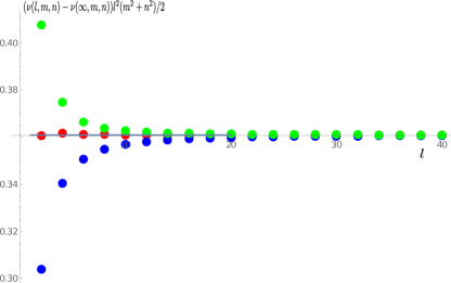
Figure 8: Convergence of the scaled difference $\left(\nu(l,m,n)-\nu(\infty,m,n)\right)l^{2}\left(m^{2}+n^{2}\right)/2$ to the limiting value $5\sqrt{3}/24\simeq 0.360844$ for $(m,n)=(0,1)$ – blue dots, $(m,n)=(1,1)$ – green dots and $(m,n)=(1,2)$ – red dots.

In the same way one can study the next finite size corrections, which though are not expected to be universal, still may contain a sort of universal amplitudes. An example was given in [16], where the quantity

$$l^{4}\left(\nu(l,1,1)-\nu(\infty,1,1)-\frac{5\sqrt{3}}{24}\frac{1}{l^{2}}\right)\simeq a+\frac{b}{l^{2}}$$ (41)

was studied. The coefficients were estimated to $a=0.180$ and $b=0.69$. Our estimate based on the fit of the scaled difference calculated for the circumferences up to $l=100$ shows

$$a=0.1804(2),b=0.47(6).$$ (42)

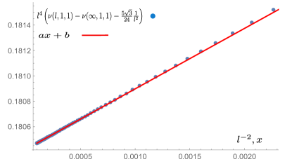
Figure 9: Comparison of the corrections to the densities (41) calculated at $20\leq l\leq 100$ with the linear fit with parameters $a=0.1804$ and $b=0.47.$

It is interesting to see how the finite size corrections depend on the angle. This behavior may shed light on irrelevant operators of the theory responsible for the breaking of conformal invariance by the lattice. We perform similar at ten values of $(n,m)$ and study the dependence of the coefficients

$$a(\alpha)=\lim_{l\to\infty}\left(\frac{l^{2}\left(m^{2}+n^{2}\right)}{2}\right)^{2}\left(\nu(l,m,n)-\nu(\infty,m,n)-\frac{5\sqrt{3}}{12l^{2}\left(m^{2}+n^{2}\right)}\right)$$

and

$$\!\!\!\!\!\!\!\!\!\!\!\!\!\!\!\!\!\!\!\!\!\!\!\!\!\!b(\alpha)=\lim_{l\to\infty}\left(\frac{l^{2}\left(m^{2}+n^{2}\right)}{2}\right)^{3}\left(\nu(l,m,n)-\nu(\infty,m,n)-\frac{5\sqrt{3}}{12l^{2}\left(m^{2}+n^{2}\right)}-\frac{4a(\alpha)}{l^{4}\left(m^{2}+n^{2}\right)^{2}}\right)$$

on the angle $\alpha=\arctan(m/n)$. The results are presented in figs. 10,11.

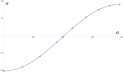
Figure 10: The values of scaled correction coefficient $a(\alpha)$ at ten values of the rotation angle $\alpha$ and its fit by $c_{1}+c_{2}\cos 4\alpha$ with $c_{1}=-0.0125,c_{2}=-0.192$.

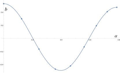
Figure 11: The values of scaled correction coefficient $b(\alpha)$ at ten values of the rotation angle $\alpha$ and its fit by $c_{3}+c_{4}\cos(4\alpha)+c_{5}\cos(8\alpha)$ with $c_{3}=0.00760,c_{4}=0.0273,c_{5}=0.495$.

They have clear periodic structure and are well fit with

$$a(\alpha) \simeq c_{1}+c_{2}\cos(4\alpha),$$

$$b(\alpha) \simeq c_{3}+c_{4}\cos(4\alpha)+c_{5}\cos(8\alpha),$$

with $c_{1}=-0.0125,c_{2}=-0.192$ and $c_{3}=0.00760,c_{4}=0.0273,c_{5}=0.495$. The quality of the fit can be tested on the exact values of expansion coefficients of $\nu(l,0,1)$ obtained from asymptotic expansion

$$\nu(l,0,1)=\left(\frac{3\sqrt{3}}{2}-\frac{5}{2}\right)+\frac{5}{8\sqrt{3}}\left(\frac{2}{l^{2}}\right)-\frac{205}{576\sqrt{3}}\left(\frac{2}{l^{2}}\right)^{2}+\frac{19025}{20736\sqrt{3}}\left(\frac{2}{l^{2}}\right)^{3}+O\left(\frac{1}{l^{8}}\right)$$ (43)

of the exact result in [1]. One can see that the the values of constants $c_{1},\dots,c_{5}$ obtained from the fits satisfy relations

$$a(0)=c_{1}+c_{2}=-0.2055\simeq-\frac{205}{576\sqrt{3}},$$ (44)

$$b(0)=c_{3}+c_{4}+c_{5}=0.5298\simeq\frac{19025}{20736\sqrt{3}}$$ (45)

with accuracy to three decimal places. The values of $a(\pi/4)=c_{1}-c_{2},b(\pi(4))=c_{3}-c_{4}+c_{5}$ reproduce (42) within the same accuracy. As explained in [56], the trigonometric functions of angles divisible by $4\alpha$ is a natural manifestation of breaking the rotational symmetry of the conformally invariant theory by the square lattice that results in appearance of operators whose conformal spin is multiple of four, see also [57, 58] for similar effects. It is interesting whether the values of constants $c_{1},\dots,c_{5}$ can be explained in the framework of CFT. This analysis can be considered as a preliminary step in systematic studies of the finite size corrections to cluster densities, and clearing up their conformal meaning.

For more detailed study of the finite size corrections one needs to perform the systematic asymptotic analysis of the solution of T-Q equation. This hopefully can be done with the non-linear integral equation technique developed in [59, 60] and applied in [45] to a proof of the conformal invariant form of the sub-leading finite size correction to free energy of the six-vertex model on the rotated lattice. Whether this technique is suitable for systematic analysis of the next to sub-leading corrections to the derivatives of the free energy at the stochastic point is the matter for further investigation.

Appendix A Exact densities

$m=1,n=2$

$l$	$\nu_{\mathrm{c}}(l,1,2)$
$2$	$\frac{457}{4346}$
$4$	$\frac{2156027742167}{21586801226362}$
$6$	$\frac{431777998328921413810430569}{4366789318056412396314592982}$
$8$	$\frac{786294430244725543429301774315042465275143236939999}{7980483750425370301607306038647768778325881306171354}$
$10$	$\frac{3063214625120684629220276976212585297353537811730106923006124169424851246746977611251}{31141354303881719194901531792574953430390711629201099942966304916168344436205188871378}$

$l$	$\nu_{\mathrm{nc}}(l,1,2)$
$2$	$\frac{63}{2173}$
$4$	$\frac{78131053098}{10793400613181}$
$6$	$\frac{7013973470238361101359808}{2183394659028206198157296491}$
$8$	$\frac{7205724473170424432979362883354946667863166859216}{3990241875212685150803653019323884389162940653085677}$
$10$	$\frac{89949785674341668790750642180399072760356918123516183594046343010414953902267663104}{77853385759704297987253829481437383575976779073002749857415762290420861090512972178445}$

$l$	$\nu(l,1,2)$
$2$	$\frac{11}{82}$
$4$	$\frac{275693}{2573782}$
$6$	$\frac{22090069080005}{216378176911486}$
$8$	$\frac{8846218291444135690643021}{88168581201012456573730414}$
$10$	$\frac{12385236427151367035550969161665589631653003}{124449443496736607229791988937036731786613090}$

$m=1,n=4$

$l$	$\nu_{\mathrm{c}}(l,1,4)$
$2$	$\frac{3417329}{34119046}$
$4$	$\frac{4131823530849759693213650061797}{41903044260219093187283072814910}$
$6$	$\frac{52354510386464168141080291945089720530592239055392948076663254479940653}{532536631210089043138388552997130780273523772549104271499136454928074734}$

$l$	$\nu_{\mathrm{nc}}(l,1,4)$
$2$	$\frac{143712}{17059523}$
$4$	$\frac{44386921318627731749339096064}{20951522130109546593641536407455}$
$6$	$\frac{52354510386464168141080291945089720530592239055392948076663254479940653}{532536631210089043138388552997130780273523772549104271499136454928074734}$

$l$	$\nu(l,1,4)$
$2$	$\frac{1007}{9274}$
$4$	$\frac{950775017326855}{9439509175366346}$
$6$	$\frac{45931697658977271960510394658373737}{462768523437381762199714804256505814}$

$m=3,n=4$

$l$	$\nu_{\mathrm{c}}(l,3,4)$
$2$	$\frac{387768065791915313}{3895953850182322426}$
$4$	$\frac{44195116406974440581081566067289510598931484194160698978934613738812968820065999}{448965092769002158674204818544686846143985958937884255868928657300610488746952074}$

$l$	$\nu_{\mathrm{nc}}(l,3,4)$
$2$	$\frac{11343951399731931}{1947976925091161213}$
$4$	$\frac{324703379991987605772074955808303082817396322520577832155520445581250214007026}{224482546384501079337102409272343423071992979468942127934464328650305244373476037}$

$l$	$\nu(l,3,4)$
$2$	$\frac{505753025}{4800491638}$
$4$	$\frac{1025205092866657199069018079406719010967}{10263935640757775218890055689049451622658}$

References

• [1] Povolotsky A 2021 Journal of Physics A: Mathematical and Theoretical 54 22LT01
• [2] G G 1999 Percolation (Springer, Berlin, Heidelberg)
• [3] Kesten H 1982 Percolation theory for mathematicians vol 194 (Springer)
• [4] BollobΓ‘s B and Riordan O 2006 Percolation (Cambridge University Press)
• [5] Sykes M and Essam J 1963 Physical Review Letters 10 3
• [6] Sykes MΒ F and Essam JΒ W 1964 Journal of Mathematical Physics 5 1117–1127
• [7] Baxter RΒ J 2016 Exactly solved models in statistical mechanics (Elsevier)
• [8] Temperley HΒ N and Lieb EΒ H 1971 Proceedings of the Royal Society of London. A. Mathematical and Physical Sciences 322 251–280
• [9] Baxter RΒ J, Temperley H and Ashley SΒ E 1978 Proceedings of the Royal Society of London. A. Mathematical and Physical Sciences 358 535–559
• [10] Smirnov S 2001 Comptes Rendus de l’AcadΓ©mie des Sciences-Series I-Mathematics 333 239–244
• [11] BlΓΆte HΒ W, Cardy JΒ L and Nightingale MΒ P 1986 Physical review letters 56 742
• [12] Alcaraz FΒ C, Barber MΒ N and Batchelor MΒ T 1988 Annals of Physics 182 280–343
• [13] Hamer C, Quispel G and Batchelor M 1987 Journal of Physics A: Mathematical and General 20 5677
• [14] Nienhuis B 1987 Phase transitions and critical phenomena 11 1–53
• [15] Ziff RΒ M, Finch SΒ R and Adamchik VΒ S 1997 Physical review letters 79 3447
• [16] Kleban P and Ziff R 1998 Physical Review B 57 R8075
• [17] Chang SΒ C and Shrock R 2004 Physical Review E 70 056130
• [18] Chang SΒ C and Shrock R 2021 Physical Review E 104 044107
• [19] Baxter RΒ J, Kelland SΒ B and Wu FΒ Y 1976 Journal of Physics A: Mathematical and General 9 397
• [20] Razumov AΒ V and Stroganov YΒ G 2001 Journal of Physics A: Mathematical and General 34 3185
• [21] Batchelor M, DeΒ Gier J and Nienhuis B 2001 Journal of Physics A: Mathematical and General 34 L265
• [22] Razumov AΒ V and Stroganov YΒ G 2004 Theoretical and mathematical physics 138 333–337
• [23] Razumov AΒ V and Stroganov YΒ G 2005 Theoretical and mathematical physics 142 237–243
• [24] DeΒ Gier J 2005 Discrete mathematics 298 365–388
• [25] DiΒ Francesco P and Zinn-Justin P 2004 arXiv preprint math-ph/0410061
• [26] DiΒ Francesco P and Zinn-Justin P 2005 Journal of Physics A: Mathematical and General 38 L815
• [27] Zinn-Justin P 2006 arXiv preprint math/0607183
• [28] DiΒ Francesco P, Zinn-Justin P and Zuber J 2006 Journal of Statistical Mechanics: Theory and Experiment 2006 P08011
• [29] DiΒ Francesco P and Zinn-Justin P 2007 Journal of Statistical Mechanics: Theory and Experiment 2007 P12009
• [30] Razumov A, Stroganov YΒ G and Zinn-Justin P 2007 Journal of Physics A: Mathematical and Theoretical 40 11827
• [31] Cantini L and Sportiello A 2011 Journal of Combinatorial Theory, Series A 118 1549–1574
• [32] deΒ Gier J, Batchelor M, Nienhuis B and Mitra S 2002 Journal of Mathematical Physics 43 4135–4146
• [33] Mitra S, Nienhuis B, deΒ Gier J and Batchelor MΒ T 2004 Journal of Statistical Mechanics: Theory and Experiment 2004 P09010
• [34] deΒ Gier J, Jacobsen J and Ponsaing A 2016 SciPost Physics 1 012
• [35] Mitra S and Nienhuis B 2004 Journal of Statistical Mechanics: Theory and Experiment 2004 P10006
• [36] Alcaraz FΒ C, Brankov J, Priezzhev V, Rittenberg V and Rogozhnikov A 2014 Physical Review E 90 052138
• [37] Fujimoto M 1994 Journal of Physics A: Mathematical and General 27 5101
• [38] Yung C and Batchelor MΒ T 1995 Nuclear Physics B 435 430–462
• [39] Pronko GΒ P and Stroganov YΒ G 1999 Journal of Physics A: Mathematical and General 32 2333
• [40] Bajnok Z, Granet E, Jacobsen JΒ L and Nepomechie RΒ I 2020 Journal of High Energy Physics 2020 1–27
• [41] Fridkin V, Stroganov Y and Zagier D 2000 Journal of Physics A: Mathematical and General 33 L121
• [42] Fridkin V, Stroganov Y and Zagier D 2001 Journal of Statistical Physics 102 781–794
• [43] Zinn-Justin P 2009 arXiv preprint arXiv:0901.0665
• [44] AA L and VB P 1990 Journal of statistical physics 60 307–321
• [45] Fujimoto M 1996 Journal of statistical physics 82 1519–1539
• [46] Lieb EΒ H 1967 Physical Review Letters 18 692
• [47] Lieb EΒ H 2004 Exact solution of the two-dimensional slater kdp model of a ferroelectric Condensed Matter Physics and Exactly Soluble Models (Springer) pp 457–459
• [48] Lieb EΒ H 1967 Physical Review 162 162
• [49] Lieb EΒ H 2004 Exact solution of the f model of an antiferroelectric Condensed Matter Physics and Exactly Soluble Models (Springer) pp 453–455
• [50] Yang CΒ N and Yang CΒ P 1966 Physical Review 150 321
• [51] Yang CΒ N and Yang CΒ P 1966 Physical Review 150 327
• [52] Duminil-Copin H, Kozlowski KΒ K, Krachun D, Manolescu I and Tikhonovskaia T 2022 Communications in Mathematical Physics 395 1383–1430
• [53] Faddeev L 1996 arXiv preprint hep-th/9605187
• [54] Motegi K 2013 Journal of Mathematical Physics 54 063510
• [55] Ziff R private communications
• [56] Cardy JΒ L 1988 Les Houches 40
• [57] Couvreur R, Jacobsen JΒ L and Vasseur R 2017 Journal of Physics A: Mathematical and Theoretical 50 474001
• [58] Tan X, Couvreur R, Deng Y and Jacobsen JΒ L 2019 Physical Review E 99 050103
• [59] Klumper A, Batchelor MΒ T and Pearce PΒ A 1991 Journal of Physics A: Mathematical and General 24 3111
• [60] Klumper A, Wehner T and Zittartz J 1993 Journal of Physics A: Mathematical and General 26 2815