Game Theoretic Models for Profit-Sharing in Multi-fleet Platoons

Abstract

Profit-sharing is needed within platoons in order for competing transportation companies to collaborate in forming platoons. In this paper, we propose distribution models of the profit designed for vehicles that are located at the same origin and are operated by competing transportation companies. The vehicles have default departure times, but can decide to depart at other times in order to benefit from platooning. We model the strategic interaction among vehicles with game theory and consider pure Nash equilibria as the solution concept. In a numerical evaluation we compare the outcomes of the games associated with different distribution models of the profit.

I INTRODUCTION

The transport sector emitted $24\%$ of the total $\text{CO}_{2}$ emissions due to fuel combustion in 2016 and $74\%$ of the emissions from the transport sector was emitted from road transportation [1].

Truck platooning has received attention for its ability to reduce fuel consumption of road transportation. This is demonstrated in numerical studies in [2], [3] and by field experiments in [4], [5], [6], where potential fuel savings of up to $10\%$ are reported. Truck platooning has other benefits than reduced fuel consumption, e.g., decreased workload and cost of drivers, improved safety by reducing the human factor and reduced traffic congestion. The interested reader is referred to [7] for a high-level introduction to truck platooning.

Platoon matching is here used to denote the process of grouping vehicles (out of a pre-defined set of vehicles with fixed routes) that will form platoons. A review on planning strategies for truck platooning, including platoon matching, is given in [8]. When vehicles are operated by the same transportation company, the company would seek platoon formations to maximize the total profit from platooning of all its vehicles. In contrast, when vehicles are operated by different competing transportation companies, each vehicle may instead seek its platoon formation individually to maximize its own profit from platooning.

Distributing the profit from platooning is crucial for competing transportation companies to collaborate in forming platoons. This is due to unbalance in the profit of vehicles within platoons. For example, the platoon leaders’ fuel saving is small in comparison to its followers’ fuel savings [5]. Therefore, a vehicle needs compensation in order to agree on being a leader and contributing to the profit of its followers. The distribution model affects vehicles’ individual profit given their decided platoon formations which in turn affects vehicles’ decisions of platoon formations.

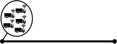
(a) Vehicles are located at the origin where they are communicating and deciding on their departure times.

(b) Vehicles with the same departure time are forming a platoon on the route between the origin and the destination.

Figure 1: Platooning scenario.

I-A Related work

Solutions to the platoon matching problem that aim to maximize the total profit from platooning of all vehicles have been proposed in the literature, e.g., [9], [10], [11], [12], [13].

Solutions to the platoon matching problem where vehicles individually seek to maximize their profits from platooning have been proposed in [14] and [15]. In these solutions, each vehicle seeks to minimize its traveling cost by deciding on its departure time from a common origin. The scenario is modeled as a non-cooperative game and Nash equilibrium is used as the solution concept. We study a similar scenario as in [14] and [15], but our focus is to propose different distribution models of the profit and study how they affect the total profit and the platoon rate.

The authors in [16] propose a solution to the platoon matching problem that aims to maximize the total profit of all vehicles. Then, the profit is distributed such that vehicles will have no incentive to leave their assigned platoons. Different to the work in [16], in this work, each vehicle seeks its platoon formation individually to maximize its own profit from platooning and the distribution model is known to the vehicles.

I-B Problem formulation

We consider vehicles located at a common origin and with a common destination. The origin could be, e.g., a ferry terminal, a freight consolidation center or a parking place. Each vehicle has a default departure time from the origin but can decide to depart at other times in order to benefit from platooning. Vehicles with the same departure time platoon with each other from the origin to the destination. The scenario is illustrated in Figure 1. The vehicles are operated by different competing transportation companies and each vehicle seeks its departure time in order to maximize its own profit. The profit is described by a utility function that includes the benefit of platooning and the cost of deviating from the default departure time. The strategic interaction among vehicles is modeled as a non-cooperative game and we use Nash equilibrium as solution concept.

The contributions of this work are:

1. Four conceptual models for distributing the platooning profit among the vehicles in the platoon, denoted even out, score system, market and cooperative.

2. A game formulation of the platoon matching problem based on the four models above and their solutions in terms of pure Nash equilibria.

3. A numerical study of how the four models are affecting the formation of platoons, the platooning rate, and the overall profit from platooning.

This paper is structured as follows. The platoon matching scenario that we consider is defined in Section II. Then, in Section III, the distribution models are proposed and a game associated with each distribution model is defined. In Section IV, the solution concepts for the platoon matching problems are defined and algorithms for finding the solutions are presented. The algorithms are then used when comparing the outcomes of the games associated with the distribution models in the numerical evaluation in Section V. Finally, conclusions and future work are given in Section VI.

II Platoon matching scenario

Consider the scenario in Figure 1. Vehicles start at a common location, called origin, and have a common destination. Each vehicle has its own default departure time from the origin but can decide to depart at another time in order to benefit from platooning. The vehicles are enumerated from $1$ to $N$ and we define the index set $\mathcal{N}=\{1,...,N\}$.

Vehicles’ decisions in the platoon matching scenario are their departure times. The departure times of vehicles are represented by integer-valued time-steps. The decided departure time of vehicle $i$ is $d_{i}\in\mathbb{Z}_{+}$. The set of departure times of the vehicles in $\mathcal{N}$ is denoted $\mathbf{d}=\{d_{i}|i\in\mathcal{N}\}$. The default departure time of vehicle $i$ is denoted $d_{i}^{\star}$ and the set of default departure times is denoted $\mathbf{d}^{\star}$. The set of departure times of all vehicles except vehicle $i$ is denoted $\mathbf{d}_{-i}=\mathbf{d}\setminus\{d_{i}\}$.

A vehicle can only depart at one of the default departure times in $\mathbf{d}^{\star}$ and each vehicle $i$ is constrained to not depart earlier than $d_{i}^{\star}$ and not later than $d_{i}^{\star}+\delta_{i}$, where $\delta_{i}$ is the maximum delay of vehicle $i$. The set of possible departure times of vehicle $i$ is $\mathcal{D}_{i}=\{t\in\mathbf{d}|d_{i}^{\star}\leq t\leq d_{i}^{\star}+\delta_{i}\}$. The space of possible departure times of the vehicles in $\mathcal{N}$ is $\mathcal{D}=\{\boldsymbol{d}|d_{i}\in\mathcal{D}_{i},\forall i\in\mathcal{N}\}$.

If two or more vehicles decide on the same departure time they will form a platoon. The index set of vehicles in the platoon that leaves at time $d_{i}^{\star}$ is

$$\mathcal{N}_{i}(\mathbf{d})=\{k\in\mathcal{N}|d_{k}=d_{i}^{\star}\}$$

and the number of vehicles in the platoon is the cardinality of the index set, denoted $|\mathcal{N}_{i}(\mathbf{d})|$. Note that $\mathcal{N}_{i}(\mathbf{d})$ will be empty for some $i$ when platoons are formed.

The profit from platooning differs for a platoon leader and its followers. Moreover, we allow the profit to be vehicle dependent. The profit of vehicle $i$ is $R_{i}^{l}$ when it is a platoon leader between the origin and the destination. The profit of vehicle $i$ is $R_{i}^{f}$ when it is a platoon follower between the origin and destination. Typically, $R_{i}^{l}<R_{i}^{f}$.

There is a cost associated with departing later than the default time, e.g., due to increased driver cost and cost related to later arrival of goods. If vehicle $i$ departs at $d_{i}$ its time-penalty is $B_{i}(d_{i})$. We assume that, $B_{i}(d_{i}^{\star})=0$ and $B_{i}(d_{i})\geq 0$.

III Distribution models of the profit from platooning

In this section we propose four models describing how the profit from platooning is distributed among vehicles. Each distribution model results in a model of vehicles’ utility functions. Since a vehicle’s profit changes whether it is a leader or a follower, a mechanism for assigning the leaders associated to each distribution model is proposed.

III-A Distribution model 1: even out

In this model, the leader of the platoon receives a monetary compensation from its followers, according to a standardized agreement, to even out unbalance in the profit between the leader and its followers. Moreover, the platoon leader is assigned randomly.

Vehicles do not have to reveal the actual individual profit from platooning; this might be information that they want to keep secret. However, they have agreed on standard values of the profit from platooning between the origin and the destination. The standard values of the profit for being a leader and follower are denoted $R^{l}$ and $R^{f}$ respectively. In a platoon of $n>1$ members, the transaction from each follower to the leader is $\frac{1}{n}(R^{f}-R^{l})$. If vehicle $i$ is a leader in a platoon of $n$ vehicles, its profit from platooning after the transaction is,

$$R_{i}^{l}+\frac{n-1}{n}(R^{f}-R^{l})$$ (1)

and if vehicle $i$ is a follower its profit is

$$R_{i}^{f}-\frac{1}{n}(R^{f}-R^{l}).$$ (2)

Remark 1.

If $R^{f}=R_{1}^{f}=...=R_{N}^{f}$ and $R^{l}=R_{1}^{l}=...=R_{N}^{l}$, the profit of a leader equals the profit of its followers after the transaction. That is, (1) equals (2).

The leader in each platoon is randomly drawn from the platoon members with equal probability. In a platoon of $n$ members, the probability of each vehicle to be drawn to be a follower or the leader are $\frac{n-1}{n}$ and $\frac{1}{n}$, respectively. Then, if vehicle $i$ is in a platoon of length $n>1$, the expected profit of vehicle $i$ is

$$\frac{1}{n}\left(R_{i}^{l}+\frac{n-1}{n}(R^{f}-R^{l})\right)+\frac{n-1}{n}\left(R_{i}^{f}-\frac{1}{n}(R^{f}-R^{l})\right)$$

which equals

$$\frac{1}{n}R_{i}^{l}+\frac{n-1}{n}R_{i}^{f}.$$

Remark 2.

Given the random leader assignment, the expected profit from platooning after the transaction is independent of the standard profits $R_{l}$ and $R_{f}$.

Utility function 1 (even out).

For each vehicle $i\in\mathcal{N}$ and given departure times $d_{i}=d_{j}^{\star}$ and $\boldsymbol{d}_{-i}$, if vehicle $i$ departs in a platoon with other vehicles, i.e., $|\mathcal{N}_{j}(d_{i},\boldsymbol{d}_{-i})|>1$, then the utility function of vehicle $i$ is defined as

$$u_{i}^{eo}(d_{i},\boldsymbol{d}_{-i})=\!\frac{1}{|\mathcal{N}_{j}(d_{i},\boldsymbol{d}_{-i})|}R_{i}^{l}+\frac{|\mathcal{N}_{j}(d_{i},\boldsymbol{d}_{-i})|-1}{|\mathcal{N}_{j}(d_{i},\boldsymbol{d}_{-i})|}R_{i}^{f}\!-\!B_{i}(d_{i}),$$

where the two first terms are the expected profit of platooning and the third term is the time-penalty. If vehicle $i$ departs alone, i.e., $|\mathcal{N}_{j}(d_{i},\boldsymbol{d}_{-i})|=1$, then $u_{i}^{eo}(d_{i},\boldsymbol{d}_{-i})=-B_{i}(d_{i})$.

III-B Distribution model 2: score system

Vehicles have scores that increase every time they are platoon leaders and decrease every time they are platoon followers. In each platoon formation, the vehicle with the lowest score becomes the leader. The idea is that the profit from platooning is balanced over time by the score system.

The score of vehicle $i$ is denoted $s_{i}$ and the set of scores of the vehicles in $\mathcal{N}$ is $\boldsymbol{s}=\{s_{i}|i\in\mathcal{N}\}$. It is assumed that each vehicle has a unique score. If vehicle $i$ departs with other vehicles, i.e., $|\mathcal{N}_{j}(d_{i},\boldsymbol{d}_{-i})|>1$ and it has the lowest score in the platoon, i.e., $s_{i}<s_{j}$ for all $j\in\mathcal{N}_{j}(d_{i},\boldsymbol{d}_{-i})$, then vehicle $i$ becomes the leader. Otherwise it becomes a follower.

The scores of vehicles are updated as follows. If vehicle $i$ has score $s_{i}$ and becomes the leader of the platoon of vehicles in $\mathcal{N}_{j}(d_{i},\boldsymbol{d}_{-i})$, its score next time it platoons is

$$s_{i}+\Delta s^{l}\left(\mathcal{N}_{j}(d_{i},\boldsymbol{d}_{-i})\right)$$

and if vehicle $i$ becomes a platoon follower its score next time it platoons is

$$s_{i}-\Delta s^{f}\left(\mathcal{N}_{j}(d_{i},\boldsymbol{d}_{-i})\right)$$

and if vehicle $i$ departs alone its score next time it platoons is $s_{i}$. Vehicle $i$ valuates each unit of score as $\beta_{i}$.

Utility function 2 (score system).

Given departure times $d_{i}=d_{j}^{\star}$ and $\boldsymbol{d}_{-i}$, and given the scores $\boldsymbol{s}$, if vehicle $i$ departs in a platoon with other vehicles, i.e., $|\mathcal{N}_{j}(d_{i},\boldsymbol{d}_{-i})|>1$, and it becomes the leader according to the score system, then its utility is

$$u_{i}^{s}(d_{i},\boldsymbol{d}_{-i},\boldsymbol{s})=R_{i}^{l}-B_{i}(d_{i})+\beta_{i}\Delta s^{l}(\mathcal{N}_{j}(d_{i},\boldsymbol{d}_{-i})),$$

where the first term is its profit from platooning, the second term is the time-penalty and the third term is its valuation of the score update. If vehicle $i$ becomes a follower according to the score system its utility is

$$u_{i}^{s}(d_{i},\boldsymbol{d}_{-i},\boldsymbol{s})=R_{i}^{f}-B_{i}(d_{i})-\beta_{i}\Delta s^{f}(\mathcal{N}_{j}(d_{i},\boldsymbol{d}_{-i})).$$

If vehicle $i$ departs alone, i.e., $|\mathcal{N}_{j}(d_{i},\boldsymbol{d}_{-i}))|=1$, then its utility is $u_{i}^{s}(d_{i},\boldsymbol{d}_{-i},\boldsymbol{s})=-B_{i}(d_{i})$.

III-C Distribution model 3: market

A sub-set of the vehicles are sellers and the rest of the vehicles are buyers. Each seller offers the buyers to be platoon followers for a price that the seller decides. The buyers decide which seller to follow. Then, each seller seeks the price that maximizes its own profit which is a combination of its profit for being a leader and the payment it receives from the followers.

The sellers are in the set $\mathcal{N}_{s}\subseteq\mathcal{N}$ and the buyers are in the set $\mathcal{N}_{b}=\mathcal{N}\setminus\mathcal{N}_{s}$. The sellers always depart at their default departure times, more precisely, $d_{i}=d_{i}^{\star}$ for $i\in\mathcal{N}_{s}$. Moreover, sellers have unique departure times, that is, $d^{\star}_{i}\neq d_{j}^{\star}\ \forall i,j\in\mathcal{N}_{s}$ when $i\neq j$. The departure times of all sellers are in the set $\mathcal{D}_{s}=\{d_{i}^{\star}|i\in\mathcal{N}_{s}\}$.

The price of seller $i$ is denoted $p_{i}$. The set of prices of the sellers in $\mathcal{N}_{s}$ is denoted $\boldsymbol{p}=\{p_{i}|i\in\mathcal{N}_{s}\}$. The set of prices of the sellers in $\mathcal{N}_{s}$ except for seller $i$ is denoted $\boldsymbol{p}_{-i}=\boldsymbol{p}\setminus\{p_{i}\}$. The price of seller $i$ takes values in the finite set $\mathcal{P}_{i}$. The space of prices of the sellers in $\mathcal{N}_{s}$ is $\mathcal{P}=\{\boldsymbol{p}|p_{i}\in\mathcal{P}_{i},\ \forall i\in\mathcal{N}_{s}\}$.

Given the prices of sellers, each buyer is assumed to follow the seller that maximizes its profit, or to depart alone at its own default departure time if that is more profitable. Then, buyer $j$ decides one of the departure times in the set $\mathcal{D}_{j}^{*}=(\mathcal{D}_{s}\cap\mathcal{D}_{j})\cup\{d_{j}^{\star}\}$. If buyer $j$ departs at the default departure time of seller $i$ its profit is $R_{j}^{f}-p_{i}-B_{j}(d_{i}^{\star})$ and if buyer $j$ departs alone at its own default departure time its profit is zero which can be written as $R_{j}^{f}-p_{j}-B_{j}(d_{j}^{\star})$, where we define $p_{j}=R_{j}^{f}$ and have $B_{j}(d_{j}^{\star})=0$. Then, the most profitable departure time of buyer $j$, given the prices $\boldsymbol{p}$, is

$$d_{j}(\boldsymbol{p})=\underset{d_{i}^{\star}\in\mathcal{D}_{j}^{*}}{\text{argmax}}\ R_{j}^{f}-p_{i}-B_{j}(d_{i}^{\star}).$$ (3)

In addition, the index set of buyers that follow seller $i$ is $F_{i}(p_{i},\boldsymbol{p}_{-i})=\{j\in\mathcal{N}_{b}|d_{j}(p_{i},\boldsymbol{p}_{-i})=d_{i}^{\star}\}$.

Remark 3.

The buyers depart according to (3) and the profit of buyers are solely dependent on the prices of the sellers.

Utility function 3 (market).

For each seller $i\in\mathcal{N}_{s}$ and given prices $p_{i}$ and $\boldsymbol{p}_{-i}$, if seller $i$ is a leader for at least one buyer, i.e. $|F_{i}(p_{i},\boldsymbol{p}_{-i})|>0$, then the utility function of vehicle $i$ is

$$u_{i}^{m}(p_{i},\boldsymbol{p}_{-i})=R_{i}^{l}+|F_{i}(p_{i},\boldsymbol{p}_{-i})|p_{i}$$

where the first term is the profit for being a leader and the second term is the received payment from the followers. If vehicle $i$ departs without followers, i.e., $|F_{i}(p_{i},\boldsymbol{p}_{-i})|=0$, then, $u_{i}^{m}(p_{i},\boldsymbol{p}_{-i})=0$.

Remark 4.

The set of sellers $\mathcal{N}_{s}$ is in many cases not given. In Section IV an algorithm will be proposed that assigns the set of sellers.

III-D Distribution model 4: cooperative

The distribution models even out, score system and market are suitable when the vehicles are operated by different competing transportation companies. A distribution model that is suitable when the vehicles are operated by the same transportation company is proposed in this sub-section. The transportation company seeks departure times of its vehicles to maximize the total profit from platooning and minimize the total time-penalty of its vehicles.

In each platoon, the leader is assigned to maximize the total profit. That is, in each platoon, the vehicle with the smallest difference in profit for being a platoon follower and platoon leader is assigned to be the platoon leader. The profit from platooning connected to vehicle $i$ is $b_{i}(\boldsymbol{d})=R_{i}^{f}$ if it is a follower and $b_{i}(\boldsymbol{d})=R_{i}^{l}$ if it is a leader. The profit connected to vehicle $i$ if it departs alone is $b_{i}(\boldsymbol{d})=0$.

Utility function 4 (cooperative).

Given departure times $\boldsymbol{d}$, the common utility function of the vehicles in $\mathcal{N}$ is

$$u^{c}(\boldsymbol{d})=\sum\limits_{j\in\mathcal{N}}\big{(}b_{j}(\boldsymbol{d})-B_{j}(d_{j})\big{)},$$

which is the sum of the profit of the vehicles and their time-penalties.

III-E Spontaneous platooning

In this model, the vehicles depart at their default departure times, i.e., $\boldsymbol{d}=\boldsymbol{d}^{\star}$. Thus, the vehicles do not have any decision to make. Vehicles that have the same default departure time platoon spontaneously. The individual utility of vehicle $i$ is $u_{i}^{eo}(d_{i}^{\star},\boldsymbol{d}_{-i}^{\star})$, which is the utility function of the distribution model even out when vehicles depart at their default departure times.

IV Platoon matching games and their solutions

A game associated with each distribution model is defined in Section IV-A. The games are used to model the rational behavior of the decision-makers, and their solution decisions correspond to pure Nash equilibria of the games. The pure Nash equilibrium is defined, and an algorithm that seeks for it is proposed in Section IV-B. In the same section, an algorithm is proposed for assigning the sellers of the game associated with the distribution model market.

IV-A Defining the games

The distribution models even out and score system result in non-cooperative games where the players are the vehicles and the decisions, decision space and utility functions are defined in Section III. The game associated with the distribution model even out is $G^{eo}=(\mathcal{N},\mathcal{D},\mathcal{U}^{eo}(\boldsymbol{d}))$ where $\mathcal{U}^{eo}(\boldsymbol{d})=\{u_{i}^{eo}(d_{i},\boldsymbol{d}_{-i})|i\in\mathcal{N}\}$. The game associated with the distribution model score system is $G^{s}=(\mathcal{N},\mathcal{D},\mathcal{U}^{s}(\boldsymbol{d},\boldsymbol{s}))$ where $\mathcal{U}^{s}(\boldsymbol{d},\boldsymbol{s})=\{u_{i}^{s}(d_{i},\boldsymbol{d}_{-i},\boldsymbol{s})|i\in\mathcal{N}\}$.

The distribution model market results in a non-cooperative game where the players are the sellers and decisions variables are their prices. The associated game is $G^{m}=(\mathcal{N}_{s},\mathcal{P},\mathcal{U}^{m}(\boldsymbol{p}))$, where $\mathcal{U}^{m}(\boldsymbol{p})=\{u_{i}^{m}(p_{i},\boldsymbol{p}_{-i})|i\in\mathcal{N}_{s}\}$.

The distribution model cooperative represents a case where all vehicles are interested in maximizing a common utility function $u^{c}(\boldsymbol{d})$. It is hard to find a global maximizer to the platoon matching problem due to its combinatorial structure. Instead we seek for sub-optimal solutions by letting each vehicle $i$ seek for its departure time $d_{i}$ that maximizes $u^{c}(d_{i},\boldsymbol{d}_{-i})$. Then, the interaction among vehicles is modeled by the cooperative game $G^{c}=(\mathcal{N},\mathcal{D},u^{c}(\boldsymbol{d}))$ and we define $u_{i}^{c}(d_{i},\boldsymbol{d}_{-i})=u^{c}(d_{i},\boldsymbol{d}_{-i})$.

IV-B Solutions of the games

First, for each of the games $G^{eo}$, $G^{s}$ and $G^{c}$, and given the decisions $d_{i}$ and $\boldsymbol{d}_{-i}$, let $u_{i}(d_{i},\boldsymbol{d}_{-i})$ temporarily denote the individual utility function of vehicle $i$. A pure Nash equilibrium is a decision profile $\boldsymbol{d}^{*}\in\mathcal{D}$ such that

$$u_{i}(d_{i}^{*},\boldsymbol{d}_{-i}^{*})\geq u_{i}(d_{i},\boldsymbol{d}_{-i}^{*}),\ \forall d_{i}\in\mathcal{D}_{i},\ \forall i\in\mathcal{N}.$$ (4)

The best-response function of vehicle $i$ given $\boldsymbol{d}_{-i}$ is defined as

$$B_{i}(\boldsymbol{d}_{-i})=\underset{d_{i}\in\mathcal{D}_{i}}{\arg\max}\ u_{i}(d_{i},\boldsymbol{d}_{-i}).$$ (5)

Remark 5.

In (4) and (5), pure Nash equilibria and the best-response function were defined for the games $G^{eo}$, $G^{s}$ and $G^{c}$. However, pure Nash equilibria and the best-response function can be defined similarly for the game $G^{m}$. Pure Nash equilibria of the game $G^{m}$ are denoted $\boldsymbol{p}^{*}$ and the best-response function of seller $i$ given the prices $\boldsymbol{p}_{-i}$ is denoted $B_{i}(\boldsymbol{p}_{-i})$.

Algorithm 1 seeks for pure Nash equilibria by letting each vehicle, one at a time, update its decision according to its best-response function. The limiting decision profile is a pure Nash equilibrium and it is used later in the numerical evaluation as the solution of the games.

Algorithm 2 assigns sellers of the game $G^{m}$ and seeks for its pure Nash equilibria. The approach is to first find an equilibrium (using Algorithm 1) of an initial set of sellers, possibly all vehicles. Then, one of the sellers that departs without followers becomes a buyer. Then, an equilibrium is found considering the reduced set of sellers. This procedure is repeated until all sellers depart with followers. The limiting set of sellers $\mathcal{N}_{s}^{*}$ is used as the set of the assigned sellers in the numerical evaluation and the solution of corresponding game is the limiting pure Nash equilibrium.

input : Initial decisions, $\boldsymbol{d}=(d_{1},...,d_{N})$

output : Pure Nash equilibrium, $\boldsymbol{d}^{*}=(d_{1}^{*},...,d_{N}^{*})$

$\boldsymbol{d}^{old}\neq\boldsymbol{d}$

while $\boldsymbol{d}^{old}\neq\boldsymbol{d}$  do

       $\boldsymbol{d}^{old}=\boldsymbol{d}$

       for $i\in\mathcal{N}$ do

             $d_{i}=B_{i}(\boldsymbol{d}_{-i})$

       end for

      

end while

$\boldsymbol{d}^{*}=\boldsymbol{d}$

Algorithm 1 Seeks for pure Nash equilibria.

input : Initial sellers, $\mathcal{N}_{s}=\mathcal{N}$

Initial buyers, $\mathcal{N}_{b}=\emptyset$

Initial prices, $\boldsymbol{p}$

output : Assigned sellers, $\mathcal{N}_{s}^{*}$

Pure Nash equilibrium, $\boldsymbol{p}^{*}$

$\mathcal{A}=\mathcal{N}$

while $\mathcal{A}\neq\emptyset$  do

      

      $\boldsymbol{p}^{old}\neq\boldsymbol{p}$

      

      while $\boldsymbol{p}^{old}\neq\boldsymbol{p}$  do

             $\boldsymbol{p}^{old}=\boldsymbol{p}$

             for $i\in\mathcal{N}_{s}$ do

                   $p_{i}=B_{i}(\boldsymbol{p}_{-i})$

             end for

            

       end while

      

      $A=\{i\in\mathcal{N}_{s}||F_{i}|=0\}$

      if $\mathcal{A}\neq\emptyset$ then

             Pick one seller $i\in A$

             $\mathcal{N}_{s}=\mathcal{N}_{s}\cap\{i\}$

             $\mathcal{N}_{b}=\mathcal{N}_{b}\cup\{i\}$

             $\boldsymbol{p}=\boldsymbol{p}_{-i}$

       end if

      

end while

$\mathcal{N}_{s}^{*}=\mathcal{N}_{s}$

$\boldsymbol{p}^{*}=\boldsymbol{p}$

Algorithm 2 Select sellers and seeks for pure Nash equilibria of the game $G^{m}$.

V Numerical evaluation

The proposed algorithms in Section IV are used here to find solutions of the platoon matching games. The games model the interaction among vehicles when different models of profit distribution are used. First, the set-up of the numerical evaluation is presented. Second, the outcomes of the platoon matching games are compared.

V-A Set-up of simulation

The considered scenario is illustrated in Figure 1 and defined in Section II. The distance between the origin and destination is $200$ kilometers. The benefit from platooning is, in this simulation, considered to be the reduction of fuel consumption. We assume the percentage of fuel savings of the platoon followers and leaders to be $10\%$ and $0\%$, respectively. Moreover, we assume that each vehicle consumes $0.35$ liters of fuel per kilometer and the fuel price is $15$ SEK (Swedish Krona) per liter. Then, the profit of the followers and leaders are $R_{1}^{f}=...=R_{N}^{f}=105$ SEK and $R_{1}^{l}=...=R_{N}^{l}=0$, respectively.

Vehicles’ default departure times from the origin are all within a $30$ minutes interval. The default departure time of each vehicle $i$ is drawn from the set $\{0,1,...,30\}$ and each outcome has equal probability, i.e., $d_{i}^{\star}\sim\mathcal{U}\{0,30\}.$ The maximum time delay of vehicle $i$ is $\delta_{i}=10$ minutes, i.e., its possible departure times are in the set $\mathcal{D}_{i}=\{d_{i}^{\star},d_{i}^{\star}+1,...,d_{i}^{\star}+10\}$.

The vehicles are penalized with $10$ SEK for each minute they deviate from their default departure time. The time-penalty for each vehicle $i$ is $B_{i}(d_{i})=10(d_{i}-d_{i}^{\star})$.

In the distribution model score system, in this set-up, it is assumed that the score update of the leader in a platoon equals the sum of the score updates of its followers. Then, for the platoon of the vehicles in $\mathcal{N}_{j}(\boldsymbol{d})$ the score update of the leader is $\Delta s^{l}(\mathcal{N}_{j}(\boldsymbol{d}))=\frac{|\mathcal{N}_{j}(\boldsymbol{d})|-1}{|\mathcal{N}_{j}(\boldsymbol{d})|}$ and the score update of the followers is $\Delta s^{f}(\mathcal{N}_{j}(\boldsymbol{d}))=-\frac{1}{|\mathcal{N}_{j}(\boldsymbol{d})|}$. Moreover, the vehicles valuate each score unit as $\beta_{i}=\frac{R^{f}}{4}$.

In the distribution model market, in this set-up, each seller decides on its price from the set $\mathcal{P}_{i}=\{\frac{1}{5}105,\frac{2}{5}105,\frac{3}{5}105,\frac{4}{5}105\}$. Note that it is not reasonable for a seller to decide a price higher or equal to $105$ SEK since then the price exceeds the profit of platooning of the buyers and the seller will then get zero followers.

V-B Comparison of different distribution models

The outcomes of the games associated with the distribution models even out, score system, market, cooperative and the spontaneous platooning presented in Section III-E, are compared. The number of vehicles $N$ is varied from $1$ to $29$ in the numerical evaluation and we keep the interval of the default departure times fixed at $30$ minutes. Monte Carlo simulations are used to approximate the expected outcome of the games. The simulation was carried out $50$ times for each game and number of vehicles $N$.

The average individual utility of the distribution models is shown in Figure 2(a). We see that the highest individual utility is obtained for the cooperative distribution model. This is expected since the vehicles aim to maximize the total utility of all vehicles. Close to the utility of cooperative distribution is the utility of even out and the utility of score system is lower than the utility of the even out. This can be explained by the fact that vehicles with low score have low incentive to deviate from their default departure time and platooning opportunities are not exploited. The utility of market is low in comparison to the other distribution models. This is explained by the fact that buyers tend to spread out on sellers even when their default departure times are close which obtains lower total utility than if they depart in the same platoon. The spontaneous solution obtained lowest utility, as expected.

The percentage of followers is shown in Figure 2(b). We see that when the number of vehicles is greater than $8$, the percentage of followers is higher in the solutions of score system than in cooperative and even out, even though the average utility is higher for cooperative and even out. This is possible because a higher percentage of platoon followers implies fewer platoons which can lead to higher total time-penalty and therefore lower utility.

VI Conclusions and future work

Models for distributing the profit from platooning have been proposed and the interaction among vehicles for each distribution model was modeled as a game. In a numerical evaluation it was seen that the highest individual utility was obtained when all vehicles shared both the profit from platooning and the time-penalty (cooperative). Moreover, it was seen that the individual utility was almost as high when the leaders received profit from its followers to even out the profit (even out). This suggests that, if the profit is shared in a fair way, competing companies can obtain a total profit from platooning that is near the cooperative solution, by acting selfishly. Moreover, it was seen that the spontaneous solution obtained a low utility and low platoon rate, which suggests that active platoon matching is important to increase vehicles’ profit from platooning.

In future work we will extend the distribution models to be suitable for cases where the vehicles have different origins and destinations. Additionally, in our models we will capture that vehicles’ profits depend on the ordering of vehicles in the platoons and design suitable profit-sharing models.

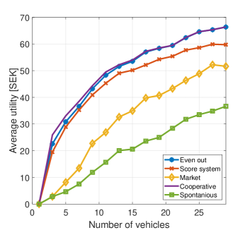
(a) Average individual utility.

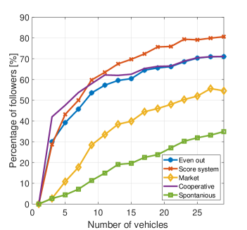
(b) Percentage of followers.

Figure 2: Comparison of distribution models.

References

- [1] OECD, CO2 Emissions from Fuel Combustion 2018. Paris: Organization for Economic Cooperation and Development, 2018.
- [2] A. Davila, E. del Pozo, E. Aramburu, and A. Freixas, “Environmental benefits of vehicle platooning,” in Symposium on International Automotive Technology 2013, jan 2013.
- [3] R. Bishop, D. Bevly, L. Humphreys, S. Boyd, and D. Murray, “Evaluation and testing of driver-assistive truck platooning phase 2 final results,” Transportation Research Record, vol. 2615, no. 2615, pp. 11–18, 2017.
- [4] A. Alam, A. Gattami, and K. H. Johansson, “An experimental study on the fuel reduction potential of heavy duty vehicle platooning,” in 13th International IEEE Conference on Intelligent Transportation Systems, pp. 306–311, Sept 2010.
- [5] F. Browand, J. McArthur, and C. Radovich, “Fuel saving achieved in the field test of two tandem trucks,” Technical report, University of Sourthern California, 2004.
- [6] S. Tsugawa, S. Jeschke, and S. E. Shladover, “A review of truck platooning projects for energy savings,” IEEE Transactions on Intelligent Vehicles, vol. 1, pp. 68–77, March 2016.
- [7] A. Alam, B. Besselink, V. Turri, J. Mårtensson, and K. H. Johansson, “Heavy-duty vehicle platooning for sustainable freight transportation: A cooperative method to enhance safety and efficiency,” IEEE Control Systems Magazine, vol. 35, pp. 34–56, Dec 2015.
- [8] A. K. Bhoopalam, N. Agatz, and R. Zuidwijk, “Planning of truck platoons: A literature review and directions for future research,” Transportation Research Part B, vol. 107, pp. 212–228, 2018.
- [9] K. Liang, J. Mårtensson, and K. H. Johansson, “Heavy-duty vehicle platoon formation for fuel efficiency,” IEEE Transactions on Intelligent Transportation Systems, vol. 17, pp. 1051–1061, April 2016.
- [10] E. Larsson, G. Sennton, and J. Larson, “The vehicle platooning problem: Computational complexity and heuristics,” Transportation Research Part C: Emerging Technologies, vol. 60, pp. 258 – 277, 2015.
- [11] S. van de Hoef, K. H. Johansson, and D. V. Dimarogonas, “Fuel-efficient en route formation of truck platoons,” IEEE Transactions on Intelligent Transportation Systems, vol. 19, pp. 102–112, Jan 2018.
- [12] N. Boysen, D. Briskorn, and S. Schwerdfeger, “The identical-path truck platooning problem,” Transportation Research Part B: Methodological, vol. 109, pp. 26 – 39, 2018.
- [13] R. Larsen, J. Rich, and T. kjær Rasmussen, “Hub-based truck platooning: Potentials and profitability,” Transportation Research Part E: Logistics and Transportation Review, vol. 127, pp. 249 – 264, 2019.
- [14] F. Farokhi and K. H. Johansson, “A game-theoretic framework for studying truck platooning incentives,” in 16th International IEEE Conference on Intelligent Transportation Systems (ITSC 2013), pp. 1253–1260, Oct 2013.
- [15] A. Johansson, E. Nekouei, K. H. Johansson, and J. Mårtensson, “Multi-fleet platoon matching: A game-theoretic approach,” in 2018 21st International Conference on Intelligent Transportation Systems (ITSC), pp. 2980–2985, Nov 2018.
- [16] X. Sun and Y. Yin, “Behaviorally stable vehicle platooning for energy savings,” Transportation Research Part C: Emerging Technologies, vol. 99, pp. 37 – 52, 2019.