Analytic solutions and numerical method

for a coupled thermo-neutronic problem

François Dubois^abc and Olivier Lafitte^ad

^a International Research Laboratory 3457 du Centre National de la Recherche Scientifique,

Centre de Recherches Mathématiques, Université de Montréal, Montréal, QC, Canada.

^b Conservatoire National des Arts et Métiers, LMSSC laboratory, Paris, France.

^c Laboratoire de Mathématiques d’Orsay, Université Paris-Saclay, France.

^d Université Paris 13, Sorbonne Paris Cité, LAGA, CNRS (UMR 7539),

99 Avenue J.-B. Clément F-93430, Villetaneuse Cedex, France.

10 May 2022

Keywords: ordinary differential equation, analytic functions, thermohydraulics, neutronics, Crank-Nicolson numerical scheme.

Abstract

We consider in this contribution a simplified idealized one-dimensional coupled model for neutronics and thermo-hydraulics under the low Mach number approximation. We propose a numerical method treating globally the coupled problem for finding its unique solution. Simultaneously, we use incomplete elliptic integrals to represent analytically the neutron flux. Both methods match perfectly. Note that the multiplication factor, classical output of neutronics problems, depends considerably of the representation of the cross sections.

1. Introduction

In this note, we recall briefly the construction of an analytic solution of the low Mach number thermohydraulic model obtained by Dellacherie et al. detailed in [7]. Assuming that the neutronics problem, stated in a 1d setting as

(1) $$\left\{\begin{array}[]{l}\frac{d}{dz}(D(h(z))\frac{d\phi}{dz})+\Sigma_{a}(h(z))\phi(z)=\frac{\nu\Sigma_{f}(h(z))}{k_{eff}}\phi(z),\\ \qquad\qquad z\in[0,L],\phi(0)=\phi(z)=0,\phi\geq 0\end{array}\right.$$

where $\phi$ is the neutron density, $h$ is the enthalpy (a measure of the temperature), $\Sigma_{a}$ and $\nu\Sigma_{f}$ are respectively the absorption and fission cross section of the fissile material, $D$ is the diffusion coefficient. This equation is coupled with an equation on the enthalpy:

(2) $$h^{\prime}(z)=K\nu\Sigma_{f}(h)\phi(z)$$

supplemented with the boundary conditions $h(0)=h_{e}$, $h(L)=h_{s}$.

Recall that in [7], we constructed an analytical solution of (1) and (2) for any set of continuous positive functions $D,\Sigma_{a},\nu\Sigma_{f}$, as a generalisation of Dellacherie and Lafitte [6]. Indeed, introducing the two functions $\mathcal{X}$ and $\mathcal{Y}$ such that

$$\left\{\begin{array}[]{l}-\frac{d}{dh}(D(h)\nu\Sigma_{f}(h)\frac{d{\mathcal{X}}}{dh})=\frac{\Sigma_{a}(h)}{\nu\Sigma_{f}(h)},\\ -\frac{d}{dh}(D(h)\nu\Sigma_{f}(h)\frac{d{\mathcal{Y}}}{dh})=1,\quad\mathcal{X}(h_{e})=\mathcal{X}(h_{s})=\mathcal{Y}(h_{e})=\mathcal{Y}(h_{s})=0,\end{array}\right.$$

and defining $\Psi(h,k_{eff})=2(\frac{\mathcal{Y}(h)}{k_{eff}}-\mathcal{X}(h))$ we have shown that the problem of finding $k_{eff}$ resumes at using the unique solution $z\rightarrow h(z,k_{eff})$, increasing on $[0,L]$, such that $h(0,k_{eff})=h_{e}$, of

$$(h^{\prime}(z,k_{eff}))^{2}=\Psi(h(z,k_{eff}),k_{eff})$$

and at imposing $h(L,k_{eff})=h_{s}$, which is the equation on $k_{eff}$ to be solved. It has been proven in [6], [7] that

Lemma 1.1.

The equation

$$h(L,k_{eff})=h_{s}$$

has a unique solution $k_{eff}^{*}\in(0,(\mbox{max}_{[h_{e},h_{s}]}\frac{\mathcal{Y}}{\mathcal{X}})^{-1})$.

It is a consequence of $k_{eff}\rightarrow h(L,k_{eff})$ decreasing from this interval to $(+\infty,0)$. As, for industrial applications (namely the control of nuclear reactors) the neutronic model has been used first, numerical methods have been developed independently for the two models (neutronics and thermohydraulics). The classical methods used to solve this coupled problem [ref !] is to proceed iteratively (see Annex).

In this contribution, we shall, without losing the generality, simplify the problem (assuming that $D$ and $\Sigma_{a}$ are constant functions), we shall choose $h_{e}=0,h_{s}=1$, denote by $\lambda=\frac{1}{k_{eff}}$ and consider the ODEs on $[0,L]$

$$-(D\phi^{\prime})^{\prime}+\Sigma_{a}\phi=\lambda\Sigma(h)\phi,h^{\prime}=K\phi$$

supplemented by $\phi(0)=\phi(L)=0,h(0)=h_{e},h(L)=h_{s}$, where $\Sigma$ is a given continuous function. Further adimensionnalizing the problem, $\Sigma_{a}=1$, $D=1$, $L=1$, $K=1$, $h_{e}=0,h_{s}=1$. Finally the system studied here is

(3) $$\left\{\begin{array}[]{l}-{{{\rm d}^{2}\varphi}\over{{\rm d}z^{2}}}+\varphi(z)=\lambda\,\Sigma\big{(}h(z)\big{)}\,\varphi(z),\,{{{\rm d}h}\over{{\rm d}z}}=\varphi(z)\,,\,0<z<1\,,\\ h(0)=0,\,h(1)=1,\,\varphi(0)=0,\,\varphi(1)=0,\,\lambda\geq 0,\,\varphi(z)>0\,\,{\rm if}\,\,0<z<1.\end{array}\right.$$

Let $\psi_{\lambda}$ solution of $\psi^{\prime\prime}_{\lambda}(h)=2-2\lambda\Sigma(h)$ with $\psi_{\lambda}(0)=\psi_{\lambda}(1)=0$.

We assume throughout this paper

(4) $$\Sigma\,\,\,{\rm continuous},\,\,\Sigma(h)\geq\Sigma_{*}>0,\,\,{\rm for}\,\,0\leq h\leq 1.$$

Under this hypothesis, the result of Lemma 1.1 implies the following result

Lemma 1.2.

System (3) has a unique solution $(\lambda_{*},h_{*},\phi_{*})$ where $h_{*}\in C^{1}([0,1])$, $\phi_{*}\in C^{2}([0,1])$.

We intend to present a numerical method which solves the coupled problem without using the numerical methods traditionally used for solving each equation but rather concentrating on solving the equation $h(L)=1$. This numerical method, as well as analytic and symbolic methods, are implemented when one knows only three values of $\Sigma$, and for simplicity again one assumes that one knows $\Sigma(0)=\sigma_{0}$, $\Sigma(\frac{1}{2})=\sigma_{\frac{1}{2}}$, $\Sigma(1)=\sigma_{1}$. The analytic and symbolic methods are consequences of the finding of exact solutions using the incomplete Jacobi functions (which are its solutions) when $\Psi$ is a polynomial of degree 3 or 4.

The following comparisons will be performed.

2. Analytical approach

We study in this section four representaions of the function $\,\Sigma\,$ which lead to exact analytical solutions of (3) using the incomplete elliptic integrals. Indeed, we consider four cases: $\,\Sigma\,$ constant ($\sigma_{0}=\sigma_{1/2}=\sigma_{1}$), $\,\Sigma\,$ an affine polynomial ($\sigma_{1/2}={1\over 2}\,(\sigma_{0}+\sigma_{1})$), $\,\Sigma\,$ the interpolation polynomial of degree 2 defined by the three input data $\,\sigma_{0}$, $\,\sigma_{1/2}\,$ and $\,\sigma_{1}\,$ and $\,\Sigma\,$ continuous piecewise affine defined by the three previous input data.

Following e.g. Abramowitz and Stegun [1], we define the incomplete elliptic integral of the first kind $\,K(m,\,\varphi)\,$ by the relation

$$K(m,\,\varphi)=\int_{0}^{\,\varphi}{{{\rm d}\theta}\over{\sqrt{1-m\,\sin^{2}\theta}}}\,,\,\,0\leq\varphi\leq{{\pi}\over{2}}\,,\,\,m<1.$$

The complete elliptic integral of the first kind $\,K(m)\,$ is defined by

$K(m)\equiv K(m,\,{{\pi}\over{2}})\,.$

Lemma 2.1.

(i) Given two positive reals $\,a\,$ and $\,b\,$ such that $\,0<a<b$, we have

(5) $$\int_{-a}^{\,a}{{{\rm d}T}\over{\sqrt{(a^{2}-T^{2})\,(b^{2}-T^{2})}}}={{2}\over{b}}\,K(m)\,,\,\,m={{a^{2}}\over{b^{2}}}\,.$$

and

(6) $$\int_{a}^{\,b}{{{\rm d}T}\over{\sqrt{(T^{2}-a^{2})\,(b^{2}-T^{2})}}}={{1}\over{b}}\,K(m)\,,\,\,m=1-{{a^{2}}\over{b^{2}}}\,.$$

(ii) Given a positive real $\,a\,$ and a non null real number $\,b$, we have

(7) $$\int_{-a}^{\,a}{{{\rm d}T}\over{\sqrt{(a^{2}-T^{2})\,(b^{2}+T^{2})}}}={{2}\over{|b|}}\,K(m)\,,\,\,m=-{{a^{2}}\over{b^{2}}}\,.$$

Proof.

First cut the first integral into two equal parts, between $-a$ and $0$, and between $0$ and $a$. Secondly introduce the change of variable $\,T=a\,\sin\theta\,$ with $\,0\leq\theta\leq{{\pi}\over{2}}$. Then

$\sqrt{a^{2}-T^{2}}=a\,\cos\theta$, $\,{\rm d}T=a\,\cos\theta\,{\rm d}\theta$, $\,\sqrt{b^{2}-T^{2}}=b\,\sqrt{1-{{a^{2}}\over{b^{2}}}\,\sin^{2}\theta}$

and the first relation is established. The same calculus conducts to

$\sqrt{b^{2}+T^{2}}=|b|\,\sqrt{1-\big{(}-{{a^{2}}\over{b^{2}}}\big{)}\,\sin^{2}\theta}\,$ and the negative value for the parameter $\,m\,$ in the third relation is clear. For the integral (6), we consider the change of variables $\,T=b\,\sqrt{1-m\sin^{2}\theta}\,$ with $\,T(0)=b\,$ and $\,T({{\pi}\over{2}})=a$. Then $\,a=b\,\sqrt{1-m}\,$ and $\,m=1-{{a^{2}}\over{b^{2}}}\in(0,\,1)$. We have on one hand $\,T\,{\rm d}T=-b^{2}\,m\,\sin\theta\,\cos\theta\,{\rm d}\theta\,$ and on the other hand $\,T^{2}-a^{2}=b^{2}\,m\,\cos^{2}\theta$. Then

$\int_{a}^{\,b}\!{{{\rm d}T}\over{\sqrt{(T^{2}-a^{2})\,(b^{2}-T^{2})}}}=\int_{\pi/2}^{\,0}\!\big{(}{{1}\over{T}}\big{)}\,(-b^{2}\,m\,\sin\theta\,\cos\theta)\,{{{\rm d}\theta}\over{b\,\sqrt{m}\,\sin\theta\,\sqrt{m}\cos\theta}}$

$=\int_{0}^{\,\pi/2}\!{{1}\over{b}}\,{{{\rm d}\theta}\over{\sqrt{1-m\sin^{2}\theta}}}$ $=\smash{{{1}\over{b}}\,K(m)}$. ∎

In (3), we assume that $\,\Sigma\,$ is known only through the three positive real numbers $\,\sigma_{0}$, $\,\sigma_{1/2}\,$ and $\,\sigma_{1}\,$ which are respectively the values of $\,\Sigma\,$ at $\,0$, $\,1/2\,$ and $\,1$. In what follows, we establish that for five modelling of the function $\,\Sigma\,$ from these values, it is possible to put in evidence an analytical approach to determine firstly the scalar parameter $\,\lambda>0\,$ and secondly the functions $\,z\longmapsto\varphi(z)\,$ and $\,z\longmapsto h(z)$.

$\bullet$ Zero-th case: $\,\Sigma\,$ is constant.

Then the system modelized by the previous set of equations is totally decoupled and an exact solution can be provided with elementary arguments.

Proposition 2.1.

If $\,\sigma_{0}=\sigma_{1/2}=\sigma_{1}\equiv\mu>0$, the problem (3) admits a unique decoupled solution: we have

$\lambda\,\mu=1+\pi^{2}$, $\,\varphi(z)={{\pi}\over{2}}\,\sin(\pi\,z)\,$ and $\,h(z)={1\over 2}\,(1-\cos(\pi\,z))$.

Proof.

From the relation $\,-{{{\rm d}^{2}\varphi}\over{{\rm d}z^{2}}}=(\lambda\,\mu-1)\,\varphi(z)\,$ and the conditions $\,\varphi(0)=$ $\varphi(1)=0$ with the constraint $\,\varphi(z)>0\,$ if $\,0<z<1$, we deduce that $\,(\lambda\,\mu-1)\,$ is the first eigenvalue of the Laplace equation on the interval $\,(0,\,1)\,$ wih Dirichlet boundary conditions. Then $\,\lambda\,\mu-1=\pi^{2}\,$ and $\,\varphi(z)=k\,\sin(\pi\,z)\,$ for some constant $\,k$. We integrate relative to $\,z\,$ this relation and we get $\,h(z)=-{{k}\over{\pi}}\,\cos(\pi\,z)\,+\ell\,$ for $\,0\leq z\leq 1$. The condition $\,h(0)=0\,$ imposes $\,\ell={{k}\over{\pi}}\,$ and the datum $\,h(1)=1\,$ implies $\,{{2\,k}\over{\pi}}=1$.

∎

If the function $\,\Sigma\,$ is no-more constant, it has been proven in [4, 6] that the unknown of the problem can be obtained with the following process. First integrate twice the function $\,\Sigma\,$ and obtain a convex negative function $\,V\,$ such that

${{{\rm d}^{2}V}\over{{\rm d}h^{2}}}=\Sigma(h)$, $\,V(0)=V(1)=0$.

Second define $\,\psi_{\lambda}(h)\equiv h\,(h-1)-2\,\lambda\,V(h)$. Then the equation for the function $\,z\longmapsto h(z)\,$ can be written $\,{{{\rm d}h}\over{{\rm d}z}}=\sqrt{\psi_{\lambda}(h)}\,$ and the condition $\,h(1)=1\,$ gives a scalar equation for the unknown $\,\lambda>0$: $\,\int_{0}^{\,1}\!\!{{{\rm d}h}\over{\sqrt{\psi_{\lambda}(h)}}}=1$. A first difficulty is to compute the integral $\,I_{\lambda}\equiv\int_{0}^{\,1}\!\!{{{\rm d}h}\over{\sqrt{\psi_{\lambda}(h)}}}$. Then we can solve easily the equation $\,I_{\lambda}=1\,$ with a Newton-like algorithm. Once $\,\lambda\,$ is determined, the explicitation of the functions $\,z\longmapsto\varphi(z)\,$ and $\,z\longmapsto h(z)\,$ is not difficult. Thus the method we propose is founded on an analytical determination of the integral $\,I_{\lambda}$. We focus our attention to this question in the next sub-sections.

$\bullet$ First case: $\,\Sigma\in P_{1}$.

In this case, the function $\,\Sigma\,$ is a positive affine function on the interval $\,(0,\,1)$. We set $\,\sigma_{0}=\mu\,(1-\alpha)$, $\,\sigma_{1/2}=\mu\,$ and $\,\sigma_{1}=\mu\,(1+\alpha)$. Then $\,\mu>0\,$ and $\,|\alpha|<1\,$ to satisfy the constraint of positivity. We introduce the notation $\,\xi\equiv\lambda\,\mu$.

Proposition 2.2.

With the notations introduced previously, the functions $\,V\,$ and $\,\psi_{\lambda}\,$ admit the algebraic expressions

$V(h)=\mu\,h\,(h-1)\,\big{(}{1\over 2}-{{\alpha}\over{6}}+{{\alpha}\over{3}}\,h\big{)}\,,\,\,\psi_{\lambda}(h)=h\,(h-1)\,\big{(}\xi\,(1+{{\alpha}\over{3}})-1-{{2\,\alpha\,\xi}\over{3}}\,h\big{)}$.

Then we have $\,I_{\lambda}={{2}\over{\sqrt{\xi\,\big{(}1+{{|\alpha|}\over{3}}\big{)}-1}}}\,K(m)\,$ with $\,m={{2\,|\alpha|\,\xi}\over{3\,\xi+|\alpha|\,\xi-3}}$.

$\bullet$ Second case: $\,\Sigma\in P_{2}$.

In this case, the polynomial $\,\psi_{\lambda}\,$ is a polynomial of degree $4$ with real coefficients and $\,\psi_{\lambda}\,$ is positive on the interval $\,(0,\,1)$. We have also $\,\psi_{\lambda}(0)=\psi_{\lambda}(1)=0$. Recall that $\,\psi_{\lambda}(h)=h\,(h-1)-2\,\lambda\,V(h)\,$ with $\,V^{\prime\prime}\equiv\Sigma\,$ the Lagrange interpolate polynomial such that $\,\Sigma(0)=\sigma_{0}$, $\,\Sigma({1\over 2})=\sigma_{1/2}\,$ and $\,\Sigma(1)=\sigma_{1}$. All these coefficients are supposed positive: $\,\sigma_{0}>0$, $\,\sigma_{1/2}>0$, $\,\sigma_{1}>0$. We introduce appropriate parameters $\,\mu$, $\,\alpha\,$ and $\,\delta\,$ such that $\,\sigma_{0}=\mu\,(1-\alpha)$, $\,\sigma_{1/2}=\mu\,(1+\delta)\,$ and $\,\sigma_{1}=\mu\,(1+\alpha)$. In this sub-section, we exclude the case of a linear interpolation, id est $\,\delta\not=0$, in coherence with the hypothesis that the degree of the polynomial $\,\psi_{\lambda}\,$ is exactly equal to 4.

Lemma 2.2.

With the above notations and properties, the new parameters $\,\mu$, $\,\alpha\,$ and $\,\delta\,$ are defined by $\,\mu={1\over 2}\,(\sigma_{0}+\sigma_{1})$, $\,\alpha=1-{{\sigma_{0}}\over{\mu}}\,$ and $\,\delta=-{{\sigma_{0}-2\,\sigma_{1/2}+\sigma_{1}}\over{\sigma_{0}+\sigma_{1}}}$. They satisty the inequalities $\,\mu>0$, $\,|\alpha|<1\,$ and $\,\delta>-1$. If we set $\,\gamma\equiv 1-{1\over 3}\,|\alpha|+{2\over 3}\,\delta$, we have the inequality $\,\gamma>0$.

Proof.

The two first inequalities for $\,\mu\,$ and $\,\alpha\,$ are clear because $\,\sigma_{0}>0\,$ and $\,\sigma_{1}>0$. From $\,\sigma_{1/2}>0\,$ and $\,\mu>0\,$ we deduce that $\,\delta>-1$. Then $\,\gamma>1-{1\over 3}+{2\over 3}=0$. ∎

Lemma 2.3.

With the above notations and properties, introduce the notation$\xi\equiv\lambda\,\mu$; then $\,\xi>0$. Introduce also the two other roots $\,p\,$ and $\,g\,$ of the polynomial $\,\psi_{\lambda}$. We can write $\,\psi_{\lambda}(h)=a_{0}\,h\,(h-1)\,(h-p)\,(h-g)$. Then $\,a_{0}={2\over 3}\,\xi\,\delta$. Denote by $\,\sigma\equiv p+g\,$ the sum and $\,\pi\equiv p\,g\,$ the product and the two roots $\,p\,$ and $\,g$. We have $\,a_{0}\,\sigma={2\over 3}\,\xi\,(\delta+\alpha)\,$ and $\,a_{0}\,\pi=1-\xi+{1\over 3}\,\alpha\,\xi-{2\over 3}\,\delta\,\xi$.

Proof.

The inequality $\,\xi>0\,$ is a consequence of the hypothesis $\,\lambda>0\,$ and of the property $\,\mu>0\,$ established in Lemma (2.2). The other results are obtained with elementary algebra. We have used the Sagemath [10] package, an open source mathematical software system. ∎

Lemma 2.4.

With the above notations and properties, if the integral $\,I\equiv\int_{0}^{\,1}\!\!{{{\rm d}h}\over{\sqrt{\psi_{\lambda}(h)}}}\,$ is a positive real number, the roots $\,p\,$ and $\,g\,$ cannot be equal to 0 or 1.

Proof.

If one of the two roots $\,p\,$ or $\,g\,$ is equal to 0 or 1, the polynomial $\,\psi_{\lambda}(h)\,$ has a double root and the function $\,(0,\,1)\ni h\longmapsto{{1}\over{\sqrt{\psi_{\lambda}(h)}}}\,$ is not integrable in the interval $\,(0,\,1)$. ∎

Proposition 2.3.

We keep active the above notations.

(i) If the discrete positive family $\,(\sigma_{0},\,\sigma_{1/2},\,\sigma_{1})\,$ is the trace of a concave function, id est if $\,\,\sigma_{1/2}-\sigma_{0}>\sigma_{1}-\sigma_{1/2}\,$, we have $\,\delta>0$, $\,a_{0}>0\,$ and $\,\gamma\,\xi>1$. The two roots of the function $\,\psi_{\lambda}\,$ are real with opposite signs. To fix the ideas, $\,p<0<1<g$. If we set

(8) $$\Delta\equiv\sigma^{2}-4\,\pi={{1}\over{a_{0}^{2}}}\,\xi\,\big{[}(5\,\delta^{2}+\alpha^{2}+6\,\delta)\,\xi-6\,\delta\big{]}\,,$$

we have $\,p={1\over 2}\,(\sigma-\sqrt{\Delta})\,$ and $\,g={1\over 2}\,(\sigma+\sqrt{\Delta})\,$ with $\,\sigma\,$ and $\,\pi\,$ introduced in Lemma (2.3).

(ii) Conversely, if the function $\,\psi_{\lambda}\,$ are real zeros with opposite signs, then

$\sigma_{1/2}-\sigma_{0}>\sigma_{1}-\sigma_{1/2}$.

Proof.

(i) Recall that $\,a_{0}>0\,$ because $\,\delta>0\,$ in this case.
Set $\,f(h)=h^{2}-\sigma\,h+\pi\equiv(h-p)\,(h-g)$. Then $\,\psi_{\lambda}(h)=-a_{0}\,h\,(1-h)\,f(h)\,$ and the function $\,f\,$ must be negative on $\,(0,\,1)\,$ because $\,\psi_{\lambda}\,$ is positive on this interval.
But $a_{0}\,f(0)=a_{0}\,\pi=1-\xi\,\big{(}1-{1\over 3}\,\alpha+{2\over 3}\,\delta\big{)}\,,\,\,a_{0}\,f(1)=1-\xi\,\big{(}1+{1\over 3}\,\alpha+{2\over 3}\,\delta\big{)}$. Then $\,\xi\,\inf\big{(}1-{1\over 3}\,\alpha+{2\over 3}\,\delta,\,1+{1\over 3}\,\alpha+{2\over 3}\,\delta\big{)}>1\,$ and in other words $\,\gamma\,\xi>1$. The polynomial $\,f\,$ is strictly negative on the interval $\,(0,\,1)\,$ and the inequality $\,p<0<1<g\,$ is just a notation that distinguish $\,p\,$ as the “petite” root and $\,g\,$ as the “grande” root.

(ii) Conversely, if the polynomial $\,f\,$ is strictly negative on the the interval $\,(0,\,1)$, we must have $\,a>0\,$ because the function $\,\psi_{\lambda}(h)\,$ is positive on this interval. Then $\,\delta>0\,$ and $\,\,\sigma_{1/2}-\sigma_{0}>\sigma_{1}-\sigma_{1/2}\,$. ∎

Proposition 2.4.

We suppose as in Proposition  (2.3) that the function $\,\psi_{\lambda}(h)\,$ has two real zeros $\,p\,$ and $\,g\,$ that satisfy $\,p<0<1<g$. Then the integral $\,I\equiv\int_{0}^{\,1}\!\!{{{\rm d}h}\over{\sqrt{\psi_{\lambda}(h)}}}\,$ can be computed with the help of the following formulas:

$$\left\{\begin{array}[]{l}A=-\sqrt{{g\,(g-p)}\over 1-p}\,,\,\,B=\sqrt{{(1-p)\,(g-p)}\over{g}}\,,\,\,a={{A+1}\over{A-1}}\,,\,\,b={{B+1}\over{B-1}}\,,\,\,m=1-{{a^{2}}\over{b^{2}}}\\ I_{\lambda}={{1}\over{\sqrt{a_{0}}}}\,\big{(}1-{{a}\over{b}}\big{)}\,{{1}\over{\sqrt{g-p}}}\,K(m)\,.\end{array}\right.$$

Moreover, we have $\,0<a<1<b\,$ and $\,0<m<1$.

Proof.

The idea is given in the book [1]. We introduce an homographic mappping $\,T(h)\equiv{{h-d}\over{h-c}}\,$ and positive numbers $\,a\,$ and $\,b\,$ in order to transform the four roots of $\,\psi_{\lambda}(h)\,$ into the family of numbers $\,\{\pm a,\,\pm b\}$. More precisely, we enforce the following conditions $\,T(p)=b$, $\,T(0)=-b$, $\,T(1)=-a\,$ and $\,T(g)=a$, as presented on Figure 1. If $\,\tilde{h}\,$ satisfies $\,\psi_{\lambda}\big{(}\tilde{h}\big{)}=0$, define $\,\widetilde{T}\,$ by the relation $\,\widetilde{T}={{\tilde{h}-d}\over{\tilde{h}-c}}$. Then $\,\widetilde{T}\in\{\pm a,\,\pm b\}$. After three lines of elementary algebra, we have $\,h-\tilde{h}=(h-c)\,{{\widetilde{T}-T}\over{\widetilde{T}-1}}\,$ with $\,T={{h-d}\over{h-c}}$. Then

$\psi_{\lambda}(h)=a_{0}\,(u-c)^{4}\,{{(T^{2}-a^{2})\,(b^{2}-T^{2})}\over{(1-a^{2})\,(b^{2}-1)}}\,.$

If we enforce the condition $\,0<a<1<b$, we still have $\,\psi_{\lambda}(h)>0\,$ for $\,0<h<1\,$ and the transformed integral has to be computed on the interval $\,(-b,\,-a)$:

$I\,={{\sqrt{(1-a^{2})\,(b^{2}-1)}}\over{\sqrt{a_{0}}\,(d-c)}}\int_{-b}^{\,-a}\!\!{{{\rm d}T}\over{\sqrt{(T^{2}-a^{2})\,(b^{2}-T^{2})}}}$

$={{\sqrt{(1-a^{2})\,(b^{2}-1)}}\over{\sqrt{a_{0}}\,(d-c)}}\int_{a}^{\,b}\!\!{{{\rm d}T}\over{\sqrt{(T^{2}-a^{2})\,(b^{2}-T^{2})}}}$

$={{\sqrt{(1-a^{2})\,(b^{2}-1)}}\over{\sqrt{a_{0}}\,b\,(d-c)}}\,K(m)$

with $\,m=1-{{a^{2}}\over{b^{2}}}\,$ due to the relation (6). We have now to determine the four parameters $\,a$, $\,b$, $\,c\,$ and $\,d\,$ as a function of the data $\,p\,$ and $\,g$. We have the constitutive relations

$c-d=(b-1)\,(p-c)=(-b-1)\,(0-c)=(-a-1)(1-c)=(a-1)\,(g-c)\,.$

From the third equality, we obtain $\,c=-{{a+1}\over{b-a}}<0$. We report this value inside the second and fourth equalities to obtain a system of two equations for the parameters $\,a\,$ and $\,b$: $\,p\,(b-a)+a+1=-{{(a+1)\,(b+1)}\over{b-1}}\,$ and $\,g\,(b-a)+a+1=-{{(a+1)\,(b+1)}\over{a-1}}$. Taking the difference, we have $\,-{{a+1}\over{a-1}}\,{{b+1}\over{b-1}}=g-p>0$. Then $\,A\equiv{{a+1}\over{a-1}}\,$ is negative, $\,B\equiv{{b+1}\over{b-1}}\,$ is positive and $\,-A\,B=g-p$. We insert the transformed parameters $\,A\,$ and $\,B\,$ into the equation $\,g\,(b-a)+a+1=-{{(a+1)\,(b+1)}\over{a-1}}\,$ and after some lines of algebra, we obtain $\,-A\,(1-p)=g\,B$. Since $\,A<0\,$ and $\,B>0$, it is clear that $\,A=-\sqrt{{g\,(g-p)}\over 1-p}\,$ and $\,B=\sqrt{{(1-p)\,(g-p)}\over{g}}$. Then $\,a={{A+1}\over{A-1}}\,$ and $\,b={{B+1}\over{B-1}}$. The first constitutive equation gives the value $\,d=-c\,b$. We observe that $\,d-c={{(a+1)\,(b+1)}\over{b-a}}>0$. We can achieve the evaluation of the integral:

$I\,={{\sqrt{(1-a^{2})\,(b^{2}-1)}}\over{\sqrt{a_{0}}\,b\,(d-c)}}\,K(m)$ $={{1}\over{\sqrt{a_{0}}}}\,{{\sqrt{(1-a^{2})\,(b^{2}-1)}}\over{(a+1)\,(b+1)}}\,{{b-a}\over{b}}\,K(m)$

$={{1}\over{\sqrt{a_{0}}}}\,\big{(}1-{{a}\over{b}}\big{)}\,{{1}\over{\sqrt{-A\,B}}}\,K(m)$ $={{1}\over{\sqrt{a_{0}}}}\,\big{(}1-{{a}\over{b}}\big{)}\,{{1}\over{\sqrt{g-p}}}\,K(m)$

and the result is established. ∎

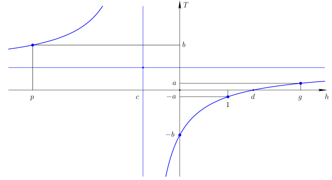
Figure 1. Homographic transformation for the computation of the integral $\,\int_{0}^{\,1}\!\!{{{\rm d}h}\over{\sqrt{\psi_{\lambda}(h)}}}$; case $\,p<0<1<g$.

If the sequence $\,\sigma_{0},\,\sigma_{1/2},\,\sigma_{1}\,$ is convex, id est if $\,\,\sigma_{1/2}-\sigma_{0}<\sigma_{1}-\sigma_{1/2}\,$, we have $\,\delta<0$, $\,a_{0}<0\,$ and the discriminant $\,\Delta\,$ introduced in (8) can be negative or positive. We begin by the case $\,\Delta<0\,$ and we have two conjugate roots for the polynomial $\,\psi_{\lambda}$. To fix the ideas, we set $\,p={1\over 2}\,(\sigma+i\,\sqrt{-\Delta})\,$ and $\,g={1\over 2}\,(\sigma-i\,\sqrt{-\Delta})\,$ with $\,\sigma\,$ introduced in Lemma 2.3.

Proposition 2.5.

With the notations recalled previously, in the case $\,\Delta<0\,$ with two conjugate roots, the computation of the integral $\,I\equiv\int_{0}^{\,1}\!\!{{{\rm d}h}\over{\sqrt{\psi_{\lambda}(h)}}}\,$ is splitted into three sub-cases:

(i) if $\,\sigma=1$, we have $\,I={{4}\over{\sqrt{|a_{0}|}\,\sqrt{-\Delta}}}\,K(m)\,$ with $\,m={{1}\over{\Delta}}<0$,

(ii) if $\,\sigma<1$, the integral $\,I\,$ can be computed with the following relations

$$\left\{\begin{array}[]{l}\widetilde{\Delta}={1\over 16}\,(\sigma^{2}-\Delta)\,\big{(}(\sigma-2)^{2}-\Delta\big{)}>0\,,\,\,c={{-1}\over{1-\sigma}}\,\big{(}\sqrt{\widetilde{\Delta}}+{1\over 4}\,(\sigma^{2}-\Delta)\big{)}<0\,,\\ a={{1}\over{1-2\,c}}\in(0,\,1)\,,\,\,b={{\sqrt{-\Delta}}\over{2\,c-\sigma}}\,,\,\,d=-a\,c>c\,,\,\,m=-{{a^{2}}\over{b^{2}}}<0\,,\\ I=2\,{{\sqrt{(1-a^{2})\,(b^{2}+1)}}\over{\sqrt{|a_{0}|}\,\,|b|\,\,(d-c)}}\,K(m)\,,\end{array}\right.$$

(iii) if $\,\sigma>1$, the integral $\,I\,$ is evaluated with the same relations that in the case (ii), except that we have now $\,c>0$, $\,a<0\,$ and $\,d<c$.

Proof.

First recall that

$\psi_{\lambda}(h)=|a_{0}|\,h\,(h-1)\,(h-p)\,(h-g)=(-a_{0})\,h\,(1-h)\,\big{(}(h-{{\sigma}\over{2}})^{2}-{{\Delta}\over{4}}\big{)}$.

(i) If $\,\sigma=1$, we make the change of variable: $\,v=h-{1\over 2}$. Then

$I={{1}\over{\sqrt{|a_{0}|}}}\,\int_{-1/2}^{1/2}{{{\rm d}v}\over{\sqrt{\big{(}{1\over 4}-v^{2}\big{)}\,\big{(}v^{2}-{{\Delta}\over{4}}\big{)}}}}$

and we can use the relation (7) with $\,a={1\over 2}\,$ and $\,b={{\sqrt{-\Delta}}\over{2}}$. Then

$I={{1}\over{\sqrt{|a_{0}|}}}\,{{4}\over{\sqrt{-\Delta}}}\,K(m)\,$ with $\,m=-{{1}\over{(-\Delta)}}={{1}\over{\Delta}}<0$.

(ii) If $\,\sigma<1$, we make an homographic change of variables $\,T(h)={{h-d}\over{h-c}}\,$ as in Proposition 2.4. We enforce now the conditions

$T(0)=-a$, $\,T(1)=a\,$ and $\,T\big{(}{{\sigma\pm i\,\sqrt{-\Delta}}\over{2}}\big{)}=\mp i\,b$

with real coefficients $\,a$, $\,b$, $\,c\,$ and $\,d$. If $\,\widetilde{h}\,$ is a root of $\,\psi_{\lambda}$, id est $\,\widetilde{h}\in\{0,\,1,\,p,\,g\}$, we have as previously $\,h-\widetilde{h}=(h-c)\,{{\widetilde{T}-T}\over{\widetilde{T}-1}}\,$ with $\,\widetilde{T}\in\{\pm a,\,i\,\pm b\}$. Thus $\,\psi_{\lambda}(h)=|a_{0}|\,(h-c)^{4}\,{{(a^{2}-T^{2})\,(T^{2}+b^{2})}\over{(1-a^{2})\,(1+b^{2})}}\,$ and we must enforce $\,a^{2}<1$. We have also $\,{\rm d}T={{d-c}\over{(h-c)^{2}}}\,{\rm d}h$. Then

$I={{1}\over{\sqrt{|a_{0}|}}}\,\int_{-a}^{\,a}\!{{(h-c)^{2}\,{\rm d}T}\over{d-c}}\,{{\sqrt{(1-a^{2})\,(1+b^{2})}}\over{(h-c)^{2}\,\sqrt{(a^{2}-T^{2})\,(T^{2}+b^{2})}}}$

$={{\sqrt{(1-a^{2})\,(1+b^{2})}}\over{\sqrt{|a_{0}|}\,(d-c)}}\,\int_{-a}^{\,a}\!{{{\rm d}T}\over{(a^{2}-T^{2})\,(T^{2}+b^{2})}}$ $=2\,{{\sqrt{(1-a^{2})\,(1+b^{2})}}\over{\sqrt{|a_{0}|}\,|b|\,(d-c)}}\,K(m)$

with $\,m=-{{a^{2}}\over{b^{2}}}\,$ due to the relation (7). The relation is established, but we have now to construct the homography $\,h\longmapsto T(h)$, taking into consideration the constraints $\,d>c\,$ and $\,a^{2}<1$. The constitutive relations $\,T(0)=-a$, $\,T(1)=a\,$ and $\,T\big{(}{{\sigma\pm i\,\sqrt{-\Delta}}\over{2}}\big{)}=\mp i\,b\,$ take the form

$\left\{\begin{array}[]{l}c-d=(-a-1)\,(0-c)=(a-1)\,(1-c)=\\ =(-i\,b-1)\,({{\sigma+i\,\sqrt{-\Delta}}\over{2}}-c)=(i\,b-1)\,({{\sigma-i\,\sqrt{-\Delta}}\over{2}}-c)\,.\end{array}\right.$

Then $\,{{i\,b+1}\over{i\,b-1}}={{i\,\sqrt{-\Delta}+(2\,c-\sigma)}\over{i\,\sqrt{-\Delta}-(2\,c-\sigma)}}$ and $\,b={{\sqrt{-\Delta}}\over{2\,c-\sigma}}$. We have also $\,{{a+1}\over{a-1}}={{1}\over{c}}-1\,$ then $\,a={{1}\over{1-2\,c}}$. We can write now the equation relative to the parameter $\,c$: $\,c\,(a+1)=(i\,b+1)\,(c-{{\sigma+i\,\sqrt{-\Delta}}\over{2}})$. But $\,(i\,b+1)\,(c-{{\sigma+i\,\sqrt{-\Delta}}\over{2}})={{(2\,c-\sigma)^{2}-\Delta}\over{2\,(2\,c-\sigma)}}\,$ and $\,a+1=2\,{{1-c}\over{1-2\,c}}$. An equation of degree 2 for the parameter $\,c\,$ is emerging:

$f(c)\equiv(1-\sigma)\,c+2\,{{\sigma^{2}-\Delta}\over{4}}\,c-{{\sigma^{2}-\Delta}\over{4}}=0\,.$

We remark that the constant term $\,{{\sigma^{2}-\Delta}\over{4}}\,$ is the square of the modulus of the two roots $\,p\,$ and $\,g$. So we have two roots $\,c_{-}\,$ and $\,c_{+}\,$ for the equation $\,f(c)=0$. We remark that $\,f({{\sigma}\over{2}})=-{1\over 4}\,\Delta\,(\sigma-1)<0\,$ in this case and $\,{{\sigma}\over{2}}\,$ is between the two roots. We have also $\,f({{1}\over{2}})={1\over 4}\,(1-\sigma)>0\,$ and $\,{1\over 2}\,$ is outside the two roots. We deduce the inequalities $\,c_{-}<0$, $\,c_{-}<{{\sigma}\over{2}}<c_{+}<{1\over 2}$, $\,c_{+}>0$. Before making a choice between the two numbers $\,c_{\pm}$, observe that we have $\,c-d=(a+1)\,c\,$ and $\,d=-a\,c$. Moreover $\,a={{1}\over{1-2\,c}}\,$ and the simplest choice is $\,a>0$. Then the condition $\,a^{2}<1\,$ take the form $\,a-1<0$, but $\,a-1={{2\,c}\over{1-2\,c}}$ and we must have $\,c<0$. Then $\,d>0\,$ and $\,c<0<d\,$; the condition $\,d-c>0\,$ is satisfied. The reduced discriminant $\,\widetilde{\Delta}\,$ is equal to $\,\big{(}{{\sigma^{2}-\Delta}\over{4}}\big{)}^{2}+(1-\sigma)\,\big{(}{{\sigma^{2}-\Delta}\over{4}}\big{)}={1\over 16}\,(\sigma^{2}-\Delta)\,\big{(}(\sigma-2)^{2}-\Delta\big{)}\,$ and is positive. Then $\,c=c_{-}={{-1}\over{1-\sigma}}\,\big{(}\sqrt{\widetilde{\Delta}}+{1\over 4}\,(\sigma^{2}-\Delta)\big{)}$.

(iii) If $\,\sigma>1$, the beginning of the previous proof is unchanged. But now the second order equation for the parameter $\,c\,$ takes the form

$\widetilde{f}(c)\equiv(\sigma-1)\,c-2\,{{\sigma^{2}-\Delta}\over{4}}\,c+{{\sigma^{2}-\Delta}\over{4}}=0\,.$

We still have $\,\widetilde{\Delta}={1\over 16}\,(\sigma^{2}-\Delta)\,\big{(}(\sigma-2)^{2}-\Delta\big{)}>0\,$ and the two roots $\,c_{\pm}\,$ have the same sign. We have now $\,\widetilde{f}({{\sigma}\over{2}})=-{1\over 4}\,\Delta\,(1-\sigma)<0\,$ and $\,{{\sigma}\over{2}}\,$ is still between the two roots. Moreover, $\,\widetilde{f}({{1}\over{2}})={1\over 4}\,(\sigma-1)>0\,$ and $\,{1\over 2}\,$ is outside the two roots. We deduce the inequalities $\,{1\over 2}<c_{-}<{{\sigma}\over{2}}<c_{+}$. Then whatever the choice between $\,c_{\pm}$, $\,2\,c-1>0\,$ and $\,a<0$. The condition $\,a^{2}<1\,$ imposes now $\,a+1>0\,$ and $\,a+1=2\,{{1-c}\over{1-2\,c}}\,$ is positive if and only of $\,1-c<0$. We observe also that $\,\widetilde{f}(1)=-\big{(}1-{{\sigma}\over{2}}\big{)}^{2}+{{\Delta}\over 4}<0$, then $\,c_{-}<1<c_{+}$. The choice $\,c_{+}\,$ is mandatory and we have $\,c=c_{+}={{1}\over{\sigma-1}}\,\big{(}\sqrt{\widetilde{\Delta}}+{1\over 4}\,(\sigma^{2}-\Delta)\big{)}$. ∎

Proposition 2.6.

With the notations recalled previously, in the case $\,\Delta>0\,$ with two real roots with the same sign, the computation of the integral $\,I\equiv\int_{0}^{\,1}\!\!{{{\rm d}h}\over{\sqrt{\psi_{\lambda}(h)}}}\,$ is splitted into two sub-cases:

(i) if $\,\sigma>2$, the integral $\,I\,$ can be evaluated according to

$\left\{\begin{array}[]{l}\Delta^{\prime}=4\,p\,g\,(p-1)\,(g-1)\,,\,\,b={{1}\over{(g-p)\,(g+p-1)}}\big{(}p\,(p-1)+g\,(g-1)+\sqrt{\Delta^{\prime}}\big{)}>1\,,\\ a=b\,(p-g)+p+g-1\,,\,\,c={{a+1}\over{2\,a}}\,,\,\,d=a\,c<c\,,\,\,m={{a^{2}}\over{b^{2}}}\,,\\ I=2\,{{\sqrt{(1-a^{2})\,(b^{2}-1)}}\over{\sqrt{|a_{0}|}\,\,b\,\,(c-d)}}\,K(m)\,,\end{array}\right.$

(ii) if $\,\sigma<0$, the integral $\,I\,$ is evaluated with the relations

$\left\{\begin{array}[]{l}\Delta^{\prime}=4\,p\,g\,(p-1)\,(g-1)\,,\,\,b={{1}\over{(g-p)\,(1-g-p)}}\big{(}p\,(p-1)+g\,(g-1)+\sqrt{\Delta^{\prime}}\big{)}>0\,,\\ a=b\,(p-g)+1-p-g\,,\,\,c=-{{1-a}\over{2\,a}}<0\,,\,\,d=-a\,c>0>c\,,\,\,m={{a^{2}}\over{b^{2}}}\,,\\ I=2\,{{\sqrt{(1-a^{2})\,(b^{2}-1)}}\over{\sqrt{|a_{0}|}\,\,|b|\,\,(d-c)}}\,K(m)\,,\end{array}\right.$

that are very similar to the first case. In both cases, we have $\,0<a<1<b$.

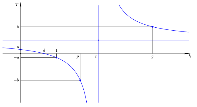
Figure 2. Homographic transformation for the computation of the integral $\,\int_{0}^{\,1}\!\!{{{\rm d}h}\over{\sqrt{\psi_{\lambda}(h)}}}$; case $\,0<1<p<g$.

Proof.

(i) In the case $\,\sigma>2$, we define an homographic function $\,T(h)={{h-d}\over{h-c}}\,$ represented in Figure 2 in order to enforce the inequalities $\,0<a<1<b\,$ and $\,0<d<1<p<c<g$. The constitutive relations beween the roots take now the form

$T(0)=a$, $\,T(1)=-a$, $\,T(p)=-b\,$ and $\,T(g)=b\,.$

We can write, with the same notations as previously, $\,h-\widetilde{h}=(h-c)\,{{\widetilde{T}-T}\over{\widetilde{T}-1}}\,$ and after mutiplying the four analogous factors, $\,\psi_{\lambda}(h)=|a_{0}|\,(u-c)^{4}\,{{(a^{2}-T^{2})\,(b^{2}-T^{2})}\over{(1-a^{2})\,(b^{2}-1)}}\,$ positive for $\,T^{2}<a^{2}<b^{2}$. Then

$I=\int_{a}^{\,-a}\!{{(h-c)^{2}}\over{\sqrt{|a_{0}|}\,(d-c)}}\,{{\sqrt{(1-a^{2})\,(b^{2}-1)}}\over{(h-c)^{2}\,\sqrt{(a^{2}-T^{2})\,(b^{2}-T^{2})}}}\,{\rm d}T$

$={{\sqrt{(1-a^{2})\,(b^{2}-1)}}\over{\sqrt{|a_{0}|}\,\,|b|\,\,(c-d)}}\,\int_{-a}^{\,a}{{{\rm d}T}\over{\sqrt{(a^{2}-T^{2})\,(b^{2}-T^{2})}}}$ $=2\,{{\sqrt{(1-a^{2})\,(b^{2}-1)}}\over{\sqrt{|a_{0}|}\,\,b\,\,(c-d)}}\,K(m)$

with $\,m={{a^{2}}\over{b^{2}}}\,$ due to the relation (5). The explicitaion of the coefficients $\,a\,$ to $\,d\,$ is conducted as previously: We first have

$0<c-d=(a-1)\,(0-c)=(-a-1)\,(1-c)=(-b-1)\,(p-c)\,(b-1)\,(g-c)$

and we get after some algebra conducted with the help of formal calculus, $\,d=a\,c$, $\,c={{a+1}\over{2\,a}}$, $\,a=b\,(p-g)+p+g-1\,$ and the parameter $\,b\,$ is a root of the second degree polynomial

${\check{f}}(b)\equiv(g-p)\,(g+p-1)\,b^{2}-2\,(p^{2}+g^{2}p-g)\,b+(g-p)\,(g+p-1)$

whose leading coefficient $\,(g-p)\,(g+p-1)\,$ is positive. The reduced associated discriminant

$\Delta^{\prime}=4\,p\,g\,(p-1)\,(g-1)$

is positive and we have just to compare the roots with the value $\,1\,$ because we want to enforce $\,b>1$. But $\,{\check{f}}(1)=4\,p\,(1-p)<0\,$ and $\ 1\,$ is between the two roots. So we have

$b={{1}\over{(g-p)\,(g+p-1)}}\big{(}p\,(p-1)+g\,(g-1)+\sqrt{\Delta^{\prime}}\big{)}>1$

and the first part of the proof is completed.

(ii) In the case $\,\sigma<0$, we follow the same method than previously. The homographic function $\,T(h)={{h-d}\over{h-c}}\,$ represented in Figure 3 and the parameters satisfy the conditions $\,0<a<1<b\,$ and $\,p<c<g<0<d<1$. We impose the following permutation between the roots:

$T(p)=b$, $\,T(g)=-b$, $\,T(0)=-a\,$ and $\,T(1)=a\,.$

Then we have as previously $\,\psi_{\lambda}(h)=|a_{0}|\,(u-c)^{4}\,{{(a^{2}-T^{2})\,(b^{2}-T^{2})}\over{(1-a^{2})\,(b^{2}-1)}}$, positive for $\,T^{2}<a^{2}<b^{2}$. Then we have

$I=\int_{-a}^{\,a}\!{{(h-c)^{2}}\over{\sqrt{|a_{0}|}\,(d-c)}}\,{{\sqrt{(1-a^{2})\,(b^{2}-1)}}\over{(h-c)^{2}\,\sqrt{(a^{2}-T^{2})\,(b^{2}-T^{2})}}}\,{\rm d}T=2\,{{\sqrt{(1-a^{2})\,(b^{2}-1)}}\over{\sqrt{|a_{0}|}\,\,|b|\,\,(d-c)}}\,K(m)\,$

with $\,m={{a^{2}}\over{b^{2}}}\,$ thanks to the relation (5). The explicitation of the coefficients $\,a$, $\,b$, $\,c\,$ and $\,d\,$ begin with the algebraic form

$0>c-d=(-a-1)\,(0-c)=(a-1)\,(1-c)=(b-1)\,(p-c)\,(-b-1)\,(g-c)$

of the conditions $\,T(p)=b$, $\,T(g)=-b$, $\,T(0)=-a\,$ and $\,T(1)=a$. We deduce that $\,d=-a\,c$, $\,c=-{{1-a}\over{2\,a}}$, $\,a=b\,(p-g)+1-p-g\,$ and the coefficient $\,b\,$ is solution of the equation of second degree

${\overline{f}}(b)\equiv(g-p)\,(1-g-p)\,b^{2}-2\,(p^{2}+g^{2}-p-g)\,b+(g-p)\,(1-g-p)\,.$

The reduced discriminant $\,\Delta^{\prime}\,$ is still given by the expression

$\Delta^{\prime}=4\,p\,g\,(p-1)\,(g-1)>0$.

The two roots are positive, we have $\,{\overline{f}}(1)=4\,g\,(1-g)>0\,$ and the only root greater that 1 is

$\,b={{1}\over{(g-p)\,(1-p-g)}}\big{(}p\,(p-1)+g\,(g-1)+\sqrt{\Delta^{\prime}}\big{)}\,.$

The proof of the proposition is completed. ∎

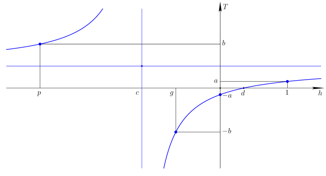
Figure 3. Homographic transformation for the computation of the integral $\,\int_{0}^{\,1}\!\!{{{\rm d}h}\over{\sqrt{\psi_{\lambda}(h)}}}$; case $\,p<g<0<1$.

$\bullet$ Third case: $\,\Sigma\,$ is a continuous positive fonction, affine in each interval $\,(0,\,{1\over 2})\,$ and $\,({1\over 2},\,1)$.

The function $\,\Sigma\,$ is defined by its values $\,\Sigma(0)=\sigma_{0}$, $\,\Sigma(\frac{1}{2})=\sigma_{1/2}\,$ and $\,\Sigma(1)=\sigma_{1}$. We introduce new parameters, still denoted by $\,\alpha\,$ and $\,\beta\,$ to represent the data:

$\sigma_{0}=\sigma_{1/2}\,(1-\alpha)\,$ and $\,\sigma_{1}=\sigma_{1/2}\,(1+\beta)\,.$

Then the inequalities $\,\alpha<1\,$ and $\,\beta>-1\,$ express the constraints $\,\sigma_{0}>0\,$ and $\,\sigma_{1}>0$. Moreover, $\,\sigma_{1/2}\,$ is positive.

Lemma 2.5.

If the continuous function $\,\Sigma\,$ defined on $\,(0,\,1)\,$ by its values

$\Sigma(0)=\sigma_{0}$, $\,\Sigma(\frac{1}{2})=\sigma_{1/2}$, $\,\Sigma(1)=\sigma_{1}$

is affine in each interval $\,(0,\,{1\over 2})\,$ and $\,({1\over 2},\,1)$, the function $\,\psi_{\lambda}\,$ defined by the conditions

${{{\rm d}^{2}\psi_{\lambda}}\over{{\rm d}h^{2}}}=1-2\,\lambda\,\Sigma\,\,$ and $\,\,\psi_{\lambda}(0)=\psi_{\lambda}(1)=0$

admits the following expression

$\psi_{\lambda}(h)=\left\{\begin{array}[]{l}\psi^{0}(h)\quad{\rm if}\,h\leq{1\over 2}\\ \psi^{1}(h)\qquad{\rm if}\,h\geq{1\over 2}\,,\end{array}\right.$

with

$\left\{\begin{array}[]{l}\psi^{0}(h)=-{2\over 3}\,\alpha\,\xi\,h^{3}+(\alpha\,\xi-\xi+1)\,h^{2}+\big{(}{{\beta-5\,\alpha}\over{12}}\,\xi+\xi-1\big{)}\,h\\ \psi^{1}(h)={2\over 3}\,\beta\,\xi\,(1-h)^{3}+(-\beta\,\xi-\xi+1)\,(1-h)^{2}+\big{(}{{5\,\beta-\alpha}\over{12}}\,\xi+\xi-1\big{)}\,(1-h)\,,\end{array}\right.$

with $\,\xi\equiv\lambda\,\sigma_{1/2}$. We have in particular $\,\psi_{\lambda}({1\over 2})={{\beta-\alpha}\over{24}}\,\xi+{1\over 4}\,(\xi-1)$. Moreover, if $\,\psi_{\lambda}\,$ is positive on the interval $\,(0,\,1)$,

${{{\rm d}\psi_{\lambda}}\over{{\rm d}h}}(0)={{\beta-5\,\alpha}\over{12}}\,\xi+\xi-1>0\,,\,\,{{{\rm d}\psi_{\lambda}}\over{{\rm d}h}}(1)=-\big{(}{{5\,\beta-\alpha}\over{12}}\,\xi+\xi-1\big{)}<0$.

Remark 1.

We observe that the expression of $\,\psi^{1}\,$ is obtained from the expression of $\,\psi^{0}\,$ by making the transformations $\,\alpha\longleftrightarrow(-\beta)\,$ and $\,h\longleftrightarrow(1-h)$.

Proof.

The function $\,\Sigma\,$ admits the algebraic expression:

$\Sigma(h)=\left\{\begin{array}[]{l}(2\,\alpha\,h-\alpha+1)\,\sigma_{1/2}\,\,\,\,{\rm if}\,h\leq{1\over 2}\\ (2\,\beta\,h-\beta+1)\,\sigma_{1/2}\,\,\,\,\,{\rm if}\,h\geq{1\over 2}\,.\end{array}\right.$

We integrate two times, enforce the conditions $\,\psi_{\lambda}(0)=\psi_{\lambda}(1)=0\,$ and impose the continuity of $\,\psi_{\lambda}\,$ and $\,{{{\rm d}\psi_{\lambda}}\over{{\rm d}h}}\,$ at the specific value $\,h={1\over 2}$. The result follows. ∎

We have to compute the integral $\,I\equiv\int_{0}^{\,1}\!\!{{{\rm d}h}\over{\sqrt{\psi_{\lambda}(h)}}}$. We have the following calculus:

$I=\int_{0}^{\,1/2}\!\!\!{{{\rm d}h}\over{\sqrt{\psi^{0}(h)}}}+\int_{1/2}^{\,1}\!{{{\rm d}h}\over{\sqrt{\psi^{1}(h)}}}=\int_{0}^{\,1/2}\!{{{\rm d}h}\over{\sqrt{\psi^{0}(h)}}}+\int_{0}^{\,1/2}\!{{{\rm d}h}\over{\sqrt{\psi^{1}(1-h)}}}$.

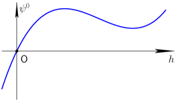
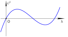
Figure 4. Contribution $\,\psi^{0}\,$ to the function $\,\psi_{\lambda}$. The case $\,\alpha>0\,$ is on the left and the case $\,\alpha<0\,$ is splitted into two figures: two complex roots in the middle and three real roots on the right.

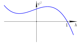
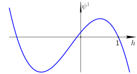
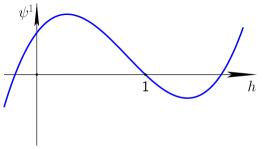
Figure 5. Contribution $\,\psi^{1}\,$ to the function $\,\psi_{\lambda}$. The case $\,\beta>0\,$ is splitted into two sub-cases: two complex roots on the left and three real roots in the middle; the case $\,\beta<0\,$ is presented on the right.

Due to the Remark 1, the determination of the second term relative to $\,\psi^{1}\,$ is very analogous to the term associated to $\,\psi^{0}$. In the following, we will concentrate essentially to the evaluation of the first integral $\,I_{0}\equiv\int_{0}^{\,1/2}\!\!\!{{{\rm d}h}\over{\sqrt{\psi^{0}(h)}}}$.

Proposition 2.7.

If $\,\alpha=0$, the integral $\,I_{0}\equiv\int_{0}^{\,1/2}\!\!{{{\rm d}h}\over{\sqrt{\psi^{0}(h)}}}\,$ admits several expressions parameterized by $\,\xi\equiv\lambda\,\sigma_{1/2}$:

(i) if $\,\xi=1$, then $\,\beta>0\,$ and $\,I_{0}=2\,\sqrt{{6}\over{\beta}}\,$,

(ii) if $\,\xi>1$, $\,I_{0}={{2}\over{\sqrt{\xi-1}}}\,\arctan\big{(}{{1}\over{\varphi_{0}}}\big{)}\,$ with $\,\varphi_{0}=\sqrt{1+{{\beta\,\xi}\over{6\,(\xi-1)}}}\,\,\,$ and

(iii) if $\,\xi<1$, $\,I_{0}={{1}\over{c\sqrt{b_{0}}}}\,\log{{\sqrt{c^{2}+2}+c}\over{\sqrt{c^{2}+2}-c}}\,$ with $\,b_{0}={{\beta}\over{12}}\,\xi+\xi-1>0\,$ and $\,c=\sqrt{{1-\xi}\over{b_{0}}}$.

Proof.

We have in this particular case $\,\psi^{0}(h)=-(\xi-1)\,h^{2}+\big{(}{{\beta}\over{12}}\,\xi+\xi-1\big{)}\,h$.

(i) If $\,\xi=1$, $\,\psi^{0}(h)={{\beta}\over{12}}\,h\,$ and $\,I_{0}=\sqrt{{12}\over{\beta}}\,\int_{0}^{\,1/2}\!{{{\rm d}h}\over{\sqrt{h}}}=\sqrt{{24}\over{\beta}}$.

(ii) If $\,\xi>1$, we write $\,\psi^{0}(h)=(\xi-1)\,h\,\Big{(}\big{(}1+{{\beta\,\xi}\over{12\,(\xi-1)}}\big{)}-h\Big{)}$. With $\,a\equiv 1+{{\beta\,\xi}\over{12\,(\xi-1)}}>0$, we make the classical change of variable $\,h\,(a-u)=\varphi^{2}\,h^{2}$. Then $\,\varphi^{2}={{a}\over{h}}-1\,$ and $\,2\,\varphi\,{\rm d}\varphi=-{{a}\over{h^{2}}}\,{\rm d}h$. If $\,h={1\over 2}$, then $\,\varphi=\varphi_{0}>0\,$ with $\,\varphi_{0}^{2}=2\,a-1=1+{{\beta\,\xi}\over{6\,(\xi-1)}}$. In consequence,

$I_{0}=\int_{+\infty}^{\varphi_{0}}\Big{(}{{-2\,h^{2}\,\varphi\,{\rm d}\varphi}\over{a\,\sqrt{\xi-1}}}\Big{)}\,{{1}\over{\varphi\,h}}$ $={{2}\over{\sqrt{\xi-1}}}\,\int_{\varphi_{0}}^{+\infty}\!{{{\rm d}\varphi}\over{1+\varphi^{2}}}$

$={{2}\over{\sqrt{\xi-1}}}\,\big{(}{{\pi}\over{2}}-\arctan(\varphi_{0})\big{)}$ $={{2}\over{\sqrt{\xi-1}}}\,\arctan\big{(}{{1}\over{\varphi_{0}}}\big{)}$

because $\,\varphi_{0}>0$.

(iii) If $\,\xi<1$, we can write $\,\psi^{0}(h)=b_{0}\,(h+c^{2}\,h^{2})\,$ with $\,b_{0}={{\beta}\over{12}}\,\xi+\xi-1>0\,$ and $\,c=\sqrt{{1-\xi}\over{b_{0}}}$. We make now the change of variable $\,h+c^{2}\,h^{2}=\theta^{2}\,h^{2}$. Then $\,\theta^{2}=c^{2}+{{1}\over{h}}>c^{2}\,$ and $\,2\,\theta\,{\rm d}\theta=-{{1}\over{h^{2}}}\,{\rm d}h$. Then

$I_{0}={{1}\over{\sqrt{b_{0}}}}\int_{+\infty}^{\sqrt{c^{2}+2}}(-2\,\theta\,h^{2}\,{\rm d}\theta)\,{{1}\over{\theta\,h}}$ $={{2}\over{\sqrt{b_{0}}}}\int_{\sqrt{c^{2}+2}}^{+\infty}\,h\,{\rm d}\theta={{2}\over{\sqrt{b_{0}}}}\int_{\sqrt{c^{2}+2}}^{+\infty}\,{{{\rm d}\theta}\over{\theta^{2}-c^{2}}}$

$={{1}\over{c\sqrt{b_{0}}}}\Big{[}\log{{\theta-c}\over{\theta+c}}\Big{]}_{\sqrt{c^{2}+2}}^{+\infty}$ $={{1}\over{c\sqrt{b_{0}}}}\,\log{{\sqrt{c^{2}+2}+c}\over{\sqrt{c^{2}+2}-c}}$.

The reader will observe that if $\,\xi\,$ tends to 1, each of the results proposed in (ii) and (iii) converge towards the expression proposed in (i). ∎

Proposition 2.8.

If $\,\alpha>0$, recall that $\,\psi^{0}(h)=-{2\over 3}\,\alpha\,\xi\,h^{3}+(\alpha\,\xi-\xi+1)\,h^{2}+\big{(}{{\beta-5\,\alpha}\over{12}}\,\xi+\xi-1\big{)}\,h$. It corresponds to the left part of Figure 4. The function $\,\psi^{0}\,$ admits three real roots and we set $\,\psi^{0}(h)\equiv a_{0}\,(h-r_{-})\,h\,(r_{+}-h)\,$ with $\,a_{0}={2\over 3}\,\alpha\,\xi>0\,$ and $\,r_{-}<0<r_{+}$. Then $\,I_{0}\equiv\int_{0}^{\,1/2}\!\!{{{\rm d}h}\over{\sqrt{\psi^{0}(h)}}}={{2}\over{\sqrt{a_{0}\,(-r_{-})}}}\,K(\varphi_{0},\,m)\,$ with $\,m={{r_{+}}\over{r_{-}}}<0\,$ and $\,\smash{\varphi_{0}=\arcsin\big{(}{{1}\over{\sqrt{2\,r_{+}}}}\big{)}}$.

Proof.

The explicitation of the algebraic expressions of $\,r_{-}\,$ and $\,r_{+}\,$ has no interest and is not detailed here. To compute $\,I_{0}$, we make the change of variables $\,h=r_{+}\,\sin^{2}\theta$. Then $\,{\rm d}h=2\,r_{+}\,\sin\theta\,\cos\theta$. Then

$\psi^{0}(h)\,=a_{0}\,(r_{+}\,\sin^{2}\theta-r_{-})\,r_{+}\,\sin^{2}\theta\,r_{+}\,\cos^{2}\theta$

$=a_{0}\,r_{+}^{2}\,\sin^{2}\theta\,\cos^{2}\theta\,(-r_{-})\,\big{(}1-{{r_{+}}\over{r_{-}}}\,\sin^{2}\theta\big{)}$

$=a_{0}\,(-r_{-})\,r_{+}^{2}\,\sin^{2}\theta\,\cos^{2}\theta\,(1-m\,\sin^{2}\theta)$

with $\,m={{r_{+}}\over{r_{-}}}<0$. Moreover, if $\,h={1\over 2}$, then $\,\theta=\varphi_{0}\,$ with $\,\sin^{2}\varphi_{0}={{1}\over{2\,r_{+}}}$. Then $\,I_{0}=\int_{0}^{\,\varphi_{0}}\!{{2\,{\rm d}\theta}\over{\sqrt{a_{0}\,(-r_{-})}}}\,{{1}\over{\sqrt{1-m\,\sin^{2}\theta}}}\,$ and the result is established. ∎

Proposition 2.9.

The case $\,\alpha<0$, corresponds to the middle and right pictures of Figure 4. Recall that $\,\psi^{0}(h)=-{2\over 3}\,\alpha\,\xi\,h^{3}+(\alpha\,\xi-\xi+1)\,h^{2}+\big{(}{{\beta-5\,\alpha}\over{12}}\,\xi+\xi-1\big{)}\,h$.

(i) If the polynomial $\,\psi^{0}(h)\,$ has two complex roots, we write it under the form $\,\psi^{0}(h)\equiv a_{0}\,h\,(h^{2}+\mu\,h+\zeta^{4})\,$ with $\,a_{0}={2\over 3}\,|\alpha|\,\xi>0\,$ and we have the inequality $\,\mu^{2}-4\,\zeta^{4}<0$; we introduce $\,m={1\over 2}-{{\mu}\over{4\,\zeta^{2}}}\,$ that satisfies $\,0<m<1\,$ and $\,\varphi_{0}=2\,\arctan\big{(}{{1}\over{\zeta\sqrt{2}}}\big{)}$. Then we have $\,I_{0}={{1}\over{\zeta\sqrt{a_{0}}}}\,K(\varphi_{0},\,m)$.

(ii) If the polynomial $\,\psi^{0}(h)\,$ has three real roots, we set $\,\psi^{0}(h)\equiv a_{0}\,h\,(r_{-}-h)\,(r_{+}-h)\,$ with $\,a_{0}={2\over 3}\,|\alpha|\,\xi>0\,$ and $\,0<r_{-}<r_{+}$; we consider $\,m={{r_{-}}\over{r_{+}}}\in(0,\,1)\,$ and $\,\varphi_{0}=\arcsin\big{(}{{1}\over{\sqrt{2\,r_{-}}}}\big{)}$. The integral $\,I_{0}\,$ is computed with the following expression: $\,I_{0}={{2}\over{\sqrt{a_{0}\,r_{+}}}}\,K(\varphi_{0},\,m)$.

Proof.

This proof is directly inspired by the book [1]. Nevertheless, we give the details herein for a complete explanation of the final relations.

(i) We operate the change of variable $\,h=\zeta^{2}\,t^{2}\,$ with $\,t=\tan{{\theta}\over{2}}$. Then

$\psi^{0}(h)\,=a_{0}\,\zeta^{2}\,t^{2}\,\big{(}\zeta^{4}\,(1+t^{4})+\mu\,\zeta^{2}\,t^{2}\big{)}$

$=a_{0}\,\zeta^{2}\,t^{2}\,\big{(}\zeta^{4}\,(1+t^{4})+\mu\,\zeta^{2}\,t^{2}\big{)}$

$=a_{0}\,\zeta^{6}\,t^{2}\,\big{(}(1+t^{2})^{2}-2\,t^{2}+{{\mu}\over{\zeta^{2}}}\,t^{2}\big{)}$

$=a_{0}\,\zeta^{6}\,t^{2}\,(1+t^{2})^{2}\,\big{[}1-\big{(}{1\over 2}-{{\mu}\over{4\,\zeta^{2}}}\big{)}\,{{4\,t^{2}}\over{(1+t^{2})^{2}}}\big{]}$.

Because the discriminant $\,\mu^{2}-4\,\zeta^{4}<0$ is negative, we have

${{|\mu|}\over{2\,\zeta^{2}}}<1\,$ and $\,-1<-{{\mu}\over{2\,\zeta^{2}}}<1$.

In other terms, $\,-{1\over 2}<-{{\mu}\over{4\,\zeta^{2}}}<{1\over 2}\,$ and $\,0<m\equiv{1\over 2}-{{\mu}\over{4\,\zeta^{2}}}<1$. We remark that $\,\sin\theta={{2\,t}\over{1+t^{2}}}\,$ and we get $\,\psi^{0}(h)=a_{0}\,\zeta^{6}\,t^{2}\,(1+t^{2})^{2}\,(1-m\,\sin^{2}\theta)$. We have also $\,{\rm d}h=2\,\zeta^{2}\,t\,(1+t^{2})\,{{{\rm d}\theta}\over{2}}\,$ and $\,{\rm d}h=\zeta^{2}\,t\,(1+t^{2})\,{\rm d}\theta$. With this change of variables, the upper bound is equal to $\,\varphi_{0}\,$ such that $\,\zeta^{2}\,\tan^{2}{{\varphi_{0}}\over{2}}={1\over 2}$, id est $\,\varphi_{0}=2\,\arctan\big{(}{{1}\over{\zeta\sqrt{2}}}\big{)}$. We can now achieve the calculus of the integral:

$I_{0}=\int_{0}^{\,1/2}\!\!{{{\rm d}h}\over{\sqrt{\psi^{0}(h)}}}$ $=\int_{0}^{\,\varphi_{0}}\!{{\zeta^{2}\,t\,(1+t^{2})\,{\rm d}\theta}\over{\sqrt{a_{0}}\,\zeta^{3}\,t\,(1+t^{2})\,\sqrt{1-m\,\sin^{2}\theta}}}$

$={{1}\over{\zeta\sqrt{a_{0}}}}\,\int_{0}^{\,\varphi_{0}}\!{{{\rm d}\theta}\over{\sqrt{1-m\,\sin^{2}\theta}}}={{1}\over{\zeta\sqrt{a_{0}}}}\,K(\varphi_{0},\,m)$.

(ii) If the polynomial $\,\psi^{0}(h)\equiv a_{0}\,h\,(r_{-}-h)\,(r_{+}-h)\,$ has three real roots, we set $\,h=r_{-}\,\sin^{2}\theta\,$ and

$\psi^{0}(h)=a_{0}\,\,r_{-}\,\sin^{2}\theta\,\,r_{-}\,\cos^{2}\theta\,(r_{+}-r_{-}\,\sin^{2}\theta)=a_{0}\,\,r_{-}^{2}\,\sin^{2}\theta\,\cos^{2}\theta\,\big{(}1-{{r_{-}}\over{t_{+}}}\,\sin^{2}\theta\big{)}$.

With $\,0<m\equiv{{r_{-}}\over{t_{+}}}<1$, we have $\,\psi^{0}(h)=a_{0}\,\,r_{-}^{2}\,\sin^{2}\theta\,\cos^{2}\theta\,(1-m\,\sin^{2}\theta)$. The upper bound $\,\varphi_{0}\,$ of the integral is associated to the relation $\,{1\over 2}=r_{-}\,\sin^{2}\varphi_{0}\,$ and $\,\varphi_{0}=\arcsin\big{(}{{1}\over{\sqrt{2\,r_{-}}}}\big{)}$. We have finally $\,,I_{0}=\int_{0}^{\,1/2}\!\!{{{\rm d}h}\over{\sqrt{\psi^{0}(h)}}}=\int_{0}^{\,\varphi_{0}}\!{{1}\over{\sqrt{a_{0}\,r_{+}}}}\,{{2\,{\rm d}\theta}\over{\sqrt{1-m\,\sin^{2}\theta}}}\,$ and the result is established. ∎

Remark 2.

As emphazized previously, the comutation of the second term

$I_{1}\equiv\int_{1/2}^{\,1}\!\!{{{\rm d}h}\over{\sqrt{\psi^{1}(h)}}}=\int_{0}^{\,1/2}\!\!{{{\rm d}h}\over{\sqrt{\psi^{1}(1-h)}}}$

of the global integral$\,I=I_{0}+I_{1}\,$ is obtained from the change of parameters $\,\alpha\longleftrightarrow(-\beta)\,$ in Propositions 2.7, 2.8 and 2.9. The different cases are illustrated on Figure 5.

3. Semi-analytical approximation

In this section, we revisit the results of Dellacherie et al. [4]. In this paper, they solved the equation $\,V^{\prime\prime}=\Sigma$, $\,V(0)=V(1)=0\,$ using a finite element approximation in the two-dimensional space $\,\{V_{a,b},\,V_{a,b}(h)=h(h-1)\,(a\,h+b)\}$, $\,\Sigma\,$ being the interpolation polynomial of degree 2 associated with $\,\sigma_{0}$, $\,\sigma_{1/2}\,$ and $\,\sigma_{1}$. We consider again this specific case to be able to compare with the results of section 2 and we add the case where $\,\Sigma\,$ is piecewise affine with the same approach.

$\bullet$ First semi-analytical case: $\,\Sigma\,$ is a P2 polynomial approximated by an affine function

More precisely, we consider the discrete vector space $\,W\,$ generated by the functions $\,h\longmapsto h\,(1-h)\,$ and $\,h\longmapsto h^{2}\,(1-h)$. Then we project the function $\,V(h)=\sigma_{0}\,(1-h)\,(1-2*h)+4\,\sigma_{1/2}\,h\,(1-h)+2\,\sigma_{1}\,h\,*(2*h-1)\,$ onto this space in the sense of least squares, as described in [6]. We obtain after the resolution of a $\,2\times 2\,$ linear system a new function $\,V\,$ of degree 3 that correcponds to an affine function. We obtain

$\widetilde{\Sigma}={1\over 5}\,\big{(}(3\,\sigma_{0}+4\,\sigma_{1/2}-2\,\sigma_{1})\,(1-h)+(-2\,\sigma_{0}+4\,\sigma_{1/2}+3\,\sigma_{1})\,h\big{)}$.

Then the process follows analogously to the first case with an affine function.

$\bullet$ First semi-analytical case: $\,\Sigma\,$ is a continuous positive fonction, affine in each interval $\,(0,\,{1\over 2})\,$ and $\,({1\over 2},\,1)$, approximated by an affine function

This case is analogous to the previous one, except that the initial function $\,\Sigma\,$ is piecewise affine:

$\Sigma(h)=\left\{\begin{array}[]{l}\sigma_{0}\,(1-2\,h)+2\,\sigma_{1/2}\,h\,\,\,\,\,\,\,\,\,\,\,\,{\rm if}\,h\leq{1\over 2}\\ 2\,\sigma_{1/2}\,(h-1)+\sigma_{1}\,(2\,h-1)\,\,\,\,\,\,\,{\rm if}\,h\geq{1\over 2}\,.\end{array}\right.$

We obtain after some elementary calculus

$\widetilde{\Sigma}={1\over 16}\,\big{(}(11\,\sigma_{0}+10\,\sigma_{1/2}-5\,\sigma_{1})\,(1-h)+(-5\,\sigma_{0}+10\,\sigma_{1/2}+11\,\sigma_{1})\,h\big{)}$.

And the end of the process is analogous to the previous case.

4. Numerical method

In this section, we describe a general numerical method (valid for any continuous funtion $\,\Sigma$) which solves directly the coupled problem (3) and finds an equation for computing $\,k_{eff}^{*}\,$ introduced in lemma 1.1. Note that this numerical method, unlike the one described in this Annex, does not use any coupling of codes. It needs only to sole one equation with one single real unknown.

Recall that problem (3) is

$$\left\{\begin{array}[]{l}-{{{\rm d}^{2}\varphi}\over{{\rm d}z^{2}}}+\varphi(z)=\lambda\,\Sigma\big{(}h(z)\big{)}\,\varphi(z),\,{{{\rm d}h}\over{{\rm d}z}}=\varphi(z)\,,\,0<z<1\,,\\ h(0)=0,\,h(1)=1,\,\varphi(0)=0,\,\varphi(1)=0,\,\lambda\geq 0,\,\varphi\geq 0.\end{array}\right.$$

We introduce a nonregular meshing $\,0=z_{0}<z_{1}<\,$… $<z_{N-1}<z_{N}=1\,$ of the interval $\,[0,\,1]\,$ and we set $\,\Delta z_{j+1/2}\equiv z_{j+1}-z_{j}\,$ for $\,j=1,\,$ … $\,,\,N$. We integrate the differential equation $\,{{{\rm d}h}\over{{\rm d}z}}=\varphi(z)\,$ with the Crank-Nicolson scheme:

$${{h_{j+1}-h_{j}}\over{\Delta z_{j+1/2}}}={1\over 2}\,\big{(}\varphi_{j}+\varphi_{j+1}\big{)}\,\,{\rm for}\,j=0,\,{\rm...}\,,\,N-1\,.$$

Then after two integrations, the first equation can be written as $\,\varphi_{j}=\sqrt{\psi_{\lambda}(h_{j})}\,$ and the Crank-Nicolson scheme takes the form

$${{h_{j+1}-h_{j}}\over{{1\over 2}\,\Big{(}\sqrt{\psi_{\lambda}(h_{j})}+\sqrt{\psi_{\lambda}(h_{j+1})}\,\Big{)}}}=\Delta z_{j+1/2}(\lambda)\,.$$

Note that the choice of the Crank-Nicolson algorithm allows to recover a discretization of each sub-problem (nemely the idealized neutronic one and the simplified thermo-hydraulic one). We impose the values $\,h_{j}\equiv\sin^{2}\big{(}{{\pi\,j}\over{2\,N}}\big{)}\,$ in order to take into account the singularities and two boundary conditions of the problem at $\,z=0\,$ and $\,z=1$. The notation $\,\Delta z_{j+1/2}(\lambda)\,$ in the right hand side of the previous relation is justified by the fact that if the numbers $\,h_{j}\,$ are given, the left hand side is a simple function of the scalar $\,\lambda$. The number $\,\lambda\,$ is a priori not known, but we have the natural relation $\,\sum_{j=0}^{N-1}\Delta z_{j+1/2}(\lambda)=1\,$ that takes the form

(9) $$\sum_{j=0}^{N-1}{{h_{j+1}-h_{j}}\over{{1\over 2}\Big{(}\sqrt{\psi_{\lambda}(h_{j})}+\sqrt{\psi_{\lambda}(h_{j+1})}\,\Big{)}}}=1\,.$$

Lemma 4.1.

Introduce $V$ the unique solution of $V^{\prime\prime}=\Sigma$, $V(0)=V(1)=0$. We have observed previously that $\,\psi_{\lambda}(h)=h\,(h-1)-2\,\lambda\,V(h)$. Define $\lambda_{*}=\mbox{max}_{[0,1]}\frac{h(h-1)}{V(h)}$.

(i) For $\lambda>\lambda_{*}$, $\psi_{\lambda}(h_{j})>0$

(ii) Equation (9) has a unique solution $\lambda\in(\lambda_{*},+\infty)$ when

$\sum_{j=0}^{N-1}{{h_{j+1}-h_{j}}\over{{1\over 2}\big{(}\sqrt{\psi_{\lambda_{*}}(h_{j})}+(\sqrt{\psi_{\lambda_{*}}(h_{j+1})}\,\big{)}}}\in{\mathbb{R}}_{+}>1$.

Proof.

(i) One notes that $V<0$ on $[0,1]$ thanks to $\Sigma\geq\Sigma_{*}$. Hence

$\psi_{\lambda}(h)=(-V(h))(\lambda-\frac{h(1-h)}{-V(h)})>0$ on $[0,1]$.

(ii) The limit of $\psi_{\lambda}(h_{i})$ is $+\infty$ for at least one value of $i$ when $\lambda\rightarrow+\infty$, the function $\psi_{\lambda}(h_{i})$ is increasing for any $i$, strictly increasing for $i\not=0,N$. The inequality $\,\sum_{j=0}^{N-1}{{h_{j+1}-h_{j}}\over{{1\over 2}\big{(}\sqrt{\psi_{\lambda_{*}}(h_{j})}+(\sqrt{\psi_{\lambda_{*}}(h_{j+1})}\,\big{)}}}>1\,$ (where $h_{j}$ or $h_{j+1}$ can be a point of maximum of $\frac{h(h-1)}{V(h)}$ in which case the sum is $+\infty$) and $\lambda\longmapsto\sum_{j=0}^{N-1}{{h_{j+1}-h_{j}}\over{{1\over 2}\big{(}\sqrt{\psi_{\lambda_{*}}(h_{j})}+\sqrt{\psi_{\lambda_{*}}(h_{j+1})}\,\big{)}}}$ strictly decreasing yields the result. ∎

For a fixed discretization with $\,N\,$ meshes, a Newton algorithm can be implemented without difficulty. With this procedure, we recover on one hand an approximated value $\,\lambda_{N}\,$ of the unknown $\,\lambda\,$ and on the other hand the entire approximate solution of the problem $\,h_{j}\approx h(x_{j})\,$ and $\,\varphi_{j}\approx\sqrt{\psi_{\lambda}(h_{j})}$. Observe that at convergence of the Newton algorithm, the abscissas $\,x_{j}\,$ are a function of the solution $\,\lambda_{N}\,$ and the converged space mesh is a result of the problem. This coupled problem can be reduced to a single equation with only one real variable even after discretization!

5. Numerical results

They are presented in Figures 6 and 7. They correspond to the decreasing data $\,\sigma_{0}=8$, $\,\sigma_{1/2}=6\,$ and $\,\sigma_{1}=3$. We obtain the following exact values for the scalar parameter: $\,\lambda=1.89036\,$ in the decoupled case (case 0), $\,\lambda=1.99533\,$ in the affine case (case 1), $\,\lambda=1.86593\,$ in the parabolic case (case 2), $\,\lambda=1.89454\,$ in the piecewise affine case (case 3) and $\,\lambda=1.85769\,$ in the parabolic case approached by an affine functions (semi-analytical case 1) $\,\lambda=1.88614\,$ in the piecewise affine case projected on affine functions (semi-analytical case 2). For each of these six cases, our numerical approach gives converging results at second order accuracy for the parameter $\,\lambda$.

If one wants to relate these calculations with the usual problemes solved in the neutronics world, by homogeneity, it is enough to consider the values $\,\sigma_{0}=14.92744$, $\,\sigma_{1/2}=11.19558\,$ and $\,\sigma_{1}=5.59779$. For this case, the following exact values for $\,k_{eff}^{*}\,$ are $\,0.98708\,$ in the decoupled case (case 0), $\,0.93515\,$ in the affine case (case 1), $\,1.00000\,$ in the parabolic case (case 2), $\,0.98490\,$ in the piecewise affine case (case 3), $\,1.00444\,$ in the parabolic case approached by an affine functions (semi-analytical case 1) and $\,0.98928\,$ in the piecewise affine case projected on affine functions (semi-analytical case 2). This investigation shows that some times, the exigence of accuracy of the operational calculations [11] could be lightened.

  

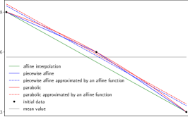
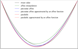
Figure 6. function $\,\Sigma\,$ on the left, $\,V\,$ on the right.

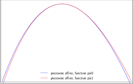
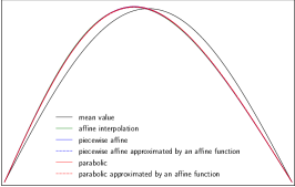
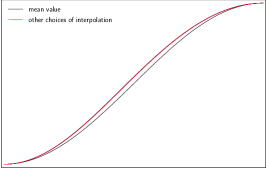
Figure 7. functions $\,h\longmapsto\psi^{0}(h)\,$ and $\,h\longmapsto\psi^{1}(h)\,$ on the left, $\,z\longmapsto\varphi(z)\,$ in the middle and $\,z\longmapsto h(z)\,$ on the right.

6. Conclusion

We considered in this paper a simplified idealized one-dimensional coupled model for neutronics and thermo-hydraulics. A numerical method allowing to find the unique solution of this coupled model (uniqueness of the multiplication factor $\,k_{eff}\,$ and of the neutron flux profile) is based on the Crank-Nicolson scheme. Simultaneously, special function (incomplete elliptic integrals) are used for finding analytic solutions for five different methods of representation of the fission cross section known at three points. Both methods match perfectly. We observe important differences in the multiplication factor, even if the neutron flux is really similar.
Future work concerns, for example, increasing the number of discretization points of cross sections.

Annex: Coupling algorithm

We derived in this paper an approach based on the use of an equation which takes into account the multiphysics of the problem, indeed constructing our method for solving numerically the problem using a totally coupled equation.

However, the method traditionally used for solving such a problem is based on the coupling of existing codes solving each equation.

The aim of this Annex is to describe the best result that can be obtained so far for such a coupling algorithm, and to give a sufficient condition for the convergence of this coupling algorithm. It is a follow-up of a first version (unpublished, on hal, see [5]) of this numerical coupling problem. Observe that the numerical method described in Section 4 converges with very weak hypotheses on $\Sigma$, while the coupling algorithm uses a very sharp condition on the coefficients and on the initial point chosen (see Lemma 6.3)

The equation coming from the thermohydraulics model is here $h^{\prime}(z)=(h_{s}-h_{e})\phi(z)$, where $\int_{0}^{1}\phi(z)dz=1$ (in the reduced model described in the paper $h_{s}-h_{e}=1$ and one chooses to use this value from now on).

This traditional numerical procedure, which couples codes rather than models reads as follows:

1. $\Sigma=\Sigma(0)\Rightarrow\lambda_{0},\phi_{0},$ with $\int_{0}^{1}\phi_{0}(z)dz=1$

2. for $n\geq 1$, $h_{n}$ solves $h^{\prime}_{n}(z)=\phi_{n-1}(z)$,

3. for $n\geq 1$, $\lambda_{n}$ is the smallest generalized eigenvalue of the problem $(-\frac{d^{2}}{dz^{2}}+1)\phi_{n}=\lambda_{n}\Sigma(h_{n})\phi_{n}$ and $\phi_{n}$ is the unique associated solution satisfying $\int_{0}^{1}\phi_{n}(z)dz=1$.

Denote by $R(h)=(\Sigma(h))^{-\frac{1}{2}}$.

Observe that the unique solution $(h_{*},\phi_{*},\lambda_{*})$ obtained in Lemma 1.2 for the system (3) satisfies that

• the real $\lambda_{*}$ is the smallest eigenvalue of $R(h_{*})(-\frac{d^{2}}{dz^{2}}+1)R(h_{*})$

• An associated eigenvector $\psi_{*}$ is $\psi_{*}=\sqrt{\Sigma(h_{*})}\phi_{*}$, with $\int_{0}^{1}\phi_{*}(z)dz=1$

• one has $h_{*}(z)=\int_{0}^{z}\phi_{*}(z^{\prime})dz^{\prime}$.

When treating only the differential equation of the system (3), one has, for the equation for $\phi,\lambda$, assuming that $\Sigma(h)$ is a $C^{1}$ function bounded below by $\Sigma_{0}>0$

Lemma 6.1.

1. The set of values of $\lambda$ such that $(-\frac{d^{2}}{dz^{2}}+1)\phi=\lambda\Sigma(h)\phi$ has a non trivial $H^{1}_{0}$ solution $\phi$ is the set of values of $\lambda$ such that $\lambda$ is in the spectrum of $R(h)(-\frac{d^{2}}{dz^{2}}+1)R(h)$ or $\frac{1}{\lambda}$ is in the spectrum of

   $$\mathcal{L}_{h}=R(h)^{-1}(-\frac{d^{2}}{dz^{2}}+1)^{-1}R(h)^{-1}$$

2. For $h\in C^{0}$, the operator $\mathcal{L}_{h}$ is self-adjoint compact on $L^{2}([0,1])$, hence its spectrum is a countable sequence of eigenvalues $\mu_{j}(h)$, decreasing to 0 when $j\rightarrow+\infty$.

One denotes by $\mu(h)$ the largest eigenvalue of $\mathcal{L}_{h}$. One denotes $\psi_{h}$ its associated unique eigenvector such that $\int_{0}^{1}\sqrt{\Sigma(h(z))}\psi_{h}(z)dz=1$.

We shall use the following regularity result, for $(h,{\tilde{h}})$ two $C^{1}$ functions satisfying the end conditions $h(0)={\tilde{h}}(0)=0,h(1)={\tilde{h}}(1)=1$.
Assume $M_{0}>0$ be given and denote by $B\subset C^{0}([0,1])$ such that $|h|_{C^{0}}\leq M_{0}$ for all $h\in B$. Denote by $C_{0}$ such that, for all $h,{\tilde{h}}$ in $B$, $|\sqrt{\Sigma(h)}-\sqrt{\Sigma({\tilde{h}})}|\leq C_{0}|h-{\tilde{h}}|_{C^{0}}$. Denote by $N$ the norm of $||P_{0}^{-1}||_{\mathcal{L}(L^{2}([0,1]),L^{2}([0,1]))}$, $P_{0}^{-1}$ being the inverse of $-\frac{d^{2}}{dz^{2}}+1$ from $L^{2}([0,1])$ to $H^{1}_{0}([0,1])\subset L^{2}([0,1])$.

Proposition 6.1.

There exists $\epsilon_{0}>0$ such that for all $h,{\tilde{h}}$ in $B$ such that $|h-{\tilde{h}}|_{C^{0}}\leq\epsilon_{0}$:

• Control of the approximation of the difference of the largest eigenvalue for $h$ and for ${\tilde{h}}$ $\mu(h)-\mu({\tilde{h}})$ at order 2:

  $$|(\mu(h)-\mu({\tilde{h}}))-2||\Sigma||_{\infty}^{\frac{1}{2}}NC_{0}|h-{\tilde{h}}|_{C^{0}}|\leq\frac{8||\Sigma||_{\infty}(NC_{0})^{2}|h-{\tilde{h}}|_{C^{0}}^{2}}{\mu_{2}(h)-\mu(h)},$$

• control of the difference of the normalized eigenvectors

  $$|\psi_{h}-\psi_{{\tilde{h}}}|\leq\frac{4||\Sigma||_{\infty}^{\frac{1}{2}}NC_{0}}{\mu_{2}(h)-\mu(h)}|h-{\tilde{h}}|_{C^{0}}^{2}|\psi_{h}|_{L^{2}}.$$

Let $K$ be the constant

$$K=2M\Sigma_{\infty}^{\frac{1}{2}}+\frac{C_{0}}{\Sigma_{0}^{\frac{1}{2}}}.$$

Lemma 6.2.

The sequence $h_{n},\lambda_{n}$ described in the numerical procedure satisfies, for $|h_{n}-h_{n-1}|_{C^{0}}$ small enough such that $|h_{n+1}-h_{n}|_{C^{0}}\leq\frac{\mu_{2}(h_{n})-\mu(h_{n})}{8NC_{0}}$

$$|h_{n+1}-h_{n}|_{C^{0}}\leq K||\psi_{n}||_{L^{2}}|h_{n}-h_{n-1}|_{C^{0}}$$

$$|\mu_{n+1}-\mu_{n}|\leq 4\Sigma_{\infty}NC_{0}|h_{n+1}-h_{n}|_{C^{0}}.$$

We deduce immediately

Lemma 6.3.

This algorithm converges under the sufficient condition

$$K||\psi_{n}||_{L^{2}}\leq\epsilon_{*}<1$$

for all $n\geq n_{0}$.

It is, evidently, a very strong condition, which is fulfilled when $C_{0}$ is small and when $||\psi_{n}||_{L^{2}}$ is bounded uniformly in $n$ for $n$ large enough (meaning also that one is in a neighborhood of the solution).

Proof of Proposition 6.1.

Consider the operator $\mathcal{L}_{h}$. The operator $S(h)$: $\psi\rightarrow\sqrt{\Sigma(h(x))}\psi$ is bounded from $L^{2}([0,1])$ to $L^{2}([0,1])$, the operator $P_{0}^{-1}$ is continuous from $L^{2}([0,1])$ to $H^{1}_{0}([0,1])$, hence is compact from $L^{2}([0,1])$ to $L^{2}([0,1])$, hence the composition by $S$ of $P_{0}^{-1}S$ is compact on $L^{2}([0,1])$. It has thus a discrete spectrum.

We write $L^{2}([0,1])=\mathbb{R}\psi_{h}\oplus{\tilde{H}}$ and we consider the decomposition of $S({\tilde{h}})P_{0}^{-1}S({\tilde{h}})$ on this decomposition of spaces. It writes, for any ${\tilde{h}}\in C^{0}([0,1])$

$$\left(\begin{array}[]{cc}A_{11}({\tilde{h}})&A_{12}({\tilde{h}})\\ A_{21}({\tilde{h}})&A_{22}({\tilde{h}})\end{array}\right).$$

Observe that $A_{12}(h)=0$, $A_{21}(h)=0$.

One has
$\mathcal{L}_{\tilde{h}}-\mathcal{L}_{h}=S({\tilde{h}})P_{0}^{-1}S({\tilde{h}})-S(h)P_{0}^{-1}S(h)$

$=S({\tilde{h}})P_{0}^{-1}(S({\tilde{h}})-S(h))+(S({\tilde{h}})-S(h))P_{0}^{-1}S(h),$ which implies

$$||\mathcal{L}_{\tilde{h}}-\mathcal{L}_{h}||_{\mathcal{L}(L^{2},L^{2})}\leq 2\Sigma_{\infty}^{\frac{1}{2}}C_{0}N|h-{\tilde{h}}|_{C^{0}}\,.$$

For $h-{\tilde{h}}$ small enough in $C^{0}$, the smallest eigenvalue of $S({\tilde{h}})P_{0}^{-1}({\tilde{h}})$, that is $\mu({\tilde{h}})$, satisfies the identity

(10) $$A_{11}({\tilde{h}})-\mu({\tilde{h}})-A_{12}({\tilde{h}})(A_{22}({\tilde{h}})-\mu({\tilde{h}})I)^{-1}A_{21}({\tilde{h}})=0.$$

Recall that, thanks to the inequality on $\mathcal{L}_{\tilde{h}}-\mathcal{L}_{h}$, one has

$$|A_{11}({\tilde{h}})-A_{11}(h)|\leq 2\Sigma_{\infty}^{\frac{1}{2}}C_{0}N|h-{\tilde{h}}|_{C^{0}},$$

$$||A_{12}({\tilde{h}})||_{\mathcal{L}(L^{2},L^{2})}\leq 2\Sigma_{\infty}^{\frac{1}{2}}C_{0}N|h-{\tilde{h}}|_{C^{0}},||A_{21}({\tilde{h}})||_{\mathcal{L}(L^{2},L^{2})}\leq 2\Sigma_{\infty}^{\frac{1}{2}}C_{0}N|h-{\tilde{h}}|_{C^{0}},$$

and that the smallest eigenvalue of $A_{22}({\tilde{h}})$ is $\mu_{2}({\tilde{h}})$, hence $A_{22}({\tilde{h}})-\mu I\geq({\tilde{\mu}}_{2}(h)-\mu I)$ (on $L^{2}([0,1])$). Hence, from (10)

$|A_{11}({\tilde{h}})-\mu({\tilde{h}})|\leq(2\Sigma_{\infty}^{\frac{1}{2}}C_{0}N|h-{\tilde{h}}|_{C^{0}})^{2}||(A_{22}({\tilde{h}})-\mu({\tilde{h}})I)^{-1}||_{\mathcal{L}(L^{2},L^{2})}$

$\leq\frac{4\Sigma_{\infty}(C_{0}N)^{2}}{\mu_{2}({\tilde{h}})-\mu({\tilde{h}})}|h-{\tilde{h}}|_{C^{0}}^{2}.$
There exists $\epsilon_{0}>0$ such that for $|h-{\tilde{h}}|_{C^{0}}\leq\epsilon_{0}$, $\mu_{2}({\tilde{h}})-\mu({\tilde{h}})\geq\frac{\mu_{2}(h)-\mu(h)}{2}$, hence the required estimate for $A_{11}({\tilde{h}})-\mu({\tilde{h}})$, which implies the estimate for

$$\mu({\tilde{h}})-\mu(h)=\mu({\tilde{h}})-A_{11}({\tilde{h}})+A_{11}({\tilde{h}})-A_{11}(h).$$

An eigenvector associated to $\mu({\tilde{h}})$ writes $\psi_{h}+r$, where

$$\left(\begin{array}[]{cc}A_{11}({\tilde{h}})-\mu({\tilde{h}})&A_{12}({\tilde{h}})\\ A_{21}({\tilde{h}})&A_{22}({\tilde{h}})-\mu({\tilde{h}})I\end{array}\right)\left(\begin{array}[]{l}\psi_{h}\\ r\end{array}\right)=0,$$

hence one gets

$$r=-(A_{22}({\tilde{h}})-\mu({\tilde{h}})I)^{-1}A_{21}({\tilde{h}})\psi_{h}.$$

One has thus $\psi_{{\tilde{h}}}=k(\psi_{h}+r)$, where $k^{-1}=\int_{0}^{1}\sqrt{\Sigma({\tilde{h}})}(\psi_{h}(z)+r(z))dz$. One has $\psi_{{\tilde{h}}}-\psi_{h}=(k-1)\psi_{h}+kr$, and $k-1=k(1-\frac{1}{k})=k(\int_{0}^{1}\sqrt{\Sigma(h)}\psi_{h}(z)dz-\int_{0}^{1}\sqrt{\Sigma({\tilde{h}})}(\psi_{h}(z)+r(z))dz)$.
Let $M=\frac{C_{0}}{\Sigma_{0}^{\frac{1}{2}}}+\frac{8\Sigma_{\infty}^{\frac{1}{2}}C_{0}N}{\mu_{2}(h)-\mu(h)}$. Note that

$$\frac{k-1}{k}=\int_{0}^{1}\frac{\sqrt{\Sigma(h)}-\sqrt{\Sigma({\tilde{h}})}}{\sqrt{\Sigma(h)}}\sqrt{\Sigma(h)}\psi_{h}(z)dz+\int_{0}^{1}\sqrt{\Sigma({\tilde{h}})}r(z)dz,$$

$$|\frac{\sqrt{\Sigma(h)}-\sqrt{\Sigma({\tilde{h}})}}{\sqrt{\Sigma(h)}}|\leq\frac{C_{0}}{\Sigma_{0}^{\frac{1}{2}}}|h-{\tilde{h}}|_{C^{0}},$$

$$||r||_{L^{2}}\leq\frac{4\Sigma_{\infty}^{\frac{1}{2}}C_{0}N|h-{\tilde{h}}|_{C^{0}}}{\mu_{2}(h)-\mu(h)}||\psi_{h}||_{L^{2}}.$$

For $\big{(}\frac{C_{0}}{\Sigma_{0}^{\frac{1}{2}}}+\frac{4\Sigma_{\infty}^{\frac{1}{2}}C_{0}N}{\mu_{2}(h)-\mu(h)}\big{)}||\psi_{h}||_{L^{2}}|h-{\tilde{h}}|_{C^{0}}\leq\frac{1}{2}$, one has the inequalities $k\leq 2$ and

$$k-1\leq 2(\frac{C_{0}}{\Sigma_{0}^{\frac{1}{2}}}+\frac{4\Sigma_{\infty}^{\frac{1}{2}}C_{0}N}{\mu_{2}(h)-\mu(h)})||\psi_{h}||_{L^{2}}|h-{\tilde{h}}|_{C^{0}}.$$

The inequality

(11) $$||\psi_{{\tilde{h}}}-\psi_{h}||_{L^{2}}\leq 2M|h-{\tilde{h}}|_{C^{0}}||\psi_{h}||_{L^{2}}$$

follows. The proposition is proven. $\square$ Note that $1\leq\sqrt{\int_{0}^{1}\Sigma(h(z))dz}||\psi_{h}||_{L^{2}}\leq\Sigma_{\infty}^{\frac{1}{2}}||\psi_{h}||_{L^{2}}$, which gives only a lower bound for $||\psi_{h}||_{L^{2}}$.
Proof of Lemma 6.2
One has, of course, $\frac{1}{\lambda_{n}}=\mu(h_{n})$, and $\phi_{n}=\sqrt{\Sigma(h_{n})}\psi_{n}$, and $h_{n+1}(z)=\int_{0}^{z}\phi_{n}(s)ds$. One has $h_{n+1}(z)-h_{*}(z)=\int_{0}^{z}(\phi_{n}(s)-\phi_{*}(s))ds$, hence $h_{n+1}-h_{*}$ is continuous, and
$|h_{n+1}-h_{*}|_{C^{0}}\leq|\int_{0}^{z}\Big{[}\sqrt{\Sigma(h_{*}(s))}(\psi_{n}(s)-\psi_{*}(s))+\sqrt{\Sigma(h_{n}(s))}[\sqrt{\frac{\Sigma(h_{n})}{\Sigma(h_{*})}}-1]\psi_{*}(s)\Big{]}ds|$

$\leq(2M\Sigma_{\infty}^{\frac{1}{2}}+\frac{C_{0}}{\Sigma_{0}^{\frac{1}{2}}})|h_{n}-h_{*}|_{C^{0}}||\psi_{n}||_{L^{2}}.$

In a similar way, $(h_{n+1}-h_{n})(z)=\int_{0}^{z}(\phi_{n}(s)-\phi_{n-1}(s))ds$, which yields the estimate $|h_{n+1}-h_{n}|_{C^{0}}\leq(2M\Sigma_{\infty}^{\frac{1}{2}}+\frac{C_{0}}{\Sigma_{0}^{\frac{1}{2}}})|h_{n}-h_{n-1}|_{C^{0}}||\psi_{n-1}||_{L^{2}}$, and

$$|\frac{1}{\lambda_{n+1}}-\frac{1}{\lambda_{n}}|\leq 2\Sigma_{\infty}^{\frac{1}{2}}NC_{0}|h_{n+1}-h_{n}|_{C^{0}}+\frac{8\Sigma_{\infty}(NC_{0})^{2}|h_{n+1}-h_{n}|_{C^{0}}^{2}}{\mu_{2}(h_{n})-\mu(h_{n})}.$$

Under the hypothesis of Lemma 6.2 on $h_{n+1}-h_{n}$, we deduce the estimate on $|\frac{1}{\lambda_{n+1}}-\frac{1}{\lambda_{n}}|$. $\square$

References

- [1] M. Abramowitz and I. A. Stegun – Handbook of Mathematical Functions with Formulas, Graphs, and Mathematical Tables, National Bureau of Standards, Applied Mathematics Series - 55, June 1964.
- [2] E.A. Coddington and N. Levinson – Theory of ordinary differential equations – Chapter 8, International series in pure and applied mathematics, McGraw-Hill, 1955.
- [3] S. Dellacherie – “On a low Mach nuclear core model” – ESAIM:PROCs, 35, pp. 79-106, 2012.
- [4] S. Dellacherie, E. Jamelot, O. Lafitte, M. Riyaz – “Numerical results for the coupling of a simple neutronics diffusion model and a simple hydrodynamics low mach number model without coupling codes, 18th International Symposium on Symbolic and Numeric Algorithms for Scientific Computing (SYNASC 2016), pages 119-124, DOI: 10.1109/SYNASC40771.2016.
- [5] S. Dellacherie and O. Lafitte – “Une solution explicite monodimensionnelle d’un modèle simplifié de couplage stationnaire thermohydraulique-neutronique”, https://hal.archives-ouvertes.fr/hal-01263642v1, 2012.
- [6] S. Dellacherie and O. Lafitte – “Une solution explicite monodimensionnelle d’un modèle simplifié de couplage stationnaire thermohydraulique-neutronique”, Annales mathématiques du Québec, volume 41, pages 221–264, 2017.
- [7] S. Dellacherie, E. Jamelot and O. Lafitte – “A simple monodimensional model coupling an enthalpy transport equation and a neutron diffusion equation”, Mathematics Letters, (62) 2016, pp. 35-41.
- [8] F. Dubois and O. Lafitte – “An analytic and symbolic analysis of a coupled thermo-neutronic problem”, 23rd International Symposium on Symbolic and Numeric Algorithms for Scientific Computing (SYNASC), pp. 61-65, 2021, IEEE:doi 10.1109/SYNASC54541.2021.00022.
- [9] J.J. Duderstadt and L.J. Hamilton – Nuclear Reactor Analysis – Wiley & Sons, New York, 1976.
- [10] W. Stein and D. Joyner – “SAGE: System for Algebra and Geometry Experimentation”, ACM SIGSAM Bulletin, volume 39, number 2, pages 61-64, 2005. Sagemath, with more than 600 contributors around the world, is a free open-source mathematics software system licensed under the GPL, www.sagemath.org.
- [11] M. Tiberga, R. Gonzalez Gonzaga de Oliveira, E. Cervi, J.A. Blanco, S. Lorenzi, M. Aufiero, D. Lathouwers, P. Rubiolo – “Results from a multi-physics numerical benchmark for codes dedicated to molten salt fast reactors”, Annals of Nuclear Energy (142) 2020, pp. 107428.