Low-order moments of the velocity gradient in homogeneous compressible turbulence

Abstract

We derive from first principles analytic relations for the second and third order moments of the velocity gradient $m_{ij}=\frac{\partial u_{i}}{\partial x_{j}}$ in compressible turbulence, which generalize known relations in incompressible flows. These relations, although derived for homogeneous flows, hold approximately for a mixing layer. We also discuss how to apply these relations to determine all the second and third moments of the velocity gradient experimentally.

1 Introduction

In high Reynolds number flows, the velocity field, $\mathbf{u}$, develops very sharp gradients (Frisch, 1995; Sreenivasan & Antonia, 1997), resulting in extremely large fluctuations of the velocity gradient $\mathbf{m}$, or $m_{ij}=\frac{\partial u_{i}}{\partial x_{j}}$. For this reason, an accurate description of the velocity gradient is essential to understand the small-scale properties of turbulence (Meneveau, 2011). In the case of incompressible turbulence, much emphasis has been put on enstrophy, defined as $\frac{1}{2}\omega_{i}\omega_{i}$, where ${\bm{\omega}}=\nabla\times\mathbf{u}$. Its amplification rate, known as vortex stretching, $\omega_{i}s_{ij}\omega_{j}$, where $\mathbf{s}$ is the symmetric part of $\mathbf{m}$, or the rate of strain tensor, have been thoroughly studied to investigate the production of small scales in the flow (Tsinober, 2009; Buaria et al., 2020). It should be kept in mind that a thorough description of small scales involves the full tensor $\mathbf{m}$, and not just vorticity (Meneveau, 2011).

Two remarkable constraints on the second and third moments of $\mathbf{m}$ have been established by Betchov (1956) for homogeneous and incompressible flows:

$$\langle\mathrm{tr}(\mathbf{m}^{2})\rangle=0\quad{\rm and}\quad\langle\mathrm{tr}(\mathbf{m}^{3})\rangle=0,$$ (1)

where $\langle\,\rangle$ denotes ensemble average. In addition, when the flow is isotropic, the identities (1) lead to remarkable simplifications, allowing the second and third order moments of the velocity gradient tensors $\mathbf{A}^{(2)}=\langle\mathbf{m}^{2}\rangle$ and $\mathbf{A}^{(3)}=\langle\mathbf{m}^{3}\rangle$ to be expressed in terms of only one scalar quantity (Pope, 2000). This implies that in an isotropic flow, $\mathbf{A}^{(2)}$ and $\mathbf{A}^{(3)}$ can be completely determined from the measurement of only one component of the velocity gradient tensor, e.g., using hot-wire probes. Although strictly zero in homogeneous incompressible flows, the values of $\langle\mathrm{tr}(\mathbf{m}^{2})\rangle$ and $\langle\mathrm{tr}(\mathbf{m}^{3})\rangle$ remain very small even when spatial inhomogeneity is strong, such as in channel flows (Bradshaw & Perot, 1993; Pumir et al., 2016). Effectively, this can be understood as a consequence of the slow variation of the mean flow properties, compared to the very fast variation of turbulence at small scales. Nonetheless, the structure of the velocity gradient tensors, and in particular of $\mathbf{A}^{(2)}$ and $\mathbf{A}^{(3)}$, strongly deviate from the isotropic case (Bradshaw & Perot, 1993; Vreman & Kuerten, 2014; Pumir, 2017).

Here, we focus on the tensors $\mathbf{A}^{(2)}$ and $\mathbf{A}^{(3)}$ in compressible flows. How compressibility affects the structure of the velocity gradient tensor has been studied in homogeneous isotropic flows (Pirozzoli & Grasso, 2004; Wang et al., 2012; Fang et al., 2016; Wang et al., 2018), in homogeneous shear flows (Ma & Xiao, 2016; Chen et al., 2019), in mixing layers (Vaghel & Madnia, 2015) and in boundary layers (Chu et al., 2014). The dynamics of the velocity gradient tensors in compressible flows have been studied by Suman & Girimaji (2009, 2011, 2013) starting from the homogenized Euler equation.

The purpose of this work is to generalize the Betchov relations, Eq. (1), to homogeneous compressible flows, which allows us to establish the general structure of $\mathbf{A}^{(2)}$ and $\mathbf{A}^{(3)}$ similar to the case of incompressible flows. We validate these relations with direct numerical simulations (DNS) of homogenous isotropic compressible turbulence, and demonstrate that they still approximately hold in flows with strong inhomogeneity, i.e., in a turbulent mixing layer. Whereas only one scalar was sufficient to capture the full structure of $\mathbf{A}^{(2)}$ or $\mathbf{A}^{(3)}$ in incompressible flows, for compressible turbulence, 2 independent parameters for $\mathbf{A}^{(2)}$ and 4 parameters for $\mathbf{A}^{(3)}$ are required. Nonetheless, as we show, these relations can be used to construct the full tensors of $\mathbf{A}^{(2)}$ and $\mathbf{A}^{(3)}$ from stereo-PIV measurements in compressible flows.

2 Second- and third- order relations of compressible turbulence

Following Betchov (1956), we first consider the second-order moment $\mathbf{A}^{(2)}$:

$$A^{(2)}_{ijji}=\left\langle\overline{\mathbf{m}^{2}}\right\rangle=\left\langle\frac{\partial u_{i}}{\partial x_{j}}\frac{\partial u_{j}}{\partial x_{i}}\right\rangle=\left\langle\frac{\partial u_{i}}{\partial x_{i}}\frac{\partial u_{j}}{\partial x_{j}}\right\rangle=\left\langle\overline{\mathbf{m}}^{2}\right\rangle=A^{(2)}_{iijj},$$ (2)

in which we used the notation $\overline{\mathbf{X}}=\mathrm{tr}(\mathbf{X})$ and the summation convention, and assumed homogeneity. For the third moments, we notice a general relation between the traces of third-order moments involving the gradients of 3 homogeneous vector fields, Eq. 28 in the Appendix, which yields, for the special case where the 3 fields are identical,

$$A^{(3)}_{ijjkki}=\left\langle\overline{\mathbf{m}^{3}}\right\rangle=\frac{3}{2}\left\langle\overline{\mathbf{m}}\,\overline{\mathbf{m}^{2}}\right\rangle-\frac{1}{2}\left\langle\overline{\mathbf{m}}^{3}\right\rangle=\frac{3}{2}A^{(3)}_{iijkkj}-\frac{1}{2}A^{(3)}_{iijjkk}.$$ (3)

A straightforward consequence of Eqs. (2) and (3) can be expressed by introducing $\mathbf{s}\equiv(\mathbf{m}+\mathbf{m}^{T})/2-(\overline{\mathbf{m}}/3)\mathbf{I}$ and $\mathbf{w}\equiv(\mathbf{m}-\mathbf{m}^{T})/2$:

$$\left\langle\overline{\mathbf{s}^{2}}\right\rangle=-\left\langle\overline{\mathbf{w}^{2}}\right\rangle+\frac{2}{3}\left\langle\overline{\mathbf{m}}^{2}\right\rangle\,,$$ (4)

$$\left\langle\overline{\mathbf{s}^{3}}\right\rangle=-3\left\langle\overline{\mathbf{wsw}}\right\rangle+\frac{1}{2}\left\langle\overline{\mathbf{m}}\overline{\mathbf{m}^{2}}\right\rangle-\frac{5}{18}\left\langle\overline{\mathbf{m}}^{3}\right\rangle\,.$$ (5)

Equations formally similar to Eqs. (2)-(5) were derived by Yang et al. (2020) for the perceived velocity gradient tensor based on regular tetrahedra in incompressible homogeneous turbulence (see their Eqs. (3.11), (3.12), and (3.37), (3.38)).

In the restricted case of isotropic flows, $\mathbf{A}^{(2)}$ is expressible as (Pope, 2000):

$$A^{(2)}_{ijkl}=\alpha\delta_{ij}\delta_{kl}+\beta\delta_{ik}\delta_{jl}+\gamma\delta_{il}\delta_{jk}.$$ (6)

With this notation, $\langle\overline{\mathbf{m}^{2}}\rangle=9\alpha+3\beta+3\gamma$ and $\langle\overline{\mathbf{m}}^{2}\rangle=3\alpha+3\beta+9\gamma$, so Eq. (2) implies that $\alpha=\gamma$, which means that only 2 quantities are necessary to fully determine the second order tensor $\mathbf{A}^{(2)}$. These can be determined in an experiment measuring $\frac{\partial u_{1}}{\partial x_{1}}$ and $\frac{\partial u_{1}}{\partial x_{2}}$ by e.g., planar PIV, or 2-component laser doppler velocimetry (2C LDV) or hot-wire anemometry with cross-wires using Taylor’s frozen turbulence hypothesis, and noticing that $A^{(2)}_{1111}=\alpha+\beta+\gamma$, $A^{(2)}_{1122}=\alpha$, and $A^{(2)}_{1212}=\beta$. Interestingly, $\alpha=\gamma$ implies that:

$$\left\langle\frac{\partial u_{1}}{\partial x_{1}}\frac{\partial u_{2}}{\partial x_{2}}\right\rangle=A^{(2)}_{1122}=A^{(2)}_{1221}=\left\langle\frac{\partial u_{1}}{\partial x_{2}}\frac{\partial u_{2}}{\partial x_{1}}\right\rangle.$$ (7)

Additionally, we notice that $\langle\overline{\mathbf{m}}^{2}\rangle=9\alpha+3\beta+3\gamma=3(4\alpha+\beta)\geqslant 0$, thus $4\alpha+\beta\geqslant 0$, and $\langle\overline{\mathbf{w}^{2}}\rangle=\frac{1}{2}(\langle\overline{\mathbf{m}}^{2}\rangle-\langle\overline{\mathbf{m}\mathbf{m^{T}}}\rangle)=3(\alpha-\beta)\leqslant 0$, thus $\alpha\leqslant\beta$. These two inequalities constrain the the ratio of components of $\mathbf{A}^{(2)}$:

$$\frac{1}{3}=\frac{\beta}{2\beta+\beta}\leqslant\frac{A^{(2)}_{1212}}{A^{(2)}_{1111}}=\frac{\beta}{2\alpha+\beta}=2\times\frac{\beta}{(4\alpha+\beta)+\beta}\leqslant 2.$$ (8)

The two limiting equalities arise when $(4\alpha+\beta)=0$, i.e., when the flow is incompressible, or when $\alpha=\beta$, i.e., when the flow is irrotational.

In isotropic flows, the third-order tensor $\mathbf{A}^{(3)}$ can be expressed as (Pope, 2000):

$$A^{(3)}_{ipjqkr}=a_{1}\delta_{ip}\delta_{jq}\delta_{kr}+a_{2}(\delta_{ip}\delta_{jk}\delta_{qr}+\delta_{jq}\delta_{ik}\delta_{pr}+\delta_{kr}\delta_{ij}\delta_{pq})$$

$$+a_{3}(\delta_{ip}\delta_{jr}\delta_{qk}+\delta_{jq}\delta_{ir}\delta_{pk}+\delta_{kr}\delta_{iq}\delta_{pj})+a_{4}(\delta_{iq}\delta_{pk}\delta_{jr}+\delta_{ir}\delta_{pj}\delta_{qk})$$

$$+a_{5}(\delta_{ij}\delta_{pk}\delta_{qr}+\delta_{ij}\delta_{qk}\delta_{pr}+\delta_{ik}\delta_{pj}\delta_{qr}+\delta_{ik}\delta_{rj}\delta_{pq}+\delta_{jk}\delta_{qi}\delta_{pr}+\delta_{jk}\delta_{ri}\delta_{pq}),$$ (9)

from which it is easy to obtain following expressions for the invariants of $\mathbf{m}$:

$$\left\langle\overline{\mathbf{m}}^{3}\right\rangle=27a_{1}+27a_{2}+27a_{3}+6a_{4}+18a_{5},$$ (10)

$$\left\langle\overline{\mathbf{m}^{3}}\right\rangle=3a_{1}+9a_{2}+27a_{3}+30a_{4}+36a_{5},$$ (11)

$$\left\langle\overline{\mathbf{m}}~{}\overline{\mathbf{m}^{2}}\right\rangle=9a_{1}+15a_{2}+33a_{3}+18a_{4}+30a_{5},$$ (12)

$$\left\langle\overline{\mathbf{m}}~{}\overline{\mathbf{m}\mathbf{m^{T}}}\right\rangle=9a_{1}+33a_{2}+15a_{3}+6a_{4}+42a_{5},$$ (13)

$$\left\langle\overline{\mathbf{m}^{2}\mathbf{m^{T}}}\right\rangle=3a_{1}+21a_{2}+15a_{3}+12a_{4}+54a_{5}.$$ (14)

In the incompressible case, with $\overline{\mathbf{m}}=0$ and $\langle\overline{\mathbf{m}^{3}}\rangle=0$ (Betchov, 1956), the left-hand sides of Eqs. (10)-(13) are all $0$, which provides 4 constraints to express $a_{1},\ldots,a_{5}$ in terms of one scalar quantity. For compressible turbulence, only one relation is obtained by plugging Eqs. (10) - (12) into Eq. (3), which leads to $a_{1}=3a_{3}-2a_{4}$. Thus 4 independent constants are needed to completely determine $\mathbf{A}^{(3)}$. Their experimental determination would require techniques like stereo-PIV or 3C LDV with frozen turbulence hypothesis, giving access to spatial derivatives of the third velocity component normal to the plane of imaging, e.g., $A^{(3)}_{113232}$. With these components, and using Eq. (9), one can determine 4 independent constants, say, $a_{2},\ldots,a_{5}$, as

$$a_{2}=A^{(3)}_{113232},$$ (15)

$$a_{3}=\frac{1}{6}A^{(3)}_{111111}-\frac{1}{2}A^{(3)}_{212111},$$ (16)

$$a_{4}=\frac{1}{3}A^{(3)}_{111111}-A^{(3)}_{212111}-\frac{1}{2}A^{(3)}_{111122}+\frac{1}{2}A^{(3)}_{113232},$$ (17)

$$a_{5}=\frac{1}{2}A^{(3)}_{212111}-\frac{1}{2}A^{(3)}_{113232}.$$ (18)

The other invariants of $\mathbf{m}$, e.g., $\left\langle\overline{\mathbf{s}^{3}}\right\rangle$, $\left\langle\overline{\mathbf{wsw}}\right\rangle$, $\left\langle\overline{\mathbf{m}}~{}\overline{\mathbf{s^{2}}}\right\rangle$, and $\left\langle\overline{\mathbf{m}}~{}\overline{\mathbf{w^{2}}}\right\rangle$, can also be represented by these constants. In particular, we note that

$$\left\langle\overline{\mathbf{m}}~{}\overline{\mathbf{w^{2}}}\right\rangle=-9a_{2}+9a_{3}+6a_{4}-6a_{5}.$$ (19)

3 DNS of compressible turbulence

To test the relations presented above in various turbulent flow configurations, we numerically solved the three-dimensional compressible Navier-Stokes equations:

$$\frac{\partial\rho}{\partial t}+\frac{\partial\rho u_{i}}{\partial x_{i}}=0,$$ (20)

$$\frac{\partial\rho u_{i}}{\partial t}+\frac{\partial}{\partial x_{j}}\left(\rho u_{i}u_{j}+P\delta_{ij}\right)-\frac{\partial}{\partial x_{j}}\sigma_{ij}=0,$$

$$\frac{\partial E}{\partial t}+\frac{\partial}{\partial x_{j}}\left[(E+P)u_{j}\right]-\frac{\partial}{\partial x_{j}}\left(\sigma_{ij}u_{i}-Q_{j}\right)=0,$$

in which $\rho$ is the fluid density, $P$ is the pressure, $E=\frac{1}{2}\rho u_{i}u_{i}+P/(\gamma-1)$ is the total energy with $\gamma=1.4$ being the ratio of specific heats, $\sigma_{ij}=\mu\left(\frac{\partial u_{i}}{\partial x_{j}}+\frac{\partial u_{j}}{\partial x_{i}}-\frac{2}{3}\frac{\partial u_{k}}{\partial x_{k}}\delta_{ij}\right)$ is the viscous stress tensor with the effect of bulk viscosity neglected (Pan & Johnsen, 2017), and $Q_{j}=\kappa\frac{\partial T}{\partial x_{j}}$ is the heat flux, where $\mu$ is the viscosity coefficient determined by the temperature, $T$, via Sutherland’s law, and $\kappa$ is the thermal conductivity. The temperature is related to fluid pressure and density via the ideal gas law $P=\rho RT$ and the gas constant $R$. The set of equations  (20) are solved with high-order finite difference method. Namely, the convection terms are computed by a seventh-order low-dissipative monotonicity-preserving scheme (Fang et al., 2013) in order to capture shock-waves in a compressible flow while preserving the capability of resolving small-scale turbulent structures. The diffusion terms are computed by a sixth-order compact central scheme (Lele, 1992) with a domain decoupling scheme for parallel computation (Fang et al., 2019). The time-integration is performed by a three-step third-order total variation diminishing Runge-Kutta method (Gottlieb & Shu, 1998). The flow solver used in the present study is ASTR, an in-house code previously tested in DNS of various compressible turbulent flows with and without shock-waves (Fang et al., 2013, 2014, 2015, 2020).

We first discuss the results of decaying isotropic compressible turbulence. The computational domain is a $(2\pi)^{3}$ cube with periodic boundary conditions in all three directions. The initial flow is a divergence-free random velocity field with a sharply decaying spectrum: $E(k)=Ak^{4}e^{-2k^{2}/k_{0}^{2}}$, which peaks at $k=k_{0}=4$, and the value of $A$ determines the kinetic energy at time $t=0$. The density, pressure and temperature are all initialized to constant values, similar to the “IC4” run of Samtaney et al. (2001). The initial turbulent Mach number based on the root-mean-square velocity $u^{\prime}=\sqrt{{u_{i}}{u_{i}}}$ is $Ma_{t}=u^{\prime}/\left\langle{c}\right\rangle$=2.0, where $c=\sqrt{\gamma RT}$ is the speed of sound. The initial Reynolds number based on the Taylor microscale $\lambda=u^{\prime}/\langle(\frac{\partial{u_{i}}}{\partial x_{i}})^{2}\rangle^{1/2}$ is $R_{\lambda}=\frac{\left\langle{\rho}\right\rangle u^{\prime}\lambda}{\sqrt{3}\left\langle{\mu}\right\rangle}$=450. Here, we use the initial large-eddy-turnover time $\tau_{0}=(\int_{0}^{\infty}E(k)/kdk)/u^{\prime}$ to normalize time when quantifying the flow evolution. The computational domain is discretized with a $512^{3}$ uniform grid, leading to a resolution down to the dissipation scale over the entire simulation duration: the ratio of the Kolmogorov scale $\eta$ over the grid size $\Delta$ grows from $\eta/\Delta=0.98$ at $t=0$ to $\eta/\Delta=2.88$ at $t=20$.

Figure 1a shows that the turbulent Mach number $M_{t}$, the turbulent kinetic energy $K=\frac{1}{2}\langle\rho{u_{i}}{u_{i}}\rangle$, and the Reynolds number $R_{\lambda}$, all decay monotonically with time. Note that even at time $t/\tau_{0}>10$, $Ma_{t}\lesssim 1$, the flow is still highly compressible with a large number of spatially distributed shocklets. The skewness of the longitudinal velocity derivative, $S=\langle(\partial{u_{i}}/\partial x_{i})^{3}\rangle/\langle(\partial{u_{i}}/\partial x_{i})^{2}\rangle^{3/2}$ shown in Fig. 1b, however, develops a sharp negative peak at $t/\tau_{0}\approx 0.35$ and then gradually returns to a value fluctuating around $-2$, consistent with Samtaney et al. (2001). The larger magnitude of $S$ in the later stage compared with $S\approx-0.6$ in Samtaney et al. (2001) is most likely due to the higher grid resolution in this work. In fact, Wang et al. (2012) demonstrated in DNS of forced compressible turbulence that for a given value of $R_{\lambda}$ and $M_{t}$, the magnitude of $S$ increases when the grid is refined. We note here that fully resolving the shocklets is not feasible as their sizes are out-of-reach of the current DNS with a fixed grid. The peak of $S$ is a consequence of compressibility. In the inset of Fig. 1b, we show the evolution of the turbulence dissipation rate, separated into the solenoidal (enstrophy) part $\varepsilon_{s}\equiv\langle{\mu\omega_{i}\omega_{i}}\rangle$ and the dilational part $\varepsilon_{d}\equiv\frac{4}{3}\langle\mu\overline{\mathbf{m}}^{2}\rangle$. The solenoidal dissipation $\varepsilon_{s}$ grows first due to the build-up of turbulent structures from the initial random field, reaches a peak at $t/\tau_{0}\approx 0.8$, then decreases gradually due to the decay of the turbulent fluctuation. The dilational dissipation rate, $\varepsilon_{d}$, represents the contribution of compressibility to dissipation, which is exactly zero in incompressible turbulence. With our choice of solenoidal initial condition, $\varepsilon_{d}$ starts at zero and first grows rapidly, as shocklets are forming (Samtaney et al., 2001). The peak of $\varepsilon_{d}$ is reached at $t/\tau_{0}\approx 0.65$, slightly earlier than $\varepsilon_{s}$. In our simulation, $\varepsilon_{d}$ contributes to approximately half the energy dissipation at the peak, but the solenoidal part remains the major cause of dissipation at later times.

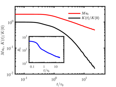
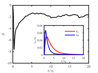
Figure 1: (a) Evolution of the turbulent Mach number $M_{t}$, the turbulence kinetic energy normalized with its initial value $K(t)/K(0)$, and the Reynolds number $R_{\lambda}$ (shown in inset). (b) The evolution of the skewness of the longitudinal velocity derivative $S$. The inset shows the energy dissipation rates: the solenoidal part $\varepsilon_{s}$ and the dilational part $\varepsilon_{d}$.

We now discuss the structure of the velocity gradient correlations in this flow. Figure 2 shows the evolution of the l.h.s. and r.h.s. of Eq. (2) and (3), the identities for the invariants of $\mathbf{A}^{(2)}$ and $\mathbf{A}^{(3)}$, respectively. The ratios between the two sides of those equations, shown in the insets, are exactly 1, as predicted for homogeneous flows.

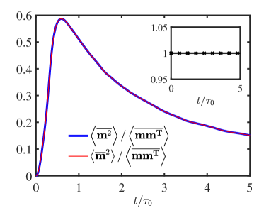
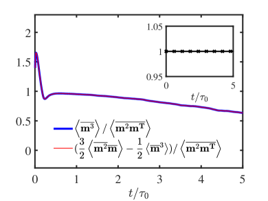
Figure 2: Evolution of invariants of $\mathbf{A}^{(2)}$ and $\mathbf{A}^{(3)}$ in compressible homogeneous isotropic decaying turbulence. (a) Second-order invariants, $\langle\overline{\mathbf{m}^{2}}\rangle/\langle\overline{\mathbf{mm^{T}}}\rangle$ and $\langle\overline{\mathbf{m}}^{2}\rangle/\langle\overline{\mathbf{mm^{T}}}\rangle$, the inset plots the ratio $\langle\overline{\mathbf{m}}^{2}\rangle/\langle\overline{\mathbf{m}^{2}}\rangle$. (b) Third-order invariants $\langle\overline{\mathbf{m}^{3}}\rangle/\langle\overline{\mathbf{m}^{2}\mathbf{m^{T}}}\rangle$ and $(\frac{3}{2}\langle\overline{\mathbf{m}^{2}}\overline{\mathbf{m}}\rangle-\frac{1}{2}\langle\overline{\mathbf{m}}^{3}\rangle)/\langle\overline{\mathbf{m}^{2}\mathbf{m^{T}}}\rangle$, the inset plots the ratio $\langle\overline{\mathbf{m}^{3}}\rangle/(\frac{3}{2}\langle\overline{\mathbf{m}^{2}}\overline{\mathbf{m}}\rangle-\frac{1}{2}\langle\overline{\mathbf{m}}^{3}\rangle)$.

Our analysis predicts, for homogeneous and isotropic turbulence, further relations among the components of $\mathbf{A}^{(2)}$ and $\mathbf{A}^{(3)}$. Figure 3a shows that $A^{(2)}_{1122}$ and $A^{(2)}_{1221}$ are equal during the entire simulation, as predicted by Eq. (7). In Fig. 3b, the ratio of the components $A^{(2)}_{1212}/A^{(2)}_{1111}$ also lies within $1/3$ and $2$ as predicted. It starts at $2$ since the flow is initially solenoidal. The rapid drop to values lower than $1$ is concurrent with the rise of dilational dissipation $\varepsilon_{d}$. The minimal possible value of $1/3$ for $A^{(2)}_{1212}/A^{(2)}_{1111}$ corresponds to a compressible irrotational flow. The observed value of $A^{(2)}_{1212}/A^{(2)}_{1111}$, close to $1.5$ at later times, indicates instead the prevalence of the solenoidal part.

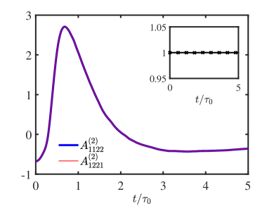
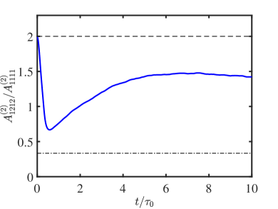
Figure 3: (a) Time evolution of $A^{(2)}_{1122}$ and $A^{(2)}_{1221}$ and their ratio (shown in inset).

Figure 4a shows the evolution of the invariants of $\mathbf{A}^{(3)}$ after the early stage when the flow rapidly adjusts in response to the initial divergence-free condition. Remarkably, the magnitude of $\langle\overline{\mathbf{w}^{2}}\overline{\mathbf{m}}\rangle$ is very small compared with the others, consistent with the observation that in compressible homogeneous turbulence, vorticity and dilation are nearly uncorrelated (Erlebacher & Sarkar, 1993; Wang et al., 2012). This, in view of Eq. (19), provides an additional relation: $3a_{2}\approx 3a_{3}+2a_{4}-2a_{5}$, which then leaves only 3 independent quantities for a complete determination of $\mathbf{A}^{(3)}$. Plugging Eq. (15) to (18) into this relation leads to

$$\frac{7}{6}A_{111111}\approx\frac{9}{2}A_{121211}+A_{111122}+A_{113232}.$$ (21)

Figure 4b This result may be helpful to reconstruct the complete isotropic expression of $A^{(3)}_{ipjqkr}$ from planar PIV or 2C LDV data, instead of requiring stereo-PIV or 3C LDV.

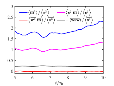
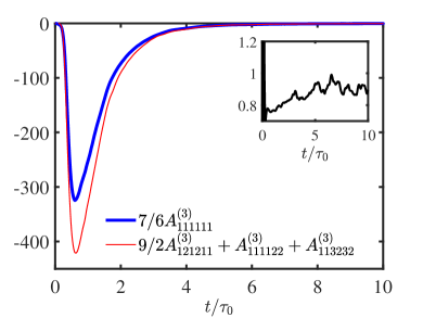
Figure 4: (a) Evolution of the invariants $\langle\overline{\mathbf{m}^{3}}\rangle$, $\langle\overline{\mathbf{w}^{2}}~{}\overline{\mathbf{m}}\rangle$, $\langle\overline{\mathbf{s}^{2}}~{}\overline{\mathbf{m}}\rangle$, and $\langle\overline{\mathbf{wsw}}\rangle$, all normalized by $\langle\overline{\mathbf{s}^{3}}\rangle$. (b) The values of the l.h.s. and r.h.s. of Eq. (21) and their ratio (shown in inset).

Next we perform a DNS of a planar compressible mixing layer, formed by two co-moving free streams with Mach numbers $Ma_{1}=U_{1}/c_{1}=7.5$ and $Ma_{2}=U_{2}/c_{2}=1.5$, respectively, in which $U_{1}$ and $U_{2}$ are the mean velocities in the upper and lower free streams, and $c_{1}$ and $c_{2}$ are the speeds of sound in the two streams. Similar with the setup of  Li & Jaberi (2011), at the inflow plane $x=0$, the mean stream velocity profile $U(0,y,z)$ is specified to be $U(0,y,z)=\frac{1}{2}\left[U_{1}+U_{2}+(U_{1}-U_{2})\tanh\left(2y/\delta_{\omega 0}\right)\right],$ with the inflow vorticity thickness ${\delta_{\omega 0}}=1$. The convective Mach number is $Ma_{c}=(U_{1}-U_{2})/(c_{1}+c_{2})=3$ and the Reynolds number is $Re_{c}=\rho_{1}(U_{1}-U_{2}){\delta_{\omega 0}}/\mu_{1}=3500$. The mean temperature profile at the inlet is given by the Crocco-Busemann law with a uniform mean pressure. The effective size of the computational domain is $450{\delta_{\omega 0}}\times 100{\delta_{\omega 0}}\times 16{\delta_{\omega 0}}$ in the $x$, $y$ and $z$ directions, respectively. The domain is discretized using a mesh of $3050\times 400\times 128$ nodes uniformly distributed in the $x$ and $z$ directions and stretched in the $y$ direction with higher resolution in the centre of the mixing layer. Near the outflow plane, a sponge layer with a highly stretched mesh is added to damp fluctuations near the boundary. Random velocity fluctuations are superposed on the mean profile at the inlet plane to trigger turbulence, which develops downstream, forming a large number of shocklets in both upper and lower parts of the mixing layer. When it is not too close to the inlet plane, the momentum thickness, $\theta$, grows linearly downstream and the mean velocity profiles are self-similar, i.e., $U(x,y)$ at different $x$ locations collapse to $U(\xi)$ with $\xi=(y-y_{c})/\theta$, where $y_{c}$ is the centre of the mixing layer. The result is validated by checking the balance of turbulence kinetic energy budget (not shown).

Figure 5 shows the ratio between the l.h.s. and the r.h.s. of Eq. (2) and (3) in the center region of the mixing layer $(-6\leqslant y/\theta\leqslant 6)$ at the downstream locations $x\delta_{\omega 0}=350$ (dashed lines) and $x/\delta_{\omega 0}=400$ (solid lines). Although the flow is not homogeneous, the ratios $\langle\overline{\mathbf{m}}^{2}\rangle/\langle\overline{\mathbf{m}^{2}}\rangle$ and $\langle\overline{\mathbf{m}^{3}}\rangle/(\frac{3}{2}\langle\overline{\mathbf{m}^{2}}\overline{\mathbf{m}}\rangle-\frac{1}{2}\langle\overline{\mathbf{m}}^{3}\rangle)$ are very close to unity, so Eqs. (2) and (3) are still approximately valid. Fig. 6 shows the profiles of various third-order invariants $\langle\overline{\mathbf{m}}^{3}\rangle$, $\langle\overline{\mathbf{w}^{2}}\overline{\mathbf{m}}\rangle$, $\langle\overline{\mathbf{s}^{2}}\overline{\mathbf{m}}\rangle$, $\langle\overline{\mathbf{s}^{3}}\rangle$ and $\langle\overline{\mathbf{wsw}}\rangle$. Despite the inhomogeneity and anisotropy, the vorticity-dilation correlation $\langle\overline{\mathbf{w}^{2}}\overline{\mathbf{m}}\rangle$ remains very small compared to other invariants, which could help to obtain more relations among invariants.

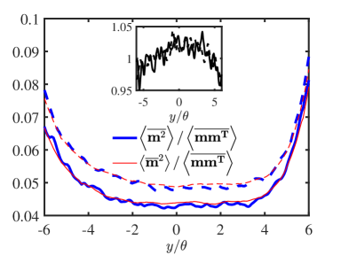
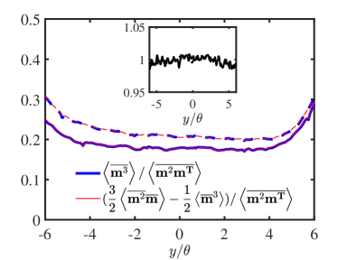
Figure 5: Approximate validity of the homogeneous relations in the compressible mixing layer. (a) Normalized second-order invariants, $\langle\overline{\mathbf{m}^{2}}\rangle/\langle\overline{\mathbf{mm^{T}}}\rangle$, $\langle\overline{\mathbf{m}}^{2}\rangle/\langle\overline{\mathbf{mm^{T}}}\rangle$, and their ratio (shown in the inset). (b) Normalized third-order invariants, $\langle\overline{\mathbf{m}^{3}}\rangle/\langle\overline{\mathbf{m}^{2}\mathbf{m^{T}}}\rangle$, $(\frac{3}{2}\langle\overline{\mathbf{m}^{2}}\overline{\mathbf{m}}\rangle-\frac{1}{2}\langle\overline{\mathbf{m}}^{3}\rangle)/\langle\overline{\mathbf{m}^{2}\mathbf{m^{T}}}\rangle$, and their ratio (shown in the inset). In both plots, dashed lines correspond to $x/\delta_{\omega 0}=350$ and solid lines to $x/\delta_{\omega 0}=400$.

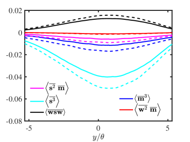
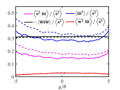
Figure 6: (a) Profiles of the invariants $\langle\overline{\mathbf{m}}^{3}\rangle$, $\langle\overline{\mathbf{w}^{2}}\overline{\mathbf{m}}\rangle$, $\langle\overline{\mathbf{s}^{2}}\overline{\mathbf{m}}\rangle$, $\langle\overline{\mathbf{s}^{3}}\rangle$ and $\langle\overline{\mathbf{wsw}}\rangle$ in the mixing layer. (b) Relative ratios $\langle\overline{\mathbf{m}^{3}}\rangle$/$\langle\overline{\mathbf{s}^{3}}\rangle$, $\langle\overline{\mathbf{w}^{2}}\overline{\mathbf{m}}\rangle$/$\langle\overline{\mathbf{s}^{3}}\rangle$, $\langle\overline{\mathbf{s}^{2}}\overline{\mathbf{m}}\rangle$/$\langle\overline{\mathbf{s}^{3}}\rangle$, and $\langle\overline{\mathbf{wsw}}\rangle$/$\langle\overline{\mathbf{s}^{3}}\rangle$. In both plots, dashed lines correspond to $x/\delta_{\omega 0}=350$ and solid lines to $x/\delta_{\omega 0}=400$.

4 Concluding Remarks

In summary, we derived exact relations among invariants of the moments of velocity gradients in compressible homogeneous turbulence and verified these relations by DNS of decaying compressible turbulence. Interestingly, these relations, derived under homogeneity assumptions, hold approximately in a compressible mixing layer. We also devised approaches to determine the full tensor with a minimal set of measurements in experiments. These relations could help, e.g., to determine separately the solenoidal and the dilational energy dissipation rates from only two velocity derivatives $\frac{\partial u_{1}}{\partial x_{1}}$ and $\frac{\partial u_{2}}{\partial x_{1}}$. In the future, it would be interesting to investigate the structure of the velocity gradient implied by these relations, as done by Betchov (1956) for incompressible turbulence.

Appendix

For vector gradients $\frac{\partial a_{i}}{\partial x_{j}}$, $\frac{\partial b_{i}}{\partial x_{j}}$ and $\frac{\partial c_{i}}{\partial x_{j}}$, we have, by elementary algebra:

$$\left\langle\frac{\partial a_{i}}{\partial x_{j}}\frac{\partial b_{j}}{\partial x_{k}}\frac{\partial c_{k}}{\partial x_{i}}\right\rangle =\frac{\partial}{\partial x_{j}}\left\langle a_{i}\frac{\partial b_{j}}{\partial x_{k}}\frac{\partial c_{k}}{\partial x_{i}}\right\rangle-\left\langle a_{i}\frac{\partial^{2}b_{j}}{\partial x_{j}\partial x_{k}}\frac{\partial c_{k}}{\partial x_{i}}\right\rangle-\left\langle a_{i}\frac{\partial b_{j}}{\partial x_{k}}\frac{\partial^{2}c_{k}}{\partial x_{i}\partial x_{j}}\right\rangle$$ (22)

$$\left\langle a_{i}\frac{\partial^{2}b_{j}}{\partial x_{j}\partial x_{k}}\frac{\partial c_{k}}{\partial x_{i}}\right\rangle =\frac{\partial}{\partial x_{k}}\left\langle a_{i}\frac{\partial b_{j}}{\partial x_{j}}\frac{\partial c_{k}}{\partial x_{i}}\right\rangle-\left\langle\frac{\partial a_{i}}{\partial x_{k}}\frac{\partial b_{j}}{\partial x_{j}}\frac{\partial c_{k}}{\partial x_{i}}\right\rangle-\left\langle a_{i}\frac{\partial b_{j}}{\partial x_{j}}\frac{\partial^{2}c_{k}}{\partial x_{k}\partial x_{i}}\right\rangle$$ (23)

$$\left\langle a_{i}\frac{\partial b_{j}}{\partial x_{k}}\frac{\partial^{2}c_{k}}{\partial x_{i}\partial x_{j}}\right\rangle =\frac{\partial}{\partial x_{i}}\left\langle a_{i}\frac{\partial b_{j}}{\partial x_{k}}\frac{\partial c_{k}}{\partial x_{j}}\right\rangle-\left\langle\frac{\partial a_{i}}{\partial x_{i}}\frac{\partial b_{j}}{\partial x_{k}}\frac{\partial c_{k}}{\partial x_{j}}\right\rangle-\left\langle a_{i}\frac{\partial^{2}b_{j}}{\partial x_{i}\partial x_{k}}\frac{\partial c_{k}}{\partial x_{j}}\right\rangle$$ (24)

$$\left\langle a_{i}\frac{\partial^{2}b_{j}}{\partial x_{i}\partial x_{k}}\frac{\partial c_{k}}{\partial x_{j}}\right\rangle =\frac{\partial}{\partial x_{k}}\left\langle a_{i}\frac{\partial b_{j}}{\partial x_{i}}\frac{\partial c_{k}}{\partial x_{j}}\right\rangle-\left\langle\frac{\partial a_{i}}{\partial x_{k}}\frac{\partial b_{j}}{\partial x_{i}}\frac{\partial c_{k}}{\partial x_{j}}\right\rangle-\left\langle a_{i}\frac{\partial b_{j}}{\partial x_{i}}\frac{\partial^{2}c_{k}}{\partial x_{k}\partial x_{j}}\right\rangle$$ (25)

$$\left\langle a_{i}\frac{\partial b_{j}}{\partial x_{j}}\frac{\partial^{2}c_{k}}{\partial x_{k}\partial x_{i}}\right\rangle =\frac{\partial}{\partial x_{i}}\left\langle a_{i}\frac{\partial b_{j}}{\partial x_{j}}\frac{\partial c_{k}}{\partial x_{k}}\right\rangle-\left\langle\frac{\partial a_{i}}{\partial x_{i}}\frac{\partial b_{j}}{\partial x_{j}}\frac{\partial c_{k}}{\partial x_{k}}\right\rangle-\left\langle a_{i}\frac{\partial^{2}b_{j}}{\partial x_{i}\partial x_{j}}\frac{\partial c_{k}}{\partial x_{k}}\right\rangle$$ (26)

$$\left\langle a_{i}\frac{\partial b_{j}}{\partial x_{i}}\frac{\partial^{2}c_{k}}{\partial x_{k}\partial x_{j}}\right\rangle =\frac{\partial}{\partial x_{j}}\left\langle a_{i}\frac{\partial b_{j}}{\partial x_{i}}\frac{\partial c_{k}}{\partial x_{k}}\right\rangle-\left\langle\frac{\partial a_{i}}{\partial x_{j}}\frac{\partial b_{j}}{\partial x_{i}}\frac{\partial c_{k}}{\partial x_{k}}\right\rangle-\left\langle a_{i}\frac{\partial^{2}b_{j}}{\partial x_{i}\partial x_{j}}\frac{\partial c_{k}}{\partial x_{k}}\right\rangle\,.$$ (27)

Multiplying (23), (24) and (27) by $-1$, and summing over, one obtains:

$$2\langle\overline{\mathbf{h^{a}}\mathbf{h^{b}}\mathbf{h^{c}}}\rangle=\langle\overline{\mathbf{h^{a}}\mathbf{h^{b}}}\,\overline{\mathbf{h^{c}}}\rangle+\langle\overline{\mathbf{h^{b}}\mathbf{h^{c}}}\,\overline{\mathbf{h^{a}}}\rangle+\langle\overline{\mathbf{h^{c}}\mathbf{h^{a}}}\,\overline{\mathbf{h^{b}}}\rangle-\langle\overline{\mathbf{h^{a}}}\,\overline{\mathbf{h^{b}}}\,\overline{\mathbf{h^{c}}}\rangle,$$ (28)

in which $\mathbf{h^{a}}=\nabla\mathbf{a}$ etc. For divergence-free fields, this yields $\langle\overline{\nabla\mathbf{a}\nabla\mathbf{b}\nabla\mathbf{c}}\rangle=0$. An equivalent form of this special case has been shown in Appendix D of Eyink (2006).

References

- Betchov (1956) Betchov, R. 1956 An inequality concerning the production of vorticity in isotropic turbulence. J. Fluid Mech. 1, 497–504.
- Bradshaw & Perot (1993) Bradshaw, P. & Perot, J. B. 1993 A note on turbulent energy dissipation in the viscous wall region. Phys. Fluids A 5, 3305–3306.
- Buaria et al. (2020) Buaria, D., Pumir, A. & Bodenschatz, E. 2020 Vortex stretching and enstrophy production in high Reynolds number turbulence. Phys. Rev. Fluids 5, 104602.
- Chen et al. (2019) Chen, S., Wang, J., Li, H., Wan, M. & Chen, S. 2019 Effect of compressibility on small scale statistics in homogeneous shear turbulence. Phys. Fluids 31, 025107.
- Chu et al. (2014) Chu, Y. B., Wang, L. & Lu, X. Y. 2014 Interaction between strain and vorticity in compressible turbulent boundary layer. Sci. China Phys., Mech. Astron. 57, 2316–2329.
- Erlebacher & Sarkar (1993) Erlebacher, G. & Sarkar, S. 1993 Rate of strain tensor statistics in compressible homogeneous turbulence. Phys. Fluids A 5, 3240–3254.
- Eyink (2006) Eyink, G. 2006 Multi-scale gradient expansion of the turbulent stress tensor. J. Fluid Mech. 549, 159–190.
- Fang et al. (2019) Fang, J., Gao, F., Moulinec, C. & Emerson, D. R. 2019 An improved parallel compact scheme for domain-decoupled simulation of turbulence. Int. J. for Numer. Meth. Fl. 90 (10), 479–500.
- Fang et al. (2013) Fang, J., Li, Z. & Lu, L. 2013 An optimized low-dissipation monotonicity-preserving scheme for numerical simulations of high-speed turbulent flows. J. Sci. Comput. 56, 67–95.
- Fang et al. (2014) Fang, J., Yao, Y., Li, Z. & Lu, L. 2014 Investigation of low-dissipation monotonicity-preserving scheme for direct numerical simulation of compressible turbulent flows. Comput. Fluids 104, 55–72.
- Fang et al. (2015) Fang, J., Yao, Y., Zheltovodov, A. A., Li, Z. & Lu, L. 2015 Direct numerical simulation of supersonic turbulent flows around a tandem expansion-compression corner. Phys. Fluids 12 (27).
- Fang et al. (2020) Fang, J., Zheltovodov, A. A., Yao, Y., Moulinec, C. & Emerson, D. R. 2020 On the turbulence amplification in shock-wave/turbulent boundary layer interaction. J. Fluid Mech. 897, A32.
- Fang et al. (2016) Fang, L., Zhang, Y. J., Fang, J. & Zhu, Y. 2016 Relation of the fourth-order statistical invariants of velocity gradient tensor in isotropic turbulence. Phys. Rev. E 94, 023114.
- Frisch (1995) Frisch, U. 1995 Turbulence: The legacy of A. N. Kolmogorov. Cambridge Univ. Press.
- Gottlieb & Shu (1998) Gottlieb, S. & Shu, C. W. 1998 Total variation diminishing runge-kutta schemes. Math. Comput. 67, 73–85.
- Lele (1992) Lele, Sanjiva K. 1992 Compact finite difference schemes with spectral-like resolution. J. Comput. Phys. 103, 16–42.
- Li & Jaberi (2011) Li, Z. & Jaberi, F. A. 2011 A high-order finite difference method for numerical simulations of supersonic turbulent flows. J. Numer. Meth. Fluids 68 (6), 740–766.
- Ma & Xiao (2016) Ma, Z. & Xiao, Z. 2016 Turbulent kinetic energy production and flow structures in compressible homogeneous shear flow. Phys. Fluids 28, 096102.
- Meneveau (2011) Meneveau, C. 2011 Lagrangian dynamics and models of the velocity gradient tensor in turbulent flows. Annu. Rev. Fluid Mech. 43, 219–245.
- Pan & Johnsen (2017) Pan, S. & Johnsen, E. 2017 The role of bulk viscosity on the decay of compressible homogeneous, isotropic turbulence. J. Fluid Mech. 833, 717–744.
- Pirozzoli & Grasso (2004) Pirozzoli, S. & Grasso, F. 2004 Direct numerical simulations of isotropic compressible turbulence: Influence of compressibility on dynamics and structures. Phys. Fluids 16, 4386–4407.
- Pope (2000) Pope, S. B. 2000 Turbulent flows. Cambridge University Press.
- Pumir (2017) Pumir, A. 2017 Structure of the velocity gradient tensor in turbulent shear flows. Phys. Rev. Fluids 2 (7), 074602.
- Pumir et al. (2016) Pumir, A., Xu, H. & Siggia, E. D. 2016 Small-scale anisotropy in turbulent boundary layers. J. Fluid Mech. 804, 5–23.
- Samtaney et al. (2001) Samtaney, R., Pullin, D. I. & Kosovic, B. 2001 Direct numerical simulation of decaying compressible turbulence and shocklet statistics. Phys. Fluids 13 (5), 1415–1430.
- Sreenivasan & Antonia (1997) Sreenivasan, K. R. & Antonia, R. A. 1997 The phenomenology of small-scale turbulence. Annu. Rev. Fluid Mech. 29, 435–472.
- Suman & Girimaji (2009) Suman, S. & Girimaji, S. S. 2009 Homogenized Euler equation: a model for compressible velocity gradient dynamics. J. Fluid Mech. 620, 177–194.
- Suman & Girimaji (2011) Suman, S. & Girimaji, S. S. 2011 Dynamical model for velocity-gradient evolution in compressible turbulence. J. Fluid Mech. 683, 289–319.
- Suman & Girimaji (2013) Suman, S. & Girimaji, S. S. 2013 Velocity gradient dynamics in compressible turbulence: Characterization of pressure-Hessian tensor. Phys. Fluids 25, 125103.
- Tsinober (2009) Tsinober, A. 2009 An Informal Conceptual Introduction to Turbulence. Springer.
- Vaghel & Madnia (2015) Vaghel, N.S. & Madnia, C.K. 2015 Local flow topology and velocity gradient invariants in compressible turbulent mixing layer. J. Fluid Mech. 774, 67–94.
- Vreman & Kuerten (2014) Vreman, A. W. & Kuerten, J. G. M. 2014 Statistics of spatial derivatives of velocity and pressure in turbulent channel flows. Phys. Fluids 26, 085103.
- Wang et al. (2012) Wang, J., Shi, Y., Wang, L.-P., Xiao, Z., He, X. T. & Chen, S. 2012 Effect of compressibility on the small-scale structures in isotropic turbulence. J. Fluid Mech. 713, 588–631.
- Wang et al. (2018) Wang, J., Wan, M., Chen, S., Xie, C. & Chen, S. 2018 Effect of shock waves on the statistics and scaling in compressible isotropic turbulence. Phys. Rev. E 97, 043108.
- Yang et al. (2020) Yang, P.-F., Pumir, A. & Xu, H. 2020 Dynamics and invariants of the perceived velocity gradient tensor in homogeneous and isotropic turbulence. J. Fluid Mech. 897, A9.