Interactive fixed effects are a popular means to model unobserved heterogeneity in panel data. Models with interactive fixed effects are well studied in the low-dimensional case where the number of parameters to be estimated is small. However, they are largely unexplored in the high-dimensional case where the number of parameters is large, potentially much larger than the sample size itself. In this paper, we develop new econometric methods for the estimation of high-dimensional panel data models with interactive fixed effects. Our estimator is based on similar ideas as the very popular common correlated effects (CCE) estimator which is frequently used in the low-dimensional case. We thus call our estimator a high-dimensional CCE estimator. We derive theory for the estimator both in the large-$T$-case, where the time series length $T$ tends to infinity, and in the small-$T$-case, where $T$ is a fixed natural number. The theoretical analysis of the paper is complemented by a simulation study which evaluates the finite sample performance of the estimator.

Key words: panel data; interactive fixed effects; CCE estimator; high-dimensional model; lasso.

JEL classifications: C13; C23; C55.

1 Introduction

A very popular and widely used framework in panel data econometrics are models with interactive fixed effects. In its simplest form, the model is given by the equation

$$Y_{it}=\beta^{\top}X_{it}+\gamma_{i}^{\top}F_{t}+\varepsilon_{it}$$ (1.1)

for $1\leq t\leq T$ and $1\leq i\leq n$, where $i$ is the cross-section index and $t$ the time series index, $Y_{it}$ is a real-valued response variable, $X_{it}$ is a vector of $p$ regressors and $\beta$ is the unknown parameter vector of length $p$. The error structure of the model comprises two components: a standard idiosyncratic error term $\varepsilon_{it}$ and the interactive fixed effects component $\gamma_{i}^{\top}F_{t}$, where $F_{t}$ is a vector of unobserved factors and $\gamma_{i}$ is a vector of unobserved factor loadings. The regressors $X_{it}$ are allowed to be correlated with the factors $F_{t}$ and the loadings $\gamma_{i}$, which induces endogeneity issues in model (1.1). The interactive fixed effects in (1.1) allow to model unobserved heterogeneity in a quite flexible manner, in particular, much more flexibly than standard fixed effects $a_{i}$ and $b_{t}$ in a model of the form $Y_{it}=\beta^{\top}X_{it}+a_{i}+b_{t}+\varepsilon_{it}$.

In recent years, ever larger economic panel data sets have been collected, with many of them being high-dimensional in the following sense: the number of available explanatory variables $p$ is very large, potentially even larger than the sample size $nT$ itself. To deal with such high-dimensional data structures, new econometric methods are required. In this paper, we study a high-dimensional version of the panel model (1.1) with interactive fixed effects. Our main contribution is to develop a novel estimator of the high-dimensional parameter vector $\beta$ in this model and to derive theory for it. The idea behind the estimator is to eliminate the unobserved factors by transforming the model. More specifically, we apply a particular projection matrix to the model equation which (approximately) eliminates the factors. Hence, our approach is based on the same philosophy as the common correlated effects (CCE) method of Pesaran (2006): we “project away” the unobserved factors. We thus call our estimator a high-dimensional CCE estimator. Nevertheless, it is markedly different from the original CCE estimator. The main reason is that in the high-dimensional case, it is much more difficult to “project away” the factors. To achieve this, a completely new approach to construct the projection matrix is required.

In the traditional low-dimensional case where the number of regressors $p$ is small and fixed, model (1.1) has been analyzed extensively in the literature. Presumably the most popular estimator of $\beta$ in this traditional setting is the CCE estimator of Pesaran (2006). We will come back to this estimator in Section 4, where we discuss it in detail. Since its introduction, the CCE estimator has become a standard tool in panel data econometrics, giving rise to a whole new strand of the literature with numerous extensions such as Kapetanios et al. (2011), Chudik et al. (2011), Pesaran and Tosetti (2011), Chudik and Pesaran (2015), Westerlund (2018), Westerlund et al. (2019), Juodis et al. (2021) and Juodis (2021) to name just a few.

There are several alternatives to the CCE estimator which can be used to estimate $\beta$ in the low-dimensional case. The most important one is a least squares approach which simultaneously estimates the target vector $\beta$ and the factor structure consisting of the vectors $\gamma_{i}$ and $F_{t}$. This approach was originally studied in Bai (2009) and theoretically further explored in Moon and Weidner (2015) among others. The philosophy behind this approach is quite different from that of the CCE method: rather than eliminating the factors and the corresponding loadings, these are estimated as additional parameters. One disadvantage of this least squares approach is that the criterion function to be minimized is not convex. Hence, to compute the estimator, one needs to solve a non-convex optimization problem. Recently, least squares estimation with nuclear norm penalization has been proposed to overcome this problem. The resulting estimator minimizes a convex criterion function and can thus be efficiently computed by standard methods from convex optimization. It has, however, the disadvantage that its convergence rate is fairly slow in general. Recent studies on nuclear norm penalized estimators for panel data models with interactive fixed effects include Chernozhukov et al. (2018), Beyhum and Gautier (2019) and Moon and Weidner (2019).

Whereas panel models with interactive fixed effects are well studied in the low-dimensional case, they are largely unexplored in high dimensions. Indeed, the literature on high-dimensional panels in general is quite limited. High-dimensional panel models with random and fixed effects have been considered in Kock (2013, 2016), Belloni et al. (2016) and Kock and Tang (2019): Kock (2013) derives theory for bridge estimators in both random and fixed effects models, while Kock (2016) analyzes a model with a hybrid error structure that is in-between random and fixed effects. Belloni et al. (2016) introduce the so-called cluster-lasso to estimate the unknown parameters in a model with an individual fixed effect. Finally, Kock and Tang (2019) use desparsified-lasso techniques to perform inference in a dynamic panel model with fixed effects. Econometric methods for high-dimensional panel models with interactive fixed effects have been developed in Lu and Su (2016) and Belloni et al. (2019): Lu and Su (2016) extend the least squares method of Bai (2009) to a high-dimensional dynamic panel model by adding a group-lasso penalty. However, they only consider a situation where $p$ grows fairly slowly with the sample size. Belloni et al. (2019) develop nuclear norm penalized estimation methods for high-dimensional quantile panel regression. A high-dimensional version of the panel partial factor model, which is closely related to panel models with interactive fixed effects, is investigated in Hansen and Liao (2019). Notably, none of the mentioned studies consider extensions of the popular and simple-to-implement CCE approach of Pesaran (2006). As discussed in more detail in Section 4, the reason is that the CCE approach breaks down in high dimensions and naive extensions to the high-dimensional case fail dramatically.

In this paper, we develop an estimator which can be regarded as a non-trivial extension of the CCE approach to high dimensions. We consider a high-dimensional version of the panel model with interactive fixed effects examined in Pesaran (2006). A detailed description of the model together with the technical assumptions imposed on the model components is provided in Section 2, while identification issues are discussed in Section 3. Our estimator is constructed step by step in Section 4. Its theoretical properties are analyzed in Section 5. Notably, in contrast to most of the literature on panel models with interactive fixed effects, we not only study the large-$T$-case where both $n$ and $T$ tend to infinity, but also derive theoretical results for the small-$T$-case where $n$ tends to infinity and $T$ is a fixed natural number. The methodological and theoretical analysis of the paper is complemented by a simulation study in Section 6. Our methods are implemented in the R package ccehd which can be downloaded at https://github.com/ChriWalsh/ccehd.

Notation. Matrices are denoted by bold letters, whereas scalars and vectors are printed in normal font. For a vector $x=(x_{1},\ldots,x_{q})^{\top}\in\mathbb{R}^{q}$ and a set $S\subseteq\{1,\ldots,q\}$, we let $x_{S}=(x_{i}:i\in S)$ be the vector which consists of the entries $x_{i}$ with $i\in S$ only. Moreover, $\|x\|=(\sum_{i}x_{i}^{2})^{1/2}$ is the Euclidean norm of $x$, $\|x\|_{1}=\sum_{i}|x_{1}|$ its $\ell_{1}$-norm, and $\|x\|_{\infty}=\max_{i}|x_{i}|$ its $\ell_{\infty}$-norm. The symbols $\psi_{\min}(\boldsymbol{A})$ and $\psi_{\max}(\boldsymbol{A})$ are used to denote the minimal and maximal eigenvalue of a square matrix $\boldsymbol{A}\in\mathbb{R}^{q\times q}$. In addition, we sometimes write $\psi_{1}(\boldsymbol{A})\geq\psi_{2}(\boldsymbol{A})\geq\ldots\geq\psi_{q}(\boldsymbol{A})$ to denote the eigenvalues of $\boldsymbol{A}$ (in decreasing order). For a general (not necessarily square) matrix $\boldsymbol{A}=(a_{ij})$, $\|\boldsymbol{A}\|$, $\|\boldsymbol{A}\|_{1}$, $\|\boldsymbol{A}\|_{\infty}$ and $\|\boldsymbol{A}\|_{\text{max}}$ are its spectral norm, $\ell_{1}$-norm, $\ell_{\infty}$-norm and elementwise norm, respectively. In particular, $\|\boldsymbol{A}\|=\psi_{\max}^{1/2}(\boldsymbol{A}^{\top}\boldsymbol{A})$, $\|\boldsymbol{A}\|_{1}=\max_{j}\sum_{i}|a_{ij}|$, $\|\boldsymbol{A}\|_{\infty}=\max_{i}\sum_{j}|a_{ij}|$ and $\|\boldsymbol{A}\|_{\max}=\max_{ij}|a_{ij}|$. The symbol $\boldsymbol{A}^{-}$ stands for the generalized inverse of a matrix $\boldsymbol{A}$ and the symbol $\boldsymbol{I}_{q}$ for the $q\times q$ identity matrix. Sometimes, we also write $\boldsymbol{I}$ instead of $\boldsymbol{I}_{q}$ for short. Finally, the indicator function is denoted by $1(\cdot)$ and the cardinality of a set $S$ by $|S|$.

2 Model framework

2.1 Data structure

We observe a sample of panel data $\{(Y_{it},X_{it}):1\leq t\leq T,\,1\leq i\leq n\}$ with real-valued random variables $Y_{it}$ and $\mathbb{R}^{p}$-valued random vectors $X_{it}=(X_{it,1},\ldots,X_{it,p})^{\top}$, where $n$ is the cross-section dimension and $T$ the time series length. The dimension $p$ of the random vector $X_{it}$ is allowed to be large, potentially much larger than the dimensions $n$ and $T$. We consider the following two scenarios:

1. the large-$T$-case where both $n\to\infty$ and $T\to\infty$

2. the small-$T$-case where $n\to\infty$ but $T$ is a fixed natural number.

Asymptotic statements are thus understood in the sense that $n\to\infty$ (and $T\to\infty$ in the large-$T$-case).

2.2 Model equations

We consider a high-dimensional version of the linear panel data model with interactive fixed effects analyzed in Pesaran (2006). The model has the form

$$Y_{it}=\beta^{\top}X_{it}+\gamma_{i}^{\top}F_{t}+\varepsilon_{it}\qquad(1\leq t\leq T,\,1\leq i\leq n),$$ (2.1)

where $\beta=(\beta_{1},\ldots,\beta_{p})^{\top}$ is the unknown parameter vector, $X_{it}$ is the vector of regressors, $\varepsilon_{it}$ is the idiosyncratic error component with $\mathbb{E}[\varepsilon_{it}]=0$ for all $i$ and $t$, and $\gamma_{i}^{\top}F_{t}$ is the interactive fixed effects part of the error. More specifically, $F_{t}=(F_{t,1},\ldots,F_{t,K})^{\top}$ is a $K$-dimensional vector of unobserved factors and $\gamma_{i}=(\gamma_{i,1},\ldots,\gamma_{i,K})^{\top}$ is a vector of (unknown) individual-specific factor loadings. The regressors in (2.1) are supposed to have the structure

$$X_{it}=\boldsymbol{\Gamma}_{i}F_{t}+Z_{it},$$ (2.2)

where $\boldsymbol{\Gamma}_{i}\in\mathbb{R}^{p\times K}$ is a matrix of individual-specific factor loadings and $Z_{it}$ is the idiosyncratic part of the regressors with $\mathbb{E}[Z_{it}]=0$ for all $i$ and $t$. This structure implies that the regressors $X_{it}$ are correlated with the error terms $e_{it}=\gamma_{i}^{\top}F_{t}+\varepsilon_{it}$ via the interactive fixed effects. In matrix notation, model (2.1)–(2.2) can be formulated as

$$Y_{i}=\boldsymbol{X}_{i}\beta+\boldsymbol{F}\gamma_{i}+\varepsilon_{i}\quad\text{with}\quad\boldsymbol{X}_{i}=\boldsymbol{F}\boldsymbol{\Gamma}_{i}^{\top}+\boldsymbol{Z}_{i}\qquad(1\leq i\leq n),$$ (2.3)

where $Y_{i}=(Y_{i1},\ldots,Y_{iT})^{\top}$, $\boldsymbol{X}_{i}=(X_{i1}\ldots X_{iT})^{\top}$, $\boldsymbol{F}=(F_{1}\ldots F_{T})^{\top}$, $\varepsilon_{i}=(\varepsilon_{i1},\ldots$ $\ldots,\varepsilon_{iT})^{\top}$ and $\boldsymbol{Z}_{i}=(Z_{i1}\ldots Z_{iT})^{\top}$. Following Pesaran (2006), one may additionally include observed factors in model (2.1)–(2.2) and allow for heterogeneous parameter vectors $\beta_{i}=\beta+\eta_{i}$ with i.i.d. disturbances $\eta_{i}$. For simplicity of exposition, however, we ignore these extensions in the sequel.

The main difference of model (2.1)–(2.2) from Pesaran’s original model is that the dimension $p$ of the regressors $X_{it}=(X_{it,1},\ldots,X_{it,p})^{\top}$ is large, possibly much larger than the overall sample size $nT$. Without structural constraints on the parameter vector $\beta$, model (2.1)–(2.2) is not estimable in general. As usual in the literature on high-dimensional statistics, we impose a sparsity constraint on $\beta$. In particular, we assume that the set $S=\{j:\beta_{j}\neq 0\}$ of non-zero components of $\beta$ has cardinality $s:=|S|$ considerably smaller than the sample size $nT$. Hence, only a small subset of regressors is active, that is, enters the model with a non-zero coefficient. Precise conditions on the size of the sparsity index $s$ are provided below.

In contrast to the number of regressors $p$, the number of unknown factors $K$ is assumed to be small as in Pesaran’s low-dimensional version of the model. Assuming that $K$ is comparably small makes sense as $K$ plays a role analogous to the number of active regressors $s$ rather than the total number of regressors $p$. In principle, it is possible to allow $K$ to grow slowly with the sample size. However, for simplicity of exposition, we assume throughout the paper that $K$ is a fixed natural number.

2.3 Assumptions

The components of model (2.1)–(2.2) are assumed to satisfy the following regularity conditions:

1. The factors $F_{t}$ are independent of the loadings $\gamma_{i}$ and $\boldsymbol{\Gamma}_{i}$, the idiosyncratic components of the regressors $Z_{it^{\prime}}$ and the idiosyncratic errors $\varepsilon_{it^{\prime}}$ for all $i$, $t$ and $t^{\prime}$. For all $t$ and $k$, it holds that $\mathbb{E}|F_{t,k}|^{\theta}\leq C<\infty$ for some $\theta>8$.

2. The factor loadings $\gamma_{i}$ and $\boldsymbol{\Gamma}_{i}$ are independent from $Z_{i^{\prime}t}$ and $\varepsilon_{i^{\prime}t}$ for all $i$, $i^{\prime}$ and $t$. Moreover, they are independent across $i$ with means $\gamma=\mathbb{E}[\gamma_{i}]$ and $\boldsymbol{\Gamma}=\mathbb{E}[\boldsymbol{\Gamma}_{i}]$ and uniformly bounded fourth moments.

3. The idiosyncratic errors $\varepsilon_{it}$ are independent from $Z_{i^{\prime}t^{\prime}}$ for all $i$, $i^{\prime}$, $t$ and $t^{\prime}$. Moreover, they are independent across $i$. For all $i$ and $t$, it holds that $\mathbb{E}[\varepsilon_{it}]=0$ and $\mathbb{E}|\varepsilon_{it}|^{\theta}\leq C<\infty$ for some $\theta>8$.

4. The variables $Z_{it}$ are independent across $i$. For all $i$, $j$ and $t$, it holds that $\mathbb{E}[Z_{it,j}]=0$ and $\mathbb{E}|Z_{it,j}|^{\theta}\leq C<\infty$ for some $\theta>8$.

The assumption in (M3) that $\varepsilon_{it}$ is independent from $Z_{i^{\prime}t^{\prime}}$ for all $i$, $i^{\prime}$, $t$ and $t^{\prime}$ is only for convenience. It can be replaced by the following weaker assumption at the cost of a more involved notation in the proofs: The idiosyncratic errors $\varepsilon_{it}$ have the form $\varepsilon_{it}=\nu(Z_{it})\eta_{it}$, where $\nu(\cdot)$ is a non-negative volatility function with $\sup_{z\in\mathbb{R}^{p}}\nu(z)\leq C<\infty$ and $\eta_{it}$ are random variables with zero mean and unit variance that are independent from $Z_{i^{\prime}t^{\prime}}$ for all $i$, $i^{\prime}$, $t$ and $t^{\prime}$. In the large-$T$-case, we assume in addition to (M1)–(M4) that the model variables form weakly dependent time series processes that satisfy the following mixing conditions:

1. Let $\alpha(m)$ be non-negative real numbers which decay exponentially fast to $0$ as $m\to\infty$, in particular, $\alpha(m)\leq Ca^{m}$ for some $0\leq a<1$ and $C>0$.

   1. For each $k$, the time series $\mathcal{F}_{k,T}=\{F_{t,k}:1\leq t\leq T\}$ is strongly mixing with mixing coefficients $\alpha_{k,T}^{F}(m)\leq\alpha(m)$.

   2. For each $i$, the time series $\mathcal{E}_{i,T}=\{\varepsilon_{it}:1\leq t\leq T\}$ is strongly mixing with mixing coefficients $\alpha_{i,T}^{\varepsilon}(m)\leq\alpha(m)$.

   3. For each $i$ and $j$, the time series $\mathcal{Z}_{ij,T}=\{Z_{it,j}:1\leq t\leq T\}$ is strongly mixing with mixing coefficients $\alpha_{ij,T}^{Z}(m)\leq\alpha(m)$.

Conditions (M1)–(M5) are very similar to the assumptions in Pesaran (2006). However, unlike there, we do not impose any linearity and stationarity assumptions on the involved time series. In particular, the factors need not be stationary. It is in principle possible to drop assumption (M5) in the large-$T$-case and to do without any conditions on the time series dependence of the model variables as in the small-$T$-case. However, then we could not fully account for the time series information in the data. As a consequence, we would obtain a slower convergence rate for our estimator of the parameter vector $\beta$. For simplicity, the mixing coefficients in (M5) are assumed to decay to zero exponentially fast. It is possible though to allow for sufficiently fast polynomial decay instead.

In order to construct a consistent estimator of the parameter vector $\beta$, we have to make sure that the dimension $p$ is not too large and the true parameter vector $\beta$ is sufficiently sparse. Besides (M1)–(M5), we thus need some restrictions on the dimension $p$ and the sparsity index $s$.

In the large-$T$-case, we impose the following conditions on the dimension parameters $n$, $T$, $p$, $s$ and $K$ in the model:

1. The dimensions $n$, $T$ and $p$ are such that $n^{(\theta/2)-1}/T\gg p$ and $T^{(\theta/2)-1}/n\gg p$, where $a_{n,p,T}\gg b_{n,p,T}$ means that $b_{n,p,T}/a_{n,p,T}\leq C(npT)^{-\xi}$ for some small $\xi>0$ and $\theta$ is specified in (M1), (M3) and (M4).

2. The set $S=\{j:\beta_{j}\neq 0\}$ of non-zero components of $\beta$ has cardinality $s:=|S|$ with $s=o(\min\{n,T\}/\log(npT))$.

3. The number of factors $K$ is a fixed natural number with $K<T$ and $K\leq p$.

(D_ℓ1) essentially says that $p$ is not allowed to grow too quickly in comparison to $n$ and $T$. To better understand the restrictions on $p$, let us consider the special case $n=T$. In this case, the two restrictions of (D_ℓ1) simplify to $(nT)^{(\theta/4)-1}\gg p$. Hence, how fast $p$ can grow in comparison to the sample size $nT$ depends on how many moments $\theta$ the model variables $F_{t}$, $Z_{it}$ and $\varepsilon_{it}$ have. If all moments exist, $\theta$ can be chosen as large as desired and $p$ can grow as any polynomial of $nT$. If $\theta$ is quite small in contrast, say $\theta=8+\delta$ for some small $\delta>0$, then $p$ can only grow slightly faster than the sample size $nT$. (D_ℓ2) imposes constraints on the growth of the sparsity index $s$, that is, on the number of non-zero components of $\beta$. As one can see, $s$ is restricted to grow slightly more slowly than $\min\{n,T\}$. In the special case $n=T$, in particular, $s$ can only grow slightly more slowly than $\sqrt{nT}$.

In the small-$T$-case, our conditions on the dimension parameters $n$, $T$, $p$, $s$ and $K$ are as follows:

1. The dimensions $n$ and $p$ are such that $n^{(\theta/4)-1}\gg p$, where $a_{n,p}\gg b_{n,p}$ means that $b_{n,p}/a_{n,p}\leq C(np)^{-\xi}$ for some small $\xi>0$ and $\theta$ is specified in (M1), (M3) and (M4).

2. The set $S=\{j:\beta_{j}\neq 0\}$ of non-zero components of $\beta$ has cardinality $s:=|S|$ with $s=o((np)^{-2/\theta}\sqrt{n/\log p})$.

3. The number of factors $K$ is a fixed natural number with $K<T$ and $K\leq p$.

(D_s1) puts restrictions on the growth of $p$. Analogously to the large-$T$-case, the more moments $\theta$ exist, the faster $p$ is allowed to grow in comparison to $n$. In particular, if all moments exist, then $p$ can grow as any polynomial of $n$. (D_s2) imposes constraints on the growth of the sparsity index $s$. As can be seen, the more moments $\theta$ exist, the faster $s$ is allowed to increase. In particular, if all moments exist, then $s$ can grow almost as fast as $\sqrt{n}$. In contrast, if only a few moments exist, say $\theta=8+\delta$ for some small $\delta>0$, then $s$ must grow considerably more slowly than $\sqrt{n}$.

3 Identification

Model (2.3) contains the following unobserved components: the parameter vector $\beta$, the factor structure $\Theta_{\text{fac}}=\{\boldsymbol{F},\{\gamma_{i},\boldsymbol{\Gamma}_{i}\}_{i=1}^{n}\}$ consisting of the factors and their loadings, and the idiosyncratic structure $\Theta_{\text{idio}}=\{\boldsymbol{Z}_{i},\varepsilon_{i}\}_{i=1}^{n}$ consisting of the idiosyncratic part of the regressors and the idiosyncratic errors. Importantly, the parameter vector $\beta$, the factor structure $\Theta_{\text{fac}}$ and the idiosyncratic structure $\Theta_{\text{idio}}$ are in general not identified. Put differently, the parameter vector $\beta$, the factor structure $\Theta_{\text{fac}}$ and the idiosyncratic structure $\Theta_{\text{idio}}$ which satisfy the model equations in (2.3) and the assumptions of Section 2.3 are in general not unique.

In what follows, we show that the parameter vector $\beta$ and the number of factors $K$ are identified if certain additional constraints are imposed. That the factor structure $\Theta_{\text{fac}}$ (apart from $K$) and the idiosyncratic structure $\Theta_{\text{idio}}$ remain unidentified is no problem at all for our methods and theory. For our theoretical arguments to work, it suffices to consider some factor structure $\Theta_{\text{fac}}$ and some idiosyncratic structure $\Theta_{\text{idio}}$ such that the model equations and the technical conditions are fulfilled. Which version is considered does not matter. Since we work with different identification constraints in the large-$T$ and the small-$T$-case, we discuss these two cases separately.

3.1 Identification in the large-$\boldsymbol{T}$-case

In order to identify the number of factors $K$, we impose the following condition on the factors $F_{t}$:

1. It holds that

   $$\Big{\|}\mathbb{E}\Big{[}\frac{1}{T}\sum_{t=1}^{T}F_{t}F_{t}^{\top}\Big{]}-\boldsymbol{\Omega}\Big{\|}=O\Big{(}\frac{1}{\sqrt{T}}\Big{)},$$

   where $\boldsymbol{\Omega}$ is an invertible (symmetric) $K\times K$ matrix. Without loss of generality, $\boldsymbol{\Omega}=\boldsymbol{I}_{K}$.

To better understand the constraints on the factors $F_{t}$ in (ID_ℓ1), it is instructive to consider the special case that the time series $\{F_{t}\}$ is (weakly) stationary. In this case, (ID_ℓ1) simplifies to the assumption that $\mathbb{E}[F_{t}F_{t}^{\top}]=\boldsymbol{\Omega}$ with some invertible matrix $\boldsymbol{\Omega}$. Put differently, (ID_ℓ1) is equivalent to assuming that the matrix $\mathbb{E}[F_{t}F_{t}^{\top}]$ has full rank. Moreover, setting $\boldsymbol{\Omega}=\boldsymbol{I}_{K}$ makes the factors orthonormal in the sense that $\mathbb{E}[F_{t,k}F_{t,k^{\prime}}]=0$ for all $k\neq k^{\prime}$ and $\mathbb{E}[F_{t,k}^{2}]=1$ for all $k$.

We can assume without loss of generality that $\boldsymbol{\Omega}=\boldsymbol{I}_{K}$ in (ID_ℓ1) for the following reason: For any invertible matrix $\boldsymbol{M}$, it holds that $\boldsymbol{\Gamma}_{i}F_{t}=(\boldsymbol{\Gamma}_{i}\boldsymbol{M})(\boldsymbol{M}^{-1}F_{t})$ and $\gamma_{i}^{\top}F_{t}=(\gamma_{i}^{\top}\boldsymbol{M})(\boldsymbol{M}^{-1}F_{t})$. As $\boldsymbol{\Omega}$ is invertible and symmetric, we in particular have that $\boldsymbol{\Gamma}_{i}F_{t}=(\boldsymbol{\Gamma}_{i}\boldsymbol{\Omega}^{1/2})(\boldsymbol{\Omega}^{-1/2}F_{t})$ and $\gamma_{i}^{\top}F_{t}=(\gamma_{i}^{\top}\boldsymbol{\Omega}^{1/2})(\boldsymbol{\Omega}^{-1/2}F_{t})$. Hence, we can replace $F_{t}$ by the rescaled version $\widetilde{F}_{t}=\boldsymbol{\Omega}^{-1/2}F_{t}$, which has the property that $\mathbb{E}[T^{-1}\sum_{t=1}^{T}\widetilde{F}_{t}\widetilde{F}_{t}^{\top}]=\boldsymbol{I}_{K}+O_{p}(T^{-1/2})$ under (ID_ℓ1). This shows the following: If the factors $F_{t}$ satisfy (ID_ℓ1) with some invertible matrix $\boldsymbol{\Omega}$, then we can renormalize them such that $\boldsymbol{\Omega}=\boldsymbol{I}_{K}$.

In addition to (ID_ℓ1), we impose the following assumption on the mean loading matrix $\boldsymbol{\Gamma}=\mathbb{E}[\boldsymbol{\Gamma}_{i}]\in\mathbb{R}^{p\times K}$:

1. The minimal and the maximal eigenvalue $\psi_{\min}(\boldsymbol{\Gamma}^{\top}\boldsymbol{\Gamma}/p)$ and $\psi_{\max}(\boldsymbol{\Gamma}^{\top}\boldsymbol{\Gamma}/p)$ of the matrix $\boldsymbol{\Gamma}^{\top}\boldsymbol{\Gamma}/p$ are such that $0<c_{\min}\leq\psi_{\min}(\boldsymbol{\Gamma}^{\top}\boldsymbol{\Gamma}/p)\leq\psi_{\max}(\boldsymbol{\Gamma}^{\top}\boldsymbol{\Gamma}/p)\leq c_{\max}<\infty$ for some fixed constants $c_{\min}$ and $c_{\max}$.

(ID_ℓ2) is a standard condition in the literature on high-dimensional approximate factor models; see e.g. Fan et al. (2013) and Bai and Liao (2016). By imposing it, we focus on the case where the factors are strong. Under (ID_ℓ2), the eigenvalues of $\boldsymbol{\Gamma}^{\top}\boldsymbol{\Gamma}/p$ are strictly positive for all $p$, which implies that the matrix $\boldsymbol{\Gamma}$ has full rank $K$ for all $p$. In the high-dimensional setting with $p\gg K$, this full-rank condition seems quite natural: As the number of factors $K$ is much smaller than the number of regressors $p$, one can expect that all factors are needed to express the information in the $p$ regressors, which is equivalent to saying that $\boldsymbol{\Gamma}$ has full rank. Under (ID_ℓ1) and (ID_ℓ2), we can prove the following identification result.

Lemma 3.1.

Let (M1)–(M5) and (D_ℓ1)–(D_ℓ3) be satisfied. If (ID_ℓ1)–(ID_ℓ2) are fulfilled, then the number of factors $K$ in model (2.3) is unique for sufficiently large $n$.

The proof of this as well as the subsequent lemmas on identification can be found in Appendix A.

We next turn to identification of $\beta$. In the high-dimensional case with $p$ potentially larger than the full sample size $nT$ itself, there is of course no way to identify $\beta$ in general. However, we can get identification if we restrict attention to parameter vectors $\beta$ with certain properties. Specifically, we focus on vectors $\beta$ which are $s$-sparse, that is, which have at most $s$ non-zero components. As we will see, under certain constraints, there is a unique $s$-sparse parameter vector $\beta$ which satisfies model (2.3). In order to formulate the precise identification result, we introduce some notation: Let $\mathcal{L}_{\boldsymbol{F}}=\{\boldsymbol{F}v:v\in\mathbb{R}^{K}\}$ be the column space of the matrix $\boldsymbol{F}$ and $\boldsymbol{\Pi}=\boldsymbol{I}-\boldsymbol{F}(\boldsymbol{F}^{\top}\boldsymbol{F})^{-}\boldsymbol{F}^{\top}$ the projection matrix onto the orthogonal complement of $\mathcal{L}_{\boldsymbol{F}}$. Since $\boldsymbol{\Pi}\boldsymbol{F}=\boldsymbol{0}$ by construction, applying $\boldsymbol{\Pi}$ to the model equation in (2.3) yields $\boldsymbol{\Pi}Y_{i}=\boldsymbol{\Pi}\boldsymbol{X}_{i}\beta+\boldsymbol{\Pi}\varepsilon_{i}$. Stacking the projected model equations $\boldsymbol{\Pi}Y_{i}=\boldsymbol{\Pi}\boldsymbol{X}_{i}\beta+\boldsymbol{\Pi}\varepsilon_{i}$ for all $i$, we obtain the model

$$Y^{\perp}=\boldsymbol{X}^{\perp}\beta+\varepsilon^{\perp},$$ (3.1)

where

$$Y^{\perp}=\begin{pmatrix}\boldsymbol{\Pi}Y_{1}\\ \vdots\\ \boldsymbol{\Pi}Y_{n}\end{pmatrix},\ \ \boldsymbol{X}^{\perp}=\begin{pmatrix}\boldsymbol{\Pi}\boldsymbol{X}_{1}\\ \vdots\\ \boldsymbol{\Pi}\boldsymbol{X}_{n}\end{pmatrix},\ \ \varepsilon^{\perp}=\begin{pmatrix}\boldsymbol{\Pi}\varepsilon_{1}\\ \vdots\\ \boldsymbol{\Pi}\varepsilon_{n}\end{pmatrix}.$$

In order to identify the $s$-sparse parameter vector $\beta$, we impose a restricted eigenvalue (or compatibility) condition on the design matrix $\boldsymbol{X}^{\perp}$ in model (3.1). Such a condition is very common in high-dimensional statistics (see e.g. Bühlmann and van de Geer, 2011) and can be formulated as follows.

Definition 3.1.

A matrix $\boldsymbol{A}\in\mathbb{R}^{nT\times p}$ fulfills the restricted eigenvalue condition $\textnormal{RE}(I,\varphi)$ for some index set $I\subseteq\{1,\ldots,p\}$ and a constant $\varphi>0$ if

$$\|b_{I}\|_{1}^{2}\leq\frac{\|\boldsymbol{A}b\|^{2}}{nT}\frac{|I|}{\varphi^{2}}\qquad\text{for all }b\text{ with }3\|b_{I}\|_{1}\geq\|b_{I^{c}}\|_{1}.$$

We assume that with probability tending to $1$, the design matrix $\boldsymbol{X}^{\perp}$ satisfies the $\textnormal{RE}(I,\varphi)$ condition for all $I\subseteq\{1,\ldots,p\}$ with $|I|\leq 2s$. More formally:

1. It holds that

   $$\mathbb{P}\Big{(}\boldsymbol{X}^{\perp}\text{ fulfills }\textnormal{RE}(I,\varphi)\text{ for all }I\subseteq\{1,\ldots,p\}\text{ with }|I|\leq 2s\Big{)}\geq 1-c_{n,T},$$

   where $\varphi>0$ is a fixed constant and $\{c_{n,T}\}$ is a sequence of non-negative numbers with $c_{n,T}\to 0$.

Under (ID_ℓ3), the parameter vector $\beta$ is identified in the following sense.

Lemma 3.2.

Let (M1)–(M5) and (D_ℓ1)–(D_ℓ3) be satisfied. If (ID_ℓ1)–(ID_ℓ3) are fulfilled, then the $s$-sparse parameter vector $\beta$ in model (2.3) is unique for sufficiently large $n$.

How reasonable are the restricted eigenvalue conditions on $\boldsymbol{X}^{\perp}$ in (ID_ℓ3)? It can be shown that (ID_ℓ3) is implied by an analogous assumption on the idiosyncratic matrix $\boldsymbol{Z}=(\boldsymbol{Z}_{1}^{\top}\ldots\boldsymbol{Z}_{n}^{\top})^{\top}$. Specifically, Lemma S.7 in the Supplementary Material shows that (ID_ℓ3) is implied by the following condition:

1. It holds that

   $$\mathbb{P}\Big{(}\boldsymbol{Z}\text{ fulfills }\textnormal{RE}(I,\varphi)\text{ for all }I\subseteq\{1,\ldots,p\}\text{ with }|I|\leq 2s\Big{)}\geq 1-c_{n,T},$$

   where $\varphi>0$ is a fixed constant and $\{c_{n,T}\}$ is a sequence of non-negative numbers with $c_{n,T}\to 0$.

As the matrix $\boldsymbol{Z}$ does not depend on the factors $\boldsymbol{F}$, it has a completely standard structure and can be regarded as an “ordinary” design matrix in a setting with sample size $nT$ and dimension $p$. Hence, imposing a restricted eigenvalue condition on $\boldsymbol{Z}$ is as restrictive or unrestrictive as imposing such a condition on the design matrix in a plain vanilla high-dimensional linear model. Notably, it is possible to verify that $\boldsymbol{Z}$ fulfills (ID_ℓ3’) under certain distributional assumptions. Theorem 1 in Raskutti et al. (2010), for example, shows that (ID_ℓ3’) is satisfied if the random vectors $Z_{it}$ are independent across $i$ and $t$ and $Z_{it}\sim N(0,\boldsymbol{\Lambda})$ with $\psi_{\min}(\boldsymbol{\Lambda})\geq c>0$ and $\max_{1\leq j\leq p}\boldsymbol{\Lambda}_{jj}\leq C<\infty$. This result remains to hold true when the variables $Z_{it}$ are non-Gaussian with sufficiently light tails; see e.g. Theorem 7 in Javanmard and Montanari (2014).

3.2 Identification in the small-$\boldsymbol{T}$-case

When $T$ is small and fixed, we only have a finite sample of factors $F_{1},\ldots,F_{T}$ available. Hence, we cannot invoke the law of large numbers as $T\to\infty$. To overcome this limitation, we condition on the factors $F_{t}$ in the small-$T$-case. We thus conduct our analysis for a fixed realization $f_{1},\ldots,f_{T}$ of the random variables $F_{1},\ldots,F_{T}$. Since the factors are independent of the other model components by (M1), conditioning on $F_{t}=f_{t}$ for all $t$ is the same as treating the factors as fixed deterministic parameters. Using the notation $\boldsymbol{f}=(f_{1}\ldots f_{T})^{\top}$, we assume that these parameters satisfy the following condition:

1. The matrix $\boldsymbol{f}^{\top}\boldsymbol{f}/T=T^{-1}\sum_{t=1}^{T}f_{t}f_{t}^{\top}$ has full rank. Without loss of generality, it holds that $\boldsymbol{f}^{\top}\boldsymbol{f}/T=\boldsymbol{I}_{K}$.

Given this normalization of the factors, we impose analogous conditions as before on the average loading matrix $\boldsymbol{\Gamma}=\mathbb{E}[\boldsymbol{\Gamma}_{i}]$ and the design matrix $\boldsymbol{X}^{\perp}$:

1. The matrix $\boldsymbol{\Gamma}=\mathbb{E}[\boldsymbol{\Gamma}_{i}]\in\mathbb{R}^{p\times K}$ fulfills the conditions from (ID_ℓ2).

2. It holds that

   $$\mathbb{P}\Big{(}\boldsymbol{X}^{\perp} \text{ fulfills }\textnormal{RE}(I,\varphi)$$

   $$\quad\text{ for all }I\subseteq\{1,\ldots,p\}\text{ with }|I|\leq 2s\,\Big{|}\,\boldsymbol{F}=\boldsymbol{f}\Big{)}\geq 1-c_{n},$$

   where $\varphi>0$ is a fixed constant and $\{c_{n}\}$ is a sequence of non-negative numbers with $c_{n}\to 0$.

According to (ID_s3), the design matrix $\boldsymbol{X}^{\perp}$ satisfies the $\textnormal{RE}(I,\varphi)$ restriction for all index sets $I\subseteq\{1,\ldots,p\}$ with $|I|\leq 2s$ with probability tending to $1$ conditionally on $\boldsymbol{F}=\boldsymbol{f}$. Similar to the large-$T$-case, it is possible to connect (ID_s3) to an analogous condition on the matrix $\boldsymbol{Z}$. In Lemma S.8 in the Supplementary Material, we in particular show that (ID_s3) is implied by such a condition on $\boldsymbol{Z}$ if (M1)–(M4), (D_s1)–(D_s3) and (ID_s1)–(ID_s2) are satisfied and the variables $Z_{it}$ fulfill some additional restrictions. Under (ID_s1)–(ID_s3), we obtain an identification result which parallels that in the large-$T$-case.

Lemma 3.3.

Let (M1)–(M4) and (D_s1)–(D_s3) be satisfied. If (ID_s1)–(ID_s3) are fulfilled, then the number of factors $K$ and the $s$-sparse parameter vector $\beta$ in model (2.3) are unique for sufficiently large $n$ conditionally on $\boldsymbol{F}=\boldsymbol{f}$.

4 Estimation methods

A very popular technique to estimate the parameter vector $\beta$ in the low-dimensional case is the common correlated effects (CCE) approach of Pesaran (2006). In the high-dimensional case, however, this estimation technique breaks down and straightforward extensions are not possible. In this section, we construct a novel estimator which does work in high dimensions. As it is similar in spirit to the CCE approach, we call it a high-dimensional CCE estimator. The section is structured as follows: First, we outline the general strategy to estimate $\beta$ which underlies both our and the CCE approach. We then explain why the CCE estimator collapses in high dimensions and why there is no easy way to fix it. Finally, we introduce our estimation approach and give some heuristic discussion why it works.

4.1 A general estimation strategy

A general strategy to estimate $\beta$ in the panel data model (2.3) with interactive fixed effects is to eliminate or “project away” the unknown factors from the model equation by a suitable transformation and then to apply regression techniques to the transformed data.

To formalize this idea, we first consider the oracle case where the factors $F_{t}$ are observed. In this case, the model equation $Y_{i}=\boldsymbol{X}_{i}\beta+\boldsymbol{F}\gamma_{i}+\varepsilon_{i}$ can be regarded as a partitioned regression model, where the factors $\boldsymbol{F}$ are additional regressors and the design matrix is given by $(\boldsymbol{X}_{i}\ \boldsymbol{F})$. The factors can be eliminated as follows: As already defined above, let $\mathcal{L}_{\boldsymbol{F}}=\{\boldsymbol{F}v:v\in\mathbb{R}^{K}\}$ be the column space of the factor matrix $\boldsymbol{F}$ and

$$\boldsymbol{\Pi}=\boldsymbol{I}-\boldsymbol{F}(\boldsymbol{F}^{\top}\boldsymbol{F})^{-}\boldsymbol{F}^{\top}$$

the projection matrix onto the orthogonal complement of $\mathcal{L}_{\boldsymbol{F}}$. Since $\boldsymbol{\Pi}\boldsymbol{F}=\boldsymbol{0}$ by construction, we can pre-multiply the model equation by $\boldsymbol{\Pi}$ to get that

$$\boldsymbol{\Pi}Y_{i} =\boldsymbol{\Pi}\boldsymbol{X}_{i}\beta+\boldsymbol{\Pi}\boldsymbol{F}\gamma_{i}+\boldsymbol{\Pi}\varepsilon_{i}$$

$$=\boldsymbol{\Pi}\boldsymbol{X}_{i}\beta+\boldsymbol{\Pi}\varepsilon_{i},$$

thus “projecting away” the factors $\boldsymbol{F}$. An estimator of $\beta$ can be obtained by applying regression techniques for high-dimensional linear models to the transformed data $\{(\boldsymbol{\Pi}Y_{i},\boldsymbol{\Pi}\boldsymbol{X}_{i}):1\leq i\leq n\}$. Specifically, running a lasso regression on the transformed data leads to the estimator

$$\widehat{\beta}_{\lambda}^{\text{oracle}}\in\underset{b\in\mathbb{R}^{p}}{\text{argmin}}\bigg{\{}\frac{1}{nT}\sum_{i=1}^{n}\big{\|}\boldsymbol{\Pi}Y_{i}-\boldsymbol{\Pi}\boldsymbol{X}_{i}b\big{\|}^{2}+\lambda\|b\|_{1}\bigg{\}},$$

where $\lambda>0$ is the penalty constant of the lasso. If $p$ is much smaller than the sample size $nT$ (in particular, in the low-dimensional case with fixed $p$), there is of course no need to work with the lasso. One may rather set the penalty constant $\lambda$ to $0$ and use the least squares estimator $\widehat{\beta}_{0}^{\text{oracle}}$.

Obviously, the oracle estimator $\widehat{\beta}_{\lambda}^{\text{oracle}}$ is not feasible in practice: since the factors $\boldsymbol{F}$ are not observed, the projection matrix $\boldsymbol{\Pi}=\boldsymbol{I}-\boldsymbol{F}(\boldsymbol{F}^{\top}\boldsymbol{F})^{-}\boldsymbol{F}^{\top}$ and thus the estimator $\widehat{\beta}_{\lambda}^{\text{oracle}}$ cannot be computed. To obtain a feasible estimator of $\beta$, we need to replace the unknown matrix $\boldsymbol{\Pi}$ by a proxy. The construction of such a proxy in high dimensions turns out to be quite intricate. This is the main technical challenge we need to deal with.

4.2 Breakdown of the CCE estimator in high dimensions

Before we construct a proxy of $\boldsymbol{\Pi}$ in high dimensions, we review the traditional low-dimensional case where (i) the number of regressors $p$ is a fixed natural number, (ii) $p$ is small in the sense that $p<T$, and (iii) the number of factors $K$ is not larger than $p$, that is, $K\leq p$.

The CCE approach of Pesaran (2006) provides an elegant way to proxy $\boldsymbol{\Pi}$ in this low-dimensional case. For simplicity, we only use the regressors $X_{it}$ for the construction (and thus ignore the responses $Y_{it}$). This gives a clearer picture of the approach and does not affect our argumentation. For a generic random variable $R_{it}$, let $\overline{R}_{t}=n^{-1}\sum_{i=1}^{n}R_{it}$ be its cross-sectional average. The CCE approach proxies the projection matrix $\boldsymbol{\Pi}=\boldsymbol{I}-\boldsymbol{F}(\boldsymbol{F}^{\top}\boldsymbol{F})^{-}\boldsymbol{F}^{\top}$ by

$$\overline{\boldsymbol{\Pi}}=\boldsymbol{I}-\overline{\boldsymbol{X}}(\overline{\boldsymbol{X}}^{\top}\overline{\boldsymbol{X}})^{-}\overline{\boldsymbol{X}}^{\top},$$

where $\overline{\boldsymbol{X}}=(\overline{X}_{1}\ldots\overline{X}_{T})^{\top}$ is the matrix containing the cross-sectional averages $\overline{X}_{t}=(\overline{X}_{t,1},\ldots,\overline{X}_{t,p})^{\top}$ of the regressor variables. Under suitable regularity conditions, it can be shown that $\overline{\boldsymbol{\Pi}}Y_{i}\approx\overline{\boldsymbol{\Pi}}\boldsymbol{X}_{i}\beta+\overline{\boldsymbol{\Pi}}\varepsilon_{i}$ in the low-dimensional case. Hence, pre-multiplying the model equation by $\overline{\boldsymbol{\Pi}}$ approximately eliminates the factors. We may thus use $\overline{\boldsymbol{\Pi}}$ as an observable proxy of $\boldsymbol{\Pi}$ and estimate $\beta$ by applying least squares methods to the sample of transformed data $\{(\overline{\boldsymbol{\Pi}}Y_{i},\overline{\boldsymbol{\Pi}}\boldsymbol{X}_{i}):1\leq i\leq n\}$.

Why does the CCE approach not work in the high-dimensional case where $p$ is large? In particular, why not simply estimate $\beta$ by applying lasso rather than least squares techniques to the sample of transformed data $\{(\overline{\boldsymbol{\Pi}}Y_{i},\overline{\boldsymbol{\Pi}}\boldsymbol{X}_{i}):1\leq i\leq n\}$? The problem is that the CCE proxy $\overline{\boldsymbol{\Pi}}$ breaks down completely in high dimensions. To see this, consider the following situation:

1. the number of regressors $p$ is at least as large as $T$, that is, $p\geq T$

2. the matrix $\overline{\boldsymbol{X}}\in\mathbb{R}^{T\times p}$ has full rank, that is, $\text{rank}(\overline{\boldsymbol{X}})=T$.

In this situation, the column space of $\overline{\boldsymbol{X}}$ is considerably larger than the column space of $\boldsymbol{F}$. In particular, the columns of $\overline{\boldsymbol{X}}$ span the whole space $\mathbb{R}^{T}$. As a consequence, $\overline{\boldsymbol{\Pi}}=\boldsymbol{I}-\overline{\boldsymbol{X}}(\overline{\boldsymbol{X}}^{\top}\overline{\boldsymbol{X}})^{-}\overline{\boldsymbol{X}}^{\top}$ is the projection matrix onto the orthogonal complement of $\mathbb{R}^{T}$, which is the linear space consisting of the null vector only. This means that $\overline{\boldsymbol{\Pi}}$ is the null matrix (that is, the matrix with the entry $0$ everywhere), which is obviously an extremely poor proxy of the projection matrix $\boldsymbol{\Pi}$.

The upshot is this: If $p$ is comparably large, the column space of $\overline{\boldsymbol{X}}$ tends to be much larger than the column space of $\boldsymbol{F}$, implying that $\overline{\boldsymbol{\Pi}}$ is a poor proxy of $\boldsymbol{\Pi}$. In the worst case scenario, the columns of $\overline{\boldsymbol{X}}$ span the whole space $\mathbb{R}^{T}$, which means that $\overline{\boldsymbol{\Pi}}=\boldsymbol{0}$. This worst case occurs whenever $\overline{\boldsymbol{X}}\in\mathbb{R}^{T\times p}$ has full rank $T$. Importantly, this may already happen when $p\geq T$. Hence, the CCE approach runs into trouble not only in the high-dimensional case where $p$ is much larger than $n$ and $T$, but already when $p$ has size comparable to $T$. The larger $p$, the more likely it is that the matrix $\overline{\boldsymbol{X}}$ has rank $T$. Hence, in high dimensions, the proxy $\overline{\boldsymbol{\Pi}}$ of the CCE approach is not reliable and can be expected to break down frequently.

4.3 Definition of the estimator

We now construct a proxy of the unknown projection matrix $\boldsymbol{\Pi}$ which does work in high dimensions and build an estimator of $\beta$ based on it. The estimation algorithm is as follows.

Step 1: Estimation of the unknown number of factors $\boldsymbol{K}$

Compute the high-dimensional $p\times p$ matrix $\widehat{\boldsymbol{\Sigma}}=T^{-1}\sum_{t=1}^{T}\overline{X}_{t}\overline{X}_{t}^{\top}$ from the cross-sectional averages $\overline{X}_{t}$ and perform an eigendecomposition of $\widehat{\boldsymbol{\Sigma}}$, which yields the eigenvalues $\widehat{\psi}_{1}\geq\widehat{\psi}_{2}\geq\ldots\geq\widehat{\psi}_{p}\geq 0$ and the corresponding orthonormal eigenvectors $\widehat{U}_{1},\ldots,\widehat{U}_{p}$. Estimate the unknown number of factors $K$ by

$$\widehat{K}=\sum_{j=1}^{p}1\big{(}\widehat{\psi}_{j}\geq\tau\big{)},$$

where $\tau=\tau_{n,T}$ is a threshold parameter that is of slightly smaller order than $p$. Precise technical conditions on $\tau$ can be found in Section 5 and rules for selecting $\tau$ in practice are discussed in Section 4.5.

Step 2: Approximation of the unknown projection matrix $\boldsymbol{\Pi}$

Let $\widehat{\boldsymbol{U}}=(\widehat{U}_{1}\ldots\widehat{U}_{\widehat{K}})$ be the matrix of eigenvectors of $\widehat{\boldsymbol{\Sigma}}$ that correspond to the $\widehat{K}$ largest eigenvalues $\widehat{\psi}_{1}\geq\ldots\geq\widehat{\psi}_{\widehat{K}}$ and define $\widehat{\boldsymbol{W}}=\overline{\boldsymbol{X}}\widehat{\boldsymbol{U}}$. Approximate the unknown projection matrix $\boldsymbol{\Pi}$ by

$$\widehat{\boldsymbol{\Pi}}=\boldsymbol{I}-\widehat{\boldsymbol{W}}(\widehat{\boldsymbol{W}}^{\top}\widehat{\boldsymbol{W}})^{-}\widehat{\boldsymbol{W}}^{\top}.$$

Step 3: Estimation of $\boldsymbol{\beta}$

Run a lasso regression on the transformed data sample $\{(\widehat{Y}_{i},\widehat{\boldsymbol{X}}_{i}):1\leq i\leq n\}$, where $\widehat{Y}_{i}=\widehat{\boldsymbol{\Pi}}Y_{i}$ and $\widehat{\boldsymbol{X}}_{i}=\widehat{\boldsymbol{\Pi}}\boldsymbol{X}_{i}$. Specifically, define the lasso estimator of $\beta$ by

$$\widehat{\beta}_{\lambda}\in\underset{b\in\mathbb{R}^{p}}{\text{argmin}}\bigg{\{}\frac{1}{nT}\sum_{i=1}^{n}\big{\|}\widehat{Y}_{i}-\widehat{\boldsymbol{X}}_{i}b\big{\|}^{2}+\lambda\|b\|_{1}\bigg{\}},$$

where $\lambda>0$ is the penalty constant of the lasso.

4.4 Heuristic idea behind the estimator

We now give some heuristic arguments why our estimation approach works in high dimensions. We in particular explain why the matrix $\widehat{\boldsymbol{\Pi}}$ defined in Step 2 of the algorithm provides a good approximation to the unknown projection matrix $\boldsymbol{\Pi}$ even when $p$ is very large. Since the heuristics are essentially the same for large and small $T$, we restrict attention to the large-$T$-case.

Our estimation algorithm is based on the following observation: The cross-sectional averages $\overline{X}_{t}=n^{-1}\sum_{i=1}^{n}X_{it}$ satisfy a high-dimensional approximate factor model of the form

$$\overline{X}_{t}=\boldsymbol{\Gamma}F_{t}+u_{t}\qquad\text{with}\qquad u_{t}=(\overline{\boldsymbol{\Gamma}}-\boldsymbol{\Gamma})F_{t}+\overline{Z}_{t}.$$ (4.1)

The error terms $u_{t}=(u_{t,1},\ldots,u_{t,p})^{\top}$ in this model are negligible in the sense that $u_{t,j}=o_{p}(1)$ for any $t$ and $j$ as $n\to\infty$. This directly follows from the fact that under our regularity conditions, $\overline{\Gamma}_{j}=\Gamma_{j}+o_{p}(1)$ and $\overline{Z}_{t,j}=o_{p}(1)$ for any $t$ and $j$ as $n\to\infty$, where $\Gamma_{j}$ and $\overline{\Gamma}_{j}$ denote the $j$-th row of $\boldsymbol{\Gamma}$ and $\overline{\boldsymbol{\Gamma}}$, respectively. Hence, it holds that $\overline{X}_{t}\approx\boldsymbol{\Gamma}F_{t}$, or put differently, $\overline{\boldsymbol{X}}\approx\boldsymbol{F}\boldsymbol{\Gamma}^{\top}$, which means that the variables $\overline{X}_{t}$ approximately follow a factor model.

In Step 1 of the estimation algorithm, we exploit this observation as follows. As $\overline{X}_{t}$ satisfies the model equation (4.1), the matrix $\overline{\boldsymbol{\Sigma}}=\mathbb{E}[T^{-1}\sum_{t=1}^{T}\overline{X}_{t}\overline{X}_{t}^{\top}]$ can be regarded as some kind of high-dimensional covariance matrix in an approximate factor model. In particular, in the special case that $\{\overline{X}_{t}\}$ is a (weakly) stationary process with $\mathbb{E}[\overline{X}_{t}]=0$, $\overline{\boldsymbol{\Sigma}}$ is exactly the covariance matrix of the high-dimensional random vector $\overline{X}_{t}$. Covariance matrices in high-dimensional approximate factor models tend to have spiked eigenvalues as observed and exploited e.g. in Fan et al. (2013). We thus expect the eigenvalues of $\overline{\boldsymbol{\Sigma}}$ to be spiked as well. More formally, we can show that under our assumptions, the first $K$ eigenvalues of $\overline{\boldsymbol{\Sigma}}$ grow at the rate $p$, whereas the others are of much smaller order. The eigenvalues $\widehat{\psi}_{1}\geq\ldots\geq\widehat{\psi}_{p}$ of the estimator $\widehat{\boldsymbol{\Sigma}}=T^{-1}\sum_{t=1}^{T}\overline{X}_{t}\overline{X}_{t}^{\top}$ can be shown to behave similarly: whereas the $K$ largest eigenvalues grow at the rate $p$, the others are of considerably smaller order. This suggests to estimate $K$ by thresholding the eigenvalues of $\widehat{\boldsymbol{\Sigma}}$. In particular, we may work with the estimator $\widehat{K}=\sum_{j=1}^{p}1(\widehat{\psi}_{j}\geq\tau)$ introduced in Step 1 of the algorithm.

In Step 2 of the algorithm, we exploit the observation that $\overline{X}_{t}$ satisfies an approximate factor model as follows: Let $\widehat{\boldsymbol{U}}=(\widehat{U}_{1}\ldots\widehat{U}_{\widehat{K}})$ be the matrix of eigenvectors of $\widehat{\boldsymbol{\Sigma}}$ that correspond to the $\widehat{K}$ largest eigenvalues $\widehat{\psi}_{1}\geq\ldots\geq\widehat{\psi}_{\widehat{K}}$. Since $\overline{\boldsymbol{X}}\approx\boldsymbol{F}\boldsymbol{\Gamma}^{\top}$, it holds that

$$\widehat{\boldsymbol{\Sigma}}=\frac{\overline{\boldsymbol{X}}^{\top}\overline{\boldsymbol{X}}}{T}\approx\boldsymbol{\Gamma}\Big{(}\frac{\boldsymbol{F}^{\top}\boldsymbol{F}}{T}\Big{)}\boldsymbol{\Gamma}^{\top}\approx\boldsymbol{\Gamma}\boldsymbol{\Gamma}^{\top},$$

where we have used that $\boldsymbol{F}^{\top}\boldsymbol{F}/T=T^{-1}\sum_{t=1}^{T}F_{t}F_{t}^{\top}\approx\mathbb{E}[T^{-1}\sum_{t=1}^{T}F_{t}F_{t}^{\top}]\approx\boldsymbol{I}_{K}$ by the law of large numbers and (ID_ℓ1). Let $\boldsymbol{\Gamma}=\boldsymbol{U}\boldsymbol{D}\boldsymbol{V}^{\top}$ be the singular value decomposition of $\boldsymbol{\Gamma}$, where the matrices $\boldsymbol{U}\in\mathbb{R}^{p\times K}$ and $\boldsymbol{V}\in\mathbb{R}^{K\times K}$ have orthonormal columns and $\boldsymbol{D}$ is a diagonal matrix which contains the singular values on its main diagonal. With this decomposition, we further obtain that

$$\widehat{\boldsymbol{\Sigma}}\approx\boldsymbol{\Gamma}\boldsymbol{\Gamma}^{\top}=\boldsymbol{U}\boldsymbol{D}^{2}\boldsymbol{U}^{\top}.$$

This suggests that the matrix $\widehat{\boldsymbol{U}}$ of the first $\widehat{K}$ eigenvectors of $\widehat{\boldsymbol{\Sigma}}$ can be regarded as an estimator of the matrix $\boldsymbol{U}$ whose columns are the first $K$ eigenvectors of $\boldsymbol{\Gamma}\boldsymbol{\Gamma}^{\top}$. So far, we have seen that $\widehat{\boldsymbol{U}}\approx\boldsymbol{U}$ and $\overline{\boldsymbol{X}}\approx\boldsymbol{F}\boldsymbol{\Gamma}^{\top}$, which taken together yields that

$$\overline{\boldsymbol{X}}\widehat{\boldsymbol{U}}\approx\boldsymbol{F}\boldsymbol{\Gamma}^{\top}\boldsymbol{U}=\boldsymbol{F}\boldsymbol{V}\boldsymbol{D}.$$ (4.2)

Since $\boldsymbol{V}\boldsymbol{D}$ is invertible under the full-rank condition on $\boldsymbol{\Gamma}$ in (ID_ℓ2), the $K$ columns of the matrix $\boldsymbol{W}:=\boldsymbol{F}\boldsymbol{V}\boldsymbol{D}$ span the same linear space as those of $\boldsymbol{F}$. It thus follows that

$$\boldsymbol{\Pi} =\boldsymbol{I}-\boldsymbol{F}(\boldsymbol{F}^{\top}\boldsymbol{F})^{-}\boldsymbol{F}^{\top}$$

$$=\boldsymbol{I}-\boldsymbol{W}(\boldsymbol{W}^{\top}\boldsymbol{W})^{-}\boldsymbol{W}^{\top}.$$

Moreover, since $\boldsymbol{W}\approx\widehat{\boldsymbol{W}}:=\overline{\boldsymbol{X}}\widehat{\boldsymbol{U}}$ by (4.2), a good proxy of the projection matrix $\boldsymbol{\Pi}$ should be given by

$$\widehat{\boldsymbol{\Pi}}=\boldsymbol{I}-\widehat{\boldsymbol{W}}(\widehat{\boldsymbol{W}}^{\top}\widehat{\boldsymbol{W}})^{-}\widehat{\boldsymbol{W}}^{\top},$$

which is the proxy defined in Step 2 of the algorithm.

From the heuristic discussion so far, it follows that $\widehat{\boldsymbol{\Pi}}\boldsymbol{F}\approx\boldsymbol{\Pi}\boldsymbol{F}=\boldsymbol{0}$. Hence, applying the matrix $\widehat{\boldsymbol{\Pi}}$ to the model equation $Y_{i}=\boldsymbol{X}_{i}\beta+\boldsymbol{F}\gamma_{i}+\varepsilon_{i}$ leads to the transformed (approximate) model equation $\widehat{\boldsymbol{\Pi}}Y_{i}\approx\widehat{\boldsymbol{\Pi}}\boldsymbol{X}_{i}\beta+\widehat{\boldsymbol{\Pi}}\varepsilon_{i}$ for each $i$. Stacking these equations for all $i$, we obtain the (approximate) high-dimensional linear panel regression model

$$\widehat{Y}\approx\widehat{\boldsymbol{X}}\beta+\widehat{\varepsilon}\quad\text{with}\quad\widehat{Y}=\begin{pmatrix}\widehat{\boldsymbol{\Pi}}Y_{1}\\ \vdots\\ \widehat{\boldsymbol{\Pi}}Y_{n}\end{pmatrix},\ \widehat{\boldsymbol{X}}=\begin{pmatrix}\widehat{\boldsymbol{\Pi}}\boldsymbol{X}_{1}\\ \vdots\\ \widehat{\boldsymbol{\Pi}}\boldsymbol{X}_{n}\end{pmatrix}\text{ and }\ \widehat{\varepsilon}=\begin{pmatrix}\widehat{\boldsymbol{\Pi}}\varepsilon_{1}\\ \vdots\\ \widehat{\boldsymbol{\Pi}}\varepsilon_{n}\end{pmatrix},$$

which does not have any interactive fixed effects in the errors. To obtain an estimator of $\beta$, we apply standard techniques from high-dimensional linear regression to this transformed model. Specifically, we work with lasso techniques, which leads to the estimator $\widehat{\beta}_{\lambda}$ defined in Step 3 of the algorithm.

4.5 Tuning parameter choice

The estimator $\widehat{\beta}_{\lambda}$ depends on two tuning parameters: the threshold parameter $\tau$ for the estimation of $K$ and the penalty parameter $\lambda$ of the lasso. We now discuss how to select them in practice.

Choice of the threshold parameter $\boldsymbol{\tau}$

Our estimator of $K$ is defined as $\widehat{K}=\sum_{k=1}^{p}1(\widehat{\psi}_{k}\geq\tau)$, where $\widehat{\psi}_{1}\geq\ldots\geq\widehat{\psi}_{p}$ are the eigenvalues of $\widehat{\boldsymbol{\Sigma}}$ in descending order. It can be shown formally that the eigenvalues $\widehat{\psi}_{k}$ grow at the rate $p$ for $k\leq K$ but grow at a much slower rate for $k>K$. Hence, in order to ensure that $\widehat{K}$ is a consistent estimator of $K$, we need to choose $\tau$ such that it separates the “large” eigenvalues of order $p$ (that is, those with $k\leq K$) from the “small” ones that grow at a much slower rate (that is, those with $k>K$). As a practical rule-of-thumb, we regard an eigenvalue $\widehat{\psi}_{k}$ as “small” if $\widehat{\psi}_{k}/\widehat{\psi}_{1}<\alpha$ with some small $\alpha$ (such as $\alpha=0.05$ or $\alpha=0.01$). Put differently, we regard $\widehat{\psi}_{k}$ as “small” if it is less than $100\cdot\alpha\%$ of the largest eigenvalue $\widehat{\psi}_{1}$ in size. This rule-of-thumb results in the choice $\tau=\alpha\widehat{\psi}_{1}$.

The estimator $\widehat{K}$ is closely related to a simple graphical tool that is frequently used in factor analysis: a scree plot which depicts the eigenvalues $\widehat{\psi}_{1}\geq\ldots\geq\widehat{\psi}_{p}$ in descending order. Typically, a large gap or elbow becomes visible in such a plot which allows to distinguish the large eigenvalues from the small ones. The estimator $\widehat{K}$ formalizes this graphical tool by thresholding the eigenvalues.

There are many alternatives to the estimator $\widehat{K}$. Determining the number of factors is a well-understood problem in factor analysis. Hence, we can borrow techniques from there. See for example Chapter 6 in Jolliffe (2002) for an overview of common approaches. One simple and often used alternative to $\widehat{K}$ is the estimator

$$\widetilde{K}=\min\bigg{\{}k\in\{1,\ldots,p\}\,\bigg{|}\,\frac{\widehat{\psi}_{1}+\ldots+\widehat{\psi}_{k}}{\widehat{\psi}_{1}+\ldots+\widehat{\psi}_{p}}\geq 1-\alpha\bigg{\}},$$

where $\alpha$ is commonly set to $0.05$ or $0.01$. Other more sophisticated methods to determine the number of factors can be found in Kapetanios (2010) and Onatski (2010) among many others.

Choice of the penalty parameter $\boldsymbol{\lambda}$

The most common way to choose the penalty parameter of the lasso in practice is cross-validation, which can also be done in our setting. Another possibility is to work with methods that are based on the effective noise of the lasso. From a theoretical perspective, the penalty parameter $\lambda$ in our setting needs to be chosen such that

$$\frac{4\|\widehat{\boldsymbol{X}}^{\top}e\|_{\infty}}{nT}\leq\lambda$$ (4.3)

with probability tending to $1$, where $e=(e_{1}^{\top},\ldots,e_{n}^{\top})^{\top}$ with $e_{i}=\boldsymbol{F}\gamma_{i}+\varepsilon_{i}$. The term $4\|\widehat{\boldsymbol{X}}^{\top}e\|_{\infty}/nT$ is usually called the effective noise in the literature, because it captures the effective noise level which has to be dominated by the penalty parameter $\lambda$. If the distribution of the effective noise were known, we could set $\lambda$ equal to a high quantile of the effective noise (say the $95\%$-quantile), which would ensure that (4.3) holds with high probability. Using the fact that $\widehat{\boldsymbol{\Pi}}e_{i}\approx\widehat{\boldsymbol{\Pi}}\varepsilon_{i}$, one can easily see that

$$\frac{4\|\widehat{\boldsymbol{X}}^{\top}e\|_{\infty}}{nT}\approx\frac{4\|\widehat{\boldsymbol{X}}^{\top}\varepsilon\|_{\infty}}{nT}$$

with $\varepsilon=(\varepsilon_{1}^{\top},\ldots,\varepsilon_{n}^{\top})^{\top}$. Hence, if the distribution of the vector $\varepsilon$ is known, we can approximate a high quantile of $4\|\widehat{\boldsymbol{X}}^{\top}\varepsilon\|_{\infty}/nT$ conditionally on $\widehat{\boldsymbol{X}}$ by Monte Carlo simulations and set $\lambda$ equal to this approximated quantile. This strategy to choose $\lambda$, which requires distributional information on the errors $\varepsilon$, has been proposed in Belloni and Chernozhukov (2013) among others. Recently, Lederer and Vogt (2021) have developed a fully data-driven way to estimate the quantiles of the effective noise which does not require any distributional assumptions (apart from some weak moment conditions). It is in principle possible to extend their procedure and use it for selection of $\lambda$ in the current setup. Yet another possibility is to extend the method of Belloni et al. (2016) for choosing the penalty constant of the lasso to the setting at hand. This would, however, require to estimate the factors $F_{t}$ and the loadings $\gamma_{i}$, which goes a bit against the philosophy of our approach to eliminate or “project away” the factors rather than estimate them.

Generally speaking, it is highly non-trivial to derive theory for data-driven selection of the lasso’s tuning parameter in our framework, no matter whether we work with cross-validation, the method in Lederer and Vogt (2021), the method in Belloni et al. (2016) or any other procedure. We thus take a pragmatic approach to the problem of selecting $\lambda$ in this paper: As in most other theoretical treatments of the lasso in the literature, we regard the penalty parameter $\lambda$ as a deterministic quantity that converges to $0$ at an appropriate rate when deriving our theory. In the empirical part of the paper, we choose $\lambda$ by a version of cross-validation. The implementation details can be found in Section 6.

4.6 Modifications, extensions and other approaches

A least squares version of the estimator

So far, we have concentrated on the high-dimensional case where $p$ is potentially much larger than the sample size $nT$. However, the CCE approach does not only break down in this high-dimensional setting. It rather becomes unreliable as soon as $p\geq T$. This is particularly problematic when the time series length $T$ is fairly small as often happens in microeconomic applications. In this case, the number of available regressors $p$ easily exceeds $T$, which means that we are faced with the following situation:

(i) $T$ is small and (ii) $T\leq p\ll nT$,

where the symbol $a\ll b$ is here used informally to express that $a$ is considerably smaller than $b$.

In the situation given by (i) and (ii), the CCE method is essentially inapplicable. Our estimator, in contrast, works perfectly fine. It is also possible to replace it by a least squares version since there is no need to use the lasso when $p\ll nT$. This is done as follows: We construct $\widehat{K}$ and $\widehat{\boldsymbol{\Pi}}$ exactly as described in the first two steps of the estimation algorithm. However, instead of using the lasso in the third step, we apply least squares to the transformed data $\{(\widehat{Y}_{i},\widehat{\boldsymbol{X}}_{i}):1\leq i\leq n\}$ with $\widehat{Y}_{i}=\widehat{\boldsymbol{\Pi}}Y_{i}$ and $\widehat{\boldsymbol{X}}_{i}=\widehat{\boldsymbol{\Pi}}\boldsymbol{X}_{i}$. This yields the least-squares-type estimator

$$\widehat{\beta}_{\text{LS}}\in\underset{b\in\mathbb{R}^{p}}{\text{argmin}}\bigg{\{}\frac{1}{nT}\sum_{i=1}^{n}\big{\|}\widehat{Y}_{i}-\widehat{\boldsymbol{X}}_{i}b\big{\|}^{2}\bigg{\}},$$

which is nothing else than the lasso $\widehat{\beta}_{\lambda}$ with $\lambda=0$.

It depends of course on the specific sizes of $n$, $T$ and $p$ whether it makes more sense to use the lasso estimator $\widehat{\beta}_{\lambda}$ (with some $\lambda>0$) or the least squares version $\widehat{\beta}_{\text{LS}}$. If $p$ is only slightly larger than $T$, which implies that there is only a small number of regressors in the model, one may prefer to use the least squares estimator $\widehat{\beta}_{\text{LS}}$. This in particular has the advantage that we do not have to select the penalty parameter $\lambda$. If $p$ is substantially larger than $T$, which implies that there is a comparably large number of regressors in the model, one may prefer to use the lasso instead for the following reasons: The least squares estimator can be expected to be outperformed by penalized least squares methods such as the lasso. Moreover, since the lasso performs not only estimation but also variable selection, it produces results that are easier to interpret.

Other high-dimensional regression methods

Our method of “projecting away” the unobserved factors can be combined with high-dimensional regression techniques other than the lasso. In particular, rather than applying a lasso regression to the transformed data sample $\{(\widehat{Y}_{i},\widehat{\boldsymbol{X}}_{i}):1\leq i\leq n\}$ in Step 3 of the algorithm, we could use other techniques such as ridge regression, SCAD or the Dantzig selector. Deriving theoretical results for these other regression techniques is outside the scope of the current manuscript which focuses on the lasso due to its popularity among practitioners.

Dealing with nonlinear transformations

Suppose we observe a sample of panel data $\{(Y_{it},X_{it}^{\text{raw}}):1\leq t\leq T,\,1\leq i\leq n\}$, where $X_{it}^{\text{raw}}=(X_{it,1}^{\text{raw}},\ldots,X_{it,p_{0}}^{\text{raw}})^{\top}$ is a vector of $p_{0}$ directly observed variables. Rather than only using the raw variables as regressors in the model, we would also like to include various pairwise interactions $X_{it,j}^{\text{raw}}X_{it,k}^{\text{raw}}$ and nonlinear transformations such as polynomials $(X_{it,j}^{\text{raw}})^{q}$. Collecting all of the resulting regressors – the raw, the interacted and the transformed variables – in a long vector $X_{it}=(X_{it,1},\ldots,X_{it,p})^{\top}$, we consider the high-dimensional model

$$Y_{it}=\beta^{\top}X_{it}+\gamma_{i}^{\top}F_{t}+\varepsilon_{it}.$$

As before, we assume that the observed variables $X_{it}^{\text{raw}}$ satisfy an approximate factor model of the form (2.2), that is,

$$X_{it}^{\text{raw}}=\boldsymbol{\Gamma}_{i}F_{t}+Z_{it}.$$

However, if the raw variables satisfy such a factor model, the interactions and nonlinear transformations do not. We thus have to modify our estimation algorithm. We proceed as follows: we run Steps 1 and 2 of the algorithm on the raw variables $X_{it}^{\text{raw}}$ only, that is, we construct $\widehat{K}$ and the projection matrix $\widehat{\boldsymbol{\Pi}}$ on the basis of $X_{it}^{\text{raw}}$. We then apply Step 3 of the algorithm with the thus constructed projection matrix. In this way, we can easily accommodate interactions and nonlinear transformations.

Penalized augmented regression

The CCE estimator can be understood as a least squares estimator in the augmented regression model

$$Y_{i}\approx\boldsymbol{X}_{i}\beta+\overline{\boldsymbol{X}}\theta_{i}+\varepsilon_{i},$$ (4.4)

where the factors $\boldsymbol{F}$ are proxied by the cross-sectional averages $\overline{\boldsymbol{X}}$ and $\theta_{i}$ are (random) parameter vectors that can be characterized as follows: since $\overline{\boldsymbol{X}}\approx\boldsymbol{F}\boldsymbol{\Gamma}^{\top}$, we can take the vector $\theta_{i}$ to be a solution of $\boldsymbol{\Gamma}^{\top}\theta_{i}=\gamma_{i}$ for each $i$. This view of the CCE method suggests to construct an alternative to our estimator in high dimensions as follows: we apply a lasso regression to the augmented model (4.4), where each $\theta_{i}$ is a (sparse) solution of $\boldsymbol{\Gamma}^{\top}\theta_{i}=\gamma_{i}$. This leads to the estimator

$$\begin{pmatrix}\widetilde{\beta}_{\lambda}\\ \widetilde{\theta}_{1,\lambda}\\ \vdots\\ \widetilde{\theta}_{n,\lambda}\end{pmatrix}\in\underset{b,\vartheta_{1},\ldots,\vartheta_{n}\in\mathbb{R}^{p}}{\text{argmin}}\bigg{\{}\frac{1}{nT}\sum_{i=1}^{n}\big{\|}Y_{i}-\boldsymbol{X}_{i}b-\overline{\boldsymbol{X}}\vartheta_{i}\big{\|}^{2}+\lambda\Big{(}\|b\|_{1}+\sum_{i=1}^{n}\|\vartheta_{i}\|_{1}\Big{)}\bigg{\}},$$

where $\widetilde{\beta}_{\lambda}$ is an estimator of $\beta$ and $\widetilde{\theta}_{i,\lambda}$ is an estimator of $\theta_{i}$ for each $i$. Even though this estimator looks reasonable on first sight, it has some serious drawbacks:

1. The regressors in the augmented model (4.4), in particular, the $p$ regressors represented by the column vectors of the matrix $\overline{\boldsymbol{X}}$ are highly correlated. This is obvious from the fact that $\overline{\boldsymbol{X}}\approx\boldsymbol{F}\boldsymbol{\Gamma}^{\top}$ and the $p$ columns of $\boldsymbol{F}\boldsymbol{\Gamma}^{\top}$ are perfectly correlated for $p>T$. As is well-known, the lasso only works well as a parameter estimation method if the regressors are not too strongly correlated. Therefore, the lasso $\widetilde{\beta}_{\lambda}$ in the augmented model (4.4) can be expected to be a very poor estimator of $\beta$ in general.

2. In contrast to our estimator, the estimator $\widetilde{\beta}_{\lambda}$ does not “project away” the interactive fixed effects but also estimates the individual factor loadings $\gamma_{i}$, or more precisely, the associated parameter vectors $\theta_{i}$. Since $\theta_{i}\in\mathbb{R}^{p}$ for each $i$, $np$ additional parameters need to be estimated, which massively increases the dimension of the model from $p$ to $(n+1)p$ and thus also the computational burden.

3. The sparsity index of the parameter vector $(\beta^{\top},\theta_{1}^{\top},\ldots,\theta_{n}^{\top})^{\top}$ to be estimated is $O(s+n)$. Hence, in the small-$T$-case where the sample size is of the order $O(n)$, the parameter vector is non-sparse. As a consequence, the estimation approach based on the augmented model (4.4) does not work in the small-$T$-case.

These considerations show very clearly that our estimation method has crucial advantages over the alternative approach presented here. We thus do not pursue this alternative any further.

5 Theoretical results

In this section, we derive the convergence rate of our estimator $\widehat{\beta}_{\lambda}$. To formulate the theoretical results, we let $\{h_{n}\}$ be any sequence of positive real numbers which slowly diverges to infinity. For instance, we may choose $h_{n}=C\log\log n$ with some constant $C>0$.

5.1 Results in the large-$\boldsymbol{T}$-case

The following theorem specifies the convergence rate of $\widehat{\beta}_{\lambda}$ in the large-$T$-case. Its proof can be found in Appendix B.

Theorem 5.1.

Let (M1)–(M5), (D_ℓ1)–(D_ℓ3), (ID_ℓ1)–(ID_ℓ2) and (ID_ℓ3’) be satisfied. Let the penalty parameter $\lambda$ be equal to $\lambda=h_{n}\log(npT)/\min\{n,\sqrt{nT}\}$ and choose the threshold parameter $\tau$ such that $\tau=o(p)$ and $\{p/\sqrt{T}+p\sqrt{\log p}/\sqrt{n}\}/\tau=o(1)$. Then

$$\|\widehat{\beta}_{\lambda}-\beta\|_{1}=O_{p}\Big{(}s\,\frac{h_{n}\log(npT)}{\min\{n,\sqrt{nT}\}}\Big{)}.$$

Notably, if we replace (ID_ℓ3’) by (ID_ℓ3) in Theorem 5.1, we get the same convergence rate but can weaken the restrictions on the sparsity index $s$ a bit. In particular, we can replace the restriction $s=o(\min\{n,T\}/\log(npT))$ in (D_ℓ2) by $s=o(\min\{n,\sqrt{nT}\}/h_{n}\log(npT))$.

To get some intuition on the rate derived in Theorem 5.1, it is instructive to consider the special case where $n=T$ and the sparsity index $s$ is a fixed number which does not grow with $n=T$. In this case, the best rate we can hope for is the parametric rate $1/\sqrt{nT}$. According to Theorem 5.1, it holds that

$$\|\widehat{\beta}_{\lambda}-\beta\|_{1}=O_{p}\Big{(}\frac{h_{n}\log(npT)}{\sqrt{nT}}\Big{)}.$$

Hence, up to the log-factor $h_{n}\log(npT)$ (where we can e.g. choose $h_{n}=C\log\log n$), the estimator $\widehat{\beta}_{\lambda}$ attains the parametric rate $1/\sqrt{nT}$. The additional log-factor stems from the fact that the set $S=\{j:\beta_{j}\neq 0\}$ of non-zero components of $\beta$ is unknown. If the sparsity index $s=|S|$ grows with $n=T$, it becomes visible in the rate as a multiplicative factor. In particular, the rate changes to $O_{p}(sh_{n}\log(npT)/\sqrt{nT})$. Both the additional log-factor and the appearance of $s$ as a multiplicative factor in the rate are completely in line with standard theory for the lasso.

Interestingly, the convergence rate in Theorem 5.1 is not symmetric in $n$ and $T$: If $n=o(T)$, the rate is $sh_{n}\log(npT)/n$. If $T=o(n)$, it is $sh_{n}\log(npT)/\sqrt{nT}$ in contrast (rather than $sh_{n}\log(npT)/T$). The reason is that the time series and the cross-section direction do not play the same role in the construction of the estimator $\widehat{\beta}_{\lambda}$. In particular, the construction of the projection matrix $\widehat{\boldsymbol{\Pi}}$ involves computing cross-sectional averages $\overline{X}_{t}$ of the regressors, whereas time series averages do not come into play. This gets reflected by an asymmetric dependence of the convergence rate on $n$ and $T$. Notably, there is a simple intuition why we should get the rate $sh_{n}\log(npT)/\sqrt{nT}$ in the case with $T=o(n)$ (rather than the rate $sh_{n}\log(npT)/T$): In the small-$T$-case where $T$ is a fixed natural number, the best rate we can hope for is the standard parametric rate $1/\sqrt{n}$ (neglecting log-factors and the sparsity index $s$). In the large-$T$-case where $T\to\infty$, in contrast, we obtain more and more time series information that we can exploit. Intuitively, this additional information should get reflected in a better rate. Hence, we should be able to obtain a faster rate than $1/\sqrt{n}$ in the large-$T$-case even if $T$ grows very slowly in comparison to $n$. This intuition is indeed correct: Even if $T$ is of much smaller order than $n$, Theorem 5.1 yields the rate $1/\sqrt{nT}$ (neglecting the log-factor $h_{n}\log(npT)$ and the multiplicative factor $s$), which is faster than $1/\sqrt{n}$.

5.2 Results in the small-$\boldsymbol{T}$-case

The convergence rate of $\widehat{\beta}_{\lambda}$ in the small-$T$-case is given by the following theorem whose proof can be found in Appendix C.

Theorem 5.2.

Let (M1)–(M4), (D_s1)–(D_s3) and (ID_s1)–(ID_s3) be satisfied. Let the penalty parameter $\lambda$ be equal to $\lambda=h_{n}(n^{2}p)^{1/\theta}\sqrt{\log p/n}$ and choose the threshold parameter $\tau$ such that $\tau=o(p)$ and $\{p\sqrt{\log p}/\sqrt{n}\}/\tau=o(1)$. Then conditionally on $\boldsymbol{F}=\boldsymbol{f}$,

$$\|\widehat{\beta}_{\lambda}-\beta\|_{1}=O_{p}\Big{(}s\frac{h_{n}(n^{2}p)^{1/\theta}\sqrt{\log p}}{\sqrt{n}}\Big{)}.$$

Unlike in the large-$T$-case, the convergence rate in Theorem 5.2 depends on how many moments $\theta$ the model variables have. In particular, the more moments $\theta$ exist, the faster the rate. In the extreme case where the model variables have all moments and $\theta$ can thus be chosen as large as desired, Theorem 5.2 yields the rate

$$\|\widehat{\beta}_{\lambda}-\beta\|_{1}=O_{p}\Big{(}s\frac{h_{n}n^{\delta}\sqrt{\log p}}{\sqrt{n}}\Big{)},$$

where $\delta>0$ is an arbitrarily small constant. The estimator $\widehat{\beta}_{\lambda}$ thus converges to $\beta$ at the fast parametric rate $1/\sqrt{n}$ (up to the slowly diverging factor $h_{n}n^{\delta}\sqrt{\log p}$ and the multiplicative factor $s$). If only a small number of moments $\theta$ exist, in contrast, the rate is significantly slowed down by the multiplicative factor $(n^{2}p)^{1/\theta}$.

Why does the convergence rate in the small-$T$-case depend on the number of moments $\theta$? In the large-$T$-case, we can perform asymptotics in the time series direction. In particular, we can invoke the central limit theorem as $T\to\infty$. To fix ideas, consider a stationary and weakly dependent time series $\{V_{t}\}$ with $\mathbb{E}[V_{t}]=0$ and $\mathbb{E}|V_{t}|^{\theta}<\infty$ such that we can apply a standard central limit theorem to the statistic $T^{-1/2}\sum_{t=1}^{T}V_{t}$ as $T\to\infty$. Intuitively speaking, the central limit theorem states that $T^{-1/2}\sum_{t=1}^{T}V_{t}$ is approximately normally distributed for large $T$. Hence, the precise distribution of $V_{t}$ washes out as $T$ gets large. In the small-$T$-case where $T$ is fixed, in contrast, the stochastic behaviour of the statistic $T^{-1/2}\sum_{t=1}^{T}V_{t}$ is strongly influenced by the distribution of $V_{t}$, in particular, by how many moments $\theta$ exist. As the construction of the estimator $\widehat{\beta}_{\lambda}$ involves statistics of the form $T^{-1/2}\sum_{t=1}^{T}V_{t}$ (e.g. with $V_{t}=F_{t,k}Z_{it,j}$ and $V_{t}=F_{t,k}\varepsilon_{it}$ as analyzed in Lemmas S.1 and S.1’ of the Supplement), the different stochastic behaviour of $T^{-1/2}\sum_{t=1}^{T}V_{t}$ for small and large $T$ gets reflected in the behaviour of $\widehat{\beta}_{\lambda}$. Roughly speaking, this is the reason why $\theta$ becomes visible in the convergence rate of $\widehat{\beta}_{\lambda}$ in the small-$T$-case but not in the large-$T$-case.

6 Simulations

6.1 Simulation design

We simulate data from the model $Y_{it}=\beta^{\top}X_{it}+\gamma_{i}^{\top}F_{t}+\varepsilon_{it}$ with $K=3$ unobserved factors and $\beta=(1,1,1,0,\ldots,0)^{\top}$, so that only the first three regressors are relevant. The components of the model are generated as follows:

• The error terms $\varepsilon_{it}$ are standard normal draws independent across $i$ and $t$.

• The unobserved factors $F_{t}=(F_{t,1},F_{t,2},F_{t,3})^{\top}$ are generated as stationary AR(1) processes with zero means and unit variances. Specifically, for each $k\in\{1,2,3\}$, we let $F_{t,k}=0.5F_{t-1,k}+w_{t,k}$, where the innovations $w_{t,k}$ are $N(0,0.75)$-distributed and independent across $t$ and $k$. By construction, the factors are orthonormal, that is, $\mathbb{E}[F_{t}F_{t}^{\top}]=\boldsymbol{I}_{K}$.

• The $p=3+3d$ regressors $X_{it}$ are generated according to $X_{it}=\boldsymbol{\Gamma}_{i}F_{t}+Z_{it}$, where the random vectors $Z_{it}$ are drawn independently across $i$ and $t$ from a multivariate normal distribution $N(0,\boldsymbol{\Lambda})$ with the covariance matrix $\boldsymbol{\Lambda}=\textnormal{diag}(1,1,1,1.5,\ldots,1.5)$. For a given $d$, we define vectors $\Gamma^{(1)}_{i}=(\Gamma_{i,1},\dots,\Gamma_{i,d})^{\top}$, $\Gamma^{(2)}_{i}=(\Gamma_{i,d+1},\dots,\Gamma_{i,2d})^{\top}$ and $\Gamma^{(3)}_{i}=(\Gamma_{i,2d+1},\dots,\Gamma_{i,3d})^{\top}$ and set

  $$\boldsymbol{\Gamma}_{i}=\begin{pmatrix}\Gamma_{i,11}&\Gamma_{i,12}&\Gamma_{i,13}\\ \Gamma_{i,21}&\Gamma_{i,22}&\Gamma_{i,23}\\ \Gamma_{i,31}&\Gamma_{i,32}&\Gamma_{i,33}\\ \Gamma^{(1)}_{i}&0&0\\ 0&\Gamma^{(2)}_{i}&0\\ 0&0&\Gamma^{(3)}_{i}\end{pmatrix}\quad\text{with}\quad\boldsymbol{\Gamma}=\mathbb{E}[\boldsymbol{\Gamma}_{i}]=\begin{pmatrix}0.5&0&0\\ 0&0.5&0\\ 0&0&0.5\\ \iota_{d}&0&0\\ 0&\iota_{d}&0\\ 0&0&\iota_{d}\end{pmatrix},$$

  where $\iota_{d}$ denotes the $d$-dimensional vector of ones. In this design, all factors are relevant for the first three regressors, whereas only one factor is relevant for each of the remaining $3d$ regressors. We collect all the non-zero factor loadings for the outcome and the regressor equation in a large vector $G_{i}=(\gamma_{i}^{\top},\Gamma_{i,11},\ldots,\Gamma_{i,33}$, $\{\Gamma^{(1)}_{i}\}^{\top}$, $\{\Gamma^{(2)}_{i}\}^{\top}$, $\{\Gamma^{(3)}_{i}\}^{\top})^{\top}$ and draw the random vectors $G_{i}$ independently from a multivariate normal distribution $N(\mu,\boldsymbol{\Omega})$. We set $\mathbb{E}[\gamma_{i}]^{\top}=(1,1,1)$ with the remaining elements in $\mu=\mathbb{E}[G_{i}]$ as specified in $\boldsymbol{\Gamma}$. The covariance matrix $\boldsymbol{\Omega}$ has the form

  $$\boldsymbol{\Omega}=\begin{pmatrix}1&\rho&\cdots&\rho\\ \rho&\ddots&\ddots&\vdots\\ \vdots&\ddots&\ddots&\rho\\ \rho&\cdots&\rho&1\end{pmatrix},$$

  so that $\rho$ governs the pairwise correlation between the factor loadings. Simple calculations show that all regressors have the same first two unconditional moments, in particular, $\mathbb{E}[X_{it,j}]=0$ and $\mathbb{E}[X^{2}_{it,j}]=4.25$ for all $j$.

We simulate data from the above design for different values of $n$, $T$ and $p$. The correlation $\rho$ is set to $\rho=0.25$ throughout. All Monte Carlo experiments are based on $1000$ simulation runs.

In the simulation exercises, we compare our estimator $\widehat{\beta}_{\lambda}$ and its least squares variant $\widehat{\beta}_{\text{LS}}$ to oracle versions $\widehat{\beta}_{\lambda}^{\text{oracle}}$ and $\widehat{\beta}_{\text{LS}}^{\text{oracle}}$, which are computed in exactly the same way except that the proxy $\widehat{\boldsymbol{\Pi}}$ is replaced by the unknown “oracle” matrix $\boldsymbol{\Pi}$. The oracle estimators serve as a benchmark for the performance of our estimators. We consider the following scenarios:

In Scenario A, the CCE estimator $\widehat{\beta}_{\text{CCE}}$ can be computed and there is no need to run a lasso regression since $p$ is fairly small. Hence, we use the least squares version $\widehat{\beta}_{\text{LS}}$ of our estimator and compare it to both the oracle $\widehat{\beta}_{\text{LS}}^{\text{oracle}}$ and the CCE estimator $\widehat{\beta}_{\text{CCE}}$. In Scenario B, the CCE estimator is no longer available. We thus focus on our estimators and their oracle versions. As the number of regressors $p$ is smaller than the sample size $nT$, we can work with both the lasso version $\widehat{\beta}_{\lambda}$ and the least squares version $\widehat{\beta}_{\text{LS}}$. We thus examine both estimators in Scenario B and compare them with the respective oracle version. Finally, in Scenario C where the number of regressors $p$ exceeds the sample size $nT$, we restrict attention to the lasso $\widehat{\beta}_{\lambda}$ and its oracle version. Table 1 summarizes the simulation settings that are examined in Scenarios A–C.

Table 1: Summary of the considered simulation settings.

	Scenario A	Scenario B	Scenario C
$(n,T)=(50,10)$	$p=\phantom{0}3,\phantom{0}6,\phantom{0}9$	$p=\phantom{0}30,150,300$	$p=\phantom{0}600$
$(n,T)=(50,50)$	$p=15,30,45$	$p=150,300,900$	$p=3000$

In all Monte Carlo experiments, the threshold parameter $\tau$ is set to $\tau=\alpha\widehat{\psi}_{1}$ with $\alpha=0.05$ as recommended in Section 4.5. Whenever a lasso penalty $\lambda$ needs choosing, this is done by $10$-fold cross-validation. The CCE estimator is computed as described in Pesaran (2006). We in particular use the CCEP version from equation (65) therein with the weights $\theta_{i}=w_{i}=1/N$.

6.2 Simulation results in Scenario A

In our simulation design, there are four different groups of regressors: (a) the first three regressors which are influenced by all three unobserved factors, (b) the regressors $j\in\{4,\ldots,3+d\}$ which are influenced only by the first factor, (c) the regressors $j\in\{4+d,\ldots,3+2d\}$ which are influenced only by the second factor, and (d) the regressors $j\in\{4+2d,\ldots,3+3d\}$ which are influenced only by the third factor. As the model is completely symmetric in the regressors of each group, it suffices to report the simulation results for one representative regressor per group. We in particular pick the regressors $j=1$, $j=4$, $j=4+d$ and $j=4+2d$ as the representatives of the four groups.

The simulation results are produced as follows: For each choice of $n$, $T$ and $p$, we compute the estimators $\widehat{\beta}_{\text{LS}}$, $\widehat{\beta}_{\text{LS}}^{\text{oracle}}$ and $\widehat{\beta}_{\text{CCE}}$ over $1000$ simulation runs. In each run, we further calculate the deviations

$$\Delta_{\text{LS},j} =\widehat{\beta}_{\text{LS},j}-\beta_{j}$$

$$\Delta_{\text{LS},j}^{\text{oracle}} =\widehat{\beta}_{\text{LS},j}^{\text{oracle}}-\beta_{j}$$

$$\Delta_{\text{CCE},j} =\widehat{\beta}_{\text{CCE},j}-\beta_{j}$$

for the representatives $j\in\{1,4,4+d,4+2d\}$. This leaves us with $1000$ values for each deviation $\Delta_{\text{LS},j}$, $\Delta_{\text{LS},j}^{\text{oracle}}$, $\Delta_{\text{CCE},j}$ and each $j\in\{1,4,4+d,4+2d\}$, which are presented by means of box plots in Figure 1.

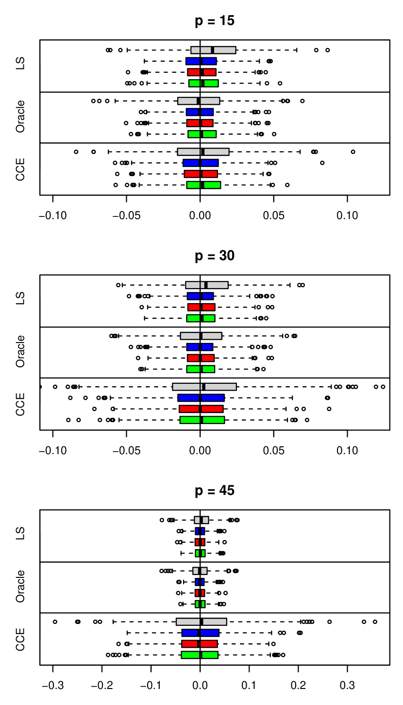
(a) $T=50$

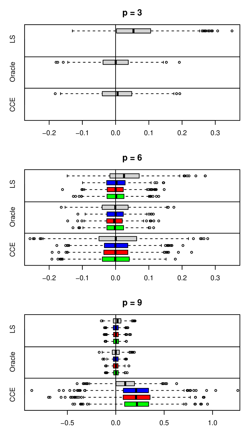
(b) $T=10$

Figure 1: Simulation results in Scenario A.

Figure 1(a) depicts the results for $n=50$, $T=50$ and $p\in\{15,30,45\}$. In each panel, the first four rows with the label “LS” show the box plots for the deviations $\Delta_{\text{LS},j}$ with $j\in\{1,4,4+d,4+2d\}$, the following four rows with the label “Oracle” show the box plots for $\Delta_{\text{LS},j}^{\text{oracle}}$, and the final four rows with the label “CCE” show the box plots for $\Delta_{\text{CCE},j}$. The box plots corresponding to the regressor $j=1$ are in grey and those corresponding to the regressors $j=4$, $j=4+d$ and $j=4+2d$ are in blue, red and green, respectively. In all settings considered in Figure 1(a), the box plots produced by our least squares estimator are nearly indistinguishable from those of the oracle estimator, except for the case with $p=15$ regressors where our estimator is a bit biased for $j=1$. Apart from this minor difference, the estimator performs almost as well as the oracle. Whereas the CCE estimator shows a comparable performance for $p=15$, its performance deteriorates considerably as the number of regressors $p$ gets larger and comes closer to the critical threshold $T$. The behaviour of our estimator, in contrast, is very stable across $p$. This nicely illustrates that unlike the CCE approach, our procedure works well independently of the size of $p$. Figure 1(b) shows the results for $n=50$, the smaller time series length $T=10$ and $p\in\{3,6,9\}$. As can be seen, the results are qualitatively the same as those in Figure 1(a).

6.3 Simulation results in Scenario B

In Scenario B, we compare the lasso and the least squares variant of our estimator, $\widehat{\beta}_{\lambda}$ and $\widehat{\beta}_{\text{LS}}$, with their oracle versions, $\widehat{\beta}_{\lambda}^{\text{oracle}}$ and $\widehat{\beta}_{\text{LS}}^{\text{oracle}}$. The simulation results are again presented via boxplots of the deviations.

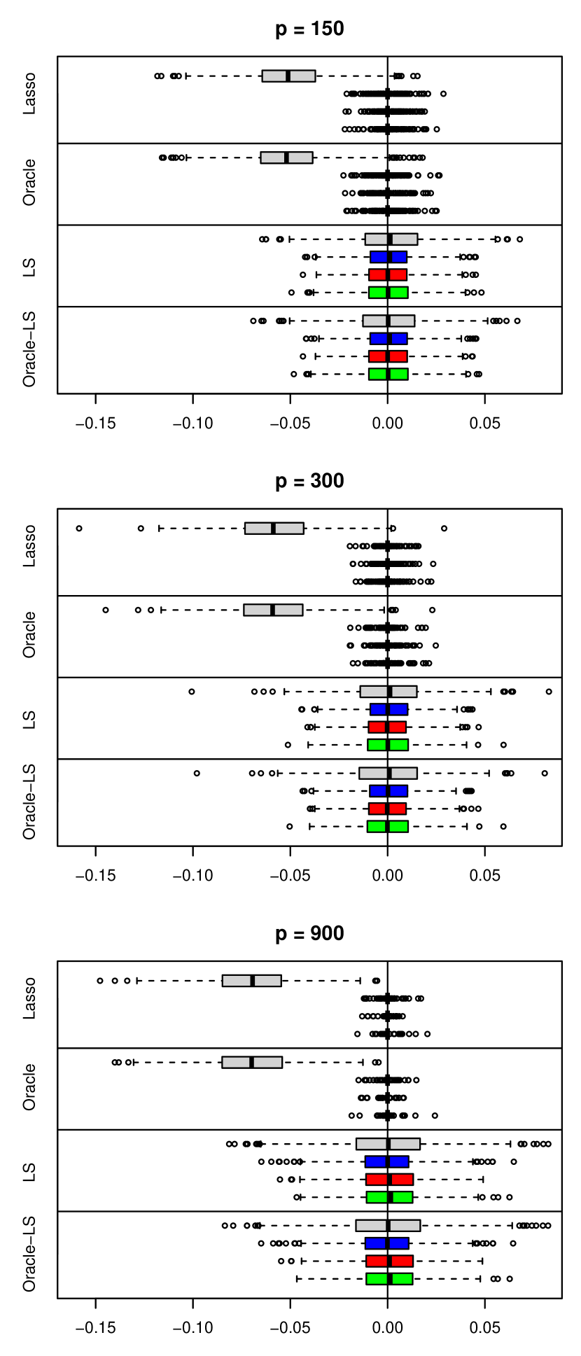
(a) $T=50$

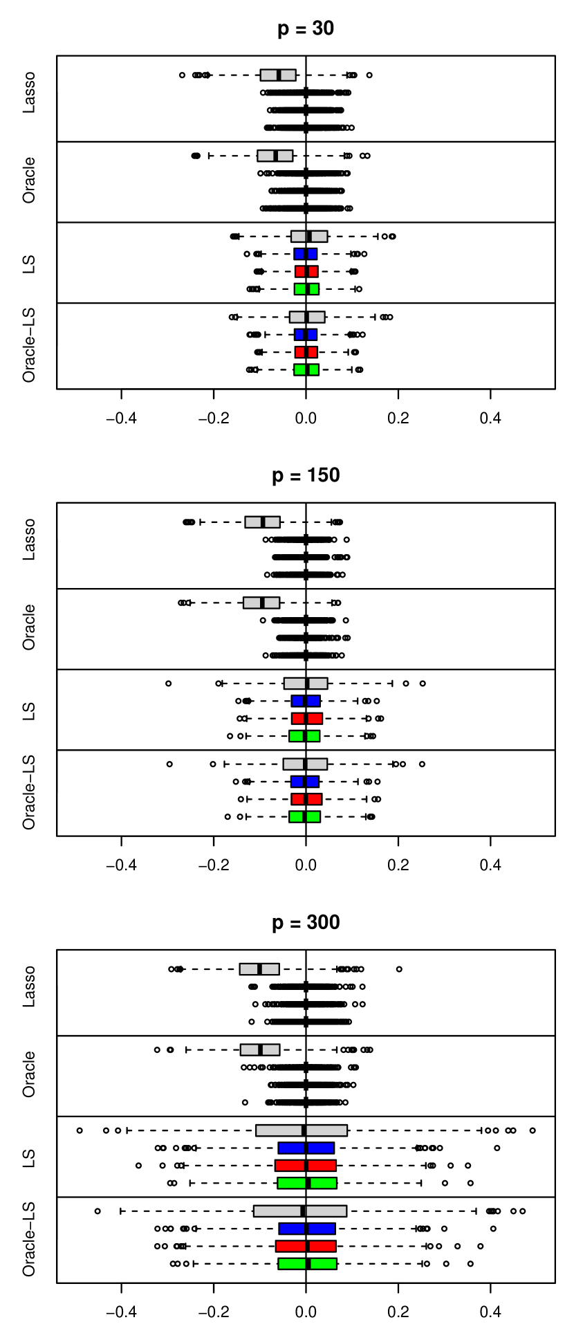
(b) $T=10$

Figure 2: Simulation results in Scenario B.

Figure 2(a) depicts the results for $n=50$, $T=50$ and $p\in\{150,300,900\}$. In each panel, the first four rows with the label “Lasso” show the box plots for the deviations $\Delta_{\lambda,j}=\widehat{\beta}_{\lambda,j}-\beta_{j}$ with $j\in\{1,4,4+d,4+2d\}$, the following four rows with the label “Oracle” show the box plots for $\Delta_{\lambda,j}^{\text{oracle}}=\widehat{\beta}_{\lambda,j}^{\text{oracle}}-\beta_{j}$, the next four rows with the label “LS” show the box plots for $\Delta_{\text{LS},j}$, and the final four rows with the label “Oracle-LS” show the box plots for $\Delta_{\text{LS},j}^{\text{oracle}}$. The box plots produced by our estimators are very similar to those of the corresponding oracle, meaning that the performance of our estimators matches the performance of the respective oracle. Whereas the boxplots of our least squares estimator and its oracle version are approximately centred around $0$, the boxplots of our lasso estimator and its oracle version are biased downwards for $j=1$. This is not surprising because by construction, the lasso shrinks the parameter values towards zero. The box plots of the lasso and its oracle for the components $j=4,4+d,4+2d$ may look a bit strange on first sight: one can only see the set of outliers, whereas the whole region between the whiskers is collapsed to zero. The reason for this is as follows: Since $\beta_{j}=0$ for $j=4,4+d,4+2d$, the lasso $\widehat{\beta}_{\lambda,j}$ often takes exactly the value $0$. Only in a small fraction of the simulation runs, it takes a non-zero value. These non-zero values are visible as outliers in the box plots. Figure 2(b) shows the simulation results for $n=50$, the smaller time series length $T=10$ and $p\in\{30,150,300\}$. The results are qualitatively the same as for $T=50$.

6.4 Simulation results in Scenario C

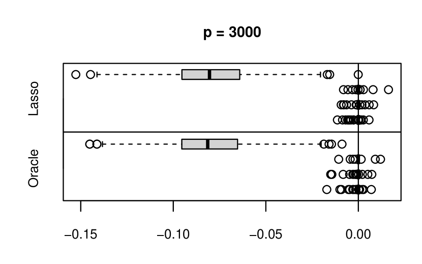
(a) $T=50$

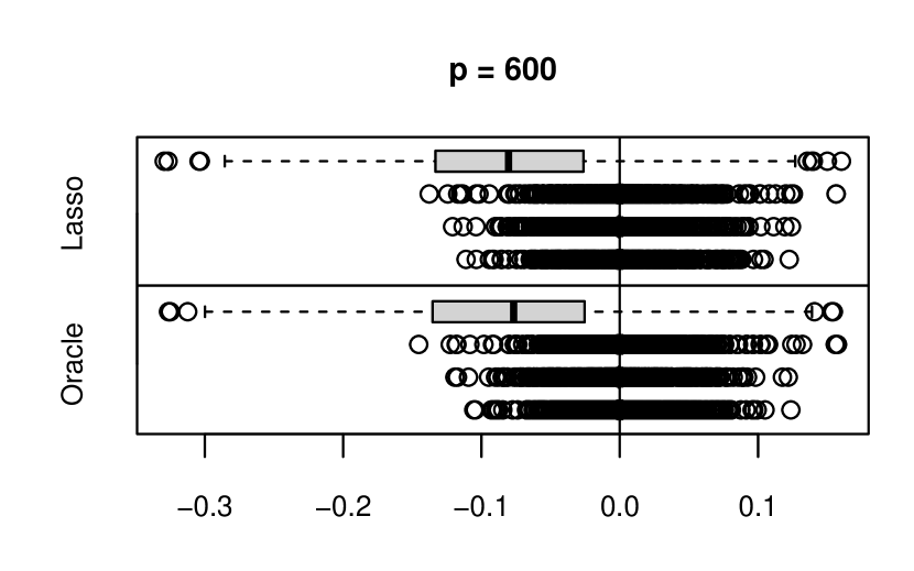
(b) $T=10$

Figure 3: Simulation results in Scenario C.

We finally turn to Scenario C where $p$ exceeds the sample size $nT$. Figure 3(a) shows the simulation results for $n=50$, $T=50$ and $p=3000$. The first four rows with the label “Lasso” display the box plots for the deviations $\Delta_{\lambda,j}$ with $j\in\{1,4,4+d,4+2d\}$ produced by our lasso estimator, and the following four rows with the label “Oracle” display the box plots for $\Delta_{\lambda,j}^{\text{oracle}}$ produced by the corresponding oracle. As in Scenario B, the box plots of the lasso estimator are almost indistinguishable from those of the oracle. Moreover, one can again see a downward bias for $j=1$ and box plots with only outliers for $j\in\{4,4+d,4+2d\}$. Figure 3(b) shows the results for $n=50$, $T=10$ and $p=600$, which are qualitatively the same as those in Figure 3(a).

6.5 Summary

Both the lasso and the least squares variant of our estimator exhibit a performance comparable to the oracle in all the considered settings of Scenarios A–C, even when the number of regressors $p$ is very large. Hence, the simulation exercises demonstrate that our estimation approach works well in higher dimensions and in particular allows to deal with the case $p\geq T$ where the CCE approach is not available.

7 Concluding remarks

In this paper, we have developed new estimation methods for high-dimensional panel data models with interactive fixed effects. Our estimator relies on the following general idea: rather than estimating the unobserved factor structure, we eliminate the factors from the model equation by a projection. Our method can thus be regarded as a high-dimensional analogue of the CCE method which is frequently used in the standard low-dimensional case. The projection device of the CCE approach breaks down completely in high dimensions and a simple fix is not possible. One of the main contributions of the paper is to come up with a novel projection device which works in both low and high dimensions. This device can be combined with high-dimensional regression techniques such as the lasso to obtain an estimator of the unknown parameter vector.

In our theoretical analysis, we have focused on point estimation. Specifically, we have derived the convergence rate of our estimator. Deriving the rate of the estimator is of course only a first step towards a comprehensive theory. The next natural step is to develop distribution theory and to analyze inferential procedures based on the estimator. As this is highly non-trivial and a substantial project in itself, we will tackle this next step in a separate paper. The most influential methods for high-dimensional inference are the desparsified (or de-biased) lasso introduced in Zhang and Zhang (2014) and further developed in van de Geer et al. (2014) and Javanmard and Montanari (2014) and the double selection method of Belloni et al. (2014). Even though theoretically demanding, we conjecture that it is possible to extend these approaches to the setting at hand.

Appendix A: Results on identification

Throughout this and the following appendices, we let $c$ and $C$ denote generic positive constants that may take a different value on each occurrence. The symbols $c_{j}$ and $C_{j}$ with subscript $j$ (which may be either a natural number or a letter) are specific constants that are defined in the course of the appendices. Unless stated differently, the constants $c$, $C$, $c_{j}$ and $C_{j}$ depend neither on the dimensions $n$, $T$, $p$ nor on the sparsity index $s$. To emphasize that they do not depend on any of these parameters, we sometimes refer to them as absolute constants.

Proof of Lemma 3.1..

By Lemma B.3, the eigenvalues $\overline{\psi}_{1}\geq\ldots\geq\overline{\psi}_{p}\geq 0$ of the $p\times p$ matrix $\overline{\boldsymbol{\Sigma}}=\mathbb{E}[T^{-1}\sum_{t=1}^{T}\overline{X}_{t}\overline{X}_{t}^{\top}]$ have the following property for sufficiently large $n$: there exists a constant $c_{0}>0$ such that

$$\overline{\psi}_{k}\geq c_{0}\,p\quad\text{for all }k\leq K,$$

whereas $\overline{\psi}_{k}=O(p/\sqrt{T}+p/n)$ for all $k>K$. From this, it immediately follows that

$$K=\sum_{j=1}^{p}1\Big{(}\overline{\psi}_{j}>\frac{c_{0}\,p}{2}\Big{)}$$

for sufficiently large $n$. Hence, $K$ can be expressed as a function of the eigenvalues of the matrix $\mathbb{E}[T^{-1}\sum_{t=1}^{T}\overline{X}_{t}\overline{X}_{t}^{\top}]$, which is uniquely determined by the data. As a result, $K$ is identified. ∎

Proof of Lemma 3.2..

The proof is by contradiction. Suppose there are two $s$-sparse vectors $\beta$ and $\beta^{\prime}$ with active sets $S$ and $S^{\prime}$, respectively, that satisfy model (2.3). Let $\mathbb{E}_{\boldsymbol{f}}[\,\cdot\,]=\mathbb{E}[\,\cdot\,|\boldsymbol{F}=\boldsymbol{f}]$ be the expectation conditional on $\boldsymbol{F}=\boldsymbol{f}$, where $\boldsymbol{f}$ is a fixed realization of the factor matrix $\boldsymbol{F}$. Since

$$\mathbb{E}_{\boldsymbol{f}}\big{\|}Y^{\perp}-\boldsymbol{X}^{\perp}b\big{\|}^{2} =(\beta-b)^{\top}\mathbb{E}_{\boldsymbol{f}}\big{[}(\boldsymbol{X}^{\perp})^{\top}\boldsymbol{X}^{\perp}\big{]}(\beta-b)+\mathbb{E}_{\boldsymbol{f}}\big{[}(\varepsilon^{\perp})^{\top}\varepsilon^{\perp}\big{]}$$

for any $b\in\mathbb{R}^{p}$, $\beta$ minimizes the function $Q(b):=\mathbb{E}_{\boldsymbol{f}}\|Y^{\perp}-\boldsymbol{X}^{\perp}b\|^{2}$. By the same argument, $\beta^{\prime}$ must be a minimizer of $Q(b)$ as well, which implies that

$$(\beta-\beta^{\prime})^{\top}\mathbb{E}_{\boldsymbol{f}}\big{[}(\boldsymbol{X}^{\perp})^{\top}\boldsymbol{X}^{\perp}\big{]}(\beta-\beta^{\prime})=0$$

for any realization $\boldsymbol{f}$ and thus

$$(\beta-\beta^{\prime})^{\top}\mathbb{E}\big{[}(\boldsymbol{X}^{\perp})^{\top}\boldsymbol{X}^{\perp}\big{]}(\beta-\beta^{\prime})=0.$$ (A.1)

Since $\beta-\beta^{\prime}$ is a $2s$-sparse vector whose active set is contained in $I:=S\cup S^{\prime}$, we get by (ID_ℓ3) that

$$\|\boldsymbol{X}^{\perp}(\beta-\beta^{\prime})\|^{2}\geq\frac{nT\varphi^{2}}{2s}\|\beta_{I}-\beta_{I}^{\prime}\|_{1}^{2}>0$$

with probability $\geq 1-c_{n,T}$. Hence, for sufficiently large sample sizes,

$$\mathbb{E}\|\boldsymbol{X}^{\perp}(\beta-\beta^{\prime})\|^{2}=(\beta-\beta^{\prime})^{\top}\mathbb{E}\big{[}(\boldsymbol{X}^{\perp})^{\top}\boldsymbol{X}^{\perp}\big{]}(\beta-\beta^{\prime})>0,$$

which contradicts (A.1). ∎

Proof of Lemma 3.3..

In order to show that $K$ is identified, we can proceed in the same way as in the proof of Lemma 3.1. We only need to invoke Lemma C.3 rather than Lemma B.3. Furthermore, the arguments in the proof of Lemma 3.2 entail that under (ID_s3), the $s$-sparse parameter vector $\beta$ is unique for sufficiently large $n$ conditionally on the realization $\boldsymbol{F}=\boldsymbol{f}$. We thus also get identification of $\beta$. ∎

Appendix B: Proof of Theorem 5.1

In this appendix, we give an overview of the main arguments required to prove Theorem 5.1. The proofs of some intermediate lemmas which are lengthy and tedious to derive are deferred to the Supplementary Material. We thereby attempt to draw a clear picture of the overall proof strategy. We assume throughout that the conditions of Theorem 5.1 are satisfied. Under these conditions, the matrices $\boldsymbol{F}^{\top}\boldsymbol{F}$, $\boldsymbol{W}^{\top}\boldsymbol{W}$ and $\widehat{\boldsymbol{W}}^{\top}\widehat{\boldsymbol{W}}$ are invertible with probability tending to $1$. Hence, we can replace the generalized inverses in the definition of the projection matrices $\boldsymbol{\Pi}$ and $\widehat{\boldsymbol{\Pi}}$ by proper inverses. More precisely speaking, we can write $\boldsymbol{\Pi}=\boldsymbol{I}-\boldsymbol{F}(\boldsymbol{F}^{\top}\boldsymbol{F})^{-1}\boldsymbol{F}^{\top}=\boldsymbol{I}-\boldsymbol{W}(\boldsymbol{W}^{\top}\boldsymbol{W})^{-1}\boldsymbol{W}^{\top}$ and $\widehat{\boldsymbol{\Pi}}=\boldsymbol{I}-\widehat{\boldsymbol{W}}(\widehat{\boldsymbol{W}}^{\top}\widehat{\boldsymbol{W}})^{-1}\widehat{\boldsymbol{W}}^{\top}$ with probability tending to $1$. In what follows, we make use of these formulations but often suppress the specifier “with probability tending to $1$” for simplicity.

Step 1: Analysis of the eigenstructure of $\boldsymbol{\widehat{\Sigma}}$

The matrix $\widehat{\boldsymbol{\Sigma}}=T^{-1}\sum_{t=1}^{T}\overline{X}_{t}\overline{X}_{t}^{\top}$ is an estimator of $\overline{\boldsymbol{\Sigma}}=\mathbb{E}[T^{-1}\sum_{t=1}^{T}\overline{X}_{t}\overline{X}_{t}^{\top}]$. Since $\overline{X}_{t}=\boldsymbol{\Gamma}F_{t}+u_{t}$ with $u_{t}=(\overline{\boldsymbol{\Gamma}}-\boldsymbol{\Gamma})F_{t}+\overline{Z}_{t}$, the matrix $\overline{\boldsymbol{\Sigma}}$ has the form

$$\overline{\boldsymbol{\Sigma}}=\boldsymbol{\Sigma}+\boldsymbol{\Sigma}_{\Delta}+\boldsymbol{\Sigma}_{u},$$

where $\boldsymbol{\Sigma}=\boldsymbol{\Gamma}\boldsymbol{\Gamma}^{\top}$, $\boldsymbol{\Sigma}_{\Delta}=\boldsymbol{\Gamma}\{\mathbb{E}[T^{-1}\sum_{t=1}^{T}F_{t}F_{t}^{\top}]-\boldsymbol{I}_{K}\}\boldsymbol{\Gamma}^{\top}$ and $\boldsymbol{\Sigma}_{u}=\mathbb{E}[T^{-1}\sum_{t=1}^{T}u_{t}u_{t}^{\top}]$. We first derive some rough bounds on the distances between the matrices $\boldsymbol{\Sigma}$, $\overline{\boldsymbol{\Sigma}}$ and $\widehat{\boldsymbol{\Sigma}}$.

Lemma B.1.

It holds that

1. $\displaystyle{\|\widehat{\boldsymbol{\Sigma}}-\overline{\boldsymbol{\Sigma}}\|=O_{p}\Big{(}\frac{p}{\sqrt{T}}+\frac{p\sqrt{\log p}}{\sqrt{n}}\Big{)}}$.

2. $\displaystyle{\|\overline{\boldsymbol{\Sigma}}-\boldsymbol{\Sigma}\|=O\Big{(}\frac{p}{\sqrt{T}}+\frac{p}{n}\Big{)}}$.

With these bounds at hand, we have a closer look at the eigenstructure of the matrices $\boldsymbol{\Sigma}$, $\overline{\boldsymbol{\Sigma}}$ and $\widehat{\boldsymbol{\Sigma}}$. The first result shows that the matrix $\boldsymbol{\Sigma}$ has spiked eigenvalues: its first $K$ eigenvalues are extremely large (in particular, of order $p$) whereas the others are equal to $0$.

Lemma B.2.

The eigenvalues $\psi_{1}\geq\ldots\geq\psi_{p}\geq 0$ of the matrix $\boldsymbol{\Sigma}$ have the following property: there exists an absolute constant $c_{0}>0$ such that

$$\psi_{k}\geq c_{0}\,p\quad\text{for all }k\leq K,$$

whereas $\psi_{k}=0$ for all $k>K$.

Proof of Lemma B.2..

The claim follows upon considering the singular value decomposition $\boldsymbol{\Gamma}=\boldsymbol{U}\boldsymbol{D}\boldsymbol{V}^{\top}$, where the matrices $\boldsymbol{U}\in\mathbb{R}^{p\times K}$ and $\boldsymbol{V}\in\mathbb{R}^{K\times K}$ have orthonormal columns and $\boldsymbol{D}=\text{diag}(d_{1},\ldots,d_{K})$ is a diagonal matrix with $d_{1}\geq\ldots\geq d_{K}\geq 0$. With this decomposition, we get that

$$\boldsymbol{\Sigma}/p=\boldsymbol{\Gamma}\boldsymbol{\Gamma}^{\top}/p=\boldsymbol{U}(\boldsymbol{D}^{2}/p)\boldsymbol{U}^{\top},$$

which implies that the first $K$ eigenvalues of $\boldsymbol{\Sigma}/p=\boldsymbol{\Gamma}\boldsymbol{\Gamma}^{\top}/p$ are $d_{1}^{2}/p\geq\ldots\geq d_{K}^{2}/p$, while the others are equal to $0$. Since the first $K$ eigenvalues of $\boldsymbol{\Sigma}/p=\boldsymbol{\Gamma}\boldsymbol{\Gamma}^{\top}/p$ are identical to those of $\boldsymbol{\Gamma}^{\top}\boldsymbol{\Gamma}/p$, (ID_ℓ2) yields that $0<c_{\min}\leq d_{K}^{2}/p\leq\ldots\leq d_{1}^{2}/p\leq c_{\max}<\infty$. From this, the statement of the lemma follows immediately. ∎

The next lemma shows that the matrix $\overline{\boldsymbol{\Sigma}}$ has spiked eigenvalues as well. More specifically, the first $K$ eigenvalues are of the order $p$ whereas the others are of substantially smaller order.

Lemma B.3.

The eigenvalues $\overline{\psi}_{1}\geq\ldots\geq\overline{\psi}_{p}\geq 0$ of $\overline{\boldsymbol{\Sigma}}$ have the following property: there exist an absolute constant $c_{0}>0$ and a natural number $n_{0}$ such that

$$\overline{\psi}_{k}\geq c_{0}\,p\quad\text{for all }k\leq K\text{ and }n\geq n_{0},$$

whereas $\overline{\psi}_{k}=O(p/\sqrt{T}+p/n)$ for all $k>K$.

Proof of Lemma B.3..

By Lemma B.1, $\|\overline{\boldsymbol{\Sigma}}-\boldsymbol{\Sigma}\|=O(p/\sqrt{T}+p/n)$. Hence, Weyl’s theorem yields that

$$|\overline{\psi}_{k}-\psi_{k}|\leq\|\overline{\boldsymbol{\Sigma}}-\boldsymbol{\Sigma}\|=O\Big{(}\frac{p}{\sqrt{T}}+\frac{p}{n}\Big{)}$$ (B.1)

for any $k$. Since $\psi_{k}\geq c_{0}p$ for $k\leq K$ and $\psi_{k}=0$ for $k>K$ by Lemma B.2, the lemma follow immediately from (B.1). ∎

We finally verify that the sample autocovariance matrix $\widehat{\boldsymbol{\Sigma}}$ has spiked eigenvalues similar to $\boldsymbol{\Sigma}$ and $\overline{\boldsymbol{\Sigma}}$.

Lemma B.4.

The eigenvalues $\widehat{\psi}_{1}\geq\ldots\geq\widehat{\psi}_{p}\geq 0$ of $\widehat{\boldsymbol{\Sigma}}$ have the following property: there exists an absolute constant $c_{0}>0$ such that with probability tending to $1$,

$$\widehat{\psi}_{k}\geq c_{0}\,p\quad\text{for }k\leq K,$$

whereas $\widehat{\psi}_{k}=O_{p}(p/\sqrt{T}+p\sqrt{\log p}/\sqrt{n})=o_{p}(p)$ for all $k>K$.

Proof of Lemma B.4..

Using that $\|\widehat{\boldsymbol{\Sigma}}-\overline{\boldsymbol{\Sigma}}\|=O_{p}(p/\sqrt{T}+p\sqrt{\log p}/\sqrt{n})$, we can argue analogously as in the proof of Lemma B.3. ∎

An immediate consequence of the above lemmas is the following.

Lemma B.5.

It holds that $\widehat{K}\stackrel{{\scriptstyle p}}{{\longrightarrow}}K$.

Put differently, $\widehat{K}=K$ with probability tending to $1$.

Step 2: Analysis of the projection matrix $\boldsymbol{\widehat{\Pi}}$

In this step, we aim to link the proxy $\boldsymbol{\widehat{\Pi}}$ of our method to the unknown projection matrix $\boldsymbol{\Pi}$. With $\widehat{\boldsymbol{W}}=\overline{\boldsymbol{X}}\widehat{\boldsymbol{U}}=\boldsymbol{F}\overline{\boldsymbol{\Gamma}}^{\top}\widehat{\boldsymbol{U}}+\overline{\boldsymbol{Z}}\widehat{\boldsymbol{U}}$, we can write $\widehat{\boldsymbol{\Pi}}$ as

$$\widehat{\boldsymbol{\Pi}} =\boldsymbol{I}-\widehat{\boldsymbol{W}}(\widehat{\boldsymbol{W}}^{\top}\widehat{\boldsymbol{W}})^{-1}\widehat{\boldsymbol{W}}^{\top}$$

$$=\bigg{\{}\boldsymbol{I}-\frac{1}{T}(\boldsymbol{F}\overline{\boldsymbol{\Gamma}}^{\top}\widehat{\boldsymbol{U}})\Big{[}\frac{1}{T}(\boldsymbol{F}\overline{\boldsymbol{\Gamma}}^{\top}\widehat{\boldsymbol{U}})^{\top}(\boldsymbol{F}\overline{\boldsymbol{\Gamma}}^{\top}\widehat{\boldsymbol{U}})\Big{]}^{-1}(\boldsymbol{F}\overline{\boldsymbol{\Gamma}}^{\top}\widehat{\boldsymbol{U}})^{\top}\bigg{\}}-\widehat{\boldsymbol{R}},$$

where

$$\widehat{\boldsymbol{R}} =\frac{1}{T}(\boldsymbol{F}\overline{\boldsymbol{\Gamma}}^{\top}\widehat{\boldsymbol{U}})\bigg{\{}\widehat{\boldsymbol{\Psi}}^{-1}-\Big{[}\frac{1}{T}(\boldsymbol{F}\overline{\boldsymbol{\Gamma}}^{\top}\widehat{\boldsymbol{U}})^{\top}(\boldsymbol{F}\overline{\boldsymbol{\Gamma}}^{\top}\widehat{\boldsymbol{U}})\Big{]}^{-1}\bigg{\}}(\boldsymbol{F}\overline{\boldsymbol{\Gamma}}^{\top}\widehat{\boldsymbol{U}})^{\top}$$

$$\quad+\frac{1}{T}(\boldsymbol{F}\overline{\boldsymbol{\Gamma}}^{\top}\widehat{\boldsymbol{U}})\widehat{\boldsymbol{\Psi}}^{-1}(\overline{\boldsymbol{Z}}\widehat{\boldsymbol{U}})^{\top}$$

$$\quad+\frac{1}{T}(\overline{\boldsymbol{Z}}\widehat{\boldsymbol{U}})\widehat{\boldsymbol{\Psi}}^{-1}(\boldsymbol{F}\overline{\boldsymbol{\Gamma}}^{\top}\widehat{\boldsymbol{U}})^{\top}$$

$$\quad+\frac{1}{T}(\overline{\boldsymbol{Z}}\widehat{\boldsymbol{U}})\widehat{\boldsymbol{\Psi}}^{-1}(\overline{\boldsymbol{Z}}\widehat{\boldsymbol{U}})^{\top}$$

and

$$\frac{\widehat{\boldsymbol{W}}^{\top}\widehat{\boldsymbol{W}}}{T}=\widehat{\boldsymbol{U}}^{\top}\Big{(}\frac{\overline{\boldsymbol{X}}^{\top}\overline{\boldsymbol{X}}}{T}\Big{)}\widehat{\boldsymbol{U}}=\widehat{\boldsymbol{U}}^{\top}\widehat{\boldsymbol{\Sigma}}\widehat{\boldsymbol{U}}=\text{diag}(\widehat{\psi}_{1},\ldots,\widehat{\psi}_{\widehat{K}})=:\widehat{\boldsymbol{\Psi}}.$$

We now relate the two projection matrices $\boldsymbol{\widehat{\Pi}}$ and $\boldsymbol{\Pi}$ to each other. The main observation to achieve this is stated in the following lemma.

Lemma B.6.

The random matrix $\overline{\boldsymbol{\Gamma}}^{\top}\widehat{\boldsymbol{U}}$ is invertible with probability tending to $1$.

This lemma implies that with probability tending to $1$, the column vectors of $\boldsymbol{F}\overline{\boldsymbol{\Gamma}}^{\top}\widehat{\boldsymbol{U}}$ span the same linear subspace of $\mathbb{R}^{T}$ as the factors $\boldsymbol{F}$. Consequently, we can represent the projection matrix $\boldsymbol{\Pi}=\boldsymbol{I}-\boldsymbol{F}(\boldsymbol{F}^{\top}\boldsymbol{F})^{-1}\boldsymbol{F}^{\top}$ as

$$\boldsymbol{\Pi}=\boldsymbol{I}-\frac{1}{T}(\boldsymbol{F}\overline{\boldsymbol{\Gamma}}^{\top}\widehat{\boldsymbol{U}})\Big{[}\frac{1}{T}(\boldsymbol{F}\overline{\boldsymbol{\Gamma}}^{\top}\widehat{\boldsymbol{U}})^{\top}(\boldsymbol{F}\overline{\boldsymbol{\Gamma}}^{\top}\widehat{\boldsymbol{U}})\Big{]}^{-1}(\boldsymbol{F}\overline{\boldsymbol{\Gamma}}^{\top}\widehat{\boldsymbol{U}})^{\top}$$

with probability tending to $1$. As a result, we obtain the following.

Lemma B.7.

With probability tending to $1$, $\widehat{\boldsymbol{\Pi}}=\boldsymbol{\Pi}-\widehat{\boldsymbol{R}}$.

Lemma B.7 allows us to decompose the observed projection matrix $\widehat{\boldsymbol{\Pi}}$ into the “oracle” projection matrix $\boldsymbol{\Pi}$, which presupposes knowledge of the factors $\boldsymbol{F}$, and a remainder term $\widehat{\boldsymbol{R}}$. In order to exploit this decomposition, we need to make sure that the approximation error produced by the remainder $\widehat{\boldsymbol{R}}$ is asymptotically negligible. To do so, we examine the behaviour of the various components that show up in $\widehat{\boldsymbol{R}}$. This is done in the Supplementary Material, in particular in Lemma S.6 and the proofs of Lemmas B.9 and B.10.

Step 3: Analysis of the lasso $\boldsymbol{\widehat{\beta}_{\lambda}}$

The lasso $\widehat{\beta}_{\lambda}$ can be formulated as

$$\widehat{\beta}_{\lambda}\in\underset{b\in\mathbb{R}^{p}}{\text{argmin}}\bigg{\{}\frac{1}{nT}\big{\|}\widehat{Y}-\widehat{\boldsymbol{X}}b\big{\|}^{2}+\lambda\|b\|_{1}\bigg{\}}$$

with $\widehat{Y}=(\widehat{Y}_{1},\ldots,\widehat{Y}_{n})^{\top}$ and $\widehat{\boldsymbol{X}}=(\widehat{\boldsymbol{X}}_{1}^{\top}\ldots\widehat{\boldsymbol{X}}_{n}^{\top})^{\top}$. Let $\mathcal{T}_{\text{RE}}$ be the event that the design matrix $\widehat{\boldsymbol{X}}$ fulfills the $\text{RE}(S,\phi)$ condition with some constant $\phi>0$ and define the event $\mathcal{T}_{\lambda}$ as

$$\mathcal{T}_{\lambda}=\Big{\{}\frac{4\|\widehat{\boldsymbol{X}}^{\top}e\|_{\infty}}{nT}\leq\lambda\Big{\}},$$

where $e=(e_{1}^{\top},\ldots,e_{n}^{\top})^{\top}$ with $e_{i}=\boldsymbol{F}\gamma_{i}+\varepsilon_{i}$. We first show that the lasso is well-behaved on the event $\mathcal{T}_{\lambda}\cap\mathcal{T}_{\text{RE}}$ in the following sense.

Lemma B.8.

On the event $\mathcal{T}_{\lambda}\cap\mathcal{T}_{\textnormal{RE}}$, it holds that

$$\|\widehat{\beta}_{\lambda}-\beta\|_{1}\leq\frac{4}{\phi^{2}}\lambda s.$$

Lemma B.8 follows from standard finite-sample theory for the lasso. A proof is provided in the Supplementary Material for completeness.

We next have a closer look at the events $\mathcal{T}_{\lambda}$ and $\mathcal{T}_{\text{RE}}$ that show up in Lemma B.8. If we can prove that these two events occur with probability tending to $1$ for sufficiently small values of $\lambda$, Theorem 5.1 is an immediate consequence of Lemma B.8. In order to deal with the event $\mathcal{T}_{\lambda}$, we derive the convergence rate of $\|\widehat{\boldsymbol{X}}^{\top}e\|_{\infty}/(nT)$, which is stated in the following lemma.

Lemma B.9.

It holds that

$$\frac{\|\widehat{\boldsymbol{X}}^{\top}e\|_{\infty}}{nT}=O_{p}\Big{(}\frac{\log pT}{n}+\sqrt{\frac{\log(npT)\log(np)}{nT}}\Big{)}.$$

Roughly speaking, the strategy to prove Lemma B.9 is as follows: Let $X_{i,j}$ be the $j$-th column of $\boldsymbol{X}_{i}$, $Z_{i,j}$ the $j$-th column of $\boldsymbol{Z}_{i}$ and $\Gamma_{i,j}$ the $j$-th row of $\boldsymbol{\Gamma}_{i}$. We write

$$\frac{\|\widehat{\boldsymbol{X}}^{\top}e\|_{\infty}}{nT}=\frac{1}{nT}\max_{1\leq j\leq p}\Big{|}\sum_{i=1}^{n}\widehat{X}_{i,j}^{\top}e_{i}\Big{|}$$

along with

$$\sum_{i=1}^{n}\widehat{X}_{i,j}^{\top}e_{i}=\sum_{i=1}^{n}\big{\{}\widehat{\boldsymbol{\Pi}}X_{i,j}\big{\}}^{\top}\big{\{}\widehat{\boldsymbol{\Pi}}e_{i}\big{\}}=\sum_{i=1}^{n}\big{\{}\widehat{\boldsymbol{\Pi}}(\boldsymbol{F}\Gamma_{i,j}+Z_{i,j})\big{\}}^{\top}\big{\{}\widehat{\boldsymbol{\Pi}}(\boldsymbol{F}\gamma_{i}+\varepsilon_{i})\big{\}}$$

and exploit the main result from Step 2 in these formulas, according to which $\widehat{\boldsymbol{\Pi}}=\boldsymbol{\Pi}-\widehat{\boldsymbol{R}}$ with probability tending to $1$. The details are provided in the Supplementary Material. From Lemma B.9, it immediately follows that

$$\mathbb{P}(\mathcal{T}_{\lambda})\to 1\quad\text{for any choice}\quad\lambda=h_{n}\frac{\log(npT)}{\min\{n,\sqrt{nT}\}},$$ (B.2)

where $h_{n}$ slowly diverges to infinity. Hence, $\mathcal{T}_{\lambda}$ occurs with probability tending to $1$ if $\lambda$ is chosen of slightly larger order than $1/\min\{n,\sqrt{nT}\}$.

In order to cope with the event $\mathcal{T}_{\text{RE}}$, we first show that the covariance matrix $\widehat{\boldsymbol{X}}^{\top}\widehat{\boldsymbol{X}}/(nT)$ is close to $\boldsymbol{Z}^{\top}\boldsymbol{Z}/(nT)$ in the following sense.

Lemma B.10.

It holds that

$$\Big{\|}\frac{\widehat{\boldsymbol{X}}^{\top}\widehat{\boldsymbol{X}}}{nT}-\frac{\boldsymbol{Z}^{\top}\boldsymbol{Z}}{nT}\Big{\|}_{\max}=O_{p}\Big{(}\frac{\log(npT)}{\min\{n,T\}}\Big{)}.$$

The proof strategy is similar to that for Lemma B.9. In particular, we rewrite the term of interest in a suitable way and then make heavy use of the fact that $\widehat{\boldsymbol{\Pi}}=\boldsymbol{\Pi}-\widehat{\boldsymbol{R}}$ with probability tending to $1$. The details are again deferred to the Supplementary Material. Since $s=o(\min\{n,T\}/\log(npT))$ by (D_ℓ2), Lemma B.10 implies that

$$\frac{32s}{\varphi^{2}}\Big{\|}\frac{\widehat{\boldsymbol{X}}^{\top}\widehat{\boldsymbol{X}}}{nT}-\frac{\boldsymbol{Z}^{\top}\boldsymbol{Z}}{nT}\Big{\|}_{\max}\leq 1$$ (B.3)

with probability tending to $1$ for any given constant $\varphi>0$. We can now use Corollary 6.8 in Bühlmann and van de Geer (2011), which says the following when applied to our context: Whenever $\boldsymbol{Z}$ fulfills the $\text{RE}(S,\varphi)$ condition and (B.3) is fulfilled, $\widehat{\boldsymbol{X}}$ satisfies the $\text{RE}(S,\phi)$ condition with $\phi=\varphi/\sqrt{2}$. Since $\boldsymbol{Z}$ obeys the $\text{RE}(S,\varphi)$ condition with probability tending to $1$ by assumption, we can infer that $\widehat{\boldsymbol{X}}$ must satisfy the $\text{RE}(S,\phi)$ condition with probability tending to $1$, that is,

$$\mathbb{P}(\mathcal{T}_{\text{RE}})\to 1.$$ (B.4)

Combining Lemma B.8 with (B.2) and (B.4), we finally arrive at the following statement:

$$\|\widehat{\beta}_{\lambda}-\beta\|_{1}\leq\frac{4}{\phi^{2}}\lambda s$$

for any $\lambda=h_{n}\log(npT)/\min\{n,\sqrt{nT}\}$ with probability tending to $1$, which implies Theorem 5.1.

Appendix C: Proof of Theorem 5.2

The proof strategy is the same as in the large-$T$-case. The various lemmas and auxiliary results, however, that are derived in the three main steps of the proof must be adapted. As they can be adapted in a quite straightforward way, we do not give full proofs but only comment on noteworthy differences. We make use of the shorthands $\mathbb{P}_{\boldsymbol{f}}(\,\cdot\,)=\mathbb{P}(\,\cdot\,|\boldsymbol{F}=\boldsymbol{f})$ and $\mathbb{E}_{\boldsymbol{f}}[\,\cdot\,]=\mathbb{E}[\,\cdot\,|\boldsymbol{F}=\boldsymbol{f}]$ and assume throughout that the conditions of Theorem 5.2 are fulfilled.

Step 1: Analysis of the eigenstructure of $\boldsymbol{\widehat{\Sigma}}$

Similar to the large-$T$-case, we use the notation $\widehat{\boldsymbol{\Sigma}}=T^{-1}\sum_{t=1}^{T}\overline{X}_{t}\overline{X}_{t}^{\top}$ and $\overline{\boldsymbol{\Sigma}}=\mathbb{E}_{\boldsymbol{f}}[T^{-1}\sum_{t=1}^{T}\overline{X}_{t}\overline{X}_{t}^{\top}]$. Since $\overline{X}_{t}=\boldsymbol{\Gamma}F_{t}+u_{t}$ with $u_{t}=(\overline{\boldsymbol{\Gamma}}-\boldsymbol{\Gamma})F_{t}+\overline{Z}_{t}$ and the factors are normalized such that $T^{-1}\sum_{t=1}^{T}f_{t}f_{t}^{\top}=\boldsymbol{f}^{\top}\boldsymbol{f}/T=\boldsymbol{I}_{K}$, we can further write $\overline{\boldsymbol{\Sigma}}=\boldsymbol{\Sigma}+\boldsymbol{\Sigma}_{u}$ with $\boldsymbol{\Sigma}:=\boldsymbol{\Gamma}\boldsymbol{\Gamma}^{\top}$ and $\boldsymbol{\Sigma}_{u}:=\mathbb{E}_{\boldsymbol{f}}[T^{-1}\sum_{t=1}^{T}u_{t}u_{t}^{\top}]$. In what follows, we state versions of Lemmas B.1–B.5 for the small-$T$-case. The proofs are analogous to those of Lemmas B.1–B.5 and are thus omitted.

Lemma C.1.

Conditionally on $\boldsymbol{F}=\boldsymbol{f}$, it holds that

1. $\displaystyle{\|\widehat{\boldsymbol{\Sigma}}-\overline{\boldsymbol{\Sigma}}\|=O_{p}\Big{(}p\sqrt{\frac{\log p}{n}}\Big{)}}$.

2. $\displaystyle{\|\overline{\boldsymbol{\Sigma}}-\boldsymbol{\Sigma}\|=O\Big{(}\frac{p}{n}\Big{)}}$.

Lemma C.2.

Conditionally on $\boldsymbol{F}=\boldsymbol{f}$, the eigenvalues $\psi_{1}\geq\ldots\geq\psi_{p}\geq 0$ of $\boldsymbol{\Sigma}$ have the following property: there exists an absolute constant $c_{0}>0$ such that

$$\psi_{k}\geq c_{0}\,p\quad\text{for all }k\leq K,$$

whereas $\psi_{k}=0$ for all $k>K$.

Lemma C.3.

Conditionally on $\boldsymbol{F}=\boldsymbol{f}$, the eigenvalues $\overline{\psi}_{1}\geq\ldots\geq\overline{\psi}_{p}\geq 0$ of $\overline{\boldsymbol{\Sigma}}$ have the following property: there exist an absolute constant $c_{0}>0$ and a natural number $n_{0}$ such that

$$\overline{\psi}_{k}\geq c_{0}\,p\quad\text{for all }k\leq K\text{ and }n\geq n_{0},$$

whereas $\overline{\psi}_{k}=O(p/n)$ for all $k>K$.

Lemma C.4.

Conditionally on $\boldsymbol{F}=\boldsymbol{f}$, the eigenvalues $\widehat{\psi}_{1}\geq\ldots\geq\widehat{\psi}_{p}\geq 0$ of $\widehat{\boldsymbol{\Sigma}}$ have the following property: there exists an absolute constant $c_{0}>0$ such that with probability tending to $1$,

$$\widehat{\psi}_{k}\geq c_{0}\,p\quad\text{for }k\leq K,$$

whereas $\widehat{\psi}_{k}=O_{p}(p\sqrt{\log p}/\sqrt{n})=o_{p}(p)$ for all $k>K$.

Lemma C.5.

Conditionally on $\boldsymbol{F}=\boldsymbol{f}$, it holds that $\widehat{K}\stackrel{{\scriptstyle p}}{{\longrightarrow}}K$.

Step 2: Analysis of the projection matrix $\boldsymbol{\widehat{\Pi}}$

We decompose $\boldsymbol{\widehat{\Pi}}$ exactly as in Appendix B. In particular, we write

$$\widehat{\boldsymbol{\Pi}} =\boldsymbol{I}-\widehat{\boldsymbol{W}}(\widehat{\boldsymbol{W}}^{\top}\widehat{\boldsymbol{W}})^{-1}\widehat{\boldsymbol{W}}^{\top}$$

$$=\bigg{\{}\boldsymbol{I}-\frac{1}{T}(\boldsymbol{F}\overline{\boldsymbol{\Gamma}}^{\top}\widehat{\boldsymbol{U}})\Big{[}\frac{1}{T}(\boldsymbol{F}\overline{\boldsymbol{\Gamma}}^{\top}\widehat{\boldsymbol{U}})^{\top}(\boldsymbol{F}\overline{\boldsymbol{\Gamma}}^{\top}\widehat{\boldsymbol{U}})\Big{]}^{-1}(\boldsymbol{F}\overline{\boldsymbol{\Gamma}}^{\top}\widehat{\boldsymbol{U}})^{\top}\bigg{\}}-\widehat{\boldsymbol{R}},$$

where $\widehat{\boldsymbol{W}}=\overline{\boldsymbol{X}}\widehat{\boldsymbol{U}}$ and $\widehat{\boldsymbol{R}}$ is defined as before. This decomposition allows us to link the proxy $\widehat{\boldsymbol{\Pi}}$ to the unknown projection matrix $\boldsymbol{\Pi}$ in the same way as in the large-$T$-case. Specifically, by arguments completely analogous to those for Lemmas B.6 and B.7, we can prove the following.

Lemma C.6.

Conditionally on $\boldsymbol{F}=\boldsymbol{f}$, the random matrix $\overline{\boldsymbol{\Gamma}}^{\top}\widehat{\boldsymbol{U}}$ is invertible with probability tending to $1$.

Lemma C.7.

Conditionally on $\boldsymbol{F}=\boldsymbol{f}$, it holds that $\widehat{\boldsymbol{\Pi}}=\boldsymbol{\Pi}-\widehat{\boldsymbol{R}}$ with probability tending to $1$.

Step 3: Analysis of the lasso $\boldsymbol{\widehat{\beta}_{\lambda}}$

Let $\mathcal{T}_{\text{RE}}$ be the event that the design matrix $\widehat{\boldsymbol{X}}$ fulfills the $\text{RE}(S,\phi)$ condition with a constant $\phi>0$ and define the event $\mathcal{T}_{\lambda}$ as

$$\mathcal{T}_{\lambda}=\Big{\{}\frac{4\|\widehat{\boldsymbol{X}}^{\top}e\|_{\infty}}{nT}\leq\lambda\Big{\}},$$

where $e=(e_{1}^{\top},\ldots,e_{n}^{\top})^{\top}$ with $e_{i}=\boldsymbol{F}\gamma_{i}+\varepsilon_{i}$. Lemma B.8 and its proof remain completely unchanged. We here formulate the lemma once again for completeness.

Lemma C.8.

On the event $\mathcal{T}_{\lambda}\cap\mathcal{T}_{\textnormal{RE}}$, it holds that

$$\|\widehat{\beta}_{\lambda}-\beta\|_{1}\leq\frac{4}{\phi^{2}}\lambda s.$$

In order to show that the event $\mathcal{T}_{\lambda}$ occurs with probability tending to $1$ conditionally on $\boldsymbol{F}=\boldsymbol{f}$, we derive the convergence rate of $\|\widehat{\boldsymbol{X}}^{\top}e\|_{\infty}/(nT)$.

Lemma C.9.

Conditionally on $\boldsymbol{F}=\boldsymbol{f}$, it holds that

$$\frac{\|\widehat{\boldsymbol{X}}^{\top}e\|_{\infty}}{nT}=O_{p}\Big{(}(n^{2}p)^{1/\theta}\sqrt{\frac{\log p}{n}}\Big{)}.$$

The proof is a fairly straightforward adaption of that for Lemma B.9. More details are provided in the Supplement. From Lemma C.9, it immediately follows that

$$\mathbb{P}_{\boldsymbol{f}}(\mathcal{T}_{\lambda})\to 1\quad\text{for any choice}\quad\lambda=h_{n}(n^{2}p)^{1/\theta}\sqrt{\frac{\log p}{n}},$$ (C.1)

where $h_{n}$ slowly diverges to infinity.

In order to show that the event $\mathcal{T}_{\text{RE}}$ occurs with probability tending to $1$ conditionally on $\boldsymbol{F}=\boldsymbol{f}$, we first prove the following lemma.

Lemma C.10.

Conditionally on $\boldsymbol{F}=\boldsymbol{f}$, it holds that

$$\Big{\|}\frac{\widehat{\boldsymbol{X}}^{\top}\widehat{\boldsymbol{X}}}{nT}-\frac{(\boldsymbol{X}^{\perp})^{\top}(\boldsymbol{X}^{\perp})}{nT}\Big{\|}_{\max}=O_{p}\Big{(}(np)^{2/\theta}\sqrt{\frac{\log p}{n}}\Big{)}.$$

The proof is analogous to that of Lemma B.10 up to some minor modifications. More details can be found in the Supplement. Since $s=o((np)^{-2/\theta}\sqrt{n/\log p})$ by (D_s2), Lemma C.10 implies that conditionally on $\boldsymbol{F}=\boldsymbol{f}$,

$$\frac{32s}{\varphi^{2}}\Big{\|}\frac{\widehat{\boldsymbol{X}}^{\top}\widehat{\boldsymbol{X}}}{nT}-\frac{(\boldsymbol{X}^{\perp})^{\top}(\boldsymbol{X}^{\perp})}{nT}\Big{\|}_{\max}\leq 1$$

with probability tending to $1$ for any given constant $\varphi>0$. As in the large-$T$-case, we can now use Corollary 6.8 in Bühlmann and van de Geer (2011) to get that

$$\mathbb{P}_{\boldsymbol{f}}(\mathcal{T}_{\text{RE}})\to 1.$$ (C.2)

Combining Lemma C.8 with (C.1) and (C.2), we finally arrive at the following statement: Conditionally on $\boldsymbol{F}=\boldsymbol{f}$,

$$\|\widehat{\beta}_{\lambda}-\beta\|_{1}\leq\frac{4}{\phi^{2}}\lambda s$$

for any $\lambda=h_{n}(n^{2}p)^{1/\theta}\sqrt{\log p/n}$ with probability tending to $1$.

S.1 Auxiliary results for Appendix B

In what follows, we derive a series of auxiliary lemmas that are needed for the proof of Theorem 5.1. To do so, we repeatedly make use of the following two facts: $\psi_{\max}(\boldsymbol{A})\leq p\|\boldsymbol{A}\|_{\max}$ for square matrices $\boldsymbol{A}\in\mathbb{R}^{p\times p}$ and $\|\boldsymbol{B}\|=\psi_{\max}^{1/2}(\boldsymbol{B}^{\top}\boldsymbol{B})\leq\{p\|\boldsymbol{B}^{\top}\boldsymbol{B}\|_{\max}\}^{1/2}$ for general (not necessarily square) matrices $\boldsymbol{B}\in\mathbb{R}^{q\times p}$. We assume throughout that the conditions of Theorem 5.1 are satisfied. We first formulate the lemmas and then give their proofs.

Lemma S.1.

It holds that

1. $\displaystyle{\max_{1\leq j\leq p}\max_{1\leq t\leq T}\Big{|}\frac{1}{n}\sum_{i=1}^{n}Z_{it,j}\Big{|}=O_{p}\Big{(}\sqrt{\frac{\log(pT)}{n}}\Big{)}}$.

2. $\displaystyle{\max_{1\leq k\leq K}\max_{1\leq i\leq n}\Big{|}\frac{1}{T}\sum_{t=1}^{T}F_{t,k}\varepsilon_{it}\Big{|}=O_{p}\Big{(}\sqrt{\frac{\log n}{T}}\Big{)}}$.

3. $\displaystyle{\max_{1\leq k\leq K}\max_{1\leq i\leq n}\max_{1\leq j\leq p}\Big{|}\frac{1}{T}\sum_{t=1}^{T}F_{t,k}Z_{it,j}\Big{|}=O_{p}\Big{(}\sqrt{\frac{\log(np)}{T}}\Big{)}}$.

Lemma S.2.

It holds that

1. $\displaystyle{\max_{1\leq k\leq K}\max_{1\leq j\leq p}\Big{|}\frac{1}{T}\sum_{t=1}^{T}\Big{\{}\frac{1}{n}\sum_{i=1}^{n}Z_{it,j}\Big{\}}F_{t,k}\Big{|}=O_{p}\Big{(}\sqrt{\frac{\log(npT)\log p}{nT}}\Big{)}}$.

2. $\displaystyle{\max_{1\leq i\leq n}\max_{1\leq j\leq p}\Big{|}\frac{1}{T}\sum_{t=1}^{T}\Big{\{}\frac{1}{n}\sum_{i^{\prime}=1}^{n}Z_{i^{\prime}t,j}\Big{\}}\varepsilon_{it}\Big{|}=O_{p}\Big{(}\sqrt{\frac{\log(npT)\log(np)}{nT}}\Big{)}}$.

3. $\displaystyle{\max_{1\leq i\leq n}\max_{1\leq j\leq p}\max_{1\leq j^{\prime}\leq p}\Big{|}\frac{1}{T}\sum_{t=1}^{T}\Big{\{}\frac{1}{n}\sum_{i^{\prime}=1}^{n}Z_{i^{\prime}t,j^{\prime}}\Big{\}}Z_{it,j}\Big{|}=O_{p}\Big{(}\sqrt{\frac{\log(npT)\log(np^{2})}{nT}}+\frac{1}{n}\Big{)}}$.

Lemma S.3.

Let $\boldsymbol{M}=\mathbb{E}[T^{-1}\sum_{t=1}^{T}F_{t}F_{t}^{\top}]$. It holds that

1. $\displaystyle{\big{\|}\overline{\boldsymbol{\Gamma}}-\boldsymbol{\Gamma}\big{\|}=O_{p}\Big{(}\sqrt{\frac{p\log p}{n}}\Big{)}}$.

2. $\displaystyle{\big{\|}\overline{\boldsymbol{\Gamma}}\boldsymbol{M}\overline{\boldsymbol{\Gamma}}^{\top}-\mathbb{E}\,\overline{\boldsymbol{\Gamma}}\boldsymbol{M}\overline{\boldsymbol{\Gamma}}^{\top}\big{\|}=O_{p}\Big{(}p\sqrt{\frac{\log p}{n}}\Big{)}}$.

Lemma S.4.

It holds that

1. $\displaystyle{\Big{\|}\frac{\boldsymbol{F}^{\top}\boldsymbol{F}}{T}-\boldsymbol{I}_{K}\Big{\|}=O_{p}\Big{(}\frac{1}{\sqrt{T}}\Big{)}}$.

2. $\displaystyle{\max_{1\leq i\leq n}\Big{\|}\frac{\boldsymbol{F}^{\top}\varepsilon_{i}}{T}\Big{\|}=O_{p}\Big{(}\sqrt{\frac{\log n}{T}}\Big{)}}$.

3. $\displaystyle{\max_{1\leq i\leq n}\max_{1\leq j\leq p}\Big{\|}\frac{\boldsymbol{F}^{\top}Z_{i,j}}{T}\Big{\|}=O_{p}\Big{(}\sqrt{\frac{\log(np)}{T}}\Big{)}}$.

Lemma S.5.

It holds that

1. $\displaystyle{\big{\|}\overline{\boldsymbol{Z}}\big{\|}=O_{p}\Big{(}\sqrt{\frac{pT\log(pT)}{n}}\Big{)}}$.

2. $\displaystyle{\Big{\|}\frac{\overline{\boldsymbol{Z}}^{\top}\boldsymbol{F}}{T}\Big{\|}=O_{p}\Big{(}\sqrt{\frac{p\log(npT)\log p}{nT}}\Big{)}}$.

3. $\displaystyle{\max_{1\leq i\leq n}\Big{\|}\frac{\overline{\boldsymbol{Z}}^{\top}\varepsilon_{i}}{T}\Big{\|}=O_{p}\Big{(}\sqrt{\frac{p\log(npT)\log(np)}{nT}}\Big{)}}$.

4. $\displaystyle{\max_{1\leq i\leq n}\max_{1\leq j\leq p}\Big{\|}\frac{\overline{\boldsymbol{Z}}^{\top}Z_{i,j}}{T}\Big{\|}=O_{p}\Big{(}\sqrt{\frac{p\log(npT)\log(np^{2})}{nT}}+\frac{\sqrt{p}}{n}\Big{)}}$.

Lemma S.6.

It holds that

1. $\displaystyle{\Big{\|}\widehat{\boldsymbol{\Psi}}-\frac{1}{T}(\boldsymbol{F}\overline{\boldsymbol{\Gamma}}^{\top}\widehat{\boldsymbol{U}})^{\top}(\boldsymbol{F}\overline{\boldsymbol{\Gamma}}^{\top}\widehat{\boldsymbol{U}})\Big{\|}=O_{p}\bigg{(}p\Big{\{}\frac{\log(pT)}{n}+\sqrt{\frac{\log(npT)\log p}{nT}}\Big{\}}\bigg{)}}$.

2. $\displaystyle{\Big{\|}\widehat{\boldsymbol{\Psi}}^{-1}-\Big{[}\frac{1}{T}(\boldsymbol{F}\overline{\boldsymbol{\Gamma}}^{\top}\widehat{\boldsymbol{U}})^{\top}(\boldsymbol{F}\overline{\boldsymbol{\Gamma}}^{\top}\widehat{\boldsymbol{U}})\Big{]}^{-1}\Big{\|}=O_{p}\bigg{(}\frac{1}{p}\Big{\{}\frac{\log(pT)}{n}+\sqrt{\frac{\log(npT)\log p}{nT}}\Big{\}}\bigg{)}}$.

Proof of Lemma S.1

We start with the proof of (i). It suffices to show that

$$\mathbb{P}\bigg{(}\max_{1\leq j\leq p}\max_{1\leq t\leq T}\Big{|}\frac{1}{n}\sum_{i=1}^{n}Z_{it,j}\Big{|}>C_{0}\sqrt{\frac{\log(pT)}{n}}\bigg{)}=o(1)$$ (S.1)

for some sufficiently large constant $C_{0}>0$. Let

$$Z_{it,j}^{\leq} =Z_{it,j}\,1\big{(}Z_{it,j}\leq\{npT\}^{\frac{1}{\theta-\delta}}\big{)}$$

$$Z_{it,j}^{>} =Z_{it,j}\,1\big{(}Z_{it,j}>\{npT\}^{\frac{1}{\theta-\delta}}\big{)},$$

where $\delta>0$ is an absolute constant that can be chosen as small as desired, and write

$$\frac{1}{n}\sum_{i=1}^{n}Z_{it,j}=\frac{1}{n}\sum_{i=1}^{n}(Z_{it,j}^{\leq}-\mathbb{E}Z_{it,j}^{\leq})+\frac{1}{n}\sum_{i=1}^{n}(Z_{it,j}^{>}-\mathbb{E}Z_{it,j}^{>}).$$

With this notation, we get that

$$\mathbb{P}\bigg{(}\max_{1\leq j\leq p}\max_{1\leq t\leq T}\Big{|}\frac{1}{n}\sum_{i=1}^{n}Z_{it,j}\Big{|}>C_{0}\sqrt{\frac{\log(pT)}{n}}\bigg{)}\leq P^{\leq}+P^{>},$$

where

$$P^{\leq} =\mathbb{P}\bigg{(}\max_{1\leq j\leq p}\max_{1\leq t\leq T}\Big{|}\frac{1}{n}\sum_{i=1}^{n}(Z_{it,j}^{\leq}-\mathbb{E}Z_{it,j}^{\leq})\Big{|}>\frac{C_{0}}{2}\sqrt{\frac{\log(pT)}{n}}\bigg{)}$$

$$P^{>} =\mathbb{P}\bigg{(}\max_{1\leq j\leq p}\max_{1\leq t\leq T}\Big{|}\frac{1}{n}\sum_{i=1}^{n}(Z_{it,j}^{>}-\mathbb{E}Z_{it,j}^{>})\Big{|}>\frac{C_{0}}{2}\sqrt{\frac{\log(pT)}{n}}\bigg{)}.$$

In what follows, we show that $P^{\leq}=o(1)$ and $P^{>}=o(1)$ for some sufficiently large constant $C_{0}$, which implies (S.1).

We first have a closer look at $P^{>}$. It holds that $P^{>}\leq P^{>}_{1}+P^{>}_{2}$, where

$$P_{1}^{>} =\mathbb{P}\bigg{(}\max_{1\leq j\leq p}\max_{1\leq t\leq T}\Big{|}\frac{1}{n}\sum_{i=1}^{n}Z_{it,j}^{>}\Big{|}>\frac{C_{0}}{4}\sqrt{\frac{\log(pT)}{n}}\bigg{)}$$

$$P_{2}^{>} =\mathbb{P}\bigg{(}\max_{1\leq j\leq p}\max_{1\leq t\leq T}\Big{|}\frac{1}{n}\sum_{i=1}^{n}\mathbb{E}Z_{it,j}^{>}\Big{|}>\frac{C_{0}}{4}\sqrt{\frac{\log(pT)}{n}}\bigg{)}.$$

Since $\mathbb{E}|Z_{it,j}|^{\theta}\leq C<\infty$,

$$P_{1}^{>} \leq\mathbb{P}\Big{(}|Z_{it,j}|>\{npT\}^{\frac{1}{\theta-\delta}}\text{ for some indices }i,j\text{ and }t\Big{)}$$

$$\leq\sum\limits_{i=1}^{n}\sum_{j=1}^{p}\sum\limits_{t=1}^{T}\mathbb{P}\Big{(}|Z_{it,j}|>\{npT\}^{\frac{1}{\theta-\delta}}\Big{)}\leq\sum\limits_{i=1}^{n}\sum_{j=1}^{p}\sum\limits_{t=1}^{T}\mathbb{E}\bigg{[}\frac{|Z_{it,j}|^{\theta}}{\{npT\}^{\frac{\theta}{\theta-\delta}}}\bigg{]}$$

$$\leq C\{npT\}\big{/}\{npT\}^{\frac{\theta}{\theta-\delta}}=o(1).$$ (S.2)

Moreover, since $|\mathbb{E}Z_{it,T}^{>}|\leq C/\{npT\}^{(\theta-1)/(\theta-\delta)}$ and $C/\{npT\}^{(\theta-1)/(\theta-\delta)}<(C_{0}/4)\linebreak\sqrt{\log(pT)/n}$ for sufficiently large $n$, it holds that $P_{2}^{>}=0$ for $n$ large enough. Putting everything together, we obtain that $P^{>}=o(1)$ as desired.

We now turn to the analysis of $P^{\leq}$. To make the notation more compact, we introduce the shorthand $B_{it,j}=(Z_{it,j}^{\leq}-\mathbb{E}Z_{it,j}^{\leq})/\sqrt{n}$. Since

$$P^{\leq}\leq\sum_{j=1}^{p}\sum_{t=1}^{T}\mathbb{P}\bigg{(}\Big{|}\sum_{i=1}^{n}B_{it,j}\Big{|}>\frac{C_{0}}{2}\sqrt{\log(pT)}\bigg{)},$$

it suffices to show that

$$\mathbb{P}\bigg{(}\Big{|}\sum_{i=1}^{n}B_{it,j}\Big{|}>\frac{C_{0}}{2}\sqrt{\log(pT)}\bigg{)}\leq\frac{C}{(pT)^{r}}$$ (S.3)

uniformly over $j$ and $t$ with some constant $r>1$. For the proof, we make use of the following two facts:

1. For a real-valued random variable $B$ and $\gamma>0$, Markov’s inequality yields that $\mathbb{P}(\pm B>\delta)\leq\mathbb{E}\exp(\pm\gamma B)/\exp(\gamma\delta)$.

2. Since $|B_{it,j}|\leq 2(npT)^{1/(\theta-\delta)}/\sqrt{n}$ and $(npT)^{1/(\theta-\delta)}/\sqrt{n}=o(1/\sqrt{\log(pT)})$ under assumption (D_ℓ1), we obtain that $\gamma|B_{it,j}|\leq 1/2$ if we set $\gamma=c_{\gamma}\sqrt{\log(pT)}$ with some sufficiently small constant $c_{\gamma}$. As $\exp(x)\leq 1+x+x^{2}$ for $|x|\leq 1/2$, it follows that

   $$\mathbb{E}\Big{[}\exp\big{(}\pm\gamma B_{it,j}\big{)}\Big{]}\leq 1+\gamma^{2}\mathbb{E}\big{[}B_{it,j}^{2}\big{]}\leq\exp\big{(}\gamma^{2}\mathbb{E}\big{[}B_{it,j}^{2}\big{]}\big{)}.$$

3. $\mathbb{E}[B_{it,j}^{2}]\leq C_{V}/n$ with some sufficiently large constant $C_{V}>0$.

Using (a)–(c), we obtain that

$$\mathbb{P}\bigg{(}\Big{|}\sum_{i=1}^{n}B_{it,j}\Big{|}>\frac{C_{0}}{2}\sqrt{\log(pT)}\bigg{)} \leq\mathbb{P}\bigg{(}\sum_{i=1}^{n}B_{it,j}>\frac{C_{0}}{2}\sqrt{\log(pT)}\bigg{)}$$

$$\quad+\mathbb{P}\bigg{(}-\sum_{i=1}^{n}B_{it,j}>\frac{C_{0}}{2}\sqrt{\log(pT)}\bigg{)},$$

where

$$\mathbb{P}\bigg{(}\pm\sum_{i=1}^{n}B_{it,j}>\frac{C_{0}}{2}\sqrt{\log(pT)}\bigg{)}$$

$$\leq\exp\Big{(}-\frac{C_{0}\gamma\sqrt{\log(pT)}}{2}\Big{)}\,\mathbb{E}\bigg{[}\exp\Big{(}\pm\gamma\sum\limits_{i=1}^{n}B_{it,j}\Big{)}\bigg{]}$$

$$\leq\exp\Big{(}-\frac{C_{0}\gamma\sqrt{\log(pT)}}{2}\Big{)}\,\prod\limits_{i=1}^{n}\mathbb{E}\Big{[}\exp\big{(}\pm\gamma B_{it,j}\big{)}\Big{]}$$

$$\leq\exp\Big{(}-\frac{C_{0}\gamma\sqrt{\log(pT)}}{2}\Big{)}\,\prod\limits_{i=1}^{n}\exp\big{(}\gamma^{2}\mathbb{E}\big{[}B_{it,j}^{2}\big{]}\big{)}$$

$$=\exp\Big{(}-\frac{C_{0}\gamma\sqrt{\log(pT)}}{2}\Big{)}\exp\Big{(}\gamma^{2}\sum_{i=1}^{n}\mathbb{E}\big{[}B_{it,j}^{2}\big{]}\Big{)}$$

$$\leq\exp\Big{(}-c_{\gamma}\Big{[}\frac{C_{0}}{2}-c_{\gamma}C_{V}\Big{]}\log(pT)\Big{)}.$$

Hence,

$$\mathbb{P}\bigg{(}\Big{|}\sum_{i=1}^{n}B_{it,j}\Big{|}>\frac{C_{0}}{2}\sqrt{\log(pT)}\bigg{)} \leq 2\exp\Big{(}-c_{\gamma}\Big{[}\frac{C_{0}}{2}-c_{\gamma}C_{V}\Big{]}\log(pT)\Big{)}\leq C(pT)^{-r},$$

where the constant $r>0$ can be made arbitrarily large by picking $C_{0}$ large enough. This completes the proof of statement (i) of the lemma. The proof of statements (ii) and (iii) are similar and thus omitted.

Proof of Lemma S.2

We only give the proof of (iii) as (i) and (ii) can be shown by analogous but somewhat simpler arguments. It holds that

$$\max_{i,j,j^{\prime}}\Big{|}\frac{1}{T}\sum_{t=1}^{T}\Big{\{}\frac{1}{n}\sum_{i^{\prime}=1}^{n}Z_{i^{\prime}t,j^{\prime}}\Big{\}}Z_{it,j}\Big{|}\leq Q_{A}+Q_{B}$$

with

$$Q_{A} =\max_{i,j,j^{\prime}}\Big{|}\frac{1}{nT}\sum_{t=1}^{T}Z_{it,j^{\prime}}Z_{it,j}\Big{|}$$

$$Q_{B} =\max_{i,j,j^{\prime}}\Big{|}\frac{1}{T}\sum_{t=1}^{T}\Big{\{}\frac{1}{n}\sum_{i^{\prime}\neq i}Z_{i^{\prime}t,j^{\prime}}\Big{\}}Z_{it,j}\Big{|}.$$

By arguments similar to those for Lemma S.1, we obtain that

$$Q_{A} \leq\max_{i,j,j^{\prime}}\Big{|}\frac{1}{nT}\sum_{t=1}^{T}(Z_{it,j^{\prime}}Z_{it,j}-\mathbb{E}Z_{it,j^{\prime}}Z_{it,j})\Big{|}+\max_{i,j,j^{\prime}}\Big{|}\frac{1}{nT}\sum_{t=1}^{T}\mathbb{E}Z_{it,j^{\prime}}Z_{it,j}\Big{|}$$

$$=O_{p}\Big{(}\frac{\sqrt{\log(p^{2}n)}}{n\sqrt{T}}\Big{)}+O\Big{(}\frac{1}{n}\Big{)}=O_{p}\Big{(}\frac{1}{n}\Big{)}.$$

To deal with the term $Q_{B}$, we rewrite it as

$$Q_{B}=\max_{i,j,j^{\prime}}\Big{|}\frac{1}{T}\sum_{t=1}^{T}w_{it,j^{\prime}}Z_{it,j}\Big{|}\qquad\text{with}\qquad w_{it,j^{\prime}}=\frac{1}{n}\sum_{i^{\prime}\neq i}Z_{i^{\prime}t,j^{\prime}},$$

where the random weights $w_{it,j^{\prime}}$ have the following properties:

1. By essentially the same arguments as for Lemma S.1(i),

   $$\mathbb{P}\bigg{(}\max_{i,t,j^{\prime}}|w_{it,j^{\prime}}|>C_{w}\sqrt{\frac{\log(npT)}{n}}\bigg{)}=o(1),$$

   where $C_{w}$ is a sufficiently large absolute constant.

2. For each $i$, $j$ and $j^{\prime}$, the collections of random variables $\{w_{it,j^{\prime}}:1\leq t\leq T\}$ and $\{Z_{it,j}:1\leq t\leq T\}$ are independent from each other.

In the sequel, we prove that

$$\mathbb{P}\bigg{(}\max_{i,j,j^{\prime}}\Big{|}\frac{1}{T}\sum_{t=1}^{T}w_{it,j^{\prime}}Z_{it,j}\Big{|}>C_{0}r_{n,p,T}\bigg{)}=o(1)$$ (S.4)

with $r_{n,p,T}=\sqrt{\log(npT)\log(np^{2})}/\sqrt{nT}$ and some sufficiently large constant $C_{0}>0$, which implies that $Q_{B}=O_{p}(r_{n,p,T})$. For the proof of (S.4), we define the truncated variables

$$Z_{it,j}^{\leq} =Z_{it,j}\,1\big{(}Z_{it,j}\leq\{npT\}^{\frac{1}{\theta-\delta}}\big{)}$$

$$Z_{it,j}^{>} =Z_{it,j}\,1\big{(}Z_{it,j}>\{npT\}^{\frac{1}{\theta-\delta}}\big{)},$$

where $\delta>0$ is an absolute constant that can be chosen as small as desired. Since

$$\frac{1}{T}\sum_{t=1}^{T}w_{it,j^{\prime}}Z_{it,j}=\frac{1}{T}\sum_{t=1}^{T}w_{it,j^{\prime}}(Z_{it,j}^{\leq}-\mathbb{E}Z_{it,j}^{\leq})+\frac{1}{T}\sum_{t=1}^{T}w_{it,j^{\prime}}(Z_{it,j}^{>}-\mathbb{E}Z_{it,j}^{>}),$$

we obtain that

$$\mathbb{P}\bigg{(}\max_{i,j,j^{\prime}}\Big{|}\frac{1}{T}\sum_{t=1}^{T}w_{it,j^{\prime}}Z_{it,j}\Big{|}>C_{0}r_{n,p,T}\bigg{)}\leq P^{\leq}+P^{>}$$

with

$$P^{\leq} =\mathbb{P}\bigg{(}\max_{i,j,j^{\prime}}\Big{|}\frac{1}{T}\sum_{t=1}^{T}w_{it,j^{\prime}}(Z_{it,j}^{\leq}-\mathbb{E}Z_{it,j}^{\leq})\Big{|}>\frac{C_{0}r_{n,p,T}}{2}\bigg{)}$$

$$P^{>} =\mathbb{P}\bigg{(}\max_{i,j,j^{\prime}}\Big{|}\frac{1}{T}\sum_{t=1}^{T}w_{it,j^{\prime}}(Z_{it,j}^{>}-\mathbb{E}Z_{it,j}^{>})\Big{|}>\frac{C_{0}r_{n,p,T}}{2}\bigg{)}.$$

We now show that $P^{\leq}=o(1)$ and $P^{>}=o(1)$ for some sufficiently large constant $C_{0}$, which implies (S.4).

We first have a closer look at $P^{>}$. It holds that $P^{>}\leq P^{>}_{1}+P^{>}_{2}$, where

$$P_{1}^{>} =\mathbb{P}\Big{(}\max_{i,j,j^{\prime}}\Big{|}\frac{1}{T}\sum\limits_{t=1}^{T}w_{it,j^{\prime}}Z_{it,j}^{>}\Big{|}>\frac{C_{0}r_{n,p,T}}{4}\Big{)}$$

$$P_{2}^{>} =\mathbb{P}\Big{(}\max_{i,j,j^{\prime}}\Big{|}\frac{1}{T}\sum\limits_{t=1}^{T}w_{it,j^{\prime}}\mathbb{E}Z_{it,j}^{>}\Big{|}>\frac{C_{0}r_{n,p,T}}{4}\Big{)}.$$

By the same arguments as for (S.2), we obtain that

$$P_{1}^{>} \leq\mathbb{P}\Big{(}|Z_{it,j}|>\{npT\}^{\frac{1}{\theta-\delta}}\text{ for some }i,j\text{ and }t\Big{)}\leq C\{npT\}\big{/}\{npT\}^{\frac{\theta}{\theta-\delta}}=o(1).$$

Moreover, as $|\mathbb{E}Z_{it,T}^{>}|\leq C/\{npT\}^{(\theta-1)/(\theta-\delta)}$ and $\max_{i,t,j^{\prime}}|w_{it,j^{\prime}}|\leq C_{w}\sqrt{\log(npT)/n}$ with probability tending to $1$ by (P1), we get that

$$P_{2}^{>} =\mathbb{P}\bigg{(}\max_{i,j,j^{\prime}}\Big{|}\frac{1}{T}\sum\limits_{t=1}^{T}w_{it,j^{\prime}}\mathbb{E}Z_{it,j}^{>}\Big{|}>\frac{C_{0}r_{n,p,T}}{4},\,\max_{i,t,j^{\prime}}|w_{it,j^{\prime}}|\leq C_{w}\sqrt{\frac{\log(npT)}{n}}\bigg{)}+o(1)$$

$$\leq\mathbb{P}\bigg{(}C_{w}\max_{i,j,t}|\mathbb{E}Z_{it,j}^{>}|>\frac{C_{0}}{4}\sqrt{\frac{\log(np^{2})}{T}}\bigg{)}+o(1)=o(1).$$

As a result, we arrive at $P^{>}=o(1)$.

We next turn to the analysis of $P^{\leq}$. Let $\mathcal{E}$ be the event that $\max_{i,t,j^{\prime}}|w_{it,j^{\prime}}|\leq C_{w}\sqrt{\log(npT)/n}$ and $\mathcal{E}_{ij^{\prime}}$ the event that $\max_{t}|w_{it,j^{\prime}}|\leq C_{w}\sqrt{\log(npT)/n}$. Using (P1) and noting that $\mathcal{E}\subseteq\mathcal{E}_{ij^{\prime}}$, we obtain that

$$P^{\leq} =\mathbb{P}\bigg{(}\max_{i,j,j^{\prime}}\Big{|}\frac{1}{T}\sum_{t=1}^{T}w_{it,j^{\prime}}(Z_{it,j}^{\leq}-\mathbb{E}Z_{it,j}^{\leq})\Big{|}>\frac{C_{0}r_{n,p,T}}{2},\mathcal{E}\bigg{)}+o(1)$$

$$=\mathbb{P}\bigg{(}1(\mathcal{E})\cdot\max_{i,j,j^{\prime}}\Big{|}\frac{1}{T}\sum_{t=1}^{T}w_{it,j^{\prime}}(Z_{it,j}^{\leq}-\mathbb{E}Z_{it,j}^{\leq})\Big{|}>\frac{C_{0}r_{n,p,T}}{2}\bigg{)}+o(1)$$

$$\leq\mathbb{P}\bigg{(}\max_{i,j,j^{\prime}}\Big{|}\frac{1}{T}\sum_{t=1}^{T}w_{it,j^{\prime}}^{*}(Z_{it,j}^{\leq}-\mathbb{E}Z_{it,j}^{\leq})\Big{|}>\frac{C_{0}r_{n,p,T}}{2}\bigg{)}+o(1)$$

$$\leq\sum\limits_{i=1}^{n}\sum_{j=1}^{p}\sum_{j^{\prime}=1}^{p}\mathbb{P}\bigg{(}\Big{|}\frac{1}{T}\sum_{t=1}^{T}w_{it,j^{\prime}}^{*}(Z_{it,j}^{\leq}-\mathbb{E}Z_{it,j}^{\leq})\Big{|}>\frac{C_{0}r_{n,p,T}}{2}\bigg{)}+o(1)$$ (S.5)

with $w_{it,j^{\prime}}^{*}=1(\mathcal{E}_{ij^{\prime}})w_{it,j^{\prime}}=1(\max_{t}|w_{it,j^{\prime}}|\leq C_{w}\sqrt{\log(npT)/n})\,w_{it,j^{\prime}}$. In the following, we show that

$$\mathbb{P}\bigg{(}\Big{|}\frac{1}{T}\sum_{t=1}^{T}w_{it,j^{\prime}}^{*}\big{\{}Z_{it,j}^{\leq}-\mathbb{E}Z_{it,j}^{\leq}\big{\}}\Big{|}>\frac{C_{0}r_{n,p,T}}{2}\bigg{)}\leq\frac{C}{(np)^{r}}$$ (S.6)

uniformly over $i$, $j$ and $j^{\prime}$ with $r>0$ as large as desired. Together with (S.5), this immediately implies that $P^{\leq}=o(1)$. Since

$$\mathbb{P}\bigg{(}\Big{|} \frac{1}{T}\sum_{t=1}^{T}w_{it,j^{\prime}}^{*}\big{\{}Z_{it,j}^{\leq}-\mathbb{E}Z_{it,j}^{\leq}\big{\}}\Big{|}>\frac{C_{0}r_{n,p,T}}{2}\bigg{)}$$

$$=\mathbb{E}\bigg{[}\mathbb{P}\bigg{(}\Big{|}\frac{1}{T}\sum_{t=1}^{T}w_{it,j^{\prime}}^{*}\big{\{}Z_{it,j}^{\leq}-\mathbb{E}Z_{it,j}^{\leq}\big{\}}\Big{|}>\frac{C_{0}r_{n,p,T}}{2}\,\bigg{|}\,w_{1:T}\bigg{)}\bigg{]}$$

with $w_{1:T}=\{w_{it,j^{\prime}}:1\leq t\leq T\}$, it suffices to prove that

$$\mathbb{P}\bigg{(}\Big{|}\frac{1}{\sqrt{T}}\sum_{t=1}^{T}w_{it,j^{\prime}}^{*}\big{\{}Z_{it,j}^{\leq}-\mathbb{E}Z_{it,j}^{\leq}\big{\}}\Big{|}>\frac{C_{0}\sqrt{T}\,r_{n,p,T}}{2}\,\bigg{|}\,w_{1:T}\bigg{)}\leq\frac{C}{(np)^{r}}.$$ (S.7)

To do so, we split the term $T^{-1/2}\sum_{t=1}^{T}w_{it,j^{\prime}}^{*}\{Z_{it,j}^{\leq}-\mathbb{E}Z_{it,j}^{\leq}\}$ into blocks as follows:

$$\frac{1}{\sqrt{T}}\sum_{t=1}^{T}w_{it,j^{\prime}}^{*}\big{\{}Z_{it,j}^{\leq}-\mathbb{E}Z_{it,j}^{\leq}\big{\}}=\sum\limits_{m=1}^{\lceil M\rceil}B_{2m-1}(w_{1:T})+\sum\limits_{m=1}^{\lfloor M\rfloor}B_{2m}(w_{1:T})$$

with

$$B_{m}(w_{1:T})=B_{m,ijj^{\prime}}(w_{1:T})=\frac{1}{\sqrt{T}}\sum\limits_{t=(m-1)L+1}^{\min\{mL,T\}}w_{it,j^{\prime}}^{*}\{Z_{it,j}^{\leq}-\mathbb{E}Z_{it,j}^{\leq}\},$$

where $L=\sqrt{T}/(\{npT\}^{1/(\theta-\delta)}\sqrt{\log(np^{2})})$ is the block length and $2M$ with $M=\lceil T/L\rceil/2$ is the number of blocks. Note that under assumption (D_ℓ1), it holds that $cT^{\xi}\leq L\leq CT^{1-\xi}$ with some sufficiently small $\xi>0$. With this notation at hand, we obtain that

$$\mathbb{P}\bigg{(}\Big{|}\frac{1}{\sqrt{T}}\sum_{t=1}^{T}w_{it,j^{\prime}}^{*}\big{\{}Z_{it,j}^{\leq}-\mathbb{E}Z_{it,j}^{\leq}\big{\}}\Big{|}>\frac{C_{0}\sqrt{T}\,r_{n,p,T}}{2}\,\bigg{|}\,w_{1:T}\bigg{)}$$

$$\qquad\qquad\leq\mathbb{P}\bigg{(}\Big{|}\sum\limits_{m=1}^{\lceil M\rceil}B_{2m-1}(w_{1:T})\Big{|}>\frac{C_{0}\sqrt{T}\,r_{n,p,T}}{4}\,\bigg{|}\,w_{1:T}\bigg{)}$$

$$\qquad\qquad\qquad\qquad+\mathbb{P}\bigg{(}\Big{|}\sum\limits_{m=1}^{\lfloor M\rfloor}B_{2m}(w_{1:T})\Big{|}>\frac{C_{0}\sqrt{T}\,r_{n,p,T}}{4}\,\bigg{|}\,w_{1:T}\bigg{)}.$$ (S.8)

As the two terms on the right-hand side of (S.8) can be treated analogously, we focus attention to the first one. By applying Bradley’s strong approximation theorem (see Theorem 3 in Bradley, 1983) conditionally on $w_{1:T}$, we can construct a sequence of random variables $B_{1}^{*}(w_{1:T}),B_{3}^{*}(w_{1:T}),\ldots$ such that (I) $B_{1}^{*}(w_{1:T}),B_{3}^{*}(w_{1:T}),\ldots$ are independent, (II) $B_{2m-1}(w_{1:T})$ and $B_{2m-1}^{*}(w_{1:T})$ have the same distribution for each $m$, and (III) $\mathbb{P}(|B_{2m-1}^{*}(w_{1:T})-B_{2m-1}(w_{1:T})|>\mu\,|\,w_{1:T})\leq 18(\|B_{2m-1}(w_{1:T})\|_{\infty}/\mu)^{1/2}\alpha(L)$ for $0<\mu\leq\|B_{2m-1}(w_{1:T})\|_{\infty}$, where we use the symbol $\|\cdot\|_{\infty}$ to denote the $L_{\infty}$-norm of a real-valued random variable. With the variables $B_{2m-1}^{*}(w_{1:T})$, we can construct the bound

$$\mathbb{P}\bigg{(}\Big{|}\sum\limits_{m=1}^{\lceil M\rceil}B_{2m-1}(w_{1:T})\Big{|}>\frac{C_{0}\sqrt{T}\,r_{n,p,T}}{4}\,\bigg{|}\,w_{1:T}\bigg{)}\leq P_{1}^{*}+P_{2}^{*},$$ (S.9)

where

$$P_{1}^{*} =\mathbb{P}\bigg{(}\Big{|}\sum\limits_{m=1}^{\lceil M\rceil}B_{2m-1}^{*}(w_{1:T})\Big{|}>\frac{C_{0}\sqrt{T}\,r_{n,p,T}}{8}\,\bigg{|}\,w_{1:T}\bigg{)}$$

$$P_{2}^{*} =\mathbb{P}\bigg{(}\Big{|}\sum\limits_{m=1}^{\lceil M\rceil}\big{\{}B_{2m-1}(w_{1:T})-B_{2m-1}^{*}(w_{1:T})\big{\}}\Big{|}>\frac{C_{0}\sqrt{T}\,r_{n,p,T}}{8}\,\bigg{|}\,w_{1:T}\bigg{)}.$$

Using (III) together with the fact that the mixing coefficients $\alpha(\cdot)$ decay to $0$ exponentially fast, it is not difficult to see that $P_{2}^{*}\leq C(np)^{-r}$, where the constant $r>0$ can be picked as large as desired. To deal with $P_{1}^{*}$, we make use of the following three facts:

1. For a real-valued random variable $B$ and $\gamma>0$, Markov’s inequality yields that $\mathbb{P}(\pm B>\delta)\leq\mathbb{E}\exp(\pm\gamma B)/\exp(\gamma\delta)$.

2. Since $|B_{2m-1}(w_{1:T})|\leq\{2C_{w}L\sqrt{\log(npT)/n}\,(npT)^{1/(\theta-\delta)}\}/\sqrt{T}$, we can choose $\gamma=c_{\gamma}\sqrt{\log(np^{2})}\sqrt{n/\log(npT)}$ with $c_{\gamma}>0$ so small that $\gamma|B_{2m-1}(w_{1:T})|\leq 1/2$. As $\exp(x)\leq 1+x+x^{2}$ for $|x|\leq 1/2$, we get that

   $$\mathbb{E}\Big{[}\exp\big{(}\pm\gamma B_{2m-1}(w_{1:T})\big{)}\,\Big{|}\,w_{1:T}\Big{]} \leq 1+\gamma^{2}\mathbb{E}\big{[}\{B_{2m-1}(w_{1:T})\}^{2}\,\big{|}\,w_{1:T}\big{]}$$

   $$\leq\exp\big{(}\gamma^{2}\mathbb{E}\big{[}\{B_{2m-1}(w_{1:T})\}^{2}\,\big{|}\,w_{1:T}\big{]}\big{)}$$

   along with

   $$\mathbb{E}\Big{[}\exp\big{(}\pm\gamma B_{2m-1}^{*}(w_{1:T})\big{)}\,\Big{|}\,w_{1:T}\Big{]}\leq\exp\big{(}\gamma^{2}\mathbb{E}\big{[}\{B_{2m-1}^{*}(w_{1:T})\}^{2}\,\big{|}\,w_{1:T}\big{]}\big{)}.$$

3. Standard calculations yield that

   $$\sum\limits_{m=1}^{\lceil M\rceil}\mathbb{E}\big{[}\{B_{2m-1}(w_{1:T})\}^{2}\big{|}w_{1:T}\big{]}\leq\frac{C_{V}\log(npT)}{n}$$

   with some sufficiently large constant $C_{V}$.

Using (a)–(c), we obtain that

$$P_{1}^{*} \leq\mathbb{P}\bigg{(}\sum\limits_{m=1}^{\lceil M\rceil}B_{2m-1}^{*}(w_{1:T})>\frac{C_{0}\sqrt{T}\,r_{n,p,T}}{8}\,\bigg{|}\,w_{1:T}\bigg{)}$$

$$\quad+\mathbb{P}\bigg{(}-\sum\limits_{m=1}^{\lceil M\rceil}B_{2m-1}^{*}(w_{1:T})>\frac{C_{0}\sqrt{T}\,r_{n,p,T}}{8}\,\bigg{|}\,w_{1:T}\bigg{)},$$

where

$$\mathbb{P}\bigg{(}\pm\sum\limits_{m=1}^{\lceil M\rceil}B_{2m-1}^{*}(w_{1:T})>\frac{C_{0}\sqrt{T}\,r_{n,p,T}}{8}\,\bigg{|}\,w_{1:T}\bigg{)}$$

$$\leq\exp\Big{(}-\frac{C_{0}\gamma\sqrt{T}\,r_{n,p,T}}{8}\Big{)}\,\mathbb{E}\bigg{[}\exp\Big{(}\pm\gamma\sum\limits_{m=1}^{\lceil M\rceil}B_{2m-1}^{*}(w_{1:T})\Big{)}\,\bigg{|}\,w_{1:T}\bigg{]}$$

$$=\exp\Big{(}-\frac{C_{0}\gamma\sqrt{T}\,r_{n,p,T}}{8}\Big{)}\,\prod\limits_{m=1}^{\lceil M\rceil}\mathbb{E}\Big{[}\exp\big{(}\pm\gamma B_{2m-1}^{*}(w_{1:T})\big{)}\,\Big{|}\,w_{1:T}\Big{]}$$

$$\leq\exp\Big{(}-\frac{C_{0}\gamma\sqrt{T}\,r_{n,p,T}}{8}\Big{)}\,\prod\limits_{m=1}^{\lceil M\rceil}\exp\Big{(}\gamma^{2}\mathbb{E}\big{[}\{B_{2m-1}^{*}(w_{1:T})\}^{2}\,\big{|}\,w_{1:T}\big{]}\Big{)}$$

$$=\exp\Big{(}-\frac{C_{0}\gamma\sqrt{T}\,r_{n,p,T}}{8}\Big{)}\exp\bigg{(}\gamma^{2}\sum\limits_{m=1}^{\lceil M\rceil}\mathbb{E}\big{[}\{B_{2m-1}^{*}(w_{1:T})\}^{2}\,\big{|}\,w_{1:T}\big{]}\bigg{)}$$

$$\leq\exp\Big{(}-c_{\gamma}\Big{[}\frac{C_{0}}{8}-c_{\gamma}C_{V}\Big{]}\log(np^{2})\Big{)}.$$

Hence,

$$P_{1}^{*} \leq 2\exp\Big{(}-c_{\gamma}\Big{[}\frac{C_{0}}{8}-c_{\gamma}C_{V}\Big{]}\log(np^{2})\Big{)}\leq\frac{C}{(np)^{r}},$$

where the constant $r>0$ can be made arbitrarily large by picking $C_{0}$ large enough. To summarize, we have shown that $P_{1}^{*}\leq C(np)^{-r}$ and $P_{2}^{*}\leq C(np)^{-r}$ with some arbitrarily large $r>0$. From this, it follows that $P^{\leq}=o(1)$, which completes the proof.

Proof of Lemma S.3

The $K\times K$ matrix $(\overline{\boldsymbol{\Gamma}}-\boldsymbol{\Gamma})^{\top}(\overline{\boldsymbol{\Gamma}}-\boldsymbol{\Gamma})$ has the entries

$$\sum_{j=1}^{p}\Big{\{}\frac{1}{n}\sum_{i=1}^{n}(\Gamma_{i,jk}-\Gamma_{jk})\Big{\}}\Big{\{}\frac{1}{n}\sum_{i=1}^{n}(\Gamma_{i,jk^{\prime}}-\Gamma_{jk^{\prime}})\Big{\}}$$

for $1\leq k,k^{\prime}\leq K$, where $\Gamma_{i,jk}$ and $\Gamma_{jk}$ denote the elements of $\boldsymbol{\Gamma}_{i}$ and $\boldsymbol{\Gamma}$, respectively. By arguments analogous to those for Lemma S.1, it holds that

$$\max_{j,k}\Big{|}\frac{1}{n}\sum_{i=1}^{n}(\Gamma_{i,jk}-\Gamma_{jk})\Big{|}=O_{p}\Big{(}\sqrt{\frac{\log p}{n}}\Big{)}.$$ (S.10)

Hence, we obtain that

$$\big{\|}(\overline{\boldsymbol{\Gamma}}-\boldsymbol{\Gamma})^{\top}(\overline{\boldsymbol{\Gamma}}-\boldsymbol{\Gamma})\big{\|}_{\max} \leq p\bigg{\{}\max_{j,k}\Big{|}\frac{1}{n}\sum_{i=1}^{n}(\Gamma_{i,jk}-\Gamma_{jk})\Big{|}\bigg{\}}^{2}$$

$$=O_{p}\Big{(}\frac{p\log p}{n}\Big{)},$$

which implies that $\|(\overline{\boldsymbol{\Gamma}}-\boldsymbol{\Gamma})^{\top}(\overline{\boldsymbol{\Gamma}}-\boldsymbol{\Gamma})\|=O_{p}(p\log p/n)$. This in turn yields that $\|\overline{\boldsymbol{\Gamma}}-\boldsymbol{\Gamma}\|=O_{p}(\sqrt{p\log p/n})$.

Next, the $p\times p$ matrix $\overline{\boldsymbol{\Gamma}}\boldsymbol{M}\overline{\boldsymbol{\Gamma}}^{\top}-\mathbb{E}\overline{\boldsymbol{\Gamma}}\boldsymbol{M}\overline{\boldsymbol{\Gamma}}^{\top}$ with $\boldsymbol{M}=\mathbb{E}[T^{-1}\sum_{t=1}^{T}F_{t}F_{t}^{\top}]$ has the entries $\sum_{k,k^{\prime}=1}^{K}\big{\{}D_{jk}M_{kk^{\prime}}D_{j^{\prime}k^{\prime}}-\mathbb{E}D_{jk}M_{kk^{\prime}}D_{j^{\prime}k^{\prime}}\big{\}}$ for $1\leq j,j^{\prime}\leq p$, where we use the notation $D_{jk}=n^{-1}\sum_{i=1}^{n}\Gamma_{i,jk}$ and $M_{kk^{\prime}}=\mathbb{E}[T^{-1}\sum_{t=1}^{T}F_{t,k}F_{t,k^{\prime}}^{\top}]$. According to (S.10), it holds that

$$\max_{j,k}\big{|}D_{jk}-\mathbb{E}D_{jk}\big{|}=O_{p}\Big{(}\sqrt{\frac{\log p}{n}}\Big{)}.$$

Moreover, $\max_{j,k}|\mathbb{E}D_{jk}|=O(1)$ and

$$\max_{j,j^{\prime},k,k^{\prime}}\big{|} \mathbb{E}D_{jk}\mathbb{E}D_{j^{\prime}k^{\prime}}-\mathbb{E}D_{jk}D_{j^{\prime}k^{\prime}}\big{|}$$

$$=\max_{j,j^{\prime},k,k^{\prime}}\Big{|}\frac{1}{n^{2}}\sum_{i=1}^{n}\big{\{}\mathbb{E}\Gamma_{i,jk}\mathbb{E}\Gamma_{i,j^{\prime}k^{\prime}}-\mathbb{E}\Gamma_{i,jk}\Gamma_{i,j^{\prime}k^{\prime}}\big{\}}\Big{|}=O\Big{(}\frac{1}{n}\Big{)}.$$

From these observations, it follows that

$$\max_{j,j^{\prime},k,k^{\prime}}\big{|}D_{jk}D_{j^{\prime}k^{\prime}}-\mathbb{E}D_{jk}D_{j^{\prime}k^{\prime}}\big{|}$$

$$=\max_{j,j^{\prime},k,k^{\prime}}\big{|}\big{\{}(D_{jk}-\mathbb{E}D_{jk})+\mathbb{E}D_{jk}\big{\}}\big{\{}(D_{j^{\prime}k^{\prime}}-\mathbb{E}D_{j^{\prime}k^{\prime}})+\mathbb{E}D_{j^{\prime}k^{\prime}}\big{\}}-\mathbb{E}D_{jk}D_{j^{\prime}k^{\prime}}\big{|}$$

$$\leq\Big{\{}\max_{j,k}\big{|}D_{jk}-\mathbb{E}D_{jk}\big{|}\Big{\}}^{2}+2\Big{\{}\max_{j,k}\big{|}\mathbb{E}D_{jk}\big{|}\Big{\}}\Big{\{}\max_{j,k}\big{|}D_{jk}-\mathbb{E}D_{jk}\big{|}\Big{\}}$$

$$\quad+\max_{j,j^{\prime},k,k^{\prime}}\big{|}\mathbb{E}D_{jk}\mathbb{E}D_{j^{\prime}k^{\prime}}-\mathbb{E}D_{jk}D_{j^{\prime}k^{\prime}}\big{|}\phantom{\Big{\}}}$$

$$=O_{p}\Big{(}\sqrt{\frac{\log p}{n}}\Big{)}.$$

We can thus conclude that

$$\big{\|}\overline{\boldsymbol{\Gamma}}\boldsymbol{M}\overline{\boldsymbol{\Gamma}}^{\top}-\mathbb{E}\overline{\boldsymbol{\Gamma}}\boldsymbol{M}\overline{\boldsymbol{\Gamma}}^{\top}\big{\|} \leq p\big{\|}\overline{\boldsymbol{\Gamma}}\boldsymbol{M}\overline{\boldsymbol{\Gamma}}^{\top}-\mathbb{E}\overline{\boldsymbol{\Gamma}}\boldsymbol{M}\overline{\boldsymbol{\Gamma}}^{\top}\big{\|}_{\max}$$

$$=p\max_{j,j^{\prime}}\Big{|}\sum_{k,k^{\prime}=1}^{K}M_{kk^{\prime}}\big{\{}D_{jk}D_{j^{\prime}k^{\prime}}-\mathbb{E}D_{jk}D_{j^{\prime}k^{\prime}}\big{\}}\Big{|}$$

$$\leq pK^{2}\max_{k,k^{\prime}}|M_{kk^{\prime}}|\max_{j,j^{\prime},k,k^{\prime}}\big{|}D_{jk}D_{j^{\prime}k^{\prime}}-\mathbb{E}D_{jk}D_{j^{\prime}k^{\prime}}\big{|}$$

$$=O_{p}\Big{(}p\sqrt{\frac{\log p}{n}}\Big{)}.$$

Proof of Lemma S.4

Statement (i) follows immediately from the bound

$$\Big{\|}\frac{\boldsymbol{F}^{\top}\boldsymbol{F}}{T}-\boldsymbol{I}_{K}\Big{\|} \leq K\Big{\|}\frac{1}{T}\sum_{t=1}^{T}F_{t}F_{t}^{\top}-\boldsymbol{I}_{K}\Big{\|}_{\max}$$

$$\leq K\Big{\|}\frac{1}{T}\sum_{t=1}^{T}(F_{t}F_{t}^{\top}-\mathbb{E}F_{t}F_{t}^{\top})\Big{\|}_{\max}$$

$$\quad+K\Big{\|}\frac{1}{T}\sum_{t=1}^{T}\mathbb{E}F_{t}F_{t}^{\top}-\boldsymbol{I}_{K}\Big{\|}_{\max},$$

since the first term on the right-hand side is $O_{p}(T^{-1/2})$ by the law of large numbers and the second one is $O(T^{-1/2})$ by (ID_ℓ1). Statement (ii) is a direct consequence of Lemma S.1(ii) since

$$\max_{i}\Big{\|}\frac{\boldsymbol{F}^{\top}\varepsilon_{i}}{T}\Big{\|} =\max_{i}\sqrt{\sum_{k=1}^{K}\Big{\{}\frac{1}{T}\sum_{t=1}^{T}F_{t,k}\varepsilon_{it}\Big{\}}^{2}}$$

$$\leq\sqrt{K}\max_{i,k}\Big{|}\frac{1}{T}\sum_{t=1}^{T}F_{t,k}\varepsilon_{it}\Big{|}=O_{p}\Big{(}\sqrt{\frac{\log n}{T}}\Big{)}.$$

Analogously, statement (iii) directly follows from Lemma S.1(iii) as

$$\max_{i,j}\Big{\|}\frac{\boldsymbol{F}^{\top}Z_{i,j}}{T}\Big{\|} =\max_{i,j}\sqrt{\sum_{k=1}^{K}\Big{\{}\frac{1}{T}\sum_{t=1}^{T}F_{t,k}Z_{it,j}\Big{\}}^{2}}$$

$$\leq\sqrt{K}\max_{i,j,k}\Big{|}\frac{1}{T}\sum_{t=1}^{T}F_{t,k}Z_{it,j}\Big{|}=O_{p}\Big{(}\sqrt{\frac{\log(np)}{T}}\Big{)}.$$

Proof of Lemma S.5

With Lemma S.1(i), we obtain that

$$\|\overline{\boldsymbol{Z}}\|=\sqrt{\psi_{\max}(\overline{\boldsymbol{Z}}^{\top}\overline{\boldsymbol{Z}})} \leq\sqrt{p\max_{j,j^{\prime}}\Big{|}\sum_{t=1}^{T}\Big{\{}\frac{1}{n}\sum_{i=1}^{n}Z_{it,j}\Big{\}}\Big{\{}\frac{1}{n}\sum_{i=1}^{n}Z_{it,j^{\prime}}\Big{\}}\Big{|}}$$

$$\leq\sqrt{pT\Big{\{}\max_{j,t}\Big{|}\frac{1}{n}\sum_{i=1}^{n}Z_{it,j}\Big{|}\Big{\}}^{2}}=O_{p}\Big{(}\sqrt{\frac{pT\log(pT)}{n}}\Big{)},$$

which gives (i). Moreover,

$$\Big{\|}\frac{\overline{\boldsymbol{Z}}^{\top}\boldsymbol{F}}{T}\Big{\|}=\Big{\|}\frac{1}{T}\sum_{t=1}^{T}\overline{Z}_{t}F_{t}^{\top}\Big{\|} =\sqrt{\psi_{\max}\bigg{(}\Big{\{}\frac{1}{T}\sum_{t=1}^{T}\overline{Z}_{t}F_{t}^{\top}\Big{\}}^{\top}\Big{\{}\frac{1}{T}\sum_{t=1}^{T}\overline{Z}_{t}F_{t}^{\top}\Big{\}}\bigg{)}}$$

$$\leq\sqrt{K\Big{\|}\Big{\{}\frac{1}{T}\sum_{t=1}^{T}\overline{Z}_{t}F_{t}^{\top}\Big{\}}^{\top}\Big{\{}\frac{1}{T}\sum_{t=1}^{T}\overline{Z}_{t}F_{t}^{\top}\Big{\}}\Big{\|}_{\max}}$$

and

$$\Big{\|}\Big{\{}\frac{1}{T}\sum_{t=1}^{T}\overline{Z}_{t}F_{t}^{\top}\Big{\}}^{\top}\Big{\{}\frac{1}{T}\sum_{t=1}^{T}\overline{Z}_{t}F_{t}^{\top}\Big{\}}\Big{\|}_{\max}$$

$$=\max_{k,k^{\prime}}\Big{|}\sum_{j=1}^{p}\Big{\{}\frac{1}{T}\sum_{t=1}^{T}\Big{(}\frac{1}{n}\sum_{i=1}^{n}Z_{it,j}\Big{)}F_{t,k}\Big{\}}\Big{\{}\frac{1}{T}\sum_{t=1}^{T}\Big{(}\frac{1}{n}\sum_{i=1}^{n}Z_{it,j}\Big{)}F_{t,k^{\prime}}\Big{\}}\Big{|}$$

$$\leq p\bigg{\{}\max_{k,j}\Big{|}\frac{1}{T}\sum_{t=1}^{T}\Big{(}\frac{1}{n}\sum_{i=1}^{n}Z_{it,j}\Big{)}F_{t,k}\Big{|}\bigg{\}}^{2}=p\cdot O_{p}\Big{(}\sqrt{\frac{\log(npT)\log p}{nT}}\Big{)}^{2},$$

where the last equality is by Lemma S.2(i). We thus obtain that

$$\Big{\|}\frac{\overline{\boldsymbol{Z}}^{\top}\boldsymbol{F}}{T}\Big{\|}=O_{p}\Big{(}\sqrt{\frac{p\log(npT)\log p}{nT}}\Big{)},$$

which is statement (ii). Next, statement (iii) is an immediate consequence of Lemma S.2(ii) since

$$\max_{i}\Big{\|}\frac{\overline{\boldsymbol{Z}}^{\top}\varepsilon_{i}}{T}\Big{\|} =\max_{i}\sqrt{\sum_{j=1}^{p}\Big{\{}\frac{1}{T}\sum_{t=1}^{T}\Big{(}\frac{1}{n}\sum_{i^{\prime}=1}^{n}Z_{i^{\prime}t,j}\Big{)}\varepsilon_{it}\Big{\}}^{2}}$$

$$\leq\sqrt{p}\max_{i,j}\Big{|}\frac{1}{T}\sum_{t=1}^{T}\Big{(}\frac{1}{n}\sum_{i^{\prime}=1}^{n}Z_{i^{\prime}t,j}\Big{)}\varepsilon_{it}\Big{|}=O_{p}\Big{(}\sqrt{\frac{p\log(npT)\log(np)}{nT}}\Big{)}.$$

Finally, with Lemma S.2(iii), we obtain that

$$\max_{i,j}\Big{\|}\frac{\overline{\boldsymbol{Z}}^{\top}Z_{i,j}}{T}\Big{\|} =\max_{i,j}\sqrt{\sum_{j^{\prime}=1}^{p}\bigg{(}\frac{1}{T}\sum_{t=1}^{T}\Big{\{}\frac{1}{n}\sum_{i^{\prime}=1}^{n}Z_{i^{\prime}t,j^{\prime}}\Big{\}}Z_{it,j}\bigg{)}^{2}}$$

$$\leq\sqrt{p}\max_{i,j,j^{\prime}}\Big{|}\frac{1}{T}\sum_{t=1}^{T}\Big{\{}\frac{1}{n}\sum_{i^{\prime}=1}^{n}Z_{i^{\prime}t,j^{\prime}}\Big{\}}Z_{it,j}\Big{|}$$

$$=O_{p}\Big{(}\sqrt{\frac{p\log(npT)\log(np^{2})}{nT}}+\frac{\sqrt{p}}{n}\Big{)}.$$

Proof of Lemma S.6

By definition,

$$\widehat{\boldsymbol{\Psi}}=\frac{\widehat{\boldsymbol{W}}^{\top}\widehat{\boldsymbol{W}}}{T}=\frac{1}{T}(\boldsymbol{F}\overline{\boldsymbol{\Gamma}}^{\top}\widehat{\boldsymbol{U}}+\overline{\boldsymbol{Z}}\widehat{\boldsymbol{U}})^{\top}(\boldsymbol{F}\overline{\boldsymbol{\Gamma}}^{\top}\widehat{\boldsymbol{U}}+\overline{\boldsymbol{Z}}\widehat{\boldsymbol{U}}).$$

Hence,

$$\Big{\|}\widehat{\boldsymbol{\Psi}}-\frac{1}{T}(\boldsymbol{F}\overline{\boldsymbol{\Gamma}}^{\top}\widehat{\boldsymbol{U}})^{\top}(\boldsymbol{F}\overline{\boldsymbol{\Gamma}}^{\top}\widehat{\boldsymbol{U}})\Big{\|} \leq 2\Big{\|}\frac{1}{T}(\boldsymbol{F}\overline{\boldsymbol{\Gamma}}^{\top}\widehat{\boldsymbol{U}})^{\top}(\overline{\boldsymbol{Z}}\widehat{\boldsymbol{U}})\Big{\|}+\Big{\|}\frac{1}{T}(\overline{\boldsymbol{Z}}\widehat{\boldsymbol{U}})^{\top}(\overline{\boldsymbol{Z}}\widehat{\boldsymbol{U}})\Big{\|}$$

$$\leq 2\big{\|}\overline{\boldsymbol{\Gamma}}\big{\|}\Big{\|}\frac{\boldsymbol{F}^{\top}\overline{\boldsymbol{Z}}}{T}\Big{\|}+\Big{\|}\frac{\overline{\boldsymbol{Z}}^{\top}\overline{\boldsymbol{Z}}}{T}\Big{\|},$$

where we have used that $\|\widehat{\boldsymbol{U}}\|=1$. Since $\|\overline{\boldsymbol{\Gamma}}\|\leq\|\overline{\boldsymbol{\Gamma}}-\boldsymbol{\Gamma}\|+\|\boldsymbol{\Gamma}\|=O_{p}(\sqrt{p})$ by Lemma S.3(i) and the fact that $\|\boldsymbol{\Gamma}\|=\{\psi_{\max}(\boldsymbol{\Gamma}^{\top}\boldsymbol{\Gamma})\}^{1/2}=O(\sqrt{p})$ by assumption (ID_ℓ2), we can use Lemma S.5(i) and (ii) to obtain that

$$\Big{\|}\widehat{\boldsymbol{\Psi}}-\frac{1}{T}(\boldsymbol{F}\overline{\boldsymbol{\Gamma}}^{\top}\widehat{\boldsymbol{U}})^{\top}(\boldsymbol{F}\overline{\boldsymbol{\Gamma}}^{\top}\widehat{\boldsymbol{U}})\Big{\|}=O_{p}\bigg{(}p\Big{\{}\frac{\log(pT)}{n}+\sqrt{\frac{\log(npT)\log p}{nT}}\Big{\}}\bigg{)},$$

which is statement (i) of the lemma.

To prove (ii), we make use of the following bound for invertible matrices $\boldsymbol{A}$ and $\boldsymbol{B}$: Since $\boldsymbol{A}^{-1}-\boldsymbol{B}^{-1}=(\boldsymbol{A}^{-1}-\boldsymbol{B}^{-1}+\boldsymbol{B}^{-1})(\boldsymbol{B}-\boldsymbol{A})\boldsymbol{B}^{-1}$, it holds that $\|\boldsymbol{A}^{-1}-\boldsymbol{B}^{-1}\|\leq(\|\boldsymbol{A}^{-1}-\boldsymbol{B}^{-1}\|+\|\boldsymbol{B}^{-1}\|)\|\boldsymbol{B}-\boldsymbol{A}\|\|\boldsymbol{B}^{-1}\|$ and thus

$$\|\boldsymbol{A}^{-1}-\boldsymbol{B}^{-1}\|\leq\frac{\|\boldsymbol{B}^{-1}\|^{2}\|\boldsymbol{B}-\boldsymbol{A}\|}{1-\|\boldsymbol{B}^{-1}\|\|\boldsymbol{B}-\boldsymbol{A}\|},$$

provided that $\|\boldsymbol{B}^{-1}\|\|\boldsymbol{B}-\boldsymbol{A}\|<1$. With this bound, we obtain that

$$\Big{\|}\widehat{\boldsymbol{\Psi}}^{-1}-\Big{[}\frac{1}{T}(\boldsymbol{F}\overline{\boldsymbol{\Gamma}}^{\top}\widehat{\boldsymbol{U}})^{\top}(\boldsymbol{F}\overline{\boldsymbol{\Gamma}}^{\top}\widehat{\boldsymbol{U}})\Big{]}^{-1}\Big{\|} \leq\frac{\|\widehat{\boldsymbol{\Psi}}^{-1}\|^{2}\|\widehat{\boldsymbol{\Psi}}-\frac{1}{T}(\boldsymbol{F}\overline{\boldsymbol{\Gamma}}^{\top}\widehat{\boldsymbol{U}})^{\top}(\boldsymbol{F}\overline{\boldsymbol{\Gamma}}^{\top}\widehat{\boldsymbol{U}})\|}{1-\|\widehat{\boldsymbol{\Psi}}^{-1}\|\|\widehat{\boldsymbol{\Psi}}-\frac{1}{T}(\boldsymbol{F}\overline{\boldsymbol{\Gamma}}^{\top}\widehat{\boldsymbol{U}})^{\top}(\boldsymbol{F}\overline{\boldsymbol{\Gamma}}^{\top}\widehat{\boldsymbol{U}})\|}.$$

Since $\widehat{\boldsymbol{\Psi}}^{-1}=\text{diag}(\widehat{\psi}_{1}^{-1},\ldots,\widehat{\psi}_{\widehat{K}}^{-1})$ and $\widehat{\psi}_{1}^{-1}\leq\ldots\leq\widehat{\psi}_{\widehat{K}}^{-1}\leq C/p$ with probability tending to $1$ by Lemma B.4, we can use statement (i) of the lemma to infer that

$$\Big{\|}\widehat{\boldsymbol{\Psi}}^{-1}-\Big{[}\frac{1}{T}(\boldsymbol{F}\overline{\boldsymbol{\Gamma}}^{\top}\widehat{\boldsymbol{U}})^{\top}(\boldsymbol{F}\overline{\boldsymbol{\Gamma}}^{\top}\widehat{\boldsymbol{U}})\Big{]}^{-1}\Big{\|}=O_{p}\bigg{(}\frac{1}{p}\Big{\{}\frac{\log(pT)}{n}+\sqrt{\frac{\log(npT)\log p}{nT}}\Big{\}}\bigg{)}.$$

This completes the proof of (ii).

S.2 Proof of the lemmas from Appendix B

Proof of Lemma B.1

We first verify the bound on $\|\widehat{\boldsymbol{\Sigma}}-\overline{\boldsymbol{\Sigma}}\|$. Since

$$\|\widehat{\boldsymbol{\Sigma}}-\overline{\boldsymbol{\Sigma}}\| \leq\Big{\|}\frac{1}{T}\sum_{t=1}^{T}\big{\{}\overline{\boldsymbol{\Gamma}}F_{t}F_{t}^{\top}\overline{\boldsymbol{\Gamma}}^{\top}-\mathbb{E}\overline{\boldsymbol{\Gamma}}F_{t}F_{t}^{\top}\overline{\boldsymbol{\Gamma}}^{\top}\big{\}}\Big{\|}$$

$$\quad+2\Big{\|}\overline{\boldsymbol{\Gamma}}\Big{\{}\frac{1}{T}\sum_{t=1}^{T}F_{t}\overline{Z}_{t}^{\top}\Big{\}}\Big{\|}+\Big{\|}\frac{1}{T}\sum_{t=1}^{T}\big{(}\overline{Z}_{t}\overline{Z}_{t}^{\top}-\mathbb{E}\overline{Z}_{t}\overline{Z}_{t}^{\top}\big{)}\Big{\|},$$

it suffices to bound the three terms on the right-hand side. As $\|\boldsymbol{\Gamma}\|=O(\sqrt{p})$ by (ID_ℓ2) and $\|\overline{\boldsymbol{\Gamma}}-\boldsymbol{\Gamma}\|=O_{p}(\sqrt{p\log p/n})$ by Lemma S.3(i), we obtain that $\|\overline{\boldsymbol{\Gamma}}\|\leq\|\overline{\boldsymbol{\Gamma}}-\boldsymbol{\Gamma}\|+\|\boldsymbol{\Gamma}\|=O_{p}(\sqrt{p})$. From this, the law of large numbers and Lemma S.3(ii), it follows that

$$\Big{\|}\frac{1}{T}\sum_{t=1}^{T}\big{\{}\overline{\boldsymbol{\Gamma}}F_{t}F_{t}^{\top}\overline{\boldsymbol{\Gamma}}^{\top}-\mathbb{E}\overline{\boldsymbol{\Gamma}}F_{t}F_{t}^{\top}\overline{\boldsymbol{\Gamma}}^{\top}\big{\}}\Big{\|}$$

$$\leq\Big{\|}\overline{\boldsymbol{\Gamma}}\Big{\{}\frac{1}{T}\sum_{t=1}^{T}(F_{t}F_{t}^{\top}-\mathbb{E}F_{t}F_{t}^{\top})\Big{\}}\overline{\boldsymbol{\Gamma}}^{\top}\Big{\|}+\Big{\|}\overline{\boldsymbol{\Gamma}}\boldsymbol{M}\overline{\boldsymbol{\Gamma}}^{\top}-\mathbb{E}\overline{\boldsymbol{\Gamma}}\boldsymbol{M}\overline{\boldsymbol{\Gamma}}^{\top}\Big{\|}$$

$$\leq\|\overline{\boldsymbol{\Gamma}}\|^{2}\Big{\|}\frac{1}{T}\sum_{t=1}^{T}(F_{t}F_{t}^{\top}-\mathbb{E}F_{t}F_{t}^{\top})\Big{\|}+\Big{\|}\overline{\boldsymbol{\Gamma}}\boldsymbol{M}\overline{\boldsymbol{\Gamma}}^{\top}-\mathbb{E}\overline{\boldsymbol{\Gamma}}\boldsymbol{M}\overline{\boldsymbol{\Gamma}}^{\top}\Big{\|}$$

$$=O_{p}\Big{(}\frac{p}{\sqrt{T}}+p\sqrt{\frac{\log p}{n}}\Big{)},$$

where we use the shorthand $\boldsymbol{M}=\mathbb{E}[T^{-1}\sum_{t}F_{t}F_{t}^{\top}]$. Moreover, Lemma S.5(ii) yields that

$$\Big{\|}\overline{\boldsymbol{\Gamma}}\Big{\{}\frac{1}{T}\sum_{t=1}^{T}F_{t}\overline{Z}_{t}^{\top}\Big{\}}\Big{\|} \leq\big{\|}\overline{\boldsymbol{\Gamma}}\big{\|}\Big{\|}\frac{1}{T}\sum_{t=1}^{T}F_{t}\overline{Z}_{t}^{\top}\Big{\|}$$

$$=O_{p}\Big{(}p\sqrt{\frac{\log(npT)\log p}{nT}}\Big{)}.$$

Finally, since $|\mathbb{E}(n^{-1}\sum_{i=1}^{n}Z_{it,j})(n^{-1}\sum_{i=1}^{n}Z_{it,j^{\prime}})|\leq C/n$ and $\max_{j,t}|n^{-1}\sum_{i=1}^{n}Z_{it,j}|=O_{p}(\sqrt{\log(pT)/n})$ by Lemma S.1(i), we obtain that

$$\Big{\|} \frac{1}{T}\sum_{t=1}^{T}\big{(}\overline{Z}_{t}\overline{Z}_{t}^{\top}-\mathbb{E}\overline{Z}_{t}\overline{Z}_{t}^{\top}\big{)}\Big{\|}\leq p\Big{\|}\frac{1}{T}\sum_{t=1}^{T}\big{(}\overline{Z}_{t}\overline{Z}_{t}^{\top}-\mathbb{E}\overline{Z}_{t}\overline{Z}_{t}^{\top}\big{)}\Big{\|}_{\max}$$

$$=p\max_{j,j^{\prime}}\Big{|}\frac{1}{T}\sum_{t=1}^{T}\bigg{\{}\Big{(}\frac{1}{n}\sum_{i=1}^{n}Z_{it,j}\Big{)}\Big{(}\frac{1}{n}\sum_{i=1}^{n}Z_{it,j^{\prime}}\Big{)}-\mathbb{E}\Big{(}\frac{1}{n}\sum_{i=1}^{n}Z_{it,j}\Big{)}\Big{(}\frac{1}{n}\sum_{i=1}^{n}Z_{it,j^{\prime}}\Big{)}\bigg{\}}\Big{|}$$

$$\leq p\bigg{\{}\Big{(}\max_{j,t}\Big{|}\frac{1}{n}\sum_{i=1}^{n}Z_{it,j}\Big{|}\Big{)}^{2}+\frac{C}{n}\bigg{\}}=O_{p}\Big{(}\frac{p\log(pT)}{n}\Big{)}.$$

Putting everything together, we arrive at the bound $\|\widehat{\boldsymbol{\Sigma}}-\overline{\boldsymbol{\Sigma}}\|=O_{p}(p/\sqrt{T}+p\sqrt{\log p/n})$, which is the first statement of the lemma.

We next turn to the bound on $\|\overline{\boldsymbol{\Sigma}}-\boldsymbol{\Sigma}\|$. Since $\overline{\boldsymbol{\Sigma}}-\boldsymbol{\Sigma}=\boldsymbol{\Sigma}_{\Delta}+\boldsymbol{\Sigma}_{u}$, it suffices to bound the two terms $\|\boldsymbol{\Sigma}_{\Delta}\|$ and $\|\boldsymbol{\Sigma}_{u}\|$. As $\|\boldsymbol{\Gamma}\|=O(\sqrt{p})$, (ID_ℓ1) immediately yields that $\|\boldsymbol{\Sigma}_{\Delta}\|\leq\|\boldsymbol{\Gamma}\|^{2}\|\mathbb{E}[T^{-1}\sum_{t=1}^{T}F_{t}F_{t}^{\top}]-\boldsymbol{I}_{K}\|=O(p/\sqrt{T})$. With the shorthand $\boldsymbol{M}=\mathbb{E}[T^{-1}\sum_{t=1}^{T}F_{t}F_{t}^{\top}]$, we further obtain that

$$\boldsymbol{\Sigma}_{u} =\mathbb{E}\big{[}(\overline{\boldsymbol{\Gamma}}-\boldsymbol{\Gamma})\boldsymbol{M}(\overline{\boldsymbol{\Gamma}}-\boldsymbol{\Gamma})^{\top}\big{]}+\frac{1}{T}\sum_{t=1}^{T}\mathbb{E}\big{[}(\overline{\boldsymbol{\Gamma}}-\boldsymbol{\Gamma})F_{t}\overline{Z}_{t}^{\top}\big{]}$$

$$\quad+\frac{1}{T}\sum_{t=1}^{T}\mathbb{E}\big{[}\overline{Z}_{t}F_{t}^{\top}(\overline{\boldsymbol{\Gamma}}-\boldsymbol{\Gamma})^{\top}\big{]}+\frac{1}{T}\sum_{t=1}^{T}\mathbb{E}\big{[}\overline{Z}_{t}\overline{Z}_{t}^{\top}\big{]}$$

$$=\mathbb{E}\big{[}(\overline{\boldsymbol{\Gamma}}-\boldsymbol{\Gamma})\boldsymbol{M}(\overline{\boldsymbol{\Gamma}}-\boldsymbol{\Gamma})^{\top}\big{]}+\frac{1}{T}\sum_{t=1}^{T}\mathbb{E}\big{[}\overline{Z}_{t}\overline{Z}_{t}^{\top}\big{]},$$

where we have used that $\overline{Z}_{t}$, $F_{t}$ and $\overline{\boldsymbol{\Gamma}}$ are independent from each other. The entries of the $p\times p$ matrix $(\overline{\boldsymbol{\Gamma}}-\boldsymbol{\Gamma})\boldsymbol{M}(\overline{\boldsymbol{\Gamma}}-\boldsymbol{\Gamma})^{\top}$ are given by

$$\sum_{k,k^{\prime}=1}^{K}\Big{\{}\frac{1}{n}\sum_{i=1}^{n}\big{(}\Gamma_{i,jk}-\Gamma_{jk}\big{)}\Big{\}}M_{kk^{\prime}}\Big{\{}\frac{1}{n}\sum_{i=1}^{n}\big{(}\Gamma_{i,j^{\prime}k^{\prime}}-\Gamma_{j^{\prime}k^{\prime}}\big{)}\Big{\}},$$

where $\Gamma_{i,jk}$ and $\Gamma_{jk}$ denote the elements of the matrices $\boldsymbol{\Gamma}_{i}$ and $\boldsymbol{\Gamma}$, respectively, and $M_{kk^{\prime}}=\mathbb{E}[T^{-1}\sum_{t=1}^{T}F_{t,k}F_{t,k^{\prime}}^{\top}]$. Since the variables $\Gamma_{i,jk}-\Gamma_{jk}$ have mean zero and are independent across $i$, we can infer that

$$\Big{\|} \mathbb{E}\big{[}(\overline{\boldsymbol{\Gamma}}-\boldsymbol{\Gamma})\boldsymbol{M}(\overline{\boldsymbol{\Gamma}}-\boldsymbol{\Gamma})^{\top}\big{]}\Big{\|}\leq p\Big{\|}\mathbb{E}\big{[}(\overline{\boldsymbol{\Gamma}}-\boldsymbol{\Gamma})\boldsymbol{M}(\overline{\boldsymbol{\Gamma}}-\boldsymbol{\Gamma})^{\top}\big{]}\Big{\|}_{\max}$$

$$=p\max_{j,j^{\prime}}\Big{|}\mathbb{E}\sum_{k,k^{\prime}=1}^{K}\Big{\{}\frac{1}{n}\sum_{i=1}^{n}\big{(}\Gamma_{i,jk}-\Gamma_{jk}\big{)}\Big{\}}M_{kk^{\prime}}\Big{\{}\frac{1}{n}\sum_{i=1}^{n}\big{(}\Gamma_{i,j^{\prime}k^{\prime}}-\Gamma_{j^{\prime}k^{\prime}}\big{)}\Big{\}}\Big{|}$$

$$\leq pK^{2}\max_{k,k^{\prime}}|M_{kk^{\prime}}|\max_{j,j^{\prime},k,k^{\prime}}\Big{|}\mathbb{E}\Big{\{}\frac{1}{n}\sum_{i=1}^{n}\big{(}\Gamma_{i,jk}-\Gamma_{jk}\big{)}\Big{\}}\Big{\{}\frac{1}{n}\sum_{i=1}^{n}\big{(}\Gamma_{i,j^{\prime}k^{\prime}}-\Gamma_{j^{\prime}k^{\prime}}\big{)}\Big{\}}\Big{|}\leq\frac{Cp}{n}.$$

Similarly, we obtain that

$$\Big{\|}\frac{1}{T}\sum_{t=1}^{T}\mathbb{E}\big{[}\overline{Z}_{t}\overline{Z}_{t}^{\top}\big{]}\Big{\|} \leq p\Big{\|}\frac{1}{T}\sum_{t=1}^{T}\mathbb{E}\big{[}\overline{Z}_{t}\overline{Z}_{t}^{\top}\big{]}\Big{\|}_{\max}$$

$$\leq p\max_{j,j^{\prime},t}\Big{|}\mathbb{E}\Big{(}\frac{1}{n}\sum_{i=1}^{n}Z_{it,j}\Big{)}\Big{(}\frac{1}{n}\sum_{i=1}^{n}Z_{it,j^{\prime}}\Big{)}\Big{|}\leq\frac{Cp}{n}.$$

Taken together, these computations show that $\|\boldsymbol{\Sigma}_{u}\|=O(p/n)$. We can thus conclude that $\|\overline{\boldsymbol{\Sigma}}-\boldsymbol{\Sigma}\|=O_{p}(p/\sqrt{T}+p/n)$, which is the second statement of the lemma.

Proof of Lemma B.6

Let $\widehat{\boldsymbol{U}}_{1:K}=(\widehat{U}_{1}\ldots\widehat{U}_{K})$. As a first preliminary step, we prove that

$$\big{\|}(\overline{\boldsymbol{\Gamma}}^{\top}\widehat{\boldsymbol{U}}_{1:K})^{\top}(\overline{\boldsymbol{\Gamma}}^{\top}\widehat{\boldsymbol{U}}_{1:K})-\widehat{\boldsymbol{U}}_{1:K}^{\top}\widehat{\boldsymbol{\Sigma}}\widehat{\boldsymbol{U}}_{1:K}\big{\|}=O_{p}\Big{(}\frac{p}{\sqrt{T}}+p\sqrt{\frac{\log p}{n}}\Big{)}.$$ (S.11)

To do so, we use the following facts:

1. Since $\widehat{\boldsymbol{U}}_{1:K}^{\top}\widehat{\boldsymbol{U}}_{1:K}=\boldsymbol{I}_{K}$, it holds that $\|\widehat{\boldsymbol{U}}_{1:K}\|=1$.

2. From Lemma S.3(i) and the fact that $\|\boldsymbol{\Gamma}\|=O(\sqrt{p})$, it follows that

   $$\big{\|}\overline{\boldsymbol{\Gamma}}\overline{\boldsymbol{\Gamma}}^{\top}-\boldsymbol{\Gamma}\boldsymbol{\Gamma}^{\top}\big{\|} \leq\big{\|}(\overline{\boldsymbol{\Gamma}}-\boldsymbol{\Gamma})(\overline{\boldsymbol{\Gamma}}-\boldsymbol{\Gamma})^{\top}\big{\|}+2\big{\|}(\overline{\boldsymbol{\Gamma}}-\boldsymbol{\Gamma})\boldsymbol{\Gamma}^{\top}\big{\|}$$

   $$\leq\big{\|}\overline{\boldsymbol{\Gamma}}-\boldsymbol{\Gamma}\big{\|}^{2}+2\big{\|}\overline{\boldsymbol{\Gamma}}-\boldsymbol{\Gamma}\big{\|}\big{\|}\boldsymbol{\Gamma}\big{\|}=O_{p}\Big{(}p\sqrt{\frac{\log p}{n}}\Big{)}.$$

3. By Lemma B.1,

   $$\big{\|}\boldsymbol{\Sigma}-\widehat{\boldsymbol{\Sigma}}\big{\|}=O_{p}\Big{(}\frac{p}{\sqrt{T}}+p\sqrt{\frac{\log p}{n}}\Big{)}.$$

Using (a)–(c) along with the identity $\boldsymbol{\Sigma}=\boldsymbol{\Gamma}\boldsymbol{\Gamma}^{\top}$, we can conclude that

$$\big{\|}(\overline{\boldsymbol{\Gamma}}^{\top}\widehat{\boldsymbol{U}}_{1:K})^{\top}(\overline{\boldsymbol{\Gamma}}^{\top}\widehat{\boldsymbol{U}}_{1:K})-\widehat{\boldsymbol{U}}_{1:K}^{\top}\widehat{\boldsymbol{\Sigma}}\widehat{\boldsymbol{U}}_{1:K}\big{\|} \leq\big{\|}\widehat{\boldsymbol{U}}_{1:K}\big{\|}^{2}\big{\|}\overline{\boldsymbol{\Gamma}}\overline{\boldsymbol{\Gamma}}^{\top}-\widehat{\boldsymbol{\Sigma}}\big{\|}$$

$$\leq\big{\|}\overline{\boldsymbol{\Gamma}}\overline{\boldsymbol{\Gamma}}^{\top}-\boldsymbol{\Gamma}\boldsymbol{\Gamma}^{\top}\big{\|}+\big{\|}\boldsymbol{\Sigma}-\widehat{\boldsymbol{\Sigma}}\big{\|}$$

$$=O_{p}\Big{(}\frac{p}{\sqrt{T}}+p\sqrt{\frac{\log p}{n}}\Big{)},$$

which is the statement of (S.11).

Now let $\widetilde{\psi}_{1}\geq\ldots\geq\widetilde{\psi}_{K}$ be the eigenvalues of $(\overline{\boldsymbol{\Gamma}}^{\top}\widehat{\boldsymbol{U}}_{1:K})^{\top}(\overline{\boldsymbol{\Gamma}}^{\top}\widehat{\boldsymbol{U}}_{1:K})$. The eigenvalues of $\widehat{\boldsymbol{U}}_{1:K}^{\top}\widehat{\boldsymbol{\Sigma}}\widehat{\boldsymbol{U}}_{1:K}$ are identical to the $K$ largest eigenvalues $\widehat{\psi}_{1}\geq\ldots\geq\widehat{\psi}_{K}$ of the matrix $\widehat{\boldsymbol{\Sigma}}$, since the columns of $\widehat{\boldsymbol{U}}_{1:K}$ are the first $K$ eigenvectors of $\widehat{\boldsymbol{\Sigma}}$ and thus $\widehat{\boldsymbol{U}}_{1:K}^{\top}\widehat{\boldsymbol{\Sigma}}\widehat{\boldsymbol{U}}_{1:K}=\text{diag}(\widehat{\psi}_{1},\ldots,\widehat{\psi}_{K})$. According to Lemma B.4, it holds that

$$\widehat{\psi}_{1}\geq\ldots\geq\widehat{\psi}_{K}\geq c_{0}p$$ (S.12)

with probability tending to $1$. Moreover, by Weyl’s theorem and (S.11),

$$|\widetilde{\psi}_{k}-\widehat{\psi}_{k}| \leq\big{\|}(\overline{\boldsymbol{\Gamma}}^{\top}\widehat{\boldsymbol{U}}_{1:K})^{\top}(\overline{\boldsymbol{\Gamma}}^{\top}\widehat{\boldsymbol{U}}_{1:K})-\widehat{\boldsymbol{U}}_{1:K}^{\top}\widehat{\boldsymbol{\Sigma}}\widehat{\boldsymbol{U}}_{1:K}\big{\|}$$

$$=O_{p}\Big{(}\frac{p}{\sqrt{T}}+p\sqrt{\frac{\log p}{n}}\Big{)}=o_{p}(p)$$ (S.13)

for any $k$. Taken together, (S.12) and (S.13) immediately yield that

$$\widetilde{\psi}_{1}\geq\ldots\geq\widetilde{\psi}_{K}\geq cp$$

for some sufficiently small constant $c>0$ with probability tending to $1$. This in particular implies that the matrix $(\overline{\boldsymbol{\Gamma}}^{\top}\widehat{\boldsymbol{U}}_{1:K})^{\top}(\overline{\boldsymbol{\Gamma}}^{\top}\widehat{\boldsymbol{U}}_{1:K})$, and thus the matrix $\overline{\boldsymbol{\Gamma}}^{\top}\widehat{\boldsymbol{U}}_{1:K}$, is invertible with probability approaching $1$.

Finally, since $\widehat{K}=K$ with probability tending to $1$, it holds that $\overline{\boldsymbol{\Gamma}}^{\top}\widehat{\boldsymbol{U}}_{1:K}=\overline{\boldsymbol{\Gamma}}^{\top}\widehat{\boldsymbol{U}}$ with probability tending to $1$. We can thus conclude that $\overline{\boldsymbol{\Gamma}}^{\top}\widehat{\boldsymbol{U}}$ is invertible with probability approaching $1$.

Proof of Lemma B.8

Suppose we are on the event $\mathcal{T}_{\lambda}$. By the basic inequality for the lasso, it holds that

$$\frac{1}{nT}\|\widehat{\boldsymbol{X}}(\widehat{\beta}_{\lambda}-\beta)\|^{2}\leq\frac{2\|\widehat{\boldsymbol{X}}^{\top}e\|_{\infty}}{nT}\|\widehat{\beta}_{\lambda}-\beta\|_{1}+\lambda\|\beta\|_{1}-\lambda\|\widehat{\beta}_{\lambda}\|_{1}.$$

From this, it follows that

$$\frac{2}{nT}\|\widehat{\boldsymbol{X}}(\widehat{\beta}_{\lambda}-\beta)\|^{2}\leq 3\lambda\|\widehat{\beta}_{\lambda,S}-\beta_{S}\|_{1}-\lambda\|\widehat{\beta}_{\lambda,S^{c}}\|_{1},$$ (S.14)

which in turn implies that the approximation error $\delta=\widehat{\beta}_{\lambda}-\beta$ of the lasso is such that $3\|\delta_{S}\|_{1}\geq\|\delta_{S^{c}}\|_{1}$. With (S.14), we obtain that

$$\frac{2}{nT}\|\widehat{\boldsymbol{X}}(\widehat{\beta}_{\lambda}-\beta)\|^{2}+\lambda\|\widehat{\beta}_{\lambda}-\beta\|_{1}$$

$$=\frac{2}{nT}\|\widehat{\boldsymbol{X}}(\widehat{\beta}_{\lambda}-\beta)\|^{2}+\lambda\|\widehat{\beta}_{\lambda,S}-\beta_{S}\|_{1}+\lambda\|\widehat{\beta}_{\lambda,S^{c}}\|_{1}$$

$$\leq 3\lambda\|\widehat{\beta}_{\lambda,S}-\beta_{S}\|_{1}-\lambda\|\widehat{\beta}_{\lambda,S^{c}}\|_{1}+\lambda\|\widehat{\beta}_{\lambda,S}-\beta_{S}\|_{1}+\lambda\|\widehat{\beta}_{\lambda,S^{c}}\|_{1}$$

$$\leq 4\lambda\|\widehat{\beta}_{\lambda,S}-\beta_{S}\|_{1}.$$ (S.15)

Moreover, since

$$\|\widehat{\beta}_{\lambda,S}-\beta_{S}\|_{1}^{2} \leq\frac{\|\widehat{\boldsymbol{X}}(\widehat{\beta}_{\lambda}-\beta)\|^{2}}{nT}\frac{s}{\phi^{2}}$$

on the event $\mathcal{T}_{\text{RE}}$, it holds that

$$4\lambda\|\widehat{\beta}_{\lambda,S}-\beta_{S}\|_{1} \leq\frac{4\lambda}{\phi}\sqrt{\frac{s}{nT}}\|\widehat{\boldsymbol{X}}(\widehat{\beta}_{\lambda}-\beta)\|\leq\frac{1}{nT}\|\widehat{\boldsymbol{X}}(\widehat{\beta}_{\lambda}-\beta)\|^{2}+\frac{4\lambda^{2}s}{\phi^{2}},$$ (S.16)

where the last inequality uses that $4ab\leq b^{2}+4a^{2}$. Plugging (S.16) into (S.15), we arrive at

$$\frac{1}{nT}\|\widehat{\boldsymbol{X}}(\widehat{\beta}_{\lambda}-\beta)\|^{2}+\lambda\|\widehat{\beta}_{\lambda}-\beta\|_{1}\leq\frac{4}{\phi^{2}}\lambda^{2}s,$$

which immediately implies the claim.

Proof of Lemma B.9

It holds that

$$\frac{\|\widehat{\boldsymbol{X}}^{\top}e\|_{\infty}}{nT}=\frac{1}{nT}\max_{1\leq j\leq p}\Big{|}\sum_{i=1}^{n}\widehat{X}_{i,j}^{\top}e_{i}\Big{|}$$

with $\widehat{X}_{i,j}=\widehat{\boldsymbol{\Pi}}X_{i,j}$ and $X_{i,j}=\boldsymbol{F}\Gamma_{i,j}+Z_{i,j}$, where we use the notation $\boldsymbol{\Gamma}_{i}=(\Gamma_{i,1}\ldots\Gamma_{i,p})^{\top}$ and $Z_{i,j}=(Z_{i1,j},\ldots,Z_{iT,j})^{\top}$. Moreover, since

$$\sum_{i=1}^{n}\widehat{X}_{i,j}^{\top}e_{i}=\sum_{i=1}^{n}\big{\{}\widehat{\boldsymbol{\Pi}}X_{i,j}\big{\}}^{\top}\big{\{}\widehat{\boldsymbol{\Pi}}e_{i}\big{\}}=\sum_{i=1}^{n}\big{\{}\widehat{\boldsymbol{\Pi}}(\boldsymbol{F}\Gamma_{i,j}+Z_{i,j})\big{\}}^{\top}\big{\{}\widehat{\boldsymbol{\Pi}}(\boldsymbol{F}\gamma_{i}+\varepsilon_{i})\big{\}},$$

we have that

$$\frac{\|\widehat{\boldsymbol{X}}^{\top}e\|_{\infty}}{nT} \leq\frac{1}{nT}\max_{1\leq j\leq p}\Big{|}\sum_{i=1}^{n}\big{\{}\widehat{\boldsymbol{\Pi}}\boldsymbol{F}\Gamma_{i,j}\big{\}}^{\top}\big{\{}\widehat{\boldsymbol{\Pi}}\boldsymbol{F}\gamma_{i}\big{\}}\Big{|}$$

$$\quad+\frac{1}{nT}\max_{1\leq j\leq p}\Big{|}\sum_{i=1}^{n}\big{\{}\widehat{\boldsymbol{\Pi}}\boldsymbol{F}\Gamma_{i,j}\big{\}}^{\top}\big{\{}\widehat{\boldsymbol{\Pi}}\varepsilon_{i}\big{\}}\Big{|}$$

$$\quad+\frac{1}{nT}\max_{1\leq j\leq p}\Big{|}\sum_{i=1}^{n}\big{\{}\widehat{\boldsymbol{\Pi}}Z_{i,j}\big{\}}^{\top}\big{\{}\widehat{\boldsymbol{\Pi}}\boldsymbol{F}\gamma_{i}\big{\}}\Big{|}$$

$$\quad+\frac{1}{nT}\max_{1\leq j\leq p}\Big{|}\sum_{i=1}^{n}\big{\{}\widehat{\boldsymbol{\Pi}}Z_{i,j}\big{\}}^{\top}\big{\{}\widehat{\boldsymbol{\Pi}}\varepsilon_{i}\big{\}}\Big{|}.$$

We now bound the four terms on the right-hand side one after the other. In particular, we prove that

$$\frac{1}{nT}\max_{1\leq j\leq p}\Big{|}\sum_{i=1}^{n}\big{\{}\widehat{\boldsymbol{\Pi}}\boldsymbol{F}\Gamma_{i,j}\big{\}}^{\top}\big{\{}\widehat{\boldsymbol{\Pi}}\boldsymbol{F}\gamma_{i}\big{\}}\Big{|} =O_{p}\Big{(}\frac{\log(pT)}{n}\Big{)}$$ (S.17)

$$\frac{1}{nT}\max_{1\leq j\leq p}\Big{|}\sum_{i=1}^{n}\big{\{}\widehat{\boldsymbol{\Pi}}\boldsymbol{F}\Gamma_{i,j}\big{\}}^{\top}\big{\{}\widehat{\boldsymbol{\Pi}}\varepsilon_{i}\big{\}}\Big{|} =O_{p}\Big{(}\sqrt{\frac{\log(npT)\log(np)}{nT}}\Big{)}$$ (S.18)

$$\frac{1}{nT}\max_{1\leq j\leq p}\Big{|}\sum_{i=1}^{n}\big{\{}\widehat{\boldsymbol{\Pi}}Z_{i,j}\big{\}}^{\top}\big{\{}\widehat{\boldsymbol{\Pi}}\boldsymbol{F}\gamma_{i}\big{\}}\Big{|} =O_{p}\Big{(}\sqrt{\frac{\log(npT)\log(np^{2})}{nT}}+\frac{1}{n}\Big{)}$$ (S.19)

$$\frac{1}{nT}\max_{1\leq j\leq p}\Big{|}\sum_{i=1}^{n}\big{\{}\widehat{\boldsymbol{\Pi}}Z_{i,j}\big{\}}^{\top}\big{\{}\widehat{\boldsymbol{\Pi}}\varepsilon_{i}\big{\}}\Big{|} =O_{p}\Big{(}\sqrt{\frac{\log p}{nT}}\Big{)}.$$ (S.20)

Lemma B.9 is a direct consequence of these four statements.

Proof of (S.17).

In this and the following proofs, we repeatedly use that $\|\widehat{\boldsymbol{U}}\|=1$, $\|\boldsymbol{\Gamma}\|=O(\sqrt{p})$ by (ID_ℓ2) and $\|\widehat{\boldsymbol{\Psi}}^{-1}\|=O_{p}(p^{-1})$ by Lemma B.4. As a first preliminary step, we derive a bound on the term $\|\widehat{\boldsymbol{\Pi}}\boldsymbol{F}\|$. Since $\widehat{\boldsymbol{\Pi}}=\boldsymbol{\Pi}-\widehat{\boldsymbol{R}}$ with probability tending to $1$ by Lemma B.7, it holds that

$$\|\widehat{\boldsymbol{\Pi}}\boldsymbol{F}\| \leq\Big{\|}\frac{1}{T}(\boldsymbol{F}\overline{\boldsymbol{\Gamma}}^{\top}\widehat{\boldsymbol{U}})\bigg{\{}\widehat{\boldsymbol{\Psi}}^{-1}-\Big{[}\frac{1}{T}(\boldsymbol{F}\overline{\boldsymbol{\Gamma}}^{\top}\widehat{\boldsymbol{U}})^{\top}(\boldsymbol{F}\overline{\boldsymbol{\Gamma}}^{\top}\widehat{\boldsymbol{U}})\Big{]}^{-1}\bigg{\}}(\boldsymbol{F}\overline{\boldsymbol{\Gamma}}^{\top}\widehat{\boldsymbol{U}})^{\top}\boldsymbol{F}\Big{\|}$$

$$\quad+\Big{\|}\frac{1}{T}(\boldsymbol{F}\overline{\boldsymbol{\Gamma}}^{\top}\widehat{\boldsymbol{U}})\widehat{\boldsymbol{\Psi}}^{-1}(\overline{\boldsymbol{Z}}\widehat{\boldsymbol{U}})^{\top}\boldsymbol{F}\Big{\|}$$

$$\quad+\Big{\|}\frac{1}{T}(\overline{\boldsymbol{Z}}\widehat{\boldsymbol{U}})\widehat{\boldsymbol{\Psi}}^{-1}(\boldsymbol{F}\overline{\boldsymbol{\Gamma}}^{\top}\widehat{\boldsymbol{U}})^{\top}\boldsymbol{F}\Big{\|}$$

$$\quad+\Big{\|}\frac{1}{T}(\overline{\boldsymbol{Z}}\widehat{\boldsymbol{U}})\widehat{\boldsymbol{\Psi}}^{-1}(\overline{\boldsymbol{Z}}\widehat{\boldsymbol{U}})^{\top}\boldsymbol{F}\Big{\|}$$

with probability tending to $1$, where

$$\Big{\|}\frac{1}{T}(\boldsymbol{F}\overline{\boldsymbol{\Gamma}}^{\top}\widehat{\boldsymbol{U}})\bigg{\{}\widehat{\boldsymbol{\Psi}}^{-1}-\Big{[}\frac{1}{T}(\boldsymbol{F}\overline{\boldsymbol{\Gamma}}^{\top}\widehat{\boldsymbol{U}})^{\top}(\boldsymbol{F}\overline{\boldsymbol{\Gamma}}^{\top}\widehat{\boldsymbol{U}})\Big{]}^{-1}\bigg{\}}(\boldsymbol{F}\overline{\boldsymbol{\Gamma}}^{\top}\widehat{\boldsymbol{U}})^{\top}\boldsymbol{F}\Big{\|}$$

$$\leq\|\boldsymbol{F}\|\|\overline{\boldsymbol{\Gamma}}\|^{2}\Big{\|}\widehat{\boldsymbol{\Psi}}^{-1}-\Big{[}\frac{1}{T}(\boldsymbol{F}\overline{\boldsymbol{\Gamma}}^{\top}\widehat{\boldsymbol{U}})^{\top}(\boldsymbol{F}\overline{\boldsymbol{\Gamma}}^{\top}\widehat{\boldsymbol{U}})\Big{]}^{-1}\Big{\|}\Big{\|}\frac{\boldsymbol{F}^{\top}\boldsymbol{F}}{T}\Big{\|}$$

$$=O_{p}\Big{(}\frac{\sqrt{T}\log(pT)}{n}+\sqrt{\frac{\log(npT)\log p}{n}}\Big{)}$$

by Lemmas S.3(i), S.4(i) and S.6(ii),

$$\Big{\|}\frac{1}{T}(\boldsymbol{F}\overline{\boldsymbol{\Gamma}}^{\top}\widehat{\boldsymbol{U}})\widehat{\boldsymbol{\Psi}}^{-1}(\overline{\boldsymbol{Z}}\widehat{\boldsymbol{U}})^{\top}\boldsymbol{F}\Big{\|} \leq\|\boldsymbol{F}\|\|\overline{\boldsymbol{\Gamma}}\|\big{\|}\widehat{\boldsymbol{\Psi}}^{-1}\big{\|}\Big{\|}\frac{\overline{\boldsymbol{Z}}^{\top}\boldsymbol{F}}{T}\Big{\|}$$

$$=O_{p}\Big{(}\sqrt{\frac{\log(npT)\log p}{n}}\Big{)}$$

by Lemmas S.3(i), S.4(i) and S.5(ii),

$$\Big{\|}\frac{1}{T}(\overline{\boldsymbol{Z}}\widehat{\boldsymbol{U}})\widehat{\boldsymbol{\Psi}}^{-1}(\boldsymbol{F}\overline{\boldsymbol{\Gamma}}^{\top}\widehat{\boldsymbol{U}})^{\top}\boldsymbol{F}\Big{\|} \leq\|\overline{\boldsymbol{Z}}\|\big{\|}\widehat{\boldsymbol{\Psi}}^{-1}\big{\|}\|\overline{\boldsymbol{\Gamma}}\|\Big{\|}\frac{\boldsymbol{F}^{\top}\boldsymbol{F}}{T}\Big{\|}=O_{p}\Big{(}\sqrt{\frac{T\log(pT)}{n}}\Big{)}$$

by Lemmas S.3(i), S.4(i) and S.5(i), and

$$\Big{\|}\frac{1}{T}(\overline{\boldsymbol{Z}}\widehat{\boldsymbol{U}})\widehat{\boldsymbol{\Psi}}^{-1}(\overline{\boldsymbol{Z}}\widehat{\boldsymbol{U}})^{\top}\boldsymbol{F}\Big{\|} \leq\|\overline{\boldsymbol{Z}}\|\big{\|}\widehat{\boldsymbol{\Psi}}^{-1}\big{\|}\Big{\|}\frac{\overline{\boldsymbol{Z}}^{\top}\boldsymbol{F}}{T}\Big{\|}$$

$$=O_{p}\Big{(}\frac{\sqrt{\log(npT)\log(pT)\log p}}{n}\Big{)}$$

by Lemma S.5(i) and (ii). As a result, we obtain that

$$\|\widehat{\boldsymbol{\Pi}}\boldsymbol{F}\|=O_{p}\Big{(}\sqrt{\frac{T\log(pT)}{n}}\Big{)}.$$ (S.21)

Moreover, by arguments analogous to those for Lemma S.1(i),

$$\max_{1\leq j\leq p}\Big{\{}\frac{1}{n}\sum_{i=1}^{n}\|\Gamma_{i,j}\|\|\gamma_{i}\|-\mathbb{E}\|\Gamma_{i,j}\|\|\gamma_{i}\|\Big{\}}=O_{p}\Big{(}\sqrt{\frac{\log p}{n}}\Big{)},$$

which implies that

$$\max_{1\leq j\leq p}\Big{\{}\frac{1}{n}\sum_{i=1}^{n}\|\Gamma_{i,j}\|\|\gamma_{i}\|\Big{\}}=O_{p}(1)$$ (S.22)

under the conditions of (M2). With (S.21) and (S.22), we can conclude that

$$\frac{1}{nT}\max_{1\leq j\leq p}\Big{|}\sum_{i=1}^{n}\big{\{}\widehat{\boldsymbol{\Pi}}\boldsymbol{F}\Gamma_{i,j}\big{\}}^{\top}\big{\{}\widehat{\boldsymbol{\Pi}}\boldsymbol{F}\gamma_{i}\big{\}}\Big{|} \leq\frac{1}{nT}\max_{1\leq j\leq p}\sum_{i=1}^{n}\|\Gamma_{i,j}\|\|\widehat{\boldsymbol{\Pi}}\boldsymbol{F}\|^{2}\|\gamma_{i}\|$$

$$=\frac{\|\widehat{\boldsymbol{\Pi}}\boldsymbol{F}\|^{2}}{T}\max_{1\leq j\leq p}\Big{\{}\frac{1}{n}\sum_{i=1}^{n}\|\Gamma_{i,j}\|\|\gamma_{i}\|\Big{\}}$$

$$=O_{p}\Big{(}\frac{\log(pT)}{n}\Big{)}.\qed$$

Proof of (S.18).

It holds that

$$\max_{1\leq i\leq n}\|\boldsymbol{F}^{\top}\widehat{\boldsymbol{R}}^{\top}\varepsilon_{i}\|$$

$$\leq\max_{1\leq i\leq n}\Big{\|}\frac{1}{T}\boldsymbol{F}^{\top}(\boldsymbol{F}\overline{\boldsymbol{\Gamma}}^{\top}\widehat{\boldsymbol{U}})\bigg{\{}\widehat{\boldsymbol{\Psi}}^{-1}-\Big{[}\frac{1}{T}(\boldsymbol{F}\overline{\boldsymbol{\Gamma}}^{\top}\widehat{\boldsymbol{U}})^{\top}(\boldsymbol{F}\overline{\boldsymbol{\Gamma}}^{\top}\widehat{\boldsymbol{U}})\Big{]}^{-1}\bigg{\}}(\boldsymbol{F}\overline{\boldsymbol{\Gamma}}^{\top}\widehat{\boldsymbol{U}})^{\top}\varepsilon_{i}\Big{\|}$$

$$\quad+\max_{1\leq i\leq n}\Big{\|}\frac{1}{T}\boldsymbol{F}^{\top}(\boldsymbol{F}\overline{\boldsymbol{\Gamma}}^{\top}\widehat{\boldsymbol{U}})\widehat{\boldsymbol{\Psi}}^{-1}(\overline{\boldsymbol{Z}}\widehat{\boldsymbol{U}})^{\top}\varepsilon_{i}\Big{\|}+\max_{1\leq i\leq n}\Big{\|}\frac{1}{T}\boldsymbol{F}^{\top}(\overline{\boldsymbol{Z}}\widehat{\boldsymbol{U}})\widehat{\boldsymbol{\Psi}}^{-1}(\boldsymbol{F}\overline{\boldsymbol{\Gamma}}^{\top}\widehat{\boldsymbol{U}})^{\top}\varepsilon_{i}\Big{\|}$$

$$\quad+\max_{1\leq i\leq n}\Big{\|}\frac{1}{T}\boldsymbol{F}^{\top}(\overline{\boldsymbol{Z}}\widehat{\boldsymbol{U}})\widehat{\boldsymbol{\Psi}}^{-1}(\overline{\boldsymbol{Z}}\widehat{\boldsymbol{U}})^{\top}\varepsilon_{i}\Big{\|},$$

where

$$\max_{1\leq i\leq n}\Big{\|}\frac{1}{T}\boldsymbol{F}^{\top}(\boldsymbol{F}\overline{\boldsymbol{\Gamma}}^{\top}\widehat{\boldsymbol{U}})\bigg{\{}\widehat{\boldsymbol{\Psi}}^{-1}-\Big{[}\frac{1}{T}(\boldsymbol{F}\overline{\boldsymbol{\Gamma}}^{\top}\widehat{\boldsymbol{U}})^{\top}(\boldsymbol{F}\overline{\boldsymbol{\Gamma}}^{\top}\widehat{\boldsymbol{U}})\Big{]}^{-1}\bigg{\}}(\boldsymbol{F}\overline{\boldsymbol{\Gamma}}^{\top}\widehat{\boldsymbol{U}})^{\top}\varepsilon_{i}\Big{\|}$$

$$\leq\Big{\|}\frac{1}{T}\boldsymbol{F}^{\top}\boldsymbol{F}\Big{\|}\|\overline{\boldsymbol{\Gamma}}\|^{2}\Big{\|}\widehat{\boldsymbol{\Psi}}^{-1}-\Big{[}\frac{1}{T}(\boldsymbol{F}\overline{\boldsymbol{\Gamma}}^{\top}\widehat{\boldsymbol{U}})^{\top}(\boldsymbol{F}\overline{\boldsymbol{\Gamma}}^{\top}\widehat{\boldsymbol{U}})\Big{]}^{-1}\Big{\|}\max_{1\leq i\leq n}\|\boldsymbol{F}^{\top}\varepsilon_{i}\|$$

$$=O_{p}\Big{(}\frac{\sqrt{T}\sqrt{\log n}\log(pT)}{n}+\sqrt{\frac{\log(npT)\log n\log p}{n}}\Big{)}$$

by Lemmas S.3(i), S.4(i), S.4(ii) and S.6(ii),

$$\max_{1\leq i\leq n}\Big{\|}\frac{1}{T}\boldsymbol{F}^{\top}(\boldsymbol{F}\overline{\boldsymbol{\Gamma}}^{\top}\widehat{\boldsymbol{U}})\widehat{\boldsymbol{\Psi}}^{-1}(\overline{\boldsymbol{Z}}\widehat{\boldsymbol{U}})^{\top}\varepsilon_{i}\Big{\|} \leq\Big{\|}\frac{\boldsymbol{F}^{\top}\boldsymbol{F}}{T}\Big{\|}\|\overline{\boldsymbol{\Gamma}}\|\big{\|}\widehat{\boldsymbol{\Psi}}^{-1}\big{\|}\max_{1\leq i\leq n}\|\overline{\boldsymbol{Z}}^{\top}\varepsilon_{i}\|$$

$$=O_{p}\Big{(}\sqrt{\frac{T\log(npT)\log(np)}{n}}\Big{)}$$

by Lemmas S.3(i), S.4(i) and S.5(iii),

$$\max_{1\leq i\leq n}\Big{\|}\frac{1}{T}\boldsymbol{F}^{\top}(\overline{\boldsymbol{Z}}\widehat{\boldsymbol{U}})\widehat{\boldsymbol{\Psi}}^{-1}(\boldsymbol{F}\overline{\boldsymbol{\Gamma}}^{\top}\widehat{\boldsymbol{U}})^{\top}\varepsilon_{i}\Big{\|} \leq\Big{\|}\frac{\boldsymbol{F}^{\top}\overline{\boldsymbol{Z}}}{T}\Big{\|}\big{\|}\widehat{\boldsymbol{\Psi}}^{-1}\big{\|}\|\overline{\boldsymbol{\Gamma}}\|\max_{1\leq i\leq n}\|\boldsymbol{F}^{\top}\varepsilon_{i}\|$$

$$=O_{p}\Big{(}\sqrt{\frac{\log(npT)\log n\log p}{n}}\Big{)}$$

by Lemmas S.3(i), S.4(ii) and S.5(ii), and

$$\max_{1\leq i\leq n}\Big{\|}\frac{1}{T}\boldsymbol{F}^{\top}(\overline{\boldsymbol{Z}}\widehat{\boldsymbol{U}})\widehat{\boldsymbol{\Psi}}^{-1}(\overline{\boldsymbol{Z}}\widehat{\boldsymbol{U}})^{\top}\varepsilon_{i}\Big{\|} \leq\Big{\|}\frac{\boldsymbol{F}^{\top}\overline{\boldsymbol{Z}}}{T}\Big{\|}\big{\|}\widehat{\boldsymbol{\Psi}}^{-1}\big{\|}\max_{1\leq i\leq n}\|\overline{\boldsymbol{Z}}^{\top}\varepsilon_{i}\|$$

$$=O_{p}\Big{(}\frac{\log(npT)\sqrt{\log p\log(np)}}{n}\Big{)}$$

by Lemma S.5(ii) and (iii). Consequently, we obtain that

$$\max_{1\leq i\leq n}\|\boldsymbol{F}^{\top}\widehat{\boldsymbol{R}}^{\top}\varepsilon_{i}\|=O_{p}\Big{(}\sqrt{\frac{T\log(npT)\log(np)}{n}}\Big{)}.$$

With this and the fact that $\max_{j}\{n^{-1}\sum_{i=1}^{n}\|\Gamma_{i,j}\|\}=O_{p}(1)$, which can be verified analogously as (S.22), we can conclude that

$$\frac{1}{nT}\max_{1\leq j\leq p}\Big{|}\sum_{i=1}^{n}\big{\{}\widehat{\boldsymbol{\Pi}}\boldsymbol{F}\Gamma_{i,j}\big{\}}^{\top}\big{\{}\widehat{\boldsymbol{\Pi}}\varepsilon_{i}\big{\}}\Big{|}$$

$$=\frac{1}{nT}\max_{1\leq j\leq p}\Big{|}\sum_{i=1}^{n}\Gamma_{i,j}^{\top}\big{\{}\widehat{\boldsymbol{\Pi}}\boldsymbol{F}\big{\}}^{\top}\varepsilon_{i}\Big{|}$$

$$=\frac{1}{nT}\max_{1\leq j\leq p}\Big{|}\sum_{i=1}^{n}\Gamma_{i,j}^{\top}\big{\{}-\widehat{\boldsymbol{R}}\boldsymbol{F}\big{\}}^{\top}\varepsilon_{i}\Big{|}\quad\text{(w.p.}\to 1)$$

$$\leq\max_{1\leq j\leq p}\Big{\{}\frac{1}{n}\sum_{i=1}^{n}\|\Gamma_{i,j}\|\Big{\}}\Big{\{}\frac{1}{T}\max_{1\leq i\leq n}\|\boldsymbol{F}^{\top}\widehat{\boldsymbol{R}}^{\top}\varepsilon_{i}\|\Big{\}}$$

$$=O_{p}\Big{(}\sqrt{\frac{\log(npT)\log(np)}{nT}}\Big{)}.\qed$$

Proof of (S.19).

It holds that

$$\max_{i,j}\|Z_{i,j}^{\top}\widehat{\boldsymbol{R}}\boldsymbol{F}\|$$

$$\leq\max_{i,j}\Big{\|}\frac{1}{T}Z_{i,j}^{\top}(\boldsymbol{F}\overline{\boldsymbol{\Gamma}}^{\top}\widehat{\boldsymbol{U}})\bigg{\{}\widehat{\boldsymbol{\Psi}}^{-1}-\Big{[}\frac{1}{T}(\boldsymbol{F}\overline{\boldsymbol{\Gamma}}^{\top}\widehat{\boldsymbol{U}})^{\top}(\boldsymbol{F}\overline{\boldsymbol{\Gamma}}^{\top}\widehat{\boldsymbol{U}})\Big{]}^{-1}\bigg{\}}(\boldsymbol{F}\overline{\boldsymbol{\Gamma}}^{\top}\widehat{\boldsymbol{U}})^{\top}\boldsymbol{F}\Big{\|}$$

$$\quad+\max_{i,j}\Big{\|}\frac{1}{T}Z_{i,j}^{\top}(\boldsymbol{F}\overline{\boldsymbol{\Gamma}}^{\top}\widehat{\boldsymbol{U}})\widehat{\boldsymbol{\Psi}}^{-1}(\overline{\boldsymbol{Z}}\widehat{\boldsymbol{U}})^{\top}\boldsymbol{F}\Big{\|}+\max_{i,j}\Big{\|}\frac{1}{T}Z_{i,j}^{\top}(\overline{\boldsymbol{Z}}\widehat{\boldsymbol{U}})\widehat{\boldsymbol{\Psi}}^{-1}(\boldsymbol{F}\overline{\boldsymbol{\Gamma}}^{\top}\widehat{\boldsymbol{U}})^{\top}\boldsymbol{F}\Big{\|}$$

$$\quad+\max_{i,j}\Big{\|}\frac{1}{T}Z_{i,j}^{\top}(\overline{\boldsymbol{Z}}\widehat{\boldsymbol{U}})\widehat{\boldsymbol{\Psi}}^{-1}(\overline{\boldsymbol{Z}}\widehat{\boldsymbol{U}})^{\top}\boldsymbol{F}\Big{\|},$$

where

$$\max_{i,j}\Big{\|}\frac{1}{T}Z_{i,j}^{\top}(\boldsymbol{F}\overline{\boldsymbol{\Gamma}}^{\top}\widehat{\boldsymbol{U}})\bigg{\{}\widehat{\boldsymbol{\Psi}}^{-1}-\Big{[}\frac{1}{T}(\boldsymbol{F}\overline{\boldsymbol{\Gamma}}^{\top}\widehat{\boldsymbol{U}})^{\top}(\boldsymbol{F}\overline{\boldsymbol{\Gamma}}^{\top}\widehat{\boldsymbol{U}})\Big{]}^{-1}\bigg{\}}(\boldsymbol{F}\overline{\boldsymbol{\Gamma}}^{\top}\widehat{\boldsymbol{U}})^{\top}\boldsymbol{F}\Big{\|}$$

$$\leq\max_{i,j}\Big{\|}\frac{Z_{i,j}^{\top}\boldsymbol{F}}{T}\Big{\|}\|\overline{\boldsymbol{\Gamma}}\|^{2}\Big{\|}\widehat{\boldsymbol{\Psi}}^{-1}-\Big{[}\frac{1}{T}(\boldsymbol{F}\overline{\boldsymbol{\Gamma}}^{\top}\widehat{\boldsymbol{U}})^{\top}(\boldsymbol{F}\overline{\boldsymbol{\Gamma}}^{\top}\widehat{\boldsymbol{U}})\Big{]}^{-1}\Big{\|}\|\boldsymbol{F}^{\top}\boldsymbol{F}\|$$

$$=O_{p}\bigg{(}\frac{\sqrt{T}\sqrt{\log(np)}\log(pT)}{n}+\sqrt{\frac{\log(npT)\log(np)\log p}{n}}\bigg{)}$$

by Lemmas S.3(i), S.4(i), S.4(iii) and S.6(ii),

$$\max_{i,j}\Big{\|}\frac{1}{T}Z_{i,j}^{\top}(\boldsymbol{F}\overline{\boldsymbol{\Gamma}}^{\top}\widehat{\boldsymbol{U}})\widehat{\boldsymbol{\Psi}}^{-1}(\overline{\boldsymbol{Z}}\widehat{\boldsymbol{U}})^{\top}\boldsymbol{F}\Big{\|} \leq\max_{i,j}\Big{\|}\frac{Z_{i,j}^{\top}\boldsymbol{F}}{T}\Big{\|}\|\overline{\boldsymbol{\Gamma}}\|\big{\|}\widehat{\boldsymbol{\Psi}}^{-1}\big{\|}\|\overline{\boldsymbol{Z}}^{\top}\boldsymbol{F}\|$$

$$=O_{p}\Big{(}\sqrt{\frac{\log(npT)\log(np)\log p}{n}}\Big{)}$$

by Lemmas S.3(i), S.4(iii) and S.5(ii),

$$\max_{i,j}\Big{\|}\frac{1}{T}Z_{i,j}^{\top}(\overline{\boldsymbol{Z}}\widehat{\boldsymbol{U}})\widehat{\boldsymbol{\Psi}}^{-1}(\boldsymbol{F}\overline{\boldsymbol{\Gamma}}^{\top}\widehat{\boldsymbol{U}})^{\top}\boldsymbol{F}\Big{\|} \leq\max_{i,j}\Big{\|}\frac{Z_{i,j}^{\top}\overline{\boldsymbol{Z}}}{T}\Big{\|}\big{\|}\widehat{\boldsymbol{\Psi}}^{-1}\big{\|}\|\overline{\boldsymbol{\Gamma}}\|\|\boldsymbol{F}^{\top}\boldsymbol{F}\|$$

$$=O_{p}\Big{(}\sqrt{\frac{T\log(npT)\log(np^{2})}{n}}+\frac{T}{n}\Big{)}$$

by Lemmas S.3(i), S.4(i) and S.5(iv), and

$$\max_{i,j}\Big{\|}\frac{1}{T}Z_{i,j}^{\top}(\overline{\boldsymbol{Z}}\widehat{\boldsymbol{U}})\widehat{\boldsymbol{\Psi}}^{-1}(\overline{\boldsymbol{Z}}\widehat{\boldsymbol{U}})^{\top}\boldsymbol{F}\Big{\|}$$

$$\leq\max_{i,j}\Big{\|}\frac{Z_{i,j}^{\top}\overline{\boldsymbol{Z}}}{T}\Big{\|}\big{\|}\widehat{\boldsymbol{\Psi}}^{-1}\big{\|}\|\overline{\boldsymbol{Z}}^{\top}\boldsymbol{F}\|$$

$$=O_{p}\Big{(}\frac{\log(npT)\sqrt{\log(np^{2})\log p}}{n}+\frac{\sqrt{T}\sqrt{\log(npT)\log p}}{n^{3/2}}\Big{)}$$

by Lemma S.5(ii) and (iv). Hence, we arrive at

$$\max_{i,j}\|Z_{i,j}^{\top}\widehat{\boldsymbol{R}}\boldsymbol{F}\|=O_{p}\Big{(}\sqrt{\frac{T\log(npT)\log(np^{2})}{n}}+\frac{T}{n}\Big{)}.$$

With this and the fact that $n^{-1}\sum_{i=1}^{n}\|\gamma_{i}\|=O_{p}(1)$, we can conclude that

$$\frac{1}{nT}\max_{1\leq j\leq p}\Big{|}\sum_{i=1}^{n}\big{\{}\widehat{\boldsymbol{\Pi}}Z_{i,j}\big{\}}^{\top}\big{\{}\widehat{\boldsymbol{\Pi}}\boldsymbol{F}\gamma_{i}\big{\}}\Big{|} =\frac{1}{nT}\max_{1\leq j\leq p}\Big{|}\sum_{i=1}^{n}Z_{i,j}^{\top}\widehat{\boldsymbol{R}}\boldsymbol{F}\gamma_{i}\Big{|}\quad\text{(w.p.}\to 1)$$

$$\leq\Big{\{}\frac{1}{n}\sum_{i=1}^{n}\|\gamma_{i}\|\Big{\}}\Big{\{}\frac{1}{T}\max_{i,j}\|Z_{i,j}^{\top}\widehat{\boldsymbol{R}}\boldsymbol{F}\|\Big{\}}$$

$$=O_{p}\Big{(}\sqrt{\frac{\log(npT)\log(np^{2})}{nT}}+\frac{1}{n}\Big{)}.\qed$$

Proof of (S.20).

Since $\boldsymbol{\Pi}=\boldsymbol{I}-\boldsymbol{F}(\boldsymbol{F}^{\top}\boldsymbol{F})^{-1}\boldsymbol{F}^{\top}$ and $\widehat{\boldsymbol{\Pi}}=\boldsymbol{\Pi}-\widehat{\boldsymbol{R}}$ with probability tending to $1$, we obtain the bound

$$\frac{1}{nT}\max_{1\leq j\leq p}\Big{|}\sum_{i=1}^{n}\big{\{}\widehat{\boldsymbol{\Pi}}Z_{i,j}\big{\}}^{\top}\big{\{}\widehat{\boldsymbol{\Pi}}\varepsilon_{i}\big{\}}\Big{|} \leq\frac{1}{nT}\max_{1\leq j\leq p}\Big{|}\sum_{i=1}^{n}Z_{i,j}^{\top}\varepsilon_{i}\Big{|}$$

$$\quad+\frac{1}{nT}\max_{1\leq j\leq p}\Big{|}\sum_{i=1}^{n}Z_{i,j}^{\top}\boldsymbol{F}(\boldsymbol{F}^{\top}\boldsymbol{F})^{-1}\boldsymbol{F}^{\top}\varepsilon_{i}\Big{|}$$

$$\quad+\frac{1}{nT}\max_{1\leq j\leq p}\Big{|}\sum_{i=1}^{n}Z_{i,j}^{\top}\widehat{\boldsymbol{R}}\varepsilon_{i}\Big{|}$$

with probability tending to $1$. Arguments analogous to those for Lemma S.1(i) yield that

$$\frac{1}{nT}\max_{1\leq j\leq p}\Big{|}\sum_{i=1}^{n}Z_{i,j}^{\top}\varepsilon_{i}\Big{|}=O_{p}\Big{(}\sqrt{\frac{\log p}{nT}}\Big{)}.$$ (S.23)

Moreover, we show below that

$$\frac{1}{nT}\max_{1\leq j\leq p}\Big{|}\sum_{i=1}^{n}Z_{i,j}^{\top}\boldsymbol{F}(\boldsymbol{F}^{\top}\boldsymbol{F})^{-1}\boldsymbol{F}^{\top}\varepsilon_{i}\Big{|} =o_{p}\Big{(}\sqrt{\frac{1}{nT}}\Big{)}$$ (S.24)

$$\frac{1}{nT}\max_{1\leq j\leq p}\Big{|}\sum_{i=1}^{n}Z_{i,j}^{\top}\widehat{\boldsymbol{R}}\varepsilon_{i}\Big{|} =o_{p}\Big{(}\sqrt{\frac{1}{nT}}\Big{)}.$$ (S.25)

Statement (S.20) follows upon combining (S.23)–(S.25).

We first prove (S.25). It holds that

$$\max_{i,j}|Z_{i,j}^{\top}\widehat{\boldsymbol{R}}\varepsilon_{i}|$$

$$\leq\max_{i,j}\Big{|}\frac{1}{T}Z_{i,j}^{\top}(\boldsymbol{F}\overline{\boldsymbol{\Gamma}}^{\top}\widehat{\boldsymbol{U}})\bigg{\{}\widehat{\boldsymbol{\Psi}}^{-1}-\Big{[}\frac{1}{T}(\boldsymbol{F}\overline{\boldsymbol{\Gamma}}^{\top}\widehat{\boldsymbol{U}})^{\top}(\boldsymbol{F}\overline{\boldsymbol{\Gamma}}^{\top}\widehat{\boldsymbol{U}})\Big{]}^{-1}\bigg{\}}(\boldsymbol{F}\overline{\boldsymbol{\Gamma}}^{\top}\widehat{\boldsymbol{U}})^{\top}\varepsilon_{i}\Big{|}$$

$$\quad+\max_{i,j}\Big{|}\frac{1}{T}Z_{i,j}^{\top}(\boldsymbol{F}\overline{\boldsymbol{\Gamma}}^{\top}\widehat{\boldsymbol{U}})\widehat{\boldsymbol{\Psi}}^{-1}(\overline{\boldsymbol{Z}}\widehat{\boldsymbol{U}})^{\top}\varepsilon_{i}\Big{|}+\max_{i,j}\Big{|}\frac{1}{T}Z_{i,j}^{\top}(\overline{\boldsymbol{Z}}\widehat{\boldsymbol{U}})\widehat{\boldsymbol{\Psi}}^{-1}(\boldsymbol{F}\overline{\boldsymbol{\Gamma}}^{\top}\widehat{\boldsymbol{U}})^{\top}\varepsilon_{i}\Big{|}$$

$$\quad+\max_{i,j}\Big{|}\frac{1}{T}Z_{i,j}^{\top}(\overline{\boldsymbol{Z}}\widehat{\boldsymbol{U}})\widehat{\boldsymbol{\Psi}}^{-1}(\overline{\boldsymbol{Z}}\widehat{\boldsymbol{U}})^{\top}\varepsilon_{i}\Big{|},$$

where

$$\max_{i,j}\Big{|}\frac{1}{T}Z_{i,j}^{\top}(\boldsymbol{F}\overline{\boldsymbol{\Gamma}}^{\top}\widehat{\boldsymbol{U}})\bigg{\{}\widehat{\boldsymbol{\Psi}}^{-1}-\Big{[}\frac{1}{T}(\boldsymbol{F}\overline{\boldsymbol{\Gamma}}^{\top}\widehat{\boldsymbol{U}})^{\top}(\boldsymbol{F}\overline{\boldsymbol{\Gamma}}^{\top}\widehat{\boldsymbol{U}})\Big{]}^{-1}\bigg{\}}(\boldsymbol{F}\overline{\boldsymbol{\Gamma}}^{\top}\widehat{\boldsymbol{U}})^{\top}\varepsilon_{i}\Big{|}$$

$$\leq\max_{i,j}\Big{\|}\frac{Z_{i,j}^{\top}\boldsymbol{F}}{T}\Big{\|}\|\overline{\boldsymbol{\Gamma}}\|^{2}\Big{\|}\widehat{\boldsymbol{\Psi}}^{-1}-\Big{[}\frac{1}{T}(\boldsymbol{F}\overline{\boldsymbol{\Gamma}}^{\top}\widehat{\boldsymbol{U}})^{\top}(\boldsymbol{F}\overline{\boldsymbol{\Gamma}}^{\top}\widehat{\boldsymbol{U}})\Big{]}^{-1}\Big{\|}\max_{i}\|\boldsymbol{F}^{\top}\varepsilon_{i}\|$$

$$=O_{p}\bigg{(}\frac{\log(pT)\sqrt{\log n\log(np)}}{n}+\sqrt{\frac{\log(npT)\log(np)\log p\log n}{nT}}\bigg{)}$$

by Lemmas S.3(i), S.4(ii), S.4(iii) and S.6(ii),

$$\max_{i,j}\Big{|}\frac{1}{T}Z_{i,j}^{\top}(\boldsymbol{F}\overline{\boldsymbol{\Gamma}}^{\top}\widehat{\boldsymbol{U}})\widehat{\boldsymbol{\Psi}}^{-1}(\overline{\boldsymbol{Z}}\widehat{\boldsymbol{U}})^{\top}\varepsilon_{i}\Big{|} \leq\max_{i,j}\Big{\|}\frac{Z_{i,j}^{\top}\boldsymbol{F}}{T}\Big{\|}\|\overline{\boldsymbol{\Gamma}}\|\big{\|}\widehat{\boldsymbol{\Psi}}^{-1}\big{\|}\|\overline{\boldsymbol{Z}}^{\top}\varepsilon_{i}\|$$

$$=O_{p}\Big{(}\frac{\sqrt{\log(npT)}\log(np)}{\sqrt{n}}\Big{)}$$

by Lemmas S.3(i), S.4(iii) and S.5(iii),

$$\max_{i,j}\Big{|}\frac{1}{T}Z_{i,j}^{\top}(\overline{\boldsymbol{Z}}\widehat{\boldsymbol{U}})\widehat{\boldsymbol{\Psi}}^{-1}(\boldsymbol{F}\overline{\boldsymbol{\Gamma}}^{\top}\widehat{\boldsymbol{U}})^{\top}\varepsilon_{i}\Big{|} \leq\max_{i,j}\Big{\|}\frac{Z_{i,j}^{\top}\overline{\boldsymbol{Z}}}{T}\Big{\|}\big{\|}\widehat{\boldsymbol{\Psi}}^{-1}\big{\|}\|\overline{\boldsymbol{\Gamma}}\|\|\boldsymbol{F}^{\top}\varepsilon_{i}\|$$

$$=O_{p}\Big{(}\sqrt{\frac{\log(npT)\log(np^{2})\log n}{n}}+\frac{\sqrt{T\log n}}{n}\Big{)}$$

by Lemmas S.3(i), S.4(ii) and S.5(iv), and

$$\max_{i,j}\Big{|}\frac{1}{T}Z_{i,j}^{\top}(\overline{\boldsymbol{Z}}\widehat{\boldsymbol{U}})\widehat{\boldsymbol{\Psi}}^{-1}(\overline{\boldsymbol{Z}}\widehat{\boldsymbol{U}})^{\top}\varepsilon_{i}\Big{|}$$

$$\leq\max_{i,j}\Big{\|}\frac{Z_{i,j}^{\top}\overline{\boldsymbol{Z}}}{T}\Big{\|}\big{\|}\widehat{\boldsymbol{\Psi}}^{-1}\big{\|}\|\overline{\boldsymbol{Z}}^{\top}\varepsilon_{i}\|$$

$$=O_{p}\Big{(}\frac{\log(npT)\sqrt{\log(np^{2})\log(np)}}{n}+\frac{\sqrt{T\log(npT)\log(np)}}{n^{3/2}}\Big{)}$$

by Lemma S.5(iii) and (iv). As a result, we obtain that

$$\frac{1}{nT}\max_{1\leq j\leq p}\Big{|}\sum_{i=1}^{n}Z_{i,j}^{\top}\widehat{\boldsymbol{R}}\varepsilon_{i}\Big{|} \leq\frac{1}{T}\max_{i,j}|Z_{i,j}^{\top}\widehat{\boldsymbol{R}}\varepsilon_{i}|$$

$$=O_{p}\Big{(}\frac{\sqrt{\log(npT)\log^{2}(np)\log n}}{\sqrt{n}T}+\frac{\sqrt{\log n}}{n\sqrt{T}}\Big{)}=o_{p}\Big{(}\sqrt{\frac{1}{nT}}\Big{)},$$

which completes the proof of (S.25).

We next turn to the proof of (S.24). The quantity of interest can be expressed as

$$\frac{1}{nT}\sum_{i=1}^{n}Z_{i,j}^{\top}\boldsymbol{F}(\boldsymbol{F}^{\top}\boldsymbol{F})^{-1}\boldsymbol{F}^{\top}\varepsilon_{i}=\frac{1}{nT}\sum_{i=1}^{n}\sum_{t=1}^{T}w_{it,j}\varepsilon_{it},$$

where the weight vectors $w_{i,j}=(w_{i1,j},\ldots,w_{iT,j})^{\top}$ are defined as $w_{i,j}=\boldsymbol{F}(\boldsymbol{F}^{\top}\boldsymbol{F})^{-1}\linebreak\boldsymbol{F}^{\top}Z_{i,j}$. Importantly, the weight vectors $w_{i,j}$ have the following properties:

1. Since $w_{i,j}$ depends only on $\boldsymbol{F}$ and $Z_{i,j}$, it is independent from $\varepsilon_{i}$.

2. It holds that

   $$\max_{i,j,t}|w_{it,j}|=O_{p}(T^{-\xi})$$

   for some small $\xi>0$. To see this, consider the bound

   $$\max_{i,j,t}|w_{it,j}|=\max_{i,j}\|w_{i,j}\|_{\infty} \leq\max_{i,j}\Big{\|}\boldsymbol{F}\Big{\{}\Big{(}\frac{\boldsymbol{F}^{\top}\boldsymbol{F}}{T}\Big{)}^{-1}-\boldsymbol{I}_{K}\Big{\}}\Big{(}\frac{\boldsymbol{F}^{\top}Z_{i,j}}{T}\Big{)}\Big{\|}_{\infty}$$

   $$\quad+\max_{i,j}\Big{\|}\boldsymbol{F}\Big{(}\frac{\boldsymbol{F}^{\top}Z_{i,j}}{T}\Big{)}\Big{\|}_{\infty}.$$

   With Lemma S.4(i) and (iii), we get that

   $$\max_{i,j} \Big{\|}\boldsymbol{F}\Big{\{}\Big{(}\frac{\boldsymbol{F}^{\top}\boldsymbol{F}}{T}\Big{)}^{-1}-\boldsymbol{I}_{K}\Big{\}}\Big{(}\frac{\boldsymbol{F}^{\top}Z_{i,j}}{T}\Big{)}\Big{\|}_{\infty}$$

   $$\leq\|\boldsymbol{F}\|\Big{\|}\Big{(}\frac{\boldsymbol{F}^{\top}\boldsymbol{F}}{T}\Big{)}^{-1}-\boldsymbol{I}_{K}\Big{\|}\max_{i,j}\Big{\|}\frac{\boldsymbol{F}^{\top}Z_{i,j}}{T}\Big{\|}=O_{p}\Big{(}\sqrt{\frac{\log(np)}{T}}\Big{)}.$$

   Moreover, it holds that

   $$\max_{i,j}\Big{\|}\boldsymbol{F}\Big{(}\frac{\boldsymbol{F}^{\top}Z_{i,j}}{T}\Big{)}\Big{\|}_{\infty} =\max_{i,j,s}\Big{|}\sum_{k=1}^{K}F_{s,k}\Big{(}\frac{1}{T}\sum_{t=1}^{T}F_{t,k}Z_{it,j}\Big{)}\Big{|}$$

   $$=\max_{i,j,s}\Big{|}\frac{1}{T}\sum_{t=1}^{T}\Big{\{}\sum_{k=1}^{K}F_{s,k}F_{t,k}\Big{\}}Z_{it,j}\Big{|}$$

   $$=O_{p}\Big{(}\frac{\{\log T\}^{\frac{2}{\theta}}\{\log(npT)\}^{\frac{1}{2}}}{T^{\frac{1}{2}-\frac{4}{\theta}}}\Big{)},$$

   where the last line follows by arguments analogous to those for the proof of Lemma S.2, taking into account that $\{\sum_{k}F_{s,k}F_{t,k}\}$ is independent from $Z_{it,j}$ and

   $$\mathbb{P}\bigg{(}\max_{s,t}\Big{|}\sum_{k=1}^{K}F_{s,k}F_{t,k}\Big{|}>(T^{2}\log T)^{2/\theta}\bigg{)} \leq\sum_{s,t,k}\mathbb{P}\Big{(}|F_{s,k}F_{t,k}|>(T^{2}\log T)^{2/\theta}/K\Big{)}$$

   $$\leq\sum_{s,t,k}\mathbb{E}\Big{[}\frac{|F_{s,k}F_{t,k}|^{\theta/2}}{\{(T^{2}\log T)^{2/\theta}/K\}^{\theta/2}}\Big{]}\leq\frac{C}{\log T}.$$

With properties (a) and (b), we can proceed analogously as in the proof of Lemma S.2 in order to obtain that

$$\max_{1\leq j\leq p}\Big{|}\frac{1}{nT}\sum_{i=1}^{n}\sum_{t=1}^{T}w_{it,j}\varepsilon_{it}\Big{|}=o_{p}\Big{(}\sqrt{\frac{1}{nT}}\Big{)},$$

which proves (S.24). ∎

Proof of Lemma B.10

It holds that $\widehat{\boldsymbol{X}}^{\top}\widehat{\boldsymbol{X}}=\sum_{i=1}^{n}\widehat{\boldsymbol{X}}_{i}^{\top}\widehat{\boldsymbol{X}}_{i}=\sum_{i=1}^{n}\{\widehat{\boldsymbol{\Pi}}\boldsymbol{X}_{i}\}^{\top}\{\widehat{\boldsymbol{\Pi}}\boldsymbol{X}_{i}\}$, where

$$\{\widehat{\boldsymbol{\Pi}}\boldsymbol{X}_{i}\}^{\top}\{\widehat{\boldsymbol{\Pi}}\boldsymbol{X}_{i}\} =\{\widehat{\boldsymbol{\Pi}}\boldsymbol{F}\boldsymbol{\Gamma}_{i}^{\top}\}^{\top}\{\widehat{\boldsymbol{\Pi}}\boldsymbol{F}\boldsymbol{\Gamma}_{i}^{\top}\}+\{\widehat{\boldsymbol{\Pi}}\boldsymbol{Z}_{i}\}^{\top}\{\widehat{\boldsymbol{\Pi}}\boldsymbol{F}\boldsymbol{\Gamma}_{i}^{\top}\}$$

$$\quad+\{\widehat{\boldsymbol{\Pi}}\boldsymbol{F}\boldsymbol{\Gamma}_{i}^{\top}\}^{\top}\{\widehat{\boldsymbol{\Pi}}\boldsymbol{Z}_{i}\}+\{\widehat{\boldsymbol{\Pi}}\boldsymbol{Z}_{i}\}^{\top}\{\widehat{\boldsymbol{\Pi}}\boldsymbol{Z}_{i}\}$$

and

$$\{\widehat{\boldsymbol{\Pi}}\boldsymbol{Z}_{i}\}^{\top}\{\widehat{\boldsymbol{\Pi}}\boldsymbol{Z}_{i}\}=\boldsymbol{Z}_{i}^{\top}\widehat{\boldsymbol{\Pi}}\boldsymbol{Z}_{i} =\boldsymbol{Z}_{i}^{\top}\{\boldsymbol{\Pi}-\widehat{\boldsymbol{R}}\}\boldsymbol{Z}_{i}$$

$$=\boldsymbol{Z}_{i}^{\top}\{\boldsymbol{I}-\boldsymbol{F}(\boldsymbol{F}^{\top}\boldsymbol{F})^{-1}\boldsymbol{F}^{\top}-\widehat{\boldsymbol{R}}\}\boldsymbol{Z}_{i}$$

with probability tending to $1$. From this, it follows that

$$\Big{\|}\frac{\widehat{\boldsymbol{X}}^{\top}\widehat{\boldsymbol{X}}}{nT}-\frac{\boldsymbol{Z}^{\top}\boldsymbol{Z}}{nT}\Big{\|}_{\max} \leq\max_{j,j^{\prime}}\Big{|}\frac{1}{nT}\sum_{i=1}^{n}\{\widehat{\boldsymbol{\Pi}}\boldsymbol{F}\Gamma_{i,j}\}^{\top}\{\widehat{\boldsymbol{\Pi}}\boldsymbol{F}\Gamma_{i,j^{\prime}}\}\Big{|}$$

$$\quad+2\max_{j,j^{\prime}}\Big{|}\frac{1}{nT}\sum_{i=1}^{n}\{\widehat{\boldsymbol{\Pi}}Z_{i,j}\}^{\top}\{\widehat{\boldsymbol{\Pi}}\boldsymbol{F}\Gamma_{i,j^{\prime}}\}\Big{|}$$

$$\quad+\max_{j,j^{\prime}}\Big{|}\frac{1}{nT}\sum_{i=1}^{n}Z_{i,j}^{\top}\boldsymbol{F}(\boldsymbol{F}^{\top}\boldsymbol{F})^{-1}\boldsymbol{F}^{\top}Z_{i,j^{\prime}}\Big{|}$$

$$\quad+\max_{j,j^{\prime}}\Big{|}\frac{1}{nT}\sum_{i=1}^{n}Z_{i,j}^{\top}\widehat{\boldsymbol{R}}Z_{i,j^{\prime}}\Big{|}$$

with probability approaching $1$. In the remainder of the proof, we bound the four terms on the right-hand side in the above display. Analogous calculations as in the proof of Lemma B.9 yield that

$$\max_{j,j^{\prime}}\Big{|}\frac{1}{nT}\sum_{i=1}^{n}\{\widehat{\boldsymbol{\Pi}}\boldsymbol{F}\Gamma_{i,j}\}^{\top}\{\widehat{\boldsymbol{\Pi}}\boldsymbol{F}\Gamma_{i,j^{\prime}}\}\Big{|} =O_{p}\Big{(}\frac{\log(pT)}{n}\Big{)}$$ (S.26)

$$\max_{j,j^{\prime}}\Big{|}\frac{1}{nT}\sum_{i=1}^{n}\{\widehat{\boldsymbol{\Pi}}Z_{i,j}\}^{\top}\{\widehat{\boldsymbol{\Pi}}\boldsymbol{F}\Gamma_{i,j^{\prime}}\}\Big{|} =O_{p}\Big{(}\sqrt{\frac{\log(npT)\log(np^{2})}{nT}}+\frac{1}{n}\Big{)}$$ (S.27)

$$\max_{j,j^{\prime}}\Big{|}\frac{1}{nT}\sum_{i=1}^{n}Z_{i,j}^{\top}\widehat{\boldsymbol{R}}Z_{i,j^{\prime}}\Big{|} =O_{p}\Big{(}\frac{\sqrt{\log(npT)}\log(np)}{\sqrt{n}T}$$

$$\phantom{=O_{p}\Big{(}}+\frac{\sqrt{\log(np)}}{n\sqrt{T}}+\frac{1}{n^{2}}\Big{)}.$$ (S.28)

In particular, the proofs of (S.26), (S.27) and (S.28) parallel those of (S.17), (S.19) and (S.25), respectively. Moreover,

$$\max_{j,j^{\prime}}\Big{|}\frac{1}{nT}\sum_{i=1}^{n}Z_{i,j}^{\top}\boldsymbol{F}(\boldsymbol{F}^{\top}\boldsymbol{F})^{-1}\boldsymbol{F}^{\top}Z_{i,j^{\prime}}\Big{|}$$

$$\leq\max_{j,j^{\prime}}\Big{|}\frac{1}{n}\sum_{i=1}^{n}\Big{(}\frac{Z_{i,j}^{\top}\boldsymbol{F}}{T}\Big{)}\Big{\{}\Big{(}\frac{\boldsymbol{F}^{\top}\boldsymbol{F}}{T}\Big{)}^{-1}-\boldsymbol{I}_{K}\Big{\}}\Big{(}\frac{\boldsymbol{F}^{\top}Z_{i,j^{\prime}}}{T}\Big{)}\Big{|}$$

$$\quad+\max_{j,j^{\prime}}\Big{|}\frac{1}{n}\sum_{i=1}^{n}\Big{(}\frac{Z_{i,j}^{\top}\boldsymbol{F}}{T}\Big{)}\Big{(}\frac{\boldsymbol{F}^{\top}Z_{i,j^{\prime}}}{T}\Big{)}\Big{|}$$

$$=O_{p}\Big{(}\frac{\log(np)}{T}\Big{)},$$

since

$$\max_{j,j^{\prime}} \Big{|}\frac{1}{n}\sum_{i=1}^{n}\Big{(}\frac{Z_{i,j}^{\top}\boldsymbol{F}}{T}\Big{)}\Big{\{}\Big{(}\frac{\boldsymbol{F}^{\top}\boldsymbol{F}}{T}\Big{)}^{-1}-\boldsymbol{I}_{K}\Big{\}}\Big{(}\frac{\boldsymbol{F}^{\top}Z_{i,j^{\prime}}}{T}\Big{)}\Big{|}$$

$$\leq\bigg{(}\max_{i,j}\Big{\|}\frac{\boldsymbol{F}^{\top}Z_{i,j}}{T}\Big{\|}\bigg{)}^{2}\Big{\|}\Big{(}\frac{\boldsymbol{F}^{\top}\boldsymbol{F}}{T}\Big{)}^{-1}-\boldsymbol{I}_{K}\Big{\|}=O_{p}\Big{(}\frac{\log(np)}{T^{3/2}}\Big{)}$$

and

$$\max_{j,j^{\prime}}\Big{|}\frac{1}{n}\sum_{i=1}^{n}\Big{(}\frac{Z_{i,j}^{\top}\boldsymbol{F}}{T}\Big{)}\Big{(}\frac{\boldsymbol{F}^{\top}Z_{i,j^{\prime}}}{T}\Big{)}\Big{|} \leq\bigg{(}\max_{i,j}\Big{\|}\frac{\boldsymbol{F}^{\top}Z_{i,j}}{T}\Big{\|}\bigg{)}^{2}=O_{p}\Big{(}\frac{\log(np)}{T}\Big{)}$$

by Lemmas S.4(i) and S.4(iii). To summarize, we obtain that

$$\Big{\|}\frac{\widehat{\boldsymbol{X}}^{\top}\widehat{\boldsymbol{X}}}{nT}-\frac{\boldsymbol{Z}^{\top}\boldsymbol{Z}}{nT}\Big{\|}_{\max}=O_{p}\Big{(}\frac{\log(npT)}{\min\{n,T\}}\Big{)}.$$

S.3 Auxiliary results for Appendix C

In this section, we adapt Lemmas S.1–S.6 to the small-$T$-case. We demonstrate how to modify the proof of Lemma S.1. The proofs of the other lemmas are either straightforward to modify or can be modified in the same way as Lemma S.1. We thus omit the details.

Lemma S.1’.

Conditionally on $\boldsymbol{F}=\boldsymbol{f}$, it holds that

1. $\displaystyle{\max_{1\leq j\leq p}\max_{1\leq t\leq T}\Big{|}\frac{1}{n}\sum_{i=1}^{n}Z_{it,j}\Big{|}=O_{p}\Big{(}\sqrt{\frac{\log p}{n}}\Big{)}}$.

2. $\displaystyle{\max_{1\leq k\leq K}\max_{1\leq i\leq n}\Big{|}\frac{1}{T}\sum_{t=1}^{T}F_{t,k}\varepsilon_{it}\Big{|}=O_{p}\big{(}n^{1/\theta}\big{)}}$.

3. $\displaystyle{\max_{1\leq k\leq K}\max_{1\leq i\leq n}\max_{1\leq j\leq p}\Big{|}\frac{1}{T}\sum_{t=1}^{T}F_{t,k}Z_{it,j}\Big{|}=O_{p}\big{(}\{np\}^{1/\theta}\big{)}}$.

Lemma S.2’.

Conditionally on $\boldsymbol{F}=\boldsymbol{f}$, it holds that

1. $\displaystyle{\max_{1\leq k\leq K}\max_{1\leq j\leq p}\Big{|}\frac{1}{T}\sum_{t=1}^{T}\Big{\{}\frac{1}{n}\sum_{i=1}^{n}Z_{it,j}\Big{\}}F_{t,k}\Big{|}=O_{p}\Big{(}\sqrt{\frac{\log p}{n}}\Big{)}}$.

2. $\displaystyle{\max_{1\leq i\leq n}\max_{1\leq j\leq p}\Big{|}\frac{1}{T}\sum_{t=1}^{T}\Big{\{}\frac{1}{n}\sum_{i^{\prime}=1}^{n}Z_{i^{\prime}t,j}\Big{\}}\varepsilon_{it}\Big{|}=O_{p}\Big{(}n^{1/\theta}\sqrt{\frac{\log p}{n}}\Big{)}}$.

3. $\displaystyle{\max_{1\leq i\leq n}\max_{1\leq j\leq p}\max_{1\leq j^{\prime}\leq p}\Big{|}\frac{1}{T}\sum_{t=1}^{T}\Big{\{}\frac{1}{n}\sum_{i^{\prime}=1}^{n}Z_{i^{\prime}t,j^{\prime}}\Big{\}}Z_{it,j}\Big{|}=O_{p}\Big{(}\{np\}^{1/\theta}\sqrt{\frac{\log p}{n}}\Big{)}}$.

Lemma S.3’.

Conditionally on $\boldsymbol{F}=\boldsymbol{f}$, it holds that

1. $\displaystyle{\big{\|}\overline{\boldsymbol{\Gamma}}-\boldsymbol{\Gamma}\big{\|}=O_{p}\Big{(}\sqrt{\frac{p\log p}{n}}\Big{)}}$.

2. $\displaystyle{\big{\|}\overline{\boldsymbol{\Gamma}}\overline{\boldsymbol{\Gamma}}^{\top}-\mathbb{E}\overline{\boldsymbol{\Gamma}}\overline{\boldsymbol{\Gamma}}^{\top}\big{\|}=O_{p}\Big{(}p\sqrt{\frac{\log p}{n}}\Big{)}}$.

Lemma S.4’.

Conditionally on $\boldsymbol{F}=\boldsymbol{f}$, it holds that

1. $\displaystyle{\max_{1\leq i\leq n}\Big{\|}\frac{\boldsymbol{F}^{\top}\varepsilon_{i}}{T}\Big{\|}=O_{p}\big{(}n^{1/\theta}\big{)}}$.

2. $\displaystyle{\max_{1\leq i\leq n}\max_{1\leq j\leq p}\Big{\|}\frac{\boldsymbol{F}^{\top}Z_{i,j}}{T}\Big{\|}=O_{p}\big{(}\{np\}^{1/\theta}\big{)}}$.

Lemma S.5’.

Conditionally on $\boldsymbol{F}=\boldsymbol{f}$, it holds that

1. $\displaystyle{\big{\|}\overline{\boldsymbol{Z}}\big{\|}=O_{p}\Big{(}\sqrt{\frac{p\log p}{n}}\Big{)}}$.

2. $\displaystyle{\Big{\|}\frac{\overline{\boldsymbol{Z}}^{\top}\boldsymbol{F}}{T}\Big{\|}=O_{p}\Big{(}\sqrt{\frac{p\log p}{n}}\Big{)}}$.

3. $\displaystyle{\max_{1\leq i\leq n}\Big{\|}\frac{\overline{\boldsymbol{Z}}^{\top}\varepsilon_{i}}{T}\Big{\|}=O_{p}\Big{(}n^{1/\theta}\sqrt{\frac{p\log p}{n}}\Big{)}}$.

4. $\displaystyle{\max_{1\leq i\leq n}\max_{1\leq j\leq p}\Big{\|}\frac{\overline{\boldsymbol{Z}}^{\top}Z_{i,j}}{T}\Big{\|}=O_{p}\Big{(}\{np\}^{1/\theta}\sqrt{\frac{p\log p}{n}}\Big{)}}$.

Lemma S.6’.

Conditionally on $\boldsymbol{F}=\boldsymbol{f}$, it holds that

1. $\displaystyle{\Big{\|}\widehat{\boldsymbol{\Psi}}-\frac{1}{T}(\boldsymbol{F}\overline{\boldsymbol{\Gamma}}^{\top}\widehat{\boldsymbol{U}})^{\top}(\boldsymbol{F}\overline{\boldsymbol{\Gamma}}^{\top}\widehat{\boldsymbol{U}})\Big{\|}=O_{p}\Big{(}p\sqrt{\frac{\log p}{n}}\Big{)}}$.

2. $\displaystyle{\Big{\|}\widehat{\boldsymbol{\Psi}}^{-1}-\Big{[}\frac{1}{T}(\boldsymbol{F}\overline{\boldsymbol{\Gamma}}^{\top}\widehat{\boldsymbol{U}})^{\top}(\boldsymbol{F}\overline{\boldsymbol{\Gamma}}^{\top}\widehat{\boldsymbol{U}})\Big{]}^{-1}\Big{\|}=O_{p}\Big{(}\frac{1}{p}\sqrt{\frac{\log p}{n}}\Big{)}}$.

Proof of Lemma S.1’..

The proof of (i) is essentially identical to that of (i) in Lemma S.1. Moreover, as the proofs of (ii) and (iii) are completely analogous, we only verify (iii). It holds that

$$\max_{i,j,k}\Big{|}\frac{1}{T}\sum_{t=1}^{T}F_{t,k}Z_{it,j}\Big{|} \leq\Big{\{}\max_{k}\frac{1}{T}\sum_{t=1}^{T}|F_{t,k}|\Big{\}}\max_{i,t,j}|Z_{it,j}|$$

$$\leq C\max_{i,t,j}|Z_{it,j}|,$$

where $C=C(F_{1},\ldots,F_{T}):=\max_{k}T^{-1}\sum_{t=1}^{T}|F_{t,k}|$ is a fixed number conditionally on $F_{t}=f_{t}$ for all $t$. Since $(\mathbb{E}\max_{i,j,t}|Z_{it,j}|^{\theta})^{1/\theta}\leq C(npT)^{1/\theta}$, we further have that

$$\mathbb{P}\Big{(}\max_{i,t,j}|Z_{it,j}|>C_{0}\{npT\}^{1/\theta}\Big{)}\leq\frac{\mathbb{E}\max_{i,j,t}|Z_{it,j}|^{\theta}}{C_{0}^{\theta}npT}\leq\Big{(}\frac{C}{C_{0}}\Big{)}^{\theta}$$

for any $C_{0}>0$, which implies that $\max_{i,t,j}|Z_{it,j}|=O_{p}(\{npT\}^{1/\theta})=O_{p}(\{np\}^{1/\theta})$. Therefore, we obtain that

$$\max_{i,j,k}\Big{|}\frac{1}{T}\sum_{t=1}^{T}F_{t,k}Z_{it,j}\Big{|}=O_{p}\big{(}\{np\}^{1/\theta}\big{)}$$

conditionally on $F_{t}=f_{t}$ for all $t$. ∎

S.4 Proof of the lemmas from Appendix C

Proof of Lemma C.9

It holds that

$$\frac{\|\widehat{\boldsymbol{X}}^{\top}e\|_{\infty}}{nT} \leq\frac{1}{nT}\max_{1\leq j\leq p}\Big{|}\sum_{i=1}^{n}\big{\{}\widehat{\boldsymbol{\Pi}}\boldsymbol{F}\Gamma_{i,j}\big{\}}^{\top}\big{\{}\widehat{\boldsymbol{\Pi}}\boldsymbol{F}\gamma_{i}\big{\}}\Big{|}$$

$$\quad+\frac{1}{nT}\max_{1\leq j\leq p}\Big{|}\sum_{i=1}^{n}\big{\{}\widehat{\boldsymbol{\Pi}}\boldsymbol{F}\Gamma_{i,j}\big{\}}^{\top}\big{\{}\widehat{\boldsymbol{\Pi}}\varepsilon_{i}\big{\}}\Big{|}$$

$$\quad+\frac{1}{nT}\max_{1\leq j\leq p}\Big{|}\sum_{i=1}^{n}\big{\{}\widehat{\boldsymbol{\Pi}}Z_{i,j}\big{\}}^{\top}\big{\{}\widehat{\boldsymbol{\Pi}}\boldsymbol{F}\gamma_{i}\big{\}}\Big{|}$$

$$\quad+\frac{1}{nT}\max_{1\leq j\leq p}\Big{|}\sum_{i=1}^{n}\big{\{}\widehat{\boldsymbol{\Pi}}Z_{i,j}\big{\}}^{\top}\big{\{}\widehat{\boldsymbol{\Pi}}\varepsilon_{i}\big{\}}\Big{|}.$$

The same proof strategy as for Lemma B.9 yields that conditionally on $\boldsymbol{F}=\boldsymbol{f}$,

$$\frac{1}{nT}\max_{1\leq j\leq p}\Big{|}\sum_{i=1}^{n}\big{\{}\widehat{\boldsymbol{\Pi}}\boldsymbol{F}\Gamma_{i,j}\big{\}}^{\top}\big{\{}\widehat{\boldsymbol{\Pi}}\boldsymbol{F}\gamma_{i}\big{\}}\Big{|} =O_{p}\Big{(}\frac{\log p}{n}\Big{)}$$

$$\frac{1}{nT}\max_{1\leq j\leq p}\Big{|}\sum_{i=1}^{n}\big{\{}\widehat{\boldsymbol{\Pi}}\boldsymbol{F}\Gamma_{i,j}\big{\}}^{\top}\big{\{}\widehat{\boldsymbol{\Pi}}\varepsilon_{i}\big{\}}\Big{|} =O_{p}\Big{(}n^{1/\theta}\sqrt{\frac{\log p}{n}}\Big{)}$$

$$\frac{1}{nT}\max_{1\leq j\leq p}\Big{|}\sum_{i=1}^{n}\big{\{}\widehat{\boldsymbol{\Pi}}Z_{i,j}\big{\}}^{\top}\big{\{}\widehat{\boldsymbol{\Pi}}\boldsymbol{F}\gamma_{i}\big{\}}\Big{|} =O_{p}\Big{(}\{np\}^{1/\theta}\sqrt{\frac{\log p}{n}}\Big{)}$$

$$\frac{1}{nT}\max_{1\leq j\leq p}\Big{|}\sum_{i=1}^{n}\big{\{}\widehat{\boldsymbol{\Pi}}Z_{i,j}\big{\}}^{\top}\big{\{}\widehat{\boldsymbol{\Pi}}\varepsilon_{i}\big{\}}\Big{|} =O_{p}\Big{(}\{n^{2}p\}^{1/\theta}\sqrt{\frac{\log p}{n}}\Big{)}.$$

Lemma C.9 is a direct consequence of these four statements.

Proof of Lemma C.10

Following the same line of argument as in the proof of Lemma B.10, one can show that conditionally on $\boldsymbol{F}=\boldsymbol{f}$,

$$\Big{\|}\frac{\widehat{\boldsymbol{X}}^{\top}\widehat{\boldsymbol{X}}}{nT}-\frac{(\boldsymbol{X}^{\perp})^{\top}(\boldsymbol{X}^{\perp})}{nT}\Big{\|}_{\max} \leq\max_{j,j^{\prime}}\Big{|}\frac{1}{nT}\sum_{i=1}^{n}\{\widehat{\boldsymbol{\Pi}}\boldsymbol{F}\Gamma_{i,j}\}^{\top}\{\widehat{\boldsymbol{\Pi}}\boldsymbol{F}\Gamma_{i,j^{\prime}}\}\Big{|}$$

$$\quad+2\max_{j,j^{\prime}}\Big{|}\frac{1}{nT}\sum_{i=1}^{n}\{\widehat{\boldsymbol{\Pi}}Z_{i,j}\}^{\top}\{\widehat{\boldsymbol{\Pi}}\boldsymbol{F}\Gamma_{i,j^{\prime}}\}\Big{|}$$

$$\quad+\max_{j,j^{\prime}}\Big{|}\frac{1}{nT}\sum_{i=1}^{n}Z_{i,j}^{\top}\widehat{\boldsymbol{R}}Z_{i,j^{\prime}}\Big{|}$$

with probability approaching $1$, where

$$\max_{j,j^{\prime}}\Big{|}\frac{1}{nT}\sum_{i=1}^{n}\{\widehat{\boldsymbol{\Pi}}\boldsymbol{F}\Gamma_{i,j}\}^{\top}\{\widehat{\boldsymbol{\Pi}}\boldsymbol{F}\Gamma_{i,j^{\prime}}\}\Big{|} =O_{p}\Big{(}\frac{\log p}{n}\Big{)}$$

$$\max_{j,j^{\prime}}\Big{|}\frac{1}{nT}\sum_{i=1}^{n}\{\widehat{\boldsymbol{\Pi}}Z_{i,j}\}^{\top}\{\widehat{\boldsymbol{\Pi}}\boldsymbol{F}\Gamma_{i,j^{\prime}}\}\Big{|} =O_{p}\Big{(}\{np\}^{1/\theta}\sqrt{\frac{\log p}{n}}\Big{)}$$

$$\max_{j,j^{\prime}}\Big{|}\frac{1}{nT}\sum_{i=1}^{n}Z_{i,j}^{\top}\widehat{\boldsymbol{R}}Z_{i,j^{\prime}}\Big{|} =O_{p}\Big{(}\{np\}^{2/\theta}\sqrt{\frac{\log p}{n}}\Big{)}.$$

This immediately implies Lemma C.10.

S.5 Further technical details

Lemma S.7.

Consider the large-$T$-case and let (M1)–(M5), (D_ℓ1)–(D_ℓ3) and (ID_ℓ1)–(ID_ℓ2) be satisfied. Moreover, let $\varphi>0$ be a fixed constant and $\{c_{n,T}\}$ a sequence of non-negative numbers with $c_{n,T}\to 0$. If the matrix $\boldsymbol{Z}$ has the property that

$$\mathbb{P}\Big{(}\boldsymbol{Z}\text{ fulfills }\textnormal{RE}(I,\varphi)\text{ for all }I\subseteq\{1,\ldots,p\}\text{ with }|I|\leq 2s\Big{)}\geq 1-c_{n,T},$$

then the matrix $\boldsymbol{X}^{\perp}$ is such that

$$\mathbb{P}\Big{(}\boldsymbol{X}^{\perp}\text{ fulfills }\textnormal{RE}(I,\phi)\text{ for all }I\subseteq\{1,\ldots,p\}\text{ with }|I|\leq 2s\Big{)}\geq 1-c_{n,T}$$

with $\phi=\varphi/\sqrt{2}$.

Proof.

The proof of Lemma B.10 shows that

$$\Big{\|}\frac{(\boldsymbol{X}^{\perp})^{\top}\boldsymbol{X}^{\perp}}{nT}-\frac{\boldsymbol{Z}^{\top}\boldsymbol{Z}}{nT}\Big{\|}_{\max}=O_{p}\Big{(}\frac{\log(npT)}{\min\{n,T\}}\Big{)}.$$

Since $s=o(\min\{n,T\}/\log(npT))$ by (D_ℓ2), this implies that

$$\frac{32(2s)}{\varphi^{2}}\Big{\|}\frac{(\boldsymbol{X}^{\perp})^{\top}\boldsymbol{X}^{\perp}}{nT}-\frac{\boldsymbol{Z}^{\top}\boldsymbol{Z}}{nT}\Big{\|}_{\max}\leq 1$$ (S.29)

with probability tending to $1$ for any given constant $\varphi>0$. By Corollary 6.8 in Bühlmann and van de Geer (2011), the following holds: Whenever the matrix $\boldsymbol{Z}$ fulfills the $\text{RE}(I,\varphi)$ condition for all $I$ with $|I|\leq 2s$ and (S.29) is fulfilled, the matrix $\boldsymbol{X}^{\perp}$ satisfies the $\text{RE}(I,\phi)$ condition with $\phi=\varphi/\sqrt{2}$ for all $I$ with $|I|\leq 2s$. Since $\boldsymbol{Z}$ obeys the $\text{RE}(I,\varphi)$ condition for all $I$ with $|I|\leq 2s$ with probability tending to $1$ by assumption, we can infer that $\boldsymbol{X}^{\perp}$ must satisfy the $\text{RE}(S,\phi)$ condition for all $I$ with $|I|\leq 2s$ with probability tending to $1$. ∎

Lemma S.8.

Consider the small $T$-case and let (M1)–(M4), (D_s1)–(D_s3) and (ID_s1)–(ID_s2) be satisfied. In addition, suppose that the variables $Z_{it}$ are i.i.d. across $i$ and $t$. Let $\varphi>0$ be a fixed constant and $\{c_{n}\}$ a sequence of non-negative numbers with $c_{n}\to 0$. If the matrix $\boldsymbol{Z}$ has the property that

$$\mathbb{P}\Big{(}\boldsymbol{Z} \text{ fulfills }\textnormal{RE}(I,\varphi)\text{ for all }I\subseteq\{1,\ldots,p\}\text{ with }|I|\leq 2s\,\Big{|}\,\boldsymbol{F}=\boldsymbol{f}\Big{)}\geq 1-c_{n},$$

then the matrix $\boldsymbol{X}^{\perp}$ is such that

$$\mathbb{P}\Big{(}\boldsymbol{X}^{\perp} \text{ fulfills }\textnormal{RE}(I,\phi)\text{ for all }I\subseteq\{1,\ldots,p\}\text{ with }|I|\leq 2s\,\Big{|}\,\boldsymbol{F}=\boldsymbol{f}\Big{)}\geq 1-c_{n}$$

with $\phi=\varphi\sqrt{(1-\frac{K}{T})/(1+\delta)}$.

Proof.

We first show that

$$\frac{\|\boldsymbol{Z}b\|^{2}}{nT} =\sum_{j,j^{\prime}=1}^{p}\nu_{jj^{\prime}}b_{j}b_{j^{\prime}}+\|b_{I}\|_{1}^{2}\,O_{p}\Big{(}\sqrt{\frac{\log p}{n}}\Big{)}$$ (S.30)

$$\frac{\|\boldsymbol{X}^{\perp}b\|^{2}}{nT} =\Big{(}1-\frac{K}{T}\Big{)}\sum_{j,j^{\prime}=1}^{p}\nu_{jj^{\prime}}b_{j}b_{j^{\prime}}+\|b_{I}\|_{1}^{2}\,O_{p}\Big{(}\sqrt{\frac{\log p}{n}}\Big{)}$$ (S.31)

for any $I\subseteq\{1,\ldots,p\}$ with $|I|\leq 2s$ and $b\neq 0$ with $\|b_{I^{c}}\|_{1}\leq 3\|b_{I}\|_{1}$, where $\nu_{jj^{\prime}}=\mathbb{E}[Z_{it,j}Z_{it,j^{\prime}}]$. Since $\|b_{I^{c}}\|_{1}\leq 3\|b_{I}\|_{1}$ and

$$\max_{j,j^{\prime},t}\Big{|}\frac{1}{n}\sum_{i=1}^{n}\big{(}Z_{it,j}Z_{it,j^{\prime}}-\mathbb{E}[Z_{it,j}Z_{it,j^{\prime}}]\big{)}\Big{|}=O_{p}\Big{(}\sqrt{\frac{\log p}{n}}\Big{)}$$

by arguments completely analogous to those for Lemma S.1’(i), we obtain that

$$\frac{\|\boldsymbol{Z}b\|^{2}}{nT} =\frac{1}{nT}\sum_{i=1}^{n}\|\boldsymbol{Z}_{i}b\|^{2}=\frac{1}{nT}\sum_{i=1}^{n}\sum_{t=1}^{T}\Big{\{}\sum_{j=1}^{p}Z_{it,j}b_{j}\Big{\}}^{2}$$

$$=\sum_{j,j^{\prime}=1}^{p}\mathbb{E}[Z_{it,j}Z_{it,j^{\prime}}]b_{j}b_{j^{\prime}}+\sum_{j,j^{\prime}=1}^{p}\Big{\{}\frac{1}{nT}\sum_{t=1}^{T}\sum_{i=1}^{n}\big{(}Z_{it,j}Z_{it,j^{\prime}}-\mathbb{E}[Z_{it,j}Z_{it,j^{\prime}}]\big{)}\Big{\}}b_{j}b_{j^{\prime}}$$

$$=\sum_{j,j^{\prime}=1}^{p}\nu_{jj^{\prime}}b_{j}b_{j^{\prime}}+\|b_{I}\|_{1}^{2}\,O_{p}\Big{(}\sqrt{\frac{\log p}{n}}\Big{)},$$

which is the statement of (S.30). Since $\boldsymbol{\Pi}=\boldsymbol{I}-(\boldsymbol{F}\boldsymbol{F}^{\top})/T$ under (ID_s1) and $\|\boldsymbol{\Pi}\boldsymbol{Z}_{i}b\|^{2}=b^{\top}\boldsymbol{Z}_{i}^{\top}\boldsymbol{\Pi}\boldsymbol{Z}_{i}b=\|\boldsymbol{Z}_{i}b\|^{2}-\|\boldsymbol{F}^{\top}\boldsymbol{Z}_{i}b\|^{2}/T$, we similarly get that

$$\frac{\|\boldsymbol{X}^{\perp}b\|^{2}}{nT} =\frac{1}{nT}\sum_{i=1}^{n}\|\boldsymbol{\Pi}\boldsymbol{Z}_{i}b\|^{2}=\frac{\|\boldsymbol{Z}b\|^{2}}{nT}-\frac{1}{nT}\sum_{i=1}^{n}\frac{\|\boldsymbol{F}^{\top}\boldsymbol{Z}_{i}b\|^{2}}{T}$$

and

$$\frac{1}{nT}\sum_{i=1}^{n}\frac{\|\boldsymbol{F}^{\top}\boldsymbol{Z}_{i}b\|^{2}}{T}$$

$$=\frac{1}{nT^{2}}\sum_{i=1}^{n}\sum_{k=1}^{K}\Big{\{}\sum_{t=1}^{T}F_{t,k}\sum_{j=1}^{p}Z_{it,j}b_{j}\Big{\}}^{2}$$

$$=\frac{1}{T^{2}}\sum_{k=1}^{K}\sum_{t,t^{\prime}=1}^{T}F_{t,k}F_{t^{\prime},k}\sum_{j,j^{\prime}=1}^{p}\Big{\{}\frac{1}{n}\sum_{i=1}^{n}Z_{it,j}Z_{it^{\prime},j^{\prime}}\Big{\}}b_{j}b_{j^{\prime}}$$

$$=\frac{1}{T}\sum_{k=1}^{K}\frac{1}{T}\sum_{t=1}^{T}F_{t,k}^{2}\sum_{j,j^{\prime}=1}^{p}\mathbb{E}[Z_{it,j}Z_{it,j^{\prime}}]b_{j}b_{j^{\prime}}$$

$$\quad+\frac{1}{T^{2}}\sum_{k=1}^{K}\sum_{t,t^{\prime}=1}^{T}F_{t,k}F_{t^{\prime},k}\sum_{j,j^{\prime}=1}^{p}\Big{\{}\frac{1}{n}\sum_{i=1}^{n}\big{(}Z_{it,j}Z_{it^{\prime},j^{\prime}}-\mathbb{E}[Z_{it,j}Z_{it^{\prime},j^{\prime}}]\big{)}\Big{\}}b_{j}b_{j^{\prime}}$$

$$=\frac{K}{T}\sum_{j,j^{\prime}=1}^{p}\nu_{jj^{\prime}}b_{j}b_{j^{\prime}}+\|b_{I}\|_{1}^{2}\,O_{p}\Big{(}\sqrt{\frac{\log p}{n}}\Big{)},$$

which yields the statement of (S.31).

By assumption, $\boldsymbol{Z}$ fulfills the $\text{RE}(I,\varphi)$ condition with probability tending to $1$, where without loss of generality we let $I\neq\emptyset$. Hence, $\varphi^{2}/|I|\leq\|\boldsymbol{Z}b\|^{2}/\{nT\|b_{I}\|_{1}^{2}\}$ for any $b\neq 0$ with $\|b_{I^{c}}\|_{1}\leq 3\|b_{I}\|_{1}$ with probability tending to $1$. From this and (S.30), it follows that

$$\frac{\varphi^{2}}{|I|}\leq\frac{1}{\|b_{I}\|_{1}^{2}}\sum_{j,j^{\prime}=1}^{p}\nu_{jj^{\prime}}b_{j}b_{j^{\prime}}+O_{p}\Big{(}\sqrt{\frac{\log p}{n}}\Big{)}$$

with probability tending to $1$. Moreover, since $|I|\leq 2s=o(\sqrt{n/\log p})$ by (D_s2), $1/|I|$ is of larger order than $\sqrt{\log p/n}$ and thus $\varphi^{2}/\{(1+\delta)|I|\}+O(\sqrt{\log p/n})\leq\varphi^{2}/|I|$ for any fixed $\delta>0$ and sufficiently large $n$. Consequently, we obtain that

$$\frac{\varphi^{2}}{(1+\delta)|I|}\leq\frac{1}{\|b_{I}\|_{1}^{2}}\sum_{j,j^{\prime}=1}^{p}\nu_{jj^{\prime}}b_{j}b_{j^{\prime}}$$

with probability tending to $1$ for any fixed $\delta>0$. Combining this with (S.31), we can infer that

$$\frac{\varphi^{2}\{(1-\frac{K}{T})/(1+\delta)\}}{|I|}\leq\frac{1}{nT}\frac{\|\boldsymbol{X}^{\perp}b\|^{2}}{\|b_{I}\|_{1}^{2}}$$

with probability tending to $1$. Hence, $\boldsymbol{X}^{\perp}$ fulfills the $\text{RE}(I,\varphi\sqrt{(1-\frac{K}{T})/(1+\delta)})$ condition with probability tending to $1$. ∎

References

• Bai (2009) Bai, J. (2009). Panel data models with interactive fixed effects. Econometrica, 77 1229–1279.
• Bai and Liao (2016) Bai, J. and Liao, Y. (2016). Efficient estimation of approximate factor models via penalized maximum likelihood. Journal of Econometrics, 191 1–18.
• Belloni et al. (2019) Belloni, A., Chen, M., Padilla, O. and Wang, Z. (2019). High dimensional latent panel quantile regression with an application to asset pricing. arXiv:1912.02151.
• Belloni and Chernozhukov (2013) Belloni, A. and Chernozhukov, V. (2013). Least squares after model selection in high-dimensional sparse models. Bernoulli, 19 521–547.
• Belloni et al. (2014) Belloni, A., Chernozhukov, V. and Hansen, C. (2014). Inference on treatment effects after selection amongst high-dimensional controls. Review of Economic Studies, 81 608–650.
• Belloni et al. (2016) Belloni, A., Chernozhukov, V., Hansen, C. and Kozbur, D. (2016). Inference in high-dimensional panel models with an application to gun control. Journal of Business & Economic Statistics, 34 590–605.
• Beyhum and Gautier (2019) Beyhum, J. and Gautier, E. (2019). Square-root nuclear norm penalized estimator for panel data models with approximately low-rank unobserved heterogeneity. arXiv:1904.09192.
• Bradley (1983) Bradley, R. C. (1983). Approximation theorems for strongly mixing random variables. Michigan Mathematical Journal, 30 69–81.
• Bühlmann and van de Geer (2011) Bühlmann, P. and van de Geer, S. (2011). Statistics for high-dimensional data: methods, theory and applications. Springer.
• Chernozhukov et al. (2018) Chernozhukov, V., Hansen, C., Liao, Y. and Zhu, Y. (2018). Inference for heterogeneous effects using low-rank estimations. arXiv:1812.08089.
• Chudik and Pesaran (2015) Chudik, A. and Pesaran, M. H. (2015). Common correlated effects estimation of heterogeneous dynamic panel data models with weakly exogenous regressors. Journal of Econometrics, 188 393–420.
• Chudik et al. (2011) Chudik, A., Pesaran, M. H. and Tosetti, E. (2011). Weak and strong cross section dependence and estimation of large panels. Econometrics Journal, 14 C45–C90.
• Fan et al. (2013) Fan, J., Liao, Y. and Mincheva, M. (2013). Large covariance estimation by thresholding principal orthogonal complements. Journal of the Royal Statistical Society: Series B, 75 603–680.
• Hansen and Liao (2019) Hansen, C. and Liao, Y. (2019). The factor-lasso and $k$-step bootstrap approach for inference in high-dimensional economic applications. Econometric Theory, 35 465–509.
• Javanmard and Montanari (2014) Javanmard, A. and Montanari, A. (2014). Confidence intervals and hypothesis testing for high-dimensional regression. Journal of Machine Learning Research, 15 2869–2909.
• Jolliffe (2002) Jolliffe, I. T. (2002). Principal component analysis. Springer.
• Juodis (2021) Juodis, A. (2021). A regularization approach to common correlated effects estimation. Journal of Applied Econometrics 1–23.
• Juodis et al. (2021) Juodis, A., Karabiyik and H., J., Westerlund (2021). On the robustness of the pooled CCE estimator. Journal of Econometrics, 220 325–348.
• Kapetanios (2010) Kapetanios, G. (2010). A testing procedure for determining the number of factors in approximate factor models with large datasets. Journal of Business & Economic Statistics, 28 397–409.
• Kapetanios et al. (2011) Kapetanios, G., Pesaran, M. H. and Yagamata, T. (2011). Panels with nonstationary multifactor error structures. Journal of Econometrics, 160 326–348.
• Kock (2013) Kock, A. B. (2013). Oracle efficient variable selection in random and fixed effects panel data models. Econometric Theory, 29 115–152.
• Kock (2016) Kock, A. B. (2016). Oracle inequalities, variable selection and uniform inference in high-dimensional correlated random effects panel data models. Journal of Econometrics, 195 71–85.
• Kock and Tang (2019) Kock, A. B. and Tang, H. (2019). Uniform inference in high-dimensional dynamic panel data models with approximately sparse fixed effects. Econometric Theory, 35 295–359.
• Lederer and Vogt (2021) Lederer, J. and Vogt, M. (2021). Estimating the lasso’s effective noise. Journal of Machine Learning Research, 22 1–32.
• Lu and Su (2016) Lu, X. and Su, L. (2016). Shrinkage estimation of dynamic panel data models with interactive fixed effects. Journal of Econometrics, 190 148–175.
• Moon and Weidner (2015) Moon, H. and Weidner, M. (2015). Linear regression for panel with unknown number of factors as interactive fixed effects. Econometrica, 83 1543–1579.
• Moon and Weidner (2019) Moon, H. and Weidner, M. (2019). Nuclear norm regularized estimation of panel regression models. arXiv:1810.10987.
• Onatski (2010) Onatski, A. (2010). Determining the number of factors from empirical distribution of eigenvalues. The Review of Economics and Statistics, 92 1004–1016.
• Pesaran (2006) Pesaran, M. H. (2006). Estimation and inference in large heterogeneous panels with a multifactor error. Econometrica, 74 967–1012.
• Pesaran and Tosetti (2011) Pesaran, M. H. and Tosetti, E. (2011). Large panels with common factors and spatial correlation. Journal of Econometrics, 161 182–202.
• Raskutti et al. (2010) Raskutti, G., Wainwright, M. and Yu, B. (2010). Restricted eigenvalue properties for correlated Gaussian designs. Journal of Machine Learning Research, 11 2241–2259.
• van de Geer et al. (2014) van de Geer, S., Bühlmann, P., Ritov, Y. and Dezeure, R. (2014). On asymptotically optimal confidence regions and tests for high-dimensional models. Annals of Statistics, 42 1166–1202.
• Westerlund (2018) Westerlund, J. (2018). CCE in panels with general unknown factors. The Econometrics Journal, 21 264–276.
• Westerlund et al. (2019) Westerlund, J., Petrova, Y. and Norkute, M. (2019). CCE in fixed-T panels. Journal of Applied Econometrics, 34 746–761.
• Zhang and Zhang (2014) Zhang, C.-H. and Zhang, S. S. (2014). Confidence intervals for low dimensional parameters in high dimensional linear models. Journal of the Royal Statistical Society: Series B, 76 217–242.
Distance to upper boundary
Supplement to “CCE Estimation of
High-Dimensional Panel Data Models
with Interactive Fixed Effects”
Michael Vogt
Ulm University
Christopher Walsh
University of Bonn
Oliver Linton
University of Cambridge