Ranks, copulas, and permutons

Abstract

We review a recent development at the interface between discrete mathematics on one hand and probability theory and statistics on the other, specifically the use of Markov chains and their boundary theory in connection with the asymptotics of randomly growing permutations. Permutations connect total orders on a finite set, which leads to the use of a pattern frequencies. This view is closely related to classical concepts of nonparametric statistics. We give several applications and discuss related topics and research areas, in particular the treatment of other combinatorial families, the cycle view of permutations, and an approach via exchangeability.

1 Introduction

Ranks are at the basis of nonparametric statistics, copulas are a standard tool for the description of dependencies, and permutons have recently been introduced as limit objects for large permutations. We survey some of the connections between these concepts, mainly from a probabilistic and statistical point of view. In particular, we explain the use of Markov chains and their boundary theory in the context of sequences of permutations. This approach has received some attention in connection with the asymptotics of other randomly growing discrete structures, such as graphs and trees.

The paper addresses a statistically educated audience. Consequently, we only mention Chapter 13 of van der Vaart (1998) in connection with ranks in statistics, and for copulas we refer to Nelson (2006). In Section 2 we recall some basic aspects of permutations; see Bona (2004) for a textbook reference. In Section 3 we introduce permutons, which are two-dimensional copulas. The basic reference here is the seminal paper Hoppen et al (2013). The construction of limits is discussed in some generality, again from a probabilistic point of view.

Permutons arise as limits if pattern frequencies are considered. In Section 4 we explain an approach to the augmentation of discrete spaces that is based on the construction of suitable Markov chains and the associated boundary theory. The latter can be seen as a discrete variant of classical potential theory, going back to Doob (1959); see Woess (2009) for a general textbook reference and Grübel (2013) for an elementary introduction closer to the present context. We show that the pattern frequency topology arises naturally if a specific Markov chain $(\Pi_{n})_{n\in\mathbb{N}}$ is chosen. This approach also provides an almost sure construction, meaning that $\Pi_{n}\to\Pi_{\infty}$ ‘pathwise’ with probability one.

Section 5 collects some applications. Finally, in the last section, we sketch some related problems and research areas, where we use the reviewish character of the present paper as a license for explaining connections that seem to be known to researchers in the field, but not necessarily to an interested newcomer (which the author was, some years ago). It should be clear that we will have to (and do) resist the temptation of always giving the most general results.

Throughout, a specific data set will be used to illustrate the various concepts, and we occasionally point out analogies to statistical concepts.

2 Permutations

For a finite set $A$ we write $\mathbb{S}(A)$ for the set of bijections $\pi:A\to A$ and abbreviate this to $\mathbb{S}_{n}$ if $A=[n]:=\{1,\ldots,n\}$. An element $\pi$ of $\mathbb{S}_{n}$ can be represented in one-line notation or in standard cycle notation. For the first $\pi=(\pi(1),\pi(2),\ldots,\pi(n))$ (or $\pi(1)\pi(2)\cdots\pi(n)$ if no ambiguities can arise) is simply the tuple of its values, and we note at this early stage that this notation presupposes a total (or linear) order on the base set $A$. The second one is somewhat closer to the notion of a bijection: Each element $a$ of $A$ will run through a finite cycle if $\pi\in\mathbb{S}(A)$ is applied repeatedly. In the special case $A=[n]$ this leads to a tuple of cycles, and standard notation means that these are individually ordered by putting the respective largest element first and then listing the cycles increasingly according to their first elements. The transition lemma, also known as Foata’s correspondence, provides a bijection between the two representations by erasing the brackets in the step from cycle to one-line notation, and, roughly, by inserting brackets in front of every increasing record in the one-line notation, such as in

$$\underline{5}\,\underline{8}7324\underline{9}16\quad\longrightarrow\quad(5)(87324)(916).$$ (1)

Much of the classical material connecting permutations and probabilities refers to the cycle structure, typically under the assumption that the random permutation $\Pi_{n}$ is chosen uniformly from $\mathbb{S}_{n}$, which we abbreviate to $\Pi_{n}\sim\text{\rm unif}(\mathbb{S}_{n})$. A standard problem, often discussed in elementary probability courses, concerns the probability $p_{n}$ that $\Pi_{n}$ has at least one fixed point, i.e. a cycle of length $1$, which can be evaluated with the inclusion-exclusion formula to $p_{n}=\sum_{k=1}^{n}(-1)^{k+1}/k!$. Further, the correspondence in (1) relates the number of cycles on the right to the number of increasing records on the left hand side. As a final example we mention that the distribution of the cycle type $C_{n}=(C_{n}(1),C_{n}(2),\ldots)$ of $\Pi_{n}$, where $C_{n}(i)$ denotes the number of cycles of length $i$ in $\Pi_{n}$, is given by

$$P\bigl{(}C_{n}(1)=c_{1},C_{n}(2)=c_{2},\ldots\bigr{)}\;=\;\prod_{i=1}^{\infty}\frac{1}{i^{c_{i}}c_{i}!},$$ (2)

where the values $c_{i}$, $i\in\mathbb{N}$, have to satisfy the obvious constraint that $\sum_{i\in\mathbb{N}}ic_{i}=n$. In particular, $C_{n}(i)=0$ for $i>n$. Multiplication by $n!$ leads to a formula for the number of permutations of a given cycle type. From a probabilistic point of view, rewriting (2) as

$$\mathcal{L}\bigl{(}(C_{n}(1),\ldots,C_{n}(n))\bigr{)}\;=\;\mathcal{L}\bigl{[}(Z_{1},\ldots,Z_{n})\big{|}T_{n}=n\bigr{]},$$ (3)

with $Z_{1},\ldots,Z_{n}$ independent, $Z_{i}$ Poisson distributed with parameter $1/i$, and $T_{n}:=\sum_{i=1}^{n}i\,Z_{i}$, seems more instructive; for example, it provides access to the distributional asymptotics. We refer to Arratia et al (2003) for this and related material. Our later aim, however, is to deal with limits for the permutations themselves, but we will return to the cycle view in Sections 6.2.

We may also describe a permutation $\pi\in\mathbb{S}_{n}$ by its $n\times n$ permutation matrix $M(\pi)$ with entries $m_{ij}=1$ if $\pi(j)=i$ and $m_{ij}=0$ if $\pi(j)\not=i$. For the permutation on the left in (1) we get

$$M(\pi)\,=\,\begin{pmatrix}0&0&0&0&0&0&0&1&0\\ 0&0&0&0&1&0&0&0&0\\ 0&0&0&1&0&0&0&0&0\\ 0&0&0&0&0&1&0&0&0\\ 1&0&0&0&0&0&0&0&0\\ 0&0&0&0&0&0&0&0&1\\ 0&0&1&0&0&0&0&0&0\\ 0&1&0&0&0&0&0&0&0\\ 0&0&0&0&0&0&1&0&0\end{pmatrix}.$$ (4)

Below we will return to the fact that the composition of permutations corresponds to matrix multiplication in this description.

Finally, permutations appear as order isomorphisms: If $<_{1}$ and $<_{2}$ are total orders on some finite set $A$, then there is a unique $\pi\in\mathbb{S}(A)$ such that

$$a<_{1}b\ \Longleftrightarrow\ \pi(a)<_{2}\pi(b)\qquad\text{for all }a,b\in A.$$

A one-line notation such as $587324916$ in (1) defines a total order on the set of numerals, with $5$ the smallest and $6$ the largest element. With ‘$<$’ the canonical order on $[n]$ (or $\mathbb{R}$) the permutation $\pi\in\mathbb{S}_{n}$ then provides an order isomorphism between $([n],<)$ and $([n],<_{\pi})$, with ‘$<_{\pi}$’ given by the one-line notation for $\pi$.

Suppose now that we have data $x_{1},\ldots,x_{n}\in\mathbb{R}$, with $x_{i}\not=x_{j}$ if $i\not=j$ (no ties). The rank of $x_{i}$ in this set is given by ${\text{\rm rk}}(x_{i})={\text{\rm rk}}(x_{i}|x_{1},\ldots,x_{n})=\#\{j\in[n]:\,x_{j}\leq x_{i}\}$, and these can be combined into a permutation $\pi_{x}:=({\text{\rm rk}}(1),\ldots,{\text{\rm rk}}(n))\in\mathbb{S}_{n}$. For two-dimensional data $(x_{1},y_{1}),\ldots,(x_{n},y_{n})$ with no ties in the two sets of component values we then obtain two permutations $\pi_{x},\pi_{y}$ that define two total orders on $[n]$. These are, in the above sense, connected by the permutation

$$\pi=\pi((x_{1},y_{1}),\ldots,(x_{n},y_{n}))=\pi_{y}\circ\pi_{x}^{-1}.$$ (5)

In this situation, the permutation plot for $\pi$ is known as the rank plot for the data. The order-relating permutation does not depend on the order in which the observation vectors are numbered. Formally, it is invariant under permutations $\sigma$ of $[n]$ in the sense that the permuted pairs $(x_{\sigma(1)},y_{\sigma(1)}),\ldots,(x_{\sigma(n)},y_{\sigma(n)})$ lead to the same $\pi$. Hence, in statistical terms, $\pi$ depends on the data only through their empirical distribution.

We close this section with a data example. The 16 largest cities in Germany may be ordered alphabetically, or by decreasing population size, or by location in the west-east or south-north direction. Starting with an ordering by size the corresponding geographic orderings are

$$\pi_{\tiny\text{long}}=(15,11,13,3,7,9,2,6,4,8,16,14,10,12,1,5),$$

$$\pi_{\tiny\text{lat}}=(14,16,1,5,4,2,7,12,10,15,6,8,13,3,9,11).$$

For example, Berlin is fairly far in the east and fairly far up north within this group. The permutation relating these as total orders is given by

$$\pi_{\tiny\text{lat}}\circ\pi_{\tiny\text{long}}^{-1}=(9,7,5,10,11,12,4,15,2,13,16,3,1,8,14,6).$$ (6)

Figure 1 shows the true locations (in longitude and latitude degrees) on the left and the rank plot on the right hand side, with the four largest cities in red. The observant reader will have noticed that the rank plot is, essentially, the associated permutation matrix. In fact, the plot of a permutation also leads to an interpretation (or coding) of permutations that will be central for the permuton aspect: Writing $\delta_{x}$ for the one-point measure at $x$ we can associate a distribution $\mu(\pi)$ on the unit square with $\pi\in\mathbb{S}_{n}$ via

$$\mu(\pi)\;:=\,\frac{1}{n}\sum_{i=1}^{n}\delta_{(i/n,\pi(i)/n)}.$$ (7)

Clearly, $\pi$ can be recovered from $\mu(\pi)$. Also, for all $\pi\in\mathbb{S}_{n}$, the marginals of $\mu(\pi)$ are the discrete uniform distributions on the set $\{1/n,2/n,\ldots,1\}$.

In view of later developments we note that in the passage from rank plot to permutation plot the relative positions of the points in $x$- and $y$-direction do not change. In our data example, a city that is north (up) or east (right) of some other city will stay so if we move from the left to the right part of Figure 1,

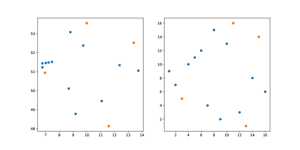
Figure 1: Scatter plot and rank plot for the city data (red: the four largest cities)

3 Patterns, subsampling and convergence

Our aim in this section is to obtain a formal framework for the informal (and ubiquitous) question, ‘what happens as $n\to\infty$?’. We may, for example, start with a sequence $(\pi_{n})_{n\in\mathbb{N}}$ of permutations with $\pi_{n}\in\mathbb{S}_{n}$ for all $n\in\mathbb{N}$ and regard these as elements of the set $\mathbb{S}:=\bigsqcup_{n=1}^{\infty}\mathbb{S}_{n}$, which we then need to augment in order to obtain a limit. A standard procedure begins with a set $\mathcal{F}$ of functions $f:\mathbb{S}\to[0,1]$ that separates the points in the sense that, for each pair $\pi,\sigma\in\mathbb{S}$ with $\pi\not=\sigma$, there is a function $f\in\mathcal{F}$ such that $f(\pi)\not=f(\sigma)$. We then identify $\pi\in\mathbb{S}$ with the function $f\mapsto f(\pi)$, which is an element of the space $[0,1]^{\mathcal{F}}$ which, endowed with the product topology, is compact by Tychonov’s theorem. The closure of the embedded $\mathbb{S}$ provides a compactification $\bar{\mathbb{S}}$ of $\mathbb{S}$, where convergence of a sequence $(\pi_{n})_{n\in\mathbb{N}}$ is equivalent to the convergence of all real sequences $(f(\pi_{n}))_{n\in\mathbb{N}}$, $f\in\mathcal{F}$. Moreover, each function $f\in\mathcal{F}$ has a continuous extension to $\bar{\mathbb{S}}$. In the present situation $\mathcal{F}$ will always be countable, and we start with the discrete topology on $\mathbb{S}$. Then $\bar{\mathbb{S}}$ is a separable compact topological space, and the boundary $\partial\mathbb{S}$ is a compact subset.

We discuss three function classes and the resulting topologies.

First, let $\mathcal{F}$ be the set of indicator functions $f_{\sigma}=1_{\{\sigma\}}$, $\sigma\in\mathbb{S}$, i.e. $f_{\sigma}(\sigma)=1$ and $f_{\sigma}(\pi)=0$ if $\pi\not=\sigma$. Then, if $(\pi_{n})_{n\in\mathbb{N}}$ is a sequence that leaves $\mathbb{S}$ in the sense that for each $k\in\mathbb{N}$ there is an $n_{0}=n_{0}(k)\in\mathbb{N}$ such that $\pi_{n}\notin\mathbb{S}_{k}$ for all $n\geq n_{0}$, we always get the function which is equal to 0 as the pointwise limit, hence the boundary consists of a single point. This topology is known as the one-point compactification.

For the second example we note first that order relations transfer to subsets by restriction. For $A=[n]$, $\pi\in\mathbb{S}_{n}$, and $B=[k]$ with $k\leq n$, restricting $<_{\pi}$ from $A$ to $B$ amounts to deleting all entries greater than $k$ in the one-line notation of $\pi$, which gives the one-line notation for a permutation $\sigma\in\mathbb{S}_{k}$. We generally write $\sigma=\pi[B]$ if $(B,<_{\pi})$ is order isomorphic to $([k],<_{\sigma})$. If $B=\{i_{1},\ldots,i_{k}\}\subset[n]$ with $i_{1}<\cdots<i_{k}$ this is equivalent to

$$\sigma(j)<\sigma(m)\ \Longleftrightarrow\ \pi(i_{j})<\pi(i_{m})\quad\text{for }j,m\in[k],$$

a condition that will appear repeatedly below. We now define $f_{\sigma}:\mathbb{S}\to[0,1]$, $\sigma\in\mathbb{S}_{k}$, by $f_{\sigma}(\pi)=1$ if $\sigma=\pi[A]$ for $A=[k]$, and $f_{\sigma}(\pi)=0$ otherwise. As in the previous case the functions take only the values 0 and 1, so that convergence means that $f_{\sigma}(\pi_{n})$ remains constant from some $n_{0}=n_{0}(\sigma)$ onwards. In view of $\sum_{\sigma\in\mathbb{S}_{k}}f_{\sigma}(\pi)=1$ for all $\pi\in\mathbb{S}_{n}$, $n\geq k$, any such sequence leads to a sequence $(\sigma_{k})_{k\in\mathbb{N}}$, $\sigma_{k}\in\mathbb{S}_{k}$, that has the property that $f_{\sigma_{k}}(\pi_{n})=1$ for all $n\geq n_{0}(k)$. Clearly, this sequence must be projective in the sense that the restriction of $\sigma_{k}$ to $[l]$ with $l\leq k$ is equal to $\sigma_{l}$. This implies that there is a total order $<_{\pi_{\infty}}$ on $\mathbb{N}$ which reduces to $<_{\sigma_{k}}$ on $[k]$ for all $k\in\mathbb{N}$. The result is known as the projective topology, and the set of limits is the set of total orders on $\mathbb{N}$.

The third topology will lead to permutons. It arises if we use pattern counting, another aspect that is closely related to the interpretation of permutations as connecting total orders. Let $M(k,n)$ be the set of strictly increasing functions $f:[k]\to[n]$, $n\geq k$. We define the relative frequency of the pattern $\sigma$ in the permutation $\pi$ as

$$t(\sigma,\pi)\,=\,\frac{1}{\#M(k,n)}\,\#\bigl{\{}f\in M(k,n):\,\sigma(i)<\sigma(j)\,\Leftrightarrow\,\pi(f(i))<\pi(f(j))\bigr{\}}.$$

Of course, $\#M(k,n)=\binom{n}{k}$. We augment this by putting $t(\sigma,\pi)=0$ if $k>n$. Using the notation from the previous paragraph and identifying $f\in M(n,k)$ with its range $A$ we see that the numerator is the number of size $k$ subsets $A$ of $[n]$ with $\pi[A]=\sigma$. Table 1 contains the absolute and relative frequencies for the six patterns of length three in the city data introduced at the end of Section 1. The four largest cities generate the pattern $\sigma=2413\in\mathbb{S}_{4}$.

permutation	123	132	213	231	312	321
pattern frequency	69	57	88	61	130	50
relative frequency	.152	.125	.193	.134	.286	.110

Table 1: Patterns in the city data permutation

From a probabilistic or, in fact, statistical point of view, we may regard the relative frequencies as probabilities in a sampling experiment. With $\xi=\xi_{n,k}$ uniformly distributed on the set of all subsets $A$ of $[n]$ with size $k$, the function $\sigma\mapsto t(\sigma,\pi)$ is the probability mass function of the random element $\pi[\xi]$ of $\mathbb{S}_{k}$. In particular, whenever $k\leq n$,

$$\sum_{\sigma\in\mathbb{S}_{k}}t(\sigma,\pi)\,=\,1\quad\text{for all }\pi\in\mathbb{S}_{n}.$$ (8)

Building on an earlier approach in graph theory, Hoppen et al (2013) introduced a notion of convergence based on such pattern frequencies. We identify a permutation $\pi$ with its function $\sigma\to t(\sigma,\pi)$ on the set $\mathbb{S}$ and with values in the unit interval; it is easy to see that different permutations lead to different functions. The general approach outlined above then leads us to define convergence of the sequence $(\pi_{n})_{n\in\mathbb{N}}$ as convergence of $t(\sigma,\pi_{n})$ for all $\sigma\in\mathbb{S}$. Below we will refer to this as the pattern frequency topology,

For the construction to be of use we need a description of the boundary $\partial\mathbb{S}=\bar{\mathbb{S}}\setminus\mathbb{S}$. In the general setup the limit of a convergent sequence $(\pi_{n})_{n\in\mathbb{N}}$ with $|\pi_{n}|\to\infty$ is simply the function

$$\pi_{\infty}:\mathbb{S}\to[0,1],\quad\sigma\mapsto\lim_{n\to\infty}t(\sigma,\pi_{n}),$$

but obviously, not all functions from $\mathbb{S}$ to $[0,1]$ appear in that manner. For example, (8) implies that $\sum_{\sigma\in\mathbb{S}_{k}}\pi_{\infty}(\sigma)=1$ for any fixed $k\in\mathbb{N}$, and a conditioning argument leads to the inequality $\pi_{\infty}(\sigma)\geq t(\sigma,\rho)\cdot\pi_{\infty}(\rho)$ for all $\sigma\in\mathbb{S}_{k}$, $\rho\in\mathbb{S}_{n}$ with $k\leq n$. In fact, we even have, for all $k,l,m\in\mathbb{N}$ with $k<l<m$ and all $\sigma\in\mathbb{S}_{k}$, $\rho\in\mathbb{S}_{m}$,

$$t(\sigma,\rho)\,=\,\sum_{\tau\in\mathbb{S}_{l}}t(\sigma,\tau)\,t(\tau,\rho).$$ (9)

This follows from viewing the sampling procedure as removing single elements repeatedly, and then decomposing with respect to the permutation obtained at the intermediate level. The decomposition (9) will play an important role later in the context of the dynamics of permutation sequences; see Section 4.

Now copulas enter the stage: A (two-dimensional) copula $C:[0,1]\times[0,1]\to[0,1]$ is the distribution function of a probability measure on the unit square that has uniform marginals, meaning that $C(u,1)=u$ for all $u\in[0,1]$ and $C(1,v)=v$ for all $v\in[0,1]$. We define the associated pattern frequency function $t(\cdot,C)$ by sampling: For $\sigma\in\mathbb{S}_{k}$ let $t(\sigma,C)$ be the probability that a sample $(X_{1},Y_{1}),\ldots,(X_{k},Y_{k})$ from $C$ leads to the permutation $\sigma$ in the sense that

$$\Pi_{n}((X_{1},Y_{1}),\ldots,(X_{k},Y_{k}))=\sigma,$$

see also (5). As the joint distribution of the sample is invariant under permutations it follows that, for all $k\in\mathbb{N}$ and $\sigma\in\mathbb{S}_{k}$,

$$t(\sigma,C)\;=\;k!\,P(X_{1}<X_{2}<\cdots<X_{k},\,Y_{\sigma(1)}<Y_{\sigma(2)}<\cdots<Y_{\sigma(k)}).$$

We observe (but do not prove) that $C$ is determined by the function $\sigma\mapsto t(\sigma,C)$ on $\mathbb{S}$, and that for copulas, weak convergence is equivalent to the pointwise convergence on $\mathbb{S}$ of these functions. Note the analogy to the moment problem in the first and to the moment method in the second statement.

We can now collect and rephrase some of the main results in Hoppen et al (2013). For the definition of the random permutations in part (c) we refer to (5) again, and to the description given there of a suitable algorithm for obtaining the permutation from the data. Ties in the $X$- resp. $Y$-values may be ignored as these are, individually, a sample from the uniform distribution on the unit interval.

Theorem 3.1.

(a) A sequence $(\pi_{n})_{n\in\mathbb{N}}$ of permutations in $\mathbb{S}$ with $|\pi_{n}|\to\infty$ converges in the pattern frequency topology if and only if there is a copula $C$ such that

$$\lim_{n\to\infty}t(\sigma,\pi_{n})=t(\sigma,C)\quad\text{for all }\sigma\in\mathbb{S}.$$ (10)

Moreover, the copula $C$ is unique.

(b) In the pattern frequency topology, the boundary $\partial\mathbb{S}$ is homeomorphic to the space of copulas, endowed with weak convergence.

(c) Let $C$ be a copula and suppose that $(X_{i},Y_{i})$, $i\in\mathbb{N}$, are independent random vectors with distribution function $C$. For each $n\in\mathbb{N}$ let $\Pi_{n}$ be the random permutation associated with the first $n$ pairs $(X_{1},Y_{1}),\ldots,(X_{n},Y_{n})$. Then, in the pattern frequency topology, $\Pi_{n}$ converges to $C$ almost surely as $n\to\infty$.

Below we will refer the stochastic process $(\Pi_{n})_{n\in\mathbb{N}}$ in part (c) of Theorem 3.1 as the permutation sequence generated (or parametrized) by the copula $C$.

From a probabilistic point of view it is not too difficult to understand this result: Let $\mathbb{M}_{1}=\mathbb{M}_{1}([0,1]\times[0,1],\mathcal{B}([0,1]\times[0,1]))$ be the space of probability measures on the Borel subsets of the unit square, endowed with the topology of weak convergence, and consider the embedding $\pi\mapsto\mu(\pi)$ of $\mathbb{S}$ into $\mathbb{M}_{1}$ given by (7). Suppose now that $(\pi_{n})_{n\in\mathbb{N}}$ is a sequence of permutations where we assume for simplicity that $\pi_{n}\in\mathbb{S}_{n}$ for all $n\in\mathbb{N}$. As $\mathbb{M}_{1}$ is compact with respect to weak convergence this sequence has a limit point $\mu_{\infty}$, and convergence would follow from the uniqueness of $\mu_{\infty}$. For this we first note that the marginals of any such limit point are the uniform distributions on the unit interval, as weak convergence implies the convergence of the marginal distributions. Hence any limit point $\mu_{\infty}$ has as its distribution function a copula $C$. Next we argue that (10) holds: Let $\sigma\in\mathbb{S}_{k}$ be given and let the function $h_{\sigma}$ on $([0,1]\times[0,1])^{k}$ indicate whether or not the order-relating permutation for the marginal rank vectors of $((x_{1},y_{1}),\ldots,(x_{k},y_{k}))$ is equal to $\sigma$. Then

$$t(\sigma,\pi_{n})\,=\,\frac{1}{\binom{n}{k}}\sum_{1\leq i_{1}<\cdots<i_{k}\leq n}h_{\sigma}\bigl{(}(x_{i_{1}},y_{i_{1}})\ldots,(x_{i_{k}},y_{i_{k}})\bigr{)}.$$ (11)

Uniform marginals implies that the set of discontinuities of $h_{\sigma}$ is a $\mu_{\infty}$-null set, and the weak convergence of $\mu(\pi_{n})$ to $\mu_{\infty}$ implies the weak convergence of the respective $k$th measure-theoretic powers. Taken together this shows (10). The desired uniqueness now follows from the fact that a copula $C$ is determined by its function $\sigma\to t(\sigma,C)$. For (b) we use that weak convergence of copulas is equivalent to pointwise convergence of the associated functions on $\mathbb{S}$. Finally, part (c) is immediate from the representation (11) of pattern frequencies as $U$-statistics, and the classical consistency result for the latter.

4 Dynamics

Generating random permutations is an important applied task. In line with the history of probability we recall a standard gaming example: Card mixing requires $\Pi_{n}\sim\text{\rm unif}(\mathbb{S}_{n})$ for some fixed $n$. Many shuffling algorithms may be modeled as random walks on $\mathbb{S}_{n}$ and can then be analyzed using the representation theory for this group; see also Section 6.2 below.

Here we are interested in sequences $(\Pi_{n})_{n\in\mathbb{N}}$ with $\Pi_{n}\in\mathbb{S}_{n}$ for all $n\in\mathbb{N}$, and a Markovian dynamic. A classical example is the Markov chain $\Pi^{\tiny\rm F}=(\Pi^{\tiny\rm F}_{n})_{n\in\mathbb{N}}$ which starts at $\Pi^{\tiny\rm F}_{1}\equiv(1)$ and then uses independent random variables $I_{n}\sim\text{\rm unif}([n+1])$, independent of $\Pi^{\tiny\rm F}_{1},\ldots,\Pi^{\tiny\rm F}_{n}$, to construct $\Pi^{\tiny\rm F}_{n+1}$ from $\Pi^{\tiny\rm F}_{n}=(\pi(1),\ldots,\pi(n))$ as follows,

$$\Pi^{F}_{n+1}=\bigl{(}\pi(1),\ldots,\pi(I_{n}-1),n+1,\pi(I_{n}),\ldots,\pi(n)\bigr{)}.$$ (12)

In words: We insert the new value $n+1$ at a position in a gap chosen uniformly at random. This appears, for example, on p.132 in Feller (1968). A second possibility, which we will relate to Hoppen et al (2013), and which we denote by $\Pi^{\tiny\rm H}=(\Pi^{\tiny\rm H}_{n})_{n\in\mathbb{N}}$, uses ‘double insertion’ instead. This means that the step from $n$ to $n+1$ is based on two independent random variables $I=I_{n}$ and $J=J_{n}$, both uniformly distributed on $[n+1]$, and

$$\Pi^{\tiny\rm H}_{n+1}(i)\,=\,\begin{cases}\Pi^{\tiny\rm H}_{n}(i),&\text{if }i<I\text{ and }\Pi^{\tiny\rm H}_{n}(i)<J,\\ \Pi^{\tiny\rm H}_{n}(i)+1,&\text{if }i<I\text{ and }\Pi^{\tiny\rm H}_{n}(i)\geq J,\\ J,&\text{if }i=I,\\ \Pi^{\tiny\rm H}_{n}(i-1),&\text{if }i>I\text{ and }\Pi^{\tiny\rm H}_{n}(i)<J,\\ \Pi^{\tiny\rm H}_{n}(i-1)+1,&\text{if }i>I\text{ and }\Pi^{\tiny\rm H}_{n}(i)\geq J.\end{cases}$$ (13)

In words: We insert $J$ at position $I$ and increase the appropriate values by 1. Obviously, this process is a Markov chain, again with start at the single element $\sigma=(1)$ of $\mathbb{S}_{1}$. We collect some properties of this process. The notion of a permutation sequence generated by a copula is explained in Theorem 3.1 (c).

Lemma 1.

Let $\Pi^{\tiny\rm H}$ be as defined above.

(a) $\ \Pi^{\tiny\rm H}$ is equal in distribution to the permutation sequence generated by the independence copula $C(x,y)=x\cdot y$.

(b) The transition probabilities of $\Pi^{\tiny\rm H}$ are given by

$$p^{\tiny\rm H}(\sigma,\tau):=P(\Pi^{\tiny\rm H}_{n}=\tau|\Pi^{\tiny\rm H}_{k}=\sigma)\,=\,\frac{k!}{n!}\,t(\sigma,\tau)$$ (14)

for all $k,n\in\mathbb{N}$ with $k\leq n$, and all $\sigma\in\mathbb{S}_{k}$ and $\tau\in\mathbb{S}_{n}$.

(c) $\ \Pi^{\tiny\rm H}_{n}\sim\text{\rm unif}(\mathbb{S}_{n})\$ for all $n\in\mathbb{N}$.

Proof:.

(a) Let $\Pi=(\Pi_{n})_{n\in\mathbb{N}}$ be generated by the independence copula. Then the step from $\Pi_{n}$ to $\Pi_{n+1}$ is based on the component ranks $I$ and $J$ of the next pair $(X_{n+1},Y_{n+1})$ in the sequence $(X_{1},Y_{1}),\ldots,(X_{n+1},Y_{n+1})$. It is well known that $I$ and $J$ are both uniformly distributed on $[n+1]$. Here they are also independent, hence $\Pi_{n+1}$ arises from $\Pi_{n}$ as in (13).

(b) The transition from $\sigma\in\mathbb{S}_{n}$ to $\tau\in\mathbb{S}_{n+1}$ is based on independent random variables $I$ and $J$, both uniformly distributed on $[n+1]$. If $I=i$ then, with $\phi_{i}:[n]\to[n+1]$, $\phi_{i}(k)=k$ if $k\leq i$ and $\phi_{i}(k)=k+1$ if $k>i$, we must have $\sigma(l)<\sigma(m)$ if and only if $\tau(\phi_{i}(l))<\tau(\phi_{i}(m))$ for all $l,m\in[n]$. The number of such $i$’s is $(n+1)\,t(\sigma,\tau)$, and in each case we additionally need $J=\tau(I)$. This proves the one-step version of (14).

To obtain the general case we now use induction, the Markov property, and (9).

(c) This is immediate from (14) with $k=1$ and $\sigma=1$. ∎

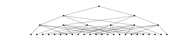
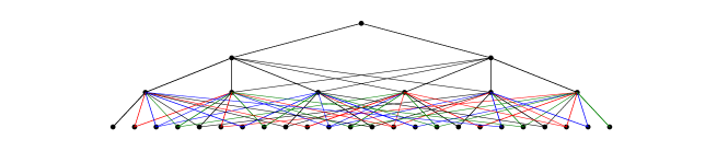
Figure 2: The transition graphs for the Markov chains $\Pi^{\tiny\rm F}$ (top) and $\Pi^{\tiny\rm H}$ (bottom)

Hence both $\Pi^{\tiny\rm F}$ and $\Pi^{\tiny\rm H}$ consist of uniformly distributed variables. A trivial third possibility to achieve this is to use independent $\Pi_{n}$’s with $\Pi_{n}\sim\text{\rm unif}(\mathbb{S}_{n})$. The transition graph for these chains has $\mathbb{S}$ as its set of nodes and an edge $\{\sigma,\tau\}$ for each pair $\sigma\in\mathbb{S}_{n}$, $\tau\in\mathbb{S}_{n+1}$, $n\in\mathbb{N}$, with the property that $P(\Pi_{n+1}=\tau|\Pi_{n}=\sigma)>0$. Figure 2 shows the first four levels of the transition graphs for $\Pi^{\tiny\rm F}$ and $\Pi^{\tiny\rm H}$. These graphs are the Hasse diagrams associated with two specific partial orders on $\mathbb{S}$. In the first, $\sigma<_{\text{\tiny{F}}}\rho$ for $\sigma\in\mathbb{S}_{k}$ and $\rho\in\mathbb{S}_{n}$ with $k<n$ means that the one-line notation for $\sigma$ arises from the one-line notation for $\rho$ by simply deleting all values greater than $k$ in the latter, whereas in connection with $\Pi^{\tiny\rm H}$ we have $\sigma<_{\text{\tiny{H}}}\rho$ if and only if $\sigma$ appears as a pattern in $\rho$. Clearly, the graph for $\Pi^{\tiny\rm F}$ is a tree: All previous states are deterministic functions of the current state. Informally speaking, all three chains eventually leave the state space $\mathbb{S}$, and this is what provides the connection to the previous section.

We need an excursion. The Markov property is often stated informally as ‘the future development depends on the history of the process only via its present state’. It may be instructive to carry out a simple calculation: If $X_{1},X_{2},\ldots,X_{n}$ are random variables on some probability space with values in some countable set, then their joint distribution can always be evaluated step by step via

$$P(X_{1}=x_{1},\ldots,X_{n}=x_{n})\;=\;P(X_{1}=x_{1})\cdot\prod_{i=2}^{n}P(X_{i}=x_{i}|X_{i-1}=x_{i-1},\ldots,X_{1}=x_{1}),$$

whenever the probability on the left hand side is positive. If the tuple has the Markov property then elementary manipulations of conditional probabilities lead to

$$P(X_{1}=x_{1},\ldots,X_{n}=x_{n})\ =\ P(X_{1}=x_{1})\cdot\,\prod_{i=2}^{n}P(X_{i}=x_{i}|X_{i-1}=x_{i-1})$$

$$=\ P(X_{1}=x_{1})\cdot\prod_{i=2}^{n}P(X_{i-1}=x_{i-1}|X_{i}=x_{i})\,\frac{P(X_{i}=x_{i})}{P(X_{i-1}=x_{i-1})}$$

$$=\ P(X_{n}=x_{n})\prod_{i=n-1}^{1}P(X_{i}=x_{i}|X_{i+1}=x_{i+1}).$$

Hence the Markov property then also holds ‘in the other direction’. Moreover, the converse statement follows on reading the above from bottom to top. For a sequence $(X_{n})_{n\in\mathbb{N}}$, and with $\mathcal{G}_{n},\mathcal{H}_{n}$ the $\sigma$-fields generated by the variables $X_{1},\ldots,X_{n}$ and $X_{n},X_{n+1},\ldots$ respectively, the Markov property can formally be written as $\mathcal{L}(X_{n+1}|\mathcal{G}_{n})=\mathcal{L}(X_{n+1}|X_{n})$, $n\in\mathbb{N}$, and the above argument shows that this implies $\mathcal{L}(X_{n-1}|\mathcal{H}_{n})=\mathcal{L}(X_{n-1}|X_{n})$, $n\in\mathbb{N}$, a procedure that may be interpreted as time reversal. In fact, a somewhat neutral statement would be that, for a Markov process, past and future are conditionally independent, given the present.

The distribution of a Markov chain is specified by the distribution of the first variable and the (forward) transition probabilities; for the reverse chain we speak of the cotransition probabilities. The tree structure of its transition graph implies that for $\Pi^{\tiny\rm F}$ the cotransitions are degenerate in the sense only the values 0 and 1 occur. For $\Pi^{\tiny\rm H}$ we use Lemma 1 to obtain

$$P(\Pi^{\tiny\rm H}_{n}=\sigma|\Pi^{\tiny\rm H}_{n+1}=\tau)\ =\ \frac{P(\Pi^{\tiny\rm H}_{n}=\sigma)}{P(\Pi^{\tiny\rm H}_{n+1}=\tau)}\,p^{\tiny\rm H}(\sigma,\tau)\ =\ t(\sigma,\tau)$$ (15)

for all $n\in\mathbb{N}$, $\sigma\in\mathbb{S}_{n}$ and $\tau\in\mathbb{S}_{n+1}$. The decomposition (9) can now be interpreted as describing the backwards movement of $\Pi^{\tiny\rm H}$: Pattern frequencies arise as cotransitions for this chain.

Next we sketch Markov chain boundary theory, which grew out of the historically very important probabilistic approach to classical potential theory. For the highly transient chains considered here, where no state can be visited twice and where the time parameter is a function of the state and thus time homogeneity is implicit, this takes on a particularly simple form. Suppose that $X=(X_{n})_{n\in\mathbb{N}}$ is a Markov chain with graded state space $S=\bigsqcup S_{n}$, that $X$ is adapted to the grading in the sense that $X_{n}\in S_{n}$ for all $n\in\mathbb{N}$, and that $S$ is minimal in the sense that $P(X_{n}=x)>0$ for all $x\in S_{n}$, $n\in\mathbb{N}$. The Martin kernel $K:S\times S\to\mathbb{R}_{+}$ for $X$ is then given by

$$K(x,y)\,:=\,\frac{P(X_{n}=y|X_{m}=x)}{P(X_{n}=y)}\quad\text{for all }x\in S_{m},\,y\in S_{n}$$ (16)

if $n\geq m$, and $K(x,y)=0$ otherwise. For each $x\in S_{m}$ let $f_{x}:S\to[0,1]$ be defined by

$$f_{x}(y)\,=\,P(X_{m}=x)\,K(x,y)\,=\,P(X_{m}=x|X_{n}=y)$$ (17)

and let $\mathcal{F}:=\{f_{x}:\,x\in S\}$. The Doob-Martin compactification $\bar{S}$ and the Martin boundary $\partial S$ of the state space are the results of the procedure outlined at the beginning of Section 3, with this choice of $\mathcal{F}$ as space of separating functions.

We give two central results.

Theorem 4.1.

In the Doob-Martin compactification, $X_{n}$ converges almost surely to a random variable $X_{\infty}$ with values in the Martin boundary.

Proof:.

Let $f=f_{x}\in\mathcal{F}$ with some $x\in S_{k}$. In view of the above remarks on the Markov property and time reversal,

$$f(X_{n})\,=\,P(X_{k}=x|X_{n})\,=\,E[1_{\{x\}}(X_{k})|\mathcal{H}_{n}]\quad\text{for all }n\geq k,$$

so that, as $\mathcal{H}_{n+1}\subset\mathcal{H}_{n}$,

$$E[f(X_{n})|\mathcal{H}_{n+1}]\,=\,E\bigl{[}E[1_{\{x\}}(X_{k})|\mathcal{H}_{n}]\big{|}\mathcal{H}_{n+1}\bigr{]}\,=\,E[1_{\{x\}}(X_{k})|\mathcal{H}_{n+1}]\,=\,f(X_{n+1}).$$

This shows that $\bigl{(}f(X_{n}),\mathcal{H}_{n}\bigr{)}_{n\geq k}$ is a reverse martingale, hence $f(X_{n})$ converges almost surely. As $x\in S$ was arbitrary, the first statement follows by construction of the compactification.

As $P(X_{\infty}\in\bigcup_{k=1}^{n}S_{k})=0$ for all $n\in\mathbb{N}$, we also get $P(X_{\infty}\in\partial S)=1$. ∎

The general compactification procedure implies that the Martin kernel can be extended continuously from $S\times S$ to $S\times\bar{S}$ via $K(x,\alpha)=\lim_{n\in\mathbb{N}}K(x,y_{n})$ where $(y_{n})_{n\in\mathbb{N}}$ is such that $y_{n}\to\alpha\in\partial S$ in the Doob-Martin topology. The following is a special case of Doob’s $h$-transform.

Theorem 4.2.

Let $X,S,\bar{S},\partial S$ be as above and let $p(x,y)=P(X_{n+1}=y|X_{n}=x)$, $x\in S_{n}$, $y\in S_{n+1}$, be the transition function of the Markov chain $X$. For $\alpha\in\partial S$ let $p^{\alpha}$ be defined by

$$p^{\alpha}(x,y)\,=\,\frac{K(y,\alpha)}{K(x,\alpha)}\,p(x,y)\quad\text{for all }n\in\mathbb{N},\;x\in S_{n},\,y\in S_{n+1}.$$

Then $p_{\alpha}$ is the transition function for a Markov chain $X^{\alpha}=(X^{\alpha}_{n})_{n\in\mathbb{N}}$, and $X^{\alpha}_{n}$ converges almost surely to $\alpha$ in the Doob-Martin topology.

The picture that emerges from these results is that of an exit boundary and, with $K(\cdot,\alpha)$ as basis for an $h$-transform, of the resulting transformed chain as the process conditioned on the value $\alpha\in\partial S$ for the limit $X_{\infty}$. Further, the relation to time reversal and the two-sidedness of the Markov property outlined above shows that convergence $y_{n}\to\alpha\in\partial S$ in the Doob-Martin topology is equivalent to the convergence in distribution of the initial segments of the conditioned chain,

$$\mathcal{L}[X_{1},\ldots,X_{k}|X_{n}=y_{n}]\;\to_{\text{\rm\tiny distr}}\;\mathcal{L}[X_{1},\ldots,X_{k}|X_{\infty}=\alpha]\quad\text{for all }k\in\mathbb{N}.$$

Finally, we note that the topological construction depends on the chain via the associated cotransitions only. In the familiar forward case, the distribution of $X$ is specified by the distribution of the first variable $X_{1}$ and the transition function $p$. Here we may consider the distribution of $X_{\infty}$ as given, and then use the cotransitions to obtain the distribution of $X$ as a mixture of the distributions $\mathcal{L}[X|X_{\infty}=\alpha]$, $\alpha\in\partial S$.

We now return to processes $(\Pi_{n})_{n\in\mathbb{N}}$ of permutations. This is a special case of the above framework, with $S=\mathbb{S}$ and $S_{n}=\mathbb{S}_{n}$. First, for $\Pi^{\tiny\rm F}$ it is clear from the transition mechanism that, for $\sigma\in\mathbb{S}_{k}$ and $\pi\in\mathbb{S}_{n}$, the conditional probability $P(\Pi^{\tiny\rm F}_{k}=\sigma|\Pi^{\tiny\rm F}_{n}=\pi)$ has value 1 if the (order) restriction of $\pi$ to $[k]$ is equal to $\sigma$, and that it is 0 otherwise. As functions on $\mathbb{S}$ these are the same as the functions that generate the projective topology, see Section 3. Of course, convergence in the projective topology also follows directly from the fact that $\Pi^{\tiny\rm F}$ is consistent in the sense that, for all $n\in\mathbb{N}$, the restriction of $\Pi^{\tiny\rm F}_{n+1}$ to $[n]$ is equal to $\Pi^{\tiny\rm F}_{n}$. At the other end of the spectrum, with the chain consisting of independent random variables, we obtain the one-point compactification, where each sequence of permutations that does not have a limit point in $\mathbb{S}$ itself converges to the single point $\infty$. An intermediate case is $\Pi^{\tiny\rm H}$ or, more generally, the copula-based process introduced in part (c) of Theorem 3.1. Recall that $\Pi^{\tiny\rm H}$ appears with the independence copula $C(x,y)=x\cdot y$.

Theorem 4.3.

The process $\Pi=(\Pi_{n})_{n\in\mathbb{N}}$ generated by a copula $C$ is a Markov chain with transition probabilities

$$P(\Pi_{n+1}=\tau|\Pi_{n}=\sigma)\,=\,\frac{(n+1)\,t(\tau,C)}{t(\sigma,C)}\,p^{\tiny\rm H}(\sigma,\tau),\quad n\in\mathbb{N},\,\sigma\in\mathbb{S}_{n},\tau\in\mathbb{S}_{n+1},$$ (18)

and the associated Doob-Martin topology is the same as the pattern frequency topology. Further, $\Pi$ is an $h$-transform of $\Pi^{\tiny\rm H}$.

Proof:.

We consider $\Pi^{\tiny\rm H}$ first. By (15) the functions in (17) evaluate to $f_{\sigma}(\pi)=t(\sigma,\pi)$, which implies that the Doob-Martin topology coincides with the pattern frequency topology.

For an arbitrary copula $C$ the permutations are generated by a sequence of independent random vectors $(X_{i},Y_{i})$, $i\in\mathbb{N}$, with distribution function $C$, and $\Pi_{n}$ is a deterministic function of the first $n$ pairs. The conditional distribution of $\Pi_{n}$ given all $\Pi_{k}$, $k>n$, thus depends only on $\Pi_{n+1}$ and the pair $(i,j)$ in the permutation plot of $\Pi_{n+1}$ that has been generated by $(X_{n+1},Y_{n+1})$. As the initial segments are invariant in distribution under permutations, each $i\in[n+1]$ is equally likely. Taken together this shows that $(\Pi_{n})_{n\in\mathbb{N}}$ is a Markov chain with cotransitions that do not depend on $C$. This completes the proof of the topological assertion.

In order to obtain the expression for the one-step transition probabilities we note that, by definition of $t(\cdot,C)$,

$$P(\Pi_{k}=\sigma)\,=\,t(\sigma,C)\quad\text{for all }k\in\mathbb{N},\,\sigma\in\mathbb{S}_{k}.$$

Using this together with (14), (15) and some elementary manipulations leads to (18).

For the proof of the last assertion we need the extended Martin kernel $K(\cdot,\cdot)$ associated with $\Pi^{\tiny\rm H}$. First, by the familiar arguments,

$$K(\sigma,\pi)\,=\,\frac{P(\Pi^{\tiny\rm H}_{k}=\sigma|\Pi^{\tiny\rm H}_{n}=\pi)}{P(\Pi^{\tiny\rm H}_{k}=\sigma)}\;=\;k!\,t(\sigma,\pi)$$

for all $\sigma\in\mathbb{S}_{k},\pi\in\mathbb{S}_{n}$ with $k\geq n$. Suppose now that $(\pi_{n})_{n\in\mathbb{S}}$ is such that $\pi_{n}\to C\in\partial\mathbb{S}$. As the extension of $K(\sigma,\cdot)$ to $\bar{\mathbb{S}}$ is continuous, it follows that

$$K(\sigma,C)\,=\,\lim_{n\to\infty}K(\sigma,\pi_{n})\,=\,k!\lim_{n\to\infty}t(\sigma,\pi_{n})\,=\,k!\;t(\sigma,C),$$

where we have used Theorem 3.1 (a) in the last step. Using this (18) can be written as

$$P(\Pi_{n+1}=\tau|\Pi_{n}=\sigma)\,=\,\frac{K(\tau,C)}{K(\sigma,C)}\,P\bigl{(}\Pi^{\tiny\rm H}_{n+1}=\tau|\Pi^{\tiny\rm H}_{n}=\sigma\bigr{)}$$

for all $n\in\mathbb{N}$, $\sigma\in\mathbb{S}_{n}$ and $\tau\in\mathbb{S}_{n+1}$. ∎

We presented a purely topological approach to state space augmentation that is based on an embedding of $\mathbb{S}$ into $[0,1]^{\mathcal{F}}$ with a suitable family $\mathcal{F}$ of functions $f:\mathbb{S}\to[0,1]$ and the subsequent use of Tychonov’s theorem. This is a variant of the famous Stone-Čech compactification; see e.g. (Kelley, 1955, p.152). Alternatively, we could endow $\mathbb{S}$ with a metric $d$ and then pass to the completion of $(\mathbb{S},d)$. A suitable choice of $d$, based on the Martin kernel, leads to a totally bounded metric space that is topologically homeomorphic to the compactification discussed above.

5 Applications

We give a range of examples where permutations and their limits are important, from classical statistics to stochastic modeling to theoretical computer science.

5.1 Tests for independence

If the $X$- and $Y$-variables are independent then we obtain the copula $C(x,y)=x\cdot y$, $0\leq x,y\leq 1$. For the asymptotic frequencies this means that, for all $k\in\mathbb{N}$ and $\sigma\in\mathbb{S}_{k}$,

$$t(\sigma,C)\ =\ k!\,P(X_{1}<X_{2}<\ldots<X_{k},\,Y_{1}<Y_{2}<\ldots<Y_{k}),$$

as a permutation of the $Y$-variables alone does not change the joint distribution of the pairs $(X_{1},Y_{1}),\ldots,(X_{n},Y_{n})$. In particular, all patterns of the same length have the same asymptotic frequencies, so that $\,t(\sigma,C)=1/k!\,$ for all $\sigma\in\mathbb{S}_{k}$.

This may be used for testing independence. A famous classical procedure is based on Kendall’s $\tau$-statistic which, in the notation introduced in Section 3, may be written as $\tau=\bigl{(}t(12,\Pi_{n})-t(21,\Pi_{n})\bigr{)}/\binom{n}{2}$ and thus makes use of the two complementary patterns of length two. A central limit theorem for $U$-statistics leads to a test for independence with asymptotically correct level, see e.g. Example 12.5 in van der Vaart (1998). In our running data example a total of 61 of the 120 pairs are concurrent: Clearly, the test based on Kendall’s $\tau$ would not reject the hypothesis of independence for these data.

An analogous procedure based on longer patterns requires a multivariate central limit theorem for vectors of $U$-statistics. We consider patterns of length three, with a view towards the values given in Table 1. For the asymptotic covariances we use Theorem 12.3 in van der Vaart (1998) and thus have to compute $\zeta(\sigma,\tau):=3^{2}\,\text{\rm cov}(h_{\sigma}(Z_{1},Z_{2},Z_{3}),h_{\tau}(Z_{1},Z^{\prime}_{2},Z^{\prime}_{3}))$ for $\sigma,\tau\in\mathbb{S}_{3}$, where $Z_{1},Z_{2},Z_{3},Z^{\prime}_{2},Z^{\prime}_{3}$ are independent and uniformly distributed on the unit square. For this we first determine the conditional distribution $\mathcal{L}[\Pi_{3}|X_{1}=x,Y_{1}=y]$ under the assumption of independence of horizontal and vertical positions. If $\pi=123$, for example, we either have $X_{2}<x,Y_{2}<y,X_{3}>x,Y_{3}>y$ or $X_{3}<x,Y_{3}<y,X_{2}>x,Y_{2}>y$ if $(x,y)$ is ‘in the middle’ of the rank plot, and similar conditions apply in the other two cases. With $\phi_{\sigma}(x,y):=P(\Pi_{3}=\sigma|X_{1}=x,Y_{1}=y)$ elementary calculations along these lines lead to

$$\phi_{123}(x,y)\; =\;2x(1-x)y(1-y)+x^{2}y^{2}/2+(1-x)^{2}(1-y)^{2}/2,$$

$$\phi_{132}(x,y)\; =\;x^{2}y(1-y)+x(1-x)y^{2}+(1-x)^{2}(1-y)^{2}/2,$$

$$\phi_{213}(x,y)\; =\;x(1-x)(1-y)^{2}+(1-x)^{2}y(1-y)+x^{2}y^{2}/2,$$

$$\phi_{231}(x,y)\; =\;x(1-x)y^{2}+(1-x)^{2}y(1-y)+x^{2}(1-y)^{2}/2,$$

$$\phi_{312}(x,y)\; =\;x(1-x)(1-y)^{2}+x^{2}y(1-y)+(1-x)^{2}y^{2}/2,$$

$$\phi_{321}(x,y)\; =\;2x(1-x)y(1-y)+x^{2}(1-y)^{2}/2+(1-x)^{2}y^{2}/2.$$

Note that $\phi_{\sigma}(x,y)=\phi_{\sigma^{-1}}(y,x)$ for all $\sigma\in\mathbb{S}$, $0<x,y<1$. With these conditional probabilities we get

cov $$(h_{\sigma}(Z_{1},Z_{2},Z_{3}),h_{\tau}(Z_{1},Z^{\prime}_{2},Z^{\prime}_{3}))$$

$$=\ E\bigl{(}h_{\sigma}(Z_{1},Z_{2},Z_{3})h_{\tau}(Z_{1},Z_{2}^{\prime},Z_{3}^{\prime})\bigr{)}\;-\;\bigl{(}Eh_{\sigma}(Z_{1},Z_{2},Z_{3})\bigr{)}\bigl{(}Eh_{\tau}(Z_{1},Z_{2},Z_{3})\bigr{)}$$

$$=\ \int_{0}^{1}\!\!\int_{0}^{1}\phi_{\sigma}(x,y)\phi_{\tau}(x,y)\,dx\,dy\;-\;\Bigl{(}\int_{0}^{1}\!\!\int_{0}^{1}\phi_{\sigma}(x,y)\,dx\,dy\Bigr{)}\Bigl{(}\int_{0}^{1}\!\!\int_{0}^{1}\phi_{\tau}(x,y)\,dx\,dy\Bigr{)}.$$

The observed value 0.228 for $\sigma=312$ deviates notably from the theoretical $1/6$. For this permutation the asymptotic variance is $\zeta=9(19/600-1/36)=7/200$. The corresponding asymptotic $p$-value for the observation would be the probability that a standard normal variable exceeds the value

$$\sqrt{16}\,\sqrt{\frac{200}{7}}\,\biggl{(}0.228-\frac{1}{6}\biggr{)}\ \approx\ 1.311,$$

which is about $0.094$ and thus significant at the level $0.1$. This, of course, is an act of ‘data snooping’, but it should be clear from the above how to obtain the $6\times 6$ asymptotic covariance matrix for the vector $(t(\sigma,\Pi_{n}))_{\sigma\in\mathbb{S}_{3}}$ of pattern frequencies under the hypothesis of independence, and how then to apply an appropriate test with the full data set in Table 1.

The use of ever longer patterns is a straightforward if computationally demanding generalization. In this context another interesting connection between discrete mathematics and statistics appears: A (deterministic) sequence $(\pi_{n})_{n\in\mathbb{N}}$ of permutations with $|\pi_{n}|\to\infty$ is said to be quasirandom if $t(\sigma,\pi_{n})$ converges to $1/|\sigma|!$ for all $\sigma\in\mathbb{S}$. The (random) sequence $(\Pi_{n})_{n\in\mathbb{N}}$ generated by the independence copula has this property with probability one, so such sequences exist (there is an obvious parallel with normal numbers). Is it enough for quasirandomness if the limit statement holds for all permutations of some fixed length $k$? It follows from (9) that this ‘forcing property’ would then automatically hold for all $j\geq k$ and, clearly, $k=2$ is too small. This question has been answered in Král and Pikhurko (2013), who showed that quasiramdomness follows with $k=4$, but not with $k=3$. Their proof of the sufficiency part is based on the permuton approach discussed in Section 3. In fact, as every limit point $C$ must satisfy $t(\sigma,C)=1/4!$ for all $\sigma\in\mathbb{S}_{4}$, the statement boils down to a characterization property of the independence copula. Remarkably, in a statistical context, such a characterization had been obtained much earlier in Yanagimoto (1970), and it leads to an extension of Kendall’s $\tau$ that is consistent against all alternatives. In both areas, related questions are active fields of research. In connection with quasirandomness we refer to Crudele et al (2023), for the statistical side see e.g. Shi et al (2022).

5.2 Delay models

Objects arrive at a system at times $U_{1},U_{2},\ldots$ and leave at times $U_{1}+X_{1},U_{2}+X_{2},\ldots$, where we assume that the arrivals are independent and uniformly distributed on the unit interval, that the delay times are independent with distribution function $G$, and that arrival and delay times are independent. Let $\Pi_{n}$ be the random permutation that connects the orders of the first $n$ arrivals and departures. For example, in a queuing context, arriving customers might receive consecutively numbered tickets which they return on departure, and the tickets are put on a stack.

In Baringhaus and Grübel (2022) the resulting permutons, the delay copulas, are discussed. From a probabilistic and statistical point of view the information about the delay distribution contained in the permutations is of interest, together with the question of how to estimate (aspects of) the delay distribution. Another point of interest are second order approximations or, in general terms, the transitions from a strong law of large number to a central limit theorem. For the set of patterns of a fixed size this has already been important in Section 5.1. In Baringhaus and Grübel (2022) this is taken further by considering $\sqrt{n}(\Pi_{n}(\sigma)-t(\sigma,C))_{\sigma\in\mathbb{S}}$ as a stochastic process with $\sigma\in\mathbb{S}$ as ‘time parameter’ and then establishing a functional central limit theorem.

5.3 Sparseness

The delay models considered in Section 5.2 can be related to the $M/G/\infty$ queue where customers arrive at the times of a Poisson process with intensity $\lambda$. There are infinitely many servers so, strictly speaking, there is no queuing. The limits refer to an increasing arrival rate and thus generate a ’dense’ sequence of permutations as the service time distribution is kept fixed. Here we regard the standard $M/G/1$ model with only one server and fixed arrival rate; for convenience we start with an empty queue at time 0. From the first $n\in\mathbb{N}$ arrivals and departures we still obtain a sequence $(\Pi_{n})_{n\in\mathbb{N}}$ of random permutations, with $\Pi_{n}\in\mathbb{S}_{n}$ for all $n\in\mathbb{N}$. We argue that this sequence is ‘sparse’, and that the pattern frequency topology does not provide much insight.

We assume that the service time distribution has finite first moment $\mu$ and that $\rho<1$, where $\rho:=\lambda\mu$ is known as the traffic intensity. The queue is then stable and the queue length process $Q=(Q_{t})_{t\geq 0}$, with $Q_{t}$ the number of customers in the system at time $t$, can be decomposed into alternating busy and idle periods. These are independent, and the individual sequences of busy and idle pieces of $Q$ are identically distributed. Obviously, arrival and departure times of any particular customer belong to the same busy period. Let $K_{i}$ be the number of customers in the $i$th period. We recall the definition of the direct sum of finite permutations: For $\sigma\in\mathbb{S}_{k}$, $\tau\in\mathbb{S}_{l}$, we obtain the sum $\sigma\oplus\tau\in\mathbb{S}_{l+k}$ in one-line notation as

$$\sigma\oplus\tau=(\sigma_{1},\sigma_{2},\ldots,\sigma_{k},\tau_{1}+k,\tau_{2}+k,\ldots,\tau_{l}+k).$$

Suppose now that $K_{1}=k$. Then, for all $n\geq k$, $\Pi_{n}(i)\leq k$ if $i\leq k$, and $\Pi_{n}(i)>k$ if $k<i\leq n$, hence $\Pi_{n}=\sigma\oplus\tau$ with some $\sigma\in\mathbb{S}_{k}$. Iterating this argument we see that, as $n\to\infty$, $\Pi_{n}$ decomposes into subpermutations related to the sequence of busy cycles. Also, for any given $i$, $\Pi_{n}(i)$ remains constant as soon as $n$ exceeds the number of the first customer no longer in the same busy period as customer $i$. Taken together this leads to the following result.

Proposition 1.

Let $(\Pi_{n})_{n\in\mathbb{N}}$ be the sequence of permutations generated by an $M/G/1$ queue with traffic intensity $\rho<1$. Then $\ \Pi_{n}\to\Pi_{\infty}$ almost surely in the projective topology, with $\;\Pi_{\infty}=_{\text{\rm\tiny distr}}\bigoplus_{i=1}^{\infty}\Psi_{i}$, where $\Psi_{i}\in\mathbb{S}$, $i\in\mathbb{N}$, are independent and identically distributed and $|\Psi_{i}|=K_{i}$.

The distribution $\mathcal{L}(\Pi_{\infty})$ of the limit $\Pi_{\infty}$ is fully characterized by $\mathcal{L}(\Psi_{1})$, which may in turn be specified by $\mathcal{L}(K_{1})$ and the conditional distribution $\mathcal{L}(\Psi_{1}|K_{1})$. Nothing is known (to me) about the latter, apart from the obvious fact that it is concentrated on the subset of $\mathbb{S}_{K_{1}}$ of permutations that cannot be written as a direct sum.

The sequence $(\Pi_{n})_{n\in\mathbb{N}}$ in Proposition 1 is contained in the compactification of $\mathbb{S}$ that we used in the ‘dense’ situation. Under a mild moment condition we obtain the corresponding set of limit points.

Proposition 2.

Suppose that, in addition to the assumptions in Proposition 1, the service time distribution has finite third moment. Then, in the pattern frequency topology, $\Pi_{n}\to C_{\infty}$ almost surely, where the permuton $C_{\infty}$ is given by $C_{\infty}(u,v)=\min\{u,v\}$ for all $u,v\in[0,1]$.

Proof:.

The path-wise argument used for Proposition 1 shows that for any pair $(i,j)$ with $i<j$ and $\Pi_{n}(i)>\Pi_{n}(j)$ customers $i$ and $j$ must belong to the same busy period. In particular,

$$\#\bigl{\{}1\leq i<j\leq n:\,\Pi_{n}(i)>\Pi_{n}(j)\bigr{\}}\,\leq\,n\,M_{n},\quad\text{with }M_{n}:=\max\{K_{1},\ldots,K_{n}\},$$

so that the relative frequency of the inversion $\tau=21$ satisfies $t(\tau,\Pi_{n})\leq 2\,M_{n}/(n-1)$. It follows from Section 5.6, p158 in Cox and Smith (1961) that $EK_{1}^{3}<\infty$ under the above moment assumption. By a standard argument this implies $M_{n}/n\to 0$ almost surely.

Now let $\sigma$ be a permutation that contains an inversion. The relative frequency $t(\sigma,\pi)$ of $\sigma$ in $\pi\in\mathbb{S}_{n}$, $n\geq k:=|\sigma|$, can be interpreted as the probability that $\pi[A]=\sigma$, if $A\subset[n]$ with $\#A=k$ is chosen uniformly at random; see also the remarks at the beginning of Section 3. Further, choosing $\{i,j\}\subset[k]$ leads to an inversion with probability $p>0$, where $p$ does not depend on $n$. In the two-stage experiment, with independent steps, we would thus find an inversion in $\Pi_{n}$ with probability $p\cdot t(\sigma,\Pi_{n})$. This is bounded from above by $t(\sigma,\Pi_{n})$, and the first step of the proof therefore implies that $t(\sigma,C)=\lim_{n\to\infty}t(\sigma,\Pi_{n})=0$ for all permutations that contain an inversion. As the subsampling must lead to some element of $\mathbb{S}_{k}$ we see that any limit permuton $C$ must assign the value 1 to each identity permutation. This holds for the copula in the assertion of the theorem, and an appeal to uniqueness of the limit completes the proof. ∎

Thus, from the pattern frequency point of view, there is asymptotically no difference between $M/G/1$ and the queue where customers depart in order of their arrival, such as in a system with immediate service and constant service times.

5.4 Pattern avoiding and stack sorting

In Bassino et al (2018) the authors deal with separable permutations, which are those that avoid the two patterns $2413$ and $3142$. This class is of interest as it appears in connection with stack sorting, for example. (The permutation in our data example is not separable; see the red dots in Figure 1.)

Starting with the sets ${\text{\rm AV}}_{n}:=\{\pi\in\mathbb{S}_{n}:\,t(2413,\pi)=0,\,t(3142,\pi)=0\}$ the main question is the limit distribution (in the weak topology related to the pattern frequency topology) of $\Pi_{n}\sim\text{\rm unif}({\text{\rm AV}}_{n})$ as $n\to\infty$. Whereas we often obtain a limit that is concentrated at one point, such as the independence copula in connection with the unrestricted case where $\Pi_{n}=\text{\rm unif}(\mathbb{S}_{n})$ in Section 5.1, or in the delay context in Section 5.2, it turns out that the limit distribution for uniformly distributed separable permutations is ‘truly random’; in fact, this distribution is an interesting object on its own. The analysis in Bassino et al (2018) is based on the fact that separable permutations may be coded by a specific set of trees, where the operation $\oplus$ mentioned in Section 5.3 together with its ‘skew’ variant $\ominus$ plays a key role. I do not know at present if this fits into the Markovian framework. Is there a Markov chain adapted to $\mathbb{S}$ with marginal distributions uniform on ${\text{\rm AV}}_{n}$ and such that the Doob-Martin approach leads to the pattern frequency topology?

Again, this is an active area of research. We refer the reader to Janson (2020) for a recent contribution, which is of particular interest in the context of the present paper because of its use of a variety of probabilistic techniques.

6 Complements

We sketch some related developments, restricting references essentially to those that can serve as entry points for a more detailed study.

6.1 Other combinatorial families

As pointed out in Hoppen et al (2013) the construction of permutons as limits of permutations via pattern frequencies has been influenced by the earlier construction of graphons as limits of graphs via subgraph frequencies; see Lovasz (2012) for a definite account and, in addition, Diaconis and Janson (1988) for a probabilistic view. It was observed in Grübel (2015) that, with a suitable Markov chain, the topology based on subgraph frequencies is the same as the Doob-Martin topology arising from the associated boundary, in analogy to Theorem 4.3 above. A notable difference between the permutation and the graph situation is that graphs are considered modulo isomorphisms. In Grübel (2015) a randomization step was used to take care of this, Hagemann (2016) showed that one can work directly with the equivalence classes.

Markov chain boundary theory has been used in connection with limits of random discrete structures in a variety of combinatorial families other than $\mathbb{S}$; see Grübel (2013) for an elementary introduction and references. We single out the case of binary trees, where $\mathbb{B}_{n}$ is the set of binary trees with $n$ (internal) nodes and $\mathbb{B}=\bigsqcup_{n=1}^{\infty}\mathbb{B}_{n}$ is the graded state space. Processes $X=(X_{n})_{n\in\mathbb{N}}$ with values in $\mathbb{B}$ arise naturally in two different situations. First, if we apply the BST (binary search tree) algorithm sequentially to a sequence of independent and identically distributed real random variables with continuous distribution function, and secondly, in the context of Rémy’s algorithm, where $X_{n}$ is uniformly distributed on $\mathbb{B}_{n}$. Both processes are Markov chains adapted to $\mathbb{B}$, but the associated transition graphs and, consequently, the cotransitions and the Doob-Martin compactifications of $\mathbb{B}$, are quite different. For search trees the role of pattern or subgraph frequencies is taken over by relative subtree sizes, and the permuton or graphon analogues are the probability distributions on the set of infinite 0-1 sequences; see Evans al (2012). In the Rémy case a class of real trees appears, together with a specific sampling mechanism; see Evans et al (2017).

Another combinatorial family that is related in several ways to the topics discussed in the present paper is the family $\mathbb{Y}=\bigsqcup_{n\in\mathbb{N}}\mathbb{Y}_{n}$ of (number) partitions. Here $\lambda=(\lambda_{1},\ldots,\lambda_{k})\in\mathbb{Y}_{n}$ is a partition of $n$ if $\lambda_{i}\in\mathbb{N}$, $\lambda_{1}\geq\cdots\geq\lambda_{k}$, and $\sum_{i=1}^{k}\lambda_{i}=n$. We abbreviate this to $\lambda\vdash n$. Each $\sigma\in\mathbb{S}_{n}$ defines a partition $\lambda\vdash n$ via the length of its cycles, in decreasing order. The right hand side of (1), for example, leads to $\lambda=(5,3,1)$. On $\mathbb{Y}$ a partial order can be defined as follows: If $\lambda=(\lambda_{1},\ldots,\lambda_{k})\in\mathbb{Y}_{m}$ and $(\eta_{1},\ldots,\eta_{l})\in\mathbb{Y}_{n}$ with $m\leq n$ then $\lambda\leq\eta$ means that $k\leq l$ and $\lambda_{j}\leq\eta_{j}$ for $1\leq j\leq k$. Figure 3 shows the first five levels of the associated Hasse diagram. We obtain weights for the edges of the graph by ‘atom removal’: For example, to go from $(3,2)$ to the two predecessors $(3,1)$ and $(2,2)$ respectively there are two possibilities to decrease $2$ to $1$ in the first and three to decrease $3$ to $2$ in the second case. Normalizing these values so that they sum to 1 we obtain the cotransitions for a family of Markov chains adapted to $\mathbb{Y}$.

Suppose now that $(\lambda(n))_{n\in\mathbb{N}}$ is a sequence in $\mathbb{Y}$ where we again assume for simplicity that $\lambda(n)\in\mathbb{Y}_{n}$ for all $n\in\mathbb{N}$. It turns out that the Doob-Martin topology associated with these cotransitions is equivalent to the convergence of the normalized partition parts $\lambda(n)_{i}/n$ as $n\to\infty$, for all $i\in\mathbb{N}$, and that $\partial\mathbb{Y}=:\partial\mathbb{Y}_{\text{\tiny\rm c}}$ is homeomorphic to the space of weakly decreasing sequences $(\alpha_{i})_{i\in\mathbb{N}}$ with $\sum_{i=1}^{\infty}\alpha_{i}\leq 1$, endowed with the trace of the product topology on $[0,1]^{\infty}$.

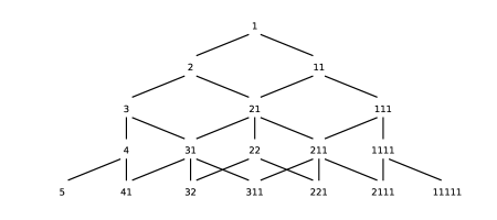
Figure 3: The transition graph for integer partitions

6.2 The cycle view

Above we worked with the order isomorphism aspect of permutations and the associated partial order on $\mathbb{S}$ given by pattern containment. Using cycles instead leads to another partial order on $\mathbb{S}$ where, for $\sigma\in\mathbb{S}_{m}$ and $\tau\in\mathbb{S}_{n}$ with $m\leq n$, the relation $\sigma\leq\tau$ means that in the cycle notation, $\sigma$ arises from $\tau$ by deleting all numbers greater than $m$ (some rearrangement may be necessary to obtain the standard notation). As an example we consider the two sides of (1) again: The order restriction to the set $[4]$ in the one-line notation on the left leads to $3241\in\mathbb{S}_{4}$, which is $(134)(2)$ in standard cycle notation. The cycle restriction to $[4]$ of the permutation on the right hand side is $(1)(432)$ in standard notation, which is $1423$ in one-line notation. In particular, Foata’s correspondence is not consistent with the two notions of restriction.

Nevertheless, the correspondence, together with the construction of $\Pi^{\tiny\rm F}$ on the left hand side, can be used to motivate a Markov chain $\Pi^{\tiny\rm c}=(\Pi^{\tiny\rm c}_{n})_{n\in\mathbb{N}}$ that is adapted to $\mathbb{S}$ and compatible with this order, and has $\Pi^{\tiny\rm c}_{n}\sim\text{\rm unif}(\mathbb{S}_{n})$ for all $n\in\mathbb{N}$. In this construction, known as the Chinese restaurant process, cycles are interpreted as circular tables and customer $n+1$ selects one of the $n$ already seated customers as right neighbor (successor in the cycle notation), or starts a new table, where the $n+1$ possibilities are chosen with the same probability. Note that $\Pi^{\tiny\rm c}$ is projective in the sense that previous values are functions of the present state.

The cycle view is closely related to number partitions: Mapping a permutation to its ordered cycle lengths leads to a function $\Psi:\mathbb{S}\to\mathbb{Y}$ that preserves the grading and the respective partial orders. Let $\Lambda^{\tiny\rm c}=(\Lambda^{\tiny\rm c}_{n})_{n\in\mathbb{N}}$ be defined by $\Lambda^{\tiny\rm c}_{n}:=\Psi(\Pi^{\tiny\rm c}_{n})$ for all $n\in\mathbb{N}$. Then $\Lambda^{\tiny\rm c}$ is again a Markov chain, and it has the cotransitions introduced in Section 6.1 for the family $\mathbb{Y}$. Hence, almost surely as $n\to\infty$, $\Lambda^{\tiny\rm c}_{n}$ converges to an element $(\alpha_{i})_{i\in\mathbb{N}}$ of $\partial\mathbb{Y}_{\text{\tiny\rm c}}$ in the sense that $\lim_{n\to\infty}(\Lambda^{\tiny\rm c}_{n})_{i}/n=\alpha_{i}$ for all $i\in\mathbb{N}$. The distribution of the limit, which is not concentrated at one point of the boundary, can be obtained by stick breaking: Starting with independent and $\text{\rm unif}(0,1)$-distributed random variables $U_{i}$, $i\in\mathbb{N}$, let $(V_{i})_{i\in\mathbb{N}}$ be defined by $V_{1}=U_{1}$ and $V_{n+1}=(1-V_{n})U_{n+1}$ for all $n\in\mathbb{N}$. Putting these in decreasing order provides a random element of $\partial\mathbb{Y}_{\text{\tiny\rm c}}$ that has the same distribution as $\Lambda^{\tiny\rm c}_{\infty}$.

Note that this approach refers to the big cycles. Locally, at the small end, the limit can be obtained from (3): For $i\in\mathbb{N}$ fixed, the counts of cycles of length $k$, $1\leq k\leq i$, are asymptotically independent and Poisson distributed with parameters $1/k$.

The cycle notation displays a permutation as a product of cyclic permutations that act on disjoint parts of the base set. In contrast to the general case such products are commutative. The cycle view is closely connected to the group aspects of permutations, in particular to the representation theory of finite groups. Many probabilists and statisticians became aware of this connection and the resulting ‘non-commutative Fourier analysis’ through Diaconis (1988); more recent and extensive presentations are Ceccherini-Silberstein et al (2008) and Méliot (2017). We briefly summarize some aspects that are relevant to the asymptotics of large permutations. All representations below refer to base field $\mathbb{C}$, ${\text{\rm GL}}(V)$ denotes the general linear (or automorphism) group of the complex vector space $V$, and $U(n)$ is the group of unitary $n\times n$-matrices.

As with compactifications, we begin with an embedding: We regard the elements $g$ of a finite group $G$ as elements of the vector space $\mathbb{C}^{G}$ of functions $f:G\to\mathbb{C}$ via $\sigma\mapsto\delta_{\sigma}$, where $\delta_{\sigma}(\sigma)=1$ and $\delta_{\sigma}(\tau)=0$ if $\tau\not=\sigma$. With the composition of $\sigma,\tau\in G$ written as $\sigma\tau$ we then define convolution on $\mathbb{C}^{G}$ by

$$f\star g(\sigma)=\sum_{\tau\in G}f(\sigma\tau^{-1})\,g(\tau),\quad\sigma\in G.$$

Seen as multiplication, convolution makes $\mathbb{C}^{G}$ an algebra, the group algebra $\mathbb{C}[G]$ associated with $G$. Also, $(\sigma,f)\mapsto\sigma.\,f:=\delta_{\sigma}\star f$ defines an action of $G$ on $V$, and the function $\rho:G\to{\text{\rm GL}}(V)$, $\rho(\sigma)(f):=\sigma.\,f$, is a group homomorphism. With respect to the canonical basis $\{\delta_{\sigma}:\,\sigma\in G\}$ the values $\rho(\sigma)$ are all represented by unitary matrices. Thus, somewhat reminiscent of the fact that every finite group $G$ with $n$ elements is a subgroup of $\mathbb{S}_{n}$, every such $G$ is a subgroup of $U(n)$, both up to group isomorphism. This is known as the (left) regular representation of $G$. More generally, a representation $(\rho,W)$ of $G$ consists of a vector space $W$ and a homomorphism $\rho$ from $G$ to ${\text{\rm GL}}(W)$. For example, representing permutations by their permutation matrices as in (4), we obtain the permutation representation of $G=\mathbb{S}_{n}$.

In a representation $(\rho,W)$ of $G$ a subspace $U$ of $W$ is invariant if $\rho(\sigma)(U)=U$ for all $\sigma\in G$, and the representation is irreducible if only $U=\{0\}$ and $U=W$ are invariant. Necessarily, the range of $\rho$ is then the full group ${\text{\rm GL}}(U)$. It is a crucial fact that the regular representation $(\rho,\mathbb{C}[G])$ can be decomposed into the direct sum $(\bigoplus_{i\in I}\rho_{i},\bigoplus_{i\in I}W_{i})$ of irreducible representations $(\rho_{i},W_{i})$. Let $d_{i}:=\dim W_{i}$. For later use we note that, with $n$ the size of $G$, counting dimensions leads to $\sum_{i\in I}d_{i}^{2}=n$. The character $\chi:G\to\mathbb{C}$ of a representation $\rho$ is given by $\chi(\sigma):=\operatorname{Tr}(\rho(\sigma))$, where $\operatorname{Tr}$ denotes the trace (which does not depend on the basis chosen to represent $\rho(\sigma)$ by a matrix). For the permutation representation $\chi(\sigma)$ is easily seen to be the number of fixed points of $\sigma$.

We recall that general groups can be decomposed into conjugacy classes, which are the equivalence classes obtained when $\sigma,\tau$ are equivalent if $\sigma\pi=\pi\tau$ for some $\pi\in G$. A function $f\in\mathbb{C}[G]$ is a class function or central if it is constant on conjugacy classes. The characters of representations are such class functions, and it turns out that the characters of the irreducible representations constitute a basis for the space (in fact, a convolution algebra) of class functions. Moreover, different irreducible representations lead to different characters. For $G=\mathbb{S}_{n}$ the conjugacy classes correspond to cycle structures and may thus be represented by partitions of $n$, i.e. elements of $\mathbb{Y}_{n}$. Remarkably, the characters of irreducible representations can also be parametrized by such partitions.

This finishes our excursion, and we return to permutation asymptotics. The algebraic point of view mainly refers to characters and thus to partitions, where it leads to a close relative of the Markov chain $\Lambda^{\tiny\rm c}=(\Lambda^{\tiny\rm c}_{n})_{n\in\mathbb{N}}$ discussed above. For this, our main source is the book Kerov (2003); see also the references given there.

It is convenient to augment the permutations of $[n]$ by fixed points so that a bijection of $\mathbb{N}$ is obtained that leaves all $k>n$ invariant. We continue to write $\mathbb{S}_{n}$ for these ‘padded’ versions, and regard them as an increasing sequence of subgroups of the group $\mathbb{S}_{\infty}$ that consists of all finite bijections $\sigma:\mathbb{N}\to\mathbb{N}$, meaning that $\#\{k\in\mathbb{N}:\,\sigma(k)\not=k\}<\infty$. A representation $\rho_{n+1}$ of $\mathbb{S}_{n+1}$ then leads to a representation $\rho_{n}$ of $\mathbb{S}_{n}$ by restriction. This will in general destroy irreducibility, but the character of $\rho_{n}$ is a class function and may thus be written as a linear combination of the irreducible characters on level $n$. It turns out that the non-zero coefficients are all equal to one. Consider now the graph on $\mathbb{Y}$ with edges connecting the character of an irreducible representations on level $n+1$ to the contributing characters of the irreducible representations on level $n$. This is the same graph as the transition graph obtained above for number partitions, see Figure 3, but the edge weights are now all equal to 1. The resulting cotransitions then amount to the rule that, from a current state $\eta\in\mathbb{Y}_{n}$, a state $\lambda\in\mathbb{Y}_{n-1}$ is chosen uniformly at random from its predecessors. The dimension numbers $d_{\lambda}$, $\lambda\in\mathbb{Y}$, turn out to be equal to the number of paths in the diagram that lead from its root to $\lambda$. As a consequence the cotransition associated with an edge $\{\lambda,\eta\}$, $\lambda<\eta$, of the transition graph is given by $d_{\lambda}/d_{\eta}$.

When does a sequence of characters $(\chi_{n})_{n\in\mathbb{N}}$ of irreducible representations or, equivalently, a sequence of partitions $(\lambda(n))_{n\in\mathbb{N}}$, converge in the Doob-Martin topology associated with these cotransitions? Or, in other words, what is the cycle view analog of the pattern frequency topology? The answer requires one more definition: The conjugate (or transpose) of a partition $\lambda=(\lambda_{1},\ldots,\lambda_{k})$ is given by $\lambda^{\star}=(\lambda^{\star}_{1},\ldots,\lambda^{\star}_{j})$ with $j=\lambda_{1}$ and $\lambda^{\star}_{l}=\#\{m\in[k]:\,\lambda_{m}\geq l\}$. Convergence then means that the normalized partition components of $\lambda(n)\in\mathbb{Y}_{n}$ and $\lambda^{\star}(n)$ converge as elements of the unit interval: $\lambda(n)_{i}/n\to\alpha_{i}$, $\lambda^{\star}(n)_{i}/n\to\beta_{i}$ as $n\to\infty$, for all $i\in\mathbb{N}$. The boundary is known as the Thoma simplex,

$$\partial\mathbb{Y}_{\text{\tiny T}}\,=\,\Bigl{\{}(\alpha,\beta)\in[0,1]^{\mathbb{N}}\times[0,1]^{\mathbb{N}}:\,\alpha_{i}\geq\alpha_{i+1},\beta_{i}\geq\beta_{i+1}\text{ for all }i\in\mathbb{N},\ \sum_{i=1}^{\infty}(\alpha_{i}+\beta_{i})\leq 1\Bigr{\}},$$

together with the topology of pointwise convergence. The boundary $\partial\mathbb{Y}_{\text{\tiny\rm c}}$ for the partition chain obtained above in connection with the Chinese restaurant process can be identified with the compact subset of $\partial\mathbb{Y}_{\text{\tiny T}}$ that arises if all $\beta$-values are equal to zero.

A specific combinatorial Markov chain adapted to $\mathbb{Y}$ is given by the Plancherel growth process $\Lambda^{\tiny\rm P}=(\Lambda^{\tiny\rm P}_{n})_{n\in\mathbb{N}}$, with transition probabilities

$$P(\Lambda^{\tiny\rm P}_{n+1}=\eta|\Lambda^{\tiny\rm P}_{n}=\lambda)\,=\,\frac{d_{\eta}}{(n+1)d_{\lambda}},\quad\text{for all }\lambda\in\mathbb{Y}_{n},\,\eta\in\mathbb{Y}_{n+1}\text{ with }\lambda<\eta,$$

and marginal distributions $P(\Lambda^{\tiny\rm P}_{n}=\lambda)=d_{\lambda}^{2}/n!$, $n\in\mathbb{N}$, $\lambda\in\mathbb{Y}_{n}$. It follows from the above dimension counting that the latter are indeed probability mass functions on $\mathbb{Y}_{n}$, and the calculation between Lemma 1 and Theorem 4.1 confirms that $\Lambda^{\tiny\rm P}$ has the cotransitions associated with character restrictions. In contrast to the partition chain $(\Lambda^{\tiny\rm c}_{n})_{n\in\mathbb{N}}$ arising in the cycle length context, the limit distribution for the Plancherel chain $(\Lambda^{\tiny\rm P}_{n})_{n\in\mathbb{N}}$ is concentrated at the one point of the boundary $\partial\mathbb{Y}_{\text{\tiny T}}$ given by $\alpha_{i}=\beta_{i}=0$ for all $i\in\mathbb{N}$. The analysis of this chain leads to some quite spectacular results, such as the arcsine law for the limit shape of Young diagrams, and the solution of Ulam’s problem on the longest increasing subsequences in $\Pi_{n}\sim\text{\rm unif}(\mathbb{S}_{n})$. We refer to Kerov (2003) again, for Ulam’s problem see also Romik (2015).

In connection with trees we had two different graph structures on $\mathbb{B}$. Here the graphs on $\mathbb{Y}$ are the same, but the weights are different. A generalization that includes both the cycle model and the Plancherel process is given in Kerov et al (1998). There, an important aspect is the appearance of classical families of symmetric polynomials in the context of the respective extended Martin kernel.

6.3 Exchangeability

In Section 4 we worked with a general Markov chain $X=(X_{n})_{n\in\mathbb{N}}$ that is adapted to a graded state space $S=\bigsqcup_{n\in\mathbb{N}}S_{n}$ and we used the cotransitions of $X$ to obtain a compactification $\bar{S}=S\sqcup\partial S$ of the state space, together with a limit variable $X_{\infty}$ for the $X_{n}$’s as $n\to\infty$. Each boundary value $\alpha\in\partial S$ induces a probability measure $P^{\alpha}$, which is the model for $X$ conditioned on $X_{\infty}=\alpha$. Further, an arbitrary distribution $\mu$ on the Borel subsets of $\partial S$ may be used to construct a Markov chain that has the same cotransitions as $X$ and limit distribution $\mathcal{L}(X_{\infty})=\int P^{\alpha}\,\mu(d\alpha)$, the $\mu$-mixture of the $P^{\alpha}$’s. We note that this is the time reversal version of the familiar ‘forward’ situation where the distribution of a Markov chain is specified by the distribution of the first variable and the (forward) transition probabilities. Here, however, the distribution of $X_{\infty}$ is usually defined on a non-discrete space, and there is of course no step from $\infty$ to ‘$\infty-1$’.

The above shows some similarities to the archetypical exchangeability result, de Finetti’s theorem: We start with a sequence $X=(X_{n})_{n\in\mathbb{N}}$ of real random variables that is exchangeable in the sense that the distribution $\mathcal{L}(X)$ of $X$ is invariant under all $\sigma\in\mathbb{S}_{\infty}$, the set of finite permutations of $\mathbb{N}$ introduced in Section 6.2. We then obtain a limit $M_{\infty}$ for the empirical distributions $M_{n}:=\frac{1}{n}\sum_{i=1}^{n}\delta_{X_{i}}$ and it holds that $\mathcal{L}(X|M_{\infty}=\mu)=\mathcal{L}(\tilde{X})$ where $\tilde{X}=(\tilde{X}_{i})_{i\in\mathbb{N}}$ with $\tilde{X}_{i}$, $i\in\mathbb{N}$, independent random variables with distribution $\mu$. This area has developed into a major branch of modern probability, dealing with structural results for distribution families with certain invariance properties. Kallenberg (2005) is a standard reference, but see also Aldous (1985) and Austin (2008). An excellent introduction is also given in the first part of the lecture notes Austin (2013).

Exchangeability may provide an approach to the asymptotics of random discrete structures; see e.g. Section 11.3.3 in Lovasz (2012) for graphs and Evans et al (2017) for Rémy trees. (In the other direction, a proof for the classical de Finetti theorem can be given using Markov chain boundary theory; see Gerstenberg et al (2016).) In their treatment of random permutations and permutons Hoppen et al (2013) emphasize the connection to random graphs and graphons. Our aim here is to extend this to the exchangeability aspect.

In the subgraph frequency topology for sequences of (random) graphs the limits are described by a (possibly random) graphon, a measurable and symmetric function $W:[0,1]\times[0,1]\to[0,1]$. Given $W$, we use a sequence $U=(U_{i})_{i\in\mathbb{N}}$ of independent uniforms to construct a random binary $\mathbb{N}\times\mathbb{N}$-matrix $Z$ by choosing $Z_{ij}=Z_{ij}=1$ with probability $W(U_{i},U_{j})$, $1\leq i<j<\infty$, independently for different pairs, and $Z_{ii}=0$ for all $i\in\mathbb{N}$. This matrix is jointly exchangeable in the sense that, for all $\sigma\in\mathbb{S}_{\infty}$, $Z^{\sigma}:=(Z_{\sigma(i),\sigma(j)})_{i,j\in\mathbb{N}}$ has the same distribution as $Z$. The upper $n\times n$-corner of $Z$ is the incidence matrix of a random graph $G_{n}$. As $n\to\infty$, these converge in the subgraph frequency topology, and the limit is represented by $W$. The graphon may be regarded as an analogue of the measure $M_{\infty}$ in the classical case of exchangeable sequences, and the second step as an analogue of sampling from $M_{\infty}$.

Is there a similar representation for random permutations, specifically for the copula-based models in part (c) of Theorem 3.1? We need an infinite matrix that represents the complete sequence, with the upper left $n\times n$-corner for the result of the first $n$ steps. Starting with independent random vectors $(X_{i},Y_{i})$, $i\in\mathbb{N}$, with distribution function $C$, we define an infinite random binary array $Z=(Z_{ij})_{i,j\in\mathbb{N}}$ by

$$Z_{ij}=\begin{cases}1,&\text{if }i<j\text{ and }Y_{i}<Y_{j},\\ 1,&\text{if }i>j\text{ and }X_{i}<X_{j},\\ 0,&\text{else.}\end{cases}$$

For example, if the cities in our data set arrive in order of decreasing population size (Berlin, Hamburg, Munich, Cologne $\ldots$) then the upper left $4\times 4$-corner of $Z$ is

$$(Z_{ij})_{i,j=1}^{4}\;=\;\begin{pmatrix}0&1&0&0\\ 0&0&0&0\\ 0&1&0&1\\ 0&0&0&0\\ \end{pmatrix}.$$

Within this group, there is one city with more citizens than Munich that is further to the east, and none of them is further to the south. The permutation $\Pi_{n}$ can be obtained from $(Z_{ij})_{1\leq i,j\leq n}$ as follows: With

$$\#\bigl{\{}1\leq i\leq n:\,X_{j}\leq X_{i}\bigr{\}}\;=\ \sum_{i=1}^{j-1}Z_{ij}\,+\,(n-j-1)\;-\sum_{i=j+1}^{n}Z_{ij},\quad 1\leq j\leq n,$$

we get the absolute ranks of the variables $X_{i}$, $1\leq i\leq n$, within $\{X_{1},\ldots,X_{n}\}$, and a similar formula holds for the $Y$-components. Then $\Pi_{n}$ can be determined from the two rank vectors as in (6). Equivalently, we may work with an array $\tilde{Z}$ indexed by subsets $\{i,j\}$ of $\mathbb{N}$ of size two, $i<j$, by using the values $0,1,2,3$ for indicating the relative position of $(X_{j},Y_{j})$ with respect to $(X_{i},Y_{i})$ through the four quadrants North-East (NE), SE, SW, and NW.

If $\sigma:\mathbb{N}\to\mathbb{N}$ is strictly increasing, then the matrix $Z^{\sigma}$ with entries $Z_{\sigma(i),\sigma(j)}$ depends on $(X_{\sigma(i)},Y_{\sigma(i)})$, $i\in\mathbb{N}$, in the same (deterministic) way as $Z$ depends on $(X_{i},Y_{i})$, $i\in\mathbb{N}$. As the subsequence $(X^{\sigma},Y^{\sigma})$ is equal in distribution to the original sequence $(X,Y)$, the arrays $Z^{\sigma}$ and $Z$ are then equal in distribution, which shows that $Z$ is contractable. An analogous statement holds for the corresponding array $\tilde{Z}$ indexed by size two subsets of $\mathbb{N}$. It follows from the general Aldous-Hoover-Kallenberg representation theorem that a contractable array can be extended to an exchangeable array; see Corollary 7.16 in Kallenberg (2005).

In order to construct a suitable graphon analogue $W$ we note that the copula $C$ represents a distribution on the unit square and thus may be written as a composition of the distribution function of the first variable and the conditional distribution function $G(x,\cdot)$ of the second variable, given the value $x$ for the first. Let

$$W(x,y):=\inf\{z\in[0,1]:\,G(x,z)\geq y\},\quad 0\leq y\leq 1,$$

be the corresponding quantile function. Further, let $(U_{i})_{i\in\mathbb{N}}$ and $(V_{i})_{i\in\mathbb{N}}$ be two independent sequences of independent $\text{\rm unif}(0,1)$-distributed random variables. By construction, $(X_{i},Y_{i})=_{\text{\rm\tiny distr}}(U_{i},W(U_{i},V_{i}))$ for all $i\in\mathbb{N}$, and by independence, this even holds for the two sequences. Thus the random binary matrix $\tilde{Z}=(\tilde{Z}_{ij})_{i,j\in\mathbb{N}}$ given by

$$\tilde{Z}_{ij}=\begin{cases}1,&\text{if }i<j\text{ and }W(U_{i},V_{i})<W(U_{j},V_{j}),\\ 1,&\text{if }i>j\text{ and }U_{i}<U_{j},\\ 0,&\text{else,}\end{cases}$$

has the same distribution as $Z$. Of course, the conditional construction could have been done in the other direction. It is indeed quite common in these constructions that uniqueness of the representation only holds up to some equivalence, which may be difficult to describe.

It is of interest to know whether an exchangeable array is ergodic. For exchangeable sequences $(X_{i})_{i\in\mathbb{N}}$ this means that $M_{\infty}\equiv\mu$ for some fixed distribution $\mu$, so that the $X_{i}$’s are independent. In the permuton situation such extreme points correspond to a fixed copula, and this is always the case for the models in Theorem 3.1 (c). One of the interesting aspects of the results in Bassino et al (2018) is the fact that, for separable permutations, the limit object is not degenerate.

Above we have used random matrices in order to point out the similarity to random graphs and graphons. A more abstract and more general approach has been developed in Gerstenberg (2018), where cartesian products of total orders on $\mathbb{N}$ are considered and ergodicity is discussed in some detail.

6.4 Some connections to statistical concepts

Markov chain boundaries and exchangeable sequences both lead to parametrized families of probability distributions, where the parameter is the value of $X_{\infty}$ in the first case and the value of $M_{\infty}$ in the second. A relationship between the Martin boundary of Markov chains and parametric families has been pointed out early by Abrahamse (1970), together with a connection to exponential families which, roughly, appear as $h$-transforms in certain situations. Section 18 in Aldous (1985) deals with sufficiency and mixtures in the context of exchangeable random structures. In the framework of combinatorial Markov chains $(X_{n})_{n\in\mathbb{N}}$ discussed above, where we regard the value of $X_{\infty}$ in the Doob-Martin compactification as a parameter $\theta$ and the values of the first $n$ variables $X_{1},\ldots,X_{n}$ as data, it is clear that $X_{n}$ is a sufficient statistic for $\theta$ as the conditional law of the data given $X_{n}$ can be reconstructed from the cotransitions, and these do not depend on $\theta$. Lauritzen (1974) used this as a basis for his concept of total sufficiency; the paper also discusses a variety of related aspects. Lauritzen (1988) emphasizes the role of the Martin boundary as a basic concept.

Further, both the set of distributions on the boundary and the set of directing measures are convex, and ‘pure parameters’ or ‘extreme models’ correspond to the ergodic case, which are extremal elements of the respective convex set. This aspect has appeared repeatedly in the above examples. Dynkin (1978) introduced H-sufficiency, dealing with the question of whether the convex set is a simplex (in a barycentric sense). The latter points to a connection with geometry; see Baringhaus and Grübel (2021) for a recent contribution.

Two final comments may be in order, both are somewhat loose. First, as seen above, large random discrete structures can be investigated through the Doob-Martin boundary of Markov chains, or through the representation of exchangeable distributions. The first is based on the topological approach of constructing a limit for a sequence of growing objects, the second is based on the construction of an ‘asymptotic template’ from which the sequence can be obtained by sampling, and is of a more measure-theoretical nature. (Poisson boundaries, which we did not discuss, may be seen as a measure-theoretical variant of the former.) A similar distinction appears in connection with convex sets, with Choquet’s theorem for topological vector spaces, and the barycenter approach motivated by potential theory. As a second comment, we note that permutations appear naturally in classical nonparametric statistics, where ranks are a basic tool, but that other combinatorial families may similarly be analyzed with a view towards statistical applications. Often the results on the discrete structures themselves can serve as a basis for obtaining asymptotics for a variety of specific aspects, in some resemblance to using functional limit theorems to obtain distributional limit theorems for a variety of specific statistics.

Conflict of interest

The author declares that he has no conflict of interest.

References

- Abrahamse (1970) Abrahamse, A.F. (1970) A comparison between the Martin boundary theory and the theory of likelihood ratios. Ann. Math. Statistics 41: 1064–1067.
- Aldous (1985) Aldous, D.J. (1985) Exchangeability and related topics. Lecture Notes in Math. 1117: 1–-198. Springer, Berlin.
- Arratia et al (2003) Arratia, R., Barbour, A.D., Tavaré, S. (2003) Logarithmic combinatorial structures: a probabilistic approach. European Mathematical Society, Zürich.
- Austin (2008) Austin, T. (2008) On exchangeable random variables and the statistics of large graphs and hypergraphs. Probability Surveys 5: 80–145.
- Austin (2013) Austin, T. (2013) Exchangeable random arrays. Lecture Notes, www.math.ucla.edu/tim/notes.html.
- Baringhaus and Grübel (2021) Baringhaus, L., Grübel, R. (2021) Discrete mixture representations of parametric distribution families: Geometry and statistics. Electronic Journal of Statistics 15: 37-–70
- Baringhaus and Grübel (2022) Baringhaus, L., Grübel, R. (2022) Random permutations generated by delay models and estimation of delay distributions. In preparation.
- Bassino et al (2018) Bassino, F., Bouvel, M., Féray, V., Gerin, L., Pierrot, A. (2018) The Brownian limit of separable permutations. Ann. Probab. 46: 2134–2189.
- Bona (2004) Bona, M. (2004) Combinatorics of Permutations. Chapman and Hall, Boca Raton.
- Ceccherini-Silberstein et al (2008) Ceccherini-Silberstein, T., Scarabotti, F., Tolli, F. (2008) Harmonic analysis on finite groups. Cambridge University Press, Cambridge.
- Cox and Smith (1961) Cox, D.R., Smith, W.L. (1961) Queues. Chapman and Hall, London.
- Crudele et al (2023) Crudele, G., Dukes, P. and Noel, J.A. (2023) Six permutation patterns force quasirandomness. Available at: arXiv:2303.04776.
- Diaconis (1988) Diaconis, P. (1988). Group representations in probability and statistics. Institute of Mathematical Statistics Lecture Notes—Monograph Series 11. Hayward, CA.
- Diaconis and Janson (1988) Diaconis, P., Janson, S. (2008) Graph limits and exchangeable random graphs. Rend. Mat. Appl. 28: 33–61.
- Doob (1959) Doob, J.L. (1959) Discrete potential theory and boundaries. J. Math. Mech. 8: 433–458.
- Dynkin (1978) Dynkin, E.B. (1978). Sufficient statistics and extreme points. Ann. Probab. 6: 705–730.
- Evans al (2012) Evans, S.N., Grübel, R., Wakolbinger, A. (2012) Trickle-down processes and their boundaries. Electron. J. Probab. 17: 58pp.
- Evans et al (2017) Evans, S.N., Grübel, R., Wakolbinger, A. (2017) Doob–Martin boundary of Rémy’s tree growth chain. Ann. Probab. 45: 225-277.
- Feller (1968) Feller, W. (1968) An Introduction to Probability Theory and Its Applications. Vol. I, 3rd ed.. Wiley, New York.
- Gerstenberg (2018) Gerstenberg, J. (2018) Austauschbarkeit in Diskreten Strukturen: Simplizes und Filtrationen. Dissertation. Leibniz Universität Hannover.
- Gerstenberg et al (2016) Gerstenberg, J., Grübel, R., Hagemann, K. (2016) A boundary theory approach to de Finetti’s theorem. Available at: https://arxiv.org/abs/1610.02561.
- Grübel (2013) Grübel, R. (2013) Kombinatorische Markov-Ketten. Math. Semesterber. 60: 185–-215
- Grübel (2015) Grübel, R. (2015) Persisting randomness in randomly growing discrete structures: graphs and search trees. Discrete Mathematics & Theoretical Computer Science 18: 23pp.
- Hagemann (2016) Hagemann, K. (2016) Doob-Martin-Theorie diskreter Markov-Ketten: Struktur und Anwendungen. PhD thesis, Leibniz Universität Hannover.
- Hoppen et al (2013) Hoppen, C., Kohayakawa, Y., Moreira, C.G., Ráth, B., Sampaio, R.M. (2013) Limits of permutation sequences. J. Comb. Theory, Ser. B 103: 93–113.
- Janson (2020) Janson, S. (2020) Patterns in random permutations avoiding some sets of multiple patterns. Algorithmica 82, 616–641.
- Kallenberg (2005) Kallenberg, O. (2005) Probabilistic symmetries and invariance principles. Springer, New York.
- Kelley (1955) Kelley, J.L. (1955) General topology. Van Nostrand Company, Toronto-New York-London.
- Kerov et al (1998) Kerov, S.V., Okounkov, A., Olshanski, G. (1998) The boundary of the Young graph with Jack edge multiplicities. Int. Mathematics Research Notices: 173–199.
- Kerov (2003) Kerov, S. V. (2003) Asymptotic representation theory of the symmetric group and its applications in analysis. Translations of Mathematical Monographs 219. American Mathematical Society, Providence, RI.
- Král and Pikhurko (2013) Král, D., Pikhurko, O. (2013) Quasirandom permutations are characterized by 4-point densities. Geom. Funct. Anal. Vol. 23: 570–-579.
- Lauritzen (1974) Lauritzen, S. L. (1974) Sufficiency, prediction and extreme models. Scand. J. Statist. 1: 128–134.
- Lauritzen (1988) Lauritzen, S.L. (1988) Extremal families and systems of sufficient statistics. Lecture Notes in Statistics 49. Springer, Berlin.
- Lovasz (2012) Lovász, L. (2012) Large networks and graph limits. American Mathematical Society Colloquium Publications 60. Amer. Math. Soc., Providence, RI.
- Méliot (2017) Méliot, P.-L. (2017) Representation theory of symmetric groups. CRC Press, Boca Raton.
- Nelson (2006) Nelson, R.B. (2006) An introduction to copulas, 2nd ed. Springer, New York.
- Romik (2015) Romik, D. (2015) The surprising mathematics of longest increasing subsequences. Institute of Mathematical Statistics Textbooks 4, Cambridge University Press, New York.
- Shi et al (2022) Shi, H., Drton, M. and Han, F. (2022) On the power of Chatterjee’s rank correlation. Biometrika 109, 317–333.
- van der Vaart (1998) van der Vaart, A.W. (1998) Asymptotic Statistics. Cambridge University Press, Cambridge.
- Woess (2009) Woess, W. (2009) Denumerable Markov chains. European Mathematical Society, Zürich.
- Yanagimoto (1970) Yanagimoto, T. (1970) On measures of association and a related problem. Ann. Inst. Stat. Math. 22, 57–63.