Quasi-stable Coloring for Graph Compression

Abstract.

We propose quasi-stable coloring, an approximate version of stable coloring. Stable coloring, also called color refinement, is a well-studied technique in graph theory for classifying vertices, which can be used to build compact, lossless representations of graphs. However, its usefulness is limited due to its reliance on strict symmetries. Real data compresses very poorly using color refinement. We propose the first, to our knowledge, approximate color refinement scheme, which we call quasi-stable coloring. By using approximation, we alleviate the need for strict symmetry, and allow for a tradeoff between the degree of compression and the accuracy of the representation. We study three applications: Linear Programming, Max-Flow, and Betweenness Centrality, and provide theoretical evidence in each case that a quasi-stable coloring can lead to good approximations on the reduced graph. Next, we consider how to compute a maximal quasi-stable coloring: we prove that, in general, this problem is NP-hard, and propose a simple, yet effective algorithm based on heuristics. Finally, we evaluate experimentally the quasi-stable coloring technique on several real graphs and applications, comparing with prior approximation techniques.

Artifact Availability:
The source code, data, and/or other artifacts have been made available at https://github.com/mkyl/QuasiStableColors.jl.

1. Introduction

A well known technique for finding structure in large graphs is the color refinement, or 1-dimensional Weisfeiler-Leman method. It consists of assigning the nodes in the graph some initial color, for example based on their labels. Then one repeatedly refines the coloring, by assigning distinct colors to two nodes whenever those nodes have a different number of neighbors of the same color; when no more refinement is possible, then this is called a stable coloring. We show a simple illustration in Fig. 1 (a): for example nodes 5 and 11 have the same dark purple color, because both have one purple, one lavender, and one dark purple neighbor, while node 7 has a different color because it additionally has an olive neighbor. The stable coloring can be computed efficiently, in almost linear time (Paige and Tarjan, 1987), can be generalized to labeled graphs, weighted graphs, directed or undirected graphs, and multigraphs, and is used by graph isomorphism algorithms (Grohe and Schweitzer, 2020), in graph kernels (Shervashidze and Borgwardt, 2009), and more recently has been used to explain and enhance the power of Graph Neural Networks (Xu et al., 2019; Morris et al., 2019; Grohe, 2020; Morris et al., 2021a). We review stable coloring in Sec. 2. Excellent surveys of color refinement and its recent applications to machine learning can be found in (Morris et al., 2021b; Grohe, 2020, 2021).

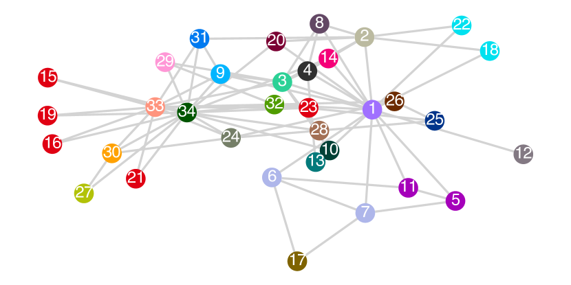
(a) Stable coloring

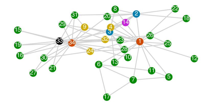
(b) Quasi-stable coloring, $q=3$

Figure 1. Coloring Zachary’s karate club graph (Zachary, 1977) where $|V|=34$, $|E|=78$. While the stable coloring requires $27$ colors, for a quasi-stable color $6$ colors suffice when $q=3$. Note in 1(b) the club leaders $\mathinner{\left\{1,34\right\}}$ are put into their own color.

In this paper we apply stable coloring as a compression technique for large graphs. A stable coloring naturally defines a reduced graph, whose nodes are the classes of colors of the original graph. The new graph preserves many important properties of the original graph, which makes it a good candidate for compression. For example, an elegant theoretical result states that the reduced graph satisfies precisely the same properties expressible in the $C^{2}$ logic as the original graph (Grohe and for Symbolic Logic, 2017). Motivated by the fact that the reduced graph preserves key properties of the original graph, Grohe et al. (Grohe et al., 2014; Grohe et al., 2021) propose using color refinement as a dimensionality reduction technique, and show two applications: to Linear Programming and to graph kernels.

However, we notice that stable coloring is not effective for dimensionality reduction because, in practice, the “reduced” graph is only slightly smaller than the original graph. For example, the graph in Fig 1 (a) has 34 nodes, but 27 colors, which means that the reduced graph has 80% of the number of nodes of the original. We show in Sec. 6 that, for typical large graphs, the size of the reduced graph is between 70% - 80% that of the original graph. Moreover, even when a graph happens to have a small reduced graph, any tiny update, e.g. adding or deleting an edge, will immediately lead to a huge increase of the reduced graph. We illustrate this phenomenon briefly in Fig. 2: we started with an artificially regular graph, which compressed well from 1000 nodes to only 100 colors, but the compression degrades very rapidly when we add only a few edges.

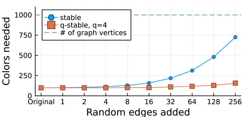
Figure 2. Comparing the robustness of stable and q-stable coloring. A synthetic graph with $|V|=1~{}000,|E|=21~{}600$ is generated with a size $100$ stable and q-stable coloring. As a small fraction of edges (no more than $1.5\%$) are added, the brittleness of stable coloring causes compression to degenerate—quasi-stable colors are immune to this.

In this paper we propose a generalization of stable coloring to quasi-stable coloring, with a goal of reducing the size of the compressed graph while still allowing applications to be processed approximatively. Our definition of $q$-stable coloring, given in Sec. 3, allows two nodes to be in the same color if they have a number of neighbors to any another color that differs by at most $q$, where $q\geq 0$ is a parameter. This has dual effect. First, it can dramatically reduce the size of the compressed graph, since more nodes can now be assigned the same color. For example, the quasi-stable coloring in Fig. 1 (b) allows nodes 5 and 7 to have the same color, even though their number of green neighbors differs by 1; the new compressed graph has only 6 nodes. Second, this makes the technique less sensitive to data updates, because it can tolerate nodes with a slightly different number of neighbors. We can see in Fig. 2 that the number of quasi-stable colors increases only marginally with the addition of random edges. By varying the parameter $q$, the quasi-stable colors offer a tradeoff between the compression ratio and the degree to which the reduced graph preserves the properties of the original graph.

We start by investigating in Sec. 4 whether the result of an application over the reduced graph is a good approximation of the result on the original graph. We consider three applications: linear programming, max flow, and betweenness centrality. In all three cases we provide a theoretical justification for why the result on the reduced graph should be close to the true value. First, for linear programs, we prove that the optimal value of the reduced program converges to the optimal value of the original program when $q\rightarrow 0$. This generalizes the result in (Grohe et al., 2014), which proved that, when the coloring is stable ($q=0$) then the LP has the same optimal value on reduced program and the original program. Next, for the max flow problem we prove that, while pathological cases exist where a “good” quasi-stable coloring has a totally different max-flow than the original graph, under reasonable assumptions the two are close and, in particular, when the coloring is stable ($q=0$) then they are equal. Third, we examine betweenness centrality, and show that, even a stable coloring can, in pathological cases, lead to different centrality scores, but we prove that the 2-WL method (a refinement of 1-WL) always preserves the centrality score.

Next, in Section 5 we study the algorithmic problem of efficiently computing a quasi-stable coloring for a graph. While the stable coloring can be computed in almost linear time, we prove, rather surprisingly, that finding an optimal quasi-stable coloring is NP-hard. The main difference is that there is always a maximum, “best”, stable coloring, but none exist in general for quasi-stable coloring. Based on this observation, we propose a heuristic-based algorithm for computing a quasi-stable coloring, whose decisions are informed by our theoretical analysis in Sec. 4.

Finally, we conduct an empirical evaluation of quasi-stable coloring in Section 6. Testing on twenty datasets from a variety of domains, we find q-stable colorings favorably trade-off accuracy for speed. For example, on the qap15 linear program, an exact solution takes 22 minutes to compute while the q-stable approximation reduces the problem size by $100\times$, solving it end-to-end within 17 seconds while introducing only a 5% error. We observe similar trends for max-flow and centrality applications. Next, we study the characteristics of the compressed graphs, finding that they avoid the pitfalls of stable colorings. We conclude by characterizing our algorithm, analyzing its runtime, its ability to progressively improve the approximations and testing its robustness to noise.

In summary, we make the following contributions in this paper:

• We propose a relaxation of stable coloring, called quasi-stable coloring; Sec. 3.

• We provide theoretical evidence that the reduced graph defined by a quasi-stable coloring can be useful in three classes of applications; Sec. 4.

• We prove that an optimal quasi-stable coloring is NP-hard to compute, and propose an efficient, heuristic-based algorithm; Sec. 5.

• We conduct an experimental evaluation on several real graphs and applications; Sec. 6.

2. Background on Color Refinement

Fix an undirected graph $G=(V,E)$. We denote by $N(x)$ the set of neighbors of a node $x\in V$. A coloring of $G$ is a partition of $V$ into $k$ disjoint sets, $V=P_{1}\cup\cdots\cup P_{k}$. We say that a node $x\in P_{i}$ has color $i$, or that it has color $P_{i}$. We denote the coloring by $\bm{P}=\mathinner{\left\{P_{1},\ldots,P_{k}\right\}}$. A stable coloring is a coloring with the property that, for any two colors, all nodes in the first color have the same number of neighbors in the second color. Formally:

$$\forall i,j,\forall x,y\in P_{i}\mathrel{\mathop{\ordinarycolon}}\ \ |N(x)\cap P_{j}|=|N(y)\cap P_{j}|$$

Given two colorings $\bm{P},\bm{P}^{\prime}$ we say that the first is a refinement of the second, and denote this by $\bm{P}\subseteq\bm{P}^{\prime}$, if for every color $P_{i}\in\bm{P}$, there exists a color $P_{j}^{\prime}\in\bm{P}^{\prime}$ such that $P_{i}\subseteq P_{j}^{\prime}$. Any two colorings $\bm{P},\bm{P}^{\prime}$ have a greatest lower bound, $\bm{P}\wedge\bm{P}^{\prime}$, and a least upper bound, $\bm{P}\vee\bm{P}^{\prime}$. The greatest lower bound is easily constructed, by considering the partition $\{{P_{i}\cap P_{j}^{\prime}}\mid{P_{i}\in\bm{P},P_{j}^{\prime}\in\bm{P}^{\prime}}\}$; for a construction of $\bm{P}\vee\bm{P}^{\prime}$, we refer the reader to (Stanley, 2012).

The smallest coloring, where each node $x$ is in a separate color, denoted $\bm{P}_{\bot}$, is trivially a stable coloring. Somewhat less obvious is the fact that, if both $\bm{P}$ and $\bm{P}^{\prime}$ are stable colorings, then their least upper bound $\bm{P}\vee\bm{P}^{\prime}$ is also a stable coloring (see also Th. 1 below). This implies that every graph has a unique, maximum stable coloring, often called the stable coloring of $G$, namely $\bm{P}_{1}\vee\bm{P}_{2}\vee\cdots$, where $\bm{P}_{1},\bm{P}_{2},\ldots$ are all stable colorings of the graph. The stable coloring can be computed quite efficiently using the color refinement method, sometimes also called the 1-dimensional Weifeiler-Leman method (1WL). Start by coloring all nodes with the same color, then repeatedly choose two colors $P_{i},P_{j}$ and refine the set $P_{i}$ by partitioning its nodes based on their number of neighbors in $P_{j}$; the stable coloring is obtained when no more refinement is possible. There exist improved algorithms that compute the stable coloring in time $O(n+m\log n)$, where $n,m$ are the number of nodes and edges respectively (Morris et al., 2021b). The reduced graph, $\hat{G}$, has one node $i$ for each color $P_{i}$, and an edge from $i$ to $j$ if some node $x\in P_{i}$ has a neighbor $y\in P_{j}$ (in which case every node $x\in P_{j}$ has a neighbor $y\in P_{j}$).

Color refinement can be generalized to directed graphs, to labeled graphs, to multi-graphs, and to weighted graphs. We refer the reader to (Morris et al., 2021b) for an extensive survey of the theoretical properties of the color refinement method. In this paper we will consider directed, weighted graphs, but defer their discussion to Sec. 3.

Most applications of stable coloring work best on graphs that have many colors, i.e. where there are many, small sets $P_{i}$. For example, in order to check for an isomorphism between two graphs $G,G^{\prime}$, one first computes the stable coloring of the disjoint union of $G$ and $G^{\prime}$, then restricts the isomorphisms candidates to functions that preserve the color of the nodes. The best case is when the stable coloring is $\bm{P}_{\bot}$, because then the only possible isomorphism is the function that maps $x\in G$ to the similarly colored $y\in G^{\prime}$. In general, applications of the 1WL method work best when there are many colors.

In this paper we use coloring for dimensionality reduction and approximate query processing. Instead of solving the problem on the original, large graph $G$, we solve it on the reduced graph $\hat{G}$. This technique works best when there are few colors, because then the reduced graph is small. Real graphs tend to have many colors; we found (see Sec. 6) that the number of colors is typically around 70% of the number of nodes. This observation has a theoretical justification: if $G$ is a random graph, then with high probability its stable coloring is $\bm{P}_{\bot}$ (Morris et al., 2021b, Sec.3.3). This motivated us to introduce a new notion, quasi-stable coloring, which relaxes the stability condition, in order to allow us to construct fewer, larger colors.

3. Quasi-stable Coloring

We have seen that the stable coloring of a graph has many elegant properties, but offers poor compression in practice. In this section we introduce a relaxed notion, which preserves some of the desired properties while improving the compression.

A weighted directed graph $G=(X,E,w)$ is a directed graph with a function $w$ mapping edges to real numbers. We will assume that the edge $(x,y)$ exists iff $w(x,y)\neq 0$, and therefore we often omit $E$ and simply write the directed graph as $G=(X,w)$. Conversely, given a standard graph $G=(X,E)$, we assume a default weight function $w(x,y)=1$ when $(x,y)\in E$ and $w(x,y)=0$ otherwise. A bipartite graph is a graph where the nodes consist of two sets $X,Y$ and all edges go from some node in $X$ to some node in $Y$. We denote a bipartite graph by $(X,Y,E)$ or $(X,Y,w)$ if it is weighted.

Given a weighted graph $(X,w)$ and two subsets of nodes $U,V$, we denote by $w(U,V)$ the total weight from $U$ to $V$:

(1) $$w(U,V)\stackrel{{\scriptstyle\text{def}}}{{=}} \sum_{x\in U,y\in V}w(x,y)$$

Fix a reflexive and symmetric relation $\sim$ on $\mathbb{R}$.

Definition 1.

(1) Let $G=(X,Y,w)$ be a weighted, bipartite graph (i.e. $w\mathrel{\mathop{\ordinarycolon}}X\times Y\rightarrow\mathbb{R}$). We say that $G$ is $\sim$regular if the following two conditions hold:

$$\forall x_{1},x_{2}\in X\mathrel{\mathop{\ordinarycolon}}\ w(x_{1},Y)\sim w(x_{2},Y)$$

$$\forall y_{1},y_{2}\in Y\mathrel{\mathop{\ordinarycolon}}\ w(X,y_{1})\sim w(X,y_{2})$$

(2) Let $G=(X,w)$ be any weighted, directed graph, and $\bm{P}=\mathinner{\left\{P_{1},\ldots,P_{k}\right\}}$ be a partition of its nodes. We say that $\bm{P}$ is $\sim$quasi-stable, or quasi-stable w.r.t. $\sim$, if, for any two colors $P_{i},P_{j}$ (including $i=j$), the bipartite graph $(P_{i},P_{j},w)$ is $\sim$regular.

Thus, a quasi-stable coloring partitions the nodes in such a way that for any two colors $P_{i},P_{j}$, any two nodes in $P_{i}$ have similar (according to $\sim$) outgoing weights to $P_{j}$, and any two nodes in $P_{j}$ have similar incoming weights from $P_{i}$.

3.1. Examples

We illustrate with several examples.

Biregular Graphs, and Stable Coloring Recall that a bipartite graph $(X,Y,E)$ is $(a,b)$-biregular, or simply biregular when $a,b$ are clear from the context, if every node $x\in X$ has outdegree $a$ and every node in $y\in Y$ has indegree $b$. Let $\sim$ be the equality relation on $\mathbb{R}$: $u\sim v$ iff $u=v$. Then $(X,Y,E)$ is $=$regular iff it is biregular. Furthermore, if $G$ is a directed graph, then a coloring $\bm{P}$ is $=$quasi-stable iff it is stable.

$q$-Stable Coloring The main type of quasi-stable coloring that we use in this paper is called $q$-stable. Fix some number $q\geq 0$, and define the following similarity relation on $\mathbb{R}$: $u\sim_{q}v$ if $|u-v|\leq q$. Notice that $\sim_{q}$ is reflexive and symmetric, but not transitive. In a $\sim_{q}$regular bipartite graph any two nodes in $X$ have outgoing weights that differ by at most $q$, and similarly for the incoming weights of the nodes in $Y$. To reduce clutter, we will call a $\sim_{q}$quasi-stable coloring a $q$-stable coloring, or simply a $q$-coloring. The standard stable coloring is the special case when $q=0$.

$\varepsilon$-Relative Coloring While $q$-stable coloring imposes a bound on the absolute error, we briefly discuss an alternative: imposing a bound on the relative error. Fix some number $\varepsilon\geq 0$, and define $u\sim^{\varepsilon}v$ as $u\cdot e^{-\varepsilon}\leq v\leq u\cdot e^{\varepsilon}$. This relation is reflexive and symmetric, but not transitive. We call a $\sim^{\varepsilon}$quasi-stable coloring simply a $\varepsilon$-relative coloring. Notice that isolated nodes (i.e. without incoming or outgoing edges) are in a separate color. This is because zero is similar only to itself: $u\sim^{\varepsilon}0$ implies $u=0$. More generally, for any two colors, either every node in the first color is connected to some node in the second, or none is, and similarly with the role of the two colors reversed.

Bisimulation Relation As a last example, define $u\equiv v$ as $u=v=0$ or $u\neq 0,v\neq 0$. In other words, $\equiv$ checks if both $u,v$ are zero, or none is zero. This is an equivalence relation. Then, a $\equiv$quasi-stable coloring is a bisimulation relation on that graph (Grohe and for Symbolic Logic, 2017).

3.2. The Reduced Graph

Let $G=(X,w)$ be a directed, weighted graph and let $\bm{P}=\mathinner{\left\{P_{1},\ldots,P_{k}\right\}}$ be any coloring, not necessarily quasi-stable. The reduced graph, is defined as $\hat{G}\stackrel{{\scriptstyle\text{def}}}{{=}}(\hat{X},\hat{w})$, where the nodes $\hat{X}\stackrel{{\scriptstyle\text{def}}}{{=}}\mathinner{\left\{1,2,\ldots,k\right\}}$ correspond to the colors. We will consider different choices for the weight function; one example is that we can set it to be the sum of all weights between two colors, i.e. $\hat{w}(i,j)\stackrel{{\scriptstyle\text{def}}}{{=}}\sum_{x\in P_{i};y\in P_{j}}w(x,y)$, but we will consider other options too. Our goal in this paper is to use the reduced graph to compute approximate answers to problems that are expensive to compute on the original, large graph.

4. Applications

Stable coloring preserves many nice properties of the graph. Will a $q$-quasi stable coloring preserve such properties to some degree? We explore this question here, and provide theoretical evidence that quasi stable colorings provide some useful approximations for three problems: linear optimization, maximum flow, and betweenness centrality. In Section 6 we validate experimentally these findings.

4.1. Linear Optimization

We start with Linear Optimization. Consider the following linear program:

(2) maximize $$c^{T}x Ax\leq b\text{ and }x\geq 0$$ where

where $A\in\mathbb{R}^{m\times n}$, $b\in\mathbb{R}^{m}$, $c\in R^{n}$. We will denote by ${\mathcal{OPT}}(A,b,c)$ the optimal value of $c^{T}x$. In general, it is possible to have ${\mathcal{OPT}}=-\infty$ (namely when the set of constraints is infeasible), or ${\mathcal{OPT}}=\infty$, but we will not consider these cases. We will apply quasi-stable coloring only to LPs that are well behaved, meaning that ${\mathcal{OPT}}(A,b,c)$ is finite, and continues to be finite when $b,c$ range over some small neighborhood.

In this section, we view a matrix $A$ as a function $A(i,j)$. Following the notation in (1), we denote $A(P,Q)\stackrel{{\scriptstyle\text{def}}}{{=}}\sum_{i\in P,j\in Q}A(i,j)$ when $P\subseteq[m],Q\subseteq[n]$, and similarly, $b(P)\stackrel{{\scriptstyle\text{def}}}{{=}}\sum_{i\in P}b(i)$, $c(Q)=\sum_{j\in Q}c(j)$. We write boldface $\bm{A}$ for the extended matrix of the LP:

(5) $$\bm{A}\stackrel{{\scriptstyle\text{def}}}{{=}} \left(\begin{array}[]{ c |c}A&b\\ \hline\cr c^{T}&\infty\end{array}\right)$$

The last row, $m+1$, is the vector $(c^{T},\infty)$, and the last column, $n+1$, is the vector $(b,\infty)$. We associate the LP with the weighted bipartite graph $G=([m+1],[n+1],\bm{A})$, where the weights are the matrix entries (they may be $<0$).

Consider a coloring $(\bm{P},\bm{Q})$ of the bipartite graph $G$; it partitions the $[m+1]$ rows into $P_{1},\ldots,P_{k},P_{k+1}$, and the $[n+1]$ columns into $Q_{1},\ldots,Q_{\ell},Q_{\ell+1}$. We further assume that the last row and last column of $\bm{A}$ have a unique color, namely $P_{k+1}=\mathinner{\left\{m+1\right\}}$, and $Q_{\ell+1}=\mathinner{\left\{n+1\right\}}$. The partition defines a reduced bipartite graph, $\hat{G}=([k+1],[\ell+1],\hat{\bm{A}})$, where we define the weights as follows:

(6) $$\hat{\bm{A}}(r,s)\stackrel{{\scriptstyle\text{def}}}{{=}} \frac{\bm{A}(P_{r},Q_{s})}{\sqrt{|P_{r}|\cdot|Q_{s}|}}$$

In other words, the weight of the edge from color $r$ to color $s$ is the sum of all $\bm{A}_{ij}$ with $i$ in color $P_{r}$ and $j$ in color $Q_{s}$, normalized by $\sqrt{|P_{r}|\cdot|Q_{s}|}$. The reduced LP is the LP defined by the matrix $\hat{\bm{A}}$ of the reduced graph. In other words, the reduced LP is the following:

(7) maximize $$\hat{c}^{T}\hat{x} \hat{A}\hat{x}\leq\hat{b}\text{ and }\hat{x}\geq 0$$ where

where $\hat{A},\hat{b},\hat{c}$ are defined as:

(8) $$\hat{A}(r,s)\stackrel{{\scriptstyle\text{def}}}{{=}} \frac{A(P_{r},Q_{s})}{\sqrt{|P_{r}|\cdot|Q_{s}|}} \hat{b}(r)\stackrel{{\scriptstyle\text{def}}}{{=}} \frac{b(P_{r})}{\sqrt{|P_{r}|}} \hat{c}(s)\stackrel{{\scriptstyle\text{def}}}{{=}} \frac{c(Q_{s})}{\sqrt{|Q_{s}|}}$$

We prove that, if the coloring is quasi-stable, then the solution to problem (2) is close to that of problem (7).

Theorem 1.

Assume that the LP defined by $A,b,c$ is well behaved. Then there exists $q_{0}>0$ that depends only on $A,b,c$, such that, for all $q\leq q_{0}$, for any $q$-quasi stable coloring, $|{\mathcal{OPT}}(A,b,c)-{\mathcal{OPT}}(\hat{A},\hat{b},\hat{c})|\leq q\Delta$, where $\hat{A},\hat{b},\hat{c}$ is the reduced LP associated to the coloring, and the constant $\Delta$ depends only on $A,b,c$.

maximize $$9x_{1}+10x_{2}+50x_{3}$$

where $$4x_{1}+8x_{2}+2x_{3}\leq 20$$

$$6x_{1}+5x_{2}+x_{3}\leq 20$$

$$7x_{1}+4x_{2}+2x_{3}\leq 21$$

$$3x_{1}+x_{2}+22x_{3}\leq 50$$

$$2x_{1}+3x_{2}+21x_{3}\leq 51$$

Optimal value: 128.157

(a)

$$\bm{A}= \left(\begin{array}[]{cc|c|c}\pagecolor{green!10}4&\pagecolor{green!10}8&\pagecolor{yellow!10}2&\pagecolor{blue!10}20\\ \pagecolor{green!10}6&\pagecolor{green!10}5&\pagecolor{yellow!10}1&\pagecolor{blue!10}20\\ \pagecolor{green!10}7&\pagecolor{green!10}4&\pagecolor{yellow!10}2&\pagecolor{blue!10}21\\ \hline\cr\pagecolor{red!10}3&\pagecolor{red!10}1&\pagecolor{cyan!10}22&\pagecolor{black!10}50\\ \pagecolor{red!10}2&\pagecolor{red!10}3&\pagecolor{cyan!10}21&\pagecolor{black!10}51\\ \hline\cr\pagecolor{orange!10}9&\pagecolor{orange!10}10&\pagecolor{magenta!10}50&\infty\end{array}\right) \hat{\bm{A}}= \left(\begin{array}[]{c c|c}\pagecolor{green!10}\frac{34}{\sqrt{3\cdot 2}}&\pagecolor{yellow!10}\frac{5}{\sqrt{3\cdot 1}}&\pagecolor{blue!10}\frac{61}{\sqrt{3\cdot 1}}\\ \pagecolor{red!10}\frac{9}{\sqrt{2\cdot 2}}&\pagecolor{cyan!10}\frac{43}{\sqrt{2\cdot 1}}&\pagecolor{black!10}\frac{101}{\sqrt{2\cdot 1}}\\ \hline\cr\pagecolor{orange!10}\frac{19}{\sqrt{1\cdot 2}}&\pagecolor{magenta!10}\frac{50}{\sqrt{1\cdot 1}}&\infty\end{array}\right)$$

(b)

maximize $$\frac{19}{\sqrt{2}}\hat{x}_{1}+50\hat{x}_{2}$$

where $$\frac{34}{\sqrt{2}}x_{1}+5x_{2}\leq 61$$

$$\frac{9}{\sqrt{2}}+43x_{2}\leq 101$$

Optimal value: 130.199

(c)

Figure 3. Example of (a) Linear Program, (b) constraint matrix reduced via q-stable coloring, and (c) the reduced Linear Program.

We give the proof in Appendix A. The theorem guarantees that, by improving the quality of the quasi-stable coloring, the value of the reduced linear program eventually converges to the true value.

Example 2.

Consider the linear program in Fig. 3 (a). Its matrix has dimensions $5\times 3$. Fig. 3 (b) shows a block-parition of the extended matrix $\bm{A}$, which corresponds to a $q$-quasi stable coloring, for $q=1$. More precisely, in each block, the row-sums differ by at most 1, and the column sums differ by at most 1. For example, the three rows in the first block have sums $4+8=12$ and $6+5=11$ and $7+4=11$, so they differ by at most 1, while the column-sums are equal. The reduced matrix is shown in Fig. 3 (c). The optimal value of the original LP is 128.157 and that of the reduced LP is 130.199.

Discusssion Mladenov et al. (Mladenov et al., 2012) and Grohe et al. (Grohe et al., 2014) used stable coloring of the matrix (which is also called there an equitable partition of $\bm{A}$) to reduce the dimensionality of a linear program. We recover their result as the special case when $q=0$: in that case, our theorem above implies ${\mathcal{OPT}}(A,b,c)={\mathcal{OPT}}(\hat{A},\hat{b},\hat{c})$. The reduced LP in (Grohe et al., 2014) is different from ours, however, we explain here that both are special cases of a more general form of reduction. To explain that, recall that a fractional isomorphism from $\bm{A}$ to $\hat{\bm{A}}$ (Equations (5.1), (5.2) in (Grohe et al., 2014)) is a pair of stochastic matrices $\bm{U},\bm{V}$ such that:

(9) $$\bm{A}\bm{V}^{T}= \bm{U}^{T}\hat{\bm{A}} \bm{U}\bm{A}= \hat{\bm{A}}\bm{V}$$

Our proof in Appendix A in fact shows the following:

Theorem 3 (Informal).

If $\hat{\bm{A}}$, $\bm{U}$, $\bm{V}$ are three matrices such that Equations (9) hold exactly, or hold approximatively, and $\bm{U}$, $\bm{V}$ are non-negative, then ${\mathcal{OPT}}(A,b,c)$ and ${\mathcal{OPT}}(\hat{\bm{A}},\hat{b},\hat{c})$ are equal, or are approximatively equal.

Notice that we do not require $\bm{U},\bm{V}$ to be stochastic, only non-negative. In fact, our particular choice $\bm{U},\bm{V}$ in (12) are not stochastic. By using this result we derive many other choices for the reduced LP, as follows. Let $\bm{M},\bm{N}$ be any diagonal matrices of dimensions $(k+1)\times(k+1)$ and $(\ell+1)\times(\ell+1)$ respectively, where all elements on the diagonal are $>0$, and define:

$$\hat{\bm{A}}^{\prime}\stackrel{{\scriptstyle\text{def}}}{{=}} \bm{M}\hat{\bm{A}}\bm{N}^{-1} \bm{U}^{\prime}\stackrel{{\scriptstyle\text{def}}}{{=}} \bm{M}\bm{U} \bm{V}^{\prime}\stackrel{{\scriptstyle\text{def}}}{{=}} \bm{N}\bm{V}$$

The reader may check that equations (9) continue to hold (exactly or approximatively) when we replace $\hat{\bm{A}},\bm{U},\bm{V}$ with $\hat{\bm{A}}^{\prime},\bm{U}^{\prime},\bm{V}^{\prime}$. Now we can explain the construction of the matrix that defines the reduced LP in (Grohe et al., 2014). Start from (6) (or, equivalently, from (8)), and define the diagonal matrices:

$$\bm{M}\stackrel{{\scriptstyle\text{def}}}{{=}} \texttt{diag}(\sqrt{|P_{1}|},\ldots,\sqrt{|P_{k+1}|}) \bm{N}\stackrel{{\scriptstyle\text{def}}}{{=}} \texttt{diag}(\sqrt{|Q_{1}|},\ldots,\sqrt{|Q_{\ell+1}|})$$

Then the new matrix $\hat{\bm{A}}^{\prime}$ defines reduced LP in (Grohe et al., 2014). More precisely:

$$\hat{A}^{\prime}(r,s)\stackrel{{\scriptstyle\text{def}}}{{=}} A(P_{r},Q_{s})/|Q_{s}| \hat{b}^{\prime}(r)\stackrel{{\scriptstyle\text{def}}}{{=}} b(P_{r}) \hat{c}^{\prime}(s)\stackrel{{\scriptstyle\text{def}}}{{=}} c(Q_{s})/|Q_{s}|$$

4.2. Maximum Flow

Next, we consider the maximum flow problem. We show that, while in general quasi-stable coloring may not necessarily lead to a good approximate solution, we describe a reasonable property under which it does. In particular, our result implies that stable coloring always preserves the value of the maximum flow.

In the network flow problem we are given a network $G=(X,c,S,T)$ where $X$ is a set of nodes, $c\mathrel{\mathop{\ordinarycolon}}X\times X\rightarrow\mathbb{R}_{+}$ is a capacity function, and $S,T\subseteq X$ are sets of nodes called source and target nodes. A flow is a function $f\mathrel{\mathop{\ordinarycolon}}X\times X\rightarrow\mathbb{R}_{+}$ satisfying the capacity condition, $f(x,y)\leq c(x,y)$, $\forall x,y\in X$, and the flow preservation condition, $f(X,z)=f(z,X)$ for all nodes $z\not\in S\cup T$ (following the notation (1)). The quantities $f(X,z)$ and $f(z,X)$ are called the incoming flow and outgoing flow at the node $z$. The value of the flow is $\texttt{value}(f)\stackrel{{\scriptstyle\text{def}}}{{=}}f(S,X)=f(X,T)$. The problem asks for the maximum value of a flow, which we denote by $\texttt{maxFlow}(G)$. A cut in the network is a set of edges $C\subseteq X\times X$ whose removal disconnects $S$ from $T$, and its capacity is the sum of capacities of all its edges. The max-flow, min-cut theorem (Schrijver, 2003, Th.10.3) asserts that $\texttt{maxFlow}(G)$ equals the minimum capacity of any cut. Despite significant algorithmic advances for the max-flow problem, see e.g. (Madry, 2016), practical algorithms are based on the augmenting path method and remain slow in practice. We show here how to use the reduced graph of a quasi-stable coloring to compute an approximate flow. For that, we need to examine flows in bipartite graphs.

When $G=(X,Y,c)$ is a bipartite graph, then we will assume that the source nodes are $X$ and the target nodes are $Y$. Obviously, the maximum flow is the total capacity of all edges, $\texttt{maxFlow}(G)=c(X,Y)$. Next, we consider a restricted notion of a flow.

Definition 4.

We say that a flow $f\mathrel{\mathop{\ordinarycolon}}X\times Y\rightarrow\mathbb{R}_{+}$ in a bipartite graph $G$ is uniform if all $\forall x_{1},x_{2}\in X$, $f(x_{1},Y)=f(x_{2},Y)$ and $\forall y_{1},y_{2}\in Y$, $f(X,y_{1})=f(X,y_{2})$; in other words, all source nodes have the same outgoing flow, and all target nodes have the same incoming flow.

We denote by $\texttt{maxUFlow}(G)$ the max. value of a uniform flow in $G$.

Theorem 5.

Consider a network flow problem defined by $G=(X,c,\mathinner{\left\{s\right\}},\mathinner{\left\{t\right\}})$, with a single source and a single target node, $s\neq t$. Let $\bm{P}=\mathinner{\left\{P_{0},P_{1},\ldots,P_{k-1},P_{k}\right\}}$ be any coloring, such that $P_{0}=\mathinner{\left\{s\right\}}$ and $P_{k}=\mathinner{\left\{t\right\}}$, i.e. the source and target nodes have their own unique colors. Define two capacity functions on the reduced graph:

$$\hat{c}_{1}(i,j)\stackrel{{\scriptstyle\text{def}}}{{=}} \texttt{maxUFlow}(P_{i},P_{j},c) \hat{c}_{2}(i,j)\stackrel{{\scriptstyle\text{def}}}{{=}} \texttt{maxFlow}(P_{i},P_{j},c)$$

Let $\hat{G}_{1},\hat{G}_{2}$ be the reduced graphs with nodes $\mathinner{\left\{0,1,\ldots,k\right\}}$ and capacity functions $\hat{c}_{1},\hat{c}_{2}$ respectively. Then:

$$\texttt{maxFlow}(\hat{G}_{1})\leq\texttt{maxFlow}(G)\leq\texttt{maxFlow}(\hat{G}_{2})$$

Proof.

The second inequality follows immediately from the fact that the total amount of flow from a set $P_{i}$ to a set $P_{j}$ cannot exceed $c(P_{i},P_{j})=\hat{c}_{2}(i,j)$. We prove the first inequality. Fix any flow $\hat{f}$ in $\hat{G}_{1}$; we show how to construct a flow $f$ in $G$ with the same value, $\texttt{value}(f)=\texttt{value}(\hat{f})$. The idea is to take the flow $\hat{f}(i,j)$ between any two colors $i,j$ of the reduced graph, and divided it uniformly between the nodes in $P_{i}$ and those in $P_{j}$. For that purpose, we use the maximal uniform flow $f^{\prime}$ in the bipartite graph $(P_{i},P_{j},c)$. Since $\hat{f}$ satisfies the capacity condition, we have $\hat{f}(i,j)\leq\hat{c}_{1}(i,j)=f^{\prime}(P_{i},P_{j})$. Then, we define $f$ on the bipartite graph $P_{i},P_{j}$ to be equal to $f^{\prime}$ scaled down by the factor $\hat{f}(i,j)/f^{\prime}(P_{i},P_{j})$. Then $f(P_{i},P_{j})=\hat{f}(i,j)$. Importantly, $f$ is a uniform flow from $P_{i}$ to $P_{j}$, which means that all nodes $x\in P_{i}$ have exactly the same outgoing flow to $P_{j}$, namely $\hat{f}(i,j)/|P_{i}|$, and similarly all nodes $y\in P_{j}$ have the same incoming flow $\hat{f}(i,j)/|P_{j}|$. This allows us to prove that $f$ satisfies the flow preservation condition on $G$ (since $\hat{f}$ is a flow on $\hat{G}$), and that $\texttt{value}(f)=\texttt{value}(\hat{f})$.

∎

We use theorem to approximate the flow in a network as follows. Compute a quasi-stable coloring, construct the reduced graph, set the capacities $\hat{c}_{2}(i,j)=\sum_{x\in P_{i},y\in P_{j}}c(x,y)$, and use the upper bound in the theorem as an approximate value for the max-flow. The quality of this approximation depends on the how far apart $\hat{c}_{1}$ and $\hat{c}_{2}$ are. We show below in Corollary 8 that $\hat{c}_{1}=\hat{c}_{2}$ if the reduced graph is defined by the stable coloring. However, if we relax the coloring to be quasi-stable, then the upper bound can be arbitrarily bad, as we show next.

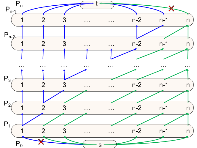
Figure 4. A network with $n^{2}+2$ nodes and a $q$-stable coloring with $q=1$. The maximum flow is $2$, because there exists a cut of size 2 (the blue lower left and green upper right edges). The maximum uniform flow of the bipartite graph induced by $P_{i-1}$ and $P_{i}$, for $i=2,n-1$, is 0, hence $\hat{c}_{1}=0$. The capacity between any two consecutive colors is $n$ or $n+1$ respectively, hence $\hat{c}_{2}(i-1,i)\geq n$.

Example 6.

Consider the network in Figure 4, where each edge has capacity 1. The maximum flow is $2$, because there exists a cut with only two edges (lower left edge, and upper right edge in the figure). The figure shows a coloring that is $q$-stable, for $q=1$; in other words this is a “good” quasi-stable coloring, as close as it can get to a stable coloring. Let’s examine the upper and lower bounds in Theorem 5. On one hand, $\hat{c}_{2}(i-1,i)=n+1$ for $i=2,n-1$, and $\hat{c}_{2}(0,1)=\hat{c}_{2}(n-1,n)=n$. Therefore, the upper bound given by the theorem is $n$, which is a huge overestimate. The reason is that the maximum uniform flow from $P_{i-1}$ to $P_{i}$ is 0. For example, if $f$ is a uniform flow from $P_{1}$ to $P_{2}$, then $f(1,1)+f(1,2)=f(2,3)$ (uniformity at nodes $1,2\in P_{1}$) and $f(1,1)=f(1,2)=f(2,3)$ (uniformity at nodes $1,2,3\in P_{2}$), which implies $f=0$.

Despite this negative example, we show that, under some reasonable assumptions, the two bounds in the theorem can be guaranteed to be close:

Lemma 7.

Let $G=(X,Y,c)$ be a bipartite graph, with capacity $c(x,y)\geq 0$. Let $a,b>0$ be two numbers such that, for all $x\in X$, $c(x,Y)\geq a$ and for all $y\in Y$, $c(X,y)\geq b$, and denote by $F\stackrel{{\scriptstyle\text{def}}}{{=}}\min(a\cdot|X|,b\cdot|Y|)$. Assume that for any two sets of nodes $S\subseteq X$, $T\subseteq Y$, the following holds:

(10) $$c(S,T)+F\geq a\cdot|S|+b\cdot|T|$$

Then $\texttt{maxUFlow}(G)=F$.

We prove the lemma in Appendix A. Here, we show an application. A bipartite graph $G=(X,Y,c)$ is $(a,b)$-biregular if $c(x,Y)=a$ and $c(X,y)=b$ for all $x,y$. We show:

Corollary 8.

(1) If $G$ is an $(a,b)$-biregular graph, then condition (10) holds. (2) If $\bm{P}$ is stable coloring of a network $G$, then $\hat{c}_{1}=\hat{c}_{2}$ and the two bounds in Theorem 5 are equal.

Proof.

(1) In a biregular graph, the quantity $F$ defined in the lemma is $F=\min(a\cdot|X|,b\cdot|Y|)=a\cdot|X|=b\cdot|Y|=c(X,Y)$, and:

$$\begin{array}[]{ll}\lx@intercol F=c(S,T)+c(S,Y-T)+c(X-S,T)+c(X-S,Y-T)\hfil\lx@intercol\\ a\cdot|S|=c(S,T)+c(S,Y-T)&b\cdot|T|=c(S,T)+c(X-S,T)\end{array}$$

Condition (10) simplifies to $c(X-S,Y-S)\geq 0$, which is true since all edge capacities are $\geq 0$.

(2) If $\bm{P}$ is a stable coloring of a network, then every bipartite graph $(P_{i},P_{j},c)$ is $(a,b)$-biregular for some $a,b$ and, furthermore $\hat{c}_{1}(i,j)=\texttt{maxUFlow}(P_{i},P_{j},c)=a\cdot|X|=c(P_{i},P_{j})=\hat{c}_{2}(i,j)$, proving the claim. ∎

4.3. Centrality

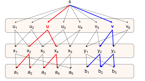
Figure 5. The two nodes $u$ and $v$ have the same color, but different betweenness centrality values: $\color[rgb]{1,0,0}g(u)=6\color[rgb]{0,0,0},\color[rgb]{0,0,1}g(v)=5$.

Finally, we consider the betweenness centrality in a graph and show two results. The first is negative, showing that, even if we compute a stable coloring, nodes with the same color may have different centrality values. The second is positive, assuming we compute the 2-WL coloring instead of 1-WL.

The betweenness centrality is a measure of influence for graph vertices (Freeman, 1977). The betweenness centrality of a vertex $v$ is defined as:

(11) $$g(v)\stackrel{{\scriptstyle\text{def}}}{{=}} \sum_{s,t\mathrel{\mathop{\ordinarycolon}}s\neq v\neq t\neq s}\frac{\sigma(s,t\mid v)}{\sigma(s,t)}$$

over all vertices $s,t$, where $\sigma(s,t)$ is the number of shortest paths between $s,t$ and $\sigma(s,t\mid v)$ is the number of those that pass through $v$.

We usually need to compute the centrality vector, consisting of the values $g(v)$, for all nodes $v$. To speed up this computation, we first compute a quasi-stable coloring, then assume that all nodes of in the same color have the same centrality value: this reduces the cost of the computation, since we only need to compute (11) once for each color (by randomly sampling some $v$ in that color). The question is how reasonable is the assumption that nodes with the same color have similar centrality values.

We observe that, even if the coloring is stable, two nodes $u,v$ of the same color do not necessarily have the same centrality value. This is shown in Fig. 5, where nodes $u$ and $v$ have the same color, but their centrality values differ.

However, we prove a positive result that still justifies our heuristics. Recall that the stable coloring consists of a partition of the nodes of the graph, also called the 1 Weisfeiler-Lehman method, or 1-WL. We prove that, if two nodes are equivalent under the 2-WL equivalence, then they have the same centrality value. We refer the reader to (Morris et al., 2021b, pp.9) for the definition of 2-WL (and, more generally, of k-WL), but instead use the following beautiful characterization of k-WL proved by Cai, Fürer, and Immerman (Cai et al., 1992, Th.5.2), which we review here in a slightly simplified form:

Theorem 9.

Let $C^{k+1}$ be the logic obtained by (a) extending First Order Logic with counting quantifiers of the form $\exists^{\geq m}x\varphi$, which means “there are at last $m$ distinct values $x$ that satisfy $\varphi$”, and (b) restricted to use only $k+1$ variables. Then two nodes $a,b$ in a graph have the same $k$-WL color iff they satisfy the same $C^{k+1}$ formulas.

We prove in Appendix A:

Theorem 10.

Let $u,v$ be two nodes in a graph that have the same 2-WL color. Then they have the same centrality.

We anticipate further applications for our compression. Promising problems to approximate are those whose solutions are robust to edge perturbations, capturing graph-wide properties, including: clustering, node embedding, and computing graph layouts.

5. Algorithm

We have defined two variants of quasi-stable colorings, which allow us to trade off the degree of stability (e.g. by varying $q$ or $\varepsilon$) for the compression ratio (number of colors). It turns out that computing a quasi-stable coloring is more difficult than computing the traditional stable coloring, for both variants. We will describe the challenge first, then introduce our proposed algorithm.

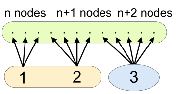
Figure 6. A graph with two maximal q-colorings, for $q=1$, or two maximal $\varepsilon$-relative coloring, for $\varepsilon=1/n$. All nodes at the top are in the same color (green) since all have exactly one incoming edge. The nodes at the bottom can be partitioned into either $\mathinner{\left\{1,2\right\}}$ and $\mathinner{\left\{3\right\}}$ (as shown) or $\mathinner{\left\{1\right\}}$ and $\mathinner{\left\{2,3\right\}}$. Both are maximal 1-stable colorings (because the degrees of two nodes differ by at most 1), and also $1/n$-relative colorings (because the relative error is at most $(n+1)/n\leq e^{1/n}$).

5.1. Complexity

The notion of stable coloring has the elegant property that every graph has a unique, maximal stable coloring. We show here that this property fails for quasi-stable. We use standard terminology from partially ordered sets and call a valid coloring maximal when no valid coarsening exists, i.e. it cannot be greedily improved, and call it maximum or greatest element when it is a coarsening of all valid colorings. Equivalently, a valid coloring is maximum if and only if it is the unique maximal valid coloring. Consider the graph in Fig. 6: there are two distinct maximal 1-stable colorings, and also two distinct $1/n$-relative colorings, because we can partition the nodes $1,2,3$ either as $\mathinner{\left\{1,2\right\}},\mathinner{\left\{3\right\}}$ or as $\mathinner{\left\{1\right\}},\mathinner{\left\{2,3\right\}}$, but cannot leave them in the same color. In fact, we prove:

Theorem 1.

(1) If $\sim$ is a congruence w.r.t. addition (i.e. an equivalence relation satisfying $x\sim y\Rightarrow(x+z)\sim(y+z)$) then any graph admits a unique maximum $\sim$quasi stable coloring, which can be computed in PTIME. (2) Computing a maximal q-stable coloring is NP-complete, and similarly for an $\varepsilon$-stable coloring.

For a simple illustration, fix $c\geq 0$ and define $x\sim y$ if $\min(x,c)=\min(y,c)$; then $\sim$ is a congruence. The theorem implies that there is a unique maximal $\sim$quasi stable coloring. When $c=1$ then this is the maximal bisimulation, and when $c=\infty$ then it is the stable coloring.

The theorem implies that while finding a quasi-stable coloring is trivial (a unique color per node suffices), finding a coloring that cannot be improved is difficult. The question of the practicality of finding a “good enough” coloring is addressed in subsection 5.2.

Proof.

(1) Assume $\sim$ is a congruence. We first prove that, if $\bm{P},\bm{Q}$ are $\sim$-stable colorings of a graph, then so is $\bm{P}\vee\bm{Q}$. A color $C$ of $\bm{P}\vee\bm{Q}$ can be characterized in two ways: (a) for any two nodes $x,x^{\prime}\in C$, there exists a sequence $x_{0}\mathrel{\mathop{\ordinarycolon}}=x,x_{1},x_{2},\ldots,x_{n}\mathrel{\mathop{\ordinarycolon}}=x^{\prime}$ such that every pair $(x_{i-1},x_{i})$ is either in the same color of $\bm{P}$, or the same color of $\bm{Q}$, and (b) $C$ is both a disjoint union of $\bm{P}$-colors, and a disjoint union of $\bm{Q}$-colors, and is minimal such. Let $C,D$ be two colors of $\bm{P}\vee\bm{Q}$, let $x,x^{\prime}\in C$, let $w=w(x,D),w^{\prime}=w(x^{\prime},D)$ be their outgoing weights to $D$, and let $x_{0}\mathrel{\mathop{\ordinarycolon}}=x,x_{1},x_{2},\ldots,x_{n}\mathrel{\mathop{\ordinarycolon}}=x^{\prime}$ be the sequence given by (a). Fix $i=1,n$, and assume w.l.o.g. that $x_{i-1},x_{i}$ have the same $\bm{P}$-color. Then we use the fact that $D$ is a union of $\bm{P}$-colors, $D=P_{j_{1}}\cup\cdots\cup P_{j_{k}}$, and observe that $w(x_{i-1},D)=w(x_{i-1},P_{j_{1}})+\cdots+w(x_{i-1},P_{j_{k}})$ and $w(x_{i},D)=w(x_{i},P_{j_{1}})+\cdots+w(x_{i},P_{j_{k}})$. Since $\bm{P}$ is $\sim$-stable, we have $w(x_{i-1},P_{j_{\ell}})\sim w(x_{i},P_{j_{\ell}})$ for all $\ell$, which implies $w(x_{i-1},D)\sim w(x_{i},D)$ because $\sim$ is a congruence. Finally, we derive $w(x,D)=w(x^{\prime},D)$ because $\sim$ is transitive. Thus proves the claim that $\bm{P}\vee\bm{Q}$ is $\sim$stable. Finally, let $\bm{P}_{1},\bm{P}_{2},\ldots$ be all $\sim$stable colorings. Then $\bm{P}_{1}\vee\bm{P}_{2}\vee\cdots$ is the unique maximum $\sim$stable coloring, and can be computed in PTIME using color refinement.

(2) By reduction from the 2-dimensional Geometric Set Cover problem, more specifically from BOX-COVER, which is NP-complete (Fowler et al., 1981): we are given a set of points $S=\mathinner{\left\{(a_{1},b_{1}),\ldots,(a_{n},b_{n})\right\}}\subseteq\mathbb{R}^{2}$, with integer coordinates, and are asked to cover it with a minimum number of squares with a fixed width $q$. Given this instance of BOX-COVER, we construct the following 3-partite graph $(X,Y,Z,E)$. All edges go from $X$ to $Y$ or from $Y$ to $Z$. The set $Y$ has $n$ nodes. Each node $y_{i}\in y$ has exactly $a_{i}$ incoming edges from $X$, and exactly $b_{i}$ outgoing edges to $Z$: thus $|X|=\sum_{i}a_{i}$ and $|Z|=\sum_{i}b_{i}$. Any $q$-stable coloring of the graph corresponds to a cover of $S$ with $q\times q$ squares. ∎

5.2. Rothko Algorithm

Given the negative results above, we settle for a heuristic-based algorithm for finding quasi-stable colorings that may not be maximal. The main idea is that, instead of imposing some $q$, the algorithm repeatedly applies a variant of color refinement, until a maximum number of colors is reached. The value of $q$ is the computed on this coloring. The guarantees given by the theorems in Sec. 3 still hold on the resulting colored graph, but the quality of the approximation depends on how good the value $q$ is when the algorithm terminates. We briefly describe the algorithm next.

We call the algorithm Rothko and list it in Algorithm 1. The name reflects its method of dividing matrices into a few large, rectangular regions and giving them distinct colors—resembling Rothko’s famous color field paintings.

This iterative algorithm operates by refining one color at a time, beginning with the coarsest (i.e., single color) partition. At every step a witness is identified: that is, the pair of partitions $P_{i},P_{j}$ that maximize error in the $P_{i}\rightarrow P_{j}$ direction. The source color is then split into $P_{i}^{\prime},P_{i}^{\prime\prime}$ to reduce the sum of errors $P_{i}^{\prime}\rightarrow P_{j}$ and $P_{i}^{\prime\prime}\rightarrow P_{j}$. This process is repeated until the desired error bound or number of colors is reached.

A witness is identified by calculating the maximum, minimum degrees between all colors ($U,L$ respectively) and taking the difference of the two matrices. This produces the error matrix $Err=U-L$, whose $(i,j)$^th entry records the q-error of color $P_{i}$ with respect to $P_{j}$. Then, a threshold is set by taking the mean degree into $P_{j}$ of the nodes in $P_{i}$. The elements of $P_{i}$ are then split depending on whether their degree exceeds this threshold. We break ties arbitrarily–notice if we have a tie, often at the next around we will split the other tied-with color. We find ties to be rare in our experiments.

For some applications, it is desirable to weight the error by the size of the partition, so that a q-error in a large partition is considered worse than a q-error in a small partition. As such, the algorithm accepts two parameters, $\alpha,\beta$ which allow for building a weight matrix $C$. These parameters control the weight assigned to the source and target colors, respectively. $C$ is multiplied element-wise by $E$ to produce the weighted error matrix $E_{weighted}$. In practice, we set $\alpha=\beta=0$ for max-flow problems, as neither the number of source nor target nodes affects the flow, but only the total edge capacity between the colors; for linear programs, $\alpha=1,\beta=0$ which prioritizes colors with more rows; for betweenness centrality, $\alpha=\beta=1$ as the number of paths depends on both the number of nodes in source and target color.

Further, for applications where all weights are non-negative, we observe that using the geometric rather than arithmetic mean results in a more compact coloring. The intuition can be gleaned from scale-free networks, where the proportion of nodes with degree $k$ tends is proportional to $k^{-\gamma}$. Under the most common scale-free model, Barabási–Albert (Barabási and Albert, 1999), where $\gamma=3$ and the average degree is $2m$, splitting using arithmetic mean yields unbalanced partitions with $1/(8m^{3})$ fraction of nodes. Even for modest values of $m$ this quickly becomes unbalanced (i.e. when $m=3$ the partition will be split $1\mathrel{\mathop{\ordinarycolon}}216$). Since the geometric mean is equivalent to the arithmetic mean in log-space, the split is much less unbalanced (in the previous example, it would be $1\mathrel{\mathop{\ordinarycolon}}4$). Many natural networks—such as the internet—are thought to be scale-free (Barabási, 2013).

Data: $G=(V,E),W\mathrel{\mathop{\ordinarycolon}}V\times V\rightarrow\mathbb{R}^{+}$

Parameters: $n\in\mathbb{Z}^{+},\varepsilon\in\mathbb{R}_{\geq 0},~{}\alpha,\beta\in\mathbb{R}$

Result: $P\subset\mathcal{P}(V)$

3 $P\leftarrow\mathinner{\left\{V\right\}}$;

4 while $|P|<n$ do

5       $U_{ij},L_{ij}\leftarrow\max_{v\in P_{i}}\text{deg}(v,P_{j}),\min_{v\in P_{i}}\text{deg}(v,P_{j})$;

6       $Err\leftarrow U-L$;

7       if $\max Err\leq\varepsilon$ then

8            break;

9      $C_{ij}\leftarrow|P_{i}|^{\alpha}\times|P_{j}|^{\beta}$; // weights

10       $Err_{\text{weighted}}\leftarrow Err\odot C$; // element-wise product

11       $i,j\leftarrow\operatorname*{argmax}_{i,j}Err_{\text{weighted}}$; // witness

12       $\text{threshold}\leftarrow\text{mean}(\mathinner{\left\{x\mid x=\text{deg}(v,P_{j}),v\in P_{i}\right\}})$ ;

       // Split $P_{i}$ at threshold

13       $P_{\text{retain}}\leftarrow\mathinner{\left\{v\in P_{i}\mid\text{deg}(v,P_{j})\leq\text{threshold}\right\}}$;

14       $P_{\text{eject}}\leftarrow P_{i}\setminus P_{\text{retain}}$;

15       $P\leftarrow P\setminus\mathinner{\left\{P_{i}\right\}}\cup\mathinner{\left\{P_{\text{retain}},P_{\text{eject}}\right\}}$;

16      

Computing an approximate partition over a weighted graph $G$, with $n$ colors or $\varepsilon$ maximum $q$-error

Algorithm 1 Rothko

Computing an approximate partition over a weighted graph $G$, with $n$ colors or $\varepsilon$ maximum $q$-error

Rothko is an anytime algorithm. It can be interrupted and will still produce in a valid coloring. The longer it is allowed to run, the better the resulting coloring is. Further, the stopping condition can be set depending on a desired number of colors, or target $q$-error, encoded in Algorithm 1 as $n,\varepsilon$ respectively. This is particularly valuable in interactive applications, where Rothko can be run as a co-routine, with the application alternating between color refinement and updating its approximation based on the new colors.

This algorithm is guaranteed to terminate. At each iteration, a color is chosen to be split. Singleton colors are never selected for splitting, as their degree-difference into any partition is zero. As such, after enough iterations either the algorithm will reach its desired error bound, or have refined into the trivial partitioning—consisting of only singleton partitions and so a maximum $q$-error of zero.

6. Evaluation

We empirically evaluate our notion of quasi-stable coloring, addressing three questions:

1. End-to-end performance: how good is the system downstream? Can it effectively trade-off accuracy for speedup?

2. What are the characteristics of the colors? What are the properties of the compressed graphs?

3. How efficient and scalable is the Rothko algorithm?

We use 20 datasets for evaluation. Graphs are outlined in Table 2, linear programs in Table 3. We list the primary sources in the table, many of these graphs were found via dataset repositories (Leskovec and Krevl, 2014; wat, 2013). Trials are run on a MacOS machine with a 3.2 GHz ARMv8 processor and 16GB of main memory. A single core is used for all experiments. All code is run on Julia v1.7, with linear programs being solved with the Tulip solver and max-flow problems with the GraphsFlows library. Tulip is the fastest open-source solver (Tanneau et al., 2021), while GraphsFlows uses the state-of-the-art push-relabel algorithm (Goldberg, 2008). Our coloring implementation, as tested in this paper, is packaged as QuasiStableColors version v0.1.0 and is available for download.

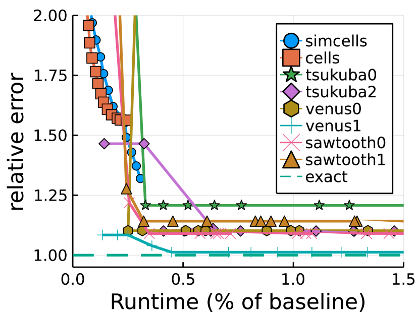
(a) Maximum-flow

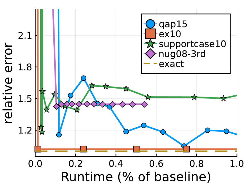
(b) Linear optimization

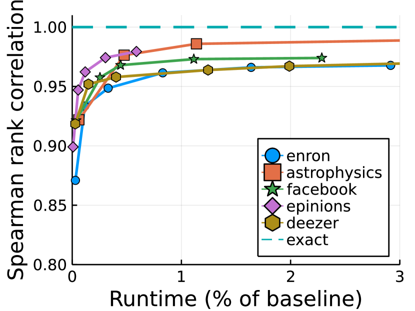
(c) Centrality

Figure 7. Speed-accuracy trade-offs for three task types and 20 datasets. Runtime reported is end-to-end, including the time taken for graph coloring, building an approximate instance of the problem and solving it.

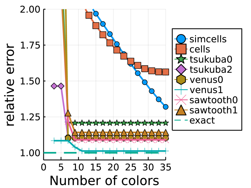
(a) Maximum-flow

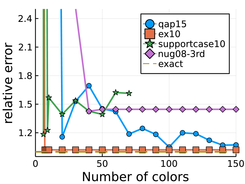
(b) Linear optimization

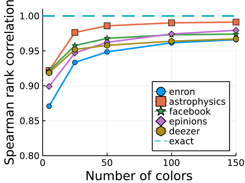
(c) Centrality

Figure 8. Accuracy as a function of the number of colors, across the same three tasks.

Table 1. Runtime comparison of q-stable colors vs. prior approximations (Riondato-Kornaropoulos (Riondato and Kornaropoulos, 2014) and early-stopping (OR-Tools, [n.d.])) and exact algorithms (Brandes (Brandes, 2001) and interior-point solver (Tanneau et al., 2021)). Runtime to achieve a target approximation quality is measured; target is correlation ($\rho$) with ground truth values for centrality and relative error for linear optimization. “$\times$” is 20-minute timeout. Units in seconds, lower is better.

	Betweenness centrality: ours, (Riondato and Kornaropoulos, 2014), and (Brandes, 2001)
	$\rho=0.90$		$\rho=0.95$		$\rho=0.97$		Exact
	Ours	Prior	Ours	Prior	Ours	Prior
Astroph.	0.13	15.2	1.03	41.4	2.49	61.1	223
Facebook	0.07	3.2	0.53	7.1	2.23	12.6	221
Deezer	0.05	3.6	1.11	7.2	8.56	14.8	295
Enron	0.41	2.6	3.06	5.6	10.8	8.7	380
Epinions	0.18	17.1	3.15	36.5	7.95	58.2	2552
	Linear optimization: ours, (OR-Tools, [n.d.]), and (Tanneau et al., 2021)
	$\text{rel. err.}=3.0$		$\text{rel. err.}=2.0$		$\text{rel err.}=1.5$		Exact
	Ours	Prior	Ours	Prior	Ours	Prior
qap15	3.20	112.	4.91	524.	11.4	$\times$	1 320
nug08.	5.40	1 027.	6.65	$\times$	6.65	$\times$	6 000
support.	0.51	143.	4.98	143.	$\times$	$\times$	1 860
ex10	0.247	795.	14.0	795.	14.0	795.	1 440

Table 2. Summary of graphs used for evaluation

Name	Vertices	Edges	Real/ Sim.	Source
General evaluation
Karate	34	75	R	(Girvan and Newman, 2002)
OpenFlights	3 425	38 513	R	(Patokallio, 2014)
Dblp	317 080	1 049 866	R	(dblp team, [n.d.])
Centrality
Astrophysics	18 772	198 110	R	(Leskovec et al., 2007)
Facebook	22 470	171 002	R	(McAuley and Leskovec, 2012)
Deezer	28 281	92 752	R	(Rozemberczki and Sarkar, 2020)
Enron	36 692	183 831	R	(Klimt and Yang, 2004)
Epinions	75 879	508 837	R	(Richardson et al., 2003)
Maximum-flow
Tsukuba0	110 594	506 546	R	(of Tsukuba, 2001)
Tsukuba2	110 594	500 544	R	(of Tsukuba, 2001)
Venus0	166 224	787 946	R	(Scharstein and Szeliski, 2002)
Venus1	166 224	787 716	R	(Scharstein and Szeliski, 2002)
Sawtooth0	164 922	790 296	R	(Scharstein and Szeliski, 2002)
Sawtooth1	164 922	789 014	R	(Scharstein and Szeliski, 2002)
SimCells	903 962	6 738 294	S	(Jensen et al., 2020)
Cells	3 582 102	31 537 228	R	(Jensen et al., 2020)

Table 3. Summary of the linear programs used for evaluation. All instances are from real problems.

Name	Rows	Cols.	Non-zeros	Sol. time	Source
qap15	6 331	22 275	110 700	22 min	(Mittelmann, 2022)
nug08-3rd	19 728	20 448	139 008	100 min	(Mittelmann, 2022)
supportcase10	10 713	1 429 098	4 287 094	31 min	(Mittelmann, 2022)
ex10	69 609	17 680	1 179 680	24 min	(Mittelmann, 2022)

Table 4. Runtime and compression ratios of quasi-stable coloring vs. prior work (stable coloring (L. Staudt et al., 2016; Berkholz et al., 2017)) for selected datasets.

Dataset	Max $q$	Mean $q$	Colors	Compression	Time
OpenFlights	stable ($q=0$)		2 637	1.29:1	150ms
	q = 64	15.8	9	380:1	10ms
	q = 32	6.96	17	200:1	20ms
	q = 16	2.22	39	87:1	60ms
	q = 8	0.52	106	32:1	350ms
Epinions	stable ($q=0$)		53 068	1.42:1	49s
	q = 64	4.42	71	1 000:1	2.39s
	q = 32	1.17	144	526:1	8.95s
	q = 16	0.79	316	240:1	40.5s
	q = 8	0.22	869	87:1	5m19s
DBLP	stable ($q=0$)		233 466	1.35:1	14m52s
	q = 64	11.94	21	15 000:1	2.28s
	q = 32	2.22	89	3 500:1	22.6s
	q = 16	0.39	373	850:1	6m39s
	q = 8	0.06	1513	210:1	2h38m

6.1. End-to-end performance

In this section, we consider how well q-stable colors work as a function of downstream performance. We evaluate the trade-off between accuracy and speed when using the colorings for approximating linear-optimization, maximum-flow, and centrality tasks. On all tasks, we compare against the baseline of solving the problem directly on the graph or linear system.

For maximum-flow and linear-optimization tasks, we use the relative error as the performance metric. We define this as $\max(v/\hat{v},\hat{v}/v)$ for an actual, predicted $v,\hat{v}$ so that $1.0$ is the ideal score. For betweenness centrality, the actual and predicted scores are compared pair-wise using Spearman’s rank correlation coefficient, where $1.0$ is also the ideal score. In all experiments, the time reported is end-to-end i.e., includes coloring the graph or matrix, computing the reduced problem, and solving it.

Figure 7 illustrates the trade-off for three task types across twenty datasets. Overall, accuracy can be exchanged for speed favorably: in the average case, using a budget of $1\%$ of the baseline (i.e., a $100\times$ speedup) results in an average error within $12\%$ of the optimal value. Figure 8 shows the number of colors required to achieve the same accuracy. Across all tasks, no more than 150 colors are required to converge to an approximation. We observe a consistent diminishing-returns pattern: the initial color refinement results in large gains in accuracy, but as more and more colors are added the gains shrink in size. Comparing the densities of the graphs (omitted for brevity) with the difficulty of coloring them, we find no consistent trend. Next, we consider the tasks individually.

Maximum Flow

We test our algorithm on problem instances defined by min-cut/max-flow benchmarks (Jensen et al., 2021; wat, 2013). This involves computing maximum flows over the eight flow networks. We compare against a baseline of computing the exact flow using the push-relabel algorithm, considered to be the benchmark for max-flow (Goldberg, 2008).

Figure 7(a) shows the results: our approximation achieves an average geometric-mean error of $1.17$ while using less than $1\%$ of the time needed for direct solution. At the same time, as outlined in Figure 8(a), this error is achieved using no more than $35$ colors. Recall that the flow networks are composed of 100K-2M nodes.

We consider comparing with prior approximation algorithms. The state-of-the-part push-relabel algorithm for max-flow cannot be stopped early, as it computes pre-flows which are not valid flows and violate the principle of flow conservation. Further, while linear-time approximations have been developed in the theory (Kelner et al., 2014), these algorithms remain slower than push-relabel algorithm in practice.

Linear programs

Next, we evaluate the ability of quasi-stable coloring to approximate solutions to linear systems of equations. We test on four real-world linear programs, outlined in Table 3. These are relatively difficult tasks: the easiest can be solved in 20 minutes while the most difficult requires about two hours for an exact solution.

$q$-stable colors provide a good speed-accuracy tradeoff, shown in Figure 7(b). On average, a geometric-mean relative-error of $1.13$ is reached in under $0.5\%$ of the direct runtime. Figure 8(b) shows the number of colors required for the results. Similarly to max-flow, a relatively small number of colors is required for an accurate answer. Unlike other tasks, the error on LPs is not monotone.

Table 1 (bottom) compares our approximation with early stopping the interior-point-method solver, the recommended approach in practice (OR-Tools, [n.d.]). We set a relative error and solve until that bound is met. Q-stable coloring outperforms the baseline runtime by $10^{2}\times$ on average and times out in only one configuration (vs. five).

Centrality

Next, we test the utility of q-stable colorings in approximating betweenness centrality. We measure the approximation error using Spearman’s rank correlation coefficient. We compare against the baseline of solving for exact centralities using Brandes algorithm (Brandes, 2001), the algorithm with the best asymptotic runtime.

Figure 7(c) shows the speedup-accuracy tradeoff on five medium-size datasets. On all datasets, the approximation is favorable: using $1\%$ of the time of the direct computation, it produces centralities with correlation $0.973$ to the ground truth. Figure 8 outlines the number of colors required for these results. We find that using 50 colors is sufficient to ensure a rank correlation of greater than $0.948$, while 100 colors allow for $0.965$. Recall the graphs have 18–75K vertices. We exclude the datasets dblp and larger because the baseline timed out after 16 hours.

We note a few trends. First, the speed-accuracy trade-off is more favorable the larger the dataset. The largest dataset, epinions, shows the steepest slope at the beginning; the dataset with the fewest vertices, Astrophysics, shows the shallowest slope. As with maximum-flow, the approximation error is found to be monotone over all datasets: the more colors used, the better the correlation is.

Table 1 (top) compares the performance of our approximation with prior works (Riondato and Kornaropoulos, 2014). By compressing all nodes in the graph rather than focusing on selecting paths to sample, we obtain a $30\times$ better average runtime across various tasks and approximation budgets.

6.2. Coloring Characteristics

Coloring size

Table 4 compares the q-stable coloring of three datasets with stable coloring. Stable coloring results in compressed graphs with $70\%$-$78\%$ of the full graph size. We find that small maximum values of $q$, such as $q=8$ result in an order-of-magnitude improvement in the compression ratios over stable coloring. Moderate maximum values of $q$, such as $q=16$ result in a two or more orders-of-magnitude improvement. While the choice of $q$ caps the worst-case degree error, the average errors are much smaller, on average $<1.0$ on all datasets: less than one differing edge per color.

Color distribution

Unlike stable coloring, single-element partitions do not dominate any dataset. For example, on cells, DBLP, nug08-3rd and epinions, the median partition contains 6, 14, 56, 206 nodes in each dataset respectively. This evidences the ability of $q$-stable colors to avoid stable-coloring-like single-color partitions.

Table 5. Characteristics of the constraint matrix for some compressed linear programs.

Dataset	Colors	Rows	Cols.	Non-zeros	Comp-ression ratio	Rel. error
qap15	10	4	7	11	$10^{4}$	18.91
	50	27	24	179	$10^{3}$	1.45
	100	52	49	478	$10^{2}$	1.05
nug08-3rd	5	3	3	5	$10^{4}$	8.19
	50	30	21	254	$10^{3}$	1.45
	100	61	40	930	$10^{3}$	1.45
supportcase10	5	3	3	4	$10^{5}$	$10^{10}$
	50	30	21	131	$10^{3}$	1.39
	100	62	39	368	$10^{3}$	1.51
ex10	5	5	1	4	$10^{6}$	5.28
	50	25	26	347	$10^{3}$	1.02
	100	51	50	864	$10^{3}$	1.02

Compression ratios

Table 5 shows the compression ratios enabled by using quasi-stable colors on linear programs. A maximum compression of $10^{6}\times$ is recorded, but corresponds to a large error of 5.28. Typical space savings of a ratio of $10^{2}$-$10^{3}$ while maintaining a geometric mean error of $1.23$. The outlier error of $10^{10}$ on supportcase10 is explained by the measured q-error of $10^{7}$ when only 5 colors are used–this sharply decreases with more colors.

6.3. Algorithm Properties

Table 6. Average latency and responsiveness of the Rothko algorithm across task types.

Task	Time-to-first-result	Update frequency	Time to converge
Linear opt.	560 ms	2.71 s	72.2 s
Max-flow	845 ms	1.57 s	21.0 s
Centrality	32 ms	1.60 s	5.88 s

Runtime

Table 4 compares runtime against the state-of-the-art stable-coloring algorithm (Berkholz et al., 2017) with complexity $\mathcal{O}((n+m)\log n)$. Rothko’s runtime is competitive against this highly optimized implementation (L. Staudt et al., 2016), with an order-of-magnitude better compression.

Responsiveness

Because of the progressive nature of the Rothko algorithm, an initial prediction is produced promptly. Table 6 outlines the latency and responsiveness metrics. The first prediction occurs within 480 ms on average, with centrality tasks having the consistently lowest latency and max-flow the highest. Average latency is strongly influenced by outliers, such as cells with 6.5s of latency. Further, the algorithm iterates well, with a new color computed every $1.96s$ on average. The time taken for the subtasks varies: for max-flow and linear-program problems, the coloring step dominates, using $>99.9\%$ of the runtime on the measured datasets. For centrality the solving step dominates, taking up $68\%$–$94\%$ of the runtime.

Robustness

We compare the robustness of q-colors to graph perturbations against that of stable coloring. We construct a synthetic graph $|V|=1000,E=|21~{}600|$ with a compact, 100-color stable coloring. Then in Figure 2, a small number of edges is added at random. The initial stable coloring has a compression ratio of $10\times$. Perturbing $1.5\%$ of edges causes the stable coloring to degrade to a compression ratio of 75% (750 nodes, down from 1000), with a majority of nodes given a unique color. Computing a $q$-stable color ($q=4$), the compression ratio can be maintained at $6.5\times$ with the same perturbation.

7. Conclusion

We have introduced quasi-stable colorings, an approach for vertex classification that allows for the lossy compression of graphs. By developing an approximate version of stable coloring, we are able to practically color real-world graphs. We show the ability of these colorings as approximations of max-flow/min-cut, linear optimization and betweenness centrality and prove their error bounds. Discovering that the construction of maximal q-stable colorings is NP-hard, we develop a heuristic-based algorithm to efficiently compute them. We empirically evaluate the characteristics and approximation utility of quasi-stable colors; validating their practicality on wide range of real datasets and tasks.

Appendix A Appendix

Proof of Theorem 1

We prove here Theorem 1. In general, it is well known that ${\mathcal{OPT}}(A,b,c)$ is a continuous function in $A,b,c$. We prove here a stronger statement: if $A,b,c$ is well behaved (see Sec. 4.1), then the function is Lipschitz continuous in $b,c$.

Lemma 1.

Given $A,b,c$ as above, there exists $q_{0}>0$ such that, forall $u\in\mathbb{R}^{m},v\in\mathbb{R}^{n}$, if $||u||_{\infty}\leq q_{0}$ and $||v||_{\infty}\leq q_{0}$, then $|{\mathcal{OPT}}(A,b+u,c+v)-{\mathcal{OPT}}(A,b,c)|=O(||u||_{\infty}+||v||_{\infty})$.

Proof.

Recall that the optimal solution $x^{*}$ can always be chosen to be a vertex of the polytope defined by the LP. More precisely, consider the $m+n$ inequality constraints $Ax\leq b$, $x\geq 0$. Choose any $n$ of them and convert them to equalities; if they uniquely define $x$, then we call $x$ a candidate solution, and we denote by $x_{1},\ldots,x_{N}$ all candidate solutions. Let $x_{i}$ be candidate solution that is feasible and optimal for $A,b,c$, and let $x_{j}$ be the candidate solution that is feasible and optimal for $A,b,c+v$ respectively. Then $|{\mathcal{OPT}}(A,b,c+v)-{\mathcal{OPT}}(A,b,c)|=|v^{T}(x_{j}-x_{i})|\leq||v||_{\infty}||x_{j}-x_{i}||_{1}\leq O(q)$, where the constant in $O(-)$ is $2\max_{i}||x_{i}||_{1}$. By applying the same argument to the dual LP we obtain $|{\mathcal{OPT}}(A,b+u,c)-{\mathcal{OPT}}(A,b,c)|=O(q)$. Returning to the primal LP, we notice that if we replace $b$ with $b+u$, then the candidate solutions $x_{i}$ will change to some $x_{i}^{\prime}$; since $u$ ranges over a compact set, $\sup_{u}||x_{i}^{\prime}||_{1}$ exists and is finite, for all $i=1,N$, which implies $|{\mathcal{OPT}}(A,b+u,c+v)-{\mathcal{OPT}}(A,b+u,c)|=O(q)$. Thus, $|{\mathcal{OPT}}(A,b+u,c+v)-{\mathcal{OPT}}(A,b,c)|=O(q)$ as required. ∎

Using the lemma, we can now prove Theorem 1. Define:

(12) $$\bm{U}(r,i)\stackrel{{\scriptstyle\text{def}}}{{=}} \frac{\bm{1}_{i\in P_{r}}}{\sqrt{|P_{r}|}} \bm{V}(s,j)\stackrel{{\scriptstyle\text{def}}}{{=}} \frac{\bm{1}_{j\in Q_{s}}}{\sqrt{|Q_{s}|}}$$

where $\bm{1}_{\pi}$ is the indicator function of a predicate $\pi$, equal 1 when $\pi$ is true, and equal 0 otherwise. $\bm{U}$ and $\bm{V}$ represent mappings between the original LP and the reduced LP, and we will show that they satisfy a relaxed version of Eq. (9). Observe that the last row and last column of both $\bm{U}$ and $\bm{V}$ are $0,0,\ldots,0,1$, and denote by $U,V$ (without boldface) the matrices obtained by removing the last row and last column. Then $\hat{A}=UAV^{T}$, $\hat{b}=Ub$, and $\hat{c}^{T}=c^{T}V^{T}$ (see their definitions in Eq. (8)). Next, we define the following matrices $\bm{D},\bm{E}$, which capture the error introduced by the mapping from $A,b,c$ to $\hat{A},\hat{b},\hat{c}$. We also show them as block matrices, by exposing the last row and last column:

$$\bm{D}\stackrel{{\scriptstyle\text{def}}}{{=}}\bm{A}\bm{V}^{T}-\bm{U}^{T}\hat{\bm{A}}= \bm{E}\stackrel{{\scriptstyle\text{def}}}{{=}}\bm{U}\bm{A}-\hat{\bm{A}}\bm{V}=$$

(23) $$\left(\begin{array}[]{ c |c}&d_{1}\mathrel{\mathop{\ordinarycolon}}=\\ &b\\ D\mathrel{\mathop{\ordinarycolon}}=AV^{T}-U^{T}\hat{A}&-\\ &U^{T}\hat{b}\\ \hline\cr c^{T}V^{T}-\hat{c}^{T}=0&0\end{array}\right) \left(\begin{array}[]{ c |c}&Ub\\ &-\\ E\mathrel{\mathop{\ordinarycolon}}=UA-\hat{A}V&\hat{b}\\ &=0\\ \hline\cr e_{2}^{T}\mathrel{\mathop{\ordinarycolon}}=c^{T}-\hat{c}^{T}V&0\end{array}\right)$$

We show that the error matrices are small:

(24) $$|\bm{D}(s,i)|\leq \frac{q}{\sqrt{|Q_{s}|}} |\bm{E}(r,j)|\leq\frac{q}{\sqrt{|P_{r}|}}$$

We only show the first inequality, the second is identical:

$$\bm{D}(s,i)= \sum_{j}\frac{\bm{A}(i,j)\bm{1}_{j\in Q_{s}}}{\sqrt{|Q_{s}|}}-\sum_{r}\frac{\bm{1}_{i\in P_{r}}\hat{\bm{A}}(r,s)}{\sqrt{|P_{r}|}}$$

$$= \frac{\bm{A}(i,Q_{s})}{\sqrt{|Q_{s}|}}-\frac{\bm{A}(P_{r},Q_{s})}{P_{r}\cdot\sqrt{|Q_{s}|}}=\frac{1}{\sqrt{|Q_{s}|}}\left(\bm{A}(i,Q_{s})-\frac{\bm{A}(P_{r},Q_{s})}{|P_{r}|}\right)$$

where in the last line $r$ is the unique color that contains $i$. The quantity $\bm{A}(i,Q_{s})$ represents the total weight from $i$ to the color $Q_{s}$, while $\bm{A}(P_{r},Q_{s})/|P_{r}|$ is the average of this quantity over all $i\in P_{r}$. Since the coloring is $q$-quasi stable, this difference is bounded by $q$.

For any feasible solution $x$ to the LP (2), define $\hat{x}\stackrel{{\scriptstyle\text{def}}}{{=}}Vx$. Since $Ax\leq b$, we derive $UAx\leq Ub$, which becomes $(\hat{A}V+E)x\leq\hat{b}$, or $\hat{A}Vx\leq\hat{b}-Ex$. Moreover, $c^{T}x=(\hat{c}^{T}V+e_{2}^{T})x=\hat{c}^{T}\hat{x}+e_{2}^{T}x$. It follows that ${\mathcal{OPT}}(A,b,c)\leq{\mathcal{OPT}}(\hat{A},\hat{b}-Ex,\hat{c})+e_{2}^{T}x$. We set $x\mathrel{\mathop{\ordinarycolon}}=x^{*}$ (an optimal solution to the LP) and observe that Eq. (24) implies $||Ex^{*}||_{1}\leq q||x^{*}||_{1}$, and $||e_{2}^{T}x^{*}||_{1}\leq q||x^{*}||_{1}$. Therefore, Lemma 1 implies ${\mathcal{OPT}}(\hat{A},\hat{b}-Ex,\hat{c})\leq{\mathcal{OPT}}(\hat{A},\hat{b},\hat{c})+q\Delta$, for some constant $\Delta$. We have proven that ${\mathcal{OPT}}(A,b,c)\leq{\mathcal{OPT}}(\hat{A},\hat{b},\hat{c})+O(q)$.

Conversely, for $\hat{x}$ any feasible solution to (7), define $x\stackrel{{\scriptstyle\text{def}}}{{=}}V^{T}\hat{x}$. Since $\hat{A}\hat{x}\leq\hat{b}$, we derive $U^{T}\hat{A}\hat{x}\leq U^{T}\hat{b}$, or $(AV^{T}-D)\hat{x}\leq b-d_{1}$, which we rearrange as $Ax\leq b+(D\hat{x}-d_{1})$. Moreover, $c^{T}x=c^{T}V^{T}\hat{x}=\hat{c}^{T}\hat{x}$. It follows that ${\mathcal{OPT}}(\hat{A},\hat{b},\hat{c})\leq{\mathcal{OPT}}(A,b+(D\hat{x}-d_{1}),c)$. We set $\hat{x}\mathrel{\mathop{\ordinarycolon}}=\hat{x}^{*}$ (an optimal solution to the reduced LP), and observe that $||D\hat{x}^{*}-d_{1}||_{1}=O(q)$. Therefore, Lemma 1 implies ${\mathcal{OPT}}(A,b+(D\hat{x}-d_{1}),c)\leq{\mathcal{OPT}}(A,b,c)+q\Delta$, for some constant $\Delta$. This completes the proof of the theorem.

Proof of Lemma 7

We prove here Lemma 7. Extend $G$ to a network by adding two nodes $s,t$ and setting $c(s,x)\stackrel{{\scriptstyle\text{def}}}{{=}}F/|X|$ and $c(y,t)\stackrel{{\scriptstyle\text{def}}}{{=}}F/|Y|$ for all $x\in X,y\in Y$. We claim that this network admits a flow of value $F$. The claim implies that the flow is uniform, since all edges $(s,x)$ and $(y,t)$ must have a flow up to their capacity. To prove the claim it suffices to show that every cut in the network has a capacity $\geq F$. Let $C$ be any cut. Define the sets:

$$S\stackrel{{\scriptstyle\text{def}}}{{=}} \{{x}\mid{x\in X,(s,x)\not\in C}\} T\stackrel{{\scriptstyle\text{def}}}{{=}} \{{y}\mid{y\in Y,(y,t)\not\in C}\}$$

The cut must contain all edges $(x,y)$ with $x\in S$, $y\in T$, hence its capacity is:

$$c(S,T)+\left(|X|-|S|\right)\frac{F}{|X|} +\left(|Y|-|T|\right)\frac{F}{|Y|}$$

$$=\left(c(S,T)+F-|S|\frac{F}{|X|}-|T|\frac{F}{|Y|}\right)+F \geq\left(c(S,T)+F-a\cdot|S|-b\cdot|T|\right)+F\geq F.\quad\square$$

Proof of Theorem 10

We write $d(a,b)$ for the length of the shortest path from $a$ to $b$ in the graph. We claim that, for all numbers $M\geq 0$ and $d\geq 0$, the following formula $\Phi_{M,d}$ can be expressed in $C^{3}$:

$$\Phi_{M,d}(s,v)\stackrel{{\scriptstyle\text{def}}}{{=}} (d(s,v)=d)\wedge(\sigma(s,v)\geq M)$$

The claim implies the theorem, because we can write $g(v)$ as follows. Notice that $\sigma(s,t\mid v)=\sigma(s,v)\sigma(v,t)$ when $d(s,t)=d(s,v)+d(v,t)$ and $\sigma(s,t\mid v)=0$ otherwise. Then:

$$g(v)= \sum_{M_{1},M_{2},M,d_{1},d_{2},s,t}\left\{\frac{M_{1}M_{2}}{M}\mid\Psi_{M_{1},d_{1}}(s,v)\wedge\Psi_{M_{2},d_{2}}(v,t)\wedge\Psi_{M,d_{1}+d_{2}}(s,t)\right\}$$

where $\Psi_{M,d}\stackrel{{\scriptstyle\text{def}}}{{=}}\Phi_{M,d}\wedge\neg\Phi_{M+1,d}$ asserts that $\sigma=M$. The claim implies that, if $u,v$ have the same 2-WL color, then, by Theorem 9, we have $\Phi_{M,d}(s,u)\equiv\Phi_{M,d}(s,v)$ for all $M,d,s$, and similarly $\Phi_{M,d}(u,t)\equiv\Phi_{M,d}(v,t)$, which implies $g(v)=g(u)$. It remains to prove the claim. Recall that, for all $d\geq 0$, the formula $\Pi_{\leq d}(x,y)$ saying “there exists a path of length $\leq d$ from $x$ to $y$” is expressible in $C^{3}$. For example, $\Pi_{\leq 4}(x,y)=\exists z(E(x,z)\wedge\exists x(E(z,x)\wedge\exists z(E(x,z)\wedge E(z,y))))$. Then $\Pi_{=d}(x,y)\stackrel{{\scriptstyle\text{def}}}{{=}}\Pi_{\leq d}(x,y)\wedge\neg\Pi_{\leq(d-1)}(x,y)$ asserts that $d(x,y)=d$. Next, we notice that:

(25) $$\sigma(s,v)=\sum_{w\mathrel{\mathop{\ordinarycolon}}E(w,v)\wedge(d(s,v)=d(s,w)+1)}\sigma(s,w)$$

If $n$ is the number of nodes in the graph, then for each $\ell=1,n$ we denote by $\mathcal{M}_{\ell}$ the set of all strictly increasing $\ell$-tuples of natural numbers $\bm{M}=(M_{1},\ldots,M_{\ell})$, where $0<M_{1}<M_{2}<\cdots<M_{\ell}\leq M$. Similarly, denote by $\mathcal{C}_{\ell}$ the set of all $\ell$-tuples of natural numbers $\bm{c}=(c_{1},\ldots,c_{\ell})$, where $0<c_{i}\leq M$. Then:

$$\Phi_{M,d}(s,w)= \bigvee_{\begin{array}[]{c}\bm{M}\in\mathcal{M};\bm{c}\in\mathcal{C}\\ \sum_{i}c_{i}M_{i}\geq M\end{array}}\bigwedge_{i=1,\ell}\exists^{\geq c_{i}}w\mathrel{\mathop{\ordinarycolon}}\Pi_{=(d-1)}(s,w)\wedge\Psi_{M_{i},d-1}(s,w)$$

In other words, for every combination of numbers $M_{i},c_{i}$ such that $\sum_{i}c_{i}M_{i}\geq M$, the formula checks if, for each $i$, there exists at least $c_{i}$ parents $w$ at distance $d-1$ from $s$, where $\sigma(s,w)=M_{i}$. We prove that the formula is correct. Suppose the RHS is true. Then, for each $i$, there are at least $c_{i}$ distinct nodes $w$ that satisfy the formula $\Pi_{=(d-1)}(s,w)\wedge\Psi_{M_{i},d-1}(s,w)$. For each such $w$, we have $\sigma(s,w)=M_{i}$, and therefore their contribution to the sum in (25) is $c_{i}M_{i}$. Since the numbers $M_{1},\ldots,M_{\ell}$ are distinct, it follows that the set of nodes $w$ associated to distinct values $i$ are disjoint, hence their total contribution to (25) is $\sum_{i}c_{i}M_{i}$, which is $\geq M$ as required.

References

- (1)
- wat (2013) 2013. Max-flow problem instances in vision. https://vision.cs.uwaterloo.ca/data/maxflow
- Barabási (2013) Albert-László Barabási. 2013. Network science. Philosophical Transactions of the Royal Society A: Mathematical, Physical and Engineering Sciences 371, 1987 (2013), 20120375.
- Barabási and Albert (1999) Albert-László Barabási and Réka Albert. 1999. Emergence of scaling in random networks. science 286, 5439 (1999), 509–512.
- Berkholz et al. (2017) Christoph Berkholz, Paul S. Bonsma, and Martin Grohe. 2017. Tight Lower and Upper Bounds for the Complexity of Canonical Colour Refinement. Theory Comput. Syst. 60, 4 (2017), 581–614. https://doi.org/10.1007/s00224-016-9686-0
- Brandes (2001) Ulrik Brandes. 2001. A faster algorithm for betweenness centrality. Journal of mathematical sociology 25, 2 (2001), 163–177.
- Cai et al. (1992) Jin-yi Cai, Martin Fürer, and Neil Immerman. 1992. An optimal lower bound on the number of variables for graph identifications. Comb. 12, 4 (1992), 389–410. https://doi.org/10.1007/BF01305232
- dblp team ([n.d.]) The dblp team. [n.d.]. DBLP computer science bibliography. https://dblp.uni-trier.de/
- Fowler et al. (1981) Robert J. Fowler, Mike Paterson, and Steven L. Tanimoto. 1981. Optimal Packing and Covering in the Plane are NP-Complete. Inf. Process. Lett. 12, 3 (1981), 133–137. https://doi.org/10.1016/0020-0190(81)90111-3
- Freeman (1977) Linton C. Freeman. 1977. A Set of Measures of Centrality Based on Betweenness. Sociometry 40, 1 (1977), 35–41. http://www.jstor.org/stable/3033543
- Girvan and Newman (2002) Michelle Girvan and Mark EJ Newman. 2002. Community structure in social and biological networks. Proceedings of the national academy of sciences 99, 12 (2002), 7821–7826.
- Goldberg (2008) Andrew V. Goldberg. 2008. The Partial Augment-Relabel Algorithm for the Maximum Flow Problem. In ESA (Lecture Notes in Computer Science, Vol. 5193). Springer, 466–477.
- Grohe (2020) Martin Grohe. 2020. word2vec, node2vec, graph2vec, X2vec: Towards a Theory of Vector Embeddings of Structured Data. In Proceedings of the 39th ACM SIGMOD-SIGACT-SIGAI Symposium on Principles of Database Systems, PODS 2020, Portland, OR, USA, June 14-19, 2020, Dan Suciu, Yufei Tao, and Zhewei Wei (Eds.). ACM, 1–16.
- Grohe (2021) Martin Grohe. 2021. The Logic of Graph Neural Networks. In 36th Annual ACM/IEEE Symposium on Logic in Computer Science, LICS 2021, Rome, Italy, June 29 - July 2, 2021. IEEE, 1–17.
- Grohe and for Symbolic Logic (2017) M. Grohe and Association for Symbolic Logic. 2017. Descriptive Complexity, Canonisation, and Definable Graph Structure Theory. Cambridge University Press.
- Grohe et al. (2021) Martin Grohe, Kristian Kersting, Martin Mladenov, and Pascal Schweitzer. 2021. Color Refinement and its Applications. MIT Press.
- Grohe et al. (2014) Martin Grohe, Kristian Kersting, Martin Mladenov, and Erkal Selman. 2014. Dimension reduction via colour refinement. In European Symposium on Algorithms. Springer, 505–516.
- Grohe and Schweitzer (2020) Martin Grohe and Pascal Schweitzer. 2020. The Graph Isomorphism Problem. Commun. ACM 63, 11 (Oct. 2020), 128–134.
- Jensen et al. (2020) Patrick M. Jensen, Anders B. Dahl, and Vedrana Andersen Dahl. 2020. Multi-object Graph-based Segmentation with Non-overlapping Surfaces. In CVPR Workshops. Computer Vision Foundation / IEEE, 4204–4212.
- Jensen et al. (2021) Patrick M. Jensen, Niels Jeppesen, Anders B. Dahl, and Vedrana A. Dahl. 2021. Min-Cut/Max-Flow Problem Instances for Benchmarking. https://doi.org/10.5281/zenodo.4905882
- Kelner et al. (2014) Jonathan A. Kelner, Yin Tat Lee, Lorenzo Orecchia, and Aaron Sidford. 2014. An Almost-Linear-Time Algorithm for Approximate Max Flow in Undirected Graphs, and its Multicommodity Generalizations. In Proceedings of the Twenty-Fifth Annual ACM-SIAM Symposium on Discrete Algorithms, SODA 2014, Portland, Oregon, USA, January 5-7, 2014, Chandra Chekuri (Ed.). SIAM, 217–226. https://doi.org/10.1137/1.9781611973402.16
- Klimt and Yang (2004) Bryan Klimt and Yiming Yang. 2004. Introducing the Enron Corpus. In CEAS.
- L. Staudt et al. (2016) Christian L. Staudt, Aleksejs Sazonovs, and Henning Meyerhenke. 2016. NetworKit: A Tool Suite for Large-scale Complex Network Analysis. Network Science 4, 4 (12 2016). https://doi.org/10.1017/nws.2016.20
- Leskovec et al. (2007) Jure Leskovec, Jon M. Kleinberg, and Christos Faloutsos. 2007. Graph evolution: Densification and shrinking diameters. ACM Trans. Knowl. Discov. Data 1, 1 (2007), 2.
- Leskovec and Krevl (2014) Jure Leskovec and Andrej Krevl. 2014. SNAP Datasets: Stanford Large Network Dataset Collection. http://snap.stanford.edu/data.
- Madry (2016) Aleksander Madry. 2016. Computing Maximum Flow with Augmenting Electrical Flows. In IEEE 57th Annual Symposium on Foundations of Computer Science, FOCS 2016, 9-11 October 2016, Hyatt Regency, New Brunswick, New Jersey, USA, Irit Dinur (Ed.). IEEE Computer Society, 593–602.
- McAuley and Leskovec (2012) Julian J. McAuley and Jure Leskovec. 2012. Learning to Discover Social Circles in Ego Networks. In NIPS. 548–556.
- Mittelmann (2022) Hans Mittelmann. 2022. Benchmark of Barrier LP solvers. http://plato.asu.edu/ftp/lpbar.html
- Mladenov et al. (2012) Martin Mladenov, Babak Ahmadi, and Kristian Kersting. 2012. Lifted Linear Programming. In Proceedings of the Fifteenth International Conference on Artificial Intelligence and Statistics, AISTATS 2012, La Palma, Canary Islands, Spain, April 21-23, 2012 (JMLR Proceedings, Vol. 22), Neil D. Lawrence and Mark A. Girolami (Eds.). JMLR.org, 788–797. http://proceedings.mlr.press/v22/mladenov12.html
- Morris et al. (2021a) Christopher Morris, Matthias Fey, and Nils M. Kriege. 2021a. The Power of the Weisfeiler-Leman Algorithm for Machine Learning with Graphs. In Proceedings of the Thirtieth International Joint Conference on Artificial Intelligence, IJCAI 2021, Virtual Event / Montreal, Canada, 19-27 August 2021, Zhi-Hua Zhou (Ed.). ijcai.org, 4543–4550.
- Morris et al. (2021b) Christopher Morris, Yaron Lipman, Haggai Maron, Bastian Rieck, Nils M. Kriege, Martin Grohe, Matthias Fey, and Karsten M. Borgwardt. 2021b. Weisfeiler and Leman go Machine Learning: The Story so far. CoRR abs/2112.09992 (2021). arXiv:2112.09992
- Morris et al. (2019) Christopher Morris, Martin Ritzert, Matthias Fey, William L. Hamilton, Jan Eric Lenssen, Gaurav Rattan, and Martin Grohe. 2019. Weisfeiler and Leman Go Neural: Higher-Order Graph Neural Networks. In The Thirty-Third AAAI Conference on Artificial Intelligence, AAAI 2019, The Thirty-First Innovative Applications of Artificial Intelligence Conference, IAAI 2019, The Ninth AAAI Symposium on Educational Advances in Artificial Intelligence, EAAI 2019, Honolulu, Hawaii, USA, January 27 - February 1, 2019. AAAI Press, 4602–4609.
- of Tsukuba (2001) University of Tsukuba. 2001. Tsukuba Stereo Datasets. https://vision.middlebury.edu/stereo/data/scenes2001/
- OR-Tools ([n.d.]) Google OR-Tools. [n.d.]. Setting solver limits. https://developers.google.com/optimization/cp/cp_tasks#time-limit
- Paige and Tarjan (1987) Robert Paige and Robert Endre Tarjan. 1987. Three Partition Refinement Algorithms. SIAM J. Comput. 16, 6 (1987), 973–989. https://doi.org/10.1137/0216062
- Patokallio (2014) Jani Patokallio. 2014. OpenFlights. https://openflights.org/data.html#route
- Richardson et al. (2003) Matthew Richardson, Rakesh Agrawal, and Pedro M. Domingos. 2003. Trust Management for the Semantic Web. In ISWC (Lecture Notes in Computer Science, Vol. 2870). Springer, 351–368.
- Riondato and Kornaropoulos (2014) Matteo Riondato and Evgenios M. Kornaropoulos. 2014. Fast approximation of betweenness centrality through sampling. In WSDM. ACM, 413–422.
- Rozemberczki and Sarkar (2020) Benedek Rozemberczki and Rik Sarkar. 2020. Characteristic Functions on Graphs: Birds of a Feather, from Statistical Descriptors to Parametric Models. In Proceedings of the 29th ACM International Conference on Information and Knowledge Management (CIKM ’20). ACM, 1325–1334.
- Scharstein and Szeliski (2002) Daniel Scharstein and Richard Szeliski. 2002. A Taxonomy and Evaluation of Dense Two-Frame Stereo Correspondence Algorithms. Int. J. Comput. Vis. 47, 1-3 (2002), 7–42.
- Schrijver (2003) A. Schrijver. 2003. Combinatorial Optimization - Polyhedra and Efficiency. Springer.
- Shervashidze and Borgwardt (2009) Nino Shervashidze and Karsten M. Borgwardt. 2009. Fast subtree kernels on graphs. In Advances in Neural Information Processing Systems 22: 23rd Annual Conference on Neural Information Processing Systems 2009. Proceedings of a meeting held 7-10 December 2009, Vancouver, British Columbia, Canada, Yoshua Bengio, Dale Schuurmans, John D. Lafferty, Christopher K. I. Williams, and Aron Culotta (Eds.). Curran Associates, Inc., 1660–1668.
- Stanley (2012) Richard P. Stanley. 2012. Enumerative combinatorics. Volume 1 (second ed.). Cambridge Studies in Advanced Mathematics, Vol. 49. Cambridge University Press, Cambridge. xiv+626 pages.
- Tanneau et al. (2021) Mathieu Tanneau, Miguel F. Anjos, and Andrea Lodi. 2021. Design and implementation of a modular interior-point solver for linear optimization. Math. Program. Comput. 13, 3 (2021), 509–551. https://doi.org/10.1007/s12532-020-00200-8
- Xu et al. (2019) Keyulu Xu, Weihua Hu, Jure Leskovec, and Stefanie Jegelka. 2019. How Powerful are Graph Neural Networks?. In 7th International Conference on Learning Representations, ICLR 2019, New Orleans, LA, USA, May 6-9, 2019. OpenReview.net.
- Zachary (1977) Wayne W Zachary. 1977. An information flow model for conflict and fission in small groups. Journal of anthropological research 33, 4 (1977), 452–473.