Spin-$S$ $\mathrm{U}(1)$ Quantum Link Models with Dynamical Matter on a Quantum Simulator

Abstract

Quantum link models (QLMs) offer the realistic prospect for the practical implementation of lattice quantum electrodynamics (QED) on modern quantum simulators, and they provide a venue for exploring various nonergodic phenomena relevant to quantum many-body physics. In these models, gauge and electric fields are represented by spin-$S$ operators. So far, large-scale realizations of QLMs have been restricted to $S=1/2$ representations, whereas the lattice-QED limit is approached at $S\to\infty$. Here, we present a bosonic mapping for the representation of gauge and electric fields with effective spin-$S$ operators for arbitrarily large values of $S$. Based on this mapping, we then propose an experimental scheme for the realization of a large-scale spin-$1$ $\mathrm{U}(1)$ QLM using spinless bosons in an optical superlattice. Using perturbation theory and infinite matrix product state calculations, which work directly in the thermodynamic limit, we demonstrate the faithfulness of the mapping and stability of gauge invariance throughout all accessible evolution times. We further demonstrate the potential of our proposed quantum simulator to address relevant high-energy physics by probing the (de)confinement of an electron–positron pair by tuning the gauge coupling. Our work provides an essential step towards gauge-theory quantum simulators in the quantum-field-theory limit.

I Introduction

In recent years, the quantum simulation of gauge theories has emerged as an exciting research field in quantum many-body physics Bañuls et al. (2020); Dalmonte and Montangero (2016); Zohar et al. (2015); Aidelsburger et al. (2022); Zohar (2022); Bauer et al. (2023); Funcke et al. (2023). Prominent in the context of high-energy physics, gauge theories describe how elementary particles interact through the mediation of gauge bosons, and they form the bedrock of the Standard Model Weinberg (1995); Gattringer and Lang (2009); Cheng and Li (1984). They are also of great relevance in condensed matter physics. For example, they can be used to describe strongly correlated quantum matter with fractionalized excitations such as spin liquids Balents (2010); Savary and Balents (2016).

As with most quantum many-body systems, gauge theories are difficult to simulate using classical methods. Indeed, numerical investigations of gauge theories are restricted either to exact results for very small system sizes or short evolution times for large sizes using matrix product state (MPS) techniques Dalmonte and Montangero (2016); Schollwöck (2011). Quantum Monte Carlo simulations suffer from the sign problem, which limits their ability in calculating real-time dynamics. Following Richard Feynman’s vision Feynman (1982), a way out may be found by developing quantum simulators to model quantum many-body systems, and in recent years there has been impressive progress in this endeavor Bloch et al. (2008); Trabesinger (2012); Hauke et al. (2012); Georgescu et al. (2014). In particular, gauge-theory quantum simulators have witnessed many experimental realizations on various platforms Martinez et al. (2016); Muschik et al. (2017); Bernien et al. (2017); Klco et al. (2018); Kokail et al. (2019); Schweizer et al. (2019); Görg et al. (2019); Mil et al. (2020); Klco et al. (2020); Yang et al. (2020a); Atas et al. (2021); Zhou et al. (2022); Nguyen et al. (2022); Wang et al. (2022a); Mildenberger et al. (2022); Wang et al. (2022b); Charles et al. (2023), opening the door to the possibility of probing high-energy physics on table-top quantum devices.

A prominent gauge theory of great theoretical and experimental relevance is quantum electrodynamics (QED). For the purpose of numerical and experimental feasibility, a quantum link formulation of QED has been proposed, where the gauge and electric-field operators are represented by spin-$S$ operators Chandrasekharan and Wiese (1997). The resulting spin-$S$ $\mathrm{U}(1)$ quantum link models (QLMs) retrieve quantum electrodynamics (QED) in the limit of $S\to\infty$ Chandrasekharan and Wiese (1997); Wiese (2013). Recently, the method of linear gauge protection Halimeh et al. (2021); Lang et al. (2022) has facilitated the stabilization of gauge invariance in quantum simulations of the spin-$1/2$ $\mathrm{U}(1)$ QLM, leading to corresponding experimental realizations in large-scale Bose–Hubbard quantum simulators Yang et al. (2020a); Zhou et al. (2022); Wang et al. (2022b). However, in order to approach QED, larger values of $S$ are required experimentally. This motivates the development of experimentally feasible proposals for the implementation of $\mathrm{U}(1)$ QLM at $S>1/2$. One way is based on small Bose–Einstein condensates representing link variables Kasper et al. (2017) in conjunction with imposing gauge-invariance through angular momentum conservation Zohar et al. (2013); Stannigel et al. (2014). Such a scheme has been demonstrated experimentally for a single building block in the regime of large $S$ Mil et al. (2020). Alternative approaches are based on using highly occupied bosonic modes Zohar and Reznik (2011); Yang et al. (2017); Ott et al. (2021), which, however, still remain at the level of proposals. Moreover, recent theory works have shown that at low energies and even in far-from-equilibrium quench dynamics, QED can be approximately realized at small values of $S\lesssim 4$ Zache et al. (2022); Halimeh et al. (2022a), which motivates pushing gauge-theory quantum-simulator technology to accommodate intermediate values of $S$ to probe the limit of lattice QED. In addition to their relevance to QED, $\mathrm{U}(1)$ QLMs at $S>1/2$ have been shown to also host exotic nonergodic regimes relevant to quantum many-body physics Desaules et al. (2023a, b). Achieving the capability to probe such phenomena on a quantum simulator can therefore provide deeper insights into ergodicity-breaking mechanisms in interacting quantum systems D’Alessio et al. (2016); Deutsch (2018).

Here, we present a mapping of $\mathrm{U}(1)$ QLMs onto bosonic superlattices at any value of $S$. We then propose an experimentally viable scheme for the realization of a large-scale spin-$1$ $\mathrm{U}(1)$ QLM on an extended Bose–Hubbard optical superlattice. Employing perturbation theory and MPS calculations, we demonstrate the fidelity of the mapping and the stability of gauge invariance over all accessible evolution times. We also showcase the versatility of our proposed quantum simulator by probing on it the (de)confinement of an electron–positron pair through tuning the gauge coupling.

The rest of the paper is organized as follows: In Sec. II, we review spin-$S$ $\mathrm{U}(1)$ QLMs and outline their mapping onto bosonic superlattices. We provide an experimentally feasible concrete proposal for the implementation of a spin-$1$ $\mathrm{U}(1)$ QLM on an ultracold-atom quantum simulator in Sec. III. Using matrix product state calculations, we benchmark in Sec. IV the validity of the proposed quantum simulator through global quenches, and also probe on it the confinement–deconfinement transition. In Sec. V, we provide analytic arguments to explain the robust stabilization of gauge violation on our proposed quantum simulator. We conclude and provide outlook in Sec. VI. We supplement our work through various Appendices detailing our perturbation theory derivations (Appendix A), providing details on our numerics (Appendix B), showcasing and benchmarking an alternative experimental architecture (Appendix C), and comparing different QLM formulations (Appendix D).

II Spin-$S$ $\mathrm{U}(1)$ QLM and bosonic mapping

Within QED, the gauge and electric fields are infinite-dimensional Zee (2003). For both experimental as well as theoretical purposes, however, it is convenient to adopt a quantum link formulation Chandrasekharan and Wiese (1997) of the QED Hamiltonian on a lattice Kogut and Susskind (1975); Carroll et al. (1976), which results in the spin-$S$ $\mathrm{U}(1)$ QLM with Hamiltonian Chandrasekharan and Wiese (1997); Wiese (2013); Hauke et al. (2013); Kasper et al. (2017)

$$\hat{H}_{\text{QLM}}= \frac{\kappa}{2\sqrt{S(S+1)}}\sum_{\ell=1}^{N-1}\big{(}\hat{\sigma}^{-}_{\ell}\hat{s}^{+}_{\ell,\ell+1}\hat{\sigma}^{-}_{\ell+1}+\text{H.c.}\big{)}$$

$$+\frac{\mu}{2}\sum_{\ell=1}^{N}\hat{\sigma}^{z}_{\ell}+\frac{g^{2}}{2}\sum_{\ell=1}^{N-1}\big{(}\hat{s}^{z}_{\ell,\ell+1}\big{)}^{2},$$ (1)

where now the local gauge and electric fields on the link between sites $\ell$ and $\ell+1$ are represented by the spin-$S$ operators $\hat{s}^{+}_{\ell,\ell+1}/\sqrt{S(S+1)}$ and $\hat{s}^{z}_{\ell,\ell+1}$, respectively. The Pauli ladder operators $\hat{\sigma}^{\pm}_{\ell}$ act on the matter field on site $\ell$, where $\hat{\sigma}^{z}_{\ell}$ represents matter occupation, $\mu$ is the fermionic mass, $N$ is the total number of sites, $g$ is the gauge coupling, and $\kappa$ is the tunneling constant. We have set the lattice spacing to unity throughout. The generator of the $\mathrm{U}(1)$ gauge symmetry of Hamiltonian (1) is

$$\hat{G}_{\ell}=(-1)^{\ell}\bigg{(}\frac{\hat{\sigma}^{z}_{\ell}+\mathds{1}}{2}+\hat{s}^{z}_{\ell-1,\ell}+\hat{s}^{z}_{\ell,\ell+1}\bigg{)},$$ (2)

where $\big{[}\hat{H}_{\text{QLM}},\hat{G}_{\ell}\big{]}=\big{[}\hat{G}_{\ell},\hat{G}_{\ell^{\prime}}\big{]}=0,\,\forall\ell,\ell^{\prime}$. The generator (2) can be viewed as a discretized version of Gauss’s law.

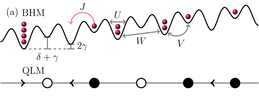
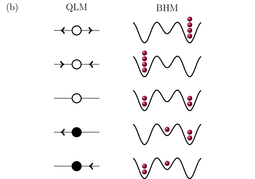
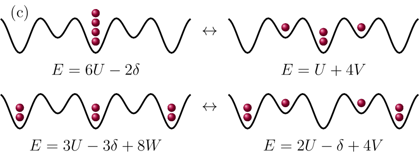
Figure 1: (Color online). (a) The extended Bose–Hubbard model on a tilted optical superlattice with spinless bosons, shown schematically for the case of the spin-$1$ $\mathrm{U}(1)$ QLM (4) as the target theory. The tunneling strength is $J$, on-site interaction strength is $U$, staggering potential is $\delta$, the nearest-neighbor interaction is $V$, the next-nearest-neighbor interaction on the odd sites is $W$, and the tilted potential is $\gamma$. The shallow (deep) sites host matter (gauge) degrees of freedom. The tilted potential $\gamma$ enables the stabilization of the $\mathrm{U}(1)$ gauge invariance. (b) The configurations allowed by Gauss’s law (2) shown in the QLM and BHM representations, where a leftward arrow on a link indicates an electric-field operator eigenvalue of $s^{z}=-1$ (represented by $0$ bosons), a rightward arrow represents $s^{z}=+1$ (represented by $4$ bosons), and an arrowless link denotes $s^{z}=0$ (represented by $2$ bosons). (c) The BHM parameters are determined by enforcing resonances between the shown allowed configurations.

We propose a mapping of the spin-$S$ quantum link model to a superlattice where even (odd) sites represent the matter sites (gauge links) of the gauge theory; see Fig. 1(a). On the even sites, we restrict the local Hilbert subspace to $\mathcal{H}_{\mathrm{m}}=\text{span}\{0,1\}$, while on odd sites to $\mathcal{H}_{\mathrm{g}}=\text{span}\{2n\},\,n\in\{0,1,\ldots,2S\}$. In terms of the electric flux eigenvalues $s^{z}$ on the odd sites, the allowed bosonic occupations $n_{\text{g}}=0,2,\ldots,4S-2,4S$ correspond to $s^{z}=-S,-S+1,\ldots,S-1,S$, respectively, i.e., $n_{\text{g}}=2(s^{z}+S)$; see Fig. 1(b) for the case of $S=1$. This corresponds to the mapping

$$\hat{\sigma}^{+}_{\ell}=\hat{\mathcal{P}}_{\ell}\hat{b}^{\dagger}_{\ell}\hat{\mathcal{P}}_{\ell},\,\,\,\,\,\,\,\hat{\sigma}^{z}_{\ell}=\hat{\mathcal{P}}_{\ell}\big{(}2\hat{b}^{\dagger}_{\ell}\hat{b}_{\ell}-1\big{)}\hat{\mathcal{P}}_{\ell},$$ (3a)

$$\hat{\tau}^{+}_{\ell,\ell+1}=\frac{1}{\sqrt{2S(2S+1)}}\hat{\mathcal{P}}_{\ell,\ell+1}\big{(}\hat{b}^{\dagger}_{\ell,\ell+1}\big{)}^{2}\hat{\mathcal{P}}_{\ell,\ell+1},$$ (3b)

$$\hat{s}^{z}_{\ell,\ell+1}=\frac{1}{4S}\hat{\mathcal{P}}_{\ell,\ell+1}\big{(}\hat{b}^{\dagger}_{\ell,\ell+1}\hat{b}_{\ell,\ell+1}-2S\big{)}\hat{\mathcal{P}}_{\ell,\ell+1},$$ (3c)

where $\hat{b},\hat{b}^{\dagger}$ are local bosonic ladder operators, $\hat{\mathcal{P}}_{\ell}$ and $\hat{\mathcal{P}}_{\ell,\ell+1}$ are projectors onto the local Hilbert subspaces $\mathcal{H}_{\mathrm{m}}$ and $\mathcal{H}_{\mathrm{g}}$, respectively, and in Eq. (3b) we have introduced a “proto” spin-$S$ representation of the gauge field in lieu of the rescaled actual spin-$S$ raising operator $\hat{s}^{+}_{\ell,\ell+1}/\sqrt{S(S+1)}$. Strictly speaking, a QLM is adequate to describe the low-energy subspace of lattice QED. From a particle-physics perspective, this means that the QLM representation is valid only for states $\ket{S,s^{z}}$ with $\lvert s^{z}\rvert\ll S$. As such, in the limit of $S\to\infty$, where the lattice QED limit is achieved, and for finite $s^{z}$, we have $\bra{S,\tilde{s}^{z}}\hat{s}^{+}\ket{S,s^{z}}/\sqrt{S(S+1)}=\delta_{\tilde{s}^{z},s^{z}+1}\sqrt{S(S+1)-\tilde{s}^{z}s^{z}}/\sqrt{S(S+1)}\to 1$. It is in this low-energy limit that one cannot resolve the difference between the infinite-dimensional gauge-field operator of lattice QED and $\hat{s}^{+}/\sqrt{S(S+1)}$. Similarly, in the regime of $S\gg 1$ and a bosonic occupation $n_{\text{g}}\approx 2S-\alpha$ [where $\alpha\ll S$ and is even (odd) for (half-)integer $S$] on the gauge site, we have $\bra{n_{\text{g}}+2}\hat{\tau}^{+}\ket{n_{\text{g}}}\approx 1$, and thus $\hat{\tau}^{+}$ will be indistinguishable from $\hat{s}^{+}/\sqrt{S(S+1)}$, and hence from the gauge-field operator of lattice QED, in the low-energy limit. These considerations are akin to the ones justifying the approximation of lattice QED through highly-occupied bosonic models Zohar and Reznik (2011); Yang et al. (2017). In what follows, we will use $\hat{\tau}^{+}$. A comparison to the dynamics under $\hat{s}^{+}$ is given in Appendix D, showing little qualitative difference between the two representations for relevant physical phenomena.

III Ultracold-atom setup

In the rest of this work, we focus on the case of $S=1$. In this section, we outline an experimentally feasible scheme for mapping the target QLM Hamiltonian

$$\hat{H}_{\text{tar}}= \frac{\kappa}{2}\sum_{\ell=1}^{N-1}\big{(}\hat{\sigma}^{-}_{\ell}\hat{\tau}^{+}_{\ell,\ell+1}\hat{\sigma}^{-}_{\ell+1}+\text{H.c.}\big{)}+\frac{\mu}{2}\sum_{\ell=1}^{N}\hat{\sigma}^{z}_{\ell}$$

$$+\frac{g^{2}}{2}\sum_{\ell=1}^{N-1}\big{(}\hat{s}^{z}_{\ell,\ell+1}\big{)}^{2},$$ (4)

onto the extended Bose–Hubbard model (BHM)

$$\hat{H}_{\text{BHM}}= -J\sum_{j=1}^{L-1}\big{(}\hat{b}_{j}^{\dagger}\hat{b}_{j+1}+\text{H.c.}\big{)}+\frac{U}{2}\sum_{j=1}^{L}\hat{n}_{j}\big{(}\hat{n}_{j}-1\big{)}$$

$$+\sum_{j=1}^{L}\left[(-1)^{j}\frac{\delta}{2}+j\gamma\right]\hat{n}_{j}+V\sum_{j=1}^{L-1}\hat{n}_{j}\hat{n}_{j+1}$$

$$+W\sum_{j=1}^{\frac{L}{2}-1}\hat{n}_{2j-1}\hat{n}_{2j+1}.$$ (5)

Here, $L=2N$ is the total number of bosonic sites $j$ with even (odd) $j$ representing a matter (gauge) site, $\hat{n}_{j}=\hat{b}_{j}^{\dagger}\hat{b}_{j}$ is the bosonic number operator, $U$ is the on-site interaction strength, $\delta$ is a staggered potential making even (odd) sites shallow (deep), and $\gamma$ is a lattice tilt. The microscopic model with target $S>1/2$ has more configurations available than $S=1/2$. To render the physical configurations resonant in the case of $S=1$, this requires a crucial further ingredient, namely interactions beyond on-site given by the nearest-neighbor interaction strength $V$ and the strength of interactions between two consecutive odd sites $W$ (see Fig. 1).

These parameters are not independent, and they should be chosen such that the gauge-invariant processes between configurations allowed by Gauss’s law are resonant; see Fig. 1(c). This leads to two equations with four unknowns:

$$5U-2\delta-4V\approx 0,$$ (6a)

$$U-2\delta-4V+8W\approx 0.$$ (6b)

This underdetermined system of equations allows for a large range of possible values for the parameters, which can be scanned for experimental feasibility.

The parameters of Eqs. (1) and (5) can be connected to each other by relating the processes in Fig. 1(c) in the QLM and BHM pictures and employing perturbation theory (up to second order), which leads to (see Appendix A for derivational details)

$$\mu =-\frac{3}{2}U+\delta+2V-2W+\frac{16J^{2}\big{(}5U-6\delta\big{)}}{\big{(}5U-6\delta\big{)}^{2}-16\gamma^{2}},$$ (7a)

$$g^{2} =4U-8W,$$ (7b)

$$\kappa =\frac{16\sqrt{6}J^{2}\big{(}2\delta-3U\big{)}}{(2\delta-3U\big{)}^{2}-16\gamma^{2}}.$$ (7c)

Ultracold atoms trapped in optical lattices form a convenient quantum simulator for the realization of the target spin-$S$ $\mathrm{U}(1)$ QLM given by Eq. (4). The envisioned system consists of ultracold dipolar bosonic atoms and a $1$D optical superlattice with a relatively small periodicity, described by an extended Bose–Hubbard model where a long-range-type interaction is included Dutta et al. (2015); Baier et al. (2016); Chomaz et al. (2022).

We suggest using a bichromatic superlattice to construct the $1$D trapping potential Fölling et al. (2007); Trotzky et al. (2008). For the 1D linear case, the lattice potential can be written as $V_{s}\cos^{2}(4\pi x/\lambda)-V_{l}\cos^{2}(2\pi x/\lambda-\pi/4)$, where $V_{s,l}$ are the lattice depths of the ‘short’ and the ‘long’ lattice, respectively, and $\lambda$ is the wavelength of the ‘short’ lattice. In such a configuration, the dynamics of the model can be realized by adjusting the lattice depth, thus tuning the tunnelling $J$ and the on-site interaction $U$, as well as the relative depth of the superlattice, thus tuning the energy offset $\delta$ Yang et al. (2020a). The lattice tilt $\gamma$ can be realized by a linear potential acting on the atoms, such as generated by the gravitational force or by a magnetic field acting on the atoms. In addition, the nearest- and next-nearest-neighbor interactions, $V$ and $W$, respectively can be realized by controlling the dipole-dipole interaction between highly magnetic atoms Chomaz et al. (2022); Lahaye et al. (2009); Griesmaier et al. (2005); Lu et al. (2011); Aikawa et al. (2012).

To prepare the initial state with a special ordering, we propose driving the system from a superfluid state to a Mott-insulator regime in an optical superlattice Greiner et al. (2002); Spielman et al. (2007); Bakr et al. (2010); Sherson et al. (2010); Yang et al. (2020b). The overlapping of the intensity minima of the optical lattices creates a large occupation imbalance between neighboring lattice sites, which directs the atoms to occupy the ‘deep’ lattice sites. This allows us to engineer the atom occupation to satisfy Gauss’s law of Eq. (2), resulting in the system being tailored into the gauge-allowed subspace. For instance, we can generate the vacuum state denoted by $\ket{\ldots,2,0,2,0,2,0,\ldots}$. The number fluctuations of this Mott-insulator state can be controlled by lowering the temperature of the system Yang et al. (2020b) or by implementing a state manipulation process Yang et al. (2017); Greif et al. (2013).

A crucial ingredient of the above setup are interactions beyond on-site. To judge the feasibility, we estimate the interaction strengths of bosonic Dysprosium atoms Lu et al. (2011) in the type of optical superlattice proposed above. When the short-lattice laser is set to a wavelength of $\lambda=380\,\text{nm}$, the maximum nearest-neighbor dipole–dipole interaction in the repulsive side is around $V=160\,\text{Hz}$, where we set Planck’s constant to unity. In a linear-type lattice, this interaction between atoms scales with $1/x^{3}$ over distance $x$, and therefore the next-nearest-neighbor interaction in a linear system has a strength of approximately $W=V/2^{3}=20\,\text{Hz}$. Unfortunately, such a relation $V=8W$ leads to unwanted terms appearing in second-order perturbation theory which restrict the dynamics of the gauge theory, as shown in Appendix A.2. These unwanted terms can be removed by setting $V=2W$. However, obtaining such a ratio requires us to shorten the distance between relevant sites. To achieve a controllable distance between the next-nearest-neighbor lattice sites, instead of a linear $1$D lattice, a zigzag ladder can be employed Greschner et al. (2013); Zhang and Jo (2015); Cabedo et al. (2020); Singha Roy et al. (2022); Barbiero et al. (2022). This approach enables us to enhance the interaction strength to approximately $W=80\,\text{Hz}$, thus removing unwanted processes in second-order perturbation theory.

The dipolar interactions between atoms imposes constraints on the other energy scales such as $J$, $U$, $\delta$, and $\gamma$. In the Hubbard regime, the corresponding parameter strengths can be reached by tuning the lattice confinement. Therefore, one can realize the spin-$S$ model in a state-of-the-art extended Bose–Hubbard quantum simulator while suppressing any gauge-violating dynamics.

IV Quench dynamics

We now benchmark our proposed ultracold-atom quantum simulator by probing quench dynamics on it and comparing with the target QLM (4). For this, we employ MPS techniques Schollwöck (2011); Paeckel et al. (2019); McCulloch and perform the time evolution using the time-dependent variational principle (TDVP) Haegeman et al. (2011, 2016). Details of the numerical implementation are provided in Appendix B. Our benchmarking will focus on the spatial averages of electric flux, chiral condensate, and gauge violation,

$$\mathcal{E}(t) =\frac{1}{N-1}\sum_{\ell=1}^{N-1}(-1)^{\ell}\langle\hat{s}^{z}_{\ell,\ell+1}(t)\rangle,$$ (8a)

$$\mathcal{C}(t) =\frac{1}{2}+\frac{1}{2N}\sum_{\ell=1}^{N}\langle\hat{\sigma}^{z}_{\ell}(t)\rangle,$$ (8b)

$$\eta(t) =\sqrt{\frac{1}{N}\sum_{\ell=1}^{N}\langle\hat{G}_{\ell}^{2}(t)\rangle},$$ (8c)

respectively. We seek very good quantitative agreement in the quench dynamics of the electric flux and chiral condensate between the BHM and QLM, which should correspond to a very small and controlled gauge violation over the entire time evolution.

Throughout this section, we set our parameters to $J=3$ Hz, $\gamma=7$ Hz, $V=160$ Hz, and $W=80$ Hz, which are experimentally feasible values in the zigzag scheme discussed in Sec. III. Benchmarks of the linear architecture are included in Appendix C.

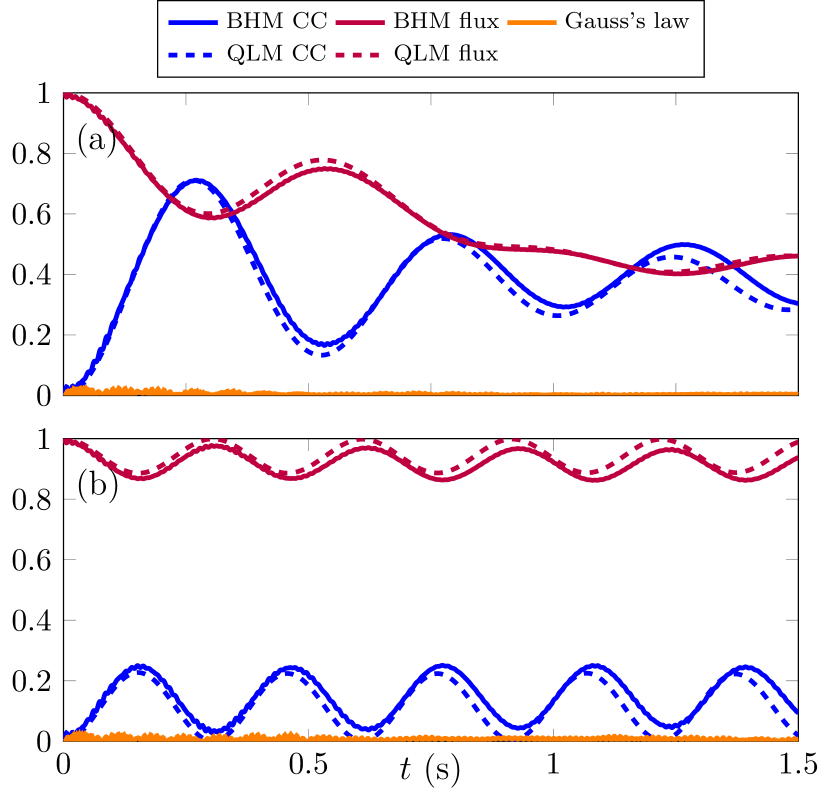
Figure 2: (Color online). Numerical simulations of a global quench of the extreme vacuum state in the BHM (5) (solid lines) and target QLM (4) (dashed). The values of the electric flux (8a) and chiral condensate (8b) show good agreement, and the gauge violation in the BHM (8c) remains on low levels throughout the entire time evolution. (a) Quench to $U=160$ Hz and $\delta=80$ Hz, which corresponds to $\mu/\kappa\approx-0.41$ and $g^{2}/\kappa=0$ in the target model. (b) Quench to $U=159$ Hz and $\delta=78.5$ Hz, which corresponds to $\mu/\kappa\approx-0.40$ and $g^{2}/\kappa\approx 3.60$ in the target model.

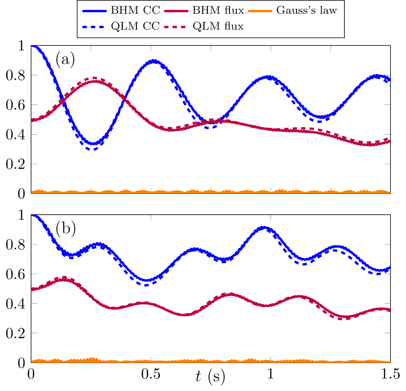
Figure 3: (Color online). Numerical simulations of a global quench of the charge-proliferated state in the BHM (5) and target QLM (4). Again, the values of the electric flux (8a) and chiral condensate (8b) show good agreement, and the gauge violation in the BHM (8c) remains small. The quench parameters for each panel are the same as in the corresponding panels of Fig. 2.

We are interested in gauge-invariant translation-invariant states in the QLM that can be represented by an infinitely repeating unit cell of two matter sites and two gauge links $\lvert\sigma^{z}_{\ell},s^{z}_{\ell,\ell+1},\sigma^{z}_{\ell+1},s^{z}_{\ell+1,\ell+2}\rangle$, where $\sigma^{z}_{\ell}$ and $s^{z}_{\ell,\ell+1}$ are the eigenvalues of $\hat{\sigma}^{z}_{\ell}$ and $\hat{s}^{z}_{\ell,\ell+1}$, respectively. In the bosonic mapping, this state is represented as $\ket{n_{j},n_{j+1},n_{j+2},n_{j+3}}$, where $n_{j}$ is the eigenvalue of $\hat{n}_{j}$ of the optical superlattice, and $j$ is an even site representing a matter site in the QLM, and odd bosonic sites in the BHM represent gauge links in the QLM. We emphasize that our MPS calculations work directly in the thermodynamic limit for these states, and they are infinite in spatial extent (see Appendix B).

In particular, we consider the following three types of initial states (“vacua”). The “highly excited” or “extreme vacua” of the QLM, given by $\ket{-1,\pm 1,-1,\mp 1}$ (bosonic mapping: $\ket{0,4,0,0}$ and $\ket{0,0,0,4}$, respectively), corresponding to absence of charges and maximal allowed values of electric field (for $S=1$); the “middle vacuum” $\ket{-1,0,-1,0}$ (bosonic mapping: $\ket{0,2,0,2}$), corresponding to absence of charged particles and vanishing electric field; and the charge-proliferated states $\ket{+1,0,+1,-1}$ and $\ket{+1,-1,+1,0}$ (bosonic mapping: $\ket{1,2,1,0}$ and $\ket{1,0,1,2}$), corresponding to presence of charges with electric fields between neighboring pairs of particles; see Fig. 1(b) for the mapping between the QLM and BHM pictures.

IV.1 Extreme vacuum

To begin with, we consider the extreme vacuum state $\ket{-1,1,-1,-1}$, which in the bosonic picture is $\ket{0,4,0,0}$. We first consider a quench at $U=160$ Hz and $\delta=80$ Hz, which corresponds to $\mu/\kappa\approx-0.41$ and $g^{2}/\kappa=0$ in the target QLM. The corresponding quench dynamics of the electric flux, chiral condensate, and gauge violation are shown in Fig. 2(a), with solid (dashed) lines corresponding to the BHM (QLM). We see very good quantitative agreement in the quench dynamics of the electric flux and chiral condensate between the BHM and QLM, which is a testament to the faithfulness of our proposed quantum simulator. Indeed, the gauge violation over the whole duration of the dynamics, roughly $1.5$ seconds, is very well suppressed and never exceeds $3\%$.

As a second benchmark case, we quench the extreme vacuum to the model parameters $U=159$ Hz and $\delta=78.5$ Hz, which corresponds to $\mu/\kappa\approx-0.40$ and $g^{2}/\kappa\approx 3.60$. The corresponding quench dynamics is shown in Fig. 2(b). Again, we find very good quantitative agreement in the dynamics of the electric flux and chiral condensate between the BHM and QLM, and the gauge violation is very well suppressed over all accessible evolution times.

From a phenomenological point of view, we see that the dynamics at the larger value of $g^{2}/\kappa$ is significantly constrained. We will investigate this behavior in more detail below by probing the fate of an electron–positron pair depending on the strength of the gauge coupling.

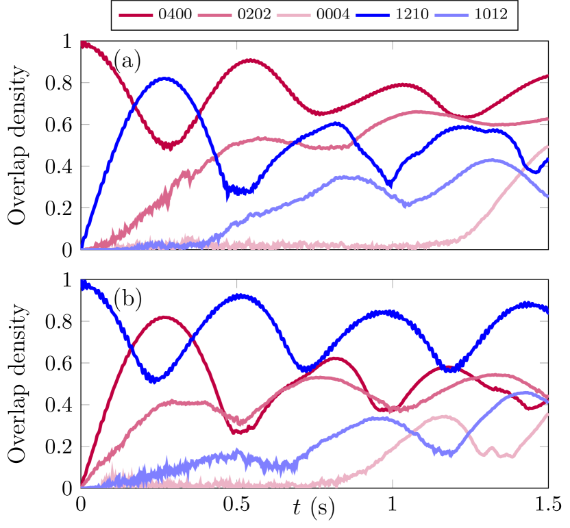
Figure 4: (Color online). Plot of the overlap density (per four site unit cell) of the time evolved states of the global quenches in the BHM with the three vacuum states (shown in shades of red) and two charge-proliferated states (in shades of blue). The time evolution results shown correspond to Fig. 2(a) in panel (a) and Fig. 3(a) in panel (b).

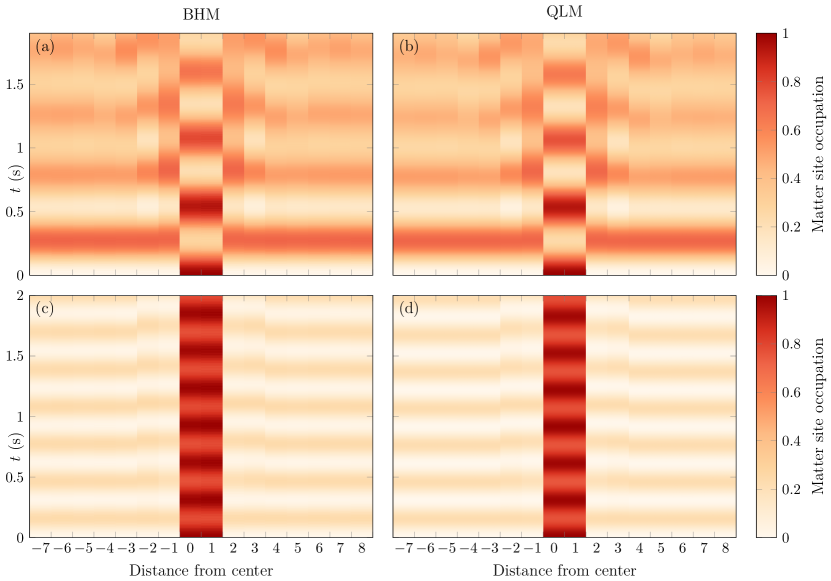
Figure 5: (Color online). Numerical simulations of an electron–positron pair on top of the extreme vacuum in the BHM (5) (panels (a) and (c)) and the target QLM (4) (panels (b) and (d)). (a,b) Quench to $U=160$ Hz and $\delta=80$ Hz, which correspond to $\mu/\kappa\approx-0.41$ and $g^{2}/\kappa=0$ in the target model. (c,d) Quench to $U=159$ Hz and $\delta=78.5$ Hz, which correspond to $\mu/\kappa\approx-0.40$ and $g^{2}/\kappa\approx 3.60$ in the target model.

IV.2 Charge-proliferated state

Next, we consider as initial state the charge-proliferated state $\ket{+1,0,+1,-1}$, which in the bosonic picture is $\ket{1,2,1,0}$. We repeat the same quenches employed in Sec. IV.1 for the extreme vacuum, and the corresponding quench dynamics are presented in Fig. 3. In both cases, we again see very robust quantitative agreement in the quench dynamics of the electric flux and chiral condensate between the BHM and QLM up to all investigated evolution times. The proposed BHM quantum simulator further demonstrates its faithfulness by exhibiting a very suppressed gauge violation throughout the entire dynamics.

It is interesting to calculate the overlap of the time-evolved wave function with the three vacua and two charge-proliferated states of the target QLM for quenches considered in Secs. IV.1 and IV.2. We show this in Fig. 4(a,b) for the quenches of Figs. 2(a) and 3(a), respectively. The quench dynamics shows significant overlap of the wave function with all these five product states, signifying the system indeed takes full advantage of the additional configurations available thanks to the effective spin-$1$ representation of the gauge and electric fields.

IV.3 Electron–positron pair and confinement

Confinement is one of the most intriguing phenomena of gauge theories, and there have been several proposals to probe confinement in quantum simulators of gauge theories for spin-$1/2$ $\mathrm{U}(1)$ QLMs involving the implementation of a topological $\theta$-angle Surace et al. (2020); Halimeh et al. (2022b); Cheng et al. (2022). Whereas in the latter the gauge-coupling term $(g^{2}/2)\sum_{\ell}(\hat{s}^{z}_{\ell,\ell+1})^{2}$ is an inconsequential energy constant since $(\hat{s}^{z}_{\ell,\ell+1})^{2}=\mathds{1}/4$ for $S=1/2$, this term is dynamic in the case of $S=1$, and is known to cause confinement at strong gauge coupling (i.e., when $g$ is large) Chandrasekharan (1999). QLMs with integer values of $S$ resemble the Wilson-Kogut-Susskind formulation of $\mathrm{U}(1)$ lattice gauge theories Kogut and Susskind (1975), in which confinement in the strong-coupling regime has been studied Byrnes et al. (2002). The gauge-coupling term becomes equivalent to an energetic constraint that penalizes large deviations from the original configuration of flux strings. Indeed, at large values of $\lvert g^{2}/\kappa\rvert\gg 1$, the gauge-coupling term can be thought of as inducing coherent quantum Zeno dynamics Facchi and Pascazio (2002); Facchi et al. (2004, 2009); Burgarth et al. (2019) that constrains the time evolution in a small subspace of the total Gauss’s law sector.

In order to properly probe (de)confinement in our target QLM, we turn to a paradigmatic test state and prepare an electron–positron pair on top of the extreme vacuum considered in Sec. IV.1. This state breaks translation invariance, and as such we cannot employ infinite MPS, but rather we restrict ourselves to a finite system of $N=40$ matter sites (see Appendix B).

Quenching this pair state with the BHM model at $U=2\delta=160$ Hz, which corresponds to $\mu/\kappa\approx-0.41$ and $g^{2}/\kappa=0$ in the target QLM, we find a rapid spread of the pair indicating deconfinement, as shown in the matter density profile in Fig. 5(a,b) for the BHM and target QLM, respectively. Note how the quantitative agreement in the dynamics between both models is excellent over all investigated evolution times. The gauge violation in the BHM simulations is well suppressed and never exceeds $3\%$, as with the quenches of the translation-invariant states.

We now probe the dynamics of the electron–positron pair at a large value of the gauge coupling $g$. We quench the pair state with the BHM model at $U=159$ Hz and $\delta=78.5$ Hz, which corresponds to $\mu/\kappa\approx-0.40$ and $g^{2}/\kappa\approx 3.60$ in the target QLM. The resulting quench dynamics, shown in Fig. 5(c,d) for the BHM and QLM, respectively, shows fundamentally different behavior from the case of $g^{2}=0$. Indeed, the electron–positron pair appears to be bound and immobile for all accessible evolution times in MPS, which is a clear signature of confinement. Also in this case, the quantitative agreement in the quench dynamics between the BHM and QLM is excellent, with the gauge violation in the BHM simulation being well controlled.

Furthermore, this is the (de)confinement behavior expected in the “ideal” spin-$1$ $\mathrm{U}(1)$ QLM (1) Chandrasekharan (1999), and, indeed, the corresponding dynamics for the same quench in the latter is qualitatively similar to that of Fig. 5, as shown in Fig. 8 in Appendix D.

V Linear gauge protection

It would be instructive to get a better understanding of the excellent suppression of gauge violations that we find over all investigated evolution times in our quench dynamics. As already mentioned, the tunneling term in Hamiltonian (5) is the perturbation that breaks gauge invariance, although it induces effective gauge-theory dynamics due to a large energetic penalty on processes driving the dynamics away from the physical sector. To illustrate this, let us consider the part of Hamiltonian (5) that is diagonal in the particle-number basis, and write it using QLM spatial indexing,

$$\hat{H}_{\text{diag}}=\sum_{\ell}\bigg{\{} \frac{U}{2}\Big{[}\hat{n}_{\ell}\big{(}\hat{n}_{\ell}-1\big{)}+\hat{n}_{\ell,\ell+1}\big{(}\hat{n}_{\ell,\ell+1}-1\big{)}\Big{]}$$

$$-\delta\hat{n}_{\ell,\ell+1}+2(-1)^{\ell}\ell\gamma\hat{G}_{\ell}+W\hat{n}_{\ell-1,\ell}\hat{n}_{\ell,\ell+1}$$

$$+V\big{[}\hat{n}_{\ell-1,\ell}\hat{n}_{\ell}+\hat{n}_{\ell}\hat{n}_{\ell,\ell+1}\big{]}\bigg{\}},$$ (9)

up to an inconsequential energetic constant, where we have rewritten the generator (2) of Gauss’s law in the bosonic basis as

$$\hat{G}_{\ell}=(-1)^{\ell}\bigg{(}\hat{n}_{\ell}+\frac{\hat{n}_{\ell-1,\ell}+\hat{n}_{\ell,\ell+1}}{2}-2S\bigg{)}.$$ (10)

We can identify in Eq. (9) a linear gauge protection term $\hat{H}_{G}=\sum_{\ell}2(-1)^{\ell}\ell\gamma\hat{G}_{\ell}$, which has been shown to stabilize gauge invariance up to all numerically accessible evolution times Halimeh et al. (2021); Lang et al. (2022). This explains the excellent stabilization of gauge invariance in all of our results. The other diagonal terms in the BHM are needed to ensure that the accessible states in perturbation theory correspond to physical states in the QLM, as detailed in Appendix A.

VI Conclusion and outlook

We have presented a general mapping of spin-$S$ $\mathrm{U}(1)$ quantum link models onto bosonic ultracold atoms on an optical superlattice. In keeping with experimental feasibility on current ultracold-atom quantum technologies, we have proposed an extended single-species Bose–Hubbard quantum simulator of a spin-$1$ $\mathrm{U}(1)$ quantum link model. Using perturbation theory, we have derived the exact relations between the parameters of the quantum simulator and the quantum link model.

Using matrix product state techniques and the time-dependent variation principle, we benchmarked the quench dynamics of local observables in the quantum link model with that of the quantum simulator, showing great quantitative agreement up to all accessible evolution times. In all cases, the gauge violation was strongly suppressed and controlled over all investigated evolution times. We showed how this was a result of a linear gauge protection term naturally arising in our mapping.

We demonstrated the ability of our quantum simulator to probe relevant high-energy phenomena by calculating the quench dynamics of an electron–positron pair, showing a confinement–deconfinement transition by tuning the gauge coupling $g$.

Our work opens the door towards larger-spin representations of quantum link model regularizations of quantum electrodynamics on modern quantum-simulator platforms, and is amenable to several extensions. For example, a topological $\theta$-term can be implemented by adding an additional staggering to the gauge sites in the optical superlattice Halimeh et al. (2022b); Cheng et al. (2022). Furthermore, it is possible to extend our setup to $2+1$D along the lines of recent proposals Osborne et al. (2022); Surace et al. (2023).

Appendix A Perturbation theory

To determine the values of the tunneling strength $\kappa$ and the diagonal terms ($\mu$ and $g$) in the target QLM for our BHM setup, we only need to consider translation-invariant states with a four-site unit cell in the BHM (which corresponds to two matter sites and two gauge links in the QLM mapping). This is sufficient to describe all possible homogeneous gauge-invariant states and the processes that couple them. Since our BHM setup has interaction terms that affect inhomogeneous states nontrivially, we will examine the effect this has on the target QLM Hamiltonian afterwards.

A.1 Homogeneous states

Let us consider the possible states for a translation-invariant unit cell of four sites in the BHM, which corresponds to two matter sites in the QLM mapping. We have a total of four bosons per four-site unit cell. We only consider the states corresponding to gauge-invariant states in the QLM mapping and states which can be obtained from these states by hopping a single boson (for brevity, we will only consider one of the two extreme vacua and charge-proliferated states, since the other ones do not provide any additional information). We label these states as $\ket{i}$ for $i=1,\ldots,11$: their boson configurations (where the first site in the unit cell corresponds to a matter site) and energy densities are

$$\ket{1} =\ket{0400}, E_{1} =6U-2\delta,$$ (11a)

$$\ket{2} =\ket{1300}, E_{2} =3U-\delta+3V-\gamma,$$ (11b)

$$\ket{3} =\ket{0310}, E_{3} =3U-\delta+3V+\gamma,$$ (11c)

$$\ket{4} =\ket{1210}, E_{4} =U+4V,$$ (11d)

$$\ket{5} =\ket{2110}, E_{5} =U+\delta+3V-\gamma,$$ (11e)

$$\ket{6} =\ket{1120}, E_{6} =U+\delta+3V+\gamma,$$ (11f)

$$\ket{7} =\ket{0211}, E_{7} =U-\delta+3V+4W-\gamma,$$ (11g)

$$\ket{8} =\ket{1201}, E_{8} =U-\delta+3V+4W+\gamma,$$ (11h)

$$\ket{9} =\ket{0202}, E_{9} =2U-2\delta+8W,$$ (11i)

$$\ket{10} =\ket{1102}, E_{10} =E_{7},$$ (11j)

$$\ket{11} =\ket{0112}, E_{11} =E_{8}.$$ (11k)

The nonzero off-diagonal elements of the Hamiltonian $\hat{H}=\hat{H}_{\text{BHM}}$ are

$$\matrixelement{1}{\hat{H}}{2}=\matrixelement{1}{\hat{H}}{3} =-2J,$$ (12a)

$$\matrixelement{2}{\hat{H}}{4}=\matrixelement{3}{\hat{H}}{4} =-\sqrt{3}J,$$ (12b)

$$\matrixelement{4}{\hat{H}}{5}=\matrixelement{4}{\hat{H}}{6} =-2J,$$ (12c)

$$\matrixelement{4}{\hat{H}}{7}=\matrixelement{4}{\hat{H}}{8} =-J,$$ (12d)

$$\matrixelement{i}{\hat{H}}{9} =-\sqrt{2}J,\qquad i=7,8,10,11,$$ (12e)

and their conjugate elements, which are the same (e.g., $\matrixelement{2}{\hat{H}}{1}=\matrixelement{1}{\hat{H}}{2}$).

We now employ a Schrieffer–Wolff transformation on the Hamiltonian, which we rewrite in the form

$$\hat{H}=\hat{H}_{0}+\hat{H}_{1},$$ (13)

where $\hat{H}_{0}$ contains all of the diagonal elements and $\hat{H}_{1}$ contains all of the off-diagonal elements. We then wish to find the transformed effective Hamiltonian

$$\hat{H}_{\text{eff}}=\mathrm{e}^{\mathrm{i}\hat{S}}\hat{H}\mathrm{e}^{-\mathrm{i}\hat{S}},$$ (14)

where $\hat{S}$ is a small-valued Hermitian matrix that we need to find. By the Baker–Campbell–Hausdorff formula, we have that

$$\hat{H}_{\text{eff}} =\hat{H}+\mathrm{i}[\hat{S},\hat{H}]-\frac{1}{2}[\hat{S},[\hat{S},\hat{H}]]+\mathcal{O}(\hat{S}^{3}).$$ (15)

We neglect the terms $\mathcal{O}(\hat{S}^{3})$, and define $\hat{S}$ such that

$$[\hat{S},\hat{H}_{0}]=\mathrm{i}\hat{H}_{1},$$ (16)

which allows us to obtain

$$\hat{H}_{\text{eff}}\approx\hat{H}_{0}+\frac{1}{2}\mathrm{i}[\hat{S},\hat{H}_{1}].$$ (17)

We can find the matrix elements of $\hat{S}$ in the basis $\{\ket{i}\}_{i=1,\ldots,9}$ by using our definition of $\hat{S}$ (16) and using the fact that $\hat{H}_{0}$ is diagonal

$$\matrixelement{i}{\hat{S}}{j}=\mathrm{i}\frac{\matrixelement{i}{\hat{H}_{1}}{j}}{E_{j}-E_{i}},$$ (18)

where $E_{i}\equiv\matrixelement{i}{\hat{H}_{0}}{i}$. The matrix elements of the effective Hamiltonian (17) in the basis $\{\ket{i}\}_{i=1,\ldots,9}$ are thus

$$\matrixelement{i}{\hat{H}_{\text{eff}}}{j}=\delta_{ij}E_{i}\\ +\frac{1}{2}\sum_{k}\left(\frac{1}{E_{i}-E_{k}}+\frac{1}{E_{j}-E_{k}}\right)\matrixelement{i}{\hat{H}_{1}}{k}\matrixelement{k}{\hat{H}_{1}}{j}.$$ (19)

Note that our assumption that $\hat{S}$ was small-valued in order to neglect terms $\mathcal{O}(\hat{S}^{3})$ implies that we need $\lvert\matrixelement{i}{\hat{H}_{1}}{j}\rvert\ll\lvert E_{j}-E_{i}\rvert$ by Eq. (18). That is, we require the energies of the gauge-invariant states $\{\ket{1},\ket{4},\ket{9}\}$ to be well-separated from the energies of the other states to which they are coupled by $\hat{H}_{1}$. This condition is generally satisfied, although care needs to be taken particularly with the choice of $\gamma$ to make sure such resonances do not occur. In this regime, we can truncate the basis of the effective Hamiltonian to the gauge-invariant states, and calculate their matrix elements as follows (where the labels above each term show which state is responsible for it, and the notation $(\gamma\rightarrow-\gamma)$ is an abbreviation for the previous terms but with $\gamma$ replaced with $-\gamma$):

$$\matrixelement{1}{\hat{H}_{\text{eff}}}{1} =6U-2\delta+4J^{2}\bigg{[}\overbrace{\frac{1}{3U-\delta-3V+\gamma}}^{\text{via}~{}\ket{2}}+\overbrace{(\gamma\rightarrow-\gamma)}^{\text{via}~{}\ket{3}}\bigg{]},$$ (20a)

$$\matrixelement{1}{\hat{H}_{\text{eff}}}{4} =\sqrt{3}J^{2}\bigg{[}\overbrace{\frac{1}{3U-\delta-3V+\gamma}+\frac{1}{-2U+\delta+V+\gamma}}^{\text{via}~{}\ket{2}}+\overbrace{(\gamma\rightarrow-\gamma)}^{\text{via}~{}\ket{3}}\bigg{]},$$ (20b)

$$\matrixelement{4}{\hat{H}_{\text{eff}}}{4} =U+4V+J^{2}\bigg{[}\overbrace{\frac{3}{-2U+\delta+V+\gamma}}^{\text{via}~{}\ket{2}}+\overbrace{\frac{1}{\delta+V-4W+\gamma}}^{\text{via}~{}\ket{7}}+\overbrace{\frac{4}{-\delta+V+\gamma}}^{\text{via}~{}\ket{5}}+\overbrace{(\gamma\rightarrow-\gamma)}^{\text{via}~{}\ket{3},\ket{6},\ket{8}}\bigg{]},$$ (20c)

$$\matrixelement{4}{\hat{H}_{\text{eff}}}{9} =\frac{\sqrt{2}J^{2}}{2}\bigg{[}\overbrace{\frac{1}{\delta+V-4W+\gamma}+\frac{1}{U-\delta-3V+4W+\gamma}}^{\text{via}~{}\ket{7}}+\overbrace{(\gamma\rightarrow-\gamma)}^{\text{via}~{}\ket{8}}\bigg{]},$$ (20d)

$$\matrixelement{9}{\hat{H}_{\text{eff}}}{9} =2U-2\delta+8W+4J^{2}\bigg{[}\overbrace{\frac{1}{U-\delta-3V+4W+\gamma}}^{\text{via}~{}\ket{7},\ket{10}}+\overbrace{(\gamma\rightarrow-\gamma)}^{\text{via}~{}\ket{8},\ket{11}}\bigg{]}.$$ (20e)

Close to resonance (6), we have that

$$V \approx\frac{5U}{4}-\frac{\delta}{2},$$ (21a)

$$4W \approx-\frac{U}{2}+\delta+2V\approx 2U.$$ (21b)

By using these conditions, we can obtain simplified expressions for the parameters in the target QLM as

$$g^{2} =\matrixelement{1}{\hat{H}_{\text{eff}}}{1}-\matrixelement{9}{\hat{H}_{\text{eff}}}{9}=4U-8W,$$ (22a)

$$\mu =\frac{1}{2}\left[\matrixelement{4}{\hat{H}_{\text{eff}}}{4}-\matrixelement{9}{\hat{H}_{\text{eff}}}{9}-\frac{g^{2}}{2}\right]$$

$$=-\frac{3}{2}U+\delta+2V-2W$$

$$\quad+2J^{2}\left[\frac{1}{5U/4-3\delta/2+\gamma}+(\gamma\rightarrow-\gamma)\right],$$ (22b)

$$\kappa =\frac{2\sqrt{6}}{2\sqrt{3}}\matrixelement{1}{\hat{H}_{\text{eff}}}{4}=\frac{2\sqrt{6}}{\sqrt{2}}\matrixelement{4}{\hat{H}_{\text{eff}}}{9}$$

$$=2\sqrt{6}J^{2}\left[\frac{1}{-3U/4+\delta/2+\gamma}+(\gamma\rightarrow-\gamma)\right].$$ (22c)

A.2 Inhomogeneous states

In the previous section, we only dealt with homogeneous gauge-invariant states where the matter sites were either all occupied or all unoccupied. Since our BHM setup has first- and second-neighbor interaction terms, the renormalized energies of inhomogeneous configurations will differ from the sum of energies obtained from each individual site using the terms in the previous section.

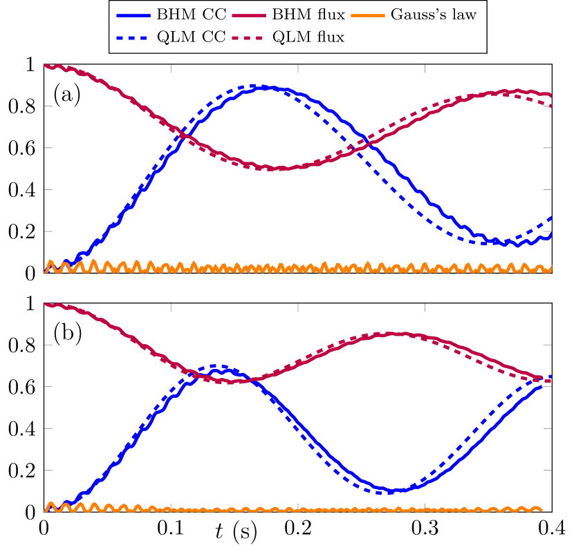
Figure 6: (Color online). Numerical simulations of a global quench of the extreme vacuum state in the BHM (5) and target QLM (4), showing the values of the electric flux (8a) and chiral condensate (8b), as well as the gauge violation in the BHM (8c). These quenches are in a different parameter regime than Fig. 2, which correspond to a linear architecture where extra renormalization terms (25) appear in the Hamiltonian in second-order perturbation theory. Both panels use $J=5$ Hz, $\gamma=57$ Hz, $\delta=-220$ Hz, $V=160$ Hz and $W=20$ Hz. (a) Quench to $U=40$ Hz, which corresponds to $\mu/\kappa\approx-0.13$ and $g^{2}/\kappa=0$ in the target model. (b) Quench to $U=40.5$ Hz, which corresponds to $\mu/\kappa\approx 0.23$ and $g^{2}/\kappa\approx-0.96$ in the target model.

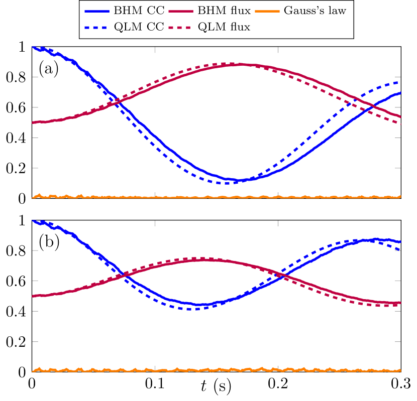
Figure 7: (Color online). Numerical simulations of a global quench of the charge-proliferated state in the BHM (5) and target QLM (4), showing the values of the electric flux (8a) and chiral condensate (8b), as well as the gauge violation in the BHM (8c). The quench parameters for each panel are the same as in Fig. 6.

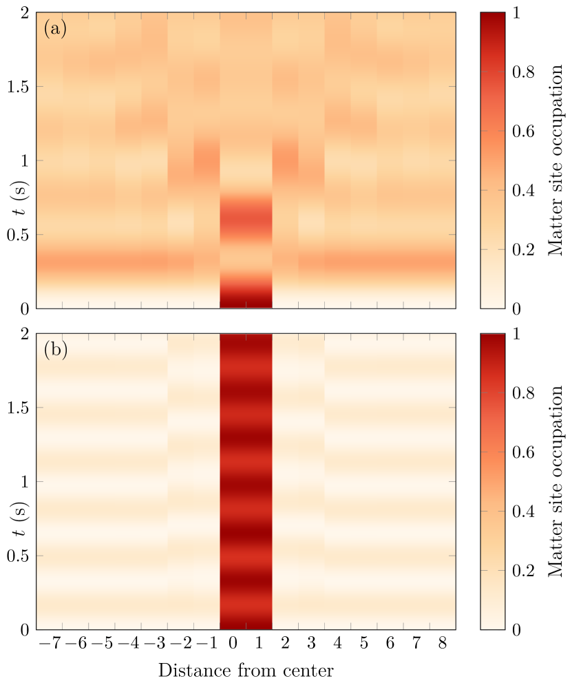
Figure 8: (Color online). Numerical simulations of an electron–positron pair on top of the extreme vacuum in the ideal QLM (4), described by link operators $\hat{s}^{+}_{\ell,\ell+1}/\sqrt{2}$ instead of the $\hat{\tau}^{+}_{\ell,\ell+1}$ used in the main text. The same sets of parameters are used as in Fig. 5. The qualitative difference is very small.

The four relevant configurations (where the first site corresponds to a gauge site) are $\ket{21004}$, $\ket{40012}$, $\ket{01202}$ and $\ket{20210}$. The total energy of each of these configurations is the same as that obtained from the values of $g^{2}$ (22a) and $\mu$ (22b) without the renormalization effects from second-order perturbation theory (i.e., the terms proportional to $J^{2}$). The renormalization for the corresponding terms in the QLM will be different: for the state $\ket{21004}$ the difference in the renormalized energy from that obtained from the homogeneous configurations is

$$E^{21004}=J^{2}\bigg{[}\overbrace{\frac{1}{\delta+2V-6W-\gamma}}^{\ket{21004}\leftrightarrow\ket{20104}}-\overbrace{\frac{1}{\delta+V-4W-\gamma}}^{\ket{21012}\leftrightarrow\ket{20112}}\bigg{]};$$ (23)

the difference for $\ket{40012}$ is the same but with $-\gamma$ replaced with $\gamma$. The difference in the renormalized energy for $\ket{01202}$ is then (with $\ket{20210}$’s difference being obtained similarly by replacing $\gamma$ with $-\gamma$)

$$E^{01202}=J^{2}\bigg{[}\overbrace{\frac{4}{-\delta+2W+\gamma}}^{\ket{01202}\leftrightarrow\ket{02102}}-\overbrace{\frac{4}{-\delta+V+\gamma}}^{\ket{01210}\leftrightarrow\ket{02110}}$$

$$\quad+\overbrace{\frac{3}{-2U+\delta+2V-2W-\gamma}}^{\ket{01202}\leftrightarrow\ket{00302}}-\overbrace{\frac{3}{-2U+\delta+V-\gamma}}^{\ket{01210}\leftrightarrow\ket{00310}}$$

$$\quad+\overbrace{\frac{2}{U-\delta-2V+2W-\gamma}}^{\ket{01202}\leftrightarrow\ket{01112}}-\overbrace{\frac{2}{U-\delta-3V+4W-\gamma}}^{\ket{20202}\leftrightarrow\ket{20112}}\bigg{]}.$$ (24)

To account for these energy shifts in the QLM mapping, we add four extra terms to the QLM Hamiltonian which shift the energy for each of these inhomogeneous configurations

$$H_{\text{inhomog}}=E^{21004}\sum_{\ell}\frac{1+\hat{\sigma}^{z}_{\ell}}{2}\frac{1-\hat{\sigma}^{z}_{\ell+1}}{2}(\hat{s}^{z}_{\ell,\ell+1})^{2}$$

$$\quad+E^{40012}\sum_{\ell}\frac{1-\hat{\sigma}^{z}_{\ell}}{2}\frac{1+\hat{\sigma}^{z}_{\ell+1}}{2}(\hat{s}^{z}_{\ell,\ell+1})^{2}$$

$$\quad+E^{01202}\sum_{\ell}\frac{1+\hat{\sigma}^{z}_{\ell}}{2}\frac{1-\hat{\sigma}^{z}_{\ell+1}}{2}\left[1-(\hat{s}^{z}_{\ell,\ell+1})^{2}\right]$$

$$\quad+E^{20210}\sum_{\ell}\frac{1-\hat{\sigma}^{z}_{\ell}}{2}\frac{1+\hat{\sigma}^{z}_{\ell+1}}{2}\left[1-(\hat{s}^{z}_{\ell,\ell+1})^{2}\right].$$ (25)

Unfortunately, the terms in $H_{\text{inhomog}}$ can severely limit the range of dynamics in the QLM. However, by inspecting the expressions for the energy shifts in Eqs. (23) and (A.2), we can see that each term comes in a pair with a difference of $V-2W$ in the denominators. By setting $V=2W$, the two terms in each pair will cancel each other out, removing the second-order energy shifts of these configurations, and thus retrieving a QLM mapping without the restrictive terms in $H_{\text{inhomog}}$ (25). To obtain $V=2W$ in an experimental setup, we propose using a zigzag architecture, as discussed in Sec. III.

Appendix B Numerical details

We use matrix product state (MPS) techniques Schollwöck (2011); Paeckel et al. (2019); McCulloch to simulate the quench dynamics of the uniform states and electron–positron pair states. The time evolved states are obtained using the time-dependent variational principle (TDVP) algorithm Haegeman et al. (2011, 2016): we use a single-site evolution scheme with adaptive bond dimension growth (Zauner-Stauber et al., 2018, App. B), and use a time-step of $0.1$ ms. For the simulation of the inhomogeneous states containing an electron–positron pair on top of a vacuum, we used a finite system with a width of at least $40$ matter sites, so that any boundary effects would not be visible in the evolution times considered. For the simulation of the uniform initial states, we write the state as an infinite MPS with a translation-invariant four-site unit cell, allowing us to simulate the dynamics directly in the thermodynamic limit.

In order to represent the linear tilt term $\sum_{j}j\gamma\hat{n}_{j}$ in the BHM acting on a translation-invariant state, we perform a transformation to the “dynamic gauge” Zisling et al. (2022), where the tilt term is removed and replaced by a time-dependent phase in the hopping term $\sum_{j}(\mathrm{e}^{\mathrm{i}\gamma t}\hat{b}_{j}^{\dagger}\hat{b}_{j+1}+\text{H.c.})$. This makes the extended BHM amenable to be simulated using infinite MPS techniques, while leaving the expectation values of boson occupation numbers unchanged.

Appendix C Linear architecture

In the main text, we have focused on the zigzag architecture outlined in Sec. III. We can also utilize the linear architecture, also described in Sec. III, but then we are restricted to $W=V/2^{3}$. This leads to the renormalization terms described in Appendix A.2, which modify the form of the target QLM. We shall set $J=5$ Hz, $\gamma=57$ Hz, $V=8W=160$ Hz, and $\delta=-220$ Hz for this architecture.

We now benchmark the BHM quantum simulator based on the linear architecture by quenching the extreme vacuum, already used in Sec. IV.1 and IV.2, but with the BHM at $U=40$ ($40.5$) Hz, which corresponds to a quench by the target QLM with the renormalization term (25) at $\mu/\kappa\approx-0.13$ ($0.23$) and $g^{2}/\kappa\approx 0$ ($-0.96)$. The corresponding quench dynamics of the electric flux and chiral condensate are shown in Fig. 6(a,b) for both sets of parameters, respectively. In both quenches, we find very good quantitative agreement in the dynamics of both observables between the BHM and QLM, with a very suppressed and well-controlled gauge violation over all investigated times.

For completeness, we repeat the same quench protocols but starting in the charge-proliferated state considered in Sec. IV.2, with the corresponding quench dynamics shown in Fig. 7(a,b), respectively. The conclusion is the same as that of Fig. 6 in that the BHM and QLM simulations show very good quantitative agreement in the electric flux and chiral condensate. The gauge violation in the BHM simulation is quite small and well-controlled over all accessible evolution times.

Appendix D Comparison to ideal QLM

As discussed in the main text, the gauge field $\hat{\tau}^{+}_{\ell,\ell+1}$ in the target QLM (4) differs from $\hat{s}^{+}_{\ell,\ell+1}$ of the ideal QLM (1). This can lead to quantitative differences in certain regimes, but it is interesting to check the qualitative effect this different representation will have on a relevant high-energy phenomenon like the (de)confinement of the electron–positron pair studied in Fig. 5 in the main text. To this effect, we repeat the quenches of the target QLM in Fig. 5 but with the ideal QLM Hamiltonian (1). The corresponding result, presented in Fig. 8, shows little qualitative difference in the (de)confinement of the electron–positron pair between quenching with the ideal or target QLM.

References

- Bañuls et al. (2020) Mari Carmen Bañuls, Rainer Blatt, Jacopo Catani, Alessio Celi, Juan Ignacio Cirac, Marcello Dalmonte, Leonardo Fallani, Karl Jansen, Maciej Lewenstein, Simone Montangero, Christine A. Muschik, Benni Reznik, Enrique Rico, Luca Tagliacozzo, Karel Van Acoleyen, Frank Verstraete, Uwe-Jens Wiese, Matthew Wingate, Jakub Zakrzewski, and Peter Zoller, “Simulating lattice gauge theories within quantum technologies,” The European Physical Journal D 74, 165 (2020).
- Dalmonte and Montangero (2016) M. Dalmonte and S. Montangero, “Lattice gauge theory simulations in the quantum information era,” Contemporary Physics 57, 388–412 (2016).
- Zohar et al. (2015) Erez Zohar, J Ignacio Cirac, and Benni Reznik, “Quantum simulations of lattice gauge theories using ultracold atoms in optical lattices,” Reports on Progress in Physics 79, 014401 (2015).
- Aidelsburger et al. (2022) Monika Aidelsburger, Luca Barbiero, Alejandro Bermudez, Titas Chanda, Alexandre Dauphin, Daniel González-Cuadra, Przemysław R. Grzybowski, Simon Hands, Fred Jendrzejewski, Johannes Jünemann, Gediminas Juzeliūnas, Valentin Kasper, Angelo Piga, Shi-Ju Ran, Matteo Rizzi, Germán Sierra, Luca Tagliacozzo, Emanuele Tirrito, Torsten V. Zache, Jakub Zakrzewski, Erez Zohar, and Maciej Lewenstein, “Cold atoms meet lattice gauge theory,” Philosophical Transactions of the Royal Society A: Mathematical, Physical and Engineering Sciences 380, 20210064 (2022).
- Zohar (2022) Erez Zohar, “Quantum simulation of lattice gauge theories in more than one space dimension—requirements, challenges and methods,” Philosophical Transactions of the Royal Society of London Series A 380, 20210069 (2022), arXiv:2106.04609 [quant-ph] .
- Bauer et al. (2023) Christian W. Bauer, Zohreh Davoudi, A. Baha Balantekin, Tanmoy Bhattacharya, Marcela Carena, Wibe A. de Jong, Patrick Draper, Aida El-Khadra, Nate Gemelke, Masanori Hanada, Dmitri Kharzeev, Henry Lamm, Ying-Ying Li, Junyu Liu, Mikhail Lukin, Yannick Meurice, Christopher Monroe, Benjamin Nachman, Guido Pagano, John Preskill, Enrico Rinaldi, Alessandro Roggero, David I. Santiago, Martin J. Savage, Irfan Siddiqi, George Siopsis, David Van Zanten, Nathan Wiebe, Yukari Yamauchi, Kübra Yeter-Aydeniz, and Silvia Zorzetti, “Quantum simulation for high-energy physics,” PRX Quantum 4, 027001 (2023).
- Funcke et al. (2023) Lena Funcke, Tobias Hartung, Karl Jansen, and Stefan Kühn, “Review on quantum computing for lattice field theory,” (2023), arXiv:2302.00467 [hep-lat] .
- Weinberg (1995) S. Weinberg, The Quantum Theory of Fields, Vol. 2: Modern Applications (Cambridge University Press, 1995).
- Gattringer and Lang (2009) C. Gattringer and C. Lang, Quantum Chromodynamics on the Lattice: An Introductory Presentation, Lecture Notes in Physics (Springer Berlin Heidelberg, 2009).
- Cheng and Li (1984) T.P. Cheng and L.F. Li, Gauge Theory of Elementary Particle Physics, Oxford science publications (Clarendon Press, 1984).
- Balents (2010) Leon Balents, “Spin liquids in frustrated magnets,” Nature 464, 199–208 (2010).
- Savary and Balents (2016) Lucile Savary and Leon Balents, “Quantum spin liquids: a review,” Reports on Progress in Physics 80, 016502 (2016).
- Schollwöck (2011) Ulrich Schollwöck, “The density-matrix renormalization group in the age of matrix product states,” Annals of Physics 326, 96–192 (2011), january 2011 Special Issue.
- Feynman (1982) Richard P. Feynman, “Simulating physics with computers,” International Journal of Theoretical Physics 21, 467–488 (1982).
- Bloch et al. (2008) Immanuel Bloch, Jean Dalibard, and Wilhelm Zwerger, “Many-body physics with ultracold gases,” Rev. Mod. Phys. 80, 885–964 (2008).
- Trabesinger (2012) Andreas Trabesinger, “Quantum simulation,” Nature Physics 8, 263–263 (2012).
- Hauke et al. (2012) Philipp Hauke, Fernando M Cucchietti, Luca Tagliacozzo, Ivan Deutsch, and Maciej Lewenstein, “Can one trust quantum simulators?” Reports on Progress in Physics 75, 082401 (2012).
- Georgescu et al. (2014) I. M. Georgescu, S. Ashhab, and Franco Nori, “Quantum simulation,” Rev. Mod. Phys. 86, 153–185 (2014).
- Martinez et al. (2016) Esteban A. Martinez, Christine A. Muschik, Philipp Schindler, Daniel Nigg, Alexander Erhard, Markus Heyl, Philipp Hauke, Marcello Dalmonte, Thomas Monz, Peter Zoller, and Rainer Blatt, “Real-time dynamics of lattice gauge theories with a few-qubit quantum computer,” Nature 534, 516–519 (2016).
- Muschik et al. (2017) Christine Muschik, Markus Heyl, Esteban Martinez, Thomas Monz, Philipp Schindler, Berit Vogell, Marcello Dalmonte, Philipp Hauke, Rainer Blatt, and Peter Zoller, “U(1) Wilson lattice gauge theories in digital quantum simulators,” New Journal of Physics 19, 103020 (2017).
- Bernien et al. (2017) Hannes Bernien, Sylvain Schwartz, Alexander Keesling, Harry Levine, Ahmed Omran, Hannes Pichler, Soonwon Choi, Alexander S. Zibrov, Manuel Endres, Markus Greiner, Vladan Vuletić, and Mikhail D. Lukin, “Probing many-body dynamics on a 51-atom quantum simulator,” Nature 551, 579–584 (2017).
- Klco et al. (2018) N. Klco, E. F. Dumitrescu, A. J. McCaskey, T. D. Morris, R. C. Pooser, M. Sanz, E. Solano, P. Lougovski, and M. J. Savage, “Quantum-classical computation of Schwinger model dynamics using quantum computers,” Phys. Rev. A 98, 032331 (2018).
- Kokail et al. (2019) C. Kokail, C. Maier, R. van Bijnen, T. Brydges, M. K. Joshi, P. Jurcevic, C. A. Muschik, P. Silvi, R. Blatt, C. F. Roos, and P. Zoller, “Self-verifying variational quantum simulation of lattice models,” Nature 569, 355–360 (2019).
- Schweizer et al. (2019) Christian Schweizer, Fabian Grusdt, Moritz Berngruber, Luca Barbiero, Eugene Demler, Nathan Goldman, Immanuel Bloch, and Monika Aidelsburger, “Floquet approach to 2 lattice gauge theories with ultracold atoms in optical lattices,” Nature Physics 15, 1168–1173 (2019).
- Görg et al. (2019) Frederik Görg, Kilian Sandholzer, Joaquín Minguzzi, Rémi Desbuquois, Michael Messer, and Tilman Esslinger, “Realization of density-dependent Peierls phases to engineer quantized gauge fields coupled to ultracold matter,” Nature Physics 15, 1161–1167 (2019).
- Mil et al. (2020) Alexander Mil, Torsten V. Zache, Apoorva Hegde, Andy Xia, Rohit P. Bhatt, Markus K. Oberthaler, Philipp Hauke, Jürgen Berges, and Fred Jendrzejewski, “A scalable realization of local U(1) gauge invariance in cold atomic mixtures,” Science 367, 1128–1130 (2020).
- Klco et al. (2020) Natalie Klco, Martin J. Savage, and Jesse R. Stryker, “SU(2) non-Abelian gauge field theory in one dimension on digital quantum computers,” Phys. Rev. D 101, 074512 (2020).
- Yang et al. (2020a) Bing Yang, Hui Sun, Robert Ott, Han-Yi Wang, Torsten V. Zache, Jad C. Halimeh, Zhen-Sheng Yuan, Philipp Hauke, and Jian-Wei Pan, “Observation of gauge invariance in a 71-site Bose–Hubbard quantum simulator,” Nature 587, 392–396 (2020a).
- Atas et al. (2021) Yasar Y. Atas, Jinglei Zhang, Randy Lewis, Amin Jahanpour, Jan F. Haase, and Christine A. Muschik, “Su(2) hadrons on a quantum computer via a variational approach,” Nature Communications 12, 6499 (2021).
- Zhou et al. (2022) Zhao-Yu Zhou, Guo-Xian Su, Jad C. Halimeh, Robert Ott, Hui Sun, Philipp Hauke, Bing Yang, Zhen-Sheng Yuan, Jürgen Berges, and Jian-Wei Pan, “Thermalization dynamics of a gauge theory on a quantum simulator,” Science 377, 311–314 (2022).
- Nguyen et al. (2022) Nhung H. Nguyen, Minh C. Tran, Yingyue Zhu, Alaina M. Green, C. Huerta Alderete, Zohreh Davoudi, and Norbert M. Linke, “Digital quantum simulation of the schwinger model and symmetry protection with trapped ions,” PRX Quantum 3, 020324 (2022).
- Wang et al. (2022a) Zhan Wang, Zi-Yong Ge, Zhongcheng Xiang, Xiaohui Song, Rui-Zhen Huang, Pengtao Song, Xue-Yi Guo, Luhong Su, Kai Xu, Dongning Zheng, and Heng Fan, “Observation of emergent gauge invariance in a superconducting circuit,” Phys. Rev. Research 4, L022060 (2022a).
- Mildenberger et al. (2022) Julius Mildenberger, Wojciech Mruczkiewicz, Jad C. Halimeh, Zhang Jiang, and Philipp Hauke, “Probing confinement in a lattice gauge theory on a quantum computer,” (2022), arXiv:2203.08905 [quant-ph] .
- Wang et al. (2022b) Han-Yi Wang, Wei-Yong Zhang, Zhi-Yuan Yao, Ying Liu, Zi-Hang Zhu, Yong-Guang Zheng, Xuan-Kai Wang, Hui Zhai, Zhen-Sheng Yuan, and Jian-Wei Pan, “Interrelated thermalization and quantum criticality in a lattice gauge simulator,” (2022b), arXiv:2210.17032 [cond-mat.quant-gas] .
- Charles et al. (2023) Clement Charles, Erik J. Gustafson, Elizabeth Hardt, Florian Herren, Norman Hogan, Henry Lamm, Sara Starecheski, Ruth S. Van de Water, and Michael L. Wagman, “Simulating lattice gauge theory on a quantum computer,” (2023), arXiv:2305.02361 [hep-lat] .
- Chandrasekharan and Wiese (1997) S Chandrasekharan and U.-J Wiese, “Quantum link models: A discrete approach to gauge theories,” Nuclear Physics B 492, 455 – 471 (1997).
- Wiese (2013) U.-J. Wiese, “Ultracold quantum gases and lattice systems: quantum simulation of lattice gauge theories,” Annalen der Physik 525, 777–796 (2013).
- Halimeh et al. (2021) Jad C. Halimeh, Haifeng Lang, Julius Mildenberger, Zhang Jiang, and Philipp Hauke, “Gauge-symmetry protection using single-body terms,” PRX Quantum 2, 040311 (2021).
- Lang et al. (2022) Haifeng Lang, Philipp Hauke, Johannes Knolle, Fabian Grusdt, and Jad C. Halimeh, “Disorder-free localization with stark gauge protection,” Phys. Rev. B 106, 174305 (2022).
- Kasper et al. (2017) V Kasper, F Hebenstreit, F Jendrzejewski, M K Oberthaler, and J Berges, “Implementing quantum electrodynamics with ultracold atomic systems,” New Journal of Physics 19, 023030 (2017).
- Zohar et al. (2013) Erez Zohar, J. Ignacio Cirac, and Benni Reznik, “Quantum simulations of gauge theories with ultracold atoms: Local gauge invariance from angular-momentum conservation,” Phys. Rev. A 88, 023617 (2013).
- Stannigel et al. (2014) K. Stannigel, P. Hauke, D. Marcos, M. Hafezi, S. Diehl, M. Dalmonte, and P. Zoller, “Constrained dynamics via the zeno effect in quantum simulation: Implementing non-abelian lattice gauge theories with cold atoms,” Phys. Rev. Lett. 112, 120406 (2014).
- Zohar and Reznik (2011) Erez Zohar and Benni Reznik, “Confinement and lattice quantum-electrodynamic electric flux tubes simulated with ultracold atoms,” Phys. Rev. Lett. 107, 275301 (2011).
- Yang et al. (2017) Bing Yang, Han-Ning Dai, Hui Sun, Andreas Reingruber, Zhen-Sheng Yuan, and Jian-Wei Pan, “Spin-dependent optical superlattice,” Phys. Rev. A 96, 011602 (2017).
- Ott et al. (2021) R. Ott, T. V. Zache, F. Jendrzejewski, and J. Berges, “Scalable cold-atom quantum simulator for two-dimensional qed,” Phys. Rev. Lett. 127, 130504 (2021).
- Zache et al. (2022) Torsten V. Zache, Maarten Van Damme, Jad C. Halimeh, Philipp Hauke, and Debasish Banerjee, “Toward the continuum limit of a quantum link schwinger model,” Phys. Rev. D 106, L091502 (2022).
- Halimeh et al. (2022a) Jad C. Halimeh, Maarten Van Damme, Torsten V. Zache, Debasish Banerjee, and Philipp Hauke, “Achieving the quantum field theory limit in far-from-equilibrium quantum link models,” Quantum 6, 878 (2022a).
- Desaules et al. (2023a) Jean-Yves Desaules, Debasish Banerjee, Ana Hudomal, Zlatko Papić, Arnab Sen, and Jad C. Halimeh, “Weak ergodicity breaking in the schwinger model,” Phys. Rev. B 107, L201105 (2023a).
- Desaules et al. (2023b) Jean-Yves Desaules, Ana Hudomal, Debasish Banerjee, Arnab Sen, Zlatko Papić, and Jad C. Halimeh, “Prominent quantum many-body scars in a truncated schwinger model,” Phys. Rev. B 107, 205112 (2023b).
- D’Alessio et al. (2016) Luca D’Alessio, Yariv Kafri, Anatoli Polkovnikov, and Marcos Rigol, “From quantum chaos and eigenstate thermalization to statistical mechanics and thermodynamics,” Advances in Physics 65, 239–362 (2016).
- Deutsch (2018) Joshua M Deutsch, “Eigenstate thermalization hypothesis,” Reports on Progress in Physics 81, 082001 (2018).
- Zee (2003) A. Zee, Quantum Field Theory in a Nutshell (Princeton University Press, 2003).
- Kogut and Susskind (1975) John Kogut and Leonard Susskind, “Hamiltonian formulation of wilson’s lattice gauge theories,” Phys. Rev. D 11, 395–408 (1975).
- Carroll et al. (1976) Allen Carroll, John Kogut, D. K. Sinclair, and Leonard Susskind, “Lattice gauge theory calculations in 1 + 1 dimensions and the approach to the continuum limit,” Phys. Rev. D 13, 2270–2277 (1976).
- Hauke et al. (2013) P. Hauke, D. Marcos, M. Dalmonte, and P. Zoller, “Quantum simulation of a lattice schwinger model in a chain of trapped ions,” Phys. Rev. X 3, 041018 (2013).
- Dutta et al. (2015) Omjyoti Dutta, Mariusz Gajda, Philipp Hauke, Maciej Lewenstein, Dirk-Sören Lühmann, Boris A Malomed, Tomasz Sowiński, and Jakub Zakrzewski, “Non-standard hubbard models in optical lattices: a review,” Reports on Progress in Physics 78, 066001 (2015).
- Baier et al. (2016) S. Baier, M. J. Mark, D. Petter, K. Aikawa, L. Chomaz, Z. Cai, M. Baranov, P. Zoller, and F. Ferlaino, “Extended bose-hubbard models with ultracold magnetic atoms,” Science 352, 201–205 (2016).
- Chomaz et al. (2022) Lauriane Chomaz, Igor Ferrier-Barbut, Francesca Ferlaino, Bruno Laburthe-Tolra, Benjamin L Lev, and Tilman Pfau, “Dipolar physics: a review of experiments with magnetic quantum gases,” Reports on Progress in Physics 86, 026401 (2022).
- Fölling et al. (2007) S. Fölling, S. Trotzky, P. Cheinet, M. Feld, R. Saers, A. Widera, T. Müller, and I. Bloch, “Direct observation of second-order atom tunnelling,” Nature 448, 1029–1032 (2007).
- Trotzky et al. (2008) S. Trotzky, P. Cheinet, S. Fölling, M. Feld, U. Schnorrberger, A. M. Rey, A. Polkovnikov, E. A. Demler, M. D. Lukin, and I. Bloch, “Time-resolved observation and control of superexchange interactions with ultracold atoms in optical lattices,” Science 319, 295–299 (2008).
- Lahaye et al. (2009) T Lahaye, C Menotti, L Santos, M Lewenstein, and T Pfau, “The physics of dipolar bosonic quantum gases,” Reports on Progress in Physics 72, 126401 (2009).
- Griesmaier et al. (2005) Axel Griesmaier, Jörg Werner, Sven Hensler, Jürgen Stuhler, and Tilman Pfau, “Bose-einstein condensation of chromium,” Phys. Rev. Lett. 94, 160401 (2005).
- Lu et al. (2011) Mingwu Lu, Nathaniel Q. Burdick, Seo Ho Youn, and Benjamin L. Lev, “Strongly dipolar bose-einstein condensate of dysprosium,” Phys. Rev. Lett. 107, 190401 (2011).
- Aikawa et al. (2012) K. Aikawa, A. Frisch, M. Mark, S. Baier, A. Rietzler, R. Grimm, and F. Ferlaino, “Bose-einstein condensation of erbium,” Phys. Rev. Lett. 108, 210401 (2012).
- Greiner et al. (2002) Markus Greiner, Olaf Mandel, Tilman Esslinger, Theodor W. Hänsch, and Immanuel Bloch, “Quantum phase transition from a superfluid to a Mott insulator in a gas of ultracold atoms,” Nature 415, 39–44 (2002).
- Spielman et al. (2007) I. B. Spielman, W. D. Phillips, and J. V. Porto, “Mott-insulator transition in a two-dimensional atomic bose gas,” Phys. Rev. Lett. 98, 080404 (2007).
- Bakr et al. (2010) W. S. Bakr, A. Peng, M. E. Tai, R. Ma, J. Simon, J. I. Gillen, S. Fölling, L. Pollet, and M. Greiner, “Probing the superfluid-to-mott insulator transition at the single-atom level,” Science 329, 547–550 (2010).
- Sherson et al. (2010) Jacob F. Sherson, Christof Weitenberg, Manuel Endres, Marc Cheneau, Immanuel Bloch, and Stefan Kuhr, “Single-atom-resolved fluorescence imaging of an atomic mott insulator,” Nature 467, 68–72 (2010).
- Yang et al. (2020b) Bing Yang, Hui Sun, Chun-Jiong Huang, Han-Yi Wang, Youjin Deng, Han-Ning Dai, Zhen-Sheng Yuan, and Jian-Wei Pan, “Cooling and entangling ultracold atoms in optical lattices,” Science 369, 550–553 (2020b).
- Greif et al. (2013) Daniel Greif, Thomas Uehlinger, Gregor Jotzu, Leticia Tarruell, and Tilman Esslinger, “Short-range quantum magnetism of ultracold fermions in an optical lattice,” Science 340, 1307–1310 (2013).
- Greschner et al. (2013) S. Greschner, L. Santos, and T. Vekua, “Ultracold bosons in zig-zag optical lattices,” Phys. Rev. A 87, 033609 (2013).
- Zhang and Jo (2015) Ting Zhang and Gyu-Boong Jo, “One-dimensional sawtooth and zigzag lattices for ultracold atoms,” Scientific Reports 5, 16044 (2015).
- Cabedo et al. (2020) Josep Cabedo, Joan Claramunt, Jordi Mompart, Verònica Ahufinger, and Alessio Celi, “Effective triangular ladders with staggered flux from spin-orbit coupling in 1d optical lattices,” The European Physical Journal D 74, 123 (2020).
- Singha Roy et al. (2022) Sudipto Singha Roy, Leon Carl, and Philipp Hauke, “Genuine multipartite entanglement in a one-dimensional bose-hubbard model with frustrated hopping,” Phys. Rev. B 106, 195158 (2022).
- Barbiero et al. (2022) Luca Barbiero, Josep Cabedo, Maciej Lewenstein, Leticia Tarruell, and Alessio Celi, “Frustrated magnets without geometrical frustration in bosonic flux ladders,” (2022), arXiv:2212.06112 [cond-mat.quant-gas] .
- Paeckel et al. (2019) Sebastian Paeckel, Thomas Köhler, Andreas Swoboda, Salvatore R. Manmana, Ulrich Schollwöck, and Claudius Hubig, “Time-evolution methods for matrix-product states,” Annals of Physics 411, 167998 (2019).
- (77) Ian P. McCulloch, “Matrix product toolkit,” https://people.smp.uq.edu.au/IanMcCulloch/mptoolkit/index.php, https://github.com/mptoolkit/mptoolkit.
- Haegeman et al. (2011) Jutho Haegeman, J. Ignacio Cirac, Tobias J. Osborne, Iztok Pižorn, Henri Verschelde, and Frank Verstraete, “Time-dependent variational principle for quantum lattices,” Phys. Rev. Lett. 107, 070601 (2011).
- Haegeman et al. (2016) Jutho Haegeman, Christian Lubich, Ivan Oseledets, Bart Vandereycken, and Frank Verstraete, “Unifying time evolution and optimization with matrix product states,” Phys. Rev. B 94, 165116 (2016).
- Surace et al. (2020) Federica M. Surace, Paolo P. Mazza, Giuliano Giudici, Alessio Lerose, Andrea Gambassi, and Marcello Dalmonte, “Lattice gauge theories and string dynamics in Rydberg atom quantum simulators,” Phys. Rev. X 10, 021041 (2020).
- Halimeh et al. (2022b) Jad C. Halimeh, Ian P. McCulloch, Bing Yang, and Philipp Hauke, “Tuning the topological -angle in cold-atom quantum simulators of gauge theories,” PRX Quantum 3, 040316 (2022b).
- Cheng et al. (2022) Yanting Cheng, Shang Liu, Wei Zheng, Pengfei Zhang, and Hui Zhai, “Tunable confinement-deconfinement transition in an ultracold-atom quantum simulator,” PRX Quantum 3, 040317 (2022).
- Chandrasekharan (1999) Shailesh Chandrasekharan, “Confinement, chiral symmetry breaking and continuum limits in quantum link models,” Nuclear Physics B - Proceedings Supplements 73, 739–741 (1999).
- Byrnes et al. (2002) T. M. R. Byrnes, P. Sriganesh, R. J. Bursill, and C. J. Hamer, “Density matrix renormalization group approach to the massive schwinger model,” Phys. Rev. D 66, 013002 (2002).
- Facchi and Pascazio (2002) P. Facchi and S. Pascazio, “Quantum zeno subspaces,” Phys. Rev. Lett. 89, 080401 (2002).
- Facchi et al. (2004) P. Facchi, D. A. Lidar, and S. Pascazio, “Unification of dynamical decoupling and the quantum zeno effect,” Phys. Rev. A 69, 032314 (2004).
- Facchi et al. (2009) Paolo Facchi, Giuseppe Marmo, and Saverio Pascazio, “Quantum zeno dynamics and quantum zeno subspaces,” 196, 012017 (2009).
- Burgarth et al. (2019) Daniel Burgarth, Paolo Facchi, Hiromichi Nakazato, Saverio Pascazio, and Kazuya Yuasa, “Generalized Adiabatic Theorem and Strong-Coupling Limits,” Quantum 3, 152 (2019).
- Osborne et al. (2022) Jesse Osborne, Ian P. McCulloch, Bing Yang, Philipp Hauke, and Jad C. Halimeh, “Large-scale d gauge theory with dynamical matter in a cold-atom quantum simulator,” (2022), arXiv:2211.01380 [cond-mat.quant-gas] .
- Surace et al. (2023) Federica Maria Surace, Pierre Fromholz, Nelson Darkwah Oppong, Marcello Dalmonte, and Monika Aidelsburger, “ derivation of lattice gauge theory dynamics for cold gases in optical lattices,” (2023), arXiv:2301.03474 [cond-mat.quant-gas] .
- Zauner-Stauber et al. (2018) V. Zauner-Stauber, L. Vanderstraeten, M. T. Fishman, F. Verstraete, and J. Haegeman, “Variational optimization algorithms for uniform matrix product states,” Phys. Rev. B 97, 045145 (2018).
- Zisling et al. (2022) Guy Zisling, Dante M. Kennes, and Yevgeny Bar Lev, “Transport in stark many-body localized systems,” Phys. Rev. B 105, L140201 (2022).