Matrix tri-factorization over the tropical semiring

Abstract

Tropical semiring has proven successful in several research areas, including optimal control, bioinformatics, discrete event systems, or solving a decision problem. In previous studies, a matrix two-factorization algorithm based on the tropical semiring has been applied to investigate bipartite and tripartite networks. Tri-factorization algorithms based on standard linear algebra are used for solving tasks such as data fusion, co-clustering, matrix completion, community detection, and more. However, there is currently no tropical matrix tri-factorization approach, which would allow for the analysis of multipartite networks with a high number of parts. To address this, we propose the triFastSTMF algorithm, which performs tri-factorization over the tropical semiring. We apply it to analyze a four-partition network structure and recover the edge lengths of the network. We show that triFastSTMF performs similarly to Fast-NMTF in terms of approximation and prediction performance when fitted on the whole network. When trained on a specific subnetwork and used to predict the whole network, triFastSTMF outperforms Fast-NMTF by several orders of magnitude smaller error. The robustness of triFastSTMF is due to tropical operations, which are less prone to predict large values compared to standard operations.

Keywords tropical semiring, tri-factorization, network structure analysis, four-partition network

1 Introduction

Matrix factorization methods embed data into a latent space using a two-factorization or tri-factorization approach, depending on the number of low-dimensional factor matrices required for the specific task. Matrix factorization methods can help solve problems in recommender systems [1], pattern recognition [2], data fusion [3], network structure analysis [4], and similar. In many of these scenarios, two-factorization achieves state-of-the-art results. However, there are cases where tri-factorization outperforms two-factorization, such as in intermediate data fusion [3], where tri-factorization is used to fuse multiple data sources to improve the predictive power of the model.

Matrix factorization methods employ different types of operations to compute the factor matrices [5, 6, 7]. Most matrix factorization methods are based on standard linear algebra, such as non-negative matrix factorization [8] (NMF), binary matrix factorization [9] (BMF), probabilistic NMF [10] (PMF), while some novel approaches such as STMF [11] and FastSTMF [12] are based on the tropical semiring.

The $(\max,+)$ semiring or tropical semiring $\mathbb{R}_{\max}$ is the set $\mathbb{R}\cup\{-\infty\}$, equipped with $\max$ as addition ($\oplus$), and $+$ as multiplication ($\otimes$). For example, $2\oplus 3=3$ and $1\otimes 1=2$. Throughout the paper, the symbols “$+$” and “$-$” refer to standard operations of addition and subtraction. The renowned NMF method [8] is based on the element-wise sum, which results in the “parts-of-whole” interpretation of factor matrices. On the contrary, tropical or $(\max,+)$ factorization uses the maximum operator, which results in a “winner-takes-it-all” interpretation [13]. Matrix factorization approaches using tropical semiring demonstrated their robustness against overfitting and achieved predictive performance comparable to techniques that use standard linear algebra. Moreover, they also reveal different patterns, as we have demonstrated in our previous studies [11, 12].

Tropical semirings have various applications in network structure analysis and other research areas [14, 15, 16]. Multiplication and addition of a similar $(\min,+)$ semiring enable mapping local edge information to global information on the shortest paths, while the $(\max,+)$ semiring describes the longest path problem. In our work, we are interested in an inverse problem that infers information about edges from potentially noisy or incomplete information [4]. To the best of our knowledge, there is no matrix tri-factorization method based on the tropical semiring. Thus, we propose the first tropical tri-factorization method, called triFastSTMF, which introduces a third factor matrix. The proposed triFastSTMF can be used for various tasks that involve a single data source. Our GitHub repository https://github.com/Ejmric/triFastSTMF provides the source code and data required to replicate our experiments. We demonstrate the applicability of triFastSTMF in edge approximation and prediction in a four-partition network. Moreover, this work sets the foundation for future research aimed at creating a tropical data fusion model capable of combining multiple data sources.

The paper is divided into the following sections. Section 2 describes the related methodology, while Section 3 introduces the proposed approach. In Section 4, we present the experimental evaluation. We conclude the work and discuss future opportunities in Section 5.

2 Related work

Matrix factorization (MF) is one of the most popular methods for data embedding, which enables the discovery of interesting feature patterns by clustering and gaining additional knowledge from the resulting factor matrices. A well-known matrix two-factorization approach is non-negative matrix factorization (NMF), which imposes non-negativity on both the input and output factor matrices for a more straightforward interpretation of the results. The tri-factorization based NMF called NMTF is used to extract patterns from relational data [17], and is applied in various research areas from modeling topics in text data [18] to discovering disease-disease associations [19]. Fast-NMTF [20] is a version of NMTF that uses faster training algorithms based on projected gradients, coordinate descent, and alternating least squares optimization. One of the usual applications of NMTF is in data fusion methods. DFMF [3] is a variant of penalized matrix tri-factorization for data fusion, which simultaneously factorizes data matrices in standard linear algebra to reveal hidden associations.

In the field of tropical matrix factorization, De Schutter & De Moor in 1997 [21] presented a heuristic algorithm TMF to compute factorization of a matrix over the tropical semiring. The STMF method [11] is based on TMF, but it can perform matrix completion over the tropical semiring. With STMF, we have shown that tropical operations can discover patterns that cannot be revealed with standard linear algebra. FastSTMF [12] is an efficient version of STMF, where we introduce a faster way of updating factor matrices. The main advantage of FastSTMF over STMF is better computational performance since it achieves better results with less computation. Both STMF and FastSTMF showed the ability to outperform NMF in achieving higher distance correlation and smaller prediction error. However, NMF still achieves better results in terms of approximation error on the train set.

We can also use matrix factorization to solve different network optimization problems. The Floyd–Warshall algorithm [22] for shortest paths can be formulated as a computation over a $(\min,+)$ semiring. Hook [4], in his work of linear regression over the tropical semiring, showed how a $(\min,+)$ semiring can be used for the low-rank matrix approximation to analyze the structure of a network. The basis of this approach is a two-factorization algorithm that can recover the edge lengths of the shortest path distances for tripartite and bipartite networks. Network partitioning can be done using the algorithm for community detection called the Louvain method [23]. Another interesting application of semirings is the fact that we can write the Viterbi algorithm [24] compactly in a $(\min,+)$ semiring over probabilities [25].

Currently, no method returns three factorized matrices computed over the tropical semiring. In our work, we propose a first tri-factorization algorithm over the tropical semiring called triFastSTMF, which is based on FastSTMF. To evaluate it empirically, we apply our triFastSTMF to approximate and predict the edge lengths of a four-partition network.

3 Methods

3.1 Our contribution

3.1.1 Semirings $(\max,+)$ and $(\min,+)$

In a matrix semiring, the operations on the matrices are based on the main operations in the underlying semiring. We denote by $\mathbb{R}_{\max}^{t\times s}$ the set of all matrices with $t$ rows and $s$ columns over $\mathbb{R}_{\max}$ and for a matrix $X\in\mathbb{R}_{\max}^{t\times s}$ we denote its element in the $i$th row and the $j$th column by $X_{ij}$. Moreover, $\mathbb{R}_{\max}^{t}=\mathbb{R}_{\max}^{t\times 1}$ is the set of all vectors with $t$ components over $\mathbb{R}_{\max}$. We define the matrix addition over $\mathbb{R}_{\max}$ as

$$(A\oplus B)_{ij}=A_{ij}\oplus B_{ij}=\max\{A_{ij},B_{ij}\},$$

for all $A,B\in\mathbb{R}_{\max}^{m\times n}$, $i=1,...,m$ and $j=1,...,n$, and the matrix multiplication as

$$(A\otimes B)_{ij}=\bigoplus\limits_{k=1}^{p}A_{ik}\otimes B_{kj}=\max\limits_{1\leq k\leq p}\{A_{ik}+B_{kj}\},$$

for $A\in\mathbb{R}_{\max}^{m\times p}$ and $B\in\mathbb{R}_{\max}^{p\times n}$. Similarly, in the $(\min,+)$ semiring, the matrix addition is defined as

$$(A\oplus^{*}B)_{ij}=A_{ij}\oplus^{*}B_{ij}=\min\{A_{ij},B_{ij}\}$$

for all $A,B\in\mathbb{R}_{\min}^{m\times n}$, $i=1,...,m$ and $j=1,...,n$, and the matrix multiplication is defined as

$$(A\otimes^{*}B)_{ij}=\bigoplus\limits_{k=1}^{p}A_{ik}\otimes^{*}B_{kj}=\min\limits_{1\leq k\leq p}\{A_{ik}+B_{kj}\},$$

for $A\in\mathbb{R}_{\min}^{m\times p}$ and $B\in\mathbb{R}_{\min}^{p\times n}$ for $i=1,...,m$ and $j=1,...,n$.

We say that matrix $A$ is less than or equal to matrix $B$, denoted as $A\preceq B$, if every element in $A$ is less than or equal to its corresponding element in $B$. For given matrices $A\in{\mathbb{R}}_{\max}^{m\times n}$ and $B\in{\mathbb{R}}_{\max}^{m\times p}$, the solutions of matrix equation

$$A\otimes X=B$$ (1)

do not need to exist. However, there might exist some matrices $X^{\prime}\in{\mathbb{R}}_{\max}^{n\times p}$, such that $A\otimes X^{\prime}\preceq B$. Such $X^{\prime}$ is called a subsolution of the equation (1). The greatest subsolution of (1) is a matrix $X_{0}\in{\mathbb{R}}_{\max}^{n\times p}$, such that $A\otimes X_{0}\preceq B$ and for any matrix $X^{\prime}$, satisfying $A\otimes X^{\prime}\preceq B$ we have $X^{\prime}\preceq X_{0}$.

It is well known (see, e.g. [26]) that for $A\in{\mathbb{R}}_{\max}^{m\times n}$ and ${\bf b}=[b_{1}\,b_{2}\,\ldots b_{m}]^{T}\in{\mathbb{R}}_{\max}^{m}$, the greatest subsolution ${\bf x}=[x_{1}\,x_{2}\,\ldots x_{n}]^{T}\in{\mathbb{R}}_{\max}^{n}$ of

$$A\otimes{\bf x}={\bf b}$$

exists and is given by

$$x_{k}=-\max_{1\leq\ell\leq m}\{-b_{\ell}+A_{\ell k}\}=\min_{1\leq\ell\leq m}\{-A^{T}_{k\ell}+b_{\ell}\},$$

for $k=1,\ldots,n$, or equivalently

$${\bf x}=-A^{T}\otimes^{*}{\bf b}.$$

More generally, for matrix equations the greatest subsolution is given by the following theorem.

Theorem 1 (Described by Gaubert and Plus [26]).

For any $A\in{\mathbb{R}}_{\max}^{m\times n}$ and $B\in{\mathbb{R}}_{\max}^{m\times p}$ the greatest subsolution of the equation $A\otimes X=B$ is

$$X=(-A)^{T}\otimes^{*}B.$$

In what follows, we need to include both operations $\otimes$ and $\otimes^{*}$ in our computations. First, we prove the following technical lemma.

Lemma 1.

For any $A\in{\mathbb{R}}_{\max}^{m\times n}$, $B\in{\mathbb{R}}_{\max}^{n\times p}$ and $C\in{\mathbb{R}}_{\max}^{p\times q}$ we have

$$(A\otimes B)\otimes^{*}C=A\otimes(B\otimes^{*}C)$$

and

$$(A\otimes^{*}B)\otimes C=A\otimes^{*}(B\otimes C).$$

Proof.

For any $k\in\{1,2,\ldots,m\}$ and $\ell\in\{1,2,\ldots,q\}$ we have

$$((A\otimes B)\otimes^{*}C)_{k\ell} =\min_{1\leq i\leq p}\{(A\otimes^{*}B)_{ki}+C_{i\ell}\}=$$

$$=\min_{1\leq i\leq p}\max_{1\leq j\leq n}\{A_{kj}+B_{ji}+C_{i\ell}\}=$$

$$=\max_{1\leq j\leq n}\min_{1\leq i\leq p}\{A_{kj}+B_{ji}+C_{i\ell}\}=$$

$$=\max_{1\leq j\leq n}\{A_{kj}+(B\otimes^{*}C)_{j\ell}\}=$$

$$=(A\otimes(B\otimes^{*}C))_{k\ell},$$

which proves the first equality. Similarly, we prove the second one. ∎

To implement a tropical matrix tri-factorization algorithm, we need to know how to solve tropical linear systems. In particular, we need to find the greatest subsolution of the linear system $A\otimes X\otimes B=C$.

Theorem 2.

For any $A\in{\mathbb{R}}_{\max}^{m\times n}$, $B\in{\mathbb{R}}_{\max}^{p\times q}$ and $C\in{\mathbb{R}}_{\max}^{m\times q}$ the $n\times p$ matrix

$$X=(-A)^{T}\otimes^{*}C\otimes^{*}(-B)^{T}$$

is the greatest subsolution of the equation

$$A\otimes X\otimes B=C.$$ (2)

Proof.

Observing the equation $A\otimes Y=C$, its greatest subsolution is by Theorem 1 equal to $Y^{\prime}=(-A)^{T}\otimes^{*}C$, implying

$$A\otimes((-A)^{T}\otimes^{*}C)=A\otimes Y^{\prime}\preceq C.$$ (3)

Moreover, if any matrix $Y^{\prime\prime}$ satisfies the inequality $A\otimes Y^{\prime\prime}\preceq C$, this implies that $Y^{\prime\prime}\preceq(-A)^{T}\otimes^{*}C$. Similarly, the greatest subsolution of the equality $Z\otimes B=C$ is by Theorem 1 equal to $Z^{\prime}=C\otimes^{*}(-B)^{T}$, thus

$$(C\otimes^{*}(-B)^{T})\otimes B=Z^{\prime}\otimes B\preceq C,$$ (4)

and if any matrix $Z^{\prime\prime}$ satisfies the inequality $Z^{\prime\prime}\otimes B\preceq C$, this implies that $Z^{\prime\prime}\preceq C\otimes^{*}(-B)^{T}$.

Define $X_{0}=(-A)^{T}\otimes^{*}C\otimes^{*}(-B)^{T}$. Using equations (3), (4) and Lemma 1 observe that

$$A\otimes X_{0}\otimes B =A\otimes((-A)^{T}\otimes^{*}C\otimes^{*}(-B)^{T})\otimes B=$$

$$=(A\otimes(-A)^{T}\otimes^{*}C)\otimes^{*}(-B)^{T}\otimes B\preceq$$

$$\preceq C\otimes^{*}(-B)^{T}\otimes B\preceq C,$$

which implies that $X_{0}=(-A)^{T}\otimes^{*}C\otimes^{*}(-B)^{T}$ is the subsolution of equation (2).

Assume now there exists a subsolution $X^{\prime}$ of (1), i.e.,

$$A\otimes X^{\prime}\otimes B\preceq C.$$

Let us prove that $X^{\prime}\preceq X_{0}$, which will imply that $X_{0}$ is the greatest subsolution of equation (1). Since $X^{\prime}\otimes B$ is the subsolution of the equation $A\otimes Y=C$, it follows that $X^{\prime}\otimes B\preceq(-A)^{T}\otimes^{*}C$. This implies $X^{\prime}$ is the subsolution of the equation $Z\otimes B=(-A)^{T}\otimes C$, which assures that

$$X^{\prime}\preceq(-A)^{T}\otimes^{*}C\otimes^{*}(-B)^{T}=X_{0}.\qed$$

3.1.2 Tri-factorization over the tropical semiring

We propose a tri-factorization algorithm triFastSTMF over the tropical semiring, which returns three factorized matrices that we later use for the analysis of the structure of four-partition networks.

Matrix tri-factorization over a tropical semiring is a decomposition of a form $R=G_{1}\otimes S\otimes G_{2}$, where $R\in\mathbb{R}_{\max}^{m\times n}$, $G_{1}\in\mathbb{R}_{\max}^{m\times r_{1}}$, $S\in\mathbb{R}_{\max}^{r_{1}\times r_{2}}$, $G_{2}\in\mathbb{R}_{\max}^{r_{2}\times n}$, $r_{1}\in\mathbb{N}_{0}$ and $r_{2}\in\mathbb{N}_{0}$. Since for small values of $r_{1}$ and $r_{2}$ such decomposition may not exist, we define the tropical matrix tri-factorization problem as: Given a matrix $R$ and factorization ranks $r_{1}$ and $r_{2}$, find matrices $G_{1},S$ and $G_{2}$ such that

$$R\cong G_{1}\otimes S\otimes G_{2}.$$ (5)

Because the solution of equation (5) does not exist in general, we will evaluate the computed tri-factorization by $b$-norm, defined as $\|W\|_{b}=\sum_{i,j}|W_{ij}|$. In particular, we want to minimize the cost function

$$J(G;S)=\left\lVert R-G_{1}\otimes S\otimes G_{2}\right\rVert_{b}.$$

In Algorithm 1, we present the pseudocode of the algorithm triFastSTMF illustrated in Figure 1. The convergence of the proposed algorithm triFastSTMF, defined in Algorithm 1, is checked similarly to that of STMF [11] and FastSTMF [12]. The factor matrices are updated only if the $b$-norm decreases, ensuring that the approximation error is monotonically reduced.

The triFastSTMF method consists of the following steps:

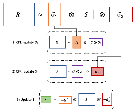
Figure 1: Schematic diagram of one iteration of the proposed triFastSTMF method for updating factor matrices $G_{1},S$ and $G_{2}$ of the data matrix $R\approx G_{1}\otimes S\otimes G_{2}$. Step 1) updates the factor matrix $G_{1}$ through CFL, while step 2) uses the new $G_{1}$ to update $G_{2}$ through CFR. The last step, 3) updates $S$ using Theorem 2 and newly-computed factor matrices $G_{1}$ and $G_{2}$. The procedure repeats until convergence.

1. We follow the results obtained in [12] to preprocess a data matrix into a suitable shape using transformations, like matrix transposition and random permutation of rows. Wide matrices are shown to achieve smaller errors compared to tall matrices [12].

2. The default initialization of factor matrices $G_{1}$, $S$ and $G_{2}$ uses the Random Acol strategy [11], which computes the element-wise average of randomly selected columns from matrix $R$. Fixed initialization for matrices $G_{1}$, $S$, and $G_{2}$ can be used straight from the data, see Section 4.2.

3. Until converged, each iteration of the algorithm first updates $G_{1}$ and $G_{2}$ using CFL and CFR, presented in Algorithms 2 and 3, respectively, and described below. Then we compute the middle factor $S$ as the greatest subsolution of equation $G_{1}\otimes S\otimes G_{2}=R$ by Theorem 2 as

   $$S=(-G_{1})^{T}\otimes^{*}R\otimes^{*}(-G_{2})^{T}.$$

4. As the last step of triFastSTMF, we reshape the factor matrices $G_{1}$, $S$ and $G_{2}$ into appropriate forms depending on the initial transformation of the data matrix $R$. If some of the elements of the data matrix $R$ are not given, we apply the operations proposed in [11] to skip all the missing values in the calculation.

Algorithm 1 Tri-factorization over the tropical semiring (triFastSTMF)

0:  data matrix $R$ $\in\mathbb{R}_{\max}^{m\times n}$, approximation ranks $r_{1}$, $r_{2}$

0:  factorization $G_{1}\in\mathbb{R}_{\max}^{m\times r_{1}}$, $S\in\mathbb{R}_{\max}^{r_{1}\times r_{2}}$, $G_{2}\in\mathbb{R}_{\max}^{r_{2}\times n}$

  if $R$ not wide then transpose $R$

  $perm\leftarrow$ random permutation of indices $1\dots m$

  $R\leftarrow R[perm,:]$

  initialize $G_{1},G_{2}$

  $S\leftarrow(-G_{1})^{T}\otimes^{*}R\otimes^{*}(-G_{2})^{T}$

  while not converged do

     $G_{1}\leftarrow CFL(R,G_{1},S,G_{2})$

     $G_{2}\leftarrow CFR(R,G_{1},S,G_{2})$

     $S\leftarrow(-G_{1})^{T}\otimes^{*}R\otimes^{*}(-G_{2})^{T}$

  if $R$ transposed then

  $(G_{1},S,G_{2})\leftarrow(G_{2}^{T},S^{T},G_{1}[perm^{-1},:]^{T})$

  else $(G_{1},S,G_{2})\leftarrow(G_{1}[perm^{-1},:],S,G_{2})$

  return  $G_{1},S,G_{2}$

Algorithm 2 Compute Factorization to update the Left factor matrix $G_{1}$ (CFL)

0:  data matrix $R$ $\in\mathbb{R}_{\max}^{m\times n}$, factor matrices: left $G_{1}\in\mathbb{R}_{\max}^{m\times r_{1}}$, middle $S\in\mathbb{R}_{\max}^{r_{1}\times r_{2}}$, and right $G_{2}\in\mathbb{R}_{\max}^{r_{2}\times n}$

0:  left factor matrix $G_{1}\in\mathbb{R}_{\max}^{m\times r_{1}}$

  $Q=S\otimes G_{2}$

  while not converged do

     for each row $i$ of $R$

        $err$, $row\_inds$, $col\_inds\leftarrow\text{TD\_A}(R,G_{1},Q,i)$

        for each $j$ in argsort(err) in decreasing order

           $k\leftarrow\operatorname*{argmax}_{\ell}\left({\rm count_{\ell}}\left(row\_inds\text{ }\cup\break\text{ }col\_inds[j]\right)\right)$

           $(G_{1},Q,G_{1(\cdot k)}^{\prime},Q_{k\cdot}^{\prime})\leftarrow\text{F-ULF}(R,G_{1},Q,i,j,k)$

           if $\left\lVert R-G_{1}\otimes S\otimes G_{2}\right\rVert_{b}$ decreases then break

           else $(G_{1(\cdot k)},Q_{k\cdot})\leftarrow(G_{1(\cdot k)}^{\prime},Q_{k\cdot}^{\prime})$

           $(G_{1},Q,G_{1(\cdot k)}^{\prime},Q_{k\cdot}^{\prime})\leftarrow\text{F-URF}(R,G_{1},Q,i,j,k)$

           if $\left\lVert R-G_{1}\otimes S\otimes G_{2}\right\rVert_{b}$ decreases then break

           else $(G_{1(\cdot k)},Q_{k\cdot})\leftarrow(G_{1(\cdot k)}^{\prime},Q_{k\cdot}^{\prime})$

  return  $G_{1}$

Algorithm 3 Compute Factorization to update the Right factor matrix $G_{2}$ (CFR)

0:  data matrix $R$ $\in\mathbb{R}_{\max}^{m\times n}$, factor matrices: left $G_{1}\in\mathbb{R}_{\max}^{m\times r_{1}}$, middle $S\in\mathbb{R}_{\max}^{r_{1}\times r_{2}}$, and right $G_{2}\in\mathbb{R}_{\max}^{r_{2}\times n}$

0:  right factor matrix $G_{2}\in\mathbb{R}_{\max}^{r_{2}\times n}$

  $Q=G_{1}\otimes S$

  while not converged do

     for each row $i$ of $R$

        $err$, $row\_inds$, $col\_inds\leftarrow\text{TD\_A}(R,Q,G_{2},i)$

        for each $j$ in argsort(err) in decreasing order

           $k\leftarrow\operatorname*{argmax}_{\ell}\left({\rm count_{\ell}}\left(row\_inds\text{ }\cup\break\text{ }col\_inds[j]\right)\right)$

           $(Q,G_{2},Q_{\cdot k}^{\prime},G_{2(k\cdot)}^{\prime})\leftarrow\text{F-ULF}(R,Q,G_{2},i,j,k)$

           if $\left\lVert R-G_{1}\otimes S\otimes G_{2}\right\rVert_{b}$ decreases then break

           else $(Q_{\cdot k},G_{2(k\cdot)})\leftarrow(Q_{\cdot k}^{\prime},G_{2(k\cdot)}^{\prime})$

           $(Q,G_{2},Q_{\cdot k}^{\prime},G_{2(k\cdot)}^{\prime})\leftarrow\text{F-URF}(R,Q,G_{2},i,j,k)$

           if $\left\lVert R-G_{1}\otimes S\otimes G_{2}\right\rVert_{b}$ decreases then break

           else $(Q_{\cdot k},G_{2(k\cdot)})\leftarrow(Q_{\cdot k}^{\prime},G_{2(k\cdot)}^{\prime})$

  return  $G_{2}$

Note that triFastSTMF updates one factor matrix at a time using CFL and CFR, presented in Algorithms 2 and 3, respectively. They are both based on FastSTMF and represent the two-factorization with FastSTMF core [12] that contains minor changes:

• In CFL/CFR, we remove the initialization of the factor matrices, as they are already initialized at the beginning of triFastSTMF. In CFL, we update only the left factor matrix $G_{1}$, and declare $Q=S\otimes G_{2}$ to be the second factor matrix. Similarly, in CFR, we update only the right factor matrix $G_{2}$ and $Q=G_{1}\otimes S$ is the first factor matrix. This approach prevents overfitting factor matrices since the optimization iterates over the left and right factorization. Such a process gives equal importance to both factor matrices, allowing patterns to spread in multiple factor matrices instead of being consolidated in one of them.

• We change the computation of the approximation error. FastSTMF computes the error of two-factorization, while CFL/CFR computes the tri-factorization error using the current factor matrices $G_{1}$, $S$, and $G_{2}$.

• We do not transpose the matrices nor permute the rows of matrices in CFL/CFR since this is performed as part of triFastSTMF.

The functions F-ULF, F-URF and TD-A used in CFL and CFR are the same as in the FastSTMF algorithm [12]. We present the pseudocode of TD-A in Algorithm 4, where the notation of functions used is given in [12].

Algorithm 4 TD_A

0:  data matrix $R$ $\in\mathbb{R}_{\max}^{m\times n}$, left factor matrix $U$, right factor matrix $V$, row $i$ of $R$

0:  $errors,row\_indices,column\_indices$

  $row\_indices\leftarrow\{\!\!\{f(i,t)\colon t=1,\ldots,n\}\!\!\}$

  errors, $columns\_indices\leftarrow[\,],[\,]$

  for each column $j$ of $R$

     $e\leftarrow\mathrm{td}_{col}(R,U,V,j)$

     append $e$ to errors

     $col\_indices\leftarrow\{\!\!\{f(t,j)\colon t=1,\ldots,m\}\!\!\}$

     append $col\_indices$ to $columns\_indices$

  return  $errors,row\_indices,column\_indices$

3.1.3 Different aspects of the tri-factorization on networks

The four-partition network shown in Figure 2 is an illustrative example of where we can apply tri-factorization for network structure analysis. We represent the four-partition network with three factor matrices which is the basis of tri-factorization methods. Further, different approaches to four-partition networks can be used depending on the nature of the data and the task that needs to be solved.

For a network $\Gamma$ with a vertex set

$$V(\Gamma)= \{x(i)\colon i=1,\ldots,m\}\cup\{y(j)\colon j=1,\ldots,r_{1}\}\cup$$

$$\{w(k)\colon k=1,\ldots,r_{2}\}\cup\{z(\ell)\colon\ell=1,\ldots,n\}$$

and an edge set $E(\Gamma)$, we define a matrix $G_{1}\in\mathbb{R}_{\max}^{m\times r_{1}}$ such that $G_{1(ij)}$ represents the weight on the edge from $x(i)$ to $y(j)$, a matrix $S\in\mathbb{R}_{\max}^{r_{1}\times r_{2}}$ where $S_{jk}$ represents the weight on the edge from $y(j)$ to $w(k)$ and a matrix $G_{2}\in\mathbb{R}_{\max}^{r_{2}\times n}$ where $G_{2(k\ell)}$ represents the weights of the edges from $w(k)$ to $z(\ell)$. Then $R=G_{1}\otimes S\otimes G_{2}$ is the $m\times n$ matrix such that

$$R_{i\ell}=\max_{1\leq j\leq r_{1},1\leq k\leq r_{2}}((G_{1})_{ij}+S_{jk}+(G_{2})_{k\ell})$$

is the length of the longest path from $x(i)$ to $z(\ell)$, see Figure 2. If a matrix $R$ is given, we can estimate $G_{1},S$ and $G_{2}$ with triFastSTMF.

Figure 2: Example of a four-partition network.

The main question is how to present an arbitrary network as a four-partition network. The two main approaches are:

• All nodes in the four-partition network are real nodes. The matrices $G_{1},S$, and $G_{2}$ represent weights of the real edges from the original network, which preserves the interpretability of the network since the relations are only between real nodes. Moreover, the size of the four-partition network remains the same size as the original network. This approach is suitable when the original network’s structure already has four partitions.

• Some nodes in the four-partition network are latent nodes. The real nodes are only outer nodes ($x,z$), while latent nodes are inner nodes ($y,w$). In this case, the matrices $G_{1},S$ and $G_{2}$ represent latent features of the outer nodes and not real weights from the original network, leading to a more difficult interpretability of the network since now the relations are also between real and latent nodes. The size of the four-partition network is larger than the size of the original network, which means increases the complexity of the task using this approach.

We focus on the first approach, where all nodes in the network are real nodes since we want to use the patterns from the data to initialize the factor matrices, maintain network interpretability, demonstrate how to work with real four-partition networks, and consequently obtain a better approximation of matrices $R,G_{1},S,G_{2}$. In this way, we fully present the power of tri-factorization over two-factorization and its primary purpose.

3.1.4 Comparison with other strategies

In our work, we developed different tropical tri-factorization strategies, triSTMF and Consecutive, that are based on two-factorizations [11, 12]. We compare their effectiveness with proposed triFastSTMF in Section 4.1.1.

The triSTMF strategy is based on the TD_A method from FastSTMF, and we implement triSTMF tri-factorization as two different two-factorizations:

1. Left factor matrix is $G_{1}\otimes S$, right factor matrix is $G_{2}$.

2. Left factor matrix is $G_{1}$, right factor matrix is $S\otimes G_{2}$.

We denote errors obtained from TD_A in the i) case as $\varepsilon_{L}$ and errors in the ii) case as $\varepsilon_{R}$. We developed two versions called triSTMF-BothTD and triSTMF-RandomTD, which differ in the order of how the error is computed. In triSTMF-BothTD, the computation is performed using both $\varepsilon_{L}$ and $\varepsilon_{R}$. The smaller error between $\varepsilon_{L}$ and $\varepsilon_{R}$ is selected to perform optimization. In contrast, triSTMF-RandomTD randomly computes $\varepsilon_{L}$ or $\varepsilon_{R}$ and continues with the optimization. Also, triSTMF uses ULF and URF from STMF as the basis for updating factor matrices. Note that we cannot use F-ULF and F-URF directly in the case of tri-factorization since the third factor matrix $S$ introduces additional complexity to F-ULF and F-URF, resulting in incompatible operations. This results in a slow optimization process of both versions of triSTMF.

The Consecutive strategy has two versions: lrConsecutive and rlConsecutive. The goal of this strategy is to achieve tri-factorization by first applying FastSTMF to the data matrix $R$, resulting in factor matrices $U$ and $V$. In the second step, lrConsecutive obtains the third factor matrix by applying FastSTMF to the matrix $V$ to obtain $S$ and $G_{2}$, while $G_{1}=U$. In contrast, rlConsecutive applies FastSTMF to the matrix $U$ to obtain $G_{1}$ and $S$, while $G_{2}=V$. The drawback of a consecutive strategy is the consolidation of the patterns in one of the factor matrices during the first step.

3.2 Synthetic data

We created a synthetic data matrix of size $200\times 100$ using the $(\max,+)$ multiplication of three random non-negative matrices. Since the purpose of synthetic data is to present the perfect scenario in which the proposed method works the best, we created our synthetic data using three random factor matrices of sufficiently large ranks $r_{1}=25$ and $r_{2}=20$. We use a synthetic data matrix to compare different tropical matrix factorization methods in Section 4.1.1. We also created a synthetic network with four partitions of sizes $(m,r_{1},r_{2},n)=(45,10,15,30)$ and use it to analyze four-partition network in Section 4.1.2.

3.3 Real data

We downloaded the real-world interaction dataset of an ant colony [27] from the Network Data Repository [28]. The nodes represent 160 ants, the edges represent physical contact (interaction), and the edge weight is the frequency of interaction during 41 days in total. We preprocessed the network to the appropriate format for evaluation as explained in Section 4.2. In Figure 3, we show the daily average frequency of interactions between ants. The distance between the nodes indicates the strength of interactions, i.e., nodes are closer when the interaction is stronger; contrary, nodes are farther apart when the interaction is weaker. The outer nodes interact less frequently with the nodes in the center of the network. We depict the individual frequency of interactions with the transparency of the edge color in Figure 3.

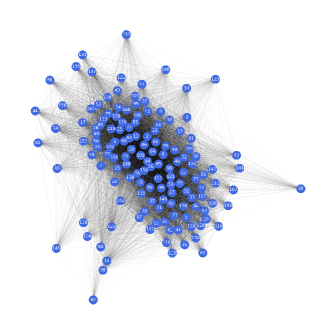
Figure 3: A real-world network of the daily average frequency of interactions in an ant colony. The strength of the interaction is visualized with the distance between nodes and edge transparency.

3.4 Evaluation metrics

In our work, we use the following metrics:

• Root-mean-square error or RMSE is a commonly used metric for comparing matrix factorization methods [12]. We use the RMSE in our experiments to evaluate the approximation error RMSE-A on the train data, and prediction error RMSE-P on the test data.

• $b$-norm is defined as $||W||_{b}=\sum_{i,j}|W_{ij}|$, and it is used in [11] and [12] as objective function. We also use the $b$-norm to minimize the approximation error of triFastSTMF.

• Rand score is a similarity measure between two clusterings that considers all pairs of samples and counts pairs assigned in the same or different clusters in the predicted and actual clusterings [29]. We use the Rand score to compare different partitioning strategies of the synthetic network.

3.5 Evaluation

We conducted experiments on synthetic data matrices with true ranks $r_{1}=25$ and $r_{2}=20$. The experiments were repeated $25$ times for $300$ seconds using Random Acol initialization.

For the synthetic four-partition network reconstruction, we repeat the experiments $25$ times using fixed initialization with different random and partially-random partitionings. Due to the smaller matrices, these experiments run for $100$ seconds.

For real data, we used the Louvain method [23] to obtain $r_{1}$ and $r_{2}$. Furthermore, we randomly removed at most $20\%$ of the edges. We use fixed initialization and run the experiments for $300$ seconds.

4 Results

We perform experiments on synthetic and real data. First, we compare different tropical matrix factorization methods on the synthetic data matrix and show that triFastSTMF achieves the best results of all tropical approaches. Next, we analyze the effect of different partitioning strategies on the performance of triFastSTMF. Finally, we evaluate the proposed triFastSTMF on real data and compare it with Fast-NMTF.

4.1 Synthetic data

4.1.1 Comparison between the tropical matrix factorization methods

We experiment with different two-factorization and tri-factorization tropical methods. The set of all tri-factorizations represent a subset of all two-factorizations. Specifically, each tri-factorization is also a two-factorization, meaning that, in general, we cannot obtain better approximation results with tri-factorization compared to two-factorization. In Figure 4, we see that the first half of lrConsecutive is better than the second half of lrConsecutive. Namely, in the first half, we perform two-factorization, while in the second half, we factorize one of the factor matrices to obtain three factor matrices as the final result. This second approximation introduces uncertainty and larger errors compared to the first half. We see a similar behavior in rlConsecutive. In this scenario, we show that the two-factorization is better than the tri-factorization. We see that the results of triSTMF-BothTD and triSTMF-RandomTD overlap and do not make any updates during the limited running time since they use slow algorithms to update factor matrices.

Comparing the two-factorization method FastSTMF and the tri-factorization method triFastSTMF, we obtain a similar approximation error in Figure 4. We see that our proposed triFastSTMF achieves the lowest approximation error on the synthetic data matrix of all tested tropical tri-factorization methods.

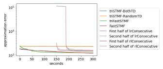
Figure 4: Comparison of different tropical tri-factorization methods. The median, first and third quartiles of the approximation error in 25 runs on the synthetic random tropical $200\times 100$ matrix are shown.

Tri-factorization may outperform two-factorization in a limited running time because of the nature of the data and the initialization of factor matrices. Theoretically, we expect that two-factorization and tri-factorization would achieve the same results when evaluated across a large number of datasets. Tri-factorization has demonstrated its superiority over two-factorization in many examples. An important application of tri-factorization is the fusion of data from different sources [3]. In our work, we show that tri-factorization can be applied to approximate and predict weights in four-partition networks.

4.1.2 Analysis of four-partition network construction

We construct a random tropical network $K$ of total $100$ nodes with a four-partition $A\cup B\cup C\cup D$. We denote the sizes of sets $A$, $B$, $C$ and $D$ as $m$, $r_{1}$, $r_{2}$ and $n$, respectively, and choose $(m,r_{1},r_{2},n)=(45,10,15,30)$, see Figure 5. We want to check the robustness of proposed triFastSTMF to the partitioning process and answer the following question: Is approximation error stable among different choices of partitioning?

Network $K$ contains the following edges:

• edges from $A$ to $B$, denoted as $A-B$, have weights represented by a random matrix $M_{1}^{m\times r_{1}}$,

• edges from $B$ to $C$, denoted as $B-C$, have weights represented by a random matrix $T^{r_{1}\times r_{2}}$,

• edges from $C$ to $D$, denoted as $C-D$, have weights represented by a random matrix $M_{2}^{r_{2}\times n}$,

• edges from $A$ to $D$, denoted as $A-D$, have weights represented by matrix $E=M_{1}\otimes T\otimes M_{2}$.

We propose the following general algorithm for converting the input network $K$ into a suitable form for tri-factorization. First, partition all network nodes into four sets, $X,Y,W$, and $Z$, with fixed sizes $m,r_{1},r_{2}$ and $n$, respectively, in two ways:

• random partitioning: $X\cup Y\cup W\cup Z$ is a random four-partition of the chosen size. Random partitioning is a valid choice when all network nodes represent only one type of object. For example, in a social network, a node represents a person.

• partially-random partitioning: $Y,W$ are random subsets of nodes of $K$ of sizes $r_{1}$ and $r_{2}$, while $X=A$ and $Z=D$, where $A,D$ are given. Partially-random partitioning is applicable when there are two types of objects represented in the network. For example, in the movie recommendation system, users belong to the set $X$ and movies to $Z$. In this case, sets $Y$ and $W$ represent the latent features of $X$ and $Z$.

See examples of random and partially-random partitioning in Figure 5, where we show only the edges $X-Y$, $Y-W$ and $W-Z$ to achieve easier readability of the network. Given the (pseudo)random partitioning, construct matrix $R$ as the edges $X-Z$. The matrices $G_{1},S$ and $G_{2}$ are constructed as explained in 3.1.3 and can be used for the initialization of tri-factorization of $R$ (fixed initialization). For the missing edges, we set the corresponding values in triFastSTMF to be a random number from elements of $G_{1},S$ and $G_{2}$. Tri-factorization on $R$ will return updated $R,G_{1},S,G_{2}$ with approximated/predicted weights on edges.

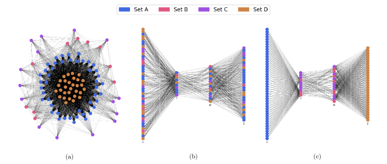
Figure 5: (a) A synthetic random tropical network $K$ of 100 nodes created by applying the tropical semiring on four sets $A,B,C$ and $D$. The sets $A$ and $D$ are densely connected, following the network construction process. In contrast, sets $B$ and $C$ are less connected. Example of partitioning network $K$, using b) random and c) partially-random partitioning.

We show that partially-random partitioning achieves higher Rand scores, but approximation errors are similar to the ones obtained by random partitioning, see Figure 6. We conclude that the partitioning process does not significantly affect the approximation error of triFastSTMF. Still, if there is some additional knowledge about the sets of partition, it is better to use partially-random partitioning. When we do not know the real partition, random partitioning or advanced algorithms, such as the Louvain method, can be used.

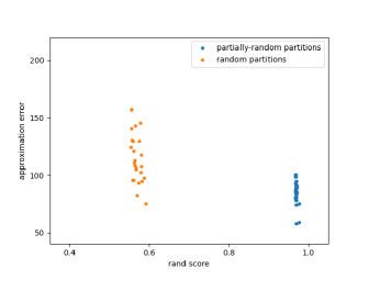
Figure 6: Rand score and approximation error of triFastSTMF on 25 random and 25 partially-random partitionings of synthetic data. We performed one run of 100 seconds for each matrix $R$ and used true ranks $r_{1}$ and $r_{2}$ as factorization parameters.

4.2 Real data

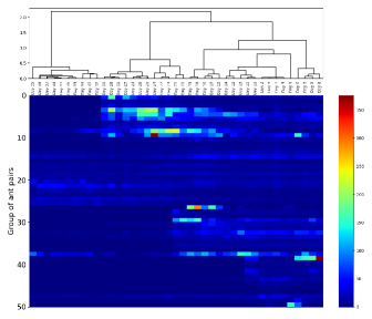
Figure 7: Analysis of ants’ behavioral patterns over 41 days. The rows represent centroids of clustered ant pairs with k-means using $k=50$, and the columns denote daily interactions. Rows and columns are ordered using Optimal Leaf Ordering for Hierarchical Clustering [30] using cosine distance and Ward linkage.

We test our method on a real-world interaction dataset of ant colony introduced in Section 3.3. We describe the data on the interaction between pairs of ants using a weighted adjacency matrix of size $160\times 160$, where diagonal elements are equal to $0$. The adjacency matrix is symmetric, and we use the data from the upper triangular part to construct the matrix $H$, where each row describes one pair of ants, and columns represent a specific day. Since $H$ is large, we use k-means clustering to obtain 50 clusters and analyze the behavioral patterns of the ants on each day, shown in Figure 7.

There are three groups of days with different dynamics of ant interaction: $D_{1}$ represents days $1-19$, $D_{2}$ are days $20-31$, and $D_{3}$ are days $32-41$. We preprocessed the data for each group of days $D_{1}$, $D_{2}$ and $D_{3}$ such that the corresponding weight between two ants represents the daily average of all interactions for the specific days, see Figure 8.

The group $D_{2}$, which contains days $20-31$ and $140$ pairs of ants with positive weights, is the most dynamic of the three groups and has local communities. We construct a network $N$ from the group $D_{2}$, where the nodes represent individual ants, and the weight of the edges represents the strength of interactions between ants. The network density of $N$ is $88\%$. The weighted adjacency matrix of $N$ is denoted as $A$.

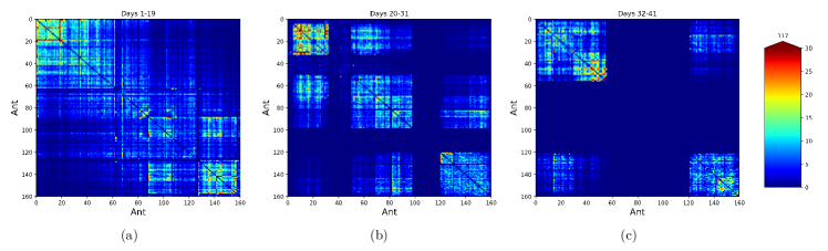
Figure 8: Comparison between the daily average of all interactions between ant pairs for different groups of days: (a) days 1-19, (b) days 20-31, and (c) days 32-41. Rows and columns are ordered using Optimal Leaf Ordering for Hierarchical Clustering [30] using cosine distance and Ward linkage.

Next, we construct ten different networks, $N_{1},\dots,N_{10}$ by sampling with replacement the edges from $N$. Each sampled network has at most $20\%$ of missing edges from $N$, which are used for evaluation. For each network $N_{i}$, $i\in\{1,\ldots,10\}$, we construct the weighted adjacency matrix $A_{i}$ with the exact same size and ordering of the nodes in rows and columns as in matrix $A$. Now, to apply tri-factorization on networks, we need to perform Louvain partitioning [23] for each $N_{i}$ to obtain a four-partition of its nodes: $X_{i}\cup Y_{i}\cup W_{i}\cup Z_{i}$.

Louvain method assigns sets of a four-partition and enables favoring larger communities using parameter $\gamma$. Different partitions are obtained for different values of $\gamma$, from which we select a connected four-partition network. We prefer the outer sets $X_{i}$ and $Z_{i}$ of corresponding sizes $m$ and $n$, respectively, to have a larger size than the inner sets $Y_{i}$ and $W_{i}$ of sizes $r_{1}$ and $r_{2}$, respectively. This will ensure that the matrix factorization methods embed data into low-dimensional space using rank values $r_{1},r_{2}\ll\min\{m,n\}$. Louvain algorithm results in different parameters $m,r_{1},r_{2}$ and $n$ for each $N_{i}$, $i\in\{1,\ldots,10\}$, shown in Table 1. We define $\mu$ to represent a percentage of nodes in outer sets. Table 1 shows that $\mu\geq 74\%$ for all $N_{i}$. We construct $R_{i}$ matrices of corresponding sizes $m\times n$ using edges from $X_{i}$ to $Z_{i}$, and the corresponding matrices $G_{1},S$ and $G_{2}$ of sizes $m\times r_{2}$, $r_{1}\times r_{2}$ and $r_{2}\times n$, respectively, using all four sets. In $R_{i}$, we mask all values equal to $0$.

Network	$m$	$r_{1}$	$r_{2}$	$n$	$\mu$
$N_{1}$	$65$	$21$	$2$	$52$	$84\%$
$N_{2}$	$57$	$22$	$5$	$56$	$81\%$
$N_{3}$	$57$	$24$	$2$	$57$	$81\%$
$N_{4}$	$60$	$21$	$2$	$57$	$84\%$
$N_{5}$	$60$	$20$	$4$	$56$	$83\%$
$N_{6}$	$61$	$19$	$2$	$58$	$85\%$
$N_{7}$	$57$	$18$	$15$	$50$	$76\%$
$N_{8}$	$52$	$23$	$14$	$51$	$74\%$
$N_{9}$	$67$	$4$	$2$	$67$	$96\%$
$N_{10}$	$65$	$15$	$2$	$58$	$88\%$

Table 1: Louvain partitioning of $N_{i}$ where $i\in[1,10]$, containing $140$ nodes from days $20-31$.

We run matrix factorization methods on each $R_{i}$ matrix using the corresponding factor matrices $G_{1},S,$ and $G_{2}$ for fixed initialization and obtain updated matrices $G_{1},S,$ and $G_{2}$. Since we use fixed initialization, we evaluate each method only once because there is no presence of randomness. In Table 2, we present the comparison between our proposed triFastSTMF and Fast-NMTF. The results show that Fast-NMTF achieves a smaller approximation error RMSE-A, while triFastSTMF outperforms Fast-NMTF in a better prediction error RMSE-P. This result is consistent with previous research in [11] and [12], where we have shown that matrix factorization over the tropical semiring is more robust to overfitting compared to methods using standard linear algebra.

Metric	Method	$R_{1}$	$R_{2}$	$R_{3}$	$R_{4}$	$R_{5}$	$R_{6}$	$R_{7}$	$R_{8}$	$R_{9}$	$R_{10}$
RMSE-P	triFastSTMF	1.90	1.07	2.32	1.09	1.15	1.78	0.88	0.88	1.38	2.05
	Fast-NMTF	0.93	1.25	1.42	1.11	1.21	0.82	1.17	1.10	1.48	1.59
RMSE-A	triFastSTMF	1.90	0.90	2.34	1.23	1.02	1.64	0.92	0.69	1.33	2.12
	Fast-NMTF	0.54	0.37	0.49	0.52	0.43	0.53	0.17	0.17	0.80	0.58

Table 2: RMSE-A and RMSE-P on data matrices $R_{i}$. The result of the best method in the comparison between triFastSTMF and Fast-NMTF is shown in bold.

Metric	Method	$N_{1}$	$N_{2}$	$N_{3}$	$N_{4}$	$N_{5}$	$N_{6}$	$N_{7}$	$N_{8}$	$N_{9}$	$N_{10}$
RMSE-P	triFastSTMF	9.43	11.40	12.76	10.35	10.99	8.56	10.63	12.85	7.56	9.28
	Fast-NMTF	7.24	3602725.48	6.21	7.09	289129.41	116821.55	12733965.01	763401.17	6.24	6.18
RMSE-A	triFastSTMF	8.43	9.95	12.37	9.63	10.10	8.50	10.20	11.90	7.35	8.75
	Fast-NMTF	6.07	1034154.82	6.22	6.02	339449.43	118555.72	13423203.65	691714.60	6.02	6.15

Table 3: RMSE-A and RMSE-P on network $N$ using different partitions of $N_{i}$. The result of the best method in the comparison between triFastSTMF and Fast-NMTF is shown in bold.

The matrix $R_{i}$ contains only edges $X_{i}-Z_{i}$. All other edges $X_{i}-Y_{i}$, $Y_{i}-W_{i}$ and $W_{i}-Z_{i}$ are hidden in the corresponding factor matrices $G_{1},S$ and $G_{2}$. If we want to obtain predictions for all edges of network $N$ using different partitions of $N_{i}$, we need to also consider factor matrices, not just matrix $R_{i}$. To achieve this, we take into account the corresponding $G_{1},S$ and $G_{2}$ including their products $G_{1}\otimes S$, $S\otimes G_{2}$ and $G_{1}\otimes S\otimes G_{2}$. The edges that were removed from $N$ during the sampling process to obtain $N_{i}$ are used to measure the prediction error, while the edges in $N_{i}$ are used for approximation.

In Table 3, we present the comparison between our proposed triFastSTMF and Fast-NMTF on network $N$ using different partitions of $N_{i}$. The results show that triFastSTMF and Fast-NMTF have the same number of wins regarding the RMSE-A and RMSE-P. However, the main difference between triFastSTMF and Fast-NMTF is in the fact that Fast-NMTF achieves an enormous error compared to triFastSTMF in half of the cases. This is because now we are also predicting edges $X_{i}-Y_{i},Y_{i}-W_{i},W_{i}-Z_{i}$ and $X_{i}-W_{i},Y_{i}-Z_{i}$, which we obtain by multiplying the corresponding factor matrices $G_{1},S$ and $G_{2}$ properly. There is no guarantee that the factor matrices $G_{1},S$, and $G_{2}$ and their products are on the same scale as the data matrix $R_{i}$ on which the matrix factorization methods were trained. Since Fast-NMTF uses standard linear algebra, one more matrix multiplication is needed to get to the original data scale. Using standard $+$ and $\times$ operators results in significant error, since the predicted values expand in magnitude quickly. triFastSTMF does not have this problem because it is based on tropical semiring, and the operators $\max$ and $+$ are more averse to predicting large values.

5 Conclusion

Matrix factorization is a popular data embedding approach used in various machine learning applications. Most factorization methods use standard linear algebra. Recent research introduced tropical semiring to matrix factorization, which enables the modeling of nonlinear relations. Two-factorization approaches are often applied to study bipartite and tripartite networks. However, tri-factorization is suitable for application on four-partition networks, and to the best of our knowledge, our work is the first to explore this option.

In this study, we evaluate different strategies based on two-factorization, called triSTMF and Consecutive. Both strategies have different drawbacks, such as a slow optimization process in triSTMF and the overfitting of one of the factor matrices in Consecutive. These limitations have motivated us to develop a novel tri-factorization approach that addresses the limitations of triSTMF and Consecutive. We propose triFastSTMF, a tri-factorization algorithm over the tropical semiring that can be used for a single data source. Our proposed algorithm is based on FastSTMF, a two-factorization method, with the necessary modifications for tri-factorization. We also provide a detailed theoretical analysis for solving the linear system and computing the third factor matrix. The obtained solution is used for the optimization in the proposed triFastSTMF.

We tested the method on synthetic and real data, applied it to the edge approximation and prediction task in four-partition networks and demonstrated that triFastSTMF achieves close approximation and prediction results as Fast-NMTF. Additionally, triFastSTMF is more robust than Fast-NMTF in cases when methods are fitted on a part of the network and then used to approximate and predict the entire network.

Although in this study we presented the proposed method on a single data source, we established the basis for creating a model capable of combining multiple data sources. Our future work involves the application and modification of the proposed triFastSTMF to the data fusion problem, which often employs tri-factorization.

Supporting information

The supporting Python notebooks and the data are available on GitHub https://github.com/Ejmric/triFastSTMF. We downloaded the real-world interaction dataset of an ant colony named insecta-ant-colony3 from Animal Social Networks data collection on http://networkrepository.com.

Author’s contributions

AO, PO and TC designed the study. AO wrote the software application and performed experiments. AO, PO, and TC analyzed and interpreted the results on synthetic and real data. AO wrote the initial draft of the paper. All authors edited and approved the final manuscript.

Declaration of competing interest

The authors declare that they have no known competing financial interests or personal relationships that could have appeared to influence the work reported in this paper.

Funding

This work is supported by the Slovene Research Agency, Young Researcher grant (52096) awarded to AO, and Research Program funding P1-0222 to PO and P2-0209 to TC.

References

- [1] Yehuda Koren, Robert Bell, and Chris Volinsky. Matrix factorization techniques for recommender systems. Computer, 42(8):30–37, 2009.
- [2] Weixiang Liu, Nanning Zheng, and Qubo You. Nonnegative matrix factorization and its applications in pattern recognition. Chinese Science Bulletin, 51:7–18, 2006.
- [3] Marinka Žitnik and Blaž Zupan. Data fusion by matrix factorization. IEEE transactions on pattern analysis and machine intelligence, 37(1):41–53, 2015.
- [4] James Hook. Linear regression over the max-plus semiring: algorithms and applications. arXiv preprint arXiv:1712.03499, ,, 2017.
- [5] Sanjar Karaev, James Hook, and Pauli Miettinen. Latitude: A model for mixed linear-tropical matrix factorization. In Proceedings of the 2018 SIAM International Conference on Data Mining, pages 360–368. SIAM, 2018.
- [6] Sanjar Karaev and Pauli Miettinen. Capricorn: An algorithm for subtropical matrix factorization. In Proceedings of the 2016 SIAM International Conference on Data Mining, pages 702–710. SIAM, 2016.
- [7] Sanjar Karaev and Pauli Miettinen. Algorithms for approximate subtropical matrix factorization. arXiv preprint arXiv:1707.08872, 2017.
- [8] Daniel D Lee and H Sebastian Seung. Learning the parts of objects by non-negative matrix factorization. Nature, 401(6755):788, 1999.
- [9] Zhongyuan Zhang, Tao Li, Chris Ding, and Xiangsun Zhang. Binary matrix factorization with applications. In Seventh IEEE International Conference on Data Mining (ICDM 2007), pages 391–400. IEEE, 2007.
- [10] Andriy Mnih and Russ R Salakhutdinov. Probabilistic matrix factorization. In Advances in neural information processing systems, pages 1257–1264, 2008.
- [11] Amra Omanović, Hilal Kazan, Polona Oblak, and Tomaž Curk. Sparse data embedding and prediction by tropical matrix factorization. BMC bioinformatics, 22(1):1–18, 2021.
- [12] Amra Omanović, Polona Oblak, and Tomaž Curk. FastSTMF: Efficient tropical matrix factorization algorithm for sparse data. arXiv preprint arXiv:2205.06619, 2022.
- [13] Sanjar Karaev and Pauli Miettinen. Cancer: Another algorithm for subtropical matrix factorization. In Joint European Conference on Machine Learning and Knowledge Discovery in Databases, pages 576–592. Springer, 2016.
- [14] Jason Weston, Ron J Weiss, and Hector Yee. Nonlinear latent factorization by embedding multiple user interests. In Proceedings of the 7th ACM conference on Recommender systems, pages 65–68, 2013.
- [15] Thanh Le Van, Siegfried Nijssen, Matthijs Van Leeuwen, and Luc De Raedt. Semiring rank matrix factorization. IEEE Transactions on Knowledge and Data Engineering, 29(8):1737–1750, 2017.
- [16] Liwen Zhang, Gregory Naitzat, and Lek-Heng Lim. Tropical geometry of deep neural networks. In Jennifer Dy and Andreas Krause, editors, Proceedings of the 35th International Conference on Machine Learning, volume 80 of Proceedings of Machine Learning Research, pages 5824–5832, Stockholmsmässan, Stockholm Sweden, 10–15 Jul 2018. PMLR.
- [17] Guangyuan Fu, Jun Wang, Carlotta Domeniconi, and Guoxian Yu. Matrix factorization-based data fusion for the prediction of lncRNA–disease associations. Bioinformatics, 34(9):1529–1537, 2018.
- [18] Hua Wang, Feiping Nie, Heng Huang, and Fillia Makedon. Fast nonnegative matrix tri-factorization for large-scale data co-clustering. In Twenty-Second International Joint Conference on Artificial Intelligence, 2011.
- [19] Marinka Žitnik, Vuk Janjić, Chris Larminie, Blaž Zupan, and Nataša Pržulj. Discovering disease-disease associations by fusing systems-level molecular data. Scientific reports, 3(1):1–9, 2013.
- [20] Andrej Čopar, Blaž Zupan, and Marinka Žitnik. Fast optimization of non-negative matrix tri-factorization. PloS one, 14(6):e0217994, 2019.
- [21] Bart De Schutter and Bart De Moor. Matrix factorization and minimal state space realization in the max-plus algebra. In Proceedings of the 1997 American Control Conference (Cat. No. 97CH36041), volume 5, pages 3136–3140. IEEE, 1997.
- [22] Stefan Hougardy. The Floyd–Warshall algorithm on graphs with negative cycles. Information Processing Letters, 110(8-9):279–281, 2010.
- [23] Vincent D Blondel, Jean-Loup Guillaume, Renaud Lambiotte, and Etienne Lefebvre. Fast unfolding of communities in large networks. Journal of statistical mechanics: theory and experiment, 2008(10):P10008, 2008.
- [24] G David Forney. The Viterbi algorithm. Proceedings of the IEEE, 61(3):268–278, 1973.
- [25] Emmanouil Theodosis and Petros Maragos. Analysis of the Viterbi algorithm using tropical algebra and geometry. In 2018 IEEE 19th International Workshop on Signal Processing Advances in Wireless Communications (SPAWC), pages 1–5. IEEE, 2018.
- [26] Stephane Gaubert and Max Plus. Methods and applications of (max,+) linear algebra. In Annual symposium on theoretical aspects of computer science, pages 261–282. Springer, 1997.
- [27] Danielle P Mersch, Alessandro Crespi, and Laurent Keller. Tracking individuals shows spatial fidelity is a key regulator of ant social organization. Science, 340(6136):1090–1093, 2013.
- [28] Ryan A. Rossi and Nesreen K. Ahmed. The network data repository with interactive graph analytics and visualization. In AAAI, 2015.
- [29] Lawrence Hubert and Phipps Arabie. Comparing partitions. Journal of classification, 2:193–218, 1985.
- [30] Ziv Bar-Joseph, David K Gifford, and Tommi S Jaakkola. Fast optimal leaf ordering for hierarchical clustering. Bioinformatics, 17(suppl_1):S22–S29, 2001.