Dropout Regularization in Extended Generalized Linear Models based on Double Exponential Families

¹Chair of Uncertainty Quantification and Statistical Learning, Research Center Trustworthy Data Science and Security (UA Ruhr) and Department of Statistics (Technische Universität Dortmund)
²Department of Statistics and Data Science, National University of Singapore
^∗ Correspondence should be directed to Prof. Dr. Nadja Klein, Chair of Uncertainty Quantification and Statistical Learning, Research Center Trustworthy Data Science and Security (UA Ruhr) and Department of Statistics (Technische Universität Dortmund), Joseph-von-Fraunhofer-Str. 25, 44227 Dortmund, Germany.

Acknowledgments: Nadja Klein acknowledges support through the Emmy Noether grant KL 3037/1-1 of the German research foundation (DFG). This work has been partly supported by the Research Center Trustworthy Data Science and Security, one of the Research Alliance centers within the UA Ruhr

Even though dropout is a popular regularization technique, its theoretical properties are not fully understood. In this paper we study dropout regularization in extended generalized linear models based on double exponential families, for which the dispersion parameter can vary with the features. A theoretical analysis shows that dropout regularization prefers rare but important features in both the mean and dispersion, generalizing an earlier result for conventional generalized linear models. Training is performed using stochastic gradient descent with adaptive learning rate. To illustrate, we apply dropout to adaptive smoothing with B-splines, where both the mean and dispersion parameters are modelled flexibly. The important B-spline basis functions can be thought of as rare features, and we confirm in experiments that dropout is an effective form of regularization for mean and dispersion parameters that improves on a penalized maximum likelihood approach with an explicit smoothness penalty.

Keywords: Dropout regularization, generalized linear models, overdispersion and underdispersion, double exponential families, nonparametric estimation and B-splines

1 Introduction

Dropout regularization (Hinton et al., 2012; Srivastava et al., 2014) was introduced in the context of neural networks and has been successfully implemented in a large number of applications (Van Erven et al., 2014; Merity et al., 2017; Tan and Le, 2019). In its original formulation, dropout omits a randomly chosen subset of features during each iteration of stochastic gradient descent (SGD) optimization of the training loss. It has been generalized in various ways, and is an example of a broader class of methods using randomly corrupted features in model training (e.g Burges and Schölkopf (1996); Maaten et al. (2013)).

This work considers dropout for extended generalized linear models (GLMs) based on double exponential families (DEFs). The DEF was introduced by Efron (1986) and generalizes the natural exponential family (EF) by incorporating an additional dispersion parameter. Efron (1986) also developed regression models where the distribution of the output follows a DEF, and both the the mean and dispersion can vary with the features. The extended GLMs of Efron (1986) are related to extended quasi-likelihood methods (Lee and Nelder, 2000) and are particularly useful for count data. If count data are modelled using a binomial or Poisson distribution, then there is no separate scale parameter, and the variance is a function of the mean. For real count data, the variance can be more or less than expected based on a binomial or Poisson mean-variance relationship. If the variance is larger than expected, this is referred to as overdispersion (McCullagh and Nelder, 1998) and not taking it into account can result in unreliable inference (Dunn and Smyth, 2018). Underdispersion, where the variance is less than expected, can also occur, but is less common. McCullagh and Nelder (1998) state that it should be assumed that overdispersion is present unless proven otherwise. Extended GLMs for double binomial or double Poisson distributions are suitable alternatives to standard GLMs for count data exhibiting over- or underdispersion. We use dropout regularization in the mean and the dispersion to avoid overfitting and to prevent co-adaptation of features (Helmbold and Long, 2015).

In conventional GLMs with canonical link functions, Wager et al. (2013) have shown that dropout performs regularization which is first-order equivalent to L2 regularization, with a penalty matrix related to the empirical Fisher information. The form of the penalty favors rare but important features. In the neural network literature, previous work by Bishop (1995) has shown that adding Gaussian noise to the training data is equivalent to L2 regularization (also known as Tikhonov regularization). Baldi and Sadowski (2013) analyze dropout for both linear and non-linear networks, obtaining related results. Wang and Manning (2013) consider fast dropout based on analytically marginalizing the dropout noise. Wei et al. (2020) consider deep network architectures and identify both explicit and implicit regularization effects of dropout training, where the explicit effect of regularization is approximated by an L2 penalty term. Despite the connections between L2 regularization and dropout, dropout can behave very differently from both L1 and L2 regularization in some circumstances (Helmbold and Long, 2015).

Our work generalizes the study of Wager et al. (2013) to extended GLMs based on DEFs. Our first contribution is to give a theoretical analysis of the behaviour of dropout for extended GLMs. We discuss the way that the regularization parameters for the mean and dispersion models interact, and the effect of over- or underdispersion on the regularization of the mean. Our second contribution is to consider the use of dropout regularization in nonparametric estimation of extended GLMs with B-splines, and to compare dropout with penalized maximum likelihood estimation (PMLE) in this setting (Gijbels et al., 2010). Gijbels et al. (2010) consider an explicit smoothness penalty based on second-order difference operators for regularization (Eilers and Marx, 1996). Based on our theoretical analysis, in situations where highly adaptive regularization is required, the important B-spline basis functions can be thought of as rare features, matching the setting where dropout should work well. We confirm this in experiments, and also verify that performance improves when there is only overdispersion and no underdispersion.

In the rest of the paper, Section 2 introduces the extended GLM based on DEFs, Section 3 analyzes the regularization induced by dropout in this model class, and an application to adaptive smoothing with B-splines is discussed in Section 4. Section 5 gives a concluding discussion.

2 Generalized linear models based on double exponential families

2.1 Double exponential family

The distribution of a random vector $Y$ is in a natural EF if its target density has the form

$$f_{\theta}(y)=\exp\left(\langle\theta,y\rangle-b(\theta)+c(y)\right),$$ (1)

where $c(y)=\log h(y)$ and $b(\theta)=\log C(\theta)^{-1}$ for known functions $C(\cdot)$ and $h(\cdot)$. The EF is parameterized through $\theta\in\Theta$. When $Y$ is a random variable with density (1), $\mu:=\mathbb{E}_{\theta}[Y]=b^{\prime}(\theta)$ and $\mathbb{V}_{\theta}[Y]=b^{\prime\prime}(\theta)$, i.e.

$$\mathbb{V}_{\theta}[Y]=\frac{\partial}{\partial\theta}\mathbb{E}_{\theta}[Y].$$

This shows that the variance is determined by the mean function. Many popular distributions such as the Gaussian, Poisson and binomial have densities of the form (1). As discussed earlier, the implied mean-variance relationship for binomial and Poisson models may be inappropriate for real data, since for the Poisson distribution $\mathbb{V}_{\theta}(Y)=\mathbb{E}_{\theta}(Y)$, and for a binomial distribution with $N$ trials $\mathbb{V}(Y)=\mathbb{E}(Y)(N-\mathbb{E}(Y))/N$. For a general introduction and more details on EFs we refer to Lehmann and Casella (1998).

Efron (1986) extends the notion of the EF to the double exponential family (DEF) by introduction of a dispersion parameter $\gamma>0$. Target densities in the DEF are of the form

$$f_{\gamma,\theta}(y):=C(\gamma,\theta)\gamma^{\frac{1}{2}}f_{\theta}(y)^{\gamma}f_{\theta(y)}(y)^{1-\gamma},$$ (2)

where $f_{\theta}$ and $f_{\theta(y)}$ are densities as in (1), $C$ is a normalizing constant and $\theta(y)=(b^{\prime})^{-1}(y)$ is the value of $\theta$ for which the mean is $y$, and we allow $\theta(y)\in\mathbb{R}\cup\{-\infty,\infty\}$ to deal with boundary cases. The introduction of the dispersion parameter $\gamma$ decouples the mean and variance of the underlying natural EF and Efron (1986) shows that for a random variable $Y\sim\text{DEF}(\theta,\gamma)$ with density (2), $\mathbb{E}[Y]\approx\mu$, $\mathbb{V}[Y]\approx b^{\prime\prime}(\theta)/\gamma$ and $C(\gamma,\theta)\approx 1$; see Efron (1986) for further discussion of the accuracy of these approximations. From the expression for the variance, $\gamma<1$ ($\gamma>1$) corresponds to overdispersion (underdispersion). Also, we will assume that the map $\theta\mapsto b^{\prime}(\theta)$ is one-to-one, such that we can parameterize via $\mu$ instead of $\theta$. We will write $f_{\gamma,\mu}$ and $Y\sim\text{DEF}(\mu,\gamma)$ instead of $f_{\gamma,\theta}$ and $Y\sim\text{DEF}(\theta,\gamma)$.

2.2 GLMs based on DEFs

Consider observed data $\{(y_{i},\bm{x}_{i},\bm{z}_{i})\}_{i=1}^{n}$ of responses $y_{i}\in\mathcal{Y}\subseteq\mathbb{R}$ and feature vectors $\bm{x}_{i}\in\mathbb{R}^{d_{\mu}}$ and $\bm{z}_{i}\in\mathbb{R}^{d_{\gamma}}$. Conditionally on the features, the responses will be modelled as observations of independent random variables $Y_{i}$ with distributions from a DEF. The features $\bm{x}_{i}$ and $\bm{z}_{i}$ will appear in models for the mean and dispersion respectively. In the regression context it is convenient to rewrite the natural EF target density (1) for scalar $Y_{i}$ as

$$f_{\theta,\phi/\nu_{i}}(y_{i}) =\exp\left(\frac{\theta_{i}y_{i}-b(\theta_{i})}{\phi/\nu_{i}}+c\left(y_{i},\phi/\nu_{i}\right)\right),$$ (3)

where $\phi$ is a fixed scale parameter, $\nu_{i}$ is a known weight and both $\nu_{i}$ and $\theta_{i}$ can vary between observations. The mean for density (3) is $\mu_{i}=b^{\prime}(\theta_{i})$, and the variance is $(\phi/\nu_{i})b^{\prime\prime}(\theta_{i})$. For a conventional GLM with a binomial response such as a logistic regression, the weight $\nu_{i}$ would be $n_{i}$, the number of binomial trials for the $i$th observation. For binomial and Poisson GLMs the scale $\phi$ is $1$, but in a Gaussian linear regression the scale parameter $\phi$ is the response variance.

We leave dependence of all quantities on $\phi/\nu_{i}$ implicit in our notation in the following discussion, retaining our previously established notation for DEFs. In our extended GLMs based on DEFs, we assume

$$Y_{i}\,|\,\theta_{i},\gamma_{i}\sim\text{DEF}(\theta_{i},\gamma_{i}),$$

where, as discussed below, $\theta_{i}$ and $\gamma_{i}$ are functions of $\bm{x}_{i}$ and $\bm{z}_{i}$ respectively. Following Efron (1986), the DEF assumption implies

$$\mu_{i} :=\mathbb{E}[Y_{i}\,|\,\theta_{i},\gamma_{i}]\approx b^{\prime}(\theta_{i}),$$

$$\sigma^{2}_{i} :=\mathbb{V}[Y_{i}\,|\,\theta_{i},\gamma_{i}]\approx\frac{\phi b^{\prime\prime}(\theta_{i})}{\gamma_{i}\nu_{i}},$$

and $C(\gamma_{i},\theta_{i})\approx 1$. We take $\mu_{i}$ and $\gamma_{i}$ to be functions of linear predictors $\bm{x}_{i}^{T}\bm{\beta}$ and $\bm{z}_{i}^{T}\bm{\alpha}$, where $\bm{\beta}\in\mathbb{R}^{d_{\mu}}$ and $\bm{\alpha}\in\mathbb{R}^{d_{\gamma}}$ are unknown coefficient vectors. We choose a canonical link in the mean and a log link for the dispersion so that

$$\theta_{i}=(b^{\prime})^{-1}(\mu_{i}) =\bm{x}_{i}^{T}\bm{\beta},$$

$$\log(\gamma_{i}) =\bm{z}_{i}^{T}\bm{\alpha}.$$

The log link for the dispersion ensures the dispersion parameter is nonnegative.

3 Dropout regularization in GLMs based on DEFs

3.1 Dropout regularization

Dropout regularization randomly perturbs the observed feature vectors. Given some noise vector $\bm{\xi}$ and a noise function $\nu$, an observed feature vector $\bm{x}\in\mathbb{R}^{d}$ is transformed into $\widetilde{\bm{x}}:=\nu(\bm{x},\bm{\xi})$. The random perturbation is unbiased, which means that $\mathbb{E}(\widetilde{\bm{x}})=x$. In what follows we use multiplicative noise, $\nu(\bm{x},\bm{\xi})=\bm{x}\odot\bm{\xi}$, where $\odot$ is the elementwise product of two vectors. Assuming $\mathbb{E}[\bm{\xi}]=\bm{1}_{d}$, we have $\mathbb{E}[\widetilde{\bm{x}}]=\bm{x}\odot\mathbb{E}[\bm{\xi}]=\bm{x}$.

Typical choices for $\bm{\xi}$ include Bernoulli dropout with $\xi_{j}\stackrel{{\scriptstyle iid}}{{\sim}}(1-\delta)^{-1}\text{Bernoulli}(1-\delta)$, where $\delta\in(0,1)$ is the dropout probability, and Gaussian dropout with $\xi_{j}\stackrel{{\scriptstyle iid}}{{\sim}}\mathcal{N}(1,\sigma^{2})$, with noise variance $\sigma^{2}$, for $j=1\ldots,d$. We have described the process of random perturbation for a single feature vector. With many feature vectors, different random perturbations are performed independently for each one. Extended GLMs incorporate features in both the mean and dispersion models and these need not be the same, although they can be. When dropout is performed in both the mean and dispersion models, the perturbations will be independent in the mean and dispersion components. When the features enter into a model linearly, perturbing the features is equivalent to perturbing the parameters independently in the terms of the loss function, since $(\bm{x}\odot\bm{\xi})^{T}\bm{\beta}=\bm{x}^{T}(\bm{\beta}\odot\bm{\xi})$.

3.2 Dropout regularization for the mean parameter

We first consider dropout for extended GLMs, where dropout is performed only in the mean model and not the dispersion model. The argument closely follows the one given in Wager et al. (2013) for the case of conventional GLMs. Dropout in both the mean and dispersion is more complex and is considered in the next subsection.

Based on the assumptions from Subsection 2.2, dropout regularization in the mean model leads to the optimization problem

$$\min_{\bm{\beta},\bm{\alpha}}\sum_{i=1}^{n}-\mathbb{E}\left[\ell_{i}\left(\bm{\beta}\odot\bm{\xi}_{i},\bm{\alpha}\right)\right],$$ (4)

where we have written $\ell_{i}(\beta,\alpha)$ for the log-likelihood term for the $i$th observation, and the expectation is taken with respect to the distribution of the i.i.d. vectors $\bm{\xi}_{i}$ with $\mathbb{E}[\bm{\xi}_{i}]=\bm{1}_{d_{\mu}}$ and $\mathbb{V}[\bm{\xi}_{i}]=\sigma^{2}_{\mu}\mathbb{I}_{d_{\mu}}$. Using the definition of the DEF, and assuming that $C(\gamma_{i},\theta_{i})=1$,

$$\begin{split}\ell_{i}(\bm{\beta},\bm{\alpha})&=\frac{1}{2}\bm{z}_{i}^{T}\bm{\alpha}+\exp(\bm{z}_{i}^{T}\bm{\alpha})\frac{\left\{y_{i}\bm{x}_{i}^{T}\bm{\beta}-b(\bm{x}_{i}^{T}\bm{\beta})\right\}}{\phi/\nu_{i}}+(1-\exp(\bm{z}_{i}^{T}\bm{\alpha}))\frac{\left\{y_{i}\theta(y_{i})-b(\theta(y_{i}))\right\}}{\phi/\nu_{i}}.\end{split}$$ (5)

Appendix A shows that (4) is approximately equal to

$$\min_{\bm{\beta},\bm{\alpha}}\left\{-\sum_{i=1}^{n}\ell_{i}(\bm{\beta},\bm{\alpha})+\frac{1}{2}\sigma^{2}_{\mu}\|\bm{\Theta}\bm{\beta}\|_{2}^{2}\right\},$$ (6)

where $\bm{\Theta}=\text{diag}(\bm{X}^{T}\bm{W}\bm{X})^{1/2}$ is a penalty matrix, $\bm{X}\in\mathbb{R}^{n,d_{\mu}}$ is the design matrix with $i$th row $\bm{x}_{i}$, and the diagonal weight matrix $\bm{W}$ depends on both $\bm{\beta}$ and $\bm{\alpha}$,

$$\bm{W}:=\text{diag}\left(\frac{\gamma_{1}b^{\prime\prime}(\bm{x}_{1}^{T}\bm{\beta})}{\phi/\nu_{1}},\ldots,\frac{\gamma_{n}b^{\prime\prime}(\bm{x}_{n}^{T}\bm{\beta})}{\phi/\nu_{n}}\right)\in\mathbb{R}^{n,n}.$$ (7)

The L2 penalty shrinks the normalized vector $\bm{\Theta}\bm{\beta}$ towards the origin. As a result, the estimated weights $\hat{\beta}_{j}$ of some features can be close to zero, effectively removing the feature. The hyperparameter $\sigma^{2}_{\mu}$ controls the degree of shrinkage.

The form of $\bm{\Theta}$ allows us to understand which features will experience little penalty. The diagonal entries are

$$\Theta_{jj}=\left(\sum_{i=1}^{n}(\gamma_{i}\nu_{i}/\phi)^{2}\mathbb{V}[Y_{i}]x_{ij}^{2}\right)^{1/2}=\left(\sum_{i=1}^{n}(\nu_{i}/\phi)^{2}\gamma_{i}\varphi_{i}x_{ij}^{2}\right)^{1/2},$$ (8)

where $\mathbb{V}[Y_{i}]:=\phi b^{\prime\prime}(\bm{x}_{i}^{T}\bm{\beta})/(\nu_{i}\gamma_{i})=\varphi_{i}/\gamma_{i}$ is the variance of the dependent variable $Y_{i}$ according to the model and $\varphi_{i}:=\phi b^{\prime\prime}(\bm{x}_{i}^{T}\bm{\beta})/\nu_{i}$ is the “baseline” variance when there is no over- or under-dispersion ($\gamma_{i}=1$). The expression inside the brackets in (8) is a rescaled second moment of the $j$th feature. It will be small if $x_{ij}$ is small – or even zero – for most $i$, or if $(\gamma_{i}\nu_{i}/\phi)^{2}\mathbb{V}[Y_{i}]=(\nu_{i}/\phi)^{2}\gamma_{i}\varphi_{i}$ is small enough when $x_{ij}$ is large. Thus, “rare” features which are close to zero for most samples, and which are associated with small baseline variances $\varphi_{i}$ and large overdispersions $\gamma_{i}$ when the feature value is large, will experience little penalty.

Our general perspective includes the special case of GLMs where $\gamma_{i}=1$ for $i=1,\dots,n$. Logistic regression was discussed in detail by Wager et al. (2013) and they point out that little penalty is exerted on rare features which produce confident predictions. In addition, Wager et al. (2013) state that $(1/n)\bm{X}^{T}\bm{W}\bm{X}$ is the observed Fisher information with respect to $\bm{\beta}$. This adds a geometric perspective to dropout regularization: the normalization of $\bm{\beta}$ by $\bm{\Theta}$ ensures that penalization is performed in accordance with the curvature of $\ell$ around the true parameter value. $\bm{\Theta}\bm{\beta}$ represents $\bm{\beta}$ in another basis such that the level sets of $\ell$ parameterized in $\bm{\Theta}\bm{\beta}$ are spherical. We derive this Fisher information matrix in Appendix B.

3.3 Dropout regularization for the mean and dispersion parameter

Next we extend to the case where dropout is performed in both the mean and dispersion models. As before, $\theta_{i}=\bm{x}_{i}^{T}\bm{\beta}$ and $\log(\gamma_{i})=\bm{z}_{i}^{T}\bm{\alpha}$. Dropout regularization leads to the minimization problem

$$\min_{\bm{\beta},\bm{\alpha}}\sum_{i=1}^{n}-\mathbb{E}[\ell_{i}(\bm{\beta}\odot\bm{\xi}_{i},\bm{\alpha}\odot\bm{\zeta}_{i})],$$ (9)

where the expectation is taken with respect to the dropout noise vectors $\bm{\xi}_{i}$ and $\bm{\zeta}_{i}$, which are independent from each other. It is assumed that $\mathbb{E}[\xi_{i}]=\bm{1}_{d_{\mu}}$, $\mathbb{V}[\xi_{i}]=\sigma_{\mu}^{2}\mathbb{I}_{d_{\mu}}$, $\mathbb{E}[\zeta_{i}]=\bm{1}_{d_{\gamma}}$ and $\mathbb{V}[\zeta_{i}]=\sigma_{\gamma}^{2}\mathbb{I}_{d_{\gamma}}$. Write $\widetilde{\theta}_{i}:=\bm{x}_{i}^{T}(\bm{\beta}\odot\bm{\xi}_{i})$ and $\log(\widetilde{\gamma}_{i}):=\bm{z}_{i}^{T}(\bm{\alpha}\odot\bm{\zeta}_{i})$. Our assumptions on the dropout noise imply that $\mathbb{E}[\widetilde{\theta}_{i}]=\theta_{i}$ and $\mathbb{E}[\log\widetilde{\gamma}_{i}]=\log\gamma_{i}$.

In order to get a better understanding of dropout regularization in the dispersion, we aim to find an approximation of (9) similar to the one in (6). We make a normality assumption, $\bm{\zeta}_{i}\sim\mathcal{N}(\bm{1}_{d_{\gamma}},\sigma^{2}_{\gamma}\mathbb{I}_{d_{\gamma}})$ so that

$$\log(\widetilde{\gamma}_{i})=\bm{z}_{i}^{T}(\bm{\alpha}\odot\bm{\zeta}_{i})\sim\mathcal{N}\left(\bm{z}_{i}^{T}\bm{\alpha},\sigma^{2}_{\gamma}\sum_{j=1}^{d_{\gamma}}z_{ij}^{2}\alpha_{j}^{2}\right).$$ (10)

Although this assumption may seem strong, (10) will often be a good approximation for non-Gaussian dropout noise via a central limit argument. Since $\widetilde{\gamma}_{i}$ is lognormal, its expectation is

$$\mathbb{E}[\widetilde{\gamma}_{i}] =\exp\left(\bm{z}_{i}^{T}\bm{\alpha}+\frac{1}{2}\sigma^{2}_{\gamma}\sum_{j=1}^{d_{\gamma}}z_{ij}^{2}\alpha_{j}^{2}\right)=\gamma_{i}\exp\left(\frac{1}{2}\sigma^{2}_{\gamma}\|\bm{z}_{i}\odot\bm{\alpha}\|_{2}^{2}\right).$$ (11)

Using (5), we obtain

$$\mathbb{E}[\ell_{i}(\bm{\beta}\odot\bm{\xi}_{i},\bm{\alpha}\odot\bm{\zeta}_{i}] =\frac{1}{2}\bm{z}_{i}^{T}\bm{\alpha}+\mathbb{E}[\widetilde{\gamma}_{i}]\frac{\left\{y_{i}\bm{x}_{i}^{T}\bm{\beta}-\mathbb{E}[b(\bm{x}_{i}^{T}(\bm{\beta}\odot\bm{\xi}_{i}))]\right\}}{\phi/\nu_{i}}$$

$$\quad+(1-\mathbb{E}[\widetilde{\gamma}_{i}])\frac{\left\{y_{i}\theta(y_{i})-b(\theta(y_{i}))\right\}}{\phi/\nu_{i}}.$$

Writing

$$\bm{z}_{i}^{T}\bm{\alpha} =\log\mathbb{E}[\widetilde{\gamma}_{i}]-\frac{1}{2}\sigma_{\gamma}^{2}\|\bm{z}_{i}\odot\bm{\alpha}\|^{2},$$

and

$$\widetilde{\ell}_{i}(\bm{\beta},\bm{\alpha})=\frac{1}{2}\log\mathbb{E}[\widetilde{\gamma}_{i}]+\mathbb{E}[\widetilde{\gamma}_{i}]\frac{\left\{y_{i}\bm{x}_{i}^{T}\bm{\beta}-b(\bm{x}_{i}^{T}\bm{\beta})\right\}}{\phi/\nu_{i}}+(1-\mathbb{E}[\widetilde{\gamma}_{i}])\frac{\left\{y_{i}\theta(y_{i})-b(\theta(y_{i}))\right\}}{\phi/\nu_{i}},$$

and using a second-order Taylor series approximation of $\mathbb{E}[b(\bm{x}_{i}^{T}(\bm{\beta}\odot\bm{\xi}_{i}))]$ (see Appendix A for a derivation) gives the following approximation of (9):

$$\min_{\bm{\beta},\bm{\alpha}}\left\{\sum_{i=1}^{n}-\widetilde{\ell}_{i}(\bm{\beta},\bm{\alpha})+\frac{1}{2}\sigma^{2}_{\mu}\|\widetilde{\bm{\Theta}}\bm{\beta}\|_{2}^{2}+\frac{1}{4}\sigma^{2}_{\gamma}\|\bm{\Gamma}\bm{\alpha}\|_{2}^{2}\right\},$$ (12)

with the penalty matrices $\widetilde{\bm{\Theta}}=\text{diag}(\bm{X}^{T}\widetilde{\bm{W}}\bm{X})^{1/2}$ and $\bm{\Gamma}=\text{diag}(\bm{Z}^{T}\bm{Z})^{1/2}$ and the weight matrix

$$\widetilde{\bm{W}}:=\text{diag}\left(\frac{\mathbb{E}[\widetilde{\gamma}_{1}]b^{\prime\prime}(\bm{x}_{1}^{T}\bm{\beta})}{\phi/\nu_{1}},\ldots,\frac{\mathbb{E}[\widetilde{\gamma}_{n}]b^{\prime\prime}(\bm{x}_{n}^{T}\bm{\beta})}{\phi/\nu_{n}}\right).$$ (13)

We will now address the behavior of all three terms in the approximation (12).

Misspecified log-likelihood

The first term in (12) is the negative log-likelihood of a DEF model in which the $i$th observation has location parameter $\theta_{i}=\bm{x}_{i}^{T}\bm{\beta}$ and dispersion parameter

$$\mathbb{E}[\widetilde{\gamma}_{i}]=\gamma_{i}\exp\left(\frac{1}{2}\sigma^{2}_{\gamma}\|\bm{z}_{i}\odot\bm{\alpha}\|_{2}^{2}\right).$$

If the originally specified model was correct, $\widetilde{\ell}_{i}(\bm{\beta},\bm{\alpha}))$ is a misspecified log-likelihood term where $\gamma_{i}$ is multiplied by a multiplicative factor $\exp(\frac{1}{2}\sigma^{2}_{\gamma}\|\bm{z}_{i}\odot\bm{\alpha}\|_{2}^{2})$ which is larger than $1$. Hence, for the misspecified log-likelihood to achieve a similar fit to the correctly specified case, $\|\bm{z}_{i}\odot\bm{\alpha}\|_{2}^{2}$ has to be small favoring rare and important features. As $\bm{z}_{i}^{T}\bm{\alpha}\rightarrow-\infty$ implies $\gamma_{i}=\exp(\bm{z}_{i}^{T}\bm{\alpha})\rightarrow 0$, this misspecification penalty favors overdispersion.

Penalty for the mean parameter

The second term in (12) is a Tikhonov penalty on $\bm{\beta}$, where the penalty matrix $\widetilde{\bm{\Theta}}=\text{diag}(\bm{X}^{T}\widetilde{\bm{W}}\bm{X})^{1/2}$ is affected by the dropout noise in the dispersion model. Writing $\bm{\Gamma}_{i}:=\text{diag}(z_{i1},\ldots,z_{id_{\gamma}})$, we define

$$\bm{\Lambda}:=\text{diag}\left(\exp\left(\frac{1}{2}\sigma^{2}_{\gamma}\|\bm{\Gamma}_{1}\bm{\alpha}\|_{2}^{2}\right),\ldots,\exp\left(\frac{1}{2}\sigma^{2}_{\gamma}\|\bm{\Gamma}_{n}\bm{\alpha}\|_{2}^{2}\right)\right)$$

and then $\widetilde{\bm{W}}=\bm{\Lambda}\bm{W}$ due to $\mathbb{E}[\widetilde{\gamma}_{i}]=\gamma_{i}\exp((1/2)\sigma^{2}_{\gamma}\|\bm{\Gamma}_{i}\bm{\alpha}\|_{2}^{2})$. The weight matrix in (13) is therefore a rescaled version of the weight matrix in (7). Furthermore, $\sigma^{2}_{\gamma}>0$ and $\|\bm{\Gamma}_{i}\bm{\alpha}\|_{2}^{2}>0$ imply $\exp((1/2)\sigma^{2}_{\gamma}\|\bm{\Gamma}_{i}\bm{\alpha}\|_{2}^{2})>1$, which yields the property $\widetilde{W}_{jj}>W_{jj}>0$. This carries over to the entries

$$\widetilde{\Theta}_{jj}=\left(\sum_{i=1}^{n}\exp\left((1/2)\sigma^{2}_{\gamma}\|\bm{\Gamma}_{i}\bm{\alpha}\|_{2}^{2}\right)(\nu_{i}/\phi)^{2}\gamma_{i}\varphi_{i}x_{ij}^{2}\right)^{1/2}$$

of $\widetilde{\bm{\Theta}}$, which then fulfill $\widetilde{\Theta}_{jj}>\Theta_{jj}>0$. The observations regarding $\Theta_{jj}$ from Section 3.2 apply to $\widetilde{\Theta}_{jj}$ as well, i.e. rare but important features are favored and overdispersion can attenuate the penalty, such that locally the mean might be modelled by features which are not that rare. $\widetilde{\Theta}_{jj}$ contains the additional exponential term $\exp((1/2)\sigma^{2}_{\gamma}\|\bm{\Gamma}_{i}\bm{\alpha}\|_{2}^{2})$ compared to $\Theta_{jj}$ increasing the penalty. This increase will be minimal however, if the terms $\|\bm{\Gamma}_{i}\bm{\alpha}\|_{2}^{2}=\|\bm{z}_{i}\odot\bm{\alpha}\|_{2}^{2}$ are negligible in size.

Penalty for the dispersion parameter

The third term in (12) is also a Tikhonov penalty, but on $\bm{\alpha}$ and with the penalty matrix $\bm{\Gamma}=\text{diag}(\bm{Z}^{T}\bm{Z})^{1/2}$. It shrinks $\bm{\alpha}$ towards the origin, i.e.  $\gamma_{i}=\exp(\bm{z}_{i}^{T}\bm{\alpha})\rightarrow 1$ and therefore no overdispersion. For rare features the diagonal entries

$$\Gamma_{jj}=\left(\sum_{i=1}^{n}z_{ij}^{2}\right)^{1/2}$$

are small, and then $\alpha_{j}$ can still be large. Similar to the case for $\bm{\beta}$, the penalty for $\bm{\alpha}$ has an interpretation in terms of the Fisher information, with the observed Fisher information with respect to $\bm{\alpha}$ being approximately $(1/n)\bm{Z}^{T}\bm{Z}$; see Appendix B for further details.

In summary, simultaneous dropout regularization on the mean and the dispersion parameter favors rare but important features both in the mean and the dispersion model. Over- or underdispersion can attenuate or strengthen the level of regularization in the mean. Further, the dropout noise in the dispersion model imposes an additional penalty in the mean, if deviations from the base variance cannot be modeled using rare features. While the degree of regularization in the dispersion is controlled by $\sigma^{2}_{\gamma}$ alone, it is regulated by $\sigma^{2}_{\mu}$ and $\sigma^{2}_{\gamma}$ together in the mean. Lastly, overdispersion appears to be favored relative to underdispersion for two reasons. First, if the features in the dispersion are not that rare, the large misspecification term will encourage overdispersion. Second, the increased penalization due to underdispersion could be large, such that modeling underdispersion might be avoided altogether.

4 Application to adaptive smoothing with B-splines

We consider the non-linear regression model

$$y_{i}\mid x_{i}\sim\text{DEF}\left(f(x_{i}),g(x_{i})\right),\qquad i=1,\dots,n,$$ (14)

with $x_{i}\in[0,1]$. The functional effects $f(\cdot)$ and $g(\cdot)$ are modelled using a B-spline basis expansion (Eilers and Marx, 1996) after a transformation by appropriate link functions. We use B-splines with a relatively large number of knots, so that each basis functions is supported on only a small compact subset of the domain $[0,1]$. If the true effects are mostly flat, but vary rapidly on small sub-intervals of $[0,1]$, then the B-spline basis functions are rare but important features.

Estimates are obtained using SGD, and the choice of optimal hyperparameters $\left(\sigma_{\mu}^{*},\sigma_{\gamma}^{*}\right)$ for the dropout noise is performed via cross-validation (CV). A detailed description of the algorithm is given in Appendix C. We consider Bernoulli dropout as well as Gaussian dropout and compare the performance to the PMLE approach discussed in Gijbels et al. (2010).

We simulated data according to (14) for the double Gaussian, double Poisson and double binomial distributions. For both dropout regularization and PMLE the mean is estimated well, but estimation of the dispersion function reveals differences in performance. Therefore, for each distribution we chose a similar mean function and paired it with three different dispersion functions in order to illustrate the conjectures from Section 3. A detailed description of the simulation design can be found in Appendix D. Figure 4 visualizes the testfunctions for the three scenarios. Additional results not presented in the main paper are given in Appendix E.

The three different scenarios considered are:

• Scenario 1: The mean and dispersion functions are mostly flat, with rapid variation over some small intervals, and only overdispersion is present. This is a setting where dropout should perform well according to Subsection 3.3.

• Scenario 2: Scenario 2 is similar to Scenario 1, but there is both over- and underdispersion.

• Scenario 3: The mean function is mostly flat, with rapid variation over some small intervals, but the dispersion changes slowly with the feature values, and only overdispersion is present.

For each distribution and each Scenario we simulate $R=100$ replicate data sets with $n=250,500,1000$. To evaluate and compare different regularization methods we compute the root mean squared error (RMSE) over a fine equidistant grid on $[0,1]$.

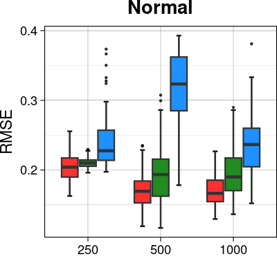
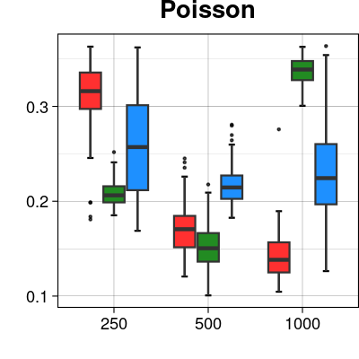
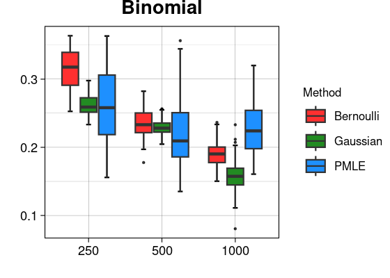
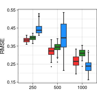
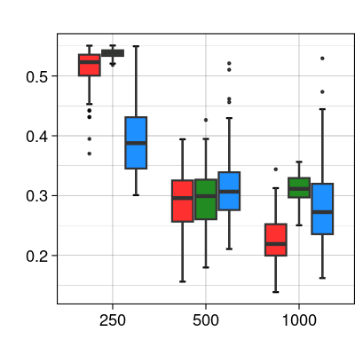
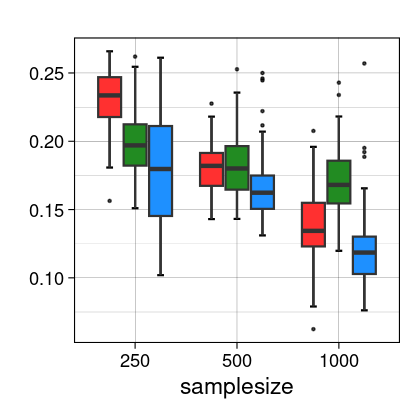
Figure 1: Boxplots of RMSEs for dispersion parameters of Gaussian data (left column), Poisson data (middle column) and binomial data (right column) across Scenarios 1 (top row), 2 (middle row) and 3 (bottom row). Outliers in the dispersion were cut at the $95$-th percentile.

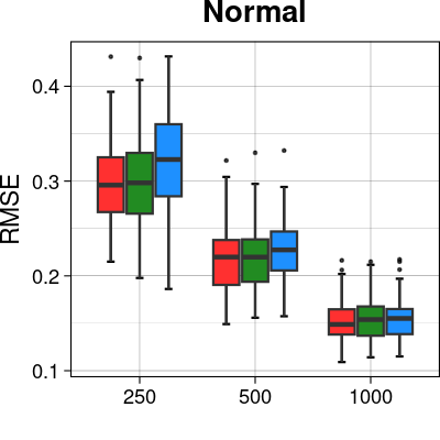
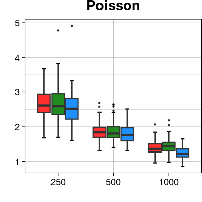
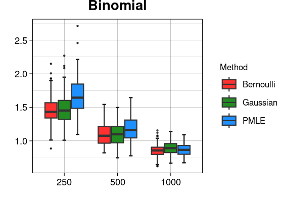
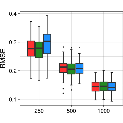
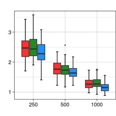
Figure 5: Boxplots of RMSEs for mean estimates of normal data (left column), Poisson data (middle column) and binomial data (right column) across Scenarios 1 (top row), 2 (middle row) and 3 (bottom row).

Figure 1 presents boxplots for the RMSEs of the dispersion estimates for the three distributions and across all different scenarios. Figure 5 in Appendix E contains the respective boxplots for the mean estimates. All three methods estimate the mean very well. Figure 1 reveals that dropout regularization is competitive with PMLE in all scenarios.

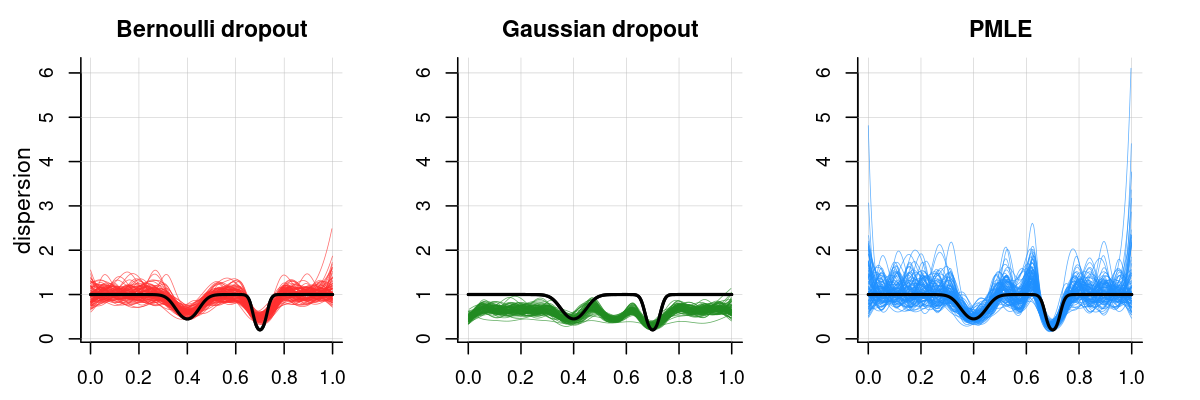
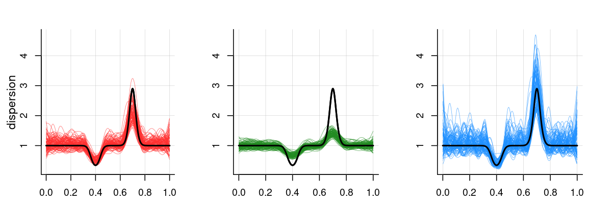
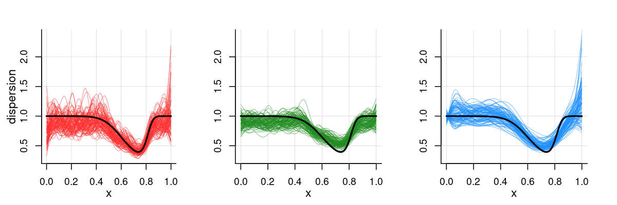
Figure 8: Estimated dispersion effects in the Poisson model for Bernoulli dropout (left), Gaussian dropout (middle) and PMLE (right) in Scenario 1 (upper row), Scenario 2 (middle row) and Scenario 3 (bottom row) for $R=100$ replicates of size $n=1000$. The true effects are given by the black lines.

In Scenario 1 with Gaussian data, dropout outperforms PMLE across all sample sizes, and Bernoulli dropout performs slightly better than Gaussian dropout. With count data the difference between dropout and PMLE is less pronounced. Performance of Gaussian dropout is poor for Poisson data in Scenarios 1 and 2 for the largest sample size, $n=1000$. Figure 8 gives evidence that this poor performance is associated with large bias in estimation of the dispersion function. However, Gaussian dropout performs slightly better than Bernoulli dropout in most cases involving count data. In the binomial case, dropout shows improved performance relative to PMLE as the sample size increases.

Scenario 2 is based on rare but important features as well, but now for some values of the covariate there is strong underdispersion. We find that in small sample sizes dropout performs well compared to dropout for Gaussian and binomial data, but poorly for Poisson data. In other cases the differences are minor. For Gaussian data, Bernoulli dropout is slightly better than Gaussian dropout, similar to Scenario 1.

Since the true dispersion function for Scenario 3 cannot be modeled through rare features, dropout performs slightly worse than PMLE across all distributions and sample sizes for this case. The findings with respect to the three scenarios match our theoretical analysis from Section 3.

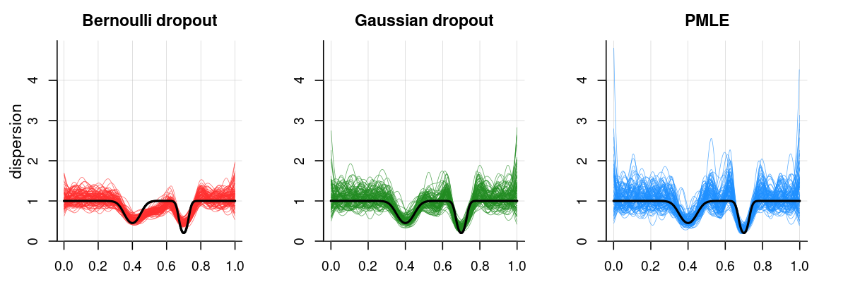
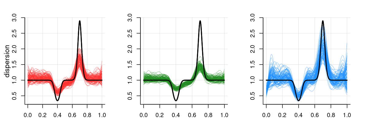
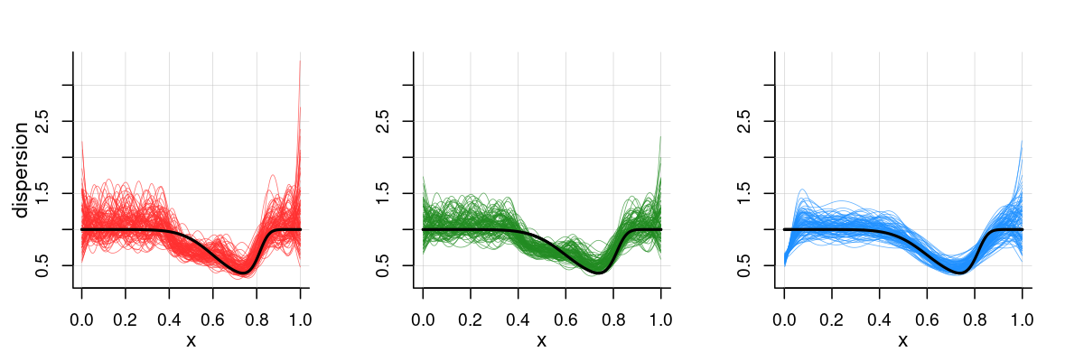
Figure 2: Estimated dispersion effects in the Gaussian model for Bernoulli dropout (left), Gaussian dropout (middle) and PMLE (right) in Scenario 1 (upper row), Scenario 2 (middle row) and Scenario 3 (bottom row) for $R=100$ replicates of size $n=1000$. The true effects are given by the black lines.

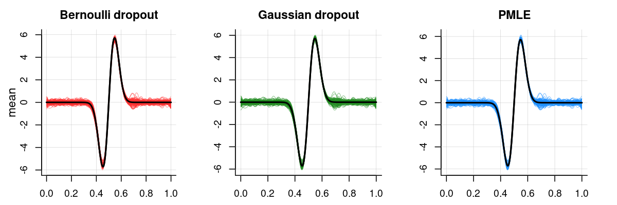
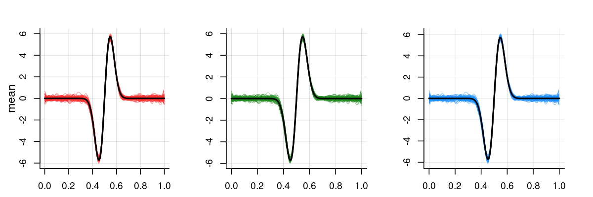
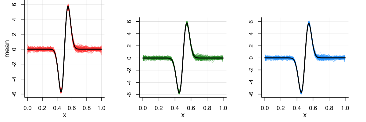
Figure 6: Estimated mean effects in the normal model for Bernoulli dropout (left), Gaussian dropout (middle) and PMLE (right) in Scenario 1 (upper row), Scenario 2 (middle row) and Scenario 3 (bottom row) for $R=100$ replicates of size $n=1000$. The true effects are given by the black lines.

Figure 2 depicts the estimated dispersion effects from Gaussian data for all three scenarios and $n=1000$. Figure 6 in Appendix E contains the same plots for the mean estimates. The estimation of the mean function is quite accurate across the three methods. The estimated dispersion functions are less accurate. Since accurate variance estimation can only occur when the mean is well-estimated, estimating the dispersion function is more difficult (Gijbels et al., 2010). However, in most cases the dispersion estimates reproduced the correct shape. The PMLE estimates suffer from oscillations at the boundaries. For Scenario 2, the rapid changes are not captured very well by Gaussian dropout, particularly where they correspond to regions of underdispersion. The problem also occurs with Bernoulli dropout but is less pronounced. For Scenario 3 the dropout estimates of the dispersion function are noticeably less smooth than the estimates obtained via PMLE. This is consistent with the boxplots at the bottom of the first column of Figure 1.

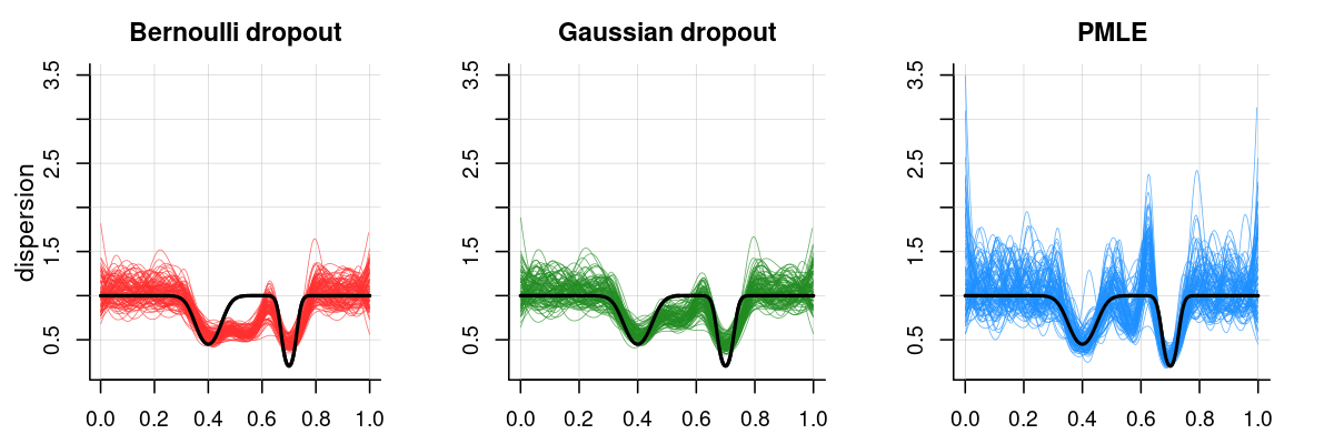
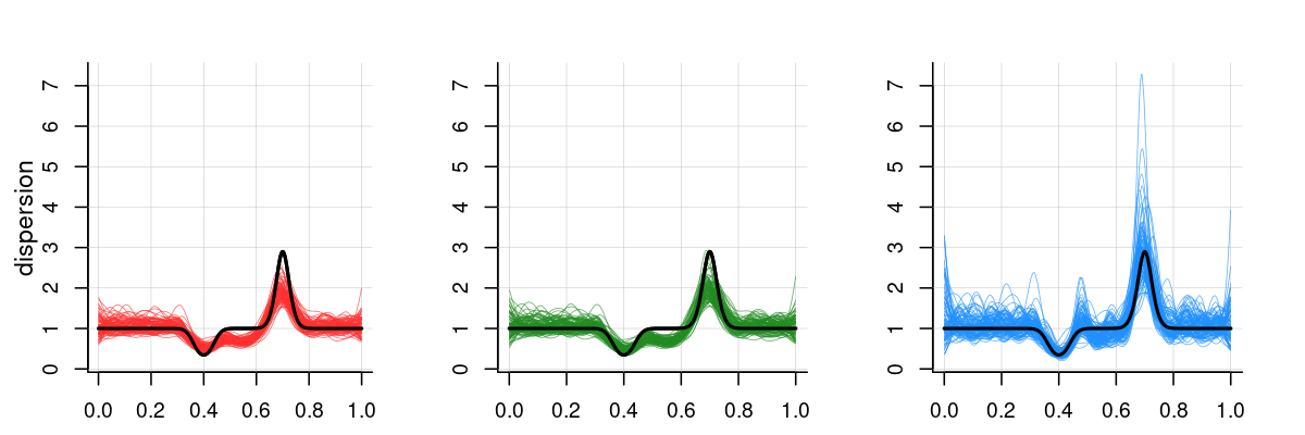
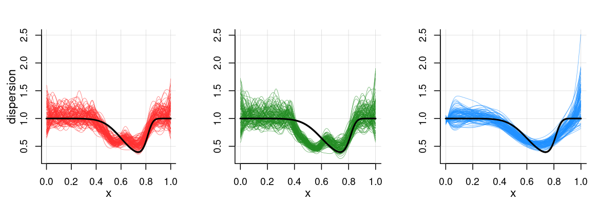
Figure 3: Estimated dispersion effects in the binomial model for Bernoulli dropout (left), Gaussian dropout (middle) and PMLE (right) in Scenario 1 (upper row), Sscenario 2 (middle row) and Scenario 3 (bottom row) for $R=100$ replicates of size $n=1000$. The true effects are given by the black lines.

Figure 3 presents the estimated dispersion effects obtained from binomial data. Previous observations with respect to Gaussian data apply as well. Additionally, we can observe a notable local minimum in the dispersion estimates in the vicinity of $x\approx 0.5$. This is even more pronounced in case of smaller sample sizes (not shown). It confirms the observation from Section 3, that there is an incentive to compensate a large variance caused by the mean with overdispersion. The variance function of the binomial distribution is given by $V(\mu)=\mu(N-\mu)/N$, i.e. its maximizer is $N/2$. Thus, one can expect this behavior to take place at $x\approx 0.5$ for the mean function depicted in Figure A.1. For the Poisson distribution, the variance function is given by $\mathbb{V}(\mu)=\mu$, and again referring to Figure A.1, we expect the regularization to favour overdispersion around $x\approx 0.55$. This could be the reason for the reduced competitiveness of dropout regularization in the case of count data. The PMLE estimates are less smooth than the dropout estimates in Scenarios 1 and 2 and they oversmooth the true function in Scenario 3.

5 Conclusion

We studied dropout regularization in the context of flexible GLMs based on the DEF. Our theoretical analysis shows that dropout favors rare but important features in the mean and dispersion parameters, and overdispersion relative to underdispersion. Overdispersion alleviates the penalization on the mean provided the dispersion can be modelled by rare but important features itself. These findings are further justified by an empirical application to adaptive smoothing with B-splines. Our experiments confirm that dropout regularization outperforms PMLE under ideal conditions. Deviations from the ideal scenario, such as the presence of underdispersion or a mean or dispersion function which cannot be modelled by rare but important features, leads to a decrease in performance of dropout regularization relative to PMLE. In future research these findings could be extended to generalized additive models and quasi-likelihood estimation. Our findings extend previous work on dropout regularization for GLMs and add to the theoretical understanding of dropout methods in general.

Appendix A Transformation of the dropout objective

Recall that $\mathbb{E}[\bm{x}_{i}^{T}(\bm{\beta}\odot\bm{\xi}_{i})]=\bm{x}_{i}^{T}\bm{\beta}$. Writing $\mathbb{E}[b(\bm{x}_{i}^{T}(\bm{\beta}\odot\bm{\xi}_{i}))]=\mathbb{E}[b(\bm{x}_{i}^{T}(\bm{\beta}\odot\bm{\xi}_{i}))]+b(\bm{x}_{i}^{T}\bm{\beta})-b(\bm{x}_{i}^{T}\bm{\beta})$ the objective in (4) is

$$\min_{\bm{\beta},\bm{\alpha}}\left\{-\sum_{i=1}^{n}\ell_{i}(\bm{\beta},\bm{\alpha})+\sum_{i=1}^{n}\gamma_{i}\frac{\left\{\mathbb{E}[b(\bm{x}_{i}^{T}(\bm{\beta}\odot\bm{\xi}_{i}))]-b(\bm{x}_{i}^{T}\bm{\beta})\right\}}{\phi/\nu_{i}}\right\}$$ (15)

This shows that the original dropout objective is the maximum likelihood objective for $\bm{\beta}$ and $\bm{\alpha}$ plus a penalization term. The penalization term in (15) does not depend on the responses $y_{i}$ and therefore does not penalize the accuracy. The convexity of $b$ together with Jensen’s inequality imply that

$$\mathbb{E}[b(\bm{x}_{i}^{T}(\bm{\beta}\odot\bm{\xi}_{i}))]-b(\bm{x}_{i}^{T}\bm{\beta})\geqslant 0,$$ (16)

i.e. nonnegativity of the penalty.

Given some random variable $X$ and a measurable function $f$, we can approximate $\mathbb{E}[f(X)]$ using a second order Taylor approximation of $f$ around $\mu_{X}:=\mathbb{E}[X]$:

$$\mathbb{E}[f(X)]\approx f(\mu_{X})+f^{\prime}(\mu_{X})\mathbb{E}[X-\mu_{X}]+\frac{1}{2}f^{\prime\prime}(\mu_{X})\mathbb{E}[X-\mu_{X}]^{2}$$

Using such an approximation for $\mathbb{E}[b(\bm{x}_{i}^{T}(\bm{\beta}\odot\bm{\xi}_{i}))]$ gives $\mathbb{E}[b(\bm{x}_{i}^{T}(\bm{\beta}\odot\bm{\xi}_{i}))]-b(\bm{x}_{i}^{T}\bm{\beta})\approx b^{\prime\prime}(\bm{x}_{i}^{T}\bm{\beta})\mathbb{V}[\bm{x}_{i}^{T}(\bm{\beta}\odot\bm{\xi}_{i})]/2$. Plugging it into the penalty gives

$$\frac{1}{2}\sum_{i=1}^{n}\gamma_{i}b^{\prime\prime}(\bm{x}_{i}^{T}\bm{\beta})\mathbb{V}[\bm{x}_{i}^{T}(\bm{\beta}\odot\bm{\xi}_{i})]=\frac{1}{2}\sigma^{2}_{\mu}\bm{\beta}^{T}\text{diag}(\bm{X}^{T}\bm{W}\bm{X})\bm{\beta},$$ (17)

where $\bm{X}\in\mathbb{R}^{n,d_{\mu}}$ is the design matrix of the mean and the diagonal weight matrix $\bm{W}$ depends on both $\bm{\beta}$ and $\bm{\alpha}$ and is given by

$$\bm{W}:=\text{diag}\left(\frac{\gamma_{1}b^{\prime\prime}(\bm{x}_{1}^{T}\bm{\beta})}{\phi/\nu_{1}},\ldots,\frac{\gamma_{n}b^{\prime\prime}(\bm{x}_{n}^{T}\bm{\beta})}{\phi/\nu_{n}}\right)\in\mathbb{R}^{n,n}.$$

Since $b$ is convex, $b^{\prime\prime}>0$, and since $\gamma_{i}$ is nonnegative the weight matrix $\bm{W}$ is positive definite. The same holds true for $\text{diag}(\bm{X}^{T}\bm{W}\bm{X})$. Substituting the right-hand side of (17) into (15) shows that (6) approximates (4).

Appendix B Fisher information

Given some log-likelihood $\ell:\Theta\rightarrow\mathbb{R}$, the Fisher information is defined by $\mathcal{I}(\theta):=\mathbb{E}_{\theta}[\ell^{\prime}(\theta)\ell^{\prime}(\theta)^{T}]$. Under certain regularity conditions (see Proposition 3.1 in Shao (2003)) the so-called information equality

$$\mathcal{I}(\theta)=-\mathbb{E}_{\theta}[\ell^{\prime\prime}(\theta)]$$

holds, where $\ell^{\prime\prime}(\theta)=H(\ell)$ with $H(\ell)$ is the Hessian of the log-likelihood $\ell$. Our statistical model is a product model $(\mathcal{Y}^{n},\mathcal{F}^{\otimes n},(\mathbb{P}^{\otimes n}_{\theta})_{\theta\in\Theta})$, which fulfills these regularity conditions. From the approximated log-likelihood

$$\ell(\bm{\beta},\bm{\alpha})=\frac{1}{2}\bm{z}^{T}\bm{\alpha}+\exp(\bm{z}^{T}\bm{\alpha})\frac{y\bm{x}^{T}\bm{\beta}-b(\bm{x}^{T}\bm{\beta})}{\phi/\nu}+(1-\exp(\bm{z}^{T}\bm{\alpha}))\frac{y\theta(y)-b(\theta(y))}{\phi/\nu}$$

we first calculate the first derivatives with respect to $\bm{\beta}$ and $\bm{\alpha}$:

$$\frac{\partial\ell}{\partial\bm{\beta}}(\bm{\beta},\bm{\alpha}) =\bm{x}^{T}\left\{\frac{\exp(\bm{z}^{T}\bm{\alpha})}{\phi/\nu}(y-b^{\prime}(\bm{x}^{T}\bm{\beta}))\right\}$$

$$\frac{\partial\ell}{\partial\bm{\alpha}}(\bm{\beta},\bm{\alpha}) =\bm{z}^{T}\left\{\frac{1}{2}+\frac{\exp(\bm{z}^{T}\bm{\alpha})}{\phi/\nu}(y\bm{x}^{T}\bm{\beta}-b(\bm{x}^{T}\bm{\beta})-(y\theta(y)-b(\theta(y))))\right\}$$

We then proceed to compute all second derivatives:

$$\frac{\partial\ell}{\partial\bm{\beta}\partial\bm{\beta}^{T}}(\bm{\beta},\bm{\alpha}) =-\bm{x}^{T}\bm{x}\left\{\frac{\exp(\bm{z}^{T}\bm{\alpha})}{\phi/\nu}b^{\prime\prime}(\bm{x}^{T}\bm{\beta})\right\}$$

$$\frac{\partial\ell}{\partial\bm{\beta}\partial\bm{\alpha}^{T}}(\bm{\beta},\bm{\alpha}) =\bm{x}^{T}\bm{z}\left\{\frac{\exp(\bm{z}^{T}\bm{\alpha})}{\phi/\nu}(y-b^{\prime}(\bm{x}^{T}\bm{\beta}))\right\}$$

$$\frac{\partial\ell}{\partial\bm{\alpha}\partial\bm{\alpha}^{T}}(\bm{\beta},\bm{\alpha}) =\bm{z}^{T}\bm{z}\left\{\frac{\exp(\bm{z}^{T}\bm{\alpha})}{\phi/\nu}(y\bm{x}^{T}\bm{\beta}-b(\bm{x}^{T}\bm{\beta})-(y\theta(y)-b(\theta(y))))\right\}$$

$$\frac{\partial\ell}{\partial\bm{\alpha}\partial\bm{\beta}^{T}}(\bm{\beta},\bm{\alpha}) =\bm{z}^{T}\bm{x}\left\{\frac{\exp(\bm{z}^{T}\bm{\alpha})}{\phi/\nu}(y-b^{\prime}(\bm{x}^{T}\bm{\beta}))\right\}$$

Assuming that the linear parametric assumption holds, i.e. $\mathbb{E}[Y]=b^{\prime}(\bm{x}^{T}\bm{\beta})$ for some true parameter value $\bm{\beta}$, we obtain

$$\mathcal{I}(\bm{\beta},\bm{\alpha})=\begin{bmatrix}\mathcal{I}(\bm{\beta})&\bm{0}\\ \bm{0}&\mathcal{I}(\bm{\alpha})\end{bmatrix}=\begin{bmatrix}w_{\bm{\beta}}(\bm{x},\bm{z})\bm{x}^{T}\bm{x}&\bm{0}\\ \bm{0}&w_{\bm{\alpha}}(\bm{x},\bm{z})\bm{z}^{T}\bm{z}\end{bmatrix},$$

where the weights $w_{\bm{\beta}}(\bm{x},\bm{z})$ and $w_{\bm{\alpha}}(\bm{x},\bm{z})$ of the respective blocks are given by

$$w_{\bm{\beta}}(\bm{x},\bm{z}) :=\left\{\frac{\exp(\bm{z}^{T}\bm{\alpha})}{\phi/\nu}b^{\prime\prime}(\bm{x}^{T}\bm{\beta})\right\},$$

$$w_{\bm{\alpha}}(\bm{x},\bm{z}) :=\left\{\frac{\exp(\bm{z}^{T}\bm{\alpha})}{\phi/\nu}(b(\bm{x}^{T}\bm{\beta})-b^{\prime}(\bm{x}^{T}\bm{\beta})\bm{x}^{T}\bm{\beta}+\mathbb{E}[Y\theta(Y)]-\mathbb{E}[b(\theta(Y))])\right\}.$$

The term $w_{\bm{\alpha}}(\bm{x},\bm{z})$ is approximately $1$. To see this, observe that $w_{\bm{\alpha}}(\bm{x},\bm{z})$ is $\exp(\bm{z}^{T}\bm{\alpha})$ times the expected deviance for the exponential family used in constructing the DEF. Equation (2.15) in Efron (1986) implies that the expected deviance is $1/\gamma=\exp(-\bm{z}^{T}\bm{\alpha})$ in a certain limiting regime, giving $w_{\bm{\alpha}}(\bm{x},\bm{z})\approx 1$. The observed Fisher information $\widehat{\mathcal{I}}(\bm{\beta})$ is an estimator of the Fisher information $\mathcal{I}(\bm{\beta})$ and it is given by

$$\widehat{\mathcal{I}}(\bm{\beta}):=\frac{1}{n}\sum_{i=1}^{n}-\frac{\partial\ell_{i}}{\partial\bm{\beta}\partial\bm{\beta}^{T}}(\bm{\beta},\bm{\alpha})=\frac{1}{n}\sum_{i=1}^{n}w_{\bm{\beta}}(\bm{x}_{i},\bm{z}_{i})\bm{x}_{i}^{T}\bm{x}_{i}=\frac{1}{n}\bm{X}^{T}\bm{W}\bm{X},$$

showing that $\bm{\Theta}=\text{diag}(n\widehat{\mathcal{I}}(\bm{\beta}))^{1/2}$. With $w_{\bm{\alpha}}(\bm{x},\bm{z})\approx 1$ we obtain analogously

$$\widehat{\mathcal{I}}(\bm{\alpha}):=\frac{1}{n}\sum_{i=1}^{n}-\frac{\partial\ell_{i}}{\partial\bm{\alpha}\partial\bm{\alpha}^{T}}(\bm{\beta},\bm{\alpha})=\frac{1}{n}\sum_{i=1}^{n}w_{\bm{\alpha}}(\bm{x}_{i},\bm{z}_{i})\bm{z}_{i}^{T}\bm{z}_{i}\approx\frac{1}{n}\bm{Z}^{T}\bm{Z},$$

such that $\bm{\Gamma}\approx\text{diag}(n\widehat{\mathcal{I}}(\bm{\alpha}))^{1/2}$.

Appendix C Details on the SGD algorithm

We use SGD to estimate the parameters $\bm{\beta}$ and $\bm{\alpha}$ which parameterize the linear predictors $\theta_{i}(x)=\bm{B}_{\mu}(x)^{T}\bm{\beta}$ and $\log(\gamma_{i}(x))=\bm{B}_{\gamma}(x)^{T}\bm{\alpha}$, where $\bm{B}_{\mu}(x)$ and $\bm{B}_{\gamma}(x)$ are vectors of all evaluated B-spline basis functions at $x\in[a,b]$. For given hyperparameters $\sigma^{2}_{\mu}$ and $\sigma^{2}_{\gamma}$ and after setting initial parameter values $\bm{\beta}^{(0)}$ and $\bm{\alpha}^{(0)}$ the estimation procedure starts performing SGD-updates on both parameter vectors. At every iteration $i$, for given estimates $\bm{\beta}^{(i-1)}$ and $\bm{\alpha}^{(i-1)}$ it performs the updates

$$\bm{\beta}^{(i)} =\bm{\beta}^{(i-1)}+\eta^{(i)}_{\mu}s^{(i)}(\bm{\beta}^{(i-1)}),$$

$$\bm{\alpha}^{(i)} =\bm{\alpha}^{(i-1)}+\eta^{(i)}_{\gamma}s^{(i)}(\bm{\alpha}^{(i-1)}).$$

The scores $s^{(i)}(\bm{\beta}^{(i-1)})$ and $s^{(i)}(\bm{\alpha}^{(i-1)})$ are estimates based on a batch sample, which is perturbed by Gaussian or Bernoulli dropout noise. The batch sample is obtained by sampling $b=30$ indices uniformly from the index set $\{1,\ldots,n\}$. The learning rates $\eta^{(i)}_{\mu}$ and $\eta^{(i)}_{\gamma}$ are determined by ADADELTA with default values suggested in (Zeiler, 2012). The procedure terminates if a maximum number of iterations has been performed or if the log-likelihood reaches a stationary point.

We perform random search $k$-fold CV in order to select $\sigma_{\mu}$ and $\sigma_{\gamma}$ from the hyperparameter space $\mathcal{H}\subseteq\mathbb{R}_{+}^{2}$ optimally. That is, after creating $k\in\mathbb{N}$ folds from the data $\{\bm{y},\bm{B}_{\mu},\bm{B}_{\gamma}\}$ we draw $s\in\mathbb{N}$ samples $\{(\sigma_{\bm{\xi},1},\sigma_{\bm{\zeta},1}),\ldots,(\sigma_{\bm{\xi},s},\sigma_{\bm{\zeta},s})\}$ from the uniform distribution over $\mathcal{H}$. Then, for each tuple $(\sigma_{\bm{\xi},j},\sigma_{\bm{\zeta},j})$ and $j=1,\ldots,s$ we estimate the model $k$ times. Each of these $k$ estimates will be based on all but one fold. The left-out fold is used to evaluate each estimated model by calculating the log-likelihood. The average over the $k$ log-likelihood values corresponding to the $j$-th sample is given by $\ell_{j}$. The optimal smoothing parameters $\sigma_{\mu}^{*}$ and $\sigma_{\gamma}^{*}$ are set according to

$$(\sigma_{\mu}^{*},\sigma_{\gamma}^{*})\,\leftarrow\,(\sigma_{\bm{\xi},j^{*}},\sigma_{\bm{\zeta},j^{*}}),$$

where the index $j^{*}$ is defined as $j^{*}=\operatorname*{arg\,max}_{j\in\{1,\ldots,s\}}\{\ell_{1},\ldots,\ell_{s}\}$.

The code is publicly available through Github. It relies on parallel computing and all computations were performed on a GPU with 192 GB memory and 12 physical cores at 3.0 GHz. It also contains the code from Gijbels et al. (2010) obtained via an URL provided in their publication.

Appendix D Details on the simulation design

Testfunctions

As mentioned before, dropout favors rare but important features. The true mean and dispersion function from which we simulate data should therefore allow for this characteristic, in view of the chosen functional basis. We use B-splines with a relatively large number of knots, such that the basis functions are only supported on small compact sets of the domain. If the true function to be approximated with these basis functions is mostly flat, but spikes on small subsets of the domain, then we have correctly chosen a basis of rare but important features. All testfunctions were constructed with this idea in mind, as can be seen in Figure 4. This includes the intentional choice $g_{2}$ in order to verify if dropout regularization deteriorates in this case.

The testfunctions for the mean are

$$f_{1} :[0,1]\rightarrow\mathbb{R},\quad x\mapsto 2\sin(4\pi x)\phi_{0.5,0.05^{2}}(x),$$ (18)

$$f_{2} :[0,1]\rightarrow\mathbb{R},\quad x\mapsto 40+10\sin(4\pi x)\phi_{0.5,0.05^{2}}(x),$$ (19)

whereas $f_{1}$ was used to simulate normal data and $f_{2}$ served as mean function in the Poisson and binomial case. We will fix the number of trials to $N=70$ when using $f_{3}$ to model double binomial data. The function $\phi_{\mu,\sigma^{2}}$ is the PDF of the normal distribution $\mathcal{N}(\mu,\sigma^{2})$. For each distribution, we combined the mean function with one of the three dispersion functions

$$g_{1} :[0,1]\rightarrow\mathbb{R},\quad x\mapsto\exp\{-0.08\phi_{0.4,0.04^{2}}(x)-0.08\phi_{0.7,0.02^{2}}(x)\},$$ (20)

$$g_{2} :[0,1]\rightarrow\mathbb{R},\quad x\mapsto\exp\{-0.08\phi_{0.4,0.03^{2}}(x)+0.08\phi_{0.7,0.03^{2}}(x)\},$$ (21)

$$g_{3} :[0,1]\rightarrow\mathbb{R},\quad x\mapsto\exp\left\{\frac{2}{0.15}\phi_{0,1}\left(\frac{x-0.8}{0.15}\right)\Phi_{0,1}\left(-4\left(\frac{x-0.8}{0.15}\right)\right)\right\}.$$ (22)

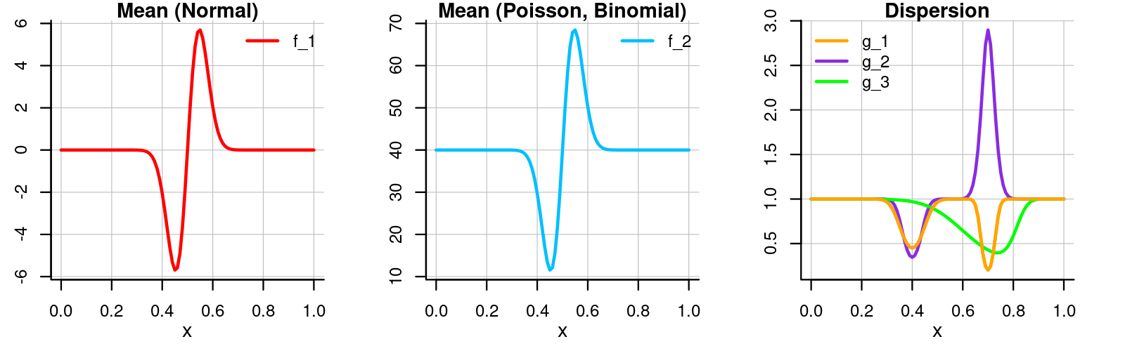
Figure 4: Testfunctions for the mean and dispersion.

Simulation design

For a fixed distribution $\mathbb{P}\in\{\mathcal{N},\text{DPoi},\text{DBin}\}$, mean function $f_{i}$ with $i\in\{1,2\}$, dispersion function $g_{j}$ with $j\in\{1,2,3\}$ and for a sample size of $n=250,500,1000$, the simulation procedure consists of the following steps:

1. Simulate $R+1$ with $R=100$ data sets $\mathcal{D}(\mathbb{P},i,j,n)[m]=\{(y_{k},x_{k})\}_{k=1}^{n}$ for $m=1,\ldots,R+1$, i.e. we denote by $\mathcal{D}(\mathbb{P},i,j,n)[m]$ the $m$-th data set of sample size $n$ which was simulated from the distribution $\mathbb{P}$ with mean $f_{i}$, dispersion $g_{j}$. The values $x_{k}$ were sampled from $\mathcal{U}([0,1])$. Each dependent variable $y_{k}$ was then sampled from the respective $\text{DEF}(\gamma_{k},\mu_{k},\phi)$ with $\gamma_{k}=g_{j}(x_{k})$ and $\mu_{k}=f_{i}(x_{k})$. We fixed $\sigma^{2}=0.8^{2}$ in the normal case.

2. Perform $k$-fold likelihood cross-validation for $k=5$ on the first replicate $\mathcal{D}(\mathbb{P},i,j,n)[1]$ for each regularization method, where the number of drawn samples from the uniform distribution over $\mathcal{H}$ is fixed to $s=500$:

   1. For Bernoulli dropout fix $\mathcal{H}=\mathcal{I}_{\mu}\times\mathcal{I}_{\gamma}=[0,1]^{2}$.

   2. For Gaussian dropout fix $\mathcal{H}=\mathcal{I}_{\mu}\times\mathcal{I}_{\gamma}=[0,3]\times[0,6]$.

   3. For PMLE fix $\mathcal{H}=\mathcal{I}_{\mu}\times\mathcal{I}_{\gamma}=[0,15000]^{2}$.

3. Use the optimal smoothing parameters for each method obtained in (2) to estimate for the remaining $R$ data sets $\mathcal{D}(\mathbb{P},i,j,n)[m]$ with $m=2,\ldots,R+1$ the corresponding models $\mathcal{M}(\mathbb{P},i,j,n,\mathcal{R})[m]$. By $\mathcal{M}(\mathbb{P},i,j,n,\mathcal{R})[m]$ we denote the model estimate obtained from data set $\mathcal{D}(\mathbb{P},i,j,n)[m]$ and regularization method $\mathcal{R}\in\{\texttt{bernoulli},\texttt{gaussian},\texttt{pmle}\}$. We will simply write $\mathcal{M}(\mathbb{P},i,j,n,\mathcal{R})$ in order to refer to all estimates. Out of convenience, we will sometimes drop $n$ and $R$ and only write $\mathcal{M}(\mathbb{P},i,j)$ when we want to refer to all models which have $\mathbb{P}$, $i$ and $j$ in common, but vary across $n$ and $\mathcal{R}$.

4. Let $\widehat{\pi}^{(m)}$ be the mean or dispersion estimate obtained from $\mathcal{D}(\mathbb{P},i,j,n)[m]$ and $\pi$ its ground truth counterpart. To evaluate the performance of the three competing regularization methods we compute the RMSE

   $$\text{RMSE}(\widehat{\pi}^{(m)},\pi):=\left(\sum_{x\in\Pi}\left(\widehat{\pi}^{(m)}(x)-\pi(x)\right)^{2}\right)^{1/2}$$ (23)

   for all $m=2,\ldots,R+1$ and an equidistant grid $\Pi:=[0,1/\kappa,2/\kappa,\ldots,1]$ of length $\kappa+1$ with $\kappa=500$.

We employ natural cubic B-splines bases based on $m_{\mu}=30$ equidistant knots in the mean and $m_{\gamma}=20$ equidistant knots in the dispersion model.

Appendix E Additional plots

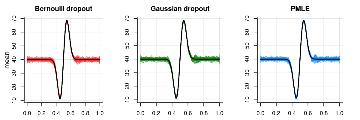
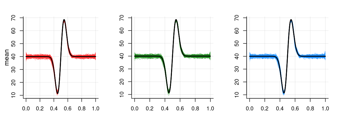
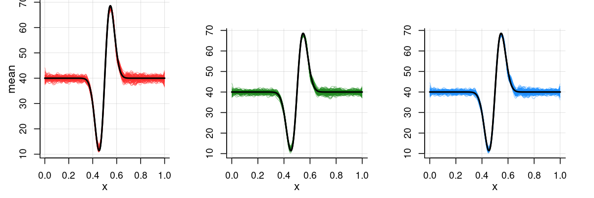
Figure 7: Estimated mean effects in the binomial model for Bernoulli dropout (left), Gaussian dropout (middle) and PMLE (right) in Scenario 1 (upper row), Scenario 2 (middle row) and Scenario 3 (bottom row) for $R=100$ replicates of size $n=1000$. The true effects are given by the black lines.

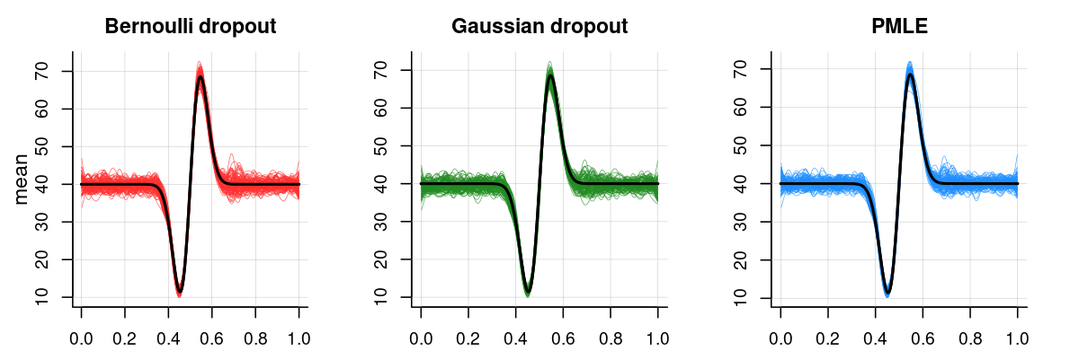
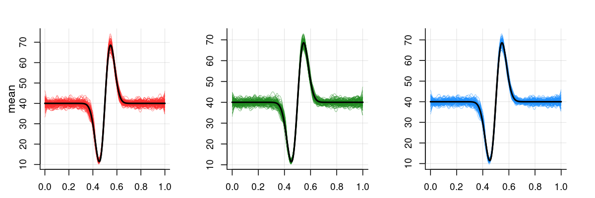
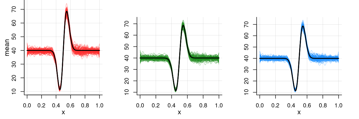
Figure 9: Estimated mean effects in the Poisson model for Bernoulli dropout (left), Gaussian dropout (middle) and PMLE (right) in Scenario 1 (upper row), Scenario 2 (middle row) and Scenario 3 (bottom row) for $R=100$ replicates of size $n=1000$. The true effects are given by the black lines.

References

- (1)
- Baldi and Sadowski (2013) Baldi, P. and Sadowski, P. J. (2013). Understanding dropout, Advances in neural information processing systems 26.
- Bishop (1995) Bishop, C. M. (1995). Training with noise is equivalent to tikhonov regularization, Neural Computation 7(1): 108–116.
- Burges and Schölkopf (1996) Burges, C. J. and Schölkopf, B. (1996). Improving the accuracy and speed of support vector machines, Advances in neural information processing systems 9.
- Dunn and Smyth (2018) Dunn, P. K. and Smyth, G. K. (2018). Generalized Linear Models With Examples in R, Springer Texts in Statistics, first edition edn, Springer New York.
- Efron (1986) Efron, B. (1986). Double exponential families and their use in generalized linear regression, Journal of the American Statistical Association 81(395): 709–721.
- Eilers and Marx (1996) Eilers, P. H. C. and Marx, B. D. (1996). Flexible smoothing with b-splines and penalties, Statistical Science 11(2): 89–121.
- Gijbels et al. (2010) Gijbels, I., Prosdocimi, I. and Claeskens, G. (2010). Nonparametric estimation of mean and dispersion functions in extended generalized linear models, TEST 19(3): 580–608.
- Helmbold and Long (2015) Helmbold, D. P. and Long, P. M. (2015). On the inductive bias of dropout, Journal of Machine Learning Research 16(105): 3403–3454.
- Hinton et al. (2012) Hinton, G. E., Srivastava, N., Krizhevsky, A., Sutskever, I. and Salakhutdinov, R. R. (2012). Improving neural networks by preventing co-adaptation of feature detectors, arXiv: 1207.0580.
- Lee and Nelder (2000) Lee, Y. and Nelder, J. A. (2000). The relationship between double-exponential families and extended quasi-likelihood families, with application to modelling geissler’s human sex ratio data, Journal of the Royal Statistical Society. Series C 49(3): 413–419.
- Lehmann and Casella (1998) Lehmann, E. L. and Casella, G. (1998). Theory of Point Estimation, Springer texts in statistics, second edition edn, Springer.
- Maaten et al. (2013) Maaten, L., Chen, M., Tyree, S. and Weinberger, K. (2013). Learning with marginalized corrupted features, International Conference on Machine Learning, PMLR, pp. 410–418.
- McCullagh and Nelder (1998) McCullagh, P. and Nelder, J. A. (1998). Generalized Linear Models, number 37 in Monographs on Statistics and Applied Probability, second edition edn, Chapman & Hall/CRC.
- Merity et al. (2017) Merity, S., Keskar, N. S. and Socher, R. (2017). Regularizing and optimizing lstm language models, arXiv:1708.02182.
- Shao (2003) Shao, J. (2003). Mathematical Statistics, Springer texts in statistics, second edition edn, Springer.
- Srivastava et al. (2014) Srivastava, N., Hinton, G., Krizhevsky, A., Sutskever, I. and Salakhutdinov, R. (2014). Dropout: A simple way to prevent neural networks from overfitting, Journal of Machine Learning Research 15(56): 1929–1958.
- Tan and Le (2019) Tan, M. and Le, Q. (2019). EfficientNet: Rethinking model scaling for convolutional neural networks, Proceedings of the 36th International Conference on Machine Learning, PMLR, pp. 6105–6114.
- Van Erven et al. (2014) Van Erven, T., Kotłowski, W. and Warmuth, M. K. (2014). Follow the leader with dropout perturbations, Proceedings of The 27th Conference on Learning Theory, Vol. 35, PMLR, Barcelona, Spain, pp. 949–974.
- Wager et al. (2013) Wager, S., Wang, S. and Liang, P. S. (2013). Dropout training as adaptive regularization, Advances in neural information processing systems 26.
- Wang and Manning (2013) Wang, S. and Manning, C. (2013). Fast dropout training, international conference on machine learning, PMLR, pp. 118–126.
- Wei et al. (2020) Wei, C., Kakade, S. and Ma, T. (2020). The implicit and explicit regularization effects of dropout, International conference on machine learning, PMLR, pp. 10181–10192.
- Zeiler (2012) Zeiler, M. D. (2012). ADADELTA: An adaptive learning rate method, arXiv:1212.5701.