Input Distribution Optimization in OFDM Dual-Function Radar-Communication Systems

Abstract

Orthogonal frequency division multiplexing (OFDM) has been widely adopted in dual-function radar-communication (DFRC) systems, where radar and communications are performed simultaneously with a common signal. However, with random communication symbols (CS) in DFRC, the transmit signal has a random ambiguity function that affects the radar’s range-velocity estimation performance, whose influence is remained uncovered. Hence, this paper focuses on minimizing the outlier probability (OP) – the probability of incorrectly estimating a target’s range-velocity bin – in OFDM DFRC w.r.t the CS probability distribution (i.e., the input distribution). Conditioned on the CSs, the OP only depends on the CS magnitudes. Hence, we consider the following two schemes for the above optimization: CSs with (1) constant magnitude (phase shift keying input), and (2) random magnitude (Gaussian input). For (1), the problem reduces to the familiar power allocation design across OFDM’s subcarriers and symbols, with uniform power allocation across subcarriers and a windowed power allocation across symbols being near-optimal. For (2), the mean and variance of the Gaussian distribution at each subcarrier is optimized, with an additional communication constraint to avoid the zero-variance solution where no CSs are carried. We observe that subcarriers with strong communication channels feature strong variance (i.e., favour communications) while the others are characterized by a strong mean (favouring radar). However, the overall power allocation (i.e., the sum of mean and variance) across the OFDM subcarriers and symbols is similar to (1). Simulations show that CSs with random magnitudes degrade the sensing performance, but can be compensated significantly with the proposed input distribution optimization, which highlights the importance of considering the effect of CSs’ random magnitudes on DFRC signal design.

I Introduction

Dual-function radar-communication (DFRC) has attracted considerable interest as a solution to the problem of spectrum shortage arising from the increasing use of wireless technologies [paul2016survey, 8999605]. In DFRC, a common signal is used for radar and communications simultaneously [9737357, 9705498]. Hence, of vital significance in DFRC systems is the choice and design of a suitable signal that performs both communications and radar satisfyingly [hwang2008ofdm, sturm2011waveform].

The orthogonal frequency division multiplexing (OFDM) signal is a strong candidate for DFRC systems given its benefits for both communications and radar. For the former, OFDM is well-known to provide robustness against channel fading and combat inter-symbol interference to realize higher data rates [hwang2008ofdm]. For the latter, a highly efficient 2D-FFT (2-dimensional fast Fourier transform) based range-velocity bin estimator exists and has been shown to achieve very promising estimation accuracy [sturm2011waveform, 8805161, berger2010signal].

The performance of OFDM for communication and radar in DFRC can be further enhanced through waveform optimization (e.g., optimizing the power allocation across subcarriers [liyanaarachchi2021optimized, bica2016mutual, 7970102, sen2009adaptive]. The communications/radar metrics adopted for such optimization should be both intuitive and tractable. A widely accepted metric for communications is the achievable rate. For radar, the most recognized metrics include: (a) the detection probability (DP)/false alarm probability (FAP) that describes the probability of correctly/falsely detecting the existence of a target in a certain range/velocity/angle bin [1597550, moulin2022joint, chen2018waveform], and (b) the mean square error (MSE) of parameter estimation [athley2005threshold]. However, these metrics usually result in high complexity when adopted for waveform optimization. As a substitute, indirect metrics based on desirable properties that good sensing signals often share – such as the ambiguity function (AF) for spectrum design or the beampattern for MIMO precoder design [sen2009adaptive, lellouch2016design, barneto2021beamformer, 9473742, 9771644] – have also been used. Other indirect metrics include signal-to-noise-ratio (SNR) or the signal-to-interference-and-noise-ratio (SINR) as a substitute for DP/FAP[shao2022target, 9906898]; radar mutual information (RMI) from an information theory perspective [259642, bica2016mutual, 7970102]; or the Cramer-Rao bound (CRB) as a lower bound of MSE[dogandzic2001cramer, 9705498, liyanaarachchi2021optimized].

It is important to note the randomness inherent in an OFDM DFRC waveform in the form of information-bearing communications symbols (CS) – e.g., QAM. However, waveform optimization using the above metrics does not fully capture the impact of the CS probability distribution – henceforth termed the input distribution – on radar performance. For instance, maximizing an OFDM waveform’s average SNR – an indirect metric for optimization w.r.t FP/DP – only optimizes power allocation across subcarriers (or the variance of the input distribution while assuming zero means)[9906898, barneto2021beamformer]. This ignores the detrimental role that the variance plays w.r.t radar performance. For radar, it is sufficient to have a deterministic signal, represented by the mean of the input distribution. Hence, for a fixed total power, captured by the second moment of the input distribution (equal to the sum of the variance and the squared mean), the power allocation can be optimized between the mean and the variance to favour both radar and communications. Similar issues occur when formulating other sensing metrics in DFRC, such as the RMI in some literature where the average RMI of random CSs is substituted by the RMI of the average CSs [7970102, bica2015opportunistic], and the block-level MIMO signal design where only the covariance matrix is optimized [hu2021mimo, barneto2021beamformer].

The effect of input distribution on radar is worth considering since there is ample literature on the detrimental effects of different random sources in radar systems (e.g., statistical multi-targets, the fluctuations of the target’s radar cross section, and signal-dependent clutter [1597550, levanon2004radar, karimi2019adaptive]), and how performance gains can be achieved by accounting for such randomness through detector/waveform design [1597550, karimi2019adaptive]. Regarding the input distribution, [hu2014radar] has demonstrated that the phase randomness of CSs has only a trivial effect on the OFDM waveform’s ambiguity function, which makes a compelling case for using constant magnitude phase-coded CSs (e.g., PSK symbols) in OFDM waveforms for DFRC to achieve good radar performance [8378693, skolnik2008radar, tian2017radar, aditya2022sensing]. However, to support higher communication rates, input distributions with varying magnitudes (e.g., 256-QAM) may need to be embedded into an OFDM waveform, and the impact of such distributions on radar performance has not been explored.

In this paper, we address this gap by developing an OFDM radar metric based on the maximum likelihood (ML) range-velocity bin estimator, accounting for CS randomness. Our contributions are summarized as follows:

1. First, we formulate a range-velocity bin ML estimator for a point-target SISO OFDM radar system. The estimator’s performance is evaluated by its outlier probability (OP) – defined as the probability that a wrong range-velocity bin is estimated) – by conditioning on the magnitude of CSs. For tractability, we upper bound the conditional OP, and show that it matches the radar’s simulated OP in the SNR’s threshold region and beyond (i.e., the SNR region where radar’s OP decreases sharply from a saturating high value to a saturating low value, which is the region of interest). This upper bound of the OP (UBOP) is only related to the magnitude of CSs, and is adopted as the radar metric throughout the paper.

2. We then minimize the UBOP w.r.t to the input distribution for two different types of inputs characterized by the CS magnitudes: (a) CSs with constant magnitude (e.g. PSK input) and (b) CSs with random magnitude (assuming asymmetric Gaussian input). For the former, the UBOP is a deterministic function of the power allocation across subcarriers and OFDM symbols, regardless of the input distribution. Hence, with information conveyed through the CS phase, the radar performance of the optimal solution matches that of a constant-envelope signal in a pure radar system. This scheme is hence used as a benchmark for scheme (b), where the random CS magnitudes affect the radar’s performance, to provide intuition for radar-favoured signals.

3. For the CSs with constant magnitude (PSK input), the optimal power allocation that minimizes UBOP is firstly proved to be uniform across subcarriers (frequency domain), which benefits the range bin estimation. Secondly, the power allocation across the OFDM symbols (time domain) is optimized approximately by using the alternating direction method of multipliers (ADMM) structure, whose sub-problem at each iteration is handled in closed-form through successive convex programming (SCP). Interestingly, the optimal power allocation across OFDM symbols shows a windowing effect to suppress side lobes for the benefit of velocity bin estimation. Simulations show an OP performance gain for the proposed power allocation when compared to other power allocation strategies based on metrics such as RMI and CRB.

4. For the CSs with random magnitude (Gaussian input), the average UBOP (aUBOP) is minimized with an additional communication constraint to avoid a zero-variance solution where no CSs are transmitted. In this scheme, the optimal mean and variance are solved through a block coordinate descend (BCD) algorithm (also approximately solved using ADMM similar to the problem in 3) above). A simplified algorithm is also proposed where we decouple the optimization across the time domain and the frequency domain, by assuming that different OFDM symbols share the same power allocation ratio across subcarriers. Simulations show that although CS randomness generally degrades the OP performance with communication constraints, our proposed algorithms approach the best OP benchmark in 3), by forming a similar power allocation (the sum of mean and variance) across OFDM’s subcarriers and symbols to the scheme in 3). Especially, sub-carriers with strong communication channels have a strong variance (to satisfy the achievable rate) while the others have strong mean that benefits radar performance.

Organization: Section II introduces the signal and system model of the OFDM point-target mono-static SISO DFRC scenario. Then, Section III develops the ML estimator for a joint range-velocity bin estimation, and derives the OP conditioned on CS magnitude as well as its tractable upper bound (UBOP). Section IV considers the UBOP in a PSK modulation scheme where the CS randomness does not affect radar’s performance, and the UBOP is minimized for the best sensing performance. Section V extends the UBOP metric to an asymmetric Gaussian input scheme, where the aUBOP is minimized with an achievable rate constraint to avoid zero-variance optimization. Section LABEL:sec:simulations evaluates the OP performance of using the proposed metrics (UBOP and aUBOP) in each scheme and finally, Section LABEL:sec:concl concludes the paper.

Notation: Throughout the paper, matrices and vectors are respectively denoted in bold upper case and bold lower case. ${\mathbb{R}}$, ${\mathbb{C}}$ and ${\mathbb{Z}}$ denotes the set of real numbers, complex numbers and integers, respectively. For $x\in{\mathbb{C}}$, $\mathfrak{R}\{x\}$, $\mathfrak{I}\{x\}$, $\measuredangle x$ and $|{x}|$ represents the real part, the imaginary part, the phase and the magnitude of ${x}$, respectively. For a vector (matrix) $\mathbf{x}$ ($\mathbf{X}$), $\|\mathbf{x}\|$ ($\|\mathbf{X}\|$) represents its $l_{2}$ (Frobenius) norm, $x_{n}$ refers to the $n^{\text{th}}$ entry of vector $\mathbf{x}$, and $\text{diag}\{\mathbf{x}\}$($\text{diag}\{\mathbf{X}\}$) represents a diagonal matrix (vector) with its $n^{\text{th}}$ diagonal entry ($n^{\text{th}}$ entry) equal to the $n^{\text{th}}$ entry (diagonal entry) of vector $\mathbf{x}$ (matrix $\mathbf{X}$). $\mathbf{I}^{N_{t}}$ denotes $N_{t}\times N_{t}$ an identity matrix. $(\cdot)^{H}$, $(\cdot)^{*}$ and $(\cdot)^{T}$ represent the Hermitian, the conjugate and the transpose operation respectively. $\odot$ represents the element-wise (Hadamard) product, $\oslash$ represents the element-wise (Hadamard) division, $\otimes$ represents the Kronecker product. Given a set $\kappa$, $|\kappa|$ refers to the cardinality of $\kappa$. For $x\in{\mathbb{R}}$, $(x)^{+}:=\max(x,0)$, and $\mathbbm{1}(\cdot)$ is the indicator function. For a random variable $X$, $\mathbb{E}_{X}\left\{f(X)\right\}$ represents the expectation of function $f(X)$ averaged over $X$. ${\mathbb{P}}(\cdot)$ denotes probability. $Q(\cdot)$ is the Marcum-q function, and $I_{0}(\cdot)$ is the modified Bessel function of the first kind with order 0. $\mathcal{N}(\mu,~{}\sigma^{2})$ ($\mathcal{CN}(\mu,~{}\sigma^{2})$) refers to the normal (complex normal) distribution with mean $\mu$ and variance $\sigma^{2}$ (for complex normal, the real and imaginary part are independent each with variance $\sigma^{2}/2$).

II Signal Model

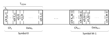
Figure 1: OFDM symbol structure

This section models a DFRC system where an OFDM transmit signal is used to simultaneously communicate with a user and sense a point target. Fig. 1 depicts an OFDM block containing $M$ OFDM symbols. Each OFDM symbol has $K$ subcarriers, with an additional $K_{G}$ subcarriers of cyclic prefix (CP). We assume that a targer’s range and velocity remain unchanged over such a block.

Let $B$ denote the signal bandwidth, corresponding to a delay resolution of $\Delta\tau=1/B$. We assume that the target round-trip delay is shorter than the CP duration (the maximal delay that can be estimated is $\tau_{\max}={K_{G}/B}$). Let $T_{\text{OFDM}}=(K+K_{G})/B\overset{\bigtriangleup}{=}K_{T}/B$ denote the OFDM symbol duration. Hence, the radar coherent processing interval equals $MT_{\text{OFDM}}$, corresponding to a Doppler resolution of $\Delta f_{D}=1/(MT_{\text{OFDM}})=B/(K_{T}M)$.

Consider the presence of a target at a distance $R$ and moving at velocity $v$ w.r.t the radar. For a monostatic configuration, $R$ and $v$ are captured on the echo signal by its time delay $\tau=2R/c$ and Doppler frequency $f_{D}=f_{c}(2v/c)$, which can be represented as follows:

$$\tau =(n_{0}+n_{\epsilon})\Delta\tau,\hskip 8.53581ptn_{0}\in\{0,~{}1,~{}\cdots,~{}K_{G}-1\},$$ (1)

$$f_{D} =(v_{0}+v_{\epsilon})\Delta f_{D},\hskip 8.53581ptv_{0}\in\left\{-\frac{M}{2},~{}\cdots,~{}0,~{}\cdots,~{}\frac{M-1}{2}\right\},$$ (2)

for $n_{\epsilon}\in(0,1)$ and $~{}v_{\epsilon}\in\left(-\frac{1}{2},~{}\frac{1}{2}\right)$. In (1) and (2), $(n_{0},~{}v_{0})$ denotes the target’s delay-Doppler bin, the parameter of interest in this paper.

Let $X[k,~{}m]$ denote the CS at the $k^{\text{th}}~{}(k=0,~{}\cdots,~{}K-1)$ subcarrier of the $m^{\text{th}}~{}(m=0,~{}\cdots,~{}M-1)$. After a $K$-point IDFT, let $x[n,~{}m]~{}(n=0,~{}\cdots,~{}K-1)$ denote the resulting time domain signal. After adding the CP, we obtain the following signal:

$$x_{\text{CP}}[n,~{}m]=\begin{cases}x[K-K_{G}+n,~{}m],&n\in\{0,~{}\cdots,~{}K_{G}-1\},\\ x[n-K_{G},~{}m],&n\in\{K_{G},~{}\cdots,~{}K_{T}-1\}.\end{cases}$$ (3)

The radar return at the transceiver (after sampling at $t=(n+mK_{T})/B$) is given by:

$$y_{\text{CP}}[n,~{}m]$$

$$= ax_{\text{CP}}[n-n_{0},~{}m]\exp\left\{{j2\pi\frac{f_{D}}{B}(n+mK_{T})}\right\}+w[n,~{}m]$$

$$= a~{}\exp\left\{{j2\pi f_{D}n/B}\right\}x_{\text{CP}}[n-n_{0},~{}m]\exp\left\{{j2\pi\frac{v_{0}+v_{\epsilon}}{M}m}\right\}+w[n,~{}m]$$ (4)

$$\approx ax_{\text{CP}}[n-n_{0},~{}m]\exp\left\{{j2\pi\frac{v_{0}+v_{\epsilon}}{M}m}\right\}+w[n,~{}m],$$ (5)

where (i) $a\in{\mathbb{C}}$ is the scattering coefficient of the target, assumed to be unchanged throughout the OFDM block, (ii) $\exp\left\{{j2\pi f_{D}n/B}\right\}\approx 1$, since typically $f_{D}\ll B$, and (iii) $w[n,~{}m]\sim\mathcal{CN}(0,~{}\sigma_{N}^{2})$ is the additive noise. After removing the CP, we get:

$$y[n,~{}m] \approx ax[n-n_{0},~{}m]\exp\left\{{\frac{j2\pi(v_{0}+v_{\epsilon})m}{M}}\right\}+w[n,~{}m],$$ (6)

where $x[n-n_{0},~{}m]$ represents a circular shift of $n_{0}$ following (3). After a $K$-point DFT, we get the frequency-domain signal:

$$Y[k,~{}m] =\mu_{k,m}(\boldsymbol{\theta_{0}})+W[k,~{}m],$$ (7a)

$$\mbox{where}~{}\mu_{k,m}(\boldsymbol{\theta_{0}}) \overset{\vartriangle}{=}aX[k,~{}m]\exp\left\{{-j2\pi\frac{n_{0}k}{K}}\right\}\exp\left\{{j2\pi\frac{(v_{0}+v_{\epsilon})m}{M}}\right\},$$ (7b)

$$\mbox{and}~{}W[k,~{}m] \sim\mathcal{CN}(0,~{}\sigma_{N}^{2}).$$ (7c)

In (7a)-(7c), $\boldsymbol{\theta_{0}}:=[n_{0},~{}v_{0},~{}v_{\epsilon},~{}A_{0},~{}\phi_{0}]^{T}$ involves all of the unknown parameters in the system, with $A_{0}$ and $\phi_{0}$ denoting the amplitude and phase of $a$.

III Characterizing the ML estimator’s OP

This section begins by formulating the ML estimator for $(n_{0},v_{0})$ over an OFDM block. We then derive the OP of this estimator. The OP is then approximated by its upper bound to yield a tractable metric that can be optimized w.r.t the input distribution.

III-A ML estimator

From (7a)-(7c), the joint probability density function of $Y[k,~{}m]$, conditioned on $\boldsymbol{\theta_{0}}$, is given by:

$$f(\mathbf{y}|\boldsymbol{\theta}_{0}) =\frac{1}{{(\pi\sigma^{2})}^{KM}}~{}\exp\left\{-\frac{1}{\sigma^{2}}\sum_{m=0}^{M-1}\sum_{k=0}^{K-1}\Big{|}Y[k,~{}m]-\mu_{k,m}(\boldsymbol{\theta}_{0})\Big{|}^{2}\right\},$$ (8)

where $\mathbf{y}:=[\mathbf{y}^{T}_{0},~{}\cdots,~{}\mathbf{y}^{T}_{M-1}]^{T}$ with $\mathbf{y}_{m}:=[Y[0,~{}m],~{}\cdots,~{}Y[K-1,~{}m]]^{T}$. The ML estimate of $\boldsymbol{\theta}_{0}$, denoted by $\hat{\boldsymbol{\theta}}$, is given by:

$$\hat{\boldsymbol{\theta}}= \arg\max_{\boldsymbol{\theta}_{0}}~{}\log f({\mathbf{y}}|\boldsymbol{\theta}_{0})$$ (9a)

$$= 2A_{0}\mathfrak{R}\left\{e^{-j\phi_{0}}\sum_{m,k}Y[k,~{}m]X[k,~{}m]^{*}e^{j2\pi\frac{n_{0}k}{K}}e^{-j2\pi\frac{(v_{0}+v_{\epsilon})m}{M}}\right\}$$

$$-\sum_{m,k}\left[|Y[k,~{}m]|^{2}+|A_{0}X[k,~{}m]|^{2}\right],$$ (9b)

Remark 1.

$v_{\epsilon}$ cannot be estimated accurately from ${\mathbf{y}}$ due to the Doppler resolution limit. However, its randomness manifests as a nuisance parameter in (9b) that affects the estimation of the other parameters in $\boldsymbol{\theta}_{0}$. Hence, we first derive the ML estimator of $(n_{0},~{}v_{0},~{}A_{0},~{}\phi_{0})$ by neglecting $v_{\epsilon}$ in (9b). Later on, we consider the impact of $v_{\epsilon}$ on the OP of this estimator by assuming $v_{\epsilon}$ to be uniformly distributed between $[-1/2,~{}1/2]$.

From the above remark, the ML estimator of $(n_{0},~{}v_{0})$ is given by:

$$(\hat{n},~{}\hat{v})= \arg\underset{(n,~{}v)}{\max}~{}\Bigg{|}\sum_{m,~{}k}Y[k,~{}m]X[k,~{}m]^{*}e^{j2\pi\frac{nk}{K}}e^{-j2\pi\frac{vm}{M}}\Bigg{|}$$ (10a)

$$= \arg\underset{(n,~{}v)}{\max}~{}\Bigg{|}\sum_{m,~{}k}Ap_{k,m}e^{j2\pi\frac{nk}{K}}e^{-j2\pi\frac{vm}{M}}e^{j2\pi\frac{v_{\epsilon}m}{M}}+w_{i}[n,~{}v]\Bigg{|}$$ (10b)

$$\overset{\Delta}{=} \arg\underset{(n,~{}v)}{\max}\>\>|\gamma_{n,v,\epsilon}|,$$ (10c)

where

$$p_{k,m} :=|X[k,~{}m]|^{2},$$ (10d)

$$\gamma_{n,v,\epsilon} :=r_{n,v,\epsilon}+w_{o}[n,~{}v],$$ (10e)

$$r_{n,v,\epsilon} :=\sum_{m,k}p_{k,m}e^{j2\pi\frac{nk}{K}}e^{-j2\pi\frac{vm}{M}}e^{j2\pi\frac{v_{\epsilon}m}{M}},$$ (10f)

$$w_{o}[n,~{}v]= \frac{1}{A_{0}}\sum_{m,~{}k}w[k,~{}m]X[k,~{}m]^{*}e^{j2\pi\frac{nk}{K}}e^{-j2\pi\frac{vm}{M}},$$ (10g)

for $n\in\{0,~{}\cdots,~{}K_{G}-1\},~{}v\in\{-M/2,~{}\cdots,~{}M/2-1\}$.

Remark 2.

$p_{k,m}$ in (10d) denotes the CS power at the $k$-th subcarrier and $m$-th OFDM symbol, $r_{n,v,\epsilon}$ in (10f) represents the discrete AF of the transmitted signal, and $\gamma_{n,v,\epsilon}$ the cross correlation between the transmitted signal and the received distorted signal. For $(n_{0},v_{0})=(0,0)$, Fig. 2 plots $|r_{n,v,\epsilon}|$ and $|\gamma_{n,v,\epsilon}|$ for: (a) BPSK input (i.e., constant magnitude CSs) and $v_{\epsilon}=0$, (b) 64-QAM input (i.e., varying magnitude CSs) and $v_{\epsilon}=0$), and (c) BPSK input with $v_{\epsilon}\neq 0$. To successfully locate $(n_{0},~{}v_{0})$ from $\gamma_{n,v,\epsilon}$, it is desirable for the peak lobe at $r_{0,0,\epsilon}$ to be easily distinguishable from its side lobes. Eqn. (10f) and Figs. 2b and 2c show that CSs with varying magnitudes, as well as $v_{\epsilon}\neq 0$, lead to AF sidelobes, which would increase the OP. While the sidelobes due to $v_{\epsilon}$ are unavoidable (see Remark 1), the sidelobes due to CS magnitudes can be suppressed through careful design of the input distribution. This motivates the problem of minimizing the OP w.r.t the input distribution, considering the effect of the continuous velocity for better radar performance.

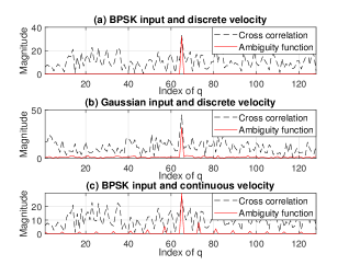
Figure 2: The magnitudes of discrete AF and the corresponding cross correlation with uniform power allocation given BPSK/Gaussian input and discrete/continuous velocity, with $K=32$, $M=16$ and $K_{G}=8$. The index, $q$, is related to range-Doppler bin $(n,~{}v)$ as follows: $q=n+(v+M/2)K_{G}$.

III-B ML-based radar metric

A metric that directly characterizes the ML estimator’s sensing performance is the OP – the probability of incorrectly estimating $(n_{0},v_{0})$. Without loss of generality, we assume $(n_{0},v_{0})=(0,0)$ for ease of analysis.

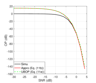
Figure 3: The simulated and approximated OP for $K=32$, $K_{G}=8$, $M=8$.

To account for the randomness of $v_{\epsilon}$, we assume it is uniformly distributed over $[-1/2,~{}1/2]$, and consider the OP averaged over $v_{\epsilon}$. This quantity, denoted by ${\mathbb{P}}_{\text{o}}$, is the probability that the sidelobe magnitudes ($|\gamma_{n,v}|$ for $(n,~{}v)\neq(0,~{}0)$) is larger than the main lobe magnitude ($|\gamma_{0,0}|$), which can be expressed as follows:

$${\mathbb{P}}_{\rm o} :=\mathbb{E}_{v_{\epsilon}}\left\{{\mathbb{P}}\left[\bigcup_{n,v,\epsilon}\left\{|\gamma_{n,v,\epsilon}|>|\gamma_{0,0,\epsilon}|\right\}\right]\right\}$$ (11a)

$$\leq\mathbb{E}_{v_{\epsilon}}\left\{\sum_{(n,~{}v)\neq(0,~{}0)}{\mathbb{P}}\left[|\gamma_{n,v,\epsilon}|>|\gamma_{0,0,\epsilon}|\right]\right\}$$ (11b)

$$\approx\mathbb{E}_{v_{\epsilon}}\left\{\sum_{(n,~{}v)\neq(0,~{}0)}\exp\left\{-\frac{|r_{0,0,\epsilon}|}{2\sigma^{2}}\right\}I_{0}\left(\frac{|r_{n,v,\epsilon}|}{2\sigma^{2}}\right)/2\right\}$$ (11c)

$$\leq\mathbb{E}_{v_{\epsilon}}\left\{\sum_{(n,~{}v)\neq(0,~{}0)}\exp\left\{-\frac{|r_{0,0,\epsilon}|-|r_{n,v,\epsilon}|}{2\sigma^{2}}\right\}/2\right\}$$ (11d)

$$\overset{\triangle}{=}{\mathbb{P}}_{\rm UB},$$ (11e)

where $\sigma^{2}=\sigma_{N}^{2}/A^{2}$. The inequality in (11b) stems from the union bound, while the upper bound in (11d), termed the UBOP, is more tractable for optimization w.r.t the input distribution than ${\mathbb{P}}_{o}$. Hence, we adopt the UBOP as the radar metric from hereon. The derivation for (11d) is provided in Appendix LABEL:sec_App_OP and is shown to be tight in the SNR region of interest (i.e., the threshold region) in Fig. 3.

Remark 3.

The expression in (11d) captures the relationship between the AF and the UBOP. Specifically, with a low SNR in (11d), $\sum_{(n,~{}v)\neq(0,~{}0)}\exp\left\{-{|r_{0,0,\epsilon}|}/{2\sigma^{2}}\right\}\approx\sum_{(n,~{}v)\neq(0,~{}0)}-{|r_{0,0,\epsilon}|}/{2\sigma^{2}}$, which indicates that the UBOP can be approximated by the integrated-side-to-peak-lobe-difference (ISPLD) of the AF in this regime. On the contrary, given a high SNR, the maximal exponential term in (11d) dominates. Hence, the UBOP in this regime can be approximated by the peak-to-the-largest-side-lobe difference.

Remark 4.

From (10f) and (11d), the UBOP is a function of the CS input distribution through $p_{k,m}$. This motivates the problem of minimizing the UBOP w.r.t the input distribution, which we consider in the following section.

IV Minimizing OP for Constant Magnitude Input

In this section, we minimize the UBOP for constant magnitude CSs (with PSK input). In this scheme, the UBOP ${\mathbb{P}}_{\rm UB}$ is deterministic regardless of the random information carried by CSs’ phases. Hence, this scheme is able to achieve the same radar performance in DFRC as that of using deterministic OFDM signals in pure radar system. Hence, studying scheme helps to provide a performance benchmark for the scheme with random CS magnitudes in the future, and provide insight into radar-beneficial signals.

IV-A Problem formulation

For the special case of constant CS magnitude, the UBOP is a deterministic function of $p_{k,m}$ – i.e., the power allocation across subcarriers and OFDM symbols – and is independent of the input distribution. Hence, we formulate the following optimization problem: {p_k,m} P_UB in (11d), ∑_k, m p_k,m ≤P^max, where $P^{\max}$ is the transmit power constraint. For the above problem, we have the following result:

Lemma 1.

In a point target scenario, for any $(n_{0},~{}v_{0})$, the optimal power allocation across subcarriers ($p_{k,m}$ across $k$ for $\forall~{}m$) to minimize ${\mathbb{P}}_{\rm UB}$ is the uniform power allocation.

Proof:

Let $p_{m}:=\sum_{k}~{}p_{k,m}$ denote the total power of the $m^{\text{th}}$ OFDM symbol. The expectation over $v_{\epsilon}$ in (11d) is approximated by taking multiple samples of $v_{\epsilon}$ from the set $\{\epsilon_{1},~{}\cdots,~{}\epsilon_{|\kappa|}\}$ (denoted by set $\kappa$, the larger the number of samples, the more accurate the approximation) following its uniform distribution. Hence, ${\mathbb{P}}_{\rm UB}$ becomes:

$${\mathbb{P}}_{\rm UB}$$

$$\approx \frac{1}{|\kappa|}\sum_{{\epsilon}\in\kappa}\sum_{(n,~{}v)\neq(0,~{}0)}\exp\left\{-\frac{|r_{0,0,\epsilon}|-|r_{n,v,\epsilon}|}{2\sigma^{2}}\right\}\hskip 8.53581pt(\mbox{for large }|\kappa|)$$ (12a)

$$= \frac{\sum_{{\epsilon}\in\kappa}}{|\kappa|}\left(\sum_{n=0,~{}v\neq 0}\exp\left\{-\frac{|r_{0,0,\epsilon}|-|r_{n,v,\epsilon}|}{2\sigma^{2}}\right\}\right.$$ (12b)

$$\left.~{}~{}~{}~{}~{}~{}~{}~{}~{}~{}~{}~{}~{}~{}+\sum_{~{}n\neq 0}\exp\left\{-\frac{|r_{0,0,\epsilon}|-|r_{n,v,\epsilon}|}{2\sigma^{2}}\right\}\right)$$ (12c)

$$\geq \frac{\sum_{{\epsilon}\in\kappa}}{|\kappa|}\left(\sum_{v\neq 0}\exp\left\{-\frac{|r_{0,0,\epsilon}|-|r_{0,v,\epsilon}|}{2\sigma^{2}}\right\}+\sum_{n\neq 0}\exp\left\{-\frac{|r_{0,0,\epsilon}|}{2\sigma^{2}}\right\}\right)$$ (12d)

$$= \frac{\mathbf{1}^{T}}{|\kappa|}\exp\left\{-\frac{{\mathbf{1}^{M-1}}\otimes|\mathbf{r}_{0}|-|\mathbf{r^{\prime}}|}{2\sigma^{2}}\right\}+\frac{(K_{G}-1)M}{|\kappa|}\mathbf{1}^{T}\exp\left\{-\frac{|\mathbf{r}_{0}|}{2\sigma^{2}}\right\}$$ (12e)

$$\overset{\triangle}{=} {\mathbb{P}}_{\rm UB}(\mathbf{r}),$$ (12f)

where

$$\mathbf{r}_{m}= \left[r_{0,m,\epsilon_{1}},~{}\cdots,~{}r_{0,m,\epsilon_{|\kappa|}}\right]^{T},$$ (12g)

$$\mathbf{r^{\prime}}:= [\mathbf{r}_{1}^{T},~{}\cdots,~{}\mathbf{r}_{M-1}^{T}]^{T},$$ (12h)

$$\mathbf{r}:= [\mathbf{r}_{0}^{T},~{}\mathbf{r^{\prime}}^{T}]^{T}=[\mathbf{r}_{0}^{T},~{}\cdots,~{}\mathbf{r}_{M-1}^{T}]^{T}=\mathbf{F}^{D}\mathbf{p}_{M},$$ (12i)

$$\mathbf{p}_{M}:= [p_{0},~{}\cdots,~{}p_{M-1}]^{T},$$ (12j)

$$\mathbf{F}^{D}:= [\mathbf{f}^{D,0,\epsilon_{1}},~{}\mathbf{f}^{D,0,\epsilon_{|\kappa|}},~{}\cdots,~{}\mathbf{f}^{D,~{}M-1,\epsilon_{1}},~{}\mathbf{f}^{D,~{}M-1,\epsilon_{|\kappa|}}]^{T},$$ (12k)

$$\mathbf{f}_{m}^{D,v,\epsilon_{l}}= e^{-j2\pi{m(v-{\epsilon_{l}})}/{M}},$$ (12l)

where (12d) is achieved because $|r_{n,v,\epsilon}|\geq 0$ for $n\neq 0$ with the equality achieved if and only if $p_{k,m}=p_{m}/K$ since $r_{n,v,\epsilon}=\sum_{m,k}p_{m}/Ke^{j2\pi\frac{nk}{K}}e^{-j2\pi\frac{vm}{M}}e^{j2\pi\frac{v_{\epsilon}m}{M}}=\sum_{k}e^{j2\pi\frac{nk}{K}}\sum_{m}p_{m}e^{-j2\pi\frac{vm}{M}}e^{j2\pi\frac{v_{\epsilon}m}{M}}/K=0$. Since in (12d), the only variables involved are the power allocation across symbols, i.e., $p_{m}$ ($r_{0,v,\epsilon}=\sum_{m}p_{m}e^{-j2\pi\frac{vm}{M}}e^{j2\pi\frac{v_{\epsilon}m}{M}}$), we show that the optimal power allocation would have uniform power allocation across sub-carriers, after which we need to optimize the power allocation across OFDM symbols $p_{m}$.

∎

After adopting the optimal power allocation across subcarriers, the optimization problem (IV-A) becomes: p_M, rP_UB(r) in (12e), 1^T p_M ≤P^max r=F^Dp_M.

IV-B Low complexity optimization

Solving problem (1) can be very time-consuming with a large number of OFDM symbols $M$, whereas in OFDM radar, $M$ shall be large, i.e., above $512$, to achieve a high resolution of velocity [sturm2011waveform]. Hence, in this section, we propose a low-complexity ADMM algorithm where problem (1) is approximately solved in an iterative manner with closed-form solutions in each round.

Considering the linear constraint in (1), we adopt the ADMM algorithm to iteratively update $\mathbf{p}_{M}$ and $\mathbf{r}_{v}$ until the two successive solutions get close [bertsekas2014constrained]. Following the ADMM structure, at the $l^{\text{th}}$ iteration, problem (1) is iteratively formulated as:

$$\mathbf{r}^{(l+1)} :=\arg\min\left\{{\mathbb{P}}_{\rm UB}(\mathbf{r})+\frac{\rho}{2}\|\mathbf{r}-\mathbf{F}^{D}\mathbf{p}_{M}^{(l)}+\mathbf{d}^{(l)}\|^{2}\right\},$$ (13)

$$\mathbf{p}_{M}^{(l+1)} :=\arg\min\left\{\mathbbm{1}(\mathbf{1}^{T}\mathbf{p}_{M}\leq P^{\max})+\frac{\rho}{2}\|\mathbf{r}^{(l+1)}-\mathbf{F}^{D}\mathbf{p}_{M}+\mathbf{d}^{(l)}\|^{2}\right\},$$ (14)

$$\mathbf{d}^{(l+1)} :=\mathbf{d}^{(l)}+\mathbf{r}^{(l+1)}-\mathbf{F}^{D}\mathbf{p}_{M}^{(l+1)},$$ (15)

where $\mathbf{d}^{(l)}$ is the ADMM stepsize at the $l^{\text{th}}$ iteration and $\rho$ is the ADMM penalty coefficient.

IV-B1 Updating $\mathbf{r}$

To solve problem (13), we adopt the SCP to approximate the exponential function in (13) linearly by the first-order Taylor expansion. The optimal solution of this approximated problem is then used as a new operating point of the Taylor expansion for the next SCP round. The procedure is repeated until two successive solutions are close enough.

Consequently, assume that $\mathbf{r}^{(l+1,t)}$ is the optimal solution at the $t^{\text{th}}$ iteration of SCP. Then $\mathbf{r}^{(l+1,~{}t+1)}$ is updated as:

$$\mathbf{r}^{(l+1,~{}t+1)} =\arg\min\left\{{\boldsymbol{\alpha}^{(l+1,~{}t)}}^{T}|\mathbf{r}|+\frac{\rho}{2}\|\mathbf{r}-\mathbf{F}^{D}\mathbf{p}_{M}^{(l)}\|^{2}\right\}$$ (16a)

$$=\left(\mathbf{F}^{D}\mathbf{p}_{M}^{(l)}-\frac{\boldsymbol{\theta}^{(l)}\odot\boldsymbol{\alpha}^{(l+1,~{}t)}}{\rho}\right)^{+},$$ (16b)

where $\boldsymbol{\theta}^{(l)}=\angle\mathbf{F}^{D}\mathbf{p}_{M}^{(l)}$. The closed-form expression in (16b) is derived in Appendix LABEL:sec_APP_OPT. The first-order Taylor coefficient $\boldsymbol{\alpha}^{(l+1,~{}t)}=[{\boldsymbol{\alpha}_{0}^{(l+1,~{}t)}}^{T},~{}\cdots,~{}{\boldsymbol{\alpha}_{M-1}^{(l+1,~{}t)}}^{T}]^{T}$ is expressed in (17).

$$\boldsymbol{\alpha}_{v}^{(l+1,t)}=\begin{cases}-\sum_{v=1}^{M-1}\exp\left\{-\frac{|{\mathbf{r}_{0}^{(l+1,t)}}|-|{\mathbf{r}_{v}^{(l+1,t)}}|}{2\sigma^{2}}\right\}/{\left(2\sigma^{2}{|\kappa|}\right)}-(K_{G}-1)M\exp\left\{-\frac{|{\mathbf{r}_{0}^{(l+1,t)}}|}{2\sigma^{2}}\right\}/{\left(2\sigma^{2}{|\kappa|}\right)},&\text{ for }v=0;\\ \exp\left\{-\frac{|{\mathbf{r}_{0}^{(l+1,t)}}|-|{\mathbf{r}_{v}^{(l+1,t)}}|}{2\sigma^{2}}\right\}/{\left(2\sigma^{2}{|\kappa|}\right)},&\text{ otherwise.}\end{cases}$$ (17)

 

IV-B2 Updating $\mathbf{p}_{M}$

Given a fixed $\mathbf{r}^{(l+1)}$, the optimal $\mathbf{p}_{M}^{(l+1)}$ can be directly solved by quadratic programming (QP) as: p_Mρ2∥r^(l+1)-F^Dp_M∥^2, 1^T p_M ≤P^max. The algorithm is summarized in Algorithm 1.

Input: $l\leftarrow 0,~{}\mathbf{r}^{(0)},~{}\mathbf{p}_{M}^{(0)},~{}\rho,~{}\epsilon_{S}>0$

Output: ${\mathbf{p}}_{M}$;

Repeat:

1. Update $\mathbf{r}^{(l+1)}$ in problem (13) by SCP in Algorithm 2

2. Update $\mathbf{p}_{M}^{(l+1)}$ in problem (14)

3. $l\leftarrow l+1$; ${\mathbf{p}}_{M}\leftarrow\mathbf{p}_{M}^{(l+1)}$

4. Quit if $\|\mathbf{p}_{M}^{(l+1)}-\mathbf{p}_{M}^{(l)}\|/\|\mathbf{p}_{M}^{(l+1)}\|<\epsilon_{S}$

Algorithm 1 ADMM for PSK input

Input: $t\leftarrow 0,~{}\mathbf{r}^{(l+1,0)},~{}\epsilon_{0}$

Output: $\mathbf{r}^{(l+1)}$

Repeat:

1. Compute $\boldsymbol{\alpha}^{(l+1,~{}t)}$ in (17) at the operating point $\mathbf{r}^{(l+1,~{}t)}$

2. Compute $\mathbf{r}^{(l+1,~{}t+1)}$ using (16b)

3. $t\leftarrow t+1$; $\mathbf{r}^{(l+1)}\leftarrow\mathbf{r}^{(l+1,~{}t+1)}$

4. Quit if $\|\mathbf{r}^{(l+1,~{}t+1)}-\mathbf{r}^{(l+1,~{}t)}\|<\epsilon_{0}\|\mathbf{r}^{(l+1,~{}t+1)}\|$

Algorithm 2 SCP

V Minimizing OP for Random Magnitude Input (Gaussian)

This section evaluates the radar performance in OFDM DFRC with asymmetric Gaussian input, where the magnitude of the CSs becomes a random variable obeying the Rician distribution. Consequently, we evaluate the aUBOP and then optimize the Gaussian mean and variance at each symbol’s subcarriers to minimize the aUBOP. In this scheme, an achievable communication constraint is added to avoid a zero-variance optimization result where no information bits are transmitted.

V-A Problem formulation

In this context, we first model the CS $X[k,~{}m]$ in (3) as a complex non-zero mean asymmetric Gaussian variable:

$$X[k,~{}m]=X_{R}[k,~{}m]+jX_{I}[k,~{}m],$$ (18)

where $X_{R/I}[k,~{}m]\sim\mathcal{N}(\mu^{R/I}_{k,m},~{}{\sigma^{R/I}_{k,m}}^{2})$.

Denote by $\overline{p}^{R/I}_{k,m}$ the average power (second-order moments) allocated to the real and imaginary part of the $m^{\text{th}}$ OFDM symbol at the $k^{\text{th}}$ subcarrier, we have:

$$\overline{p}^{R/I}_{k,m} ={\mu^{R/I}_{k,m}}^{2}+{\sigma^{R/I}_{k,m}}^{2}.$$ (19)

On this basis, the ambiguity function $r_{n,v,\epsilon}$ in (11d) becomes random, making the UBOP varying. Hence, we derive the aUBOP as follows:

$$\overline{{\mathbb{P}}}_{\rm UB}\left(\overline{\mathbf{p}},~{}\boldsymbol{\sigma}\right)= \mathbb{E}_{v_{\epsilon},~{}X[k,~{}m]}\left\{\sum_{(n,~{}v)\neq(0,~{}0)}\exp\left\{-\frac{|r_{0,0,\epsilon}|-|r_{n,v,\epsilon}|}{2\sigma^{2}}\right\}/2\right\}$$ (20a)

$$\overset{\nearrow}{\approx} \frac{1}{4\sigma^{2}}\sum_{(n,~{}v)\neq(0,~{}0)}\mathbb{E}_{v_{\epsilon},~{}X[k,~{}m]}\left\{-{|r_{0,0,\epsilon}|+|r_{n,v,\epsilon}|}\right\}$$ (20b)

$$\ \leq \frac{1}{4\sigma^{2}}\sum_{(n,~{}v)\neq(0,~{}0)}\mathbb{E}_{v_{\epsilon}}\left\{-|\mathbb{E}_{X[k,~{}m]}\left\{r_{0,0,\epsilon}\right\}|\right.$$ (20c)

$$\left.+\sqrt{\mathbb{E}_{X[k,~{}m]}\left\{|r_{n,v,\epsilon}|^{2}\right\}}\right\}$$ (20d)

$$= \frac{1}{4|\kappa|\sigma^{2}}\sum_{\epsilon\in\kappa}\sum_{(n,~{}v)\neq(0,~{}0)}-\sqrt{\overline{\mathbf{p}}^{T}\mathbf{A}^{\epsilon}\overline{\mathbf{p}}}+g^{(n,v,\epsilon)}\left(\overline{\mathbf{p}},\boldsymbol{\sigma}\right),$$ (20e)

$$\mbox{with}~{}\mathbf{\overline{p}}:= \left[\mathbf{\overline{p}}^{T}_{R,~{}0},..,\mathbf{\overline{p}}^{T}_{R,~{}m-1},~{}\cdots,~{}\mathbf{\overline{p}}^{T}_{I,~{}0},~{}\cdots,~{}\mathbf{\overline{p}}^{T}_{I,~{}m-1}\right]^{T},$$ (20f)

$$\mathbf{\overline{p}}_{R/I,~{}m}:= [\overline{p}^{R/I}_{0,m},~{}\cdots,~{}\overline{p}^{R/I}_{K-1,m}]^{T},$$ (20g)

$$\boldsymbol{\sigma}:= \left[\boldsymbol{\sigma}^{T}_{R,~{}0},..,\boldsymbol{\sigma}^{T}_{R,~{}m-1},~{}\cdots,~{}\boldsymbol{\sigma}^{T}_{I,~{}0},~{}\cdots,~{}\boldsymbol{\sigma}^{T}_{I,~{}m-1}\right]^{T},$$ (20h)

$$\boldsymbol{\sigma}_{R/I,~{}m}:= \left[{\sigma^{R/I}_{0,m}}^{2},~{}\cdots,~{}{\sigma^{R/I}_{K-1,m}}^{2}\right]^{T},$$ (20i)

$$g^{(n,~{}v,~{}\epsilon)}\left(\overline{\mathbf{p}},~{}\boldsymbol{\sigma}\right)= \sqrt{\mathbf{\overline{p}}^{T}\mathbf{A}^{(n,~{}v,~{}\epsilon)}\mathbf{\overline{p}}-2\|\overline{\mathbf{p}}-\boldsymbol{\sigma}\|^{2}},$$ (20j)

$$\mathbf{A}^{\epsilon}= \mathfrak{R}\left\{{\mathbf{f}_{D_{0}}^{\epsilon}}\right\}\mathfrak{R}\left\{{\mathbf{f}_{D_{0}}^{\epsilon}}\right\}^{T}+\mathfrak{I}\left\{{\mathbf{f}_{D_{0}}^{\epsilon}}\right\}\mathfrak{I}\left\{{\mathbf{f}_{D_{0}}^{\epsilon}}\right\}^{T},$$ (20k)

$$\mathbf{A}^{(n,~{}v,~{}\epsilon)}= {\mathbf{f}_{R}^{(n,~{}v,~{}\epsilon)}}{\mathbf{f}_{R}^{(n,~{}v,~{}\epsilon)}}^{T}+{\mathbf{f}_{I}^{(n,~{}v,~{}\epsilon)}}{\mathbf{f}_{I}^{(n,~{}v,~{}\epsilon)}}^{T}+2\mathbf{I}^{2KM},$$ (20l)

where (20b) assumes low SNR at the radar’s receiver, giving $\exp\{x\}\rightarrow x+1$ for $x\rightarrow 0$ ($r_{0,0}\geq r_{n,v}$ for any $(n,~{}v)$) (neglecting the constant term, the $\overset{\nearrow}{\approx}$ in (20b) means approximately increasing with). (20d) is due to the concavity of the square root function. (20e) is achieved from Appendix LABEL:sec_App_2nd_monents. In (20k), $\mathbf{f}_{D_{0}}^{\epsilon}=\mathbf{1}^{2}\otimes\left(\mathbf{f}^{D,~{}0,~{}\epsilon}\otimes\mathbf{1}^{K}\right)\in\mathbb{R}^{2KM}$. In (20l), $\mathbf{f}_{R/I}^{(n,~{}v,~{}{\epsilon})}=\mathfrak{R/I}\left\{\mathbf{1}^{2}\otimes\left(\mathbf{f}^{D,~{}v,~{}{\epsilon}}\otimes\mathbf{f}^{R,~{}n}\right)\right\}\in\mathbb{C}^{2KM}$ with $\mathbf{f}^{R,~{}n}\in\mathbb{C}^{K}$ for $\mathbf{f}^{R,~{}n}_{k}=e^{j2\pi{nk}/{K}}$ and $\mathbf{f}^{D,~{}v,~{}{\epsilon}}\in\mathbb{C}^{M}$ for $\mathbf{f}^{D,~{}v,~{}{\epsilon}}_{m}=e^{-j2\pi{m(v-{\epsilon})}/{M}}$.

Remark 5.

(20e) indicates that the optimization objective, aUBOP$\left(\overline{\mathbf{p}},~{}\boldsymbol{\sigma}\right)$, finally becomes a scaling term of the average ISPLD in low SNR, corresponding to Remark 2. Also, (20e) indicates that, without communication constraints, the optimal solution to minimize (20e) must have $|\mu_{k,m}|^{2}=\overline{p}_{k,m}$, which means that all the power is allocated to the deterministic component. In other words, the randomness of the CS magnitudes degrades radar’s OP.

V-B Optimization

We then formulate the corresponding optimization problem in DFRC using the developed metric in (20e). With the constraint on achievable rate, we have the optimization problem (neglecting the constant multiplier $1/(4\sigma^{2})$): ¯p, σ∑_ϵ∈κ∑_(n, v)≠(0, 0)-¯p^TA^ϵ¯p+g^(n, v, ϵ)(¯p, σ), 1^T¯p≤P^max c_0^T log(1+c_1⊙σ )≥R^c ¯p ≥σ σ≥0, where $\mathbf{c}_{0}=\mathbf{1}^{2KM}/({2KM})$ and $\mathbf{c}_{1}={\mathbf{1}^{2M}\otimes\mathbf{c}}\in\mathbb{R}^{2KM}$ with $\mathbf{c}_{k}={2K|h_{k}|^{2}}/({B\sigma^{2}})$ for $k=[1,~{}\cdots,~{}K]$. $h_{k}$ is the communication channel for the $k^{\text{th}}$ subcarrier. $R^{c}$ refers to the minimum sum rate for communications.

For efficiency, we use BCD to solve problem (V-B). In BCD, given an initial point of $\overline{\mathbf{p}}^{(l)}/\boldsymbol{\sigma}^{(l)}$ at the $l^{\text{th}}$ iteration, $\overline{\mathbf{p}}^{(l+1)}$ is optimized first with fixed $\boldsymbol{\sigma}^{(l)}$. Then $\boldsymbol{\sigma}^{(l+1)}$ is optimized with fixed $\overline{\mathbf{p}}^{(l+1)}$. The iteration continues until two successive solutions get close.

V-B1 Updating $\mathbf{\overline{p}}$

Given $\boldsymbol{\sigma}^{(l)}$, the sub-problem for $\overline{\mathbf{p}}$ is: ¯p∑_ϵ∈κ∑_(n, v)≠(0, 0)-¯p^TA^ϵ¯p+g^(n, v, ϵ)(¯p, σ^(l)), 1^T¯p≤P^max ¯p ≥σ^(l), whose objective function in (V-B1) is non-convex. As a solution, we adopt SCP similarly to Section IV-B, where the square root function in (V-B1) is approximated by its first-order Taylor expansion: $\sqrt{x}\approx(x-x_{0})/(2\sqrt{x_{0}})+\sqrt{x_{0}}=x/(2\sqrt{x_{0}})+\sqrt{x_{0}}/2$.

Assume $\overline{\mathbf{p}}^{(t)}$ is the operating point at the beginning of the $t^{\text{th}}$ iteration when solving problem (V-B1). Then, (V-B1) at the $t^{\text{th}}$ iteration is linearly approximated as:

$$\sum_{\epsilon\in\kappa}\sum_{(n,~{}v)\neq(0,~{}0)}-\sqrt{\overline{\mathbf{p}}^{T}\mathbf{A}^{\epsilon}\overline{\mathbf{p}}}+g^{(n,~{}v,~{}\epsilon)}\left(\overline{\mathbf{p}},~{}\boldsymbol{\sigma}^{(l)}\right)$$

$$\approx \overline{\mathbf{p}}^{T}\mathbf{B}^{(l,~{}t)}\overline{\mathbf{p}}+{\boldsymbol{\alpha}^{(l,~{}t)}}^{T}\overline{\mathbf{p}}+{\alpha_{c}}^{(l,~{}t)},$$ (21a)

with

$$\mathbf{B}^{(l,~{}t)}= \sum_{\epsilon\in\kappa}\sum_{(n,~{}v)\neq(0,~{}0)}\mathbf{A}^{(n,~{}v,~{}\epsilon)}/\left(2g^{(n,~{}v,~{}\epsilon)}\left(\overline{\mathbf{p}}^{(t)},~{}\boldsymbol{\sigma}^{(l)}\right)\right)$$ (21b)

$$= \left(\mathbf{F}_{R}\oslash\mathbf{g}^{(l,~{}t)}\right)\left(\mathbf{F}_{R}\oslash\mathbf{g}^{(l,~{}t)}\right)^{T}$$

$$+\left(\mathbf{F}_{I}\oslash\mathbf{g}^{(l,~{}t)}\right)\left(\mathbf{F}_{I}\oslash\mathbf{g}^{(l,~{}t)}\right)^{T}+2\|1\oslash\mathbf{g}^{(l,~{}t)}\|^{2}\mathbf{I}^{2KM},$$ (21c)

$$\boldsymbol{\alpha}^{(l,~{}t)}= -(K_{G}M-1)\sum_{\epsilon\in\kappa}\mathbf{A}^{\epsilon}\overline{\mathbf{p}}^{(t)}/\sqrt{{\mathbf{p}^{(t)}}^{T}\mathbf{A}^{\epsilon}{\mathbf{p}^{(t)}}}$$

$$-4\left(\overline{\mathbf{p}}^{(t)}-\boldsymbol{\sigma}^{(t)}\right)\|1\oslash\mathbf{g}^{(l,~{}t)}\|^{2},$$ (21d)

where ${\alpha_{c}}^{(l,~{}t)}$ is the Taylor constant that can be omitted. In (21), $\mathbf{F}_{R/I}=\begin{bmatrix}\mathbf{F}_{R/I}^{0,~{}-M/2},\mathbf{F}_{R/I}^{1,~{}-M/2},~{}\cdots,~{}\mathbf{F}_{R/I}^{K_{G}-1,~{}m/2-1}\end{bmatrix}\in\mathbb{R}^{2KM\times(K_{G}M-1)|\kappa|}$ with $\mathbf{F}_{R/I}^{n,~{}v}=\begin{bmatrix}\mathbf{f}_{R/I}^{(n,~{}v,~{}\epsilon_{1})},~{}\cdots,~{}\mathbf{f}_{R/I}^{(n,~{}v,~{}\epsilon_{|\kappa|})}\end{bmatrix}\in\mathbb{R}^{2KM\times|\kappa|}$ (neglecting $\mathbf{F}_{R/I}^{0,~{}0}$). Similarly, in (21), $\mathbf{g}^{(l,~{}t)}=\left[4{\mathbf{q}^{(t)}+8\|\overline{\mathbf{p}}^{(t)}\|^{2}-8\|\overline{\mathbf{p}}^{(t)}-\boldsymbol{\sigma}^{(l)}\|^{2}}\right]^{1/4}\in\mathbb{R}^{(K_{G}M-1)|\kappa|}$ with $\mathbf{q}^{(t)}={\mathbf{\overline{p}}^{(t)}}^{T}{\mathbf{F}_{R}}\odot\left({\mathbf{\overline{p}}^{(t)}}^{T}{\mathbf{F}_{R}}\right)^{*}+{\mathbf{\overline{p}}^{(t)}}^{T}\mathbf{F}_{I}\odot\left({\mathbf{\overline{p}}^{(t)}}^{T}\mathbf{F}_{I}\right)^{*}$.

Hence, we form the sub-problem towards solving problem (V-B1) as: ¯p¯p^TB^(l, t)¯p+α^(l, t)^T¯p, (V-B1)- (V-B1), which is a QP problem.

V-B2 Updating $\boldsymbol{\sigma}$

When fixing $\mathbf{\overline{p}}$ as $\mathbf{\overline{p}}^{(l)}$, we observe that the objective function in problem (V-B) is a monotonically increasing function with $2{\mathbf{\overline{p}}^{(l)}}^{T}\boldsymbol{\sigma}-\|\boldsymbol{\sigma}\|^{2}$. Hence, the sub-problem for $\boldsymbol{\sigma}$ becomes: σ2¯p^(l)^Tσ-∥σ∥^2, c_0^T log(1+c_1⊙σ )≥R^c ¯p^(l) ≥σ σ≥0, which is convex. Again, for lower complexity to handle a large number of variables, we solve problem (V-B2) iteratively by SCP with closed-form solutions. At the $t^{\text{th}}$ iteration of the SCP sub-problem, the concave objective function is approximated by the first order Taylor expansion, and the sub-problem becomes: σβ^(l, t)^Tσ, (V-B2)-  (V-B2), with $\boldsymbol{\beta}^{(l,~{}t)}=2\left(\mathbf{\overline{p}}^{(l)}-\boldsymbol{\sigma}^{(t)}\right)$. The closed-form solution for problem (V-B2), after KKT, is given by:

$$\boldsymbol{\sigma}_{q}=\begin{cases}\mathbf{\overline{p}}^{(l)}_{q},&~{}u>\boldsymbol{\beta}^{(l,~{}t)}_{q}\left(1+\mathbf{c}_{1,~{}q}{\mathbf{\overline{p}}}^{(l)}_{q}\right)/\left(\mathbf{c}_{0,~{}q}\mathbf{c}_{1,~{}q}\right);\\ 0,&~{}0<u<\boldsymbol{\beta}^{(l,~{}t)}_{q}/\left(\mathbf{c}_{0,~{}q}\mathbf{c}_{1,~{}q}\right);\\ u\mathbf{c}_{0,~{}q}/\boldsymbol{\beta}^{(l,~{}t)}_{q}-1/\mathbf{c}_{1,~{}q},&~{}\text{otherwise},\end{cases}$$ (22)

where $u$ is the Lagrangian multiplier of constraint (V-B2), obtained by bi-section search.

The entire algorithm to solve problem (V-B) is summarized in Algorithm 3.

Input: $l\leftarrow 0,~{}\overline{\mathbf{p}}^{(0)},~{}{\boldsymbol{\sigma}}^{(0)}_{R},~{}\epsilon_{S}>0$;

Output: $\overline{\mathbf{p}},~{}{\boldsymbol{\sigma}}$;

Repeat:

1. Compute $\overline{\mathbf{p}}^{(l+1)}$ in problem (V-B1) using SCP, whose solution of each sub-problem is given in problem (V-B1)

2. Compute ${\boldsymbol{\sigma}}^{(l+1)}$ in problem (V-B2) using SCP, whose closed-form solution at each iteration is given in (22)

3. $l\leftarrow l+1$; $\overline{\mathbf{p}}\leftarrow\overline{\mathbf{p}}^{(l+1)}$; ${\boldsymbol{\sigma}}\leftarrow{\boldsymbol{\sigma}}^{(l+1)}$

4. Quit if $|\overline{{\mathbb{P}}}^{(l+1)}_{\rm UB}\left(\overline{\mathbf{p}},~{}\boldsymbol{\sigma}\right)-\overline{{\mathbb{P}}}^{(l)}_{\rm UB}\left(\overline{\mathbf{p}},~{}\boldsymbol{\sigma}\right)|<\epsilon_{S}$

Algorithm 3 BCD for Gaussian input

V-C Decoupling optimization

Algorithm 3 can be time-consuming given large $K$ and $M$ because of the large-dimensional variables and coefficients. However, inspired by the optimal power allocation in section IV, we give a simplified method by decoupling the optimization of CS input distribution across time domain (OFDM symbols) and frequency domain (OFDM subcarriers), namely the decoupling method. Specifically, we assume that the distribution of CSs on each OFDM symbol is a scaled version of a common distribution $\overline{\mathbf{p}}_{K}\in\mathbb{R}^{2K}$ and $\boldsymbol{\sigma}_{K}\in\mathbb{R}^{2K}$ (accounting for the real and imaginary part). Mathematically, the final distribution of $X[k,~{}m]$ has the form:

$$\overline{\mathbf{p}}=\mathbf{F}_{M}\overline{\mathbf{p}}_{K},~{}{\boldsymbol{\sigma}}=\mathbf{F}_{M}\boldsymbol{\sigma}_{K},$$ (23)

where $\mathbf{F}_{M}=\begin{bmatrix}\mathbf{p}_{M}\otimes\mathbf{I}^{K}&\mathbf{0}^{KL\times K}\\ \mathbf{0}^{KL\times K}&\mathbf{p}_{M}\otimes\mathbf{I}^{K}\end{bmatrix}\in\mathbb{R}^{2KL\times 2K}$ with $\mathbf{p}_{M}$ being the optimal power allocation across symbols from Section IV. We define ${\mathbf{1}^{2K}}^{T}\mathbf{\overline{p}}_{K}\leq 1$ for the power constraint. Consequently, compared with optimizing $\overline{\mathbf{p}}$ and $\boldsymbol{\sigma}$ of totally $4KL$ variables in section V-B, after decoupling, we only need to optimize ${\mathbf{p}}_{M}$, $\overline{\mathbf{p}}_{K}$ and $\boldsymbol{\sigma}_{K}$ which are totally $M+4K$ variables.

On this basis, $\overline{{\mathbb{P}}}_{\rm UB}\left(\overline{\mathbf{p}},~{}\boldsymbol{\sigma}\right)$ in (20e) as a function of $\overline{\mathbf{p}}_{K}$ and $\boldsymbol{\sigma}_{K}$ becomes:

$$\overline{{\mathbb{P}}}_{\rm UB}\left(\overline{\mathbf{p}}_{K},~{}\boldsymbol{\sigma}_{K}\right)= \sum_{\epsilon\in\kappa}\left[-\sqrt{{\overline{\mathbf{p}}_{K}}^{T}{\mathbf{F}_{M}}^{T}\mathbf{A}^{\epsilon}\mathbf{F}_{M}\overline{\mathbf{p}}_{K}}\right.$$ (24a)

$$\left.+\sum_{(n,~{}v)\neq(0,~{}0)}g^{(n,~{}v,~{}\epsilon)}\left(\mathbf{F}_{M}\overline{\mathbf{p}}_{K},~{}\mathbf{F}_{M}\boldsymbol{\sigma}_{K}\right)\right]$$ (24b)

$$= {A}_{D}^{0}\mathbf{1}^{T}\overline{\mathbf{p}}_{K}+\sum_{(n,~{}v)\neq(0,~{}0)}g_{0}^{(n,~{}v,~{}\epsilon)}\left(\overline{\mathbf{p}}_{K},~{}\boldsymbol{\sigma}_{K}\right),$$ (24c)

$$\mbox{with}~{}g_{0}^{(n,~{}v,~{}\epsilon)} \left(\overline{\mathbf{p}}_{K},~{}\boldsymbol{\sigma}_{K}\right)$$ (24d)

$$= \sqrt{{\mathbf{\overline{p}}_{K}}^{T}\mathbf{A}_{0}^{(n,~{}v,~{}\epsilon)}\mathbf{\overline{p}}_{K}-2\|\mathbf{p}_{M}\|^{2}\|\overline{\mathbf{p}}_{K}-\boldsymbol{\sigma}_{K}\|^{2}},$$ (24e)

$$\mathbf{A}_{0}^{(n,~{}v,~{}\epsilon)}= |\gamma^{(v,~{}\epsilon)}|^{2}\left[{\mathbf{f}_{R}^{R0,~{}n}}{\mathbf{f}_{R}^{R0,~{}n}}^{T}+{\mathbf{f}_{I}^{R0,~{}n}}{\mathbf{f}_{I}^{R0,~{}n}}^{T}\right]+2\|\mathbf{p}_{M}\|^{2},$$ (24f)

$$\gamma^{(v,~{}\epsilon)}:= \mathbf{p}_{M}^{T}\mathbf{f}^{D,~{}v,~{}\epsilon},$$ (24g)

$$\mathbf{f}_{R}^{R0,~{}n}= \mathbf{1}^{2}\otimes\mathbf{f}_{R}^{R,~{}n}.$$ (24h)

where ${A}_{D}^{0}$ is a constant that will be omitted in the following optimization. (24c) comes from Appendix LABEL:sec_App_Simplified.

Given (24c), the optimal $\overline{\mathbf{p}}_{K}$ and $\boldsymbol{\sigma}_{K}$ with the optimal ${\mathbf{p}}_{M}$ from Algorithm 1 are obtained by: