Implementation: The conjugacy problem in right-angled Artin groups

Abstract

In 2009, Crisp, Godelle and Wiest constructed a linear-time algorithm to solve the conjugacy problem in right-angled Artin groups. This algorithm has now been implemented in Python, and the code is freely available on GitHub. This document provides a summary of how the code works. As well as determining whether two elements $w_{1},w_{2}$ are conjugate in a RAAG $A_{\Gamma}$, our code also returns a conjugating element $x\in A_{\Gamma}$ such that $w_{1}=x^{-1}w_{2}x$, if $w_{1}$ and $w_{2}$ are conjugate.

INTRODUCTION

In their paper ‘The conjugacy problem in subgroups of right-angled Artin groups’, Crisp, Godelle and Wiest created a linear-time algorithm to solve the conjugacy problem in right-angled Artin groups (RAAGs) [1]. This algorithm has now been implemented as a Python program, and is freely available on GitHub.

This document provides an overview of the code. We recommend the reader first takes a look at the original paper [1], to understand the key tools and steps of this algorithm.

Remark 1.1.

Our Python code requires the networkx module. You may also need to install Pillow and nose. Details on how to install these modules can be found here: https://networkx.org/documentation/stable/install.html.

Notation

Throughout we let $A_{\Gamma}$ denote a RAAG with defining graph $\Gamma$. We let $N$ denote the number of vertices in the generating set, i.e. the size of the standard generating set for $A_{\Gamma}$. We assume generators commute if and only if there does not exist an edge between corresponding vertices in $\Gamma$, to match with the convention used in [1].

Examples are provided both in the code as well as this document to assist the user. Throughout this summary, we will often use the RAAG defined in Example 2.4 from [1], which has the following presentation:

$$A_{\Gamma}=\langle a_{1},a_{2},a_{3},a_{4}\;|\;[a_{1},a_{4}]=1,[a_{2},a_{3}]=1,[a_{2},a_{4}]=1\rangle.$$ (1)

This RAAG is defined by the following graph:

Figure 1: Defining graph $\Gamma$

SUMMARY OF ALGORITHM

We summarise the key steps of the algorithm from [1]. For further details on piling representations, see Chapter 14 of [2].

ALGORITHM: Conjugacy problem in RAAGs.

Input:

1. RAAG $A_{\Gamma}$: number of vertices of the defining graph, and list of commuting generators.

2. Words $v,w$ representing group elements in $A_{\Gamma}$.

Step 1: Cyclic reduction Produce the piling representation $\pi(v)$ of the word $v$, and apply cyclic reduction to $\pi(v)$ to produce a cyclically reduced piling $p$. Repeat this step for the word $w$ to get a cyclically reduced piling $q$. Step 2: Factorisation Factorise each of the pilings $p$ and $q$ into non-split factors. If the collection of subgraphs do not coincide, Output = False.
Otherwise, continue to Step 3. Step 3: Compare non-split factors If $p=p^{(1)}\dots p^{(k)}$ and $q=q^{(1)}\dots q^{(k)}$ are the factorisations found in Step 2, then for each $i=1,\dots,k$, do the following:

1. Transform the non-split cyclically reduced pilings $p^{(i)}$ and $q^{(i)}$ into pyramidal pilings $\tilde{p}^{(i)}$ and $\tilde{q}^{(i)}$.

2. Produce the words representing these pilings in cyclic normal form $\sigma^{\ast}\left(\tilde{p}^{(i)}\right)$ and $\sigma^{\ast}\left(\tilde{q}^{(i)}\right)$.

3. Decide whether $\sigma^{\ast}\left(\tilde{p}^{(i)}\right)$ and $\sigma^{\ast}\left(\tilde{q}^{(i)}\right)$ are equal up to a cyclic permutation. If not, Output = False.

Output = True.

Example 2.1.

We provide an example of how to implement this algorithm with our Python code, using the RAAG $A_{\Gamma}$ defined in Equation 1. Consider the following two words:

$$w_{1}=a^{-2}_{2}a^{-1}_{4}a_{3}a_{2}a_{4}a_{1}a_{2}a^{-1}_{1}a^{2}_{2}a^{-1}_{4},\quad w_{2}=a_{4}a_{3}a^{-1}_{4}a_{2}a_{1}a_{2}a^{-1}_{1}a^{-1}_{4}.$$

These represent conjugate elements in $A_{\Gamma}$, since

$$w_{1}=\left(a^{2}_{4}a^{2}_{2}\right)^{-1}\cdot w_{2}\cdot\left(a^{2}_{4}a^{2}_{2}\right).$$

To check this, we input the following code. See Section 3 on how to input words and commutation relations from a RAAG.

w_1 $$=\texttt{[-2,-2,-4,3,2,4,1,2,-1,2,2,-4]}$$

w_2 $$=\texttt{[4,3,-4,2,1,2,-1,-4]}$$

CGW_Edges $$=\texttt{[(1,4), (2,3), (2,4)]}$$

is_conjugate(w_1, w_2, 4, CGW_Edges)

The output from this is

$$\texttt{\color[rgb]{0,0,1}True},\texttt{[-2, -2, -4, -4]}$$

The first argument is a True or False statement of whether $w_{1}$ and $w_{2}$ are conjugate. The second argument returns a conjugating element $x$ such that $w_{1}=x^{-1}w_{2}x$.

It is important to note that the order of the input words determines the conjugating element. In particular, when we input $w_{1}$ following by $w_{2}$, we obtain a conjugator $x$ such that $w_{1}=x^{-1}w_{2}x$. If we reverse the order of $w_{1}$ and $w_{2}$, the program will return the inverse of this conjugator, since $w_{2}=xw_{1}x^{-1}$.

INPUTS

Words

The approach of using symbols $a,b,c...$ to represent letters in a word is limiting, since there are only finitely many letters in the alphabet. Instead, we use the positive integers to represent the generators, and the negative integers to represent their inverses:

Generator	Representation	Generator	Representation
$a$	1	$a^{-1}$	-1
$b$	2	$b^{-1}$	-2
$c$	3	$c^{-1}$	-3
…	…	…	…

This also matches with our convention of ordering which will be shortlex, i.e.

$$1<-1<2<-2<\dots$$

We note this convention is the opposite of the normal form convention in [1].

Words in $A_{\Gamma}$ are represented by lists of integers. The following table gives some examples. Here $\varepsilon$ denotes the empty word.

Word	Representation
$abc$	[1,2,3]
$\varepsilon$	[]
$a^{-2}c^{3}b^{-1}$	[-1,-1,3,3,3,-2]
$a^{100}b^{-1}$	([1]*100)+[-2]
$abc...xyz$	list(range(1,27))

Commuting generators

In many of the functions in our code, we need to define which generators commute in $A_{\Gamma}$. This is represented by a list of tuples, each of which represents a pair of commuting generators. Here are some examples:

Group	Commuting generators list
$\mathbb{F}_{n}$	[]
$\mathbb{Z}^{2}$	[(1,2)]
$\mathbb{F}_{2}\times\mathbb{Z}$	[(1,3),(2,3)]
$\mathbb{Z}^{n}$	[(i,j) for i in range(1,n) for j in range(i+1,n+1)]

By convention, we do not include edges $(n,n)$, and we order our list by shortlex ordering. For example, if $(3,4)$ is in our list, we do not need to also include $(4,3)$. Also, the code does not require inverses of generators to be taken into account. In particular, for every tuple $(n,m)$ in the list, we do not need to also include $(-n,m),(n,-m)$ or $(-n,-m)$.

This list should contain precisely one tuple for each non-edge in the defining graph. If no list is entered, the program takes [] as default (i.e. the free group).

Remark 3.1.

In the Python code, we use the command commuting_elements to denote commuting generators.

PILINGS

Pilings are represented by lists of lists. Each list within the main list corresponds to a column of the piling, reading from bottom to top. A ‘$+$’ bead is represented by 1, a ‘$-$’ bead is represented by -1 and a ‘$0$’ bead is represented by 0. Here are some examples:

Piling	Representation
	[[0],[1,0,-1],[0,1,0]]
	[[1,0,-1,0],[0,1,0,1],[0,0],[]]
	[[-1],[1],[1],[],[1]]

We note the empty piling is represented by [[]$\ast N$] where $N$ denotes the number of generators.

Reading pilings as a list of lists is not as user friendly as a pictorial representation. We refer the reader to Appendix A, which explains how to use the draw_piling() function. This allows the user to create a pictorial representation of pilings.

Programs

One of the most useful steps of the algorithm is converting words, which represent group elements in a RAAG, into piling representations. One key fact from these constructions is that if two words $u,v\in A_{\Gamma}$ represent the same group element, then the piling representations for $u$ and $v$ will be the same. In particular, every group element in $A_{\Gamma}$ is uniquely determined by its piling. We describe this function here.

Function: piling(w, N, commuting_elements=[])

Input:

1. Word $w$ representing a group element in $A_{\Gamma}$.

2. $N=$ number of vertices in defining graph.

3. List of commuting generators.

Output: Piling representation of $w$, as a list of lists.

By construction, the piling will reduce any trivial cancellations in $w$ after shuffling, so we do not require our input word $w$ to be reduced.

Example 4.1.

Suppose you wish to compute the piling for the word $ab^{2}a^{-1}b\in\mathbb{F}_{2}$. Then you would input piling([1,2,2,-1,2], 2), which outputs the following:

[[1, 0, 0, -1, 0], [0, 1, 1, 0, 1]]

Similarly we could compute the piling for the word $a^{-2}_{2}a^{-1}_{4}a_{3}a_{2}a_{4}a_{1}a_{2}a^{-1}_{1}a^{2}_{2}a^{-1}_{4}\in A_{\Gamma}$ from Equation 1. This outputs the following piling:

[[0, 0, 1, 0, -1, 0, 0], [-1, 0, 1, 0, 1, 1], [0, 1, 0, 0], [-1, 0]]

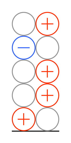
(a)

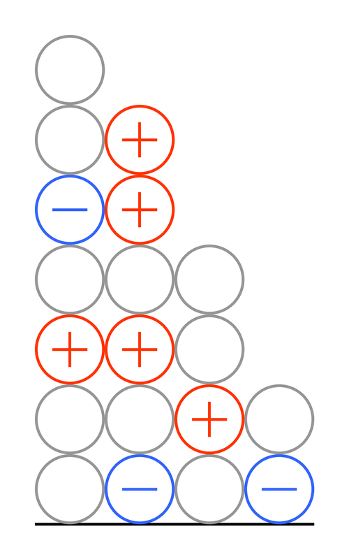
(b)

Figure 2: $ab^{2}a^{-1}b\in\mathbb{F}_{2}$ and $a^{-2}_{2}a^{-1}_{4}a_{3}a_{2}a_{4}a_{1}a_{2}a^{-1}_{1}a^{2}_{2}a^{-1}_{4}\in A_{\Gamma}$

Figure 2 gives a pictorial representation of these pilings. Each list represents a column in the piling.

We now present a function which computes the normal form representative from a piling. For us, this is the shortlex shortest word which represents the piling. We remind the reader that this convention is the opposite ordering for normal forms in [1].

Function: word(p, commuting_elements=[])

Input:

1. $p$ = piling.

2. List of commuting generators.

Output: normal form word which represents the piling $p$.

Example 4.2.

The following is an example of how to use this function for the following piling in $A_{\Gamma}=\langle a,b,c\;|\;ac=ca\rangle$:

p=[[1,0],[0,0,-1],[-1,0]]

w=word(p,[(1,3)])

print(w)

The output is:

[1,-3,-2]

CYCLIC REDUCTION

After constructing pilings from our input words, the next step of the conjugacy algorithm is to cyclically reduce each piling.

Function: cyclically_reduce(p, commuting_elements=[])

Input:

1. $p=$ piling.

2. List of commuting generators.

Output:

1. Cyclically reduced piling.

2. Conjugating element.

Example 5.1.

Let $w=abca^{-1}\in\langle a,b,c\;|\;bc=cb\rangle$. We can compute all possible cyclic reductions on $w$ as follows:

p=piling([1,2,3,-1], 3,[(2,3)])

p_cr=cyclically_reduce(p,[(2,3)])

w=word(p_cr[0],[(2,3)])

print(w, p_cr[1])

The output from this is:

[2,3], [1]

This function is the first example where we output a conjugating element. In this example, when we cyclically reduce $w=a\cdot bc\cdot a^{-1}$ to the word $bc$, we have taken out the conjugating element $a$.

GRAPHS

We remind the reader that for the functions in this section, we need to import the networkx module into Python. This makes working with the defining graph much easier, in particular computing induced subgraphs and connected components.

The next step in the conjugacy algorithm is to compute the non-split factors from a word based on the defining graph. First, we need a method to input our defining graph.

Function: graph_from_edges(N, commuting_edges=[])

Input:

1. $N=$ number of vertices in defining graph.

2. List of commuting generators.

Output: networkx graph, which represents the defining graph.

We recall that in [1], the convention is to add edges for non-commuting vertices. This is precisely what this function does - the output is a graph on $N$ vertices, with edges between vertices $(x,y)$ if and only if $(x,y)$ is not in the list of commuting generators.

Example 6.1.

Let’s compute the defining graph from Equation 1. We input the following:

CGW_Edges = [(1,4), (2,3), (2,4)]

g = graph_from_edges(4, CGW_Edges)

nx.draw(g)

This outputs the following graph:

Figure 3: networkx graph defined in Example 6.1.

Factorising

We now want to build up a function which takes our defining graph $g$ and our input word $w$, and computes the non-split factors related to $w$.

Function: factorise(g, p)

Input:

1. $g=$ networkx graph representing the defining graph of $A_{\Gamma}$.

2. $p=$ piling.

Output: List of subgraphs of $g$, one for each non-split factor of $p$.

This function first checks which columns in the piling contain a 1 or -1 bead (this is the supp_piling() function). From this subset of vertices, we build the induced subgraph, and then return a list of the connected components of this subgraph. Each of these connected components represents the non-split factors.

At this stage, we have extracted each of the subgraphs which correspond to the factors. We now want to extract pilings which represent each factor.

Function: graphs_to_nsfactors(l, w, N, commuting_elements)

Input:

1. $l=$ list of subgraphs representing connected components.

2. $w=$ word representing a group element of $A_{\Gamma}$.

3. $N=$ number of vertices in defining graph.

4. List of commuting generators.

Output: list of the non-split factors from $w$ represented by pilings.

Example 6.2.

We use the example from Figure 4 of [1]. We input the following:

w = [2,3,-4]

CGW_Edges = [(1,4), (2,3), (2,4)]

g = graph_from_edges(4, CGW_Edges)

graphs = factorise(g, piling(w, 4, CGW_Edges))

print(graphs_to_nsfactors(graphs, w, 4, CGW_Edges))

The output is

[[[0], [1], [], []], [[0], [], [1, 0], [0, -1]]]

where the first piling represents the factor $a_{2}$, and the second piling represents the factor $a_{3}a^{-1}_{4}$.

PYRAMIDAL PILINGS

For the final step in the algorithm, we need a function which converts pilings into pyramidal pilings. After this, we need to check when two pyramidal pilings are equal up to cyclic permutation.

Function: pyramidal_decomp(p, commuting_elements=[])

Input:

1. $p=$ non-split piling.

2. List of commuting generators.

Output: factors $p_{0},p_{1}$ as pilings.

It is important to note that the input piling must be non-split, otherwise we cannot achieve a pyramidal piling and the function will run forever.

Example 7.1.

Let’s compute the decomposition in Figure 5 of [1]. We input the following:

CGW_Edges = [(1,4), (2,3), (2,4)]

p = [[0,1,0,-1,0], [0,1,0,1], [0,1,0,0], [-1,0]]

decomp = pyramidal_decomp(p, CGW_Edges)

print(decomp)

The output is then

([[0], [], [0, 1], [-1, 0]], [[1, 0, -1, 0], [0, 1, 0, 1], [0, 0], []])

Function: pyramidal(p, N, commuting_elements=[])

Input:

1. $p=$ non-split cyclically reduced piling.

2. $N=$ number of vertices in defining graph.

3. List of commuting generators.

Output:

1. Pyramidal piling of $p$.

2. Conjugating element.

The pyramidal() function iteratively applies pyramidal_decomp() until the factor $p_{0}$ is empty. Since the only operation we apply on the piling is cyclic permutations, we can add these steps to our conjugating element.

Example 7.2.

Again we take the same example above. Our input is:

CGW_Edges = [(1,4), (2,3), (2,4)]

p = [[0,1,0,-1,0], [0,1,0,1], [0,1,0,0], [-1,0]]

pyr = pyramidal(p, 4, CGW_Edges)

Figure 4 gives the pictorial representation of this pyramidal piling. The conjugating element output in this example is [-4,3,-4].

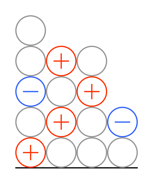
Figure 4: Pyramidal piling.

Function: is_cyclic_permutation(w,v)

Input: Two words $w,v$ representing group elements in $A_{\Gamma}$.
Output: If $w$ is a cyclic permutation of $v$, the function outputs two arguments:

1. True

2. Conjugating element.

Otherwise, return False.

IMPLEMENTATION OF THE CONJUGACY PROBLEM

Simple Cases

If we want to solve the conjugacy problem in either $\mathbb{F}_{n}$ or $\mathbb{Z}^{n}$, the algorithm for implementing the conjugacy problem is more straightforward, and using the is_conjugate() function detailed below is wasteful. Certainly in the latter case, the conjugacy problem is trivial; it is equivalent to checking if two words are equal, which is just a case of comparing the number of occurrences of each letter in the words. For free groups, two cyclically reduced words are conjugate if and only if they are cyclic permutations of each other. Hence one can make a shorter program for free groups by simply using the cyclically_reduce() and is_cyclic_permutation() functions.

For general RAAGs, we now have the necessary functions to implement the conjugacy problem.

Function: is_conjugate(w1, w2, N, commuting_elements=[])

Input:

1. Two words $w_{1},w_{2}$ representing group elements in $A_{\Gamma}$.

2. $N=$ number of vertices in defining graph.

3. List of commuting generators.

Output: If $w_{1}$ is conjugate to $w_{2}$ in $A_{\Gamma}$ then return:

1. True

2. Conjugating element $x$ such that $w_{1}=x^{-1}w_{2}x$.

Otherwise, return False.

We note that when computing the conjugating element, we find a reduced word $x$ which represents an element which conjugates $w_{1}$ to $w_{2}$.

Appendix A The ‘draw piling’ Function

The representation of pilings as a list of lists of 1s, -1s and 0s is not very readable in the Python interpreter. For small pilings it is tolerable, but for larger ones the draw_piling() function is useful.

draw_piling() can take a total of nine arguments, however only the first one, which is the piling to be drawn, is needed. The function returns nothing, but by default it will show a picture of the piling in a new window, as well as save a PNG file of it.

The following table lists all the arguments of the draw_piling() function and what they do:

Argument	Type	Description
piling	Piling	The (mandatory) piling to draw.
scale	Float	The scale to draw the piling at. Default is 100.0.
plus_colour	Colour	The colour to draw the ‘$+$’ beads. Default is red.
zero_colour	Colour	The colour to draw the ‘$0$’ beads. Default is grey.
minus_colour	Colour	The colour to draw the ‘$-$’ beads. Default is blue.
anti_aliasing	Integer	The super-sampling resolution for anti-aliasing.
		Only allows positive integers. Default is 4.
filename	String	The filename to save the piling as. Default is "piling.png".
show	Boolean	Whether to show the piling in a window. Default is True.
save	Boolean	Whether to save the piling. Default is True.

Appendix B Solution to the Word Problem

With the tools that pilings.py provides, it is not hard to solve the Word Problem in any given RAAG. The following code defines a function that decides if a given word is equal to the identity:

def identity(w, N, commuting_elements=[]):

p=piling(w, N, commuting_elements)#generate reduced piling

reduced_w=word(p, commuting_elements)#read off reduced word

return(reduced_w==[])#return whether it equals the identity

The following code defines a function that decides if two given words are equal in a given RAAG:

def equal(w1, w2, N, commuting_elements=[]):

#generate reduced pilings

p1=piling(w1, N, commuting_elements)

p2=piling(w2, N, commuting_elements)

#read off reduced words

reduced_w1=word(p1, commuting_elements)

reduced_w2=word(p2, commuting_elements)

#return whether they are equal

return(reduced_w1==reduced_w2)

SCHOOL OF MATHEMATICAL AND COMPUTER SCIENCES, HERIOT-WATT UNIVERSITY, EDINBURGH, SCOTLAND, EH14 4AS

Email address: ggc2000@hw.ac.uk, mj74@hw.ac.uk

References

- [1] John Crisp, Eddy Godelle, and Bert Wiest. The conjugacy problem in subgroups of right-angled artin groups. Journal of Topology, 2:442–460, 2009.
- [2] Dan Margalit and Matt Clay, editors. Office Hours with a Geometric Group Theorist. Princeton University Press, 2017.