Causal Inference for Continuous Multiple Time Point Interventions

Abstract

There are limited options to estimate the treatment effects of variables which are continuous and measured at multiple time points, particularly if the true dose-response curve should be estimated as closely as possible. However, these situations may be of relevance: in pharmacology, one may be interested in how outcomes of people living with -and treated for- HIV, such as viral failure, would vary for time-varying interventions such as different drug concentration trajectories. A challenge for doing causal inference with continuous interventions is that the positivity assumption is typically violated. To address positivity violations, we develop projection functions, which reweigh and redefine the estimand of interest based on functions of the conditional support for the respective interventions. With these functions, we obtain the desired dose-response curve in areas of enough support, and otherwise a meaningful estimand that does not require the positivity assumption. We develop $g$-computation type plug-in estimators for this case. Those are contrasted with g-computation estimators which are applied to continuous interventions without specifically addressing positivity violations, which we propose to be presented with diagnostics. The ideas are illustrated with longitudinal data from HIV positive children treated with an efavirenz-based regimen as part of the CHAPAS-3 trial, which enrolled children $<13$ years in Zambia/Uganda. Simulations show in which situations a standard g-computation approach is appropriate, and in which it leads to bias and how the proposed weighted estimation approach then recovers the alternative estimand of interest.

1 Introduction

Causal inference for multiple time-point interventions has received considerable attention in the literature over the past few years: if the intervention of interest is binary, popular estimation approaches include inverse probability of treatment weighting approaches (IPTW) [1], g-computation estimators [2, 3] and longitudinal targeted maximum likelihood estimators (LTMLE) [4], among others. For IPTW, the treatment and censoring mechanisms need to be estimated at each time point, parametric g-computation requires fitting of both the outcome and confounder mechanisms, sequential g-computation is based on the iterated outcome regressions only, and LTMLE needs models for the outcome, censoring, and treatment mechanisms, iteratively at each point in time. All of those methods are relatively well-understood and have been successfully applied in different fields (e.g., in [5, 6, 7, 8, 9, 10]).

However, suggestions on how to estimate treatment effects of variables that are continuous and measured at multiple time points are limited. This may, however, be of interest to construct causal dose-response curves (CDRC). For example, in pharmacoepidemiology, one may be interested in how counterfactual outcomes vary for different dosing strategies for a particular drug, see Section 2.

Early work on continuous interventions includes the seminal paper of Robins, Hernán and Brumback [1] on inverse probability weighting of marginal structural models (MSMs). For a single time point, this requires the estimation of stabilized weights based on the conditional density of the treatment, given the confounders. This density may be estimated with parametric regression models, such as linear regression models. The MSM, describing the dose-response relationship (i.e., the CDRC), can then be obtained using weighted regression. The suggested approach can also be used for the longitudinal case, where stabilized weights can be constructed easily, and one may work with a working model where, for example, the effect of cumulative dose over all time points on the response is estimated.

There are several other suggestions for the point treatment case (i.e., a single time point): for example, the use of the generalized propensity score (GPS) is often advocated in the literature [11]. Similar to the MSM approach described above, both the conditional density of the treatment, given the confounders, and the dose-response relationship have to be specified and estimated. Instead of using stabilized weights, the GPS is included in the dose-response model as a covariate. To reduce the risk of bias due to model mis-specification, it has been suggested to incorporate machine learning (ML) in the estimation process [12]. However, when combining GPS and ML approaches, there is no guarantee for valid inference, i.e., related confidence intervals may not achieve nominal coverage [4]. Doubly robust (DR) approaches allow the integration of ML while retaining valid inference. As such, the DR-estimator proposed by Kennedy et al. [13] is a viable alternative to both MSM and GPS approaches. It does not rely on the correct specification of parametric models and can incorporate general machine learning approaches. As with other, similar, approaches [14] both the treatment and outcome mechanisms need to be modelled. Then a pseudo-outcome based on those two estimated nuisance functions is constructed, and put into relationship with the continuous intervention using kernel smoothing. Further angles in the point treatment case are given in the literature [15, 16, 17, 18].

There are fewer suggestions as to how to estimate CDRCs for multiple time point interventions. As indicated above, one could work with inverse probability weighting of marginal structural models and specify a parametric dose-response curve. Alternatively, one may favour the definition of the causal parameter as a projection of the true CDRC onto a specified working model [19]. Both approaches have the disadvantage that, with mis-specification of the dose-response relationship or an inappropriate working model, the postulated curve may be far away from the true CDRC. Moreover, the threat of practical positivity violations is even more severe in the longitudinal setup, and working with inverse densities – which can be volatile – remains a serious concern [20]. It has thus been suggested in the literature to avoid these issues by changing the scientific question of interest, if meaningful, and to work with alternative definitions of causal effects.

For example, Young et al. [21] consider so-called modified treatment policies, where treatment effects are allowed to be stochastic and depend on the natural value of treatment, defined as the treatment value that would have been observed at time $t$, had the intervention been discontinued right before $t$. A similar approach relates to using representative interventions, which are stochastic interventions that maintain a continuous treatment within a pre-specified range [22]. Diaz et al. [23] present four estimators for longitudinal modified treatment policies (LMTPs), based on IPTW, g-computation and doubly robust considerations. These estimators are implemented in an R-package (lmtp). An advantage of those approaches is that the usual positivity assumption can be substantially relaxed. Moreover, the proposed framework is very general, applicable to longitudinal and survival settings, and one is not forced to make arbitrary parametric assumptions if the doubly robust estimators are employed. It also avoids estimation of conditional densities as it recasts the problem at hand as a classification procedure for the density ratio of the post-intervention and natural treatment densities. A disadvantage of the approach is that it does not aim at estimating the CDRC, which may, however, relate to the research question of interest, see Section 2 below.

In this paper, we are interested in counterfactual outcomes after intervening on a continuous intervention (such as drug concentration) at multiple time points. For example, we may be interested in the probability of viral suppression after one year of follow-up, had HIV-positive children had a fixed concentration level of efavirenz during this year. In this example, it would be desirable to estimate the true CDRC as closely as possible, to understand and visualize the underlying biological mechanism and decide what preferred target concentrations should be. This comes with several challenges: most importantly, violations of the positivity assumption are to be expected with continuous multiple time-point interventions. If this is the case, estimands that are related to modified treatment policies or stochastic interventions, as discussed above, would elegantly tackle the positivity violation problem, but redefine the question of interest. In pharmacoepidemiology and other fields this may be not ideal, as interpretations of the true CDRC are of considerable clinical interest, for example to determine appropriate drug target concentrations.

We propose g-computation based approaches to estimate and visualize causal dose-response curves. This is an obvious suggestion in our setting because developing a standard doubly robust estimator, e.g. a targeted maximum likelihood estimator, is not possible as the CDRC is not a pathwise-differentiable parameter; and developing non-standard doubly robust estimators is not straightforward in a multiple time-point setting. Our suggested approach has two angles:

1. As a first step, we simply consider computing counterfactual outcomes for multiple values of the continuous intervention (at each time point) using standard parametric and sequential g-computation. We evaluate with simulation studies where this “naive” estimation strategy can be successful and useful, and where not; and which diagnostics may be helpful in judging its reliability. To our knowledge, this standard approach has not been evaluated in the literature yet.

2. We then define regions of low support through low values of the conditional treatment density, evaluated at the intervention trajectories of interest. Our proposal is to redefine the estimand of interest (i.e., the CDRC) only in those regions, based on suitable weight functions. Such an approach entails a compromise between identifiability and interpretability: it is a tradeoff between estimating the CDRC as closely as possible [as in i)], at the risk of bias due to positivity violations and minimizing the risk of bias due to positivity violations, at the cost of redefining the estimand in regions of low support. We develop a g-computation based plug-in estimator for this weighted approach.

We introduce the motivating question in Section 2, followed by the theoretical framework in Section 3. After presenting our extensive Monte-Carlo simulations (Section 4), we analyze the illustrative data example in Section 5. We conclude in Section 6.

2 Motivating Example

Our motivating data example comes from CHAPAS-3, an open-label, parallel-group, randomised trial (CHAPAS-3) [24]. Children with HIV (aged 1 month to 13 years), from four different treatment centres (one in Zambia, three in Uganda) were assigned to receive antiretroviral therapy (ART) with fixed-dose combination tablets: random allocation related to the nucleoside reverse transcriptase inhibitors (NRTIs) abacavir, stavudine or zidovudine (i.e. the first drug), which was given together with lamivudine (second drug) and the third drug, a nonnucleoside reverse transcriptase inhibitor, either nevirapine or efavirenz (NNRTI, third drug, chosen at discretion of the treating physician). The primary endpoint were adverse events, both clinical (grade 2/3/4) and laboratory (confirmed grade 3, or any grade 4).

Several substudies of the trial explored pharmacokinetic aspects of the nonnucleoside reverse transcriptase inhibitors (i.e. efavirenz and nevirapine), in particular the relationship between the respective drug concentrations and elevated viral load, i.e. viral failure [25, 26]. In those studies, individual pharmacokinetic (PK) measures such as plasma concentration 12 hours after dose were determined through population PK modeling and associations with viral failure were explored using the Cox proportional hazards model, showing lower levels of failure with increased drug concentrations. The reason to focus on the concentration of the NNRTI drugs is because i) they are expected to be responsible for most of the viral suppression and ii) the action of NRTI drugs is intercellularly, which means that the measured plasma concentrations are not necessarily relevant.

As highlighted in similar studies [27, 28, 29], a refined hypothesis relates to understanding the biologic mechanism between drug concentration and viral outcomes: to determine optimal target concentrations that can be translated into recommended doses, possibly depending on patients’ metabolizing status. This equates to asking about the causal effect of drug concentration, measured and controlled over a particular time period, on viral failure. Understanding the true (nonlinear) intervention-outcome relationship is crucial as both too low and too high concentrations could result in negative outcomes. However, drawing a particular CDRC is challenging for the following reasons: (i) the form of the curve should be flexible and as close as possible to the truth; (ii) there exist time-dependent confounders (e.g., adherence, weight) that are themselves affected by prior concentration levels, making regression an invalid method for causal effect estimation [30]; (iii) with long follow-up and moderate sample size, positivity violations are an issue of concern that have to be addressed.

We illustrate our concepts using the data from Bienczak et al. [25]. More details on the data analysis are given in Section 5.

3 Framework

3.1 Notation

We consider a longitudinal data setup where at each time point $t$, $t=0,1,\ldots,T$, we measure the outcome $Y_{t}$, a continuous intervention $A_{t}$ and covariates $L^{j}_{t}$, $j=1,\ldots,q$. We denote $\mathbf{L_{0}}=\{L^{1}_{0},\ldots,L^{q_{0}}_{0}\}$ as “baseline variables” and $\mathbf{L}_{t}=\{L^{1}_{t},\ldots,L^{q}_{t}\}$ as follow-up variables, with $q,q_{0}\in\mathbb{N}$. The intervention and covariate histories of a unit $i$ (up to and including time $t$) are $\bar{A}_{t,i}=(A_{0,i},\ldots,A_{t,i})$ and $\bar{L}^{s}_{t,i}=(L^{s}_{0,i},\ldots,L^{s}_{t,i})$, $s=1,...,q$, $i=1,\ldots,n$, respectively. The observed data structure is

$$O=(\mathbf{L}_{0},A_{0},Y_{0},\mathbf{L}_{1},A_{1},Y_{1},\ldots,\mathbf{L}_{T},A_{T},Y_{T})\stackrel{{\scriptstyle iid}}{{\sim}}P_{0}\,.$$

We are interested in the counterfactual outcome $Y_{t,i}^{\bar{a}_{t}}$ that would have been observed at time $t$ if unit $i$ had received, possibly contrary to the fact, the intervention history $\bar{A}_{t,i}=\bar{a}_{t}$, $a_{t,i}\in\mathbb{R}$. For a given intervention $\bar{A}_{t,i}=\bar{a}_{t}$, the counterfactual covariates are denoted as $\bar{\mathbf{L}}_{t,i}^{\bar{a}_{t}}$. We use $\mathbf{H}_{t}$ to denote the history of all data up to before $A_{t}$.

3.2 Estimands

3.2.1 Estimands for one time point

In order to illustrate the ideas, we first consider a simple example with only one time point where $O=(\mathbf{L},A,Y)$. Assume $\mathbf{L}$ has density $p_{0}(\mathbf{l})$ with respect to some dominating measure $\nu(\mathbf{l})$. In this case, the general dose-response curve $m:a\mapsto E(Y^{a})$ can be identified [13] as

$$m(a) =E_{\mathbf{L}}[E(Y^{a}\mid A=a,\mathbf{L})]=E_{\mathbf{L}}[E(Y\mid A=a,\mathbf{L})]$$

$$=\int E(Y\mid A=a,\mathbf{L}=\mathbf{l})p_{0}(\mathbf{l})d\nu(\mathbf{l})\,,$$ (1)

where the first equality follows by the law of iterated expectation, the assumption that $Y^{a}$ is independent of $A$ conditional on $\mathbf{L}$ (conditional exchangeability) and positivity. The second equality follows because $Y^{a}=Y$ in the event of $A=a$ (consistency).

An example of such a curve for a particular interval $[a_{\min},a_{\max}]$ is given in Figure 1a.

This quantity is undefined if the conditional density function $g(a\mid\mathbf{l})$ is such that $\inf_{{a}\in{\mathcal{A}}}g({a}\mid\mathbf{l})=0$ for values $l$ where $p_{0}(\mathbf{l})>0$ and $\mathcal{A}$ denotes the set of all possible interventions $A=a$. Thus, it is usually required that $\inf_{{a}\in{\mathcal{A}}}g({a}\mid\mathbf{l})>0$ almost everywhere, the so-called strong positivity assumption. In this paper, we address violations of the positivity assumption through a redefinition of the estimand of interest, where we replace the marginal distribution function of $\mathbf{L}$ in (1) by a user-given distribution function. That is, we instead estimate

$$m_{w}(a)=\int E(Y\mid A=a,\mathbf{L}=\mathbf{l})w(a,\mathbf{l})p_{0}(\mathbf{l})d\nu(\mathbf{l})$$ (2)

for some weight function $w(a,\mathbf{l})$. This is essentially a weighted average of the conditional dose-response curve $E(E(Y^{a}\mid\mathbf{L})\,w(a,\mathbf{L}))$. To illustrate the construction of this function, consider two extreme cases: $w(a,\mathbf{l})=1$, and $w(a,\mathbf{l})=g(a\mid\mathbf{l})/g(a)$, where $g(a)$ is the marginal density of $A$. Under the first case, we have $m_{w}(a)=m(a)$, which is equal to the dose-response curve whenever the positivity assumption holds. Under $w(a,\mathbf{l})=g(a\mid\mathbf{l})/g(a)$, we have $m_{w}(a)=E(Y\mid A=a)$, which is not a causal quantity (unless exchangeability is assumed) but it does not require the positivity assumption. We therefore propose to use a function $w(a,\mathbf{l})$ such that $w(a,\mathbf{l})\to 1$ in areas of $\mathcal{A}$ that have good support, and $w(a,\mathbf{l})\to g(a\mid\mathbf{l})/g(a)$ in areas of $\mathcal{A}$ such that $g(a\mid\mathbf{l})$ is close to zero. Thus, one possible function to use is

$$w_{1}(a,\mathbf{l})=\begin{cases}1&\text{ if }{g(a\mid\mathbf{l})}>c\\ \frac{g(a\mid l)}{g(a)}&\text{ otherwise. }\\ \end{cases}$$ (3)

Using (3) yields the desired dose-response curve under enough support, and otherwise $E(Y|A=a)$. Note that both $m(a)$ and $m_{w}(a)$ are undefined outside the support region of $A$. For instance, in the motivating data example the CDRC is undefined for negative concentration values and biologically implausible concentration values of $>40$ mg/L.

(a) CDRC for one time point

(b) Linear weight function

(c) Possible CDRC visualization
– if intervention values are constant over time

(d) Possible CDRC visualization
– if intervention values vary over time (or for survival data)

Figure 1: Considerations for causal dose-response curves (CDRCs)

Estimands under different weight functions
There are alternative weight functions that assign a weight of $1$ under enough support, i.e when values of functions of $g(a,\mathbf{l})$ are large enough, and assign weights based on some density of $A$ and/or $\mathbf{L}$ otherwise:

$$w(a,\mathbf{l})=\begin{cases}1&\text{ if }{h_{1}(g(a|\mathbf{l}))}>c\,,\\ h_{2}(g(a,\mathbf{l}))&\text{ if }{h_{1}(g(a|\mathbf{l}))}\leq c\,.\end{cases}$$

For example, consider the following weight choice which is illustrated in Figure 1b:

$$w_{2}(a,\mathbf{l})=\left\{\begin{array}[]{ll}1&\quad\mbox{for}\quad h_{1}(g(a\mid\mathbf{l}))>c_{2}\\ c_{1}+\frac{1-c_{1}}{c_{2}}\times h_{2}(g(a\mid\mathbf{l}))&\quad\mbox{for}\quad h_{1}(g(a\mid\mathbf{l}))\leq c_{2}\end{array}\right.\,.$$ (6)

An interesting choice for both $h_{1}$ and $h_{2}$ is the expectation (function) with respect to $\mathbf{L}$: with this choice, we achieve that if the marginal support with respect to $a$ is not large enough, the marginal support itself is used as the weight function. Such a weight choice has been motivated in the context of estimands that are defined through parameters in a marginal structural working model for (continuous summaries of) longitudinal binary interventions [31]. Then, for any $0\leq c_{1},c_{2}\leq 1$, the estimand entails a compromise between the CDRC and a weighted CDRC, weighted by marginal support for the respective interventions: for the latter, greater weight is given to interventions with greater marginal support; and the more support there is for each possible intervention choice, the estimand will be closer to the CDRC. This entails a pragmatic compromise between identifiability and interpretability. A similar tradeoff is achieved by using other weight choices that are monotone with respect to the density function $g(a\mid\mathbf{l})$, for example

$$w_{3}(a,\mathbf{l})=\begin{cases}1&\text{ if }{g(a\mid\mathbf{l})}>c_{2}\\ \frac{g(a\mid\mathbf{l})}{g(a\mid\mathbf{l})+c_{1}g(a)}&\text{ if }g(a\mid\mathbf{l})\leq c_{2}\\ \end{cases}\,,$$

$$w_{4}(a,\mathbf{l})=\begin{cases}1&\text{ if }{g(a\mid\mathbf{l})}>c_{2}\\ 1-\exp\left\{-c_{1}\frac{g(a\mid\mathbf{l})}{g(a)}\right\}&\text{ if }g(a\mid\mathbf{l})\leq c_{2}\\ \end{cases}\,.$$

3.2.2 Estimands for Multiple Time Points

If there are multiple time points, we may typically be interested in how the counterfactual outcome at time $t$ would change for all possible (or a set of selected) intervention trajectories – possibly conditional on some baseline variables. That is, we seek to estimate the causal dose-response curve

$$m_{t}:\bar{a}_{t}\mapsto E(Y^{\bar{a}_{t}}_{t}|\mathbf{L_{0}}^{\ast})\quad\quad\forall t\in\mathcal{T}\,\text{and}\,\mathbf{L_{0}}^{\ast}\subseteq\mathbf{L_{0}}\,,$$ (7)

where $\mathcal{T}=\{0,1,\ldots,T\}$, $\bar{a}_{t}\in\bar{\mathcal{A}}_{t}$, and $\bar{\mathcal{A}}_{t}$ denotes either i) the set of all strategies $\bar{a}_{t}=(a_{0},\ldots,a_{t})$ for which the curve is defined or ii) a relevant subset of interest. If we are interested in (7), we can identify the estimand through the sequential g-formula (also known as the iterated conditional expectation representation [3]) under sequential conditional exchangeability, consistency and positivity [32] as follows (we use $\mathbf{L_{0}}^{\ast}=\emptyset$ for ease of illustration):

$$\mathbb{E}(Y_{t}^{\bar{a}_{t}}) = \mathbb{E}(\,\ldots\mathbb{E}(\,\mathbb{E}(Y_{t}|\bar{{A}}_{t}=\bar{a}_{t},\mathbf{\bar{L}}_{t})|\bar{{A}}_{t-1}=\bar{a}_{t-1},\mathbf{\bar{L}}_{t-1}\,)\ldots|{A}_{0}={a}_{0},\mathbf{{L}}_{0}\,)\,)\,.$$ (8)

In the above expression $\bar{Y}_{t-1}$ is part of $\mathbf{\bar{L}}_{t}$. Because $A_{t}$ is continuous, positivity requires that for the respective conditional density functions, we have $P(g(a_{t}\mid\mathbf{H}_{t}))>0\quad\forall t$. More formally, we require

$$\inf_{{a}_{t}\in{\mathcal{A}}_{t}}g({a}_{t}\mid\mathbf{h}_{t})>0\quad\text{whenever}\quad p_{0}(\mathbf{l}_{t}\mid A_{t-1}=a_{t-1},\mathbf{H}_{t-1}=\mathbf{h}_{t-1})>0\quad\forall t\in\mathcal{T}\,.$$ (9)

This assumption may be relaxed under additional parametric modeling assumptions and the set $\mathcal{A}_{t}$ may be reduced based on the scientific question of interest; see Section 3.3.2 for a thorough discussion. Consistency in the multiple time-point case is the requirement that $Y^{\bar{a}_{t}}_{t}=Y_{t}$ if $\bar{A}_{t}=\bar{a}_{t}$ and $\bar{\mathbf{L}}_{t}^{\bar{a}_{t}}=\bar{\mathbf{L}}_{t}$ if $\bar{A}_{t-1}=\bar{a}_{t-1}$. With sequential conditional exchangeability we require the counterfactual outcome under the assigned treatment trajectory to be independent of the actually assigned treatment at time $t$, given the past: $Y^{\bar{a}_{t}}_{t}\coprod A_{t}|\bar{H}_{t}$ for $t=0,\ldots,T$.

To link the above longitudinal g-computation formula to our proposals for one time point, it may be written in terms of the following recursion. Let $\tilde{m}_{t+1}=Y_{t}$. For $s=t,\ldots,0$ recursively define

$$\tilde{m}_{s}:(a_{s},\mathbf{h}_{s})\mapsto\int\tilde{m}_{s+1}(a_{s+1},\mathbf{h}_{s+1})\,dP_{0}(\mathbf{l}_{s+1}\mid A_{s}=a_{s},\mathbf{H}_{s}=\mathbf{h}_{s})\,,$$ (10)

where $\int\tilde{m}_{s+1}(a_{s+1},\mathbf{h}_{s+1})\,dP_{0}(\mathbf{l}_{s+1}\mid A_{s}=a_{s},\mathbf{H}_{s}=\mathbf{h}_{s})$ = $E(\tilde{m}_{s+1}(a_{s+1},\mathbf{H}_{s+1})|A_{s}=a_{s},\mathbf{H}_{s}=\mathbf{h}_{s})$.

Then, the counterfactual mean outcome $E(Y_{t}^{\bar{a}_{t}})$ is identified as $\mathbb{E}(\tilde{m}_{0}(A_{0},H_{0}))$, which follows from the re-expression of (10) in terms of (8) by recursively evaluating the integral. The above recursive integral is well defined only if the positivity assumption (9) is met. As before, we propose to address violations of the positivity assumption by estimating the following quantity instead:

$$\tilde{m}_{w,s}:(a_{s},\mathbf{h}_{s})\mapsto\int\tilde{m}_{s+1}(a_{s+1},\mathbf{h}_{s+1})w_{s}(a_{s+1},\mathbf{h}_{s+1})dP_{0}(\mathbf{l}_{s+1}\mid A_{s}=a_{s},\mathbf{H}_{s}=\mathbf{h}_{s})\,.$$ (11)

As before, if the weight function $w_{s}(a_{s+1},\mathbf{h}_{s+1})$ is equal to one, the above expression can be used to define the actual CDRC (7) through recursive evaluation of (11). If, however, the weight function is equal to

$$w_{s}(a_{s+1},\mathbf{h}_{s+1})=\frac{g_{s}(a_{s+1}\mid\mathbf{h}_{s+1})}{g_{s}(a_{s+1}\mid a_{s},\mathbf{h}_{s})},$$ (12)

then the estimand becomes

$$\tilde{m}_{w,s}:(a_{s},\mathbf{h}_{s})\mapsto\int\tilde{m}_{s+1}(a_{s+1},\,\mathbf{h}_{s+1})dP_{0}(\mathbf{l}_{s+1}\mid A_{s+1}=a_{s+1},A_{s}=a_{s},\mathbf{H}_{s}=\mathbf{h}_{s})$$ (13)

by application of Bayes’ rule. Intuitively, the above quantity does not remove confounding of the relation between $A_{s+1}$ and $Y_{s+1}$, because it conditions on $A_{s+1}=a_{s+1}$ rather than fixing (i.e., intervening on) $A_{s+1}=a_{s+1}$. However, the above expression does not require the positivity assumption to be well defined, as motivated further below.

For the longitudinal case, we follow a strategy similar to that considered for the single time-point case, and consider a compromise between satisfying the positivity assumption and adjusting for confounding. This compromise can be achieved by using weight functions that are $1$ in areas of good support, and are equal to (12) in areas of poor support. If the denominator in (12) is very small, we may want to compromise further:

$$w_{s,1}(a_{s+1},\mathbf{h}_{s+1},c)=\begin{cases}1&\text{ if }g_{s}(a_{s+1}\mid\mathbf{h}_{s+1})>c\,,\\ \frac{g_{s}(a_{s+1}\mid\mathbf{h}_{s+1})}{g_{s}(a_{s+1}\mid a_{s},\mathbf{h}_{s})}&\text{ if }g_{s}(a_{s+1}\mid\mathbf{h}_{s+1})\leq c\text{ and }g_{s}(a_{s+1}\mid a_{s},\mathbf{h}_{s})>c\,,\\[2.0pt] \frac{g_{s}(a_{s+1}\mid\mathbf{h}_{s+1})}{g_{s}(a_{s+1}\mid a_{s-1},\mathbf{h}_{s-1})}&\text{ if }g_{s}(a_{s+1}\mid\mathbf{h}_{s+1})\leq c\text{ and }g_{s}(a_{s+1}\mid a_{s},\mathbf{h}_{s})\leq c\\ &\text{ and }g_{s}(a_{s+1}\mid a_{s-1},\mathbf{h}_{s-1})>c\,,\\ \vdots&\vdots\\[2.0pt] \frac{g_{s}(a_{s+1}\mid\mathbf{h}_{s+1})}{g_{s}(a_{s+1})}&\text{ otherwise }.\\ \end{cases}$$ (14)

Using the weights (14) in (11) returns the CDRC if there is enough conditional support in terms of $g_{s}(a_{s+1}\mid\mathbf{h}_{s+1})>c$ for all $s$; if there is not enough conditional support and the weight denominator $g_{s}(a_{s+1}\mid a_{s},\mathbf{h}_{s})$ is greater than $c$ for all time points, then the estimand equates to $E(Y_{t}|A_{t}=a_{t},\ldots,A_{0}=a_{0})$; this follows from recursively applying (13) for $s=t,\ldots,0$. Thus, no positivity assumption as defined in (9) is required for identification because whenever a positivity violation is present in terms of $g_{s}(a_{s+1}\mid\mathbf{h}_{s+1})\leq c$ for a given $a_{s+1}$ and $\mathbf{h}_{s+1}$ (that is, either a structural violation or a practical violation at estimation stage) the weights (14) redefine the estimand in a way such that the assumption is not needed. Note that, as in the single time point case, the CDRC is undefined outside the support region of $\bar{A}_{t}$. If there is not enough conditional support and the weight denominator is smaller than $c$, the estimand entails an additional compromise. A different compromise is achieved if the weights are applied only at selected time points: the estimand then implies conditioning on $A_{s}=a_{s}$ for those time points, but intervening with $A_{s}=a_{s}$ on the others. However, it is difficult to think of situations where such an estimand would be meaningful.

If we now reexpress our target quantity (11) in terms of an iterated conditional expectation representation, we get:

$$\mathbb{E}_{w_{1}}(Y_{t}^{\bar{a}_{t}}) = \mathbb{E}_{w_{1,0}}(\,\ldots\mathbb{E}_{w_{1,t-1}}(\,\mathbb{E}_{w_{1,t}}(Y_{t}|\bar{{A}}_{t}=\bar{a}_{t},\mathbf{\bar{L}}_{t})|\bar{{A}}_{t-1}=\bar{a}_{t-1},\mathbf{\bar{L}}_{t-1}\,)\ldots|{A}_{0}={a}_{0},\mathbf{{L}}_{0}\,)\,)\,,$$ (15)

where we define $\mathbb{E}_{w_{1,t}}(Y_{t}|\bar{A}_{t}=\bar{a}_{t},\mathbf{\bar{L}}_{t})=\mathbb{E}(w_{1,t}Y_{t}|\bar{A}_{t}=\bar{a}_{t},\mathbf{\bar{L}}_{t})$. This can be rewritten as

$$\mathbb{E}_{w_{1}}(Y_{t}^{\bar{a}_{t}}) = \int_{\mathbf{\bar{l}}\in\mathbf{\bar{L}}_{t}}\left\{\begin{aligned} &\mathbb{E}(w_{1,t}Y_{t}|\bar{\mathbf{A}}_{t}=\bar{a}_{t},\mathbf{\bar{L}}_{t}=\mathbf{\bar{l}}_{t})\times\\ &\prod_{r=0}^{t}\begin{array}[]{l}f(\mathbf{l}_{r}|\bar{\mathbf{A}}_{r-1}=\bar{a}_{r-1},\mathbf{\bar{L}}_{r-1}=\mathbf{\bar{l}}_{r-1})\end{array}\end{aligned}\right\}\,d\mathbf{\bar{l}}\,,$$ (16)

where the second term in (16) is

$$\prod_{s=1}^{q-1} f(l_{r}^{s}|\bar{\mathbf{A}}_{r-1}=\bar{a}_{r-1},\mathbf{\bar{L}}_{r-1}=\mathbf{\bar{l}}_{r-1},L_{r}^{1}=l_{r}^{1},\ldots,L_{r}^{s-1}=l_{r}^{s-1})$$

$$\times f(w_{1,r}Y_{r}|\bar{\mathbf{A}}_{r}=\bar{a}_{r},\mathbf{\bar{L}}_{r}=\mathbf{\bar{l}}_{r})\,.$$

The equality follows from the knowledge that iterated nested expectation representations of the g-formula can be reexpressed as a traditional g-formula factorization because both representations essentially standardize with respect to the post intervention distribution of the time-dependent confounders [3, 6, 33]. In our case, the outcome is $w_{1,t}Y_{t}$.

Interpretation of the weighted estimand
The weighted CDRC can be interpreted as follows: those units which have a covariate trajectory that makes the intervention value of interest at $t$ not unlikely to occur (under the desired intervention before $t$), receive the intervention at $t$; all other units get different interventions that produce, on average, outcomes as we would expect among those who actually follow the intervention trajectory of interest (if the denominator $g_{t}(a_{t+1}\mid a_{t},\mathbf{h}_{t})$ is well-defined). Informally speaking, we calculate the CDRC in regions of enough support and stick to the actual research question, but make use of the marginal associations otherwise, if possible.

As a practical illustration for this interpretation, consider our motivating study: if, given the covariate and intervention history, it seems possible for a child to have a concentration level of $a$ mg/l, then we do indeed calculate the counterfactual outcome under $a$. For some patients however, it may be unlikely (or even biologically impossible!) to actually observe this concentration level: for example, children who are adherent to their drug regimen and got an appropriate drug dose prescribed, but are slow metabolizers will likely never be able to have very low concentration values. In this case, we do not consider the intervention to be feasible and rather let those patients have individual concentration levels which generate outcomes that are typical for children with $a$ mg/l. In short, we calculate the probability of failure at time $t$ if the concentration level is set at $a$ for all patients where this seems “feasible”, and otherwise to individual concentration trajectories that produce “typical” outcomes with $a$ mg/l.

The interpretation of this weighted dose-response curve seems somewhat tricky because the interventions for some units are only defined in terms of the outcomes they produce; note however that this approach has the advantages that i) compared to a naive approach it does not require the positivity assumption, and ii) compared to LMTP’s it sticks to the actual research question as close as “possible”. There are of course other options to define interventions under positivity violations with different interpretations; we will describe such approaches, along with their advantages and disadvantages, in a separate paper.

Summarizing the multiple time-point CDRC graphically
Sometimes, we may want to visualize the CDRC graphically, e.g. by plotting $m_{t}(\bar{a}_{t})$ for each $t$ (and stratified by $\mathbf{L_{0}}^{\ast}$, if meaningful) if the set of strategies is restricted to those that always assign the same value at each time point, see Figure 1c for an illustration. Alternatively, we may opt to plot the CDRC as a function of $t$, for some selected strategies $\bar{a}_{t}$, see Figure 1d. This may be useful if intervention values change over time, or for survival settings.

3.3 Estimation

To estimate the weighted dose-response curve, we can rely on plug-in estimation of either (15) or (16). That is, we use either a parametric or sequential g-formula type of approach where the (iterated) outcome is multiplied with the respective weight at each time point. As the weighted outcome may possibly have a skewed, complex distribution (depending on the weights), we advocate for the use of (15) as a basis for estimation. This is because estimating the expectation only may then be easier than estimating the whole conditional distribution. In many applications, a data-adaptive estimation approach may be a good choice for modeling the expectation of the weighted outcome. The algorithm in Table 1 presents the detailed steps for a substitution estimator of (15).

Table 1: Algorithm for estimating the weighted CDRC at time $t$

Step 0a:	Define a set of interventions $\bar{\mathcal{A}}_{t}$, with $|\bar{\mathcal{A}}_{t}|=n_{a}$ and $\bar{A}^{(j)}_{t}$ is the $j^{\text{th}}$ element of $\bar{\mathcal{A}}_{t}$, $j=1,\ldots,n_{a}$.
Step 0b:	Set $\tilde{Y}_{t}=Y_{t}$.
For $\mathbf{s=t,\ldots,1}$:
Step 1a:	Estimate the conditional density $g(A_{s}|\mathbf{H}_{s})$.
Step 1b:	Estimate the conditional density $g(A_{s}|A_{s-1},\mathbf{H}_{s-1})$.
Step 2:	Set $a_{s}=a_{s}^{(1)}$, where $a_{s}^{(1)}$ is the $s^{\text{th}}$ element of intervention $\bar{A}^{(1)}_{t}\in\bar{\mathcal{A}}_{t}$.
Step 3a:	Plug in $a_{s}^{(1)}$ into the estimated densities from step 1, to calculate $\hat{g}(a_{s}^{(1)}|\mathbf{h}_{s})$ and $\hat{g}(a_{s}^{(1)}|a_{s-1}^{(1)},\mathbf{h}_{s-1})$.
Step 3b:	Calculate the weights $w_{s}(a_{s}^{(1)},c)$ from (14) based on the estimates from 3a.
	If $\hat{g}(a_{s}^{(1)}|a_{s-1}^{(1)},\mathbf{h}_{s-1})\leq c$, estimate $g(a_{s}^{(1)}|a_{s^{\ast}}^{(1)},\mathbf{h}_{s^{\ast}})$ as required by the definition of (14) for $s^{\ast}=s-2,\ldots,0$.
Step 4:	Estimate $\mathbb{E}(w_{s}(a_{s}^{(1)},c)\,\tilde{Y}_{s}|{A}_{s},\mathbf{H}_{s})$.
Step 5:	Predict $\tilde{Y}_{s-1}=\hat{\mathbb{E}}(\hat{w}_{s}(a_{s}^{(1)},c)\,\tilde{Y}_{s}|\bar{A}_{s}=\bar{a}_{s}^{(1)},\mathbf{l}_{s})$ based on the fitted model from step 4 and the given intervention $\bar{a}_{s}^{(1)}$.
For $\mathbf{t=0}$:
Step 1a:	Estimate the conditional density $g(A_{0}|\mathbf{L}_{0})$.
Step 1b:	Estimate the conditional density $g(A_{0})$.
Step 2:	Set $a_{0}=a_{0}^{(1)}$.
Step 3a:	Calculate $\hat{g}(a_{0}^{(1)}|\mathbf{l}_{0})$ and $\hat{g}(a_{0}^{(1)})$.
Step 3b:	Calculate the weights $w_{0}(a_{0}^{(1)},c)$. If $\hat{g}(a_{0}^{(1)})\leq c$, then ${m}_{w,t}(\bar{a}_{t}^{(1)},c)$ is undefined.
Step 4:	Estimate $\mathbb{E}(w_{0}(a_{0}^{(1)},c)\,\tilde{Y}_{0}|{A}_{0},\mathbf{L}_{0})$.
Step 5:	Calculate $\hat{m}_{w,t}(\bar{a}_{t}^{(1)},c)=\hat{\mathbb{E}}_{w(c)}(Y_{t}^{\bar{a}_{t}^{(1)}})=(\sum_{i}w_{0,i})^{-1}(\hat{w}_{0}(a_{0}^{(1)},c)^{\text{T}}\tilde{Y}_{0})$; that is, obtain the estimate of the weighted CDRC at $\bar{a}_{t}^{(1)}$ through calculating the weighted mean.
Then:
Step 6:	Repeat steps 2-5 for the other interventions $\bar{A}_{t}^{(j)}$, $j=2,\ldots,n_{a}$. This yields an estimate of the desired dose-response curve (7) at $t$.
Time-to-event data:
Possible changes, to recover $E(Y_{t}^{\bar{C}_{t}=0}|A_{t}=a_{t},\ldots,A_{0}=a_{0})$ if there is not enough support for $\bar{A}^{(j)}_{t}$.
Step 1a/b:	Estimate the densities among those uncensored, and without prior event ($C_{t}=0,Y_{t-1}=0$).
Step 2:	Also, set $c_{t}=0$ (we only describe the setting where we intervene on censoring).
Step 4:	Fit the model for the weighted outcome among those uncensored and without prior event,
	that is, estimate $\mathbb{E}(w_{t}(a_{t}^{(1)},c)\,\tilde{Y}_{t}|\bar{A}_{t},C_{t}=0,Y_{t-1}=0,\mathbf{H}_{t})$.
Step 5:	Additionally, set $\tilde{Y}_{t-1,i}=1$, if $Y_{t-2,i}=1$.

For the estimates of the weighted curve to be consistent, both the expected weighted (iterated) outcomes and the weights need to be estimated consistently.

Note that for $t=0$, we suggest to calculate a weighted mean, instead of estimating the weighted expected outcome data-adaptively. This is because the former is typically more stable when $Y_{0}$ follows some standard distribution, but $w_{0}$ does not. It is a valid strategy as standardizing with respect to the pre-intervention variables $L_{0}$ and then calculating the weighted mean of the outcome is identical to standardizing the weighted outcome with respect to $L_{0}$, and then calculating the mean. Another option for $t=0$ is to facilitate step 6 before step 5 and then create a stacked dataset of the counterfactual outcomes for all intervention values $a_{0}$, and then fit a weighted regression of $Y_{0}$ on $A_{0}$, based on the stacked weight vectors. The fitted model can then be used to predict the expected outcome under all $a_{0}$. This strategy is however not explored further in this paper.

3.3.1 Multiple Interventions and Censoring

So far, we have described the case of 1 intervention variable $A_{t}$ per time point. Of course, it is possible to employ the proposed methodology for multiple intervention variables $\mathbf{A}_{t}=(A_{t,1},A_{t,2},\ldots,A_{t,p})$. In this case, one simply has to estimate the conditional densities for all those intervention variables, and taking their product, at each time point. This follows from replacing (12) with ${g_{s}(\mathbf{a}_{s+1}\mid\mathbf{h}_{s+1})}/{g_{s}(\mathbf{a}_{s+1}\mid\mathbf{a}_{s},\mathbf{h}_{s})}$, and then factorizing the joint intervention distribution based on the assumed time ordering of $(L_{s},A_{s,1},A_{s,2},$ $\ldots,A_{s,p},Y_{s})$. Intervention variables may include censoring variables: we may, for instance, construct CDRC’s under the intervention of no censoring. A possible option to apply the proposed methodology is then to recover the estimand $E(Y_{t}^{\bar{C}_{t}=0}|A_{t}=a_{t},\ldots,A_{0}=a_{0})$ if there is not enough conditional support for the intervention strategy of interest. Table 1 lists the required modifications of the estimation procedure, based on a time-ordering of $(L_{s},A_{s,1},A_{s,2},\ldots,A_{s,p},C_{s},Y_{s})$, $s=0,\ldots,t$. An alternative estimand to recover would be $E(Y_{t}|C_{t}=c_{t},A_{t}=a_{t},\ldots C_{0}=c_{0},A_{0}=a_{0})$. For this, one would require estimating the conditional censoring mechanisms in steps 1a and 1b too. There are however many subtleties and dangers related to the interpretation and estimation of CDRC’s under censoring, and possibly competing events; for example, conditioning on the censoring indicators may lead to collider bias, intervening the on censoring mechanisms to direct effect estimands [34], identification assumptions need to be refined and generic time-orderings where treatment variables are separated by different blocks of confounders may lead to more iterated expectations that have to be fitted. Those details go beyond the scope of this paper.

3.3.2 On Practical Violations of the Positivity Assumption and Diagnostics

The positivity assumption, as defined in (9), is a strong requirement. It is however important to highlight that in many practical applications one may not be interested in all possible intervention histories, but only in a (very restricted) subset of intervention trajectories – and thus only in some parts of the full CDRC. For instance, in the data example, we are only interested in positive drug concentrations ($\leq$6 mg/L) and in intervention strategies where the concentration is constant over time; complex concentration trajectories, where values increase and decrease, and more generally fluctuate over time do not relate to the most meaningful scientific estimands in this case. It is therefore likely that we require the positivity assumption to only hold for particular areas of the conditional treatment densities; and that we can evaluate those areas as a diagnostic tool. Let $\bar{\mathcal{A}}_{t}$ be the set of interventions of interest, with $|\bar{\mathcal{A}}_{t}|=n_{a}$ being small and $\bar{A}^{(j)}_{t}=(a_{0}^{(j)},\ldots,a_{t}^{(j)})$ is the $j^{\text{th}}$ element of $\bar{\mathcal{A}}_{t}$, $j=1,\ldots,n_{a}$. Suppose the intervention values at $t$ are already ordered such that $a_{t}^{(1)}<a_{t}^{(2)}<\ldots<a_{t}^{(n_{a})}$. Then we can approximate the relevant parts of conditional treatment densities with a binning strategy in the sense that we calculate

$$P\left(a_{t}^{(j)}\in\left[a_{t}^{(j)}-\frac{1}{2}(a_{t}^{(j)}-a_{t}^{(j-1)});\,a_{t}^{(j)}+\frac{1}{2}(a_{t}^{(j)}-a_{t}^{(j+1)}\right)\,\middle|\,\right.$$

$$\left.\quad\quad\quad\quad\quad\bar{a}_{t-1}^{(j)}\in\left[a_{t-1}^{(j)}-\frac{1}{2}(a_{t-1}^{(j)}-a_{t-1}^{(j-1)});\,a_{t-1}^{(j)}+\frac{1}{2}(a_{t-1}^{(j)}-a_{t-1}^{(j+1)}\right),\bar{l}_{t}\right)\,;$$ (17)

that is, we want to estimate the probability to approximately observe the intervention value $a_{t}^{(j)}$ under strategy $j$, given that one has followed the same strategy of interest $j$ so far (until $t-1$), and irrespective of the covariate history. Alternatively, instead of defining the bin widths through the intervention values of interest, we may calculate them data-adaptively [35]. Estimating the mean of those probabilites over all observed $\bar{l}_{t}$ in a particular data set serves as diagnostic tool to measure the support for each rule $j$, at each time point. Note that we can relax the positivity assumption further for standard g-computation analyses, if we are willing to assume that the parametric modeling assumptions at the estimation stage are complex enough to extrapolate into regions of low support [36]. We propose to estimate (3.3.2) with standard regression techniques, and present a summary of those probabilites as a rough measure of support for each intervention trajectory of interest. With this, one may judge where standard g-computation estimates are more reliable, and where they may be best complemented with weighted CDRCs using the projection functions presented above.

An alternative diagnostic approach is to report the proportion of weights which are unequal to 1; that is, to estimate the conditional treatment density either with (3.3.2), or differently, and evaluate which proportion is below the threshold $c$, for each intervention trajectory of interest. This approach is presented in the data analysis, in Figure 4.

4 Monte-Carlo Simulations

In this section, we evaluate the proposed methods in three different simulation settings. Simulation 1 considers a very simple setting, as a basic reference for all approaches presented. In simulation 2, a survival setting is considered, to explore the stability of standard, unweighted g-computation in more sophisticated setups. The third simulation is complex, and inspired by the data-generating process of the data analysis. It serves as the most realistic setup for all method evaluations.

Data Generating Processes & Estimands

Simulation 1: We simulated both a binary and normally distributed confounder, a continuous (normally distributed) intervention and a normally distributed outcome – for 3 time points and a sample size of $n=10.000$. The exact model specifications are given in Appendix B.1. The intervention strategies of interest comprised intervention values in the interval $[2,11]$ which were constant over time; that is, $\bar{\mathcal{A}}_{t}^{1}=\{(2,2,2),\ldots,(11,11,11)\}$ . The primary estimand $\psi^{1}$ is the CDRC (7) for $t=1,2,3$, $\mathbf{L}_{0}^{\ast}=\emptyset$ and all $\bar{a}_{t}\in\bar{\mathcal{A}}^{1}_{t}$. The secondary estimand $\psi^{1}_{w}$ is the weighted CDRC defined through (11), with the weights (14), for the same intervention strategies.

Simulation 2: We simulated a continuous (normally distributed) intervention, two covariates (one of which is a confounder), an event outcome and a censoring indicator – for 5 time points and varying sample sizes of $n_{1}=500,n_{2}=1.000,n_{3}=10.000$ and $n_{4}=50.000$. The exact model specifications are given in Appendix B.2. The intervention strategies of interest comprised intervention values in the interval $[-7,13]$ which were constant over time; that is, $\bar{\mathcal{A}}_{t}^{2}=\{(-7,-7,-7,-7,-7),\ldots,(13,13,13,13,13)\}$. The estimand $\psi^{2}$ is the CDRC (7) for $t=1,2,3,4,5$, $\mathbf{L}_{0}^{\ast}=\emptyset$, all $\bar{a}_{t}\in\bar{\mathcal{A}}^{2}_{t}$ and under no censoring ($\bar{c}_{t}=(0,\ldots,0)$).

Simulation 3: We simulated data inspired by the data generating process of the data example outlined in Sections 2 and 5 as well as Figure 3. The continuous intervention refers to drug concentration (of evavirenz), modeled through a truncated normal distribution. The binary outcome of interest is viral failure. Time-varying confounders, affected by prior interventions, are weight and adherence. Other variables include co-morbidities and drug dose (time-varying) we well as sex, genotype, age and NRTI regimen. We considered 5 clinic visits and a sample size of $n=1.000$. The exact model specifications are given in Appendix B.3. The intervention strategies of interest comprised concentration values in the interval $[0,10]$ which were constant over time; that is, $\bar{\mathcal{A}}_{t}^{3}=\{(0,0,0,0,0),\ldots,(10,10,10,10,10)\}$. The primary estimand $\psi_{3}$ is the CDRC (7) for $t=1,2,3,4,5$, $\mathbf{L}_{0}^{\ast}=\emptyset$ and all $\bar{a}_{t}\in\bar{\mathcal{A}}^{3}_{t}$. The secondary estimand $\psi^{3}_{w}$ is the weighted CDRC (11) with the weights (14) for the same intervention strategies.

Estimation & Evaluation

All simulations were evaluated based on the results of $\mathcal{R}=1.000$ simulation runs. We evaluated the bias of estimating $\psi^{1},\psi^{2}$ and $\psi^{3}$ with standard parametric g-computation with respect to the true CDRC. In simulations 1 and 3 model specification for $g$-computation was based on variable screening with LASSO, simulation 2 explored the idealized setting of using correct model specifications. We further evaluated the bias of the estimated weighted CDRC with the true weighted CDRC, for $c=1$; i.e. we looked whether $E(Y_{t}|A_{t}=a_{t},\ldots,A_{0}=a_{0})$ could be recovered for every intervention strategy of interest. Estimation was based on the algorithm of Table 1. The density estimates, which are required for estimating the weights, were based on both appropriate parametric regression models (that is, linear regression) and binning the continuous intervention into intervals; a computationally more sophisticated data-adaptive approach for density estimation is considered in Section 5. We then compared the estimated CDRC and weighted CDRC ($c=1$) with other weighted CDRC’s where $c=0.01$ and $c=0.001$. To estimate the iterated conditional expectations of the weighted outcome, we used super learning, i.e. a data adaptive approach [4]. Our learner sets included different generalized linear (additive) regression models (with penalized splines, and optionally interactions), multivariate adaptive regression splines, LASSO estimates and regression trees – after prior variable screening with LASSO and Cramer’s V [37]. Lastly, we visualize the conditional support of all considered intervention strategies, in all simulations, as suggested in (3.3.2).

Results

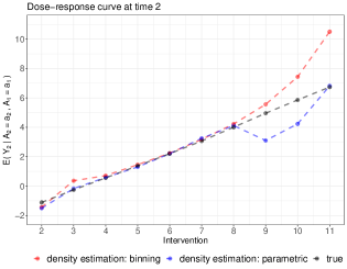
(a) Simulation 1: weighted CDRC, $c=1$, $t=2$

(b) Simulation 2: true and estimated CDRC at $t=2$

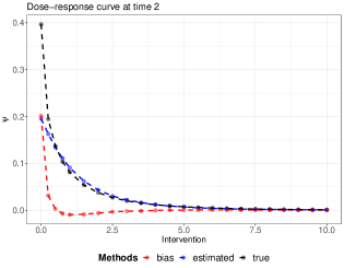
(c) Simulation 3: true and estimated CDRC at $t=2$

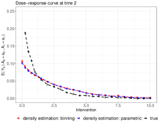
(d) Simulation 1: weighted CDRC, $c=1$, $t=2$

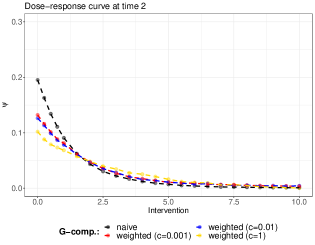
(e) Simulation 3: CDRC’s, $t=2$, $c=0.001,0.01,1$

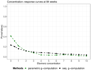
(f) Data analysis: estimated CDRC

Figure 5: Additional simulation and analysis results

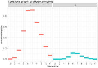
(a) Simulation 1

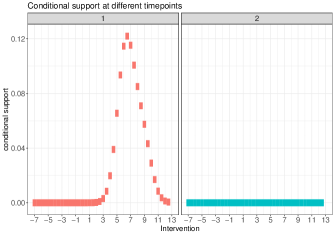
(b) Simulation 2

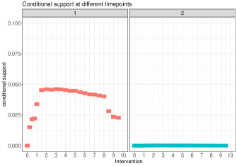
(c) Simulation 3

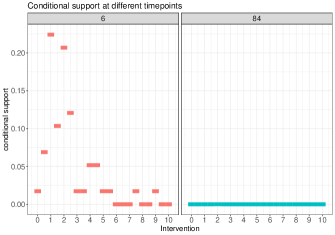
(d) Data Analysis

Figure 6: Conditional support for intervention strategies of interest, for both the simulation settings and the data analysis.

The results of the simulations are summarized in Figures 2, 5 and 6.

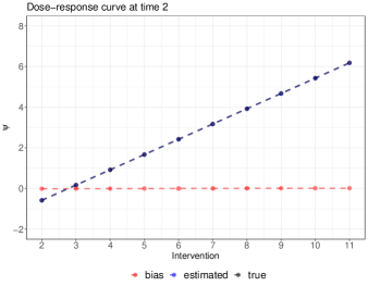
(a) Simulation 1: true and estimated CDRC at $t=2$

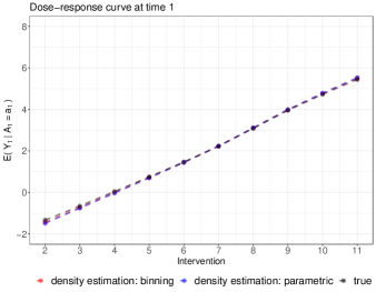
(b) Simulation 1: weighted CDRC, $c=1$, $t=1$

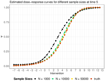
(c) Simulation 2: true and estimated CDRC at $t=5$

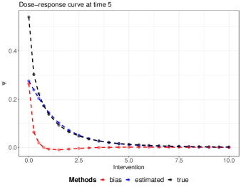
(d) Simulation 3: true and estimated CDRC at $t=5$

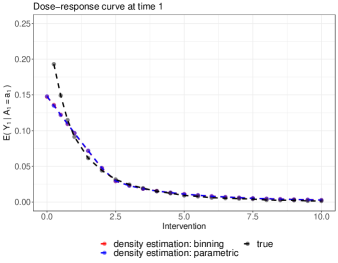
(e) Simulation 3: weighted CDRC, $c=1$, $t=1$

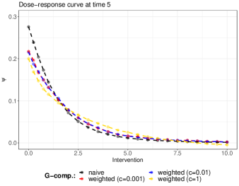
(f) Simulation 3: CDRC’s, $t=5$, $c=0.001,0.01,1$

Figure 2: Results of the Monte-Carlo simulations

In simulation 1, applying standard g-computation to the continuous intervention led to approximately unbiased estimates for all intervention values, through all time points (Figure 2a); and independent of the level of support (Figure 6a). The weighted CDRC, with $c=1$, recovered the association $E(Y_{1}|A_{1}=a_{1})$ perfectly for the first time point, independent of the density estimation strategy (Figure 2b). For later time points, some bias can be observed in regions of lower support (i.e., for intervention values between $9$ and $11$), see Figure 5a.

Simulation 2 shows a setting in which g-computation estimates for the CDRC are not always unbiased, despite correct model specifications! Figure 2c visualizes this finding for the fifth time point: it can be seen that a sample size of $\geq$ 10.000 is needed for approximately unbiased estimation of the CDRC over the range of all intervention strategies. Note, however, that for some time points lower sample sizes are sufficient to guarantee unbiased estimation (Figure 5b).

The most sophisticated simulation setting 3 reveals some more features of the proposed methods. First, we can see that in areas of lowest support, towards concentration values close to zero, there is relevant bias of a standard g-computation analysis (Figure 2d); whereas in areas of reasonable to good support the CDRC estimates are approximately unbiased. The weighted CDRC with $c=1$ can recover the associations $E(Y_{t}|A_{t}=a_{t},\ldots,A_{1}=a_{1})$ for intervention values $\geq 1$, but there is some bias as the most critical area close to zero is approached, independent of the method used for estimating the weights (Figure 2e, and also Figure 5d). Both Figure 2f and Figure 5e highlight the behaviour of the weighted CDRC for $c=0.01$ and $c=0.001$: it can be clearly seen that the curves represent a compromise between the CDRC and the association represented by the weighted CDRC (with $c=1$). Evaluating the results for intervention values of zero, shows that weighting the curve in areas of low support yields to a compromise that moves the CDRC away from the estimated high probabilities of viral failure to more moderate values informed by the observed association. Knowledge of this behaviour may be informative for the data analysis below.

5 Data Analysis

We now illustrate the ideas based on the data from Bienczak et al. [25], introduced in Section 2. We consider the trial visits at $t=0,6,36,48,60,84$ weeks of $125$ children on an efavirenz-based treatment regime. The intervention of interest is efavirenz mid-dose interval concentration ($A_{t}$), defined as plasma concentration (in $mg/L$) 12 hours after dose; the outcome is viral failure ($Y_{t}$, defined as $>100$ copies/mL). Measured baseline variables, which we included in the analysis, are $\mathbf{L_{0}}=\{\text{sex, genotype, age, the nucleoside reverse}$ transcriptase $\text{inhib\-itors drug (NRTI), weight}\}$. Genoytpe refers to the metabolism status (slow, intermediate, extensive) related to the single nucleotide polymorphisms in the CYP2B6 gene, which is relevant for metabolizing evafirenz and directly affects its concentration in the body. Measured follow-up variables are $\mathbf{L}_{t}=\{\text{weight, adherence (measured through memory caps, MEMS), dose}\}$.

The assumed data generating process is visualized in the DAG in Figure 3, and explained in more detail in Appendix C. Briefly, both weight and adherence are time-dependent confounders, potentially affected by prior concentration trajectories, which are needed for identification of the CDRC.

Figure 3: Directed Acyclic graph for the data analysis. The intervention variable is shown in green (efavirenz concentration), the outcome in blue (viral load at the end of follow-up). Unmeasured variables are colored in grey. Both MEMS and weight are time-dependent confounders which are affected by prior treatment nodes.

Our target estimands are the CDRC (7) and the weighted CDRC (11) at $t=84$ weeks. The intervention strategies of interest are $\bar{\mathcal{A}}_{t}=\{(0,0,0,0),\ldots,(6,6,6,6)\}$.

The analysis illustrates the ideas based on a complete case analysis of all measured variables represented in the DAG ($n=58$), but excluding dose (not needed for identification) and MEMS (due to the high proportion of missingness).

We estimated the CDRC both with sequential and parametric g-computation using the intervention strategies $\bar{\mathcal{A}}_{t}$. The estimation of the weighted CDRC followed the algorithm of Table 1. The conditional treatment densities, which are needed for the construction of the weights, were estimated both parametrically based on the implied distributions from linear models (for concentrations under 5 $mg/L$) and with highly-adaptive LASSO conditional density estimation (for concentrations $\geq 5$ $mg/L$) [38, 39]. This is because the density in the lower concentration regions were approximately normally distributed, but more complex for higher values.

The conditional expectation of the weighted outcome (Step 4 of the algorithm) was estimated data-adaptively with super learning using the following learning algorithms: the highly adaptive LASSO, multivariate adaptive regression splines, generalized linear models (also with interactions), generalized additive models as well as the mean and median. Prior variable screening, which was essential given the small sample size, was based on both the LASSO and Cramer’s $V$ .

We estimated the weighted CDRC for $c=0.001,0.01,1$. We also calculate the support of the continuous intervention strategies $\bar{\mathcal{A}}_{t}$ through estimating (3.3.2).

Results

The main results of the analyses are given in Figure 4.

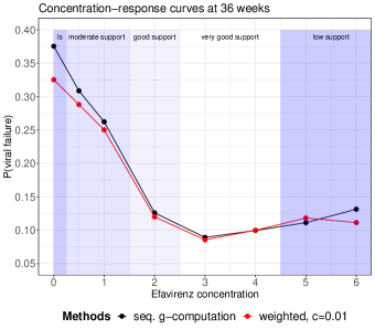
(a) CDRC, weighted CDRC and conditional support, represented through background shading. Support is defined as proportion of weights, which are unequal to 1, see text for details.

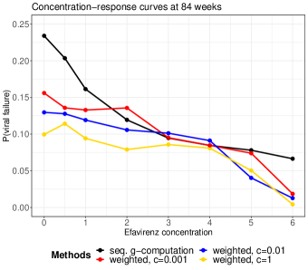
(b) CDRC and weighted CDRC’s

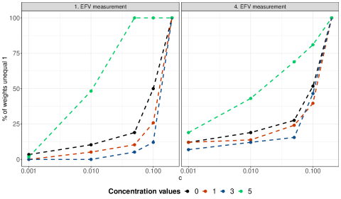
(c) Conditional support and weight behaviour: percentage of weights which are unequal 1, as a function of $c$, visit date and concentration value.

Figure 4: Results of the data analysis

Figures 4a and 4b show that the estimated CDRC (black solid line) suggests higher probabilities of failure with lower concentration values. The curve is steep in the region from $0-2$mg, which is even more pronounced for parametric g-computation when compared to sequential g-computation (Figure 5f).

Both Figures 4a and 6d illustrate the low level of (conditional support) support for extremely small concentration values close to $0$ mg/L and for large concentrations, for both 36 and 84 weeks of follow-up.

Note that in Figure 4a the area shaded in dark blue relates to low conditional support, defined as a proportion $>10$% of weights being unequal than 1; that is, more than 10% of observations having an estimated conditional treatment density $<0.01$ under the respective intervention values. Intermediate, light and no blue background shadings refer to percentages of $7.5-10$%, $5-7.5$% and $<5$%, respectively. More details on how the conditional support defined through weight summaries varies as a function of $c$, visit date and intervention values is illustrated in Figure 4c. It can be seen that with a choice of $c=0.001$ or $c=0.01$, for most patients the actual intervention of interest seems feasible for concentrations values up to below $5$ mg/l; however, concentrations $>5mg/l$ seem often unrealistic and weighting is then used more often.

The weighted curves in Figure 4b are less steep in the crucial areas close to zero and –as in the simulation studies– we observe a tendency of the curves with $c=0.01$ and $c=0.001$ to provide a visual compromise between the CDRC and the estimand recovering the relevant association ($c=1$).

The weighted curves show the probability of failure under different concentration levels, at least if the respective concentration level is likely possible (realistic, probable) to be observed given the patient’s covariate history; for patients where this seems unlikely, patients rather have individual concentrations that lead to outcomes comparable to the patient population with the respective concentration trajectory. For example, if patients are adherent and slow metabolizers, it may be unlikely that they achieve low concentration levels and we do not enforce the intervention of interest. We let these patients rather behave individually in line with otucomes typically seen for low concentration values.

The practical implication is that if we do not want to extrapolate in regions of low support and/or do not consider specific concentration values to be feasible for some patients, the concentration-response curve is flatter. The current lower recommended target concentration limit is 1 $mg/l$, at which we still estimate high failure probabilities under standard g-computation approaches. The weighted curves show us that practically this proportion may however still be somewhat lower, potentially because the features of our patient population may not make low concentrations realistic for everyone.

6 Discussion

We have introduced and evaluated various methods for causal effect estimation with continuous multiple time-point interventions. As an obvious first step, we investigated standard (parametric or sequential) g-formula based approaches for identification and estimation of the actual causal dose-response curve. We emphasized that this has the advantage of sticking to the estimand of interest, but with a relatively strong positivity assumption which will likely be violated in most data analyses. Our simulations were designed to explore how well such a standard approach may extrapolate in sparse data regions and how the approach performs in both simple and complex settings. We found that in simple scenarios the CDRC estimates were approximately unbiased, but that in more complex settings sometimes large sample sizes were needed for good performance and that in regions of very poor support a relatively large bias could be observed. These findings suggest that the toolkit for causal effect estimation with longitudinal continuous interventions should therefore ideally be broader.

A first pragmatic approach to tackle positivity violations is to weigh those estimates of the CDRC down, which are related to interventions that have little or no support in the data. This has already been proposed in the point treatment case for estimands that are defined through parameters in a marginal structural working model (MSM) [36]; or, more generally for MSM parameters which summarize features of longitudinal binary interventions [31]. Suggested choices for the weight function include the marginal support for each intervention. We discussed that this choice, as well similar choices based on the same rationale, entail a compromise between the CDRC and a weighted CDRC in areas of low support, but lack an intuitive interpretation and do not relate to a clear estimand. We have therefore advocated to rather use weights that recover the CDRC if there is enough support, and a meaningful estimand which doesn’t require the positivity assumption otherwise.

Based on this rationale we proposed a weight function which returns the CDRC under enough conditional support, and the crude association between the outcome at time $t$ and the treatment history otherwise. This choice ensures that the estimand is always well-defined and provides a natural compromise between causation and association in areas of low support, where a particular intervention may seem infeasible. Our simulations suggest that the provided estimation algorithm for the weighted CDRC can indeed successfully recover the associational estimand and illustrate the compromise that is practically achieved. As the proposed weights may have skewed distributions, we highlighted the importance of using a data-adaptive estimation approach.

We hope that our manuscript has shown that for continuous multiple time point interventions one has to ultimately make a tradeoff between estimating the CDRC as closely as possible, at the risk of bias due to positivity violations and minimizing the risk of bias due to positivity violations, at the cost of redefining the estimand. If the scientific question of interest allows a redefinition of the estimand in terms of longitudinal modified treatment policies [23] then this may be a great choice. Otherwise, it may be helpful to use g-computation algorithms for continuous interventions, visualize the estimates in appropriate curves, calculate the suggested diagnostics by estimating the conditional support and then estimate the proposed weighted CDRCs as a magnifying glass for the curve’s behaviour in areas of low support.

Our suggestions can be extended in several directions: it may be possible to design different weight functions that keep the spirit of modifying estimands under continuous interventions only in areas of low support; the extent of the compromise, controlled by the tuning parameter $c$, may be chosen data-adaptively and our basic considerations for time-to-event data may be extended to cover more estimands, particular in the presence of competing risks.

Software

All approaches considered in this paper have been implemented in the $R$-packages CICI and CICIplus available at https://cran.r-project.org/web/packages/CICI/index.html and https://github.com/MichaelSchomaker/CICIplus.

Acknowledgements

We are grateful for the support of the CHAPAS-3 trial team, their advise regarding the illustrative data analysis and making their data available to us. We would like to particularly thank David Burger, Sarah Walker, Di Gibb, Andrzej Bienczak and Elizabeth Kaudha. We would also like to acknowledge Daniel Saggau, who has contributed to the data-generating processes of our simulation setups and Igor Stojkov for contributing substantive knowledge to pharmacological angles relevant to the data example. Computations were performed using facilities provided by the University of Cape Town’s ICTS High Performance Computing team. Michael Schomaker is supported by the German Research Foundations (DFG) Heisenberg Programm (grants 465412241 and 465412441).

Appendix A Additional Results

A.1 Simulation and Analysis Results

A.2 Intervention Support

Appendix B Data-Generating Processes

B.1 DGP for Simulation 1

For $t=0$:

$$\text{L}^{1}_{0} \sim \text{B}(p=0.3)$$

$$\text{L}^{2}_{0} \sim \text{N}(\mu=-1+2\times\text{L}^{1}_{0},\,\sigma=1)$$

$$\text{A}_{0} \sim \text{N}(\mu=7+\text{L}^{1}_{0}+0.7\times\text{L}^{2}_{0},\,\sigma=1)$$

$$\text{Y}_{0} \sim \text{N}(\mu=-1+0.5\times\text{A}_{0}+0.5\times\text{L}^{2}_{0},\,\sigma=1)$$

For $t=1,2$:

$$\text{L}^{1}_{t} \sim \text{B}(p=1/(1+\exp(-(-4+\text{L}^{1}_{t-1}+0.15\times\text{L}^{2}_{t-1}+0.15\times\text{A}_{t-1}))))$$

$$\text{L}^{2}_{t} \sim \text{N}(\mu=0.5\times\text{L}^{1}_{t}+0.25\times\text{L}^{2}_{t-1}+0.5\times\text{A}_{t-1},\,\sigma=1)$$

$$\text{A}_{t} \sim \text{N}(\mu=\text{A}_{t-1}+\text{L}^{1}_{t}-0.1\times\text{L}^{2}_{t},\,\sigma=0.5)$$

$$\text{Y}_{t} \sim \text{N}(\mu=-2+0.25\times\text{A}_{t}-0.2\times\text{L}^{1}_{t}+\text{L}^{2}_{t},\,\sigma=0.5)$$

B.2 DGP for Simulation 2

For $t=0$:

$$\text{L}^{1}_{0} \sim \text{B}(p=0.3)$$

$$\text{L}^{2}_{0} \sim \text{N}(\mu=-1+2\times\text{L}^{1}_{0},\,\sigma=1)$$

$$\text{A}_{0} \sim \text{N}(\mu=7+\text{L}^{1}_{0}+0.7\times\text{L}^{2}_{0},\,\sigma=1)$$

$$\text{Y}_{0} \sim \text{B}(p=1/(1+\exp(-(-4+0.2\times\text{A}_{0}+0.5\times\text{L}^{2}_{0}))))$$

For $t=1,2,3,4$:

$$\text{L}^{1}_{t} \sim \text{B}(p=1/(1+\exp(-(-4+\text{L}^{1}_{t-1}+0.15\times\text{L}^{2}_{t-1}+0.15\times\text{A}_{t-1}))))$$

$$\text{L}^{2}_{t} \sim \text{N}(\mu=0.5\times\text{L}^{1}_{t}+0.25\times\text{L}^{2}_{t-1}+0.5\times\text{A}_{t-1},\,\sigma=1)$$

$$\text{A}_{t} \sim \text{N}(\mu=-2+0.5\times\text{A}_{t-1}+0.75\times\text{L}^{1}_{t}+0.35\times\text{L}^{2}_{t},\,\sigma=0.5)$$

$$\text{C}_{t} \sim \text{B}(p=1/(1+\exp(-(-2+0.5\times\text{L}^{1}_{t}+0.2\times\text{A}_{t}))))$$

$$\text{Y}_{t} \sim \text{B}(p=1/(1+\exp(-(-4+0.2\times\text{A}_{t}+0.5\times\text{L}^{2}_{t}))))$$

B.3 DGP for Simulation 3

Both baseline data ($t=0$) and follow-up data ($t=1,\ldots,4$) were created using structural equations using the $R$-package simcausal. The below listed distributions, listed in temporal order, describe the data-generating process. Our baseline data consists of sex, genotype, $\log(\text{age})$, $\log(\text{weight})$ and the respective Nucleoside Reverse Transcriptase Inhibitor (NRTI). Time-varying variables are co-morbidities (CM), dose, efavirenz mid-dose concentration (EFV), elevated viral load (= viral failure, VL) and adherence (measured through memory caps, MEMS), respectively. In addition to Bernoulli ($B$), Multinominal ($MN$) and Normal ($N$) distributions, we also use truncated normal distributions; they are denoted by $N_{[a,a_{1},a_{2},b,b_{1},b_{2}]}$, where $a$ and $b$ are the truncation levels. Values which are smaller than $a$ are replaced by a random draw from a $U(a_{1},a_{2})$ distribution and values greater than $b$ are drawn from a $U(b_{1},b_{2})$ distribution, where $U$ refers to a continuous uniform distribution. For the specified multinomial distributions, probabilities are normalized, if required, such that they add up to 1. The data-generating process reflects the following considerations: more complexity than the first two simulation settings in terms of distribution shape and variety, as well as non-linearities; similarity to the assumed DGP in the data analysis; generation of both areas of poor and good conditional intervention support, such that the proposed weighting scheme can be evaluated in all its breadth.

For $t=0$:

$$\text{Sex}_{0} \sim \text{B}(p=0.5)$$

$$\text{Genotype}_{0} \sim \text{MN}\left(\begin{array}[]{ll}p1=1/(1+\exp(-(-0.103+\text{I}(\text{Sex}_{0}=1)\times 0.223+\text{I}(\text{Sex}_{0}=0)\times 0.173)))\,,\\ p2=1/(1+\exp(-(-0.086+\text{I}(\text{Sex}_{0}=1)\times 0.198+\text{I}(\text{Sex}_{0}=0)\times 0.214)))\,,\\ p3=1/(1+\exp(-(-0.090+\text{I}(\text{Sex}_{0}=1)\times 0.082+\text{I}(\text{Sex}_{0}=0)\times 1.070)))\\ \end{array}\right)$$

$$\text{Age}_{0} \sim N_{[0.693,0.693,1,2.7,2.7,2.8]}(\mu=1.501,\sigma=0.369)$$

$$\text{Weight}_{0} \sim N_{[2.26,2.26,2.67,3.37,3.02,3.37]}(\mu=(1.5+0.2\times\text{Sex}+0.774\times\text{Age})\times 0.94),\sigma=0.369)$$

$$\text{NRTI}_{0} \sim \text{MN}\left(\begin{array}[]{ll}p1=1/(1+\exp(-(-0.006+\text{I}(\text{Age}_{0}>1.4563)\times\text{Age}_{0}\times 0.1735+\text{I}(\text{Age}_{0}\leq 1.4563)\times\text{Age}_{0}\times 0.1570)))\,,\\ p2=1/(1+\exp(-(-0.006+\text{I}(\text{Age}_{0}>1.4563)\times\text{Age}_{0}\times 0.1735+\text{I}(\text{Age}_{0}\leq 1.4563)\times\text{Age}_{0}\times 0.1570)))\,,\\ p3=1/(1+\exp(-(-0.006+\text{I}(\text{Age}_{0}>1.4563)\times\text{Age}_{0}\times 0.1570+\text{I}(\text{Age}_{0}\leq.14563)\times\text{Age}_{0}\times 0.1818)))\\ \end{array}\right)$$

$$\text{CM}_{0} \sim \text{B}(p=0.15)$$

$$\text{Dose}_{0} \sim \text{MN}\left(\begin{array}[]{ll}p1=1/(1+\exp(-(5+\sqrt{(\text{Weight}_{0})}\times 8-\text{Age}_{0}\times 10)))\,,\\ p2=1/(1+\exp(-(4+\sqrt{(\text{Weight}_{0})}\times 8.768-\text{Age}_{0}\times 9.06)))\,,\\ p3=1/(1+\exp(-(3+\sqrt{(\text{Weight}_{0})}\times 6.562-\text{Age}_{0}\times 8.325)))\,,\\ p4=1-(p1+p2+p3)\\ \end{array}\right)$$

$$\text{EFV}_{0} \sim N_{[0.2032,0.2032,0.88,21,8.376,21]}(\mu=-8+\text{Age}_{0}\times 0.1+\text{Genotype}_{0}\times 4.66+\text{Dose}_{0}\times 0.1+$$

$$\text{I}(\text{Genotype}_{0}\leq 2)\times 2.66+\text{I}(\text{Genotype}_{0}=3)\times 4.6,\sigma=4.06)$$

$$\text{VL}_{0} \sim \text{B}(p=1-(1/(1+\exp(-(0.4+1.9\times\sqrt{\text{EFV}_{0}})))))$$

For $t\geq 1$:

$$\text{MEMS}_{t} \sim \text{B}(p=1/(1+\exp(-(0.71+\text{CM}_{t-1}\times 0.31+\text{MEMS}_{t-1}\times\text{I}(t\geq 2)\times 0.31))))$$

$$\text{Weight}_{t} \sim N_{[2.26,2.26,2.473,3.37,3.23.37]}(\mu=\text{Weight}_{t-1}\times 1.04-0.05\times\text{I}(\text{CM}_{t-1}=1),\,\sigma=0.4)$$

$$\text{CM}_{t} \sim \text{B}(p=1-(1/(1+\exp(-(0.5\times\text{I}(\text{CM}_{t-1}=1)+\text{Age}_{0}\times 0.1+\text{Weight}_{t-1}\times 0.1)))))$$

$$\text{Dose}_{t} \sim \text{MN}\left(\begin{array}[]{ll}p1=(1/(1+\exp(-(4+\text{Dose}_{t-1}\times 0.5+\sqrt{\text{Weight}_{t}}\times 4-\text{Age}_{0}\times 10)))\,,\\ p2=(1/(1+\exp(-(-8+\text{Dose}_{t-1}\times 0.5+\sqrt{\text{Weight}_{t}}\times 8.568-\text{Age}_{0}\times 9.06)))\,,\\ p3=(1/(1+\exp(-(20+\text{Dose}_{t-1}\times 0.5+\sqrt{\text{Weight}_{t}}\times 6.562-\text{Age}_{0}\times 18.325)))\,,\\ p4=1-(p1+p2+p3)\\ \end{array}\right)$$

$$\text{EFV}_{t} \sim N_{[0.2032,0.2032,0.88,21.84,8.37,21.84]}(\mu=0.1\times\text{DOSE}_{t}+0.1\times\text{MEMS}_{t}+\text{I}(\text{Genotype}_{0}\leq 2)\times 2.66$$

$$\quad+\text{I}(\text{Genotype}_{0}=3)\times 4.6,\sigma=4.06)$$

$$\text{VL}_{t} \sim \text{B}(p=1-(1/(1+\exp(-(1-0.6\times\text{I}(t=1)-1.2\times\text{I}(t=4)+0.1\times\text{CM}_{t-1}+(2-0.2\times\text{I}(t=3))\times\sqrt{\text{EFV}_{t}})))))$$

Appendix C More on the DAG

The measured efavirenz concentration depends on the following factors: the dose itself (which is recommended to be assigned based on the weight-bands), adherence (without regular drug intake, the concentration becomes lower), and the metabolism characterized in the gene CYP2B6, through the 516G and 983T polymorphisms [40]. Given the short half-life of the drug relative to the measurement interval, no arrow from EFV_t to EFV_t+1 is required. Viral failure is essentially caused if there is not enough drug concentration in the body; and there might be interactions with co-morbidites and co-medications. Sometimes resistance could also lead to viral failure, but this point is less relevant in the data example. Note also that co-morbidities, which are reflected in the DAG, are less frequent in the given data analysis as trial inclusion criteria did not allow children with active infections, treated for tuberculosis and laboratory abnormalities to be enrolled into the study. Both weight and MEMS (=adherence) are assumed to be time-dependent confounders affected by prior treatments (=concentrations). Weight affects the concentration indirectly through the dosing, whereas adherence affects it directly. Adherence itself is affected by prior concentrations, as too high concentration values can cause nightmares and other central nervous system side effects, or strong discomfort, that might affect adherence patterns. Weight is affected from prior concentration trajectories through the pathway of viral load and co-morbidites. Finally, both weight and adherence affect viral outcomes not only through EFV concentrations, but potentially also through co-morbidities such as malnutrition, pneumonia and others.

References

- Robins et al. [2000] J. M. Robins, M. A. Hernan, and B. Brumback. Marginal structural models and causal inference in epidemiology. Epidemiology, 11(5):550–560, 2000.
- Robins [1986] J. Robins. A new approach to causal inference in mortality studies with a sustained exposure period - application to control of the healthy worker survivor effect. Mathematical Modelling, 7(9-12):1393–1512, 1986.
- Bang and Robins [2005] H. Bang and J. M. Robins. Doubly robust estimation in missing data and causal inference models. Biometrics, 64(2):962–972, 2005.
- Van der Laan and Rose [2011] M. Van der Laan and S. Rose. Targeted Learning. Springer, 2011.
- Schnitzer et al. [2014] M. E. Schnitzer, M. J. van der Laan, E. E. Moodie, and R. W. Platt. Effect of breastfeeding on gastrointestinal infection in infants: A targeted maximum likelihood approach for clustered longitudinal data. Annals of Applied Statistics, 8(2):703–725, 2014.
- Schomaker et al. [2019] M. Schomaker, M. A. Luque Fernandez, V. Leroy, and M. A. Davies. Using longitudinal targeted maximum likelihood estimation in complex settings with dynamic interventions. Statistics in Medicine, 38:4888–4911, 2019.
- Baumann et al. [2021] P. Baumann, M. Schomaker, and E. Rossi. Estimating the effect of central bank independence on inflation using longitudinal targeted maximum likelihood estimation. Journal of Causal Inference, 9(1):109–146, 2021.
- Bell-Gorrod et al. [2020] H. Bell-Gorrod, M.P. Fox, A. Boulle, H. Prozesky, R. Wood, F. Tanser, M.A. Davies, and M. Schomaker. The impact of delayed switch to second-line antiretroviral therapy on mortality, depending on failure time definition and CD4 count at failure. American Journal of Epidemiology, 189:811–819, 2020.
- Cain et al. [2016] L. E. Cain, M. S. Saag, M. Petersen, M. T. May, S. M. Ingle, R. Logan, J. M. Robins, S. Abgrall, B. E. Shepherd, S. G. Deeks, M. John Gill, G. Touloumi, G. Vourli, F. Dabis, M. A. Vandenhende, P. Reiss, A. van Sighem, H. Samji, R. S. Hogg, J. Rybniker, C. A. Sabin, S. Jose, J. Del Amo, S. Moreno, B. Rodriguez, A. Cozzi-Lepri, S. L. Boswell, C. Stephan, S. Perez-Hoyos, I. Jarrin, J. L. Guest, A. D’Arminio Monforte, A. Antinori, R. Moore, C. N. Campbell, J. Casabona, L. Meyer, R. Seng, A. N. Phillips, H. C. Bucher, M. Egger, M. J. Mugavero, R. Haubrich, E. H. Geng, A. Olson, J. J. Eron, S. Napravnik, M. M. Kitahata, S. E. Van Rompaey, R. Teira, A. C. Justice, J. P. Tate, D. Costagliola, J. A. Sterne, and M. A. Hernan. Using observational data to emulate a randomized trial of dynamic treatment-switching strategies: an application to antiretroviral therapy. International Journal of Epidemiology, 45(6):2038–2049, 2016.
- Kreif et al. [2017] Noémi Kreif, Linh Tran, Richard Grieve, Bianca De Stavola, Robert C Tasker, and Maya Petersen. Estimating the Comparative Effectiveness of Feeding Interventions in the Pediatric Intensive Care Unit: A Demonstration of Longitudinal Targeted Maximum Likelihood Estimation. American Journal of Epidemiology, 186(12):1370–1379, 2017.
- Hirano and Imbens [2004] Keisuke Hirano and Guido W. Imbens. The Propensity Score with Continuous Treatments, chapter 7, pages 73–84. Wiley, 2004.
- Kreif et al. [2015] Noémi Kreif, Richard Grieve, Iván Díaz, and David Harrison. Evaluation of the effect of a continuous treatment: A machine learning approach with an application to treatment for traumatic brain injury. Health Economics, 24(9):1213–1228, 2015.
- Kennedy et al. [2017] Edward H. Kennedy, Zongming Ma, Matthew McHugh, and Dylan S. Small. Nonparametric methods for doubly robust estimation of continuous treatment effects. Journal of the Royal Statistical Society. Series B, Statistical methodology, 79:1229–1245, 2017.
- Westling et al. [2020] Ted Westling, Peter Gilbert, and Marco Carone. Causal isotonic regression. Journal of the Royal Statistical Society, Series B, 82:719–747, 2020.
- Zhang et al. [2016] Zhiwei Zhang, Jie Zhou, Weihua Cao, and Jun Zhang. Causal inference with a quantitative exposure. Statistical Methods in Medical Research, 25(1):315–335, 2016.
- Galvao and Wang [2015] Antonio F. Galvao and Liang Wang. Uniformly semiparametric efficient estimation of treatment effects with a continuous treatment. Journal of the American Statistical Association, 110(512):1528–1542, 2015.
- VanderWeele et al. [2011] Tyler J. VanderWeele, Yu Chen, and Habibul Ahsan. Inference for causal interactions for continuous exposures under dichotomization. Biometrics, 67(4):1414–1421, 2011.
- Díaz and van der Laan [2013] Iván Díaz and Mark J. van der Laan. Targeted data adaptive estimation of the causal dose–response curve. Journal of Causal Inference, 1(2):171–192, 2013.
- Neugebauer and van der Laan [2007] R. Neugebauer and M. van der Laan. Nonparametric causal effects based on marginal structural models. Journal of Statistical Planning and Inference, 137(2):419–434, 2007.
- Goetgeluk et al. [2008] S. Goetgeluk, S. Vansteelandt, and E. Goetghebeur. Estimation of controlled direct effects. Journal of the Royal Statistical Society Series B-Statistical Methodology, 70:1049–1066, 2008.
- Young et al. [2014] Jessica G. Young, Miguel A. Hernan, and James M. Robins. Identification, estimation and approximation of risk under interventions that depend on the natural value of treatment using observational data. Epidemiologic Methods, 3(1):1–19, 2014.
- Young et al. [2019] Jessica G. Young, Roger W. Logan, James M. Robins, and Miguel A. Hernán. Inverse probability weighted estimation of risk under representative interventions in observational studies. Journal of the American Statistical Association, 114(526):938–947, 2019.
- Díaz et al. [2021] Iván Díaz, Nicholas Williams, Katherine L. Hoffman, and Edward J. Schenck. Non-parametric causal effects based on longitudinal modified treatment policies. Journal of the American Statistical Association, in press, 2021.
- Mulenga et al. [2016] Veronica Mulenga, Victor Musiime, Adeodata Kekitiinwa, Adrian D. Cook, George Abongomera, Julia Kenny, Chisala Chabala, Grace Mirembe, Alice Asiimwe, Ellen Owen-Powell, David Burger, Helen McIlleron, Nigel Klein, Chifumbe Chintu, Margaret J. Thomason, Cissy Kityo, A. Sarah Walker, and Diana Gibb. Abacavir, zidovudine, or stavudine as paediatric tablets for african hiv-infected children (chapas-3): an open-label, parallel-group, randomised controlled trial. The Lancet Infectious Diseases, 16(2):169–79, 2016.
- Bienczak et al. [2016a] Andrzej Bienczak, Paolo Denti, Adrian Cook, Lubbe Wiesner, Veronica Mulenga, Cissy Kityo, Addy Kekitiinwa, Diana M. Gibb, David Burger, A. Sarah Walker, and Helen McIlleron. Plasma efavirenz exposure, sex, and age predict virological response in hiv-infected african children. Journal of Acquired Immune Deficiency Syndromes, 73(2):161–168, 2016a.
- Bienczak et al. [2017] Andrzej Bienczak, Paolo Denti, Adrian Cook, Lubbe Wiesner, Veronica Mulenga, Cissy Kityo, Addy Kekitiinwa, Diana M. Gibb, David Burger, Ann S. Walker, and Helen McIlleron. Determinants of virological outcome and adverse events in african children treated with paediatric nevirapine fixed-dose-combination tablets. AIDS, 31(7):905–915, 2017.
- Moholisa et al. [2014] R. R. Moholisa, M. Schomaker, L. Kuhn, S. Meredith, L. Wiesner, A. Coovadia, R. Strehlau, L. Martens, E. J. Abrams, G. Maartens, and H. McIlleron. Plasma lopinavir concentrations predict virological failure in a cohort of South African children initiating a protease-inhibitor-based regimen. Antiviral Therapy, 19(4), 2014.
- Moholisa et al. [2016] R. R. Moholisa, M. Schomaker, L. Kuhn, S. Castel, L. Wiesner, A. Coovadia, R. Strehlau, F. Patel, F. Pinillos, E. J. Abrams, G. Maartens, and H. McIlleron. Effect of lopinavir and nevirapine concentrations on viral outcomes in protease inhibitor-experienced HIV-infected children. Pediatric Infectious Disease Journal, 35(12):e378–e383, 2016.
- Orrell et al. [2016] Catherine Orrell, Andrzej Bienczak, Karen Cohen, David Bangsberg, Robin Wood, Gary Maartens, and Paolo Denti. Effect of mid-dose efavirenz concentrations and CYP2B6 genotype on viral suppression in patients on first-line antiretroviral therapy. International Journal of Antimicrobial Agents, 47(6):466–472, 2016.
- Hernan and Robins [2020] M. Hernan and J. Robins. Causal inference. Chapman & Hall/CRC, Boca Raton, 2020. URL https://www.hsph.harvard.edu/miguel-hernan/causal-inference-book/.
- Petersen et al. [2014] M. Petersen, J. Schwab, S. Gruber, N. Blaser, M. Schomaker, and M. van der Laan. Targeted maximum likelihood estimation for dynamic and static longitudinal marginal structural working models. Journal of Causal Inference, 2(2):147–185, 2014.
- van der Laan and Gruber [2012] M. J. van der Laan and S. Gruber. Targeted minimum loss based estimation of causal effects of multiple time point interventions. International Journal of Biostatistics, 8(1):article 9, 2012.
- Petersen [2014] M. L. Petersen. Commentary: Applying a causal road map in settings with time-dependent confounding. Epidemiology, 25(6):898–901, 2014.
- Young et al. [2020] J. G. Young, M. J. Stensrud, E. J. T. Tchetgen, and M. A. Hernan. A causal framework for classical statistical estimands in failure-time settings with competing events. Statistics in Medicine, 39(8):1199–1236, 2020.
- Díaz and van der Laan [2011] Iván Díaz and Mark van der Laan. Super learner based conditional density estimation with application to marginal structural models. The International Journal of Biostatistics, 7(1):Article 38, 2011. URL https://doi.org/10.2202/1557-4679.1356.
- Petersen et al. [2012] M. L. Petersen, K. E. Porter, S. Gruber, Y. Wang, and M. J. van der Laan. Diagnosing and responding to violations in the positivity assumption. Statistical Methods in Medical Research, 21(1):31–54, 2012.
- Heumann et al. [2023] C. Heumann, M. Schomaker, and Shalabh. Introduction to Statistics and Data Analysis - With Exercises, Solutions and Applications in R. Springer, Heidelberg, 2023.
- Hejazi et al. [2022a] Nima S Hejazi, David Benkeser, and Mark J van der Laan. haldensify: Highly adaptive lasso conditional density estimation, 2022a. URL https://github.com/nhejazi/haldensify. R package version 0.2.3.
- Hejazi et al. [2022b] Nima S. Hejazi, Mark J. van der Laan, and David Benkeser. ‘haldensify‘: Highly adaptive lasso conditional density estimation in ‘r‘. Journal of Open Source Software, 7(77):4522, 2022b. doi: 10.21105/joss.04522. URL https://doi.org/10.21105/joss.04522.
- Bienczak et al. [2016b] A. Bienczak, A. Cook, L. Wiesner, A. Olagunju, V. Mulenga, C. Kityo, A. Kekitiinwa, A. Owen, A. S. Walker, D. M. Gibb, H. McIlleron, D. Burger, and P. Denti. The impact of genetic polymorphisms on the pharmacokinetics of efavirenz in african children. British Journal of Clinical Pharmacology, 82(1):185–98, 2016b.