Object based Bayesian full-waveform inversion for shear elastography

Abstract. We develop a computational framework to quantify uncertainty in shear elastography imaging of anomalies in tissues. We adopt a Bayesian inference formulation. Given the observed data, a forward model and their uncertainties, we find the posterior probability of parameter fields representing the geometry of the anomalies and their shear moduli. To construct a prior probability, we exploit the topological energies of associated objective functions. We demonstrate the approach on synthetic two dimensional tests with smooth and irregular shapes. Sampling the posterior distribution by Markov Chain Monte Carlo (MCMC) techniques we obtain statistical information on the shear moduli and the geometrical properties of the anomalies. General affine-invariant ensemble MCMC samplers are adequate for shapes characterized by parameter sets of low to moderate dimension. However, MCMC methods are computationally expensive. For simple shapes, we devise a fast optimization scheme to calculate the maximum a posteriori (MAP) estimate representing the most likely parameter values. Then, we approximate the posterior distribution by a Gaussian distribution found by linearization about the MAP point to capture the main mode at a low computational cost.

1 Introduction

Medical imaging is a part of biological imaging that aims to reveal internal structures hidden in tissues by non invasive techniques [33], such as X-ray radiography, magnetic resonance imaging, tomography, echography, ultrasound, endoscopy, elastography, tactile imaging, thermography, nuclear medicine and holography. From the mathematical point of view, they all pose inverse problems that aim to deduce the properties of living tissues from observed signals. The typical framework is as follows. A set of emitters launch waves which interact with the tissue. The resulting wave field is recorded at a grid of receptors and analyzed to infer the structure of the medium. Different imaging techniques differ in the waves employed (electromagnetic, acoustic, thermal, elastic, etc), the arrangement of emitters and receivers, and the medium properties monitored.

Harmless modalities using light [36], sound [46] or elastic [47] beams are particularly interesting due to the absence of secondary effects. Elastography is a relatively new imaging technique that maps the elastic properties of soft tissue [47, 50]. Cancerous tumors will often be stiffer than the surrounding tissue (prostate and breast tumors, for instance), whereas damaged livers are harder than healthy ones [3, 27, 50]. While existing technology [45] can distinguish healthy from unhealthy tissue in specific situations, the study of tissues containing multiple anomalies, tiny tumors or little contrast regions may benefit from the development of more refined mathematical approaches.

Here we develop an object based Bayesian full-waveform inversion framework for soft tissue shear elastography with topological priors. Instead of tracking spatial variations of the elastic constants or the wave speeds within the tissue (as is often done in many geophysical and medical applications, see [3, 20, 22, 40, 47, 51], for instance and references therein), we take an inverse scattering approach [10] and represent localized anomalies in the tissue, such as tumors or fibromas, by objects with distinctive elastic constants immersed in the background tissue [25]. A first advantage of this approach is that anomalies are characterized by a few unknowns defining their parametrization and their elastic properties, which reduces the computational cost. Moreover, studies in other imaging set-ups [7] suggest that localized inhomogeneities may be more precisely captured by looking for abrupt interfaces defining their boundaries, and for material parameter variations within them, than by tracking the spatial variations of material parameter fields everywhere. A second advantage is that we can define misfit functionals in terms of object shapes and then use the associated topological energies to construct sharp priors at low cost. Because of their ability to suppress oscillations in configurations with multiple objects, topological energies are used in deterministic inverse scattering frameworks to find first guesses of scatterers in nondestructuve materials testing [13, 14] and in biological applications [44].

Depending on the expected complexity, one can choose different representations for the boundaries of the anomalies [21, 24, 29, 39]. Here, we consider two types of star-shaped parametrizations that differ in the way the radius is parameterized. The boundary of star-shaped objects is defined by an angle dependent distance function (the radius) along rays in all space directions [4]. We can reproduce smooth shapes approximating the radius by trigonometric polynomials involving just a few parameters [26]. Rougher boundaries are better described by high dimensional radius functions [15]. Both situations are of interest to study anomalies in tissues. Tumors, for instance, can display smooth or irregular contours depending on their stage and nature. We show that we can infer the structure of anomalies in tissues with quantified uncertainty by Markov Chain Monte Carlo (MCMC) sampling of posterior distributions which use priors constructed by topological energy methods and likelihoods defined in terms of the difference of the recorded elastography data and synthetic observations generated numerically for arbitrary anomalies. Affine invariant ensemble samplers [23, 16] work reasonably well when we can approximate the radius function by combinations of trigonometric polynomials. We can also extract basic information on irregular objects defined by higher dimensional radius functions. However, MCMC methods are computationally expensive. For simple shapes, we have also developed fast methods which first optimize to calculate a maximum a posteriori [5, 9] approximation to the anomaly parameters and then sample a linearized approximation of the posterior distribution. The computational cost is much lower, but details on the structure of the posterior distributions, such as multimodality, may be lost.

The paper is organized as follows. Section 2 describes the mathematical model for shear wave imaging in the tissue. Section 3 formulates the Bayesian inversion framework. Section 4 explains how to construct priors for the number of anomalies and their shapes. Section 5 uses ensemble MCMC samplers to solve the Bayesian inverse problem and quantify uncertainty in the solution for relevant configurations characterized by low dimensional parameter sets. Well defined maximum a posteriori (MAP) approximations are identified. Section 6 presents a low cost approach which combines optimization to calculate the MAP point and linearization of the posterior probability about it to quantify uncertainty. Finally, section 7 adapts affine-invariant ensamble sampling methods to infer the structure of high dimensional irregular shapes. A final Appendix contains details on the numerical schemes employed and parameter choices made. Section 8 presents our conclusions.

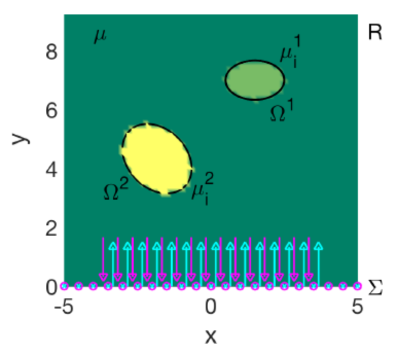
Figure 1: Schematic dimensionless representation of the imaging set-up. The emitters (cyan) generate waves which interact with the medium. The reflected waves are recorded at the receivers (magenta). Emitters and receivers are transducers located at the same position.

2 Physical set-up

Shear elastography tracks variations in the shear modulus $\mu$, which is the property varying more abruptly from healthy to unhealthy tissue, by means of shear waves. Elastic waves in a medium split in shear components (shear S-waves) and compression components (longitudinal P-waves) [31]. Shear waves are adequate for the depths considered in tissues since P-waves travel faster and reach deeper very fast. Moreover, at low frequencies, shear waves are not really affected by attenuation effects in tissues [45] and are governed by standard wave equations.

The imaging set-up is represented in Figure 1. We consider a medium $R\subset\mathbb{R}^{2}$ (the tissue) containing a set of anomalies $\Omega=\cup_{\ell=1}^{L}\Omega^{\ell}$ and locate a set of emitters $\mathbf{x}_{j}$, $j=1,\ldots,J,$ on a part $\Sigma$ of the boundary $\partial R$. The medium has density $\rho$ and elastic constants $\mu$ and $\lambda$, while the anomalies have density $\rho_{\rm i}$ and elastic constants $\mu_{\rm i}$ and $\lambda_{\rm i}$. The emitted waves interact with the medium and the resulting wave field is recorded at a grid of receivers $\mathbf{r}_{k}$, $k=1,\ldots,K$. Emitter and receivers occupy the same region. They can be interspaced, or, in some set-ups, overlap. Here, we will consider they are transducers located at same positions, playing both roles alternatively. Let us formulate the forward problem that governs the dynamics of the wave field in this framework.

To simplify, we consider that the waves emitted by the sources are governed by the scalar wave equation

$$\begin{array}[]{ll}\rho u_{tt}-{\rm div}(\mu\nabla u)=f(t)g(\mathbf{x}),&\mathbf{x}\in R,\;t>0,\\[4.30554pt] u(\mathbf{x},0)=0,u_{t}(\mathbf{x},0)=0,&\mathbf{x}\in R,\end{array}$$ (3)

where

$$\rho(\mathbf{x})=\left\{\begin{array}[]{ll}\rho,&\mathbf{x}\in R\setminus\overline{\Omega},\\ \rho_{\rm i}^{\ell},&\mathbf{x}\in\Omega^{\ell},\;\ell=1,\ldots,L,\end{array}\right.$$

$$\mu(\mathbf{x})=\left\{\begin{array}[]{ll}\mu,&\mathbf{x}\in R\setminus\overline{\Omega},\\ \mu_{\rm i}^{\ell},&\mathbf{x}\in\Omega^{\ell},\ell=1,\ldots,L,\end{array}\right.$$

with local wave speed $\sqrt{\mu\over\rho}$ in the healthy tissue and $\sqrt{\mu_{\rm i}^{\ell}\over\rho_{\rm i}^{\ell}}$ inside each anomaly $\Omega^{\ell}.$ In tissues, we have $\rho_{\rm i}\sim\rho$. We assume that the emitters $\mathbf{x}_{j}$, $j=1,\ldots,J,$ induce source terms of the form $f(t)g_{j}(\mathbf{x}-\mathbf{x}_{j})$, where $g_{j}$ are smooth functions of narrow support about $0$ that we sum to obtain $g(\mathbf{x})$. We represent the function $f(t)$ by a Ricker wavelet $f(t)=f_{0}(1-2\pi^{2}f_{M}^{2}t^{2})e^{-\pi^{2}f_{M}^{2}t^{2}}$ with peak frequency $f_{M}$. The time it takes to move from the initial positive maximum to the negative minimum is $T_{D}={\sqrt{6}\over 2\pi f_{M}}.$ After that it approaches zero.

A whole organ $R$ can be represented by a domain with zero normal derivative at its physical boundary $\partial R$

$$\displaystyle{\partial u\over\partial\mathbf{n}}=0\quad\mbox{\rm on }\,\,\partial R.$$ (6)

Equations (3)-(6) define the forward model, where $\rho\in L^{\infty}(R)$, $\mu\in L^{\infty}(R)$, $\rho\geq\rho_{0}>0$ and $\mu\geq\mu_{0}>0$. Assuming that $R$ and $\Omega$ have $C^{1}$ boundaries, problem (3)-(6) has a unique solution $u\in C([0,\tau];H^{1}(R))$, $u_{t}\in C([0,\tau];L^{2}(R))$, $u_{tt}\in L^{2}(0,\tau;(H^{1}(R))^{\prime})$, for any $\tau>0$, see [32]. Here, $H^{1}(R)$ represents the standard Sobolev space and $(H^{1}(R))^{\prime}$ its dual space [6]. Since  $u_{tt}(\mathbf{x},0)=\in L^{2}(R)$, we also have $u_{t}\in C([0,\tau];H^{1}(R))$ and $u\in C([0,\tau];H^{2}(R\setminus\overline{\Omega}))$, see Appendix. Then, $u(t)$ is defined on $\Sigma$ and at the receiving sites both in the sense of $L^{2}(\Sigma)$ traces and pointwise [1, 38].

Assume that $\Omega_{\rm true}$ represents the true anomalies and $\rho_{\rm i,\rm true}$, $\mu_{\rm i,\rm true}$ represent their true material properties. In principle, the values recorded at the receivers constitute the data, that is, $d_{k,\rm true}^{m}=u(r_{k},0,t_{m})$, where $u$ is the solution of (3)-(6) when $\Omega=\Omega_{\rm true}.$ In practice, the recorded data $d_{k}^{m}$ are corrupted by different sources of noise, that is, $d_{k}^{m}=d_{k,\rm true}^{m}+{\rm noise}.$ We will assume that the additive noise is distributed as a multivariate Gaussian ${\cal N}(0,\boldsymbol{\Gamma}_{\!\rm{n}})$ with mean zero and covariance matrix $\boldsymbol{\Gamma}_{\!\rm{n}}$:

$$d_{k}^{m}=d_{k,\rm true}^{m}+\varepsilon_{k}^{m},$$ (7)

for $k=1,\ldots,K$, $m=1,\ldots,M$, where $\varepsilon$ is distributed according to ${\cal N}(0,\boldsymbol{\Gamma}_{\!\rm{n}})$. We consider the noise level for each receiver to be equal and uncorrelated, so that $\boldsymbol{\Gamma}_{\!\rm{n}}$ is the identity matrix of dimension $N=KM$ multiplied by $\sigma_{\rm noise}^{2}.$

3 Inverse problem

The inverse problem consists in finding the anomalies $\Omega$ and their material coefficients $\rho_{\rm i}$ and $\mu_{\rm i}$ such that the solution of the forward problem agrees, in a way to be specified, with the recorded data. For shear elastography in tissues, we take $\rho_{\rm i}\sim\rho$, thus we only have to identify $\mu_{\rm i}$. In a deterministic framework, one typically resorts to optimization formulations: Find objects $\Omega$ and parameters $\mu_{\rm i}$ minimizing the cost

$$J(\Omega,\mu_{\rm i})={1\over 2}\sum_{k=1}^{K}\sum_{m=1}^{M}|u_{\Omega,\mu_{\rm i}}(r_{k},0,t_{m})-d_{k}^{m}|^{2},$$ (8)

where $u_{\Omega,\mu_{\rm i}}(r_{k},0,t_{m})$ denotes the corresponding solution of the forward problem evaluated at the receivers at the recording times. More refined cost functionals based on optimal transport [18, 35] could be employed. To reduce the occurrence of unphysical minima, the cost (8) is regularized adding additional terms, terms of Tikhonov type, for instance, see [8, 26] and section 6.

To proceed, we need a mathematical representation for the geometry of the anomalies in terms of a set of parameters $\boldsymbol{\nu}$. Star-shaped parametrizations furnish a simple choice to represent the shape of anomalies, though more general representations can be considered too [24, 29, 39]. Star-shaped objects are defined by a center and a radius function that fixes the position of the boundary points along all possible rays emerging from the center. Assume we know the tissue contains $L$ star-shaped anomalies, that is, $\Omega=\cup_{\ell=1}^{L}\Omega^{\ell}$. Assume $\mu_{\rm i}(x)$ is piecewise constant, equal to $\mu_{\rm i}^{\ell}$ in $\Omega^{\ell}.$ Then, different representations of the radius function lead to lower or higher dimensional approaches. We will consider two possibilities.

For smooth star-shaped objects we can approximate the radius function by trigonometric polynomials. Given the data $\mathbf{d}=(d_{1}^{1},\ldots,d_{K}^{1},\ldots,d_{1}^{m},\ldots,d_{K}^{m})$ we wish to predict the $n(L,Q)=L(2Q+4)$ parameters

$$\boldsymbol{\nu}=(\boldsymbol{\nu}^{1},\ldots,\boldsymbol{\nu}^{L}),\;\;\boldsymbol{\nu}^{\ell}=(c_{x}^{\ell},c_{y}^{\ell},a_{0}^{\ell},b_{1}^{\ell},a_{1}^{\ell},\ldots,b_{Q}^{\ell},a_{Q}^{\ell},\mu_{\rm i}^{\ell}),\;\;\ell=1,\ldots,L,$$ (9)

representing the centers $(c_{x}^{\ell},c_{y}^{\ell})$ and radii $r^{\ell}(\theta)$ of the anomalies, ordered by blocks, associated to the parameterization

$$\mathbf{q}(\theta)^{\ell}=(c_{x}^{\ell},c_{y}^{\ell})+r^{\ell}(\theta)(\cos(2\pi\theta),\sin(2\pi\theta)),\quad\theta\in[0,1],$$ (10)

$$r^{\ell}(\theta)=a_{0}^{\ell}+2\sum_{q=1}^{Q}a_{q}^{\ell}\cos(2\pi q\theta)+2\sum_{q=1}^{Q}b_{q}^{\ell}\sin(2\pi q\theta),$$ (11)

for $\ell=1,\ldots,L$. Analogous parametrizations are available in three dimensions replacing Fourier expansions for the radius by expansions in terms of spherical harmonics [8, 21]. The number of modes $Q$ controls the allowed boundary roughness, large values generate more complex shapes [21].

Irregular boundaries are better represented by general radius functions $r(\theta)$, see [2, 4]. In our case, we approximate the boundary by a piecewise linear reconstruction built on a uniform mesh $\theta_{j}$ of $[0,1]$ with node values $r_{j}=r(\theta_{j})$, $j=0,\ldots,Z$. The set of anomalies is then represented by the $n(L,Z)=L(3+Z)$ dimensional parameter set

$$\boldsymbol{\nu}=(\boldsymbol{\nu}^{1},\ldots,\boldsymbol{\nu}^{L}),\quad\boldsymbol{\nu}^{\ell}=(c_{x}^{\ell},c_{y}^{\ell},r_{0}^{\ell},r_{1}^{\ell},\ldots,r_{Z-1}^{\ell},\mu_{\rm i}^{\ell}),\quad\ell=1,\ldots,L,$$ (12)

where $r_{j}^{\ell}=r^{\ell}(\theta_{j})$, $j=0,\ldots,Z-1$, and $r_{Z}=r_{0}$. The boundary of each object is given by

$$\mathbf{q}(\theta)^{\ell}=(c_{x}^{\ell},c_{y}^{\ell})+r^{\ell}(\theta)(\cos(2\pi\theta),\sin(2\pi\theta)),\quad\theta\in[0,1],$$ (13)

$$r^{\ell}(\theta)=r_{j}^{\ell}{\theta-\theta_{j+1}\over\theta_{j}-\theta_{j+1}}+r_{j+1}^{\ell}{\theta-\theta_{j}\over\theta_{j+1}-\theta_{j}},\;\theta\in[\theta_{j},\theta_{j+1}],\;j=0,1,\ldots,Z\!-\!1,$$ (14)

for $\ell=1,\ldots,L$. Notice that, while $Q$ is usually small, $Z$ can be very large. Figure 2 compares a star-shaped object defined by (9)-(11), with a star-shaped object defined by a piecewise approximation built from (12)-(14).

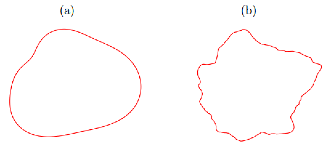
Figure 2: Star-shaped objects with radius defined by (a) a trigonometric polynomial (11) with $Q=5$ and (b) a piecewise approximation (14) built from a uniform mesh $(\theta_{j},r_{j})$, $j=0,\ldots,Z$, $Z=500$, with step $1/Z$.

To quantify uncertainty in the solution of the inverse problem, we resort to Bayes’ formula [28, 48] in finite dimension:

$$p_{\rm pt}(\boldsymbol{\nu}):=p(\boldsymbol{\nu}|\mathbf{d})={p(\mathbf{d}|\boldsymbol{\nu})\over p(\mathbf{d})}p_{\rm pr}(\boldsymbol{\nu}).$$ (15)

Here, the prior density of the variables $p_{\rm pr}(\cdot)$ incorporates available expert knowledge, while $p(\mathbf{d}|\boldsymbol{\nu})$ represents the conditional probability (or likelihood) of the observations $\mathbf{d}$ given the variables $\boldsymbol{\nu}$. The solution of the Bayesian inverse problem is the posterior density $p_{\rm pt}(\boldsymbol{\nu}|\mathbf{d})$ of the parameters given the data. The density $p(\mathbf{d})$ is a normalization factor that does not depend on the parameters. We choose a likelihood $p(\mathbf{d}|\boldsymbol{\nu})$

$$p(\mathbf{d}|\boldsymbol{\nu})={1\over(2\pi)^{N/2}\sqrt{|\boldsymbol{\Gamma}_{\!\rm{n}}|}}\exp\Big{(}-{1\over 2}\|\mathbf{f}(\boldsymbol{\nu})-\mathbf{d}\|^{2}_{\boldsymbol{\Gamma}_{\!\rm{n}}^{-1}}\Big{)}.$$ (16)

Here, $\|\mathbf{v}\|_{\boldsymbol{\Gamma}_{\!\rm{n}}^{-1}}^{2}=\mathbf{\overline{v}}^{t}\boldsymbol{\Gamma}_{\!\rm{n}}^{-1}\mathbf{v}$ and $\mathbf{f}(\boldsymbol{\nu})$ represents the measurement operator associated to parameters $\boldsymbol{\nu}$, that is,

$$\mathbf{f}(\boldsymbol{\nu})=\left(U_{\Omega_{\boldsymbol{\nu}},\mu_{\rm i}}(\mathbf{r}_{k},0,t_{m})\right)_{k=1,\ldots,K,m=1,\ldots,M},$$ (17)

where $U_{\Omega_{\boldsymbol{\nu}},\mu_{\rm i}}$ is the solution of the forward problem and $N=KM$.

We typically choose $p_{\rm pr}(\boldsymbol{\nu})$ as a multivariate Gaussian or a log Gaussian, see Section 4.2 for details. We could implement this approach using prior information obtained by any means, for instance, other imaging systems or other imaging algorithms, see [45]. In the absence of this information, the next section explains how to generate prior knowledge from the data.

4 Topological priors for the anomalies

Topological energy methods provide prior information on the number, location and size of the anomalies by splitting the recorded data in two halfs: dodd represents the data mesured at times $t_{2m+1}$ and deven the data measured at times $t_{2m}$: We exploit deven to generate prior information on the anomalies using the topological energy of the deterministic cost functional (8). The remaining half of the data dodd enters the likelihood (16), as we will explain later.

4.1 Calculation of topological energies

Given data $\mathbf{d}_{\rm even}$, the topological energy [13, 14] for the cost

$$J(\Omega)={1\over 2}\int_{\Gamma_{obs}}\int_{0}^{\tau_{\rm end}}|u_{\Omega}(\mathbf{x},s)-\mathbf{d}_{\rm even}(\mathbf{x},s)|^{2}dsdx,$$ (18)

$u_{\Omega}$ being the solution of (3)-(6) is given by

$$E(\mathbf{x})=\int_{0}^{\tau_{\rm end}}|U(\mathbf{x},s)|^{2}|P(\mathbf{x},s)|^{2}ds,$$ (19)

where $U=u_{\Omega}$ and $P$ is the associated adjoint field that appears in the calculation of topological derivatives [34]. In our set-up, we consider the observation set $\Gamma_{\rm obs}$ to be a set of receivers. Thus, $\int_{\Gamma_{\rm obs}}$ in (18) becomes a sum of values at the receivers $\mathbf{r}_{k}$. Since we record data at discrete time values $t_{2m}$, we approximate $\int_{0}^{\tau_{\rm end}}$ by a sum of values at such times too. Setting $\Omega=\emptyset$, the forward $U$ and adjoint $P$ fields are given by

$$\begin{array}[]{ll}U_{tt}-c^{2}\Delta U=f(t)g(\mathbf{x}),&\mathbf{x}\in R,\\[4.30554pt] {\partial U\over\partial\mathbf{n}}=0,&\mathbf{x}\in\partial R,\\[4.30554pt] U(\mathbf{x},0)=0,U_{t}(\mathbf{x},0)=0,&\mathbf{x}\in R,\end{array}$$ (23)

for $t\in[0,\tau_{\rm end}]$ and

$$\begin{array}[]{ll}[P_{tt}-c^{2}\Delta P](\tau_{\rm end}\!-\!t)=-(U\!-\!\mathbf{d}_{\rm even})(\tau_{\rm end}\!-\!t)\sum_{k=1}^{K}\delta_{\mathbf{r}_{k}},&\mathbf{x}\in R,\\[4.30554pt] {\partial P\over\partial\mathbf{n}}=0,&\mathbf{x}\in\partial R,\\[4.30554pt] P(\mathbf{x},\tau_{\rm end})=0,P_{t}(\mathbf{x},\tau_{\rm end})=0,&\mathbf{x}\in R,\end{array}$$ (27)

for $t\in[\tau_{\rm end},0]$. Here, $c$ is a constant equal to the healthy tissue wavespeed everywhere and $\delta_{\mathbf{r}_{k}}$ represent Dirac masses supported at the receivers. For computational purposes, we replace them by Gaussian regularizations. Notice that problems (23) and (27) can be solved computationally even when $c_{\rm i}$ and $\mu_{\rm i}$ are unknown. This is an advantage over alternative methods based on topological derivatives [34] which require the knowledge of these parameters. The fact that spurious oscillations in the presence of multiple objects are considerably reduced constitutes an additional asset. Topological energies are somewhat related to backpropagation techniques [49] and have been exploited for nondestructive testing of materials and tissues in [13, 14, 44].

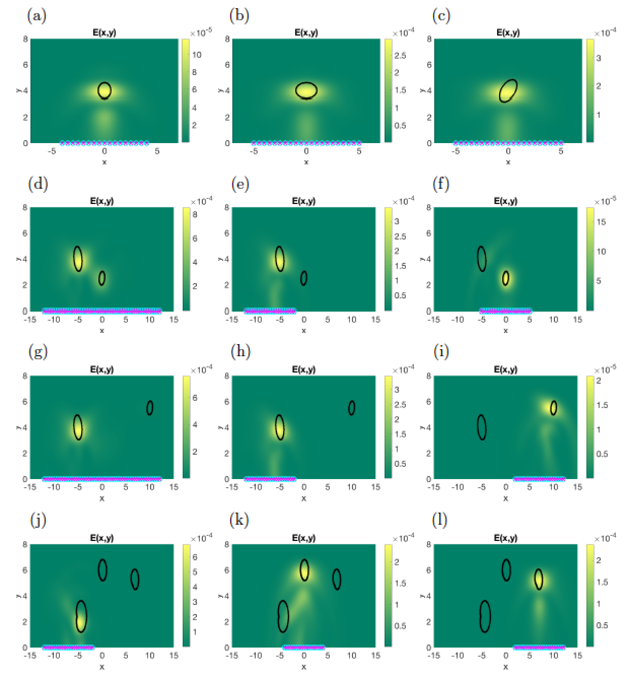
Figure 3: Topological energy fields for: single objects with different sizes and orientations (a) circle, (b) ellipse, (c) rotated ellipse; two objects under different emitter/receiver configurations (d),(g) centered, (e),(h) left sided, (f),(i) right sided; and three star-shaped objects (j)-(l) sweeping the bottom region. Crosses and circles represent emitters and receivers, located at the same position. Black curves represent the true objects. Noise level in the data: $10$ %.

The previous description assumes that we record data at the receivers from the time $t=0$ at which we start to emit. If we start the recording later, at a time $\tau_{\rm in}$, formula (18) integrates from $\tau_{\rm in}$ to $\tau_{\rm end}$ and the right hand side in (27) is only non zero in $[\tau_{\rm in},\tau_{\rm end}]$. We set the final time $\tau_{\rm end}\sim 2{H\over c}$, where $H$ is the expected resolution depth.

Figure 3 shows the topological energy fields obtained for several object geometries under different emitter/receiver configurations for the parameter values specified in A.2, after removing dimensions. The data $\mathbf{d}_{\rm even}$ used to calculate them are synthetic: they are generated by solving numerically the nondimensionalized forward problem (47) in the presence of the true objects, evaluating the solution in the selected space/time datagrid and adding $10$% noise, as explained in Section 2. To prevent inverse crimes, the fields $U$ in (23) and $P$ in (27) are approximated numerically using rougher meshes: the spatial and time steps for them are twice the steps used when solving numerically to generate the data, and the spatial meshes vary. We have set $\tau_{\rm in}=2$ (value at which $f(t)$ almost vanishes for our parameter choice) and $H=7$ in the calculation of the topological energy.

4.2 Prior construction

Once the topological fields are calculated, we construct a first guess $\Omega_{0}$ for the anomalies immersed in a background medium $R$ by exploiting the peaks of the topological energy:

$$\Omega_{0}=\left\{\mathbf{x}\in R\;|\;E(\mathbf{x})>(1-C_{0})\,{\rm max}_{\mathbf{y}\in R}E(\mathbf{y})\right\},$$ (28)

where $C_{0}\in(0,1)$ is such that $J(\Omega_{0})<J(\emptyset).$ In case several objects are present, we obtain more precise information by sequentially activating fractions of the whole network of emitters/receivers, as shown in Figure 3(d)-(l). We fit circles to the dominant peaks found for each fraction. In this way, we are able to detect all the anomalies. Instead, when we use the information coming from the whole network, we often find the most prominent anomaly only. We use this information to construct priors for the two types of star-shaped parameterizations we consider as follows.

Assuming we locate $L$ peaks, we fit to them circles parametrized by $\boldsymbol{\nu}_{0}=(\boldsymbol{\nu}^{1}_{0},\ldots,\boldsymbol{\nu}^{L}_{0})$. When we work with the representation (9)-(11), we set

$$\boldsymbol{\nu}^{\ell}_{0}=(c_{x,0}^{\ell},c_{y,0}^{\ell},a_{0,0}^{\ell},b_{1,0}^{\ell},a_{1,0}^{\ell},\ldots,b_{Q,0}^{\ell},a_{Q,0}^{\ell},\mu_{\rm i,0}^{\ell}),\quad\ell=1,\ldots,L,$$ (29)

where $c_{x,0}^{\ell},c_{y,0}^{\ell}$ is the center of mass of each component, $a_{0,0}^{\ell}$ half the smallest diameter, and $a_{1,0}^{\ell}=\ldots=a_{Q,0}^{\ell}=b_{1,0}^{\ell}=\ldots=b_{Q,0}^{\ell}=0$. We also set $\mu_{\rm i,0}^{\ell}=\mu$, the known background value for the healthy tissue. Then, we choose $p_{\rm pr}(\boldsymbol{\nu})$ as a multivariate Gaussian with covariance matrix $\boldsymbol{\Gamma}_{\!\rm{pr}}$

$$\begin{array}[]{l}p_{\rm pr}(\boldsymbol{\nu})={1\over(2\pi)^{n/2}}{1\over\sqrt{|\boldsymbol{\Gamma}_{\!\rm{pr}}|}}\exp(-{1\over 2}(\boldsymbol{\nu}-\boldsymbol{\nu}_{0})^{t}\boldsymbol{\Gamma}_{\!\rm{pr}}^{-1}(\boldsymbol{\nu}-\boldsymbol{\nu}_{0})),\end{array}$$ (31)

where $n$ is the dimension of $\boldsymbol{\nu}_{0}$, provided that $\mu_{\rm i}^{\ell}>0$, the curves associated to the parameterization $\boldsymbol{\nu}$ fulfill $r^{\ell}(\theta)>0$, for $\theta\in[0,1]$ and all $\ell$, they do not intersect, and they do not form nested configurations. Otherwise, $p_{\rm pr}(\boldsymbol{\nu})$ is set equal to zero. Notice that $r^{\ell}(\theta)>0$ is not a condition on the sign of the curve parameters, but on the sign of the combination (11). We choose a diagonal covariance matrix $\boldsymbol{\Gamma}_{\!\rm{pr}}$ formed by $L$ blocks. In our numerical tests, each block starts with $(\sigma_{x}^{\ell})^{2}=(\sigma_{y}^{\ell})^{2}=0.1$ and ends with $(\sigma_{\mu})^{2}=20^{2}.$ Then $(\sigma_{a_{0}}^{\ell})^{2}=0.1$ and $(\sigma_{a_{q}}^{\ell})^{2}=(\sigma_{b_{q}}^{\ell})^{2}=0.1/(1+q^{2})^{s}$, $1\leq q\leq Q$, $s$ large, as in [9], so that the prior favors regular shapes with $r(t)>0$. Typically, we fix $s=3$ and $Q=5$.

When we work with the representation (12)-(14), we set

$$\boldsymbol{\nu}^{\ell}_{0}=(c_{x,0}^{\ell},c_{y,0}^{\ell},r_{0,0}^{\ell},r_{1,0}^{\ell},\ldots,r_{Z-1,0}^{\ell},\mu_{\rm i,0}^{\ell}),\quad\ell=1,\ldots,L,$$ (32)

where $c_{x,0}^{\ell},c_{y,0}^{\ell}$ is the center of mass of each component, $r_{0,0}^{\ell}=r_{1,0}^{\ell}=\ldots=r_{Z-1,0}^{\ell}$ is half the smallest diameter and $\mu_{\rm i,0}^{\ell}=\mu$. Notice that $r_{Z,0}=r_{0,0}$. We choose $p_{\rm pr}(\boldsymbol{\nu})$ as the product of multivariate Gaussians for the variables $c_{x,0}^{\ell}$, $c_{y,0}^{\ell}$, $\mu_{\rm i,0}^{\ell}$, with the same standard deviations as before, and log Gaussian distributions for $r_{0,0}^{\ell},r_{1,0}^{\ell},\ldots,r_{Z-1,0}^{\ell},$ with Matern covariance matrices, see [15]. We use for the Matern covariance between points $(\cos(\theta_{i}),\sin(\theta_{i}))$ and $(\cos(\theta_{j}),\sin(\theta_{j}))$ separated by a distance $d$ the expressions [43]

$$C_{\nu,\rho,\sigma}(d)=\sigma^{2}{2^{1-\nu}\over\Gamma(\boldsymbol{\nu})}\left(\sqrt{2\nu}{d\over\rho}\right)^{\nu}K_{\nu}\left(\sqrt{2\nu}{d\over\rho}\right),$$

where $\Gamma$ is the Gamma function, $K_{\nu}$ the modified Bessel function of the second kind, and $\nu$, $\rho$, $\sigma$ are parameters. In our numerical tests we fix $\nu=3/2$, $\sigma=0.2$, $\rho=0.5$.

5 Markov Chain Monte Carlo sampling

We insert the prior distributions obtained in the previous section in the posterior probability $p_{\rm pt}$ given by (15) and (16), with the data $\mathbf{d}_{\rm odd}$ not used to produce the prior information. Then we can sample the unnormalized posterior distribution $q(\boldsymbol{\nu})=p(\mathbf{d}_{\rm odd}|\boldsymbol{\nu})p_{\rm pr}(\boldsymbol{\nu})$ using Markov Chain Monte Carlo (MCMC) methods. Note that the unknown scaling factor $p(\mathbf{d})$ in (15) is not needed for MCMC sampling. Standard MCMC methods, such as Metropolis-Hastings or Hamiltonian MonteCarlo [37], produce a chain of $N$-dimensional states $\boldsymbol{\nu}^{(0)}\longrightarrow\boldsymbol{\nu}^{(1)}\ldots\longrightarrow\boldsymbol{\nu}^{(i)}\ldots$ which evolve to be distributed according to the target distribution. One first samples an initial state $\boldsymbol{\nu}^{(0)}$ from the prior distribution, and then moves from one state $\boldsymbol{\nu}^{(i)}$ to the next $\boldsymbol{\nu}^{(i+1)}$ guided by a transition operator. More recent ensemble MCMC samplers [16, 23] draw $W$ initial states (the ‘walkers’ or ‘particles’) from the prior distribution and transition to new states while mixing them to construct the chain. This allows us to handle multimodal posteriors [9] and to parallelize the process for faster exploration of the structure of the posterior distribution.

Different ensemble samplers adapt better to the different parametrizations we consider for the anomalies. Affine-invariant samplers perform well in our set-up. We have considered two. The first one is a stretch move based Affine Invariant Ensemble Sampler (SAIES), see [23]:

• Initialization: Choose $W$ initial states $\boldsymbol{\nu}_{w}^{(1)}\in\mathbb{R}^{d}$, $w=1,\ldots,W,$ with probability $\pi$ (the prior probability $p_{\rm pr}$ in our case) and a value $a>1$.

• For each step $s=1,\ldots,S$,

  • For each $w=1,\ldots,W$

    • Draw $\boldsymbol{\nu}_{q}^{(s)}$ at random from the set $\{\boldsymbol{\nu}_{j}^{(s)}\}_{j\neq w}$.

    • Choose a random value $z_{w}$ from the distribution $g(z)={1\over\sqrt{z}}$ when $z\in[1/a,a]$, zero otherwise.

    • Set $\boldsymbol{\nu}_{w,\rm prop}^{(s)}=\boldsymbol{\nu}_{w}^{(s)}+z_{w}(\boldsymbol{\nu}_{w}^{(s)}-\boldsymbol{\nu}_{q}^{(s)}).$

    • Set $\boldsymbol{\nu}_{w}^{(s+1)}=\boldsymbol{\nu}_{w,\rm prop}^{(s)}$ with probability ${\rm min}\left\{1,z_{w}^{d-1}{p_{\rm pt}(\boldsymbol{\nu}_{w,\rm prop}^{(s)})\over p_{\rm pt}(\boldsymbol{\nu}_{w}^{(s)})}\right\},$ or else keep $\boldsymbol{\nu}_{w}^{(s+1)}=\boldsymbol{\nu}_{w}^{(s)}.$

• Output: The samples $\boldsymbol{\nu}_{w}^{(s)}$, $w=1,\ldots,W$, $s=1,\ldots,S$.

The second one is a general Affine Invariant Ensemble Sampler (AIES), which proceeds as follows, see [16] for instance:

• Initialization: Choose $W$ initial states $\boldsymbol{\nu}_{w}^{(1)}\in\mathbb{R}^{d}$, $w=1,\ldots,W$, with probability $\pi$ (the prior probability $p_{\rm pr}$ in our case) and a value $\lambda>0$.

• For each step $s=1,\ldots,S$,

  • For each $w=1,\ldots,W$

    • Set $\overline{\boldsymbol{\nu}}={1\over W-1}\sum_{j\neq w}\boldsymbol{\nu}_{j}^{(s)}$.

    • Draw $z_{w}$ with probability ${\cal N}(0,1).$

    • Set $\boldsymbol{\nu}_{w,\rm prop}^{(s)}=\boldsymbol{\nu}_{w}^{(s)}+{\lambda\over\sqrt{W-1}}\sum_{j\neq w}z_{j}(\boldsymbol{\nu}_{j}^{(s)}-\overline{\boldsymbol{\nu}}).$

    • Set $\boldsymbol{\nu}_{w}^{(s+1)}=\boldsymbol{\nu}_{w,\rm prop}^{(s)}$ with probability ${\rm min}\left\{1,{p_{\rm pt}(\boldsymbol{\nu}_{w,\rm prop}^{(s)})\over p_{\rm pt}(\boldsymbol{\nu}_{w}^{(s)})}\right\},$ or else keep $\boldsymbol{\nu}_{w}^{(s+1)}=\boldsymbol{\nu}_{w}^{(s)}.$

• Output: The samples $\boldsymbol{\nu}_{w}^{(s)}$, $w=1,\ldots,W$, $s=1,\ldots,S$.

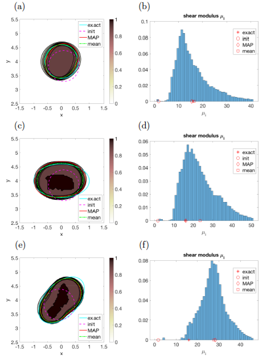
Figure 4: (a), (c), (e) True objects versus MAP estimate and sample mean calculated from MCMC samples for different geometries. The contour levels represent the probability of belonging to the object. (b), (d), (f) Histograms quantifying uncertainty of the MAP estimate and mean values for $\mu_{\rm i}$. Parameters and samplers: SAIES with $a=2$, $\tilde{S}=500$, $W=480$ and $B=W\tilde{S}/5$.

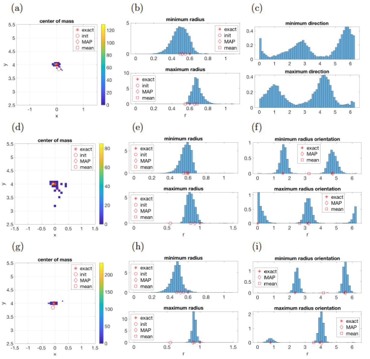
Figure 5: Histograms representing a discrete approximations of the densities for the distribution of the centers of mass (a), (d), (g), radius size (b), (e), (h), and orientation (c), (f), (i) in the three test geometries considered in Figure 4. Same sampling parameters.

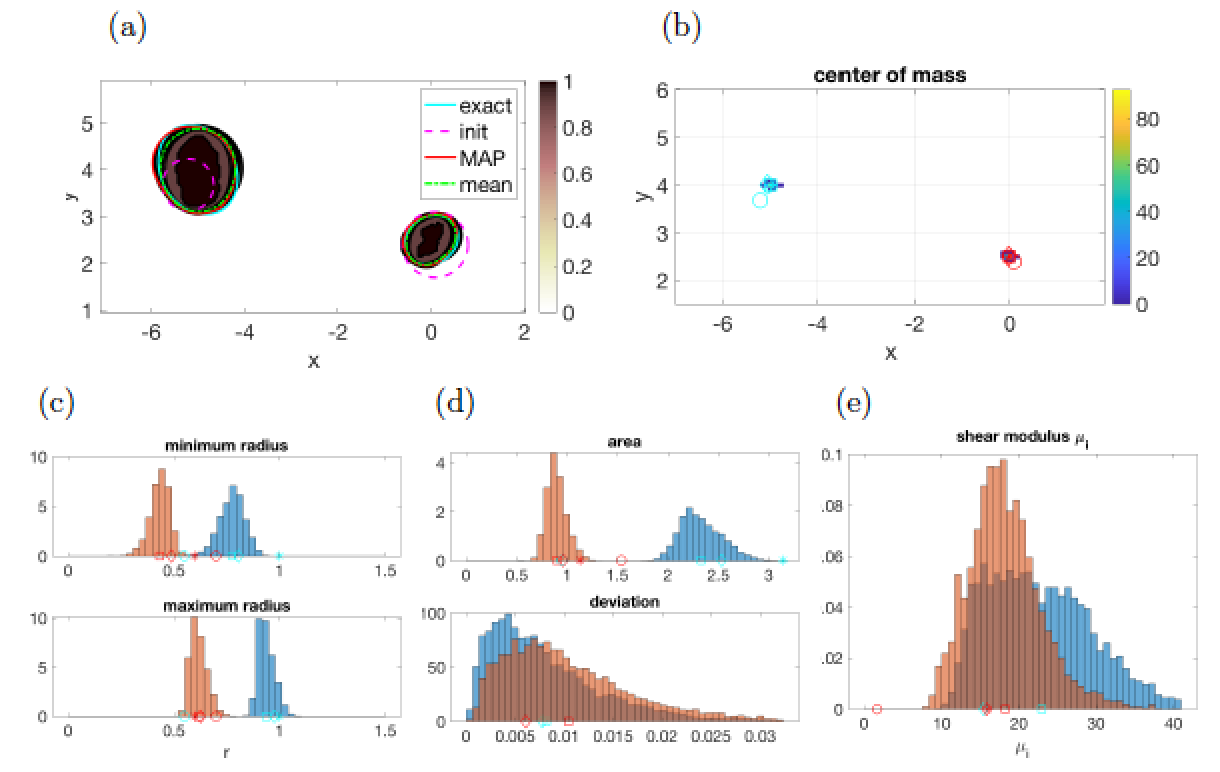
Figure 6: (a) True objects versus MAP estimate and mean calculated from MCMC samples. The contour levels represent the probability of belonging to the object. Superimposed curves represent the exact contours (solid light cyan), the MAP point (solid dark red), the mean (dash-dotted green), and the initial guess (dashed magenta). (b) Histograms representing discrete approximations of the densities for the distribution of the centers of mass. (c)-(d) Histograms for the radius sizes (c), area and deviation from a circular object (d) and shear modulus $\mu_{\rm i}$ (e). Blue histograms and cyan symbols correspond to the large object, orange histograms and red symbols to the small one (asterisk: exact value, circle: initial value, diamond: MAP point, square: mean). Parameters and samplers: SAIES with $a=2$, $\tilde{S}=500$, $W=480$ and $B=W\tilde{S}/5$.

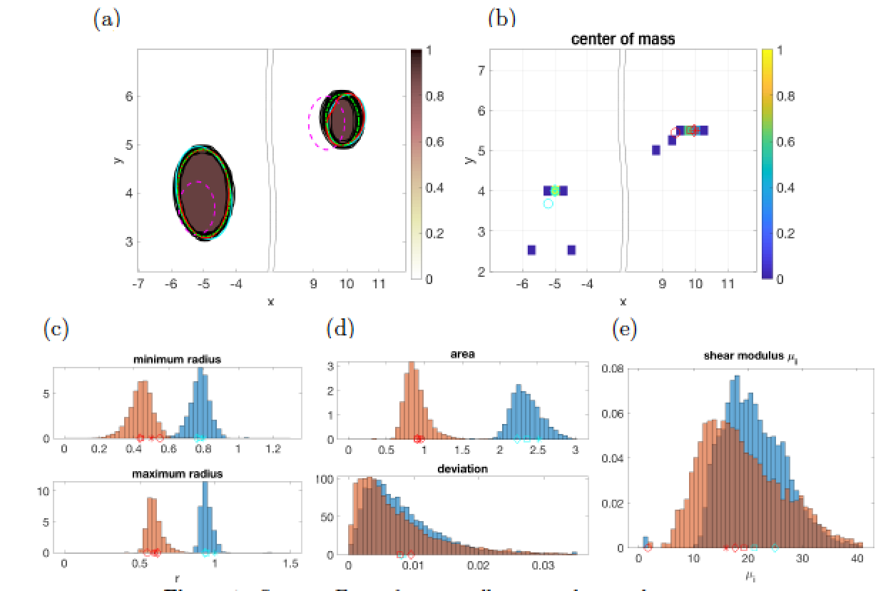
Figure 7: Same as Fig. 6 for two well separated anomalies.

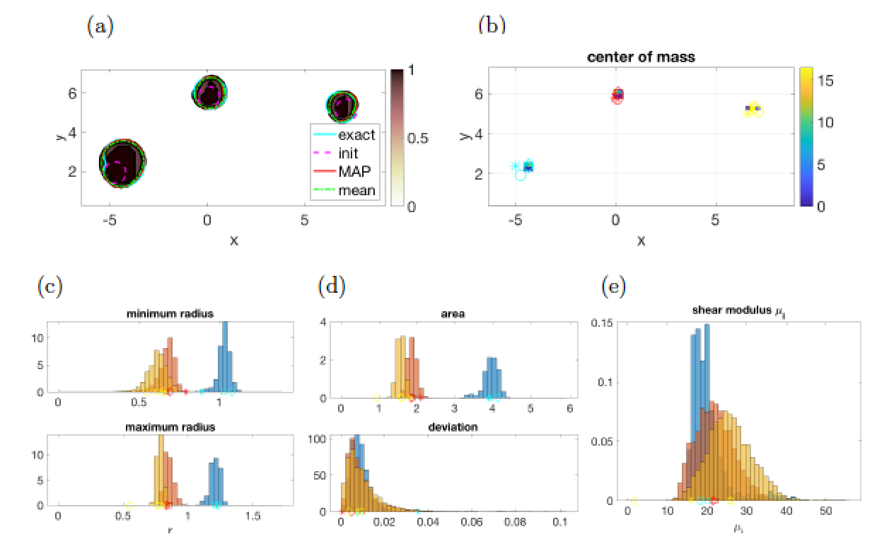
Figure 8: Same as Figure 6 for a configuration with three objects. Orange histograms and red symbols correspond to the middle object, blue histograms and cyan symbols to the left-most one, yellow histograms and symbols to the right-most one.

While the first sampler evolves faster in low dimensions $d$, it usually requires $W>2d$ to perform properly. In principle, the general AIES can be more robust as dimension grows. Figures 4-8 display results with SAIES for smooth shapes admitting low dimensional parametrizations. AIES provides similar results doubling the number of steps. Section 7 considers high dimensional irregular shapes. There, AIES perfoms reasonably well with $W$ slightly larger than $d$. In both cases and for each $w$, we keep one of each three samples up to a total number of $\tilde{S}=S/3$ to reduce correlations and discard the first $\tilde{S}/5$ as a burn in period. We have set $\sigma_{\rm noise}=\alpha\,{\rm max}|d^{k}_{n,{\rm true}}|/100$ in $\boldsymbol{\Gamma}_{\!\rm{n}}$ with $\alpha=10$.

Here, for highly smooth shapes, we consider the parameter set (29) and define $\boldsymbol{\Gamma}_{\!\rm{pr}}$ as in Section 4.2. Then, we insert the prior probability (31) obtained by topological methods and the likelihood (16) in the posterior probability (15) to be sampled. From the samples, we obtain information on the most likely values for $\boldsymbol{\nu}$, that is, the maximum a posteriori (MAP) estimate and the uncertainty about it, depicted in figures 4-8. Figure 4 illustrates the uncertainty in the shape of the anomaly and the value of the parameter representing the dimensionless shear modulus $\mu_{\rm i}$ for single shapes: a circle and an ellipse with different orientations. The sample with highest probability defines the MAP point and the mean of the parameters corresponding to all the samples defines a mean estimate. The location and shape of the anomalies is reasonably well captured by both, see also Figure 5 for the uncertainty in geometrical features of interest, such as the location of the center of mass, the size of the largest and smallest diameters and their orientation. However, the value of the shear modulus displays larger uncertainty, still in the range indicating sickness. The histograms reveal distributions with wide and asymmetric tails. Notice that a change in the orientation of an object can drastically increase uncertainty in the predictions, compare Fig. 4(d) and Fig. 4(f).

Figures 6-8 consider configurations with multiple anomalies. The approximation of the shapes provided by the MAP point and the mean values in figures 6-8 is quite reasonable, regarding both the shapes, their basic geometrical features and the shear modulus, though we observe again wide asymmetric tails.

When we include in the prior less anomalies than needed, the distribution may be multimodal: we may spot the missing components. When we include in the prior more anomalies than needed, the spurious ones may essentially vanish because $\mu_{\rm i}$ is basically equal to $\mu$. Notice that our priors contained the correct number of anomalies. The resulting distributions represent a single mode. Also, the means and the MAP points are reasonably close. This suggests that optimization schemes could capture the MAP estimate, allowing for a Laplace approximation of the posterior distribution, which can be sampled at a much lower cost. The computational time drops from a few days to a few minutes.

6 Sampling from a Bayesian linearized formulation

To reduce the computational cost, we analyze the Laplace approximation of the posterior density (15) obtained by linearization at the maximum a posteriori (MAP) point $\boldsymbol{\nu}_{\!\rm{\scriptscriptstyle MAP}}$. This strategy first computes the vector $\boldsymbol{\nu}_{\!\rm{\scriptscriptstyle MAP}}$, which minimizes the negative log likelihood

$$J(\boldsymbol{\nu})={1\over 2\sigma_{\rm noise}^{2}}\sum_{m=1}^{M}\sum_{k=1}^{K}|U_{\boldsymbol{\nu}}(r_{k},0,t_{m})\!-\!d_{k}^{m}|^{2}+{1\over 2}(\boldsymbol{\nu}-\boldsymbol{\nu}_{0})^{t}\boldsymbol{\Gamma}_{\!\rm{pr}}^{-1}(\boldsymbol{\nu}-\boldsymbol{\nu}_{0}),$$ (33)

where $U_{\boldsymbol{\nu}}$ is the solution of the forward problem with object $\Omega$ parametrized by $\boldsymbol{\nu}$ given by (9). Then, we approximate the posterior distribution by a multivariate Gaussian ${\cal N}(\boldsymbol{\nu}_{\!\rm{\scriptscriptstyle MAP}},\boldsymbol{\Gamma}_{\!\rm{pt}})$ with posterior convariance matrix $\boldsymbol{\Gamma}_{\!\rm{pt}}=\mathbf{H}_{\boldsymbol{\nu}_{\!\rm{\scriptscriptstyle MAP}}}^{-1}$, where $\mathbf{H}_{\boldsymbol{\nu}_{\!\rm{\scriptscriptstyle MAP}}}$ is an approximation of the Hessian of the measurement operator (17) evaluated at $\boldsymbol{\nu}_{\!\rm{\scriptscriptstyle MAP}}$ [5, 51].

6.1 Computing the MAP point

The MAP point is calculated exploiting techniques of deterministic optimization. Taking the prior $\boldsymbol{\nu}_{0}$ as initial guess of the parametrization, that is, $\boldsymbol{\nu}^{0}=\boldsymbol{\nu}_{0}$, we can implement the Newton type iteration $\boldsymbol{\nu}^{j+1}=\boldsymbol{\nu}^{j}+\boldsymbol{\xi}^{j+1}$ where $\boldsymbol{\xi}^{j+1}$ is the solution of

$$\left(\mathbf{H}(\boldsymbol{\nu}^{j})+\omega_{j}{\rm diag}(\mathbf{H}(\boldsymbol{\nu}^{j}))\right)\boldsymbol{\xi}^{j+1}=-\mathbf{g}(\boldsymbol{\nu}^{j}),$$ (34)

see [19], where $\mathbf{H}(\boldsymbol{\nu})$ and $\mathbf{g}(\boldsymbol{\nu})$ represent the Hessian and the gradient of the cost. In practice, to reduce the occurrence of negative radii and the risk of loop formation in the curves, we introduce an additional parameter $\lambda>0$, replacing (33) by

$$J_{\lambda}(\boldsymbol{\nu})={1\over 2\sigma_{\rm noise}^{2}}\sum_{m=1}^{M}\sum_{k=1}^{K}|U_{\boldsymbol{\nu}}(r_{k},0,t_{m})\!-\!d_{k}^{m}|^{2}\!+\!{\lambda\over 2}(\boldsymbol{\nu}-\boldsymbol{\nu}_{0})^{t}\boldsymbol{\Gamma}_{\!\rm{pr}}^{-1}(\boldsymbol{\nu}-\boldsymbol{\nu}_{0})$$ (35)

and (34) by

$$\left(\mathbf{H}^{\rm GN}_{\lambda_{j}}(\boldsymbol{\nu}^{j})+\omega_{j}{\rm diag}(\mathbf{H}^{\rm GN}_{\lambda_{j}}(\boldsymbol{\nu}^{j}))\right)\boldsymbol{\xi}^{j+1}=-\mathbf{g}_{\lambda_{j}}(\boldsymbol{\nu}^{j}).$$ (36)

Here, the subscript $\lambda_{j}$ indicates that we multiply $\boldsymbol{\Gamma}_{\!\rm{pr}}^{-1}$ by a factor $\lambda_{j}$ in the initial iterations to balance the two terms defining the cost $J$ in (33). Notice that we have also replaced the full Hessian by the Gauss-Newton part of the Hessian to reduce the computational cost per iteration. The components of $\mathbf{H}^{\rm GN}_{\lambda}(\boldsymbol{\nu})$ and $\mathbf{g}_{\lambda}(\boldsymbol{\nu})$ are given by:

$$(g_{\lambda}(\boldsymbol{\nu}))_{i} ={\partial J(\boldsymbol{\nu})\over\partial\nu_{i}} ={1\over\sigma^{2}_{\rm noise}}\sum_{m=1}^{M}\sum_{k=1}^{K}(U_{\boldsymbol{\nu}}(r_{k},0,t_{m})-d_{k}^{m}){\partial U_{\boldsymbol{\nu}}\over\partial\nu_{i}}(r_{k},0,t_{m})$$ (37)

$$+\lambda[\boldsymbol{\Gamma}_{\!\rm{pr}}^{-1}(\boldsymbol{\nu}-\boldsymbol{\nu}_{0})]_{i},$$

$$(\mathbf{H}^{\rm GN}_{\lambda}(\boldsymbol{\nu}))_{i,\ell} ={\partial^{2}J(\boldsymbol{\nu})\over\partial\nu_{i}\partial\nu_{\ell}} \sim{1\over\sigma^{2}_{\rm noise}}\sum_{m=1}^{M}\sum_{k=1}^{K}{\partial U_{\boldsymbol{\nu}}\over\partial\nu_{i}}(r_{k},0,t_{m}){\partial U_{\boldsymbol{\nu}}\over\partial\nu_{\ell}}(r_{k},0,t_{m})$$ (38)

$$+\lambda[\boldsymbol{\Gamma}_{\!\rm{pr}}^{-1}]_{i,\ell}.$$

The second order derivatives of $U_{\boldsymbol{\nu}}$ are neglected.

To optimize our objective function we implement a double iteration:

• Initially, we set $\omega_{0}=10^{-4}/2$, $\lambda_{0}=0.1\sigma_{\rm noise}^{-2}$, and $\boldsymbol{\nu}^{0}=\boldsymbol{\nu}_{0}$.

• At each step we calculate $\boldsymbol{\nu}^{j+1}=\boldsymbol{\nu}^{j}+\boldsymbol{\xi}^{j+1}$, where $\boldsymbol{\xi}^{j+1}$ is the solution of (36). Then

  • We check i) if $r(\theta)>0$, $r(\theta)$ given by (11), and if $\mu_{\rm i}>0.5\mu$, ii) if the functional $J_{\lambda_{j}}(\boldsymbol{\nu})$ decreases replacing $\boldsymbol{\nu}^{j}$ with $\boldsymbol{\nu}^{j+1}$.

  • If any of these conditions fails, we do not accept $\boldsymbol{\xi}^{j+1}$. We increase $\omega_{j}$ by a factor $2$, solve again (36) and check conditions i) and ii) until they are fulfilled.

  • If both conditions are satisfied, we accept $\boldsymbol{\xi}^{j+1}$ and set $\omega_{j+1}=\omega_{j}/2$ and $\lambda_{j+1}={\rm max}(\lambda_{j}/5,1)$.

• After a few steps $j_{0}$, $\lambda_{j+1}=1$ for $j\geq j_{0}$. When the relative difference between the new value of the cost and the previous one is smaller than a tolerance Tol (here Tol $=5\times 10^{-7}$), we freeze all the components except $\mu_{\rm i}^{j+1}$ and iterate with respect to $\mu_{\rm i}$ until variations fall below a threshold $0.02$.

To evaluate the derivatives ${\partial U_{\boldsymbol{\nu}}\over\partial\nu_{i}}(r_{k},0,t_{m})$ required for the calculation of (37)-(38) at each step, we use the approximation

$${\partial U_{\boldsymbol{\nu}}\over\partial\nu_{i}}(r_{k},0,t_{m})\sim{U_{\boldsymbol{\nu}+\eta_{i}}(r_{k},0,t_{m})-U_{\boldsymbol{\nu}}(r_{k},0,t_{m})\over\eta_{i}}$$

with $\eta_{i}$ small, $U_{\boldsymbol{\nu}+\eta_{i}}$ being the solution of the forward problem with $\nu_{i}$ replaced by $\nu_{i}+\eta_{i}.$ All the forward problems are solved with the same discretization and steps we used in Section 5. The values of $\eta_{i}$ must be calibrated. Initially, we set for each block $\ell=1,\ldots,L$ in (9) $\eta_{1}^{\ell}=\eta_{2}^{\ell}=\eta_{3}^{\ell}=\eta_{2Q+4}^{\ell}=\eta=0.1$ and $\eta_{3+2i}^{\ell}=\eta_{2+2i}^{\ell}=\eta/2$ for $i=1,\ldots,Q$. As we iterate, we calibrate values for $\eta_{i}$ estimating the quotients ${D_{\nu_{i}}U_{\boldsymbol{\nu}^{j}}(r_{k},0,t_{m})\over D^{2}_{\nu_{i}}U_{\boldsymbol{\nu}^{j}}(r_{k},0,t_{m})}$, where $D$ and $D^{2}$ represent approximations of derivatives, and averaging over $k$ and $m$. In the tests we have performed, the choice

$$\eta_{1}^{\ell}=\eta_{2}^{\ell}=0.05,\quad\eta_{2Q+4}=0.15,$$

$$\eta_{3+2i}^{\ell}=\eta_{2+2i}^{\ell}=0.05,\quad i=1,\ldots,Q,$$

gives good results, with $\eta_{3}$ in the range $0.025-0.225$.

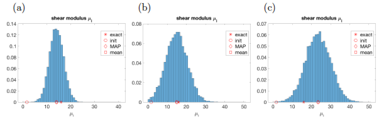
Figure 9: Counterpart of Fig. 4 (b), (d), (f) obtained by calculating the MAP point and linearizing the posterior probability about it. 10000 samples plotted.

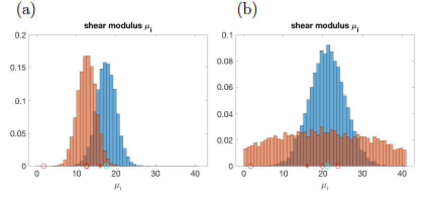
Figure 10: Counterparts of Fig. 6(b) and Fig. 7(b) obtained by linearized Bayesian methods. $10000$ samples plotted.

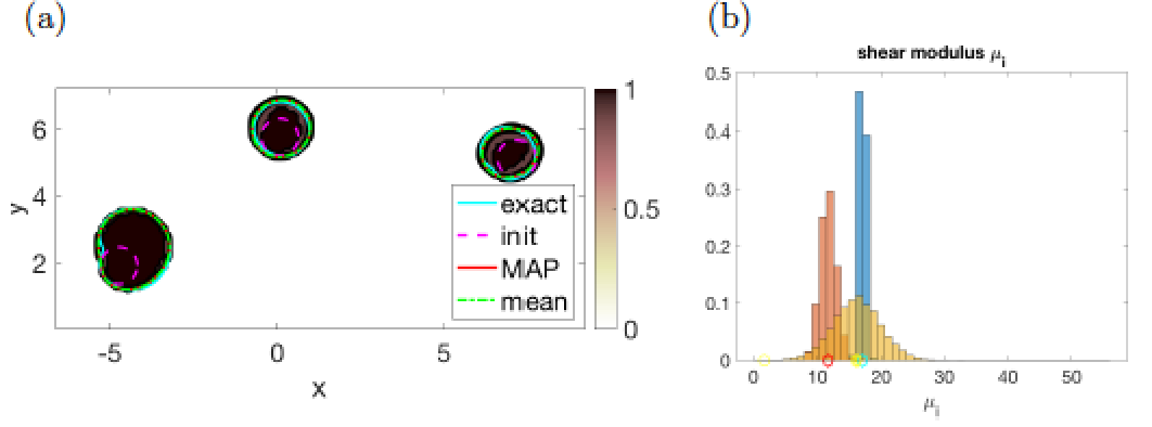
Figure 11: Counterpart of Fig. 8 obtained by linearized Bayesian methods. $10000$ samples plotted.

6.2 Sampling

Once we have obtained an approximation to $\boldsymbol{\nu}_{\!\rm{\scriptscriptstyle MAP}}$, we linearize the posterior distribution about it, approximate by a multivariate Gaussian distribution ${\cal N}(\boldsymbol{\nu}_{\!\rm{\scriptscriptstyle MAP}},\boldsymbol{\Gamma}_{\!\rm{pt}})$ and draw samples from it to quantify uncertainty. We set

$$\boldsymbol{\Gamma}_{\!\rm{pt}}=(\mathbf{F}(\boldsymbol{\nu}_{\!\rm{\scriptscriptstyle MAP}})^{t}\boldsymbol{\Gamma}_{\!\rm{n}}^{-1}\mathbf{F}(\boldsymbol{\nu}_{\!\rm{\scriptscriptstyle MAP}})+\boldsymbol{\Gamma}_{\!\rm{pr}}^{-1})^{-1}=\mathbf{H}^{\rm GN}(\boldsymbol{\nu}_{\!\rm{\scriptscriptstyle MAP}})^{-1},$$

where $\mathbf{F}(\boldsymbol{\nu}_{\!\rm{\scriptscriptstyle MAP}})=\left({\partial U_{\boldsymbol{\nu}_{\!\rm{\scriptscriptstyle MAP}}}\over\partial\nu_{i}}(p_{j})\right)_{j,i}$ and

$$\mathbf{p}=((r_{1},0,t_{1}),\ldots,(r_{K},0,t_{1}),\ldots,(r_{1},0,t_{M}),\ldots,(r_{K},0,t_{M})),$$

that is, $\mathbf{F}(\boldsymbol{\nu}_{\!\rm{\scriptscriptstyle MAP}})$ is the matrix with $i$th-column ${\partial U_{\boldsymbol{\nu}}\over\partial\nu_{i}}(r_{k},0,t_{m})$, $k=1,\ldots,K$, $m=1,\ldots,M$ evaluated at $\boldsymbol{\nu}_{\!\rm{\scriptscriptstyle MAP}}$. This can be done by means of the relation

$$\boldsymbol{\nu}=\boldsymbol{\nu}_{\rm MAP}+\boldsymbol{\Gamma}_{\!\rm{pt}}^{1/2}\mathbf{n},$$ (39)

$\mathbf{n}$ being a standard normal randomly generated vector (iid).

Figures 9-11 revisit the previous MCMC tests with this procedure. In each case, we optimize to approximate the MAP point and generate a large collection of samples of the posterior distribution by means of (39). The values of the cost for the approximated MAP estimates obtained this way are similar to those for the MAP estimates previously found by MCMC sampling. Comparing the results, we remark that the MAP points and contour curves for the shapes remain similar. Fig 11(a) illustrates this fact in the example with three objects. However, the values of $\mu_{\rm i}$ show larger variability. For single objects, the MAP points and mean values remain alike, while the wide asymmetric tails are lost. The tests with more objects show a similar tendency. Notice that as objects become smaller and distant, information can be lost, as it happens in the red histogram in Fig 10(b) (compare to Fig 7(b)).

The computational cost of this approach is much smaller. The MAP estimate for single objects is obtained in about $10$ steps, about $5$ minutes in a laptop using MATLAB, while MCMC sampling can take 2-4 days depending on the size of the computational regions.

7 Irregular shapes

Finally, we consider irregular shapes defined by high dimensional parametrizations of the form (12)-(14). We insert the prior distributions (32) obtained by topological methods in the posterior probability given by (15) and (16), with the data $\mathbf{d}_{\rm odd}$ not used to produce the prior information.

The affine-invariant ensemble sampler AIES described in Section 5 produces the results represented in Figure 12 for an irregular shape. Notice that the use of SAIES would require $W>2d=1006$ walkers, which would mix much more slowly. Now, the MAP estimate does not approach the true shape. Nevertheless, the mean profile and the contour plot give an idea of the location and size of the anomaly.

In the previous sections, the probability for negative $\mu_{\rm i}$ was set equal to zero. Now, $\mu_{\rm i}=\exp(\gamma)$, where $\gamma$ is the random variable that we sample. Notice the peak for $\mu_{\rm i}$ near zero. It is due to a family of large samples with small $\mu_{\rm i}$. Figure 12(c) represents the last $W$ samples we obtained. We observe a dominant family of samples which wrap around the true object. A second family is formed by smaller shapes with larger values of $\mu_{\rm i}$ placed between the object and the emitters, at the location of a small secondary peak of the topological energy (see Figure 3(c)). The third family corresponds to large samples with small $\mu_{\rm i}$ placed behind the true object. The sample distributions we obtain this way are multimodal, though the main mode dominates the rest when averaging to obtain a mean. Notice that uncertainty in the values of $\mu_{\rm i}$ with this procedure seems quite large. The prior information we use has low quality in this case. We look for an irregular shape assuming that the prior is a smooth circle and $\mu_{\rm i}$ is the value for the healthy tissue. Inconsistency between the prior and the data may lead to multimodality, as pointed out in the previous section.

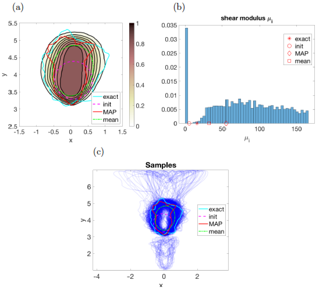
Figure 12: Results for the object in Figure 3(b) for $Z=500$. MCMC with AIES $W=600$, $\tilde{S}=3900$, $B=W\tilde{S}/2$ , $\lambda=0.2$.

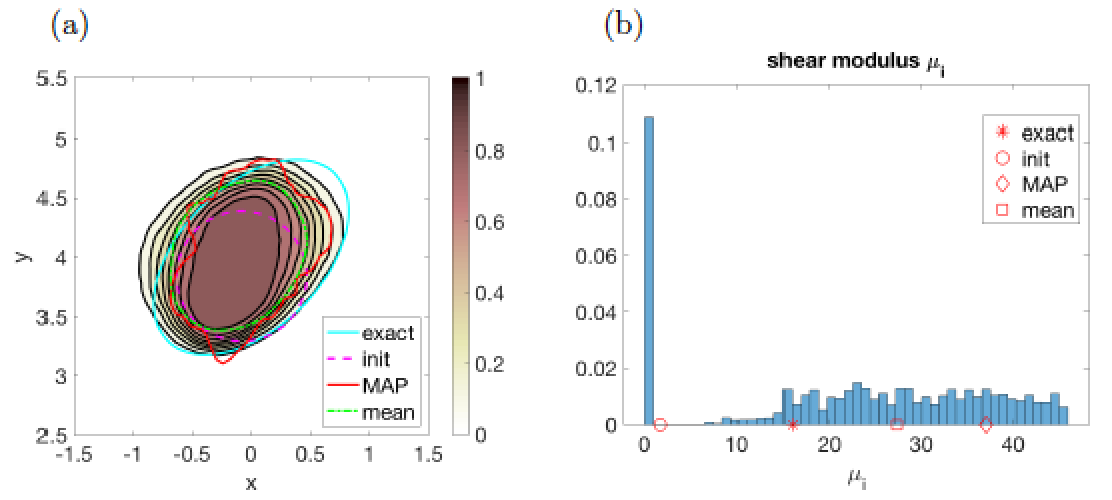
Figure 13: Results for the rotated ellipse, working with high dimensional parametrizations allowing for irregular shapes with $Z=500$. Same sampling parameters as in Fig. 13 except $\tilde{S}=2400$.

Working with smooth shapes, we get Figure 13 for the rotated ellipse already studied in Figure 4(c). The samples we generate behave in a similar way as those in Figure 12(c). The MAP point is unlikely to be smooth when we do not enforce the prior knowledge we have on smoothness. However, the information provided by the mean parameters and the statistics of geometrical characteristics and values for shear moduli is still useful, though less precise. Enforcing a smooth parametrization we get better results for smooth shapes, at a lower computational cost, see Figure 4(c). Similarly, the irregular shape studied in Figure 12 could be studied in the smooth framework employed in Section 5 to obtain information about mean values at a lower cost.

8 Conclusions

We have developed a Bayesian approach for the detection and characterization of anomalies in tissues which uses topological energies to generate priors. In this framework, anomalies are represented by star-shaped objects whose shear moduli differ from the surrounding tissues. We have considered low dimensional parametrizations for simple smooth shapes and higher dimensional approximations for irregular shapes, which can be used to distinguish encapsulated (smooth) and invasive (irregular) tumors, for instance.

For simple shapes, MCMC methods based on different types of affine invariant ensemble samplers provide a good characterization of the structure of the posterior distribution, which displays asymmetric tails for each mode representing an object. This approach is time consuming, since we must generate a few hundred thousand samples by solving a time dependent wave equation for each of them. We have shown that its is possible to approximate the ‘maximum a posteriori’ (MAP) estimate of the parameters defining the hardness and geometry of these anomalies. To do so, we minimize a proper cost functional, which can be done in a few iterations by Newton type iterations. Linearizing the parameter-to-observable map about the MAP point, we are able to quantify the uncertainty in nature of the anomalies, their location and shape by generating samples of the Laplace approximation to the posterior distribution at a low computational cost.

We have tested these schemes in 2D shear imaging set-ups, finding reasonable agreement between both sampling techniques for such shapes. While MCMC sampling furnishes a deeper insight in the structure of the posterior, including asymmetry and possible multimodality, the linearization approach provides results quite fast. This is essential for potential technological applications and three dimensional extensions. However, it may miss multimodality and asymmetry details.

Irregular shapes lead to higher dimensional problems and optimization approaches to calculate a MAP point encounter difficulties due to fast variations in the boundary. We have seen that affine invariant samplers which are robust as dimension grows still provide some information on basic anomaly properties, though we identify multimodality features due to inconsistency between the data and the prior. Better descriptions of the anomaly shape and shear modulus would probably require improved prior knowledge or a different type of parametrization.

Alternative Bayesian formulations seek variations in the wave speed of the whole tissue, which leads to infinite dimensional problems and very large computational cost. The approach based on seeking shapes described by a moderate number of parameters that we propose here has been tried for simple shapes on time independent imaging problems for which efficient boundary element solvers are available. Lacking similar solvers for time dependent wave problems, we have succeeded in developing fast finite element schemes allowing us to implement our Bayesian formulation in terms of parametrized boundaries, at a low computational cost, which is convenient for practical applications.

Appendix A Approximate solutions for the forward problem

We recall here the pertinent existence and regularity result for the forward problem, as well as some discretization details and parameter choices.

A.1 Existence and regularity

In the sequel, $H^{1}$, $H^{2}$ represent the standard Sobolev spaces and $(H^{1})^{\prime}$ is the dual space of $H^{1}$ [1, 6]. $L^{2}$ stands for the usual space of square-integrable functions.

Theorem 1. Let $R$ and $\Omega$ be $C^{1}$ domains, $\Omega\subset R$ . Assume $f\in C^{\infty}(\mathbb{R}^{+})\cup L^{\infty}(\mathbb{R}^{+})$ and $g\in C^{\infty}(\mathbb{R}^{2})\cup L^{\infty}(\mathbb{R}^{2})$. Then, the problem (3)-(6) has a unique solution $u\in C([0,\tau];H^{1}(R))$, $u_{t}\in C([0,\tau];L^{2}(R))$, $u_{tt}\in L^{2}(0,\tau;(H^{1}(R))^{\prime})$, for any $\tau>0$. Furthermore, if $u_{tt}(\mathbf{x},0)=0$, we also have $u_{t}\in C([0,\tau];H^{1}(R))$ and $u\in C([0,\tau];H^{2}(R\setminus\overline{\Omega}))$.

Proof. Existence of a solution $u$ with the stated regularity for wave equations with positive and bounded $\mu$ and $\rho$ is a particular case of results established in [32, 42]. If $u_{tt}(\mathbf{x},0)=0$, $u_{t}$ solves (3)-(6) with $f$ replaced by $f^{\prime}$. Hence, $u_{t}\in C([0,\tau];H^{1}(R))$ and $u_{tt}\in C([0,\tau];L^{2}(R)).$ Then equation (3) implies that $\Delta u(t)\in L^{2}(R\setminus\overline{\Omega})$, thus $u(t)\in H^{2}(R\setminus\overline{\Omega})$ by elliptic regularity theory and $u$ is defined on $\Sigma$ and the receiving sites both in the sense of $L^{2}(\Sigma)$ traces and pointwise [6, 11].

A.2 Physical parameters and nondimensionalization

For computational purposes, we nondimensionalize the problem using characteristic times and lengths. Let $T$ and $L$ be two characteristic time and length scales to be chosen. To simplify, one can take $\rho_{\rm i}=\rho\sim 1000\,\rm kg/m^{3}$ in tissues, though $\rho_{\rm i}>\rho$ in general (slightly). We set $\mathbf{x}=\mathbf{x}^{\prime}L$, $t=t^{\prime}T$, $u=u^{\prime}L$, $\Omega=\Omega^{\prime}L$, $R=R^{\prime}L$ and $\Sigma=\Sigma^{\prime}L$. Making the change of variables and dropping the symbol ^′ for ease of notation, we get

$$\begin{array}[]{ll}u_{tt}-{\rm div}({\mu T^{2}\over\rho L^{2}}\nabla u)={T^{2}\over\rho L}f(tT)G(\mathbf{x}L)=\tilde{f}(t)\tilde{G}(\mathbf{x}),&\mathbf{x}\in R,\;t>0,\\[4.30554pt] {\partial u\over\partial\mathbf{n}}=0,&\mathbf{x}\in\partial R,\\[4.30554pt] u(\mathbf{x},0)=0,u_{t}(\mathbf{x},0)=0,&\mathbf{x}\in R.\end{array}$$ (43)

Here, $\tilde{f}(t)=f_{0}{T^{2}\over\rho L}(1-2\pi^{2}f_{M}^{2}T^{2}t^{2})e^{-\pi^{2}f_{M}^{2}T^{2}t^{2}}$. We choose $\tilde{G}$ to have zero normal derivative at the interface, for instance, $\tilde{G}(\mathbf{x})={1\over(\pi\kappa)^{n/2}}\sum_{j=1}^{J}\exp(-{|(\mathbf{x}-\mathbf{x}_{j})|^{2}\over\kappa})$, $n=2$. This function represents the location of the emitters.

Typical experimental conditions [3, 27, 50] suggest the choice $L=1$ cm = $10^{-2}$ m and $T=10^{-2}$ s. For instance, typical anomaly shapes and sizes in a liver framework are ellipsoids of about $0.963\times 1.15$ cm, buried at a depth between $6$ and $12$ cm. To spot anomalies of size $1$ cm, that is, $10^{-2}$ m, we should need a receiver grid of step about $10^{-3}$ m distributed or moving over regions of cm length. Typical parameter ranges [3, 27, 50] are $\mu_{\rm i}=96-241$ kPa (carcinoma), $\mu_{\rm i}=55-71$ kPa (normal tissue), and $\mu_{\rm i}=36-41$ kPa (bening hyperplasia) in a prostate gland, for instance. In a liver framework, $\mu_{\rm i}=0.4-6$ kPa (healthy tissue) and $\mu_{\rm i}=15-100$ (unhealthy tissue). Breast is less appropriate for these methods because carcinoma may yield $\mu_{\rm i}=22-560$ kPa, ovelapping with fibrous tissue $\mu_{\rm i}=96-244$ kPa, normal fat $\mu_{\rm i}=18-24$ kPa, and normal gland $\mu_{\rm i}=28-66$ kPa, other techniques [30] may be more suitable. Frequencies $f_{M}$ in shear elastography devices are $4-15$ Hz, or $50$ Hz, or $100-300$ Hz, depending on sizes involved.

$L$	$T$	$\rho_{\rm i}$	$\rho$	$\mu_{\rm i}$	$\mu$	$c_{\rm i}$	$c$	$f_{M}$	$f_{0}$
$0.01$ m	$0.01$ s	$\rho$	$10^{3}\rm{kg\over m^{3}}$	$16$ kPa	$1.69$ kPa	$4\rm{m\over s}$	$1.3{m\over s}$	$50$ Hz	${\rho L\over T^{2}}$

Table 1: Dimensional parameters used in the simulations.

In our numerical tests we work with the parameters listed in Table 1. We set $\mu_{\rm i}=16$ kPa and $\mu=1.69$ kPa, which results in wave speeds $c_{\rm i}=4$ m/s inside the anomalies and $c=1.3$ m/s outside, a low contrast situation. We select $f_{0}$ such that $f_{0}{T^{2}\over\rho L}=1$ and $f_{M}=50$ Hz so that $f_{M}T=0.5$. Then, the final dimensionless forward problem is

$$\begin{array}[]{ll}u_{tt}-{\rm div}(c(\mathbf{x})^{2}\nabla u)=\tilde{f}(t)\tilde{G}(\mathbf{x}),&\mathbf{x}\in R,\\[4.30554pt] {\partial u\over\partial\mathbf{n}}=0,&\mathbf{x}\in\partial R,\\[4.30554pt] u(\mathbf{x},0)=0,u_{t}(\mathbf{x},0)=0,&\mathbf{x}\in R,\end{array}$$ (47)

for $t>0$, with

$$c^{2}(\mathbf{x})={\mu(\mathbf{x})T^{2}\over\rho L^{2}}=\left\{\begin{array}[]{ll}1.69,&\mathbf{x}\in R\setminus\overline{\Omega},\\ 16,&\mathbf{x}\in\Omega,\end{array}\right.\quad c(\mathbf{x})=\left\{\begin{array}[]{ll}1.3,&\mathbf{x}\in R\setminus\overline{\Omega},\\ 4,&\mathbf{x}\in\Omega,\end{array}\right.$$

and

$$\tilde{f}(t)\tilde{G}(\mathbf{x})=(1\!-\!2\pi^{2}0.5^{2}t^{2}){e^{-\pi^{2}0.5^{2}t^{2}}\over\pi\kappa}\sum_{j=1}^{J}e^{-{|\mathbf{x}-\mathbf{x}_{j}|^{2}\over\kappa}}.$$ (49)

We generate synthetic data for our simulations by solving numerically (47)-(49) for different choices of anomalies $\Omega$ and adding random noise. We have used finite elements [12, 42] with spatial step $\delta x=0.08$ and a total explicit spatial discretization with time step $\delta t=0.00125$, see next section for details. We locate emitter/receivers at fixed grids of step $0.5$ (or $0.2$) and record the signal at a fixed time grid of step $0.025$. The value of $\kappa$ can be adjusted to the step $\delta x$, so that it affects just a few nodes around the emitter. Here, we have set $\kappa=2$. Alternatively, one could also perform an even extension at the interface $\Sigma=\{(x,y)\,|\,y=0\}$ to get a problem set in the whole space and resort to boundary elements for wave problems [41] representing the emitters as point sources. However, an adequate framework to implement such boundary value approach is still missing.

A.3 Discretization

To reduce the computational cost we focus on a limited tissue region and truncate the computational region in such a way that $R$ is a rectangular region, as in Figure 1. On the artificial boundaries $\partial R\setminus\Sigma$, we will enforce non reflecting boundary conditions [17]. On $\Sigma$, we keep the zero Neuman condition. For the spatial discretization, we use $P_{1}$ finite elements on a fixed mesh of step $\delta x$ in space [12, 42]. If $V={\rm span}\{\phi_{1},\ldots,\phi_{D}\}\subset H^{1}$ is the resulting finite element space, we approximate $u$ by $u^{D}=\sum_{i=1}^{D}a_{i}(t)\phi_{i}$. Therefore, we must find $u^{D}$ such that

$$\int_{R}u^{D}_{tt}(\mathbf{x},t)\phi_{j}(\mathbf{x})d\mathbf{x}+\int_{R}c(\mathbf{x})^{2}\nabla u^{D}(\mathbf{x},t)\phi_{j}(\mathbf{x})d\mathbf{x}-\int_{\partial R\setminus\Sigma}c^{2}{\partial u^{D}\over\partial\mathbf{n}}\phi_{j}(\mathbf{x})dS_{\mathbf{x}}$$

$$=\tilde{f}(t)\int R\tilde{G}(\mathbf{x})\phi_{j}(\mathbf{x})d\mathbf{x},$$

for $j=1,\ldots,D$. Next, we use the nonreflecting boundary condition ${\partial u^{D}\over\partial\mathbf{n}}\sim-{1\over c}u_{t}^{D}$ on $\partial R\setminus\Sigma$ and total discretizations for the time derivatives on a time mesh $t_{n}$ of step $\delta t$ [12, 42]

$$u^{D}_{tt}(\mathbf{x},t_{n})\sim{u^{D}(\mathbf{x},t_{n+1})-2u^{D}(\mathbf{x},t_{n})+u^{D}(\mathbf{x},t_{n-1})\over\delta t^{2}},$$

$$u^{D}_{t}(\mathbf{x},t_{n})\sim{u^{D}(\mathbf{x},t_{n})-u^{D}(\mathbf{x},t_{n-1})\over\delta t}.$$

To calculate the coefficients $a_{i}(t_{n})$, $i=1,\ldots D$, we solve the recurrence relations

$$\sum_{i=1}^{D}M_{j,i}a_{i}(t_{n+1})=\sum_{i=1}^{D}M_{j,i}(2a_{i}(t_{n})-a_{i}(t_{n-1}))-\delta t^{2}\sum_{i=1}^{D}A_{j,i}a_{i}(t_{n})$$

$$-c\,\delta t\sum_{i=1}^{D}B_{j,i}(a_{i}(t_{n})-a_{i}(t_{n-1}))+\delta t^{2}\tilde{f}(t_{n})G_{j},$$

for $n\geq 1$, where $M_{j,i}=\int_{R}\phi_{j}\phi_{i}d\mathbf{x}$, $A_{j,i}=\int_{R}c^{2}\nabla\phi_{j}\nabla\phi_{i}d\mathbf{x}$, $B_{j,i}=\int_{\partial R\setminus\Sigma}\phi_{j}\phi_{i}dS_{\mathbf{x}}$, $G_{j}=\int_{R}\tilde{G}\phi_{j}d\mathbf{x}.$ The coefficients $a_{i}(t_{0})=0$ and $a_{i}(t_{1})=0$ for $i=1,\ldots,D$ are determined using the initial conditions. The numerical solutions defined in this way are continuous, so that the costs (8), (33), likelihoods (16), and topological energies (28) are well defined.

Acknowledgements. This research has been partially supported by the FEDER /Ministerio de Ciencia, Innovación y Universidades - Agencia Estatal de Investigación grants No. MTM2017-84446-C2-1-R and PID2020-112796RB-C21. AC thanks G. Stadler for nice discussions and useful suggestions.

References

- [1] Adams R A 1975 Sobolev Spaces (Academic Press, New York)
- [2] Afkham B M, Dong Y and Hansen P C 2021 Uncertainty quantification of inclusion boundaries in the context of X-ray tomography, arXiv:2107.06607v1.
- [3] Shear Wave Elastography, in Blumgart’s Surgery of the Liver, Biliary Tract and Pancreas, 2-Volume Set (Sixth Edition), 2017.
- [4] Bui-Thanh T and Ghattas O 2014 An analysis of infinite dimensional Bayesian inverse shape acoustic scattering and its numerical approximation SIAM/ASA J. Uncertain. Quantification 2 203-22
- [5] Bui-Thanh T, Ghattas O, Martin J and Stadler G 2013 A computational framework for infinite-dimensional Bayesian inverse problems Part I: The linearized case with application to global seismic inversion SIAM J. Sci. Comput. 35 A2494-A2523
- [6] Brézis H 1987 Analyse fonctionnelle Théorie et applications (Paris: Masson)
- [7] Carpio A and Rapún ML 2012 Hybrid topological derivative and gradient-based methods for electrical impedance tomography Inverse Problems 28 095010
- [8] Carpio A, Dimiduk TG, Le Louër F and Rapún ML 2019 When topological derivatives met regularized Gauss-Newton iterations in holographic 3D imaging J. Comp. Phys. 388 224-251
- [9] Carpio A, Iakunin S and Stadler G 2020 Bayesian approach to object detection with topological priors Inverse Problems 36 105001
- [10] Colton D and Kress R 1998 Inverse Acoustic and Electromagnetic Scattering (Berlin: Springer)
- [11] Cazenave T and Haraux A 1999 An introduction to semilinear evolution equations Oxford Lecture Series in Mathematics and Its Applications 13 (Oxford: Clarendon Press)
- [12] Dautray R and Lions L 1984-87 Analyse mathématique et calcul numérique pour les sciences et les techniques (Paris: Masson)
- [13] Dominguez N, Gibiat V and Esquerre Y 2005 Time domain topological gradient and time reversal analogy: an inverse method for ultrasonic target detection Wave Motion 42 31-52,
- [14] Dominguez N and Gibiat V 2010 Non-destructive imaging using the time domain topological energy method Ultrasonics 50 367-372
- [15] Dunlop M M 2016 Analysis and computation for Bayesian inverse problems PhD Thesis Warwick
- [16] Dunlop M M and Stadler G 2022 A gradient-free subspace-adjusting ensemble sampler for infnite-dimensional Bayesian inverse problems, arXiv:2202.11088v1
- [17] Engquist B and Majda A 1979 Radiation boundary conditions for acoustic and elastic wave calculations Commun. Pur. Appl. Math. 32 312-358
- [18] Engquist B, Froese B D and Yang Y 2016 Optimal transport for seismic full waveform inversion Comm. Math. Sci. 14 2309-2330
- [19] Fletcher R 1971 Modified Marquardt subroutine for non-linear least squares Tech. Rep. 197213
- [20] Fichtner A, Bunge H P and Igel H 2006 The adjoint method in seismology - II Applications: traveltimes and sensitivity functionals Physics of the Earth and Planetary interiors 157 105-123
- [21] Harbrech H and Hohage T 2007 Fast methods for three-dimensional inverse obstacle scattering problems J. Integral Equ. Appl. 19 237-260
- [22] Gebraad L, Boehm C and Fichtner A 2020 Bayesian elastic full-waveform inversion using Hamiltonian Monte Carlo JGR Solid Earth 125 e2019JB018428
- [23] Goodman J and Weare J 2010 Ensemble samplers with affine invariance, Commun. Appl. Math. Comput. Sci. 5 65-80
- [24] Guo Z and De Hoop M V, 2012 Shape optimization in full waveform inversion with sparse blocky model representations Proceedings of the Project Review, Geo-Mathematical Imaging Group (Purdue University, West Lafayette IN) 1 189-208
- [25] Guzina B and Chikichev I 2007 From imaging to material identification: a generalized concept of topological sensitiviy J. Mech. Phys. Solids 55 245-279
- [26] Hohage T and Schormann C 1998 A Newton-type method for a transmission problem in inverse scattering Inverse Problems 1, 1207-27
- [27] Hoyt K, Castaneda B, Zhang M, Nigwekar P, di Sant’Agnese P A, Joseph J V, Strang J, Rubens D J and Parker K J 2008 Tissue elasticity properties as biomarkers for prostate cancer Cancer Biomark. 4 213-225
- [28] Kaipio J and Somersalo E 2006 Statistical and computational inverse problems Vol 160 (Berlin: Springer)
- [29] Käuf P, Fichtner A and Igel H 2010 Object-based probabilistic full-waveform tomography Master thesis Geophysics LMU Munchen
- [30] Korta Martiartu N, Boehm C, Vinard N, Jovanovic Balic I and Fichtner A 2017 Optimal experimental design to position transducers in ultrasound breast imaging Medical Imaging Ultrasonic Imaging and Tomography 10139, 101390M, International Society for Optics and Photonics
- [31] Landau L D and Lifshitz L M 1986 Theory of elasticity (Oxford: Butterworth-Heinemann 3rd Edition)
- [32] Lions J L and Magenes E 1968 Problémes aux limites non homogénes (Paris: Dunod)
- [33] Medical Imaging Systems: An Introductory Guide 2018 Maier A, Steidl S, Christlein V, J Hornegger (Eds.) Springer
- [34] Malcolm A and Guzina B 2008 On the topological sensitivity of transient acoustic fields Wave Motion 45 821-834
- [35] Métivier L, Brossier R, Mérigot Q, Oudet E and Virieux J 2016 Measuring the misfit between seismograms using an optimal transport distance: application to full waveform inversion Geophys. J. Int. 205 345-377
- [36] Mishra A 2017 Hologram the future of medicine - From Star Wars to clinical imaging Indian Heart J. 69 566-567
- [37] Neal R M 2011 MCMC using Hamiltonian dynamics. In: Brooks S, Gelman A, Jones GL, Meng XL, editors. Handbook of Markov chain Monte Carlo (London: Chapman & Hall)
- [38] Nec̆as J 1983 Introduction to the theory of nonlinear elliptic equations (Leipzig: Teubner)
- [39] Palafox A, Capistrán M A and Christen J A 2017 Point cloud-based scatterer approximation and affine invariant sampling in the inverse scattering problem Math. Methods Appl. Sci. 40 3393-403
- [40] Petra N, Martin J, Stadler G and Ghattas O 2014 A computational framework for infinite-dimensional Bayesian inverse problems: Part II. Stochastic Newton MCMC with application to ice sheet flow inverse problems SIAM J. Sci. Comput. 36 A1525-55
- [41] Hsiao G C, Sánchez-Vizuet T and Sayas F J 2017 Boundary and coupled boundary-finite element methods for transient wave-structure interaction IMA Journal of Numerical Analysis 37 237-265
- [42] Raviart P A and Thomas J M 1983 Introduction a l’analyse numérique des équations aux dérivées partielles (Paris: Masson)
- [43] Rasmussen C E and Williams C K I 2006 Gaussian Processes for Machine Learning (MIT Press)
- [44] Sahuguet P, Chouippe A and Gibiat V 2010, Biological tissues imaging with Time Domain Topological Energy, Physics Procedia 3 677-683
- [45] Sandrin L, Tanter M, Catheline S and Fink M 2002 Shear modulus imaging with 2-D transient elastography, IEEE transactions on ultrasonics, ferroelectrics, and frequency control 49 426-435
- [46] Sarvazyan A P, Urban M W and Greenleaf J F 2013 Acoustic waves in medical imaging and diagnostics Ultrasound Med. Biol. 39 1133-46
- [47] Sarvazyan A, Hall TJ, Urban MW, Fatemi M, Aglyamov SR and Garra BS 2011 Overview of elastography - an emerging branch of medical imaging Current Medical Imaging Reviews 7 255-282
- [48] Tarantola A 2005 Inverse Problem Theory and Methods for Model Parameter Estimation (Philadelphia PA: SIAM)
- [49] Tsogka C and Papanicolaou G C 2002 Time reversal through a solid-liquid interface and super-resolution Inverse Problems 18 1639-1657
- [50] Wang Y, Yao B, Li H, Zhang Y, Gao H, Gao Y, Peng R and Tang J 2017 Assessment of tumor stiffness with shear wave elastography in a human prostate cancer xenograft implantation model J Ultrasound Med 36 955-963
- [51] Zhu H, Li S, Fomel S, Stadler G and Ghattas O 2016 A Bayesian approach to estimate uncertainty for full-waveform inversion using a priori information from depth migration Geophysics 81 R307-R323