A machine learning study to identify collective flow in small and large colliding systems

Abstract

Collective flow has been found similar between small colliding systems (p+p and p+A collisions) and large colliding systems (peripheral A+A collisions) at the CERN Large Hadron Collider (LHC). In order to study the difference of collective flow between small and large colliding systems, we employ a point cloud network to identify $p$ $+$ Pb collisions and peripheral Pb $+$ Pb collisions at $\sqrt{s_{NN}}=$ 5.02 TeV from a multiphase transport model (AMPT). After removing the discrepancies in the pseudorapidity distribution and the $p_{\rm T}$ spectra, we capture the discrepancy in anisotropic flow. Although the verification accuracy of our PCN is limited due to similar event-by-event distributions of elliptic and triangular flow, we demonstrate that collective flow between $p$ $+$ Pb collisions and peripheral Pb $+$ Pb collisions becomes more different with increasing final hadron multiplicity and parton scattering cross section.

I INTRODUCTION

Quark-gluon plasma (QGP) at extreme conditions of high temperature and density is thought to be a form of the early universe, which has been produced in the laboratory by relativistic heavy-ion collisions at the BNL Relativistic Heavy Ion Collider (RHIC) and the CERN Large Hadron Collider (LHC) Adams et al. (2005); Adcox et al. (2005); Aamodt et al. (2008); Bzdak et al. (2020); Luo and Xu (2017). The experimental results have shown that this new type of strongly interacting matter behaves as a perfect fluid, because it translates initial spatial geometry or initial energy density fluctuations into momentum anisotropy of the final particles through pressure gradients in hydrodynamics with the smallest ratio of shear viscosity over entropy Heinz and Snellings (2013); Song and Heinz (2008); Jeon and Heinz (2015); Shen and Yan (2020); Gale et al. (2013); Yan (2018); Alver and Roland (2010); Ma and Wang (2011); Yan et al. (2014); Qin et al. (2010), thus generating strong collective flow Ollitrault (1992); Stoecker (2005).

Over the last decade, the measurements of collective flow in various colliding systems, such as $p$$+$$p$, $p$$+$Pb collisions at the LHC Khachatryan et al. (2010); Chatrchyan et al. (2013); Abelev et al. (2013a); Aad et al. (2013a); Sirunyan et al. (2018); Acharya et al. (2019), $p$$+$Au, $d$$+$Au, and ³He$+$Au collisions at RHIC Adare et al. (2015); Adamczyk et al. (2015); Aidala et al. (2019); Acharya et al. (2022); Abdulameer et al. (2023), have been performed. Surprisingly, similar collective flow is found in peripheral A+A and high multiplicity $p$+A collisions at the same multiplicity, raising doubts about whether QGP droplets can be also generated in small colliding systems. Many theoretical efforts have been made to understand the origin of collective flow in small colliding system Dusling et al. (2016); Loizides (2016); Nagle and Zajc (2018). Basically, they can be divided into two categories depending on whether the origin is from the initial or final state. The color glass condensate (CGC) in the initial state has also been proposed as a possible mechanism to interpret the experimentally measured “flow” in small colliding systems Dumitru et al. (2011); Dusling and Venugopalan (2013); Skokov (2015); Schenke et al. (2015); Schlichting and Tribedy (2016); Kovner et al. (2017); Iancu and Rezaeian (2017); Mace et al. (2018); Nie et al. (2019); Shi et al. (2021). Similarly to large colliding systems, hydrodynamics in final sate also can transform the initial geometric asymmetry into the final momentum anisotropic flow through the pressure gradient of the QGP in small colliding systems Bozek (2012); Bzdak et al. (2013); Shuryak and Zahed (2013); Qin and Müller (2014); Bozek and Broniowski (2013); Bozek et al. (2015); Song et al. (2017). It is generally believed that the transport model will behave more like hydrodynamics as the multiplicity or scattering cross section increases, i.e., from non-equilibrium to equilibrium. It has been demonstrated that a Multi-Phase Transport (AMPT) model Lin et al. (2005) is capable of describing the experimental data in both large and small colliding systems Bzdak and Ma (2014); Orjuela Koop et al. (2015); Ma and Bzdak (2016). Since most of partons are not scattered in the small colliding systems at RHIC and the LHC, a parton escape mechanism has been proposed to explain the formation of azimuthal anisotropies in the transport model He et al. (2016); Lin et al. (2016). It has been shown that parton collisions are crucial for the generation of anisotropic flows Ma and Bzdak (2016); Ma et al. (2021). By using a new test-particle method, we recently proved that collectivity established by final state parton collisions is much stronger in large colliding systems compared to that in small colliding systems Wang and Ma (2022).

On the other hand, the event-averaged flow $v_{n}$ mainly reflects the averaged hydrodynamic response to the initial collision geometry of the produced matter. More information, such as the event-by-event (EbyE) fluctuations of the overlap region Alver and Roland (2010), can be obtained by measuring event-by-event $v_{n}$ distribution $P(v_{n})$ for charged hadrons, which has been measured by the ATLAS Collaboration using unfolding method in Pb$+$Pb collisions at $\sqrt{s_{NN}}$ = 2.76 TeV Aad et al. (2013b), which gives a good constraint to the initial condition in A+A collisions. However, the corresponding experimental measurements in small colliding systems are not yet available.

In addition to the similarity of the anisotropic flow $v_{n}$, the differences of other observables are worthy of investigation between large and small colliding systems, such as pseudorapidity distribution and $p_{\rm T}$ spectra. For example, previous experimental studies have shown power law-shaped $p_{\rm T}$ spectra in small colliding systems Adams et al. (2006); Abelev et al. (2014); Adam et al. (2015); Acharya et al. (2020); Abelev et al. (2009, 2013b), unlike exponential-shaped $p_{\rm T}$ spectra in large colliding systems Adcox et al. (2004); Abelev et al. (2009, 2013b).

With the advancement of computational hardware and algorithms, machine learning (ML) techniques have become a popular and powerful tool for extracting information from big data, and has been applied in high energy nuclear physics for various topics Pang et al. (2018); Zhou et al. (2019); Graczykowski et al. (2022); ZHOU et al. (2022); WANG et al. (2022); HE et al. (2022); DU et al. (2022); LI et al. (2023). Among many deep neural network architectures within ML, the point cloud network (PCN) is a highly efficient and effective architecture that can solve many problems by involving point cloud structured record, such as 3D object segmentation and scene semantic parsing Qi et al. (2016). It has also been used in high energy nuclear physics, such as reconstructing the impact parameter of collisions precisely Steinheimer et al. (2019); Omana Kuttan et al. (2020a); Omana Kuttan et al. (2021), classifying the equation of state (EOS) Omana Kuttan et al. (2020b), and identifying weak intermittency signals associated with critical phenomena Huang et al. (2022) by learning the data for heavy-ion collisions. In this work, by adopting PCN in supervised training, we will find out if it is possible to distinguish between $p$$+$Pb collisions and peripheral Pb$+$Pb collisions from the multiphase transport (AMPT) model, and reveal the differences between small and large colliding systems.

The paper is organized as follows. First, we introduce the AMPT model, which generates the data for $p$$+$Pb collisions and peripheral Pb$+$Pb collisions, and the relevant observables in Sec. II. In Sec. III, we describe the details of the PCN. In Sec. IV, the validation accuracy of PCN is presented and the relevant physics is discussed. Finally, we summarize the implications of our results in Sec. V.

II MODEL AND METHOD

II.1 A multiphase transport model

The string melting version of AMPT model consists of four main stages of heavy-ion collisions, i.e. initial state, parton cascade, hadronization, and hadronic rescatterings. The initial state with fluctuating initial conditions is generated by the heavy ion jet interaction generator (HIJING) model Gyulassy and Wang (1994). In HIJING model, minijet partons and excited strings are produced by hard processes and soft processes, respectively. In the string melting mechanism, all excited hadronic strings in the overlap volume are converted to partons according to the flavor and spin structures of their valence quarks Lin and Ko (2002). The partons are generated by string melting after a formation time:

$$t_{f}=E_{H}/m^{2}_{T,H},$$ (1)

where $E_{H}$ and $m_{T,H}$ represent the energy and transverse mass of the parent hadron. The initial positions of partons originating from melted strings are determined by tracing their parent hadrons along straight-line trajectories. The interactions among partons are described by the Zhang’s parton cascade (ZPC) model Zhang (1998), which includes only two-body elastic scatterings with a g+g $\rightarrow$ g+g cross section, i.e.,

$$\frac{d\sigma}{d\hat{t}}=\frac{9\pi\alpha^{2}_{s}}{2}(1+\frac{\mu^{2}}{\hat{s}})\frac{1}{(\hat{t}-\mu^{2})^{2}},$$ (2)

where $\alpha_{s}$ is the strong coupling constant (taken as 0.33), while $\hat{s}$ and $\hat{t}$ are the usual Mandelstam variables. The effective screening mass $\mu$ is taken as a parameter in ZPC for adjusting the parton scattering cross section. Note that previous AMPT model studies have shown that a parton scattering cross section of 3 mb can well describe both large and small colliding systems at RHIC and the LHC energies Lin (2014); Orjuela Koop et al. (2015); Ma and Bzdak (2016); Ma and Lin (2016); He and Lin (2017); Lin and Zheng (2021). A quark coalescence model is used for hadronization at the freeze out of parton system. The hadronic scatterings in hadronic phase are simulated by a relativistic transport (ART) model Li and Ko (1995).

In this study, we simulated 2 million events each for peripheral Pb$+$Pb collisions and $p$$+$Pb minimum bias collisions at $\sqrt{s_{NN}}$ = 5.02 TeV, using a string-melting version of the AMPT model with parton scattering cross sections of 0 mb, 3 mb, and 10 mb, respectively.

II.2 Anisotropic flow

To quantify the azimuthal anisotropy $v_{n}$ in final momentum space, the azimuthal angle distribution of measured particles can be decomposed into a Fourier series,

$$\frac{{\rm d}N}{{\rm d}\phi}=\frac{1}{2\pi}\Bigg{[}1+\sum_{n=1}^{\infty}2v_{n}\cos{\left(n(\phi-\psi_{n})\right)}\Bigg{]},$$ (3)

where $\phi$ is the azimuthal angle, $\psi_{n}$ is the $n^{\rm th}$ harmonic event plane angle, $v_{n}=\langle\cos{[n(\phi-\psi_{n})]}\rangle$ is the $n^{\rm th}$ order of harmonic flow coefficient Voloshin and Zhang (1996). The second ($v_{2}$) and third ($v_{3}$) Fourier coefficients represent the amplitude of elliptic and triangular flow, respectively. The linearized hydrodynamic response shows that anisotropy flow $v_{n}$ is correlated to the geometry asymmetry of energy density profile in spatial space of initial state, namely the initial eccentricity $\varepsilon_{n}$,

$$\varepsilon_{n}=\frac{\sqrt{\langle r^{n}\cos(n\phi_{r})\rangle^{2}+\langle r^{n}\sin(n\phi_{r})\rangle^{2}}}{\langle r^{n}\rangle},$$ (4)

where $r$ and $\phi_{r}$ are the polar coordinates of participating nucleons Alver and Roland (2010). In hydrodynamics, harmonic flows are responding to eccentricities,

$$v_{n}=v_{n}(\varepsilon_{n},k),$$ (5)

where the constant $k$ is sensitive to the properties of the QGP, such as the transport coefficient $\eta/s$ Yan (2018).

Figure 1: The architecture of the devised point cloud network (PCN). In this network, it takes final state $N$ points as input, applies input and feature transformations, and then aggregates point features by max-pooling. The output is classification scores for 2 classes, i.e., the probability of Pb$+$Pb or $p$$+$Pb colliding systems.

On the other hand, the EbyE distribution of $v_{n}$, P($v_{n}$), can be obtained by an unfolding method, which suppresses the nonflow contribution. However, there is some problem with the unfolding process for small systems. For $p+A$ systems, the response matrix in the unfolding method can not be obtained reliably. For example, there is no convergent result in p+p system. Therefore, the unfolding method is not used in this paper.

III Training the PCN for classifying two systems

In this section, we introduce the detailed analysis procedures, including the input and output, the PCN architecture, training, and evaluation of the PCN.

III.1 Input to the machine

The AMPT events for both $p$$+$Pb and Pb$+$Pb collisions are grouped into the data sets according to the number of final charged particles $N_{ch}$ measured in the kinetic window of $|\eta|<$ 2.4 and $p_{\rm T}>$ 0.4 GeV/c. These data are divided into various centrality classes for the colliding systems, which are the $N_{ch}$ bins of 60-90, 90-120, 120-150, 150-185, 185-230. Each data set has about 0.2 million events which are separated into training events and validation events by a ratio of 70% to 30%. All the information about the final state particles within $|\eta|<$ 2.4 in each event are the input to the PCN as a sample, which consists of a list of particles with their information on ($p_{\rm x}$, $p_{\rm y}$, $p_{z}$, $E$) or ($p_{\rm x}$, $p_{\rm y}$). Simultaneously, the two true labels, $p$$+$Pb and Pb$+$Pb, are marked on each event to perform the supervised training.

III.2 Network architecture

The architecture of PCN is shown in Fig.1. It begins with an input alignment network. The following are a shared pointwise multilayer perceptron (MLP) implemented by 1D-convolution neural network (CNN) to extract 32 feature maps, a feature alignment network, a shared MLP to extract 32, 64 and 512 feature maps, respectively. A global max pooling then gets the maximum values of each feature among all particles as one global feature of the particle cloud. Finally, a shared MLP implemented by 3 layers fully connected deep neural network (DNN) with 256, 128, and 2 neurons tags each event as $p$$+$Pb or Pb$+$Pb collision. Batch normalization layers are present between every convolution layer. The LeakyReLU($\alpha$=0.01) activation function is used for all layers except the final layer. The sigmoid activation is used on the final layer for binary classification. The models use the Adam optimizer with a learning rate of $10^{-4}$ with total decay $10^{-4}$ and categorical cross entropy as the loss function. In addition, a dropout layers (with drop out probability 0.3) and L2 regularization are present to tackle the overfitting issue. We use a maximum of 50 epochs with 32 batch size to train the data set.

IV Training results and discussion

In our study, two cases of input data have been investigated. In the case 1, the input for training is an EbyE list of four-momentum ($p_{\rm x}$, $p_{\rm y}$, $p_{z}$, $E$) of the selected final state hadrons from the AMPT model. The input data have a dimension of $N\times 4$, where $N$ is the maximum number of selected particles in an event. Events with fewer particles are filled with zeros to maintain the same input dimension. The case 2 is the same as the case 1, but the input is a list of two-momentum ($p_{\rm x}$, $p_{\rm y}$) of selected final state hadrons.

IV.1 Case 1: training with four-momentum of final hadrons

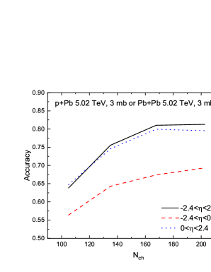
Figure 2: (Color online) Validation accuracy as a function of the number of charged particles $N_{ch}$ by training with four-momentum ($p_{\rm x}$, $p_{\rm y}$, $p_{z}$, $E$) of final particles in pseudorapidity ranges -2.4$<\eta<$2.4 (solid curve), -2.4$<\eta<$0 (dashed curve), and 0$<\eta<$2.4 (dotted curve).

Figure 2 shows validation accuracy as a function of the number of charged particles $N_{ch}$ by learning four-momentum ($p_{\rm x}$, $p_{\rm y}$, $p_{z}$, $E$) of final particles in three different pseudorapidity ranges. All the validation accuracies increase as the multiplicity increases, which indicates that the two colliding systems are more distinguishable for the events with higher multiplicity. The validation accuracies are very close for the pseudorapidity ranges of -2.4$<\eta<$2.4 and 0$<\eta<$2.4. However, there are about 10% drops in validation accuracy for the pseudorapidity range of -2.4$<\eta<$0 relative to the above two cases. This indicates the discrepancy between the two colliding systems mainly comes from the difference in the forward pseudorapidity range, which is the proton-going direction in $p+$Pb systems.

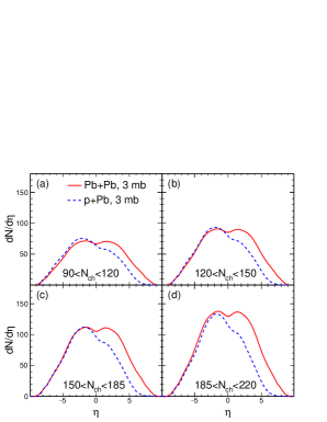
Figure 3: (Color online) The pseudorapidity distributions of final hadrons for different $N_{ch}$ classes in Pb$+$Pb collisions (solid curve) and $p$ $+$ Pb collisions (dashed curve).

To find why the validation accuracy is sensitive to the pseudorapidity range, Fig. 3 compares the pseudorapidity distributions of final hadrons in Pb$+$Pb collisions and $p$$+$Pb collisions for different $N_{ch}$ classes. Between Pb$+$Pb and $p$ $+$ Pb systems, there is a significant difference in the pseudorapidity distribution due to the lower hadron yield in $p$ beam (forward) direction for $p$$+$Pb collisions. This leads to the discrepancy in the above validation accuracies when considering different pseudorapidity ranges. Since the difference in the pseudorapidity distribution in the forward direction becomes more significant at larger $N_{ch}$, it explains why the validation accuracy increases with multiplicity when we train PCN by learning the four-momentum of final particles in Fig.2.

IV.2 Case 2: training with two-momentum of final hadrons

To investigate whether the PCN can learn the difference of collective flow between $p+$Pb collisions and peripheral Pb$+$Pb collisions, three scenarios of lists are used as training inputs, i.e., two-momentum ($p_{\rm x}$, $p_{\rm y}$), normalized two-momentum ($p_{\rm x}^{\rm norm}$, $p_{\rm y}^{\rm norm}$), and normalized meanwhile randomly rotated two-momentum ($p_{\rm x}^{\rm norm,rand}$, $p_{\rm y}^{\rm norm,rand}$), respectively. The normalized two-momentum $p_{\rm x}^{\rm norm}$ and $p_{\rm y}^{\rm norm}$ are defined as,

$$p_{\rm x}^{\rm norm} = \frac{p_{\rm x}}{p_{\rm T}},$$

$$p_{\rm y}^{\rm norm} = \frac{p_{\rm y}}{p_{\rm T}},$$ (6)

where $p_{\rm T}$ is the transverse momentum of each particle. The randomly rotated two-momentum $p_{\rm x}^{\rm rand}$ and $p_{\rm y}^{\rm rand}$ are,

$$p_{\rm x}^{\rm rand} = p_{\rm x}\times\cos{\phi_{\rm rand}}-p_{\rm y}\times\sin{\phi_{\rm rand}},$$

$$p_{\rm y}^{\rm rand} = p_{\rm x}\times\sin{\phi_{\rm rand}}-p_{\rm y}\times\cos{\phi_{\rm rand}},$$ (7)

where $\phi_{\rm rand}$ is a random angle between 0 and 2$\pi$. While, the normalized and randomly rotated two-momentum $p_{\rm x}^{\rm norm,rand}$ and $p_{\rm y}^{\rm norm,rand}$ are,

$$p_{\rm x}^{\rm norm,rand} = \frac{p_{\rm x}\times\cos{\phi_{\rm rand}}-p_{\rm y}\times\sin{\phi_{\rm rand}}}{p_{\rm T}},$$

$$p_{\rm y}^{\rm norm,rand} = \frac{p_{\rm x}\times\sin{\phi_{\rm rand}}-p_{\rm y}\times\cos{\phi_{\rm rand}}}{p_{\rm T}}.$$ (8)

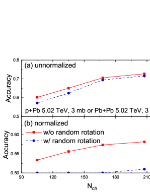
Figure 4: (Color online) Validation accuracy as a function of the number of charged particles $N_{ch}$ by learning with input to be two-momentum ($p_{\rm x}$, $p_{\rm y}$) (a) and the normalized two-momentum ($p_{\rm x}^{\rm norm}$, $p_{\rm y}^{\rm norm}$) (b), each without (solid curve) or with (dashed curve) random rotations.

Figure 4(a) shows validation accuracy as a function of the number of final charged particles $N_{ch}$ with input to be two-momentum ($p_{\rm x}$, $p_{\rm y}$) and its random rotation ($p_{\rm x}^{\rm rand}$ and $p_{\rm y}^{\rm rand}$) of final particles. Validation accuracy of two-momentum input is over $60\%$, and it will drop less than $2\%$, if two-momentum are randomly rotated. It indicates that beside anisotropic flow there is other discrepancy between the two colliding systems, like in $p_{\rm T}$ distributions. To eliminate the effect from different $p_{\rm T}$ distribution of hadron, we train the PCN with normalized two-momentum ($p_{\rm x}^{\rm norm}$, $p_{\rm y}^{\rm norm}$) and its random rotation ($p_{\rm x}^{\rm norm,rand}$ and $p_{\rm y}^{\rm norm,rand}$) of final particles. The validation accuracy as a function of the number of final charged particles is shown in Fig.4(b). Compared to the two-momentum training, there is more than $10\%$ decrease of validation accuracy by learning two-momentum after normalization, which indicates that $p_{\rm T}$ distribution of hadrons is the main feature that distinguishes the two colliding systems, if we train the PCN by two-momentum. Furthermore, the PCN can not distinguish the two colliding systems by learning normalized two-momentum with random rotations of final hadrons, because these operations eliminate the information about the magnitude of $p_{\rm T}$ and anisotropic flow. Compared to the training by the normalized two-momentum with random rotations, the validation accuracy is improved by a few percentages by learning two-momentum with the normalization only. This discrepancy comes from the difference of anisotropic flow between two colliding systems. However, the anisotropic flow between two colliding systems is so similar that the PCN can not distinguish between different colliding systems very well, even though it is better than the case with random rotations.

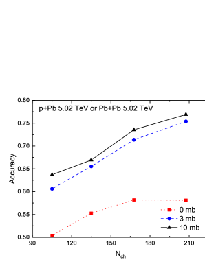
Figure 5: (Color online) Validation accuracy as a function of the number of charged particles $N_{ch}$ by learning two-momentum ($p_{\rm x}$, $p_{\rm y}$) of final hadrons in the AMPT model with different parton cross sections.

Figure 5 shows validation accuracy as a function of the number of final charged particles $N_{ch}$ by learning two-momentum ($p_{\rm x}$, $p_{\rm y}$) of final particles with different parton cross sections. It can be seen that all validation accuracies increase with the increase of $N_{ch}$ and parton cross section. In addition, the PCN can not distinguish the two colliding systems with 0 mb parton cross section at low $N_{ch}$. These results can basically be explained by Fig. 6, since the average transverse momentum $\left\langle p_{\rm T}\right\rangle$ can quantify the feature of $p_{\rm T}$ spectra shape.

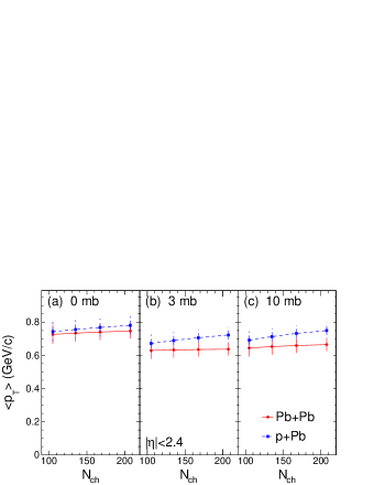
Figure 6: (Color online) Average transverse momenta $\left\langle p_{\rm T}\right\rangle$ in Pb $+$ Pb collisions (solid curve) and p $+$ Pb collisions (dashed curve) as a function of the number of charged particles $N_{ch}$ with parton cross section of 0 mb (a), 3 mb (b), and 10 mb (c).

Figure 6 shows average transverse momenta $\left\langle p_{\rm T}\right\rangle$ as a function of the number of final charged particles $N_{ch}$ with different parton cross sections. We can see that the $\left\langle p_{\rm T}\right\rangle$ in p $+$ Pb collisions is larger than that in Pb $+$ Pb collisions, and the difference is more significant with a larger parton cross section and higher multiplicity. Although we observe that the difference of $\left\langle p_{\rm T}\right\rangle$ is almost zero for 0 mb parton cross section, some validation accuracies are larger than 0.5 for 0 mb in Fig. 5. It indicates that there is a difference of non-flow effect between small and large colliding systems. It could be attributed to jets, because the effects of the jet transverse momentum broadening and multiple scatterings Leonidov et al. (1997) have been found to be stronger in p $+$ Pb collisions than in peripheral Pb $+$ Pb collisions Abelev et al. (2009).

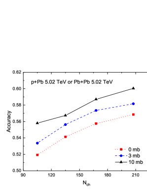
Figure 7: (Color online) Validation accuracy as a function of the number of charged particles $N_{ch}$ by learning normalized two-momentum ($p_{\rm x}^{\rm norm}$, $p_{\rm y}^{\rm norm}$) of final hadrons in the AMPT model with different parton cross sections.

Figure 7 shows validation accuracy as a function of the number of final charged particles $N_{ch}$ by learning normalized two-momentum ($p_{\rm x}^{\rm norm}$, $p_{\rm y}^{\rm norm}$) of final particle with different parton cross sections. It can be seen that the validation accuracy with 0 mb is close to the corresponding result in Fig. 5, and both of them increase with $N_{ch}$, which indicates that the discrepancy of non-flow effect between the two systems is larger for higher multiplicity. However, the discrepancy between 0 mb and nonzero parton cross sections must come from anisotropic flow. The discrepancy increases with parton cross section, which indicates that there is larger discrepancy of anisotropic flow between two colliding systems due to more parton collisions.

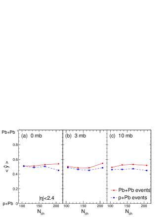
Figure 8: (Color online) Averaged output $\left\langle\widehat{y}\right\rangle$ of the ensembles of two systems identified by the model trained by normalized two-momentum ($p_{\rm x}^{\rm norm}$, $p_{\rm y}^{\rm norm}$) of final hadrons in the AMPT model with different parton cross sections.

If an event is identified as $p$$+$Pb or Pb $+$ Pb, it is marked by the output of $\widehat{y}$=0 or 1, respectively, in our analysis. Thus the averaged output $\left\langle\widehat{y}\right\rangle$ of our model can represent the probability of Pb $+$ Pb of a event. In other words, The closer the $\left\langle\widehat{y}\right\rangle$ is to 0, the more likely the events are $p$$+$Pb collisions, and vice versa for Pb $+$ Pb collisions. Figure 8 shows the averaged output $\left\langle\widehat{y}\right\rangle$ of the ensembles of each system identified by the model trained by normalized two-momentum ($p_{\rm x}^{\rm norm}$, $p_{\rm y}^{\rm norm}$) of final hadrons in the AMPT model with different parton cross sections. It can been seen that $\left\langle\widehat{y}\right\rangle$ of the ensembles of Pb $+$ Pb events is larger than that for $p$$+$Pb events in every situation, which indicates that the PCN is able to distinguish two different ensembles of systems, according to the difference of averaged anisotropic flow between two systems.

To investigate the relationship between anisotropic flow and parton cross section, we further calculate the harmonic flow coefficients, e.g., elliptic flow $v_{2}$, by fitting the long range part of the two-particle azimuthal correlation function $C(\Delta\phi)$, which defined as

$$C(\Delta\phi)=\frac{Y_{same}(\Delta\phi)}{Y_{mixed}(\Delta\phi)}\times\frac{\int Y_{mixed}(\Delta\phi)d\Delta\phi}{\int Y_{same}(\Delta\phi)d\Delta\phi},$$ (9)

where $Y_{same}(\Delta\phi=\phi_{2}-\phi_{1})$ and $Y_{mixed}(\Delta\phi)$ are the number of particle pairs at a given $\Delta\phi$ and within a given $p_{\rm T}$ range for the same and mixed events. This definition of $C(\Delta\phi)$ removes a trivial dependence on the number of produced particles Adler et al. (2006); Adare et al. (2015); Bzdak and Ma (2014).

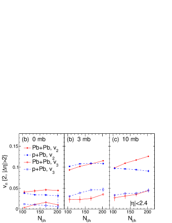
Figure 9: (Color online) Integrated elliptic $v_{2}$ and triangular $v_{3}$ flow coefficient in Pb $+$ Pb collisions (solid curve) and p $+$ Pb collisions (dashed curve) as a function of the number of charged particles $N_{ch}$ with parton cross section of 0 mb (a), 3 mb (b), and 10 mb (c).

Figure 9 shows $v_{2}$ and $v_{3}$ as a function of the number of final charged particles $N_{ch}$ with different parton cross sections. It can be observed that $v_{2}$ and $v_{3}$ increases with parton cross section for Pb$+$Pb collisions. But the dependence on parton cross section is non-monotonous for $p$$+$Pb collisions, which has already been found in Ref. Zhao et al. (2023). It indicates that collective flow can be not only built up but also damaged by the parton collisions in small colliding systems Wang and Ma (2022). The most significant difference of $v_{2}$ between the two systems appears when parton cross section is taken as 10 mb for high-multiplicity events, because there are the largest $v_{2}$ in Pb$+$Pb collisions and relatively small $v_{2}$ in $p$$+$Pb collisions. On the other hand, $v_{3}$ of the two systems are similar for the two parton cross sections of 0 mb and 10 mb. However, there is more obvious difference of $v_{3}$ between the two systems with parton cross section of 3 mb, because there are the largest $v_{3}$ in $p$$+$Pb collisions and relatively small $v_{3}$ in Pb$+$Pb collisions. Surprisingly, the discrepancy of $v_{2}$ and $v_{3}$ between two ensembles of each system can be captured by the PCN, even the similar $N_{ch}$ and parton cross section dependences are obtained in Figs. 7 and  8, although the validation accuracies are not high enough for the PCN to distinguish two systems due to similar EbyE flow distributions which will be shown next.

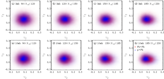
Figure 10: (Color online) The EbyE 2-D distributions of $v_{2}$ vs $v_{3}$ [P($v_{2}$, $v_{3}$)] of Pb$+$Pb (red) and $p$$+$Pb (blue) collisions in the AMPT model with the parton cross section of 3 mb (first row) and 10 mb (second row) for the $N_{ch}$ bin of 90$<N_{ch}<$120 (first column), 120$<N_{ch}<$150 (second column), 150$<N_{ch}<$185 (third column), and 185$<N_{ch}<$230 (fourth column).

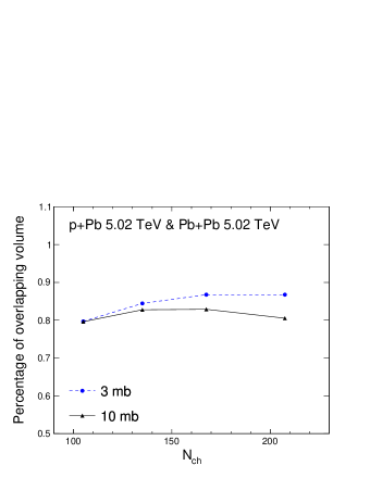
Figure 11: (Color online) The percentage of the 2-D overlapping area between the distribution P($v_{2}$) and P($v_{3}$) for Pb$+$Pb collisions and that for $p$$+$Pb collisions as a function of the number of final charged particles $N_{ch}$ in the AMPT model with the parton cross section of 0 mb (solid curve), 3 mb (dashed curve), and 10 mb (dotted curve).

Figure 10 shows the EbyE 2-D distributions of $v_{2}$ vs $v_{3}$ [P($v_{2}$, $v_{3}$)] in Pb$+$Pb collisions and $p$$+$Pb collisions with parton cross sections of 3 and 10 mb for different $N_{ch}$ classes. Based on P($v_{2}$, $v_{3}$), the percentage of the overlapping area of P($v_{2}$, $v_{3}$) between Pb$+$Pb collisions and $p$$+$Pb collisions as a function of the number of final charged particles $N_{ch}$ can be calculated, which is shown in Fig. 11. Note that the result for 0 mb parton cross section is not shown, since $v_{n}$ come from non-flow for this case. We can see that the overlapping percentage decreases with parton cross section, which indicates that $v_{2}$ and $v_{3}$ between two systems are more different with a larger parton cross section. This is also consistent with the result of validation accuracy in Fig. 7. It suggests that more pronounced difference of collective flow between the two colliding systems is produced by more parton collisions. On the other hand, the large overlapping volume percentage (over $80\%$) indicates that the P($v_{2}$, $v_{3}$) distributions between the two systems are so similar that they are hard to be identified. This is also in line with the observation that PCN can not distinguish the two colliding systems very well in EbyE manner, when we train PCN with input to be the normalized two-momentum of final particles, as shown in Fig. 7.

V Summary and outlook

In summary, we employ the point cloud network to identify the events of $p$$+$Pb and peripheral Pb$+$Pb collisions from a multiphase transport model. Many different features between the two systems are learned and captured by the point cloud network, such as pseudorapidity distribution, $p_{\rm T}$ spectra, anisotropic flow. In the transverse momentum plane, the point cloud network can learn the different features of $p_{\rm T}$ spectra that can classify two different colliding systems. After normalizing transverse momentum of final hadrons, the point cloud network finally distinguish two different colliding systems according to their collective flow. It is difficult for the PCN to distinguish two systems by EbyE collective flow only, since the EbyE distributions of collective flow P($v_{2}$, $v_{3}$) are very close between $p$$+$Pb and Pb$+$Pb collisions. However, the PCN is able to distinguish between two ensembles of each system though the feature of $v_{2}$ and $v_{3}$, and obtain the $N_{ch}$ and parton cross section dependence of the discrepancy between two systems.

In this big data and ML approach, by changing the different input types, we confirm that the discrepancy between two systems is more reflected in the pseudorapidity distribution and the $p_{\rm T}$ spectra than in the anisotropic flow. We also demonstrate that the collective flow between $p$$+$Pb and Pb$+$Pb collisions are more different with a larger parton scattering cross section, which is the consistent with the characteristics of escape mechanism for collective flow in transport model He et al. (2016); Lin et al. (2016).

Admittedly, the ability of our PCN to distinguish $p$$+$Pb from peripheral Pb$+$Pb collisions in EbyE manner by collective flow is limited. However, some meaningful results have been obtained by using the useful tool of machine learning. In future, the method in this study could be applied to investigate other rich physics topics, such as identifying initial flow and final flow in small colliding systems Nie et al. (2019).