Characterizing Long-Tail Categories on Graphs

Abstract.

Long-tail data distributions are prevalent in many real-world networks, including financial transaction networks, e-commerce networks, and collaboration networks. Despite the success of recent developments, the existing works mainly focus on debiasing the machine learning models via graph augmentation or objective reweighting. However, there is limited literature that provides a theoretical tool to characterize the behaviors of long-tail categories on graphs and understand the generalization performance in real scenarios. To bridge this gap, we propose the first generalization bound for long-tail classification on graphs by formulating the problem in the fashion of multi-task learning, i.e., each task corresponds to the prediction of one particular category. Our theoretical results show that the generalization performance of long-tail classification is dominated by the range of losses across all tasks and the total number of tasks. Building upon the theoretical findings, we propose a novel generic framework Tail2Learn to improve the performance of long-tail categories on graphs. In particular, we start with a hierarchical task grouping module that allows label-limited classes to benefit from the relevant information shared by other classes; then, we further design a balanced contrastive learning module to balance the gradient contributions of head and tail classes. Finally, extensive experiments on various real-world datasets demonstrate the effectiveness of Tail2Learn in capturing long-tail categories on graphs.

1. Introduction

The graph provides a fundamental data structure for modeling a wide range of relational data, ranging from financial transaction networks (Wang et al., 2019b; Dou et al., 2020) to e-commerce networks (Wang et al., 2019a; Wu et al., 2021b), from social science (Zhang and Tong, 2016; Fan et al., 2019) to neuroscience (Bessadok et al., 2022; Choi et al., 2017). Graph Neural Networks (GNNs) have achieved outstanding performance on node classification tasks (Zhang et al., 2019; Abu-El-Haija et al., 2020) because of their ability to learn expressive representations from graph-structured data. Despite the remarkable success, the performance of GNNs is mostly attributed to the high-quality and abundant annotated data (Yang et al., 2020; Garcia and Bruna, 2017; Hu et al., 2019; Kim et al., 2019).

Nevertheless, unlike benchmark datasets in ideal scenarios, it is often the case that many high-stake domains naturally exhibit a long-tail distribution, i.e., a few head classes (the majority classes) are well-studied with rich data, while the massive tail classes (the minority classes) are under-explored with scarce data. For example, in financial transaction networks, a few head classes correspond to the normal transaction types (e.g., credit card payment, wire transfer), and the numerous tail classes can represent a variety of fraudulent transaction types (e.g., money laundering, synthetic identity transaction). Despite the rare occurrences of fraudulent transactions, detecting them can prove crucial (Singleton and Singleton, 2010; Akoglu et al., 2015). Another example is the collaboration network. As shown in Figure 1, the Cora-Full network (Bojchevski and Günnemann, 2018) is composed of 70 categories based on research areas, which follow a highly-imbalanced data distribution (e.g., 15 papers in the most niche area while 928 papers in the most popular area). The complex data and task complexity (data imbalance, massive classes) coupled with limited supervision bring enormous challenges to GNNs.

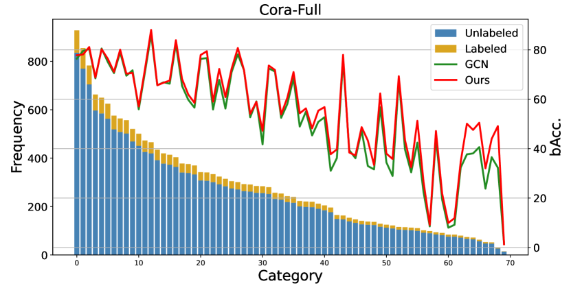
Figure 1. An illustrative figure of long-tail distribution in the collaboration network (Cora-Full (Bojchevski and Günnemann, 2018)), where the green and red curves show balanced accuracy (bAcc) (%) of GCN and Tail2Learn for node classification on each category. Blue and yellow bars represent the class frequency of unlabeled and labeled nodes.

results per class

Important as it could be, there is limited literature that provides a theoretical grounding to characterize the behaviors of long-tail categories on graphs and understand the generalization performance in real environments. To bridge the gap, we provide insights and identify three fundamental challenges in the context of long-tail classification on graphs. First (C1. Highly-skewed data distribution), the data exhibits extremely skewed class memberships. Consequently, the head classes contribute more to the learning objective and can be better characterized by GNNs; the tail classes contribute less to the objective and thus suffer from higher systematic errors(Zhang et al., 2021a). Second (C2. Label scarcity), due to the rarity and diversity of tail classes in nature, it is often more expensive and time-consuming to annotate tail classes rather than head classes (Pelleg and Moore, 2004). What is worse, training GNNs from scarce labels may result in representation disparity and inevitable errors(Zhou et al., 2019; Wang et al., 2021), which amplifies the difficulty of debiasing GNN from the highly-skewed data distribution. Third (C3. Task complexity), with the increasing number of categories, the difficulty of characterizing the support region (Hearst et al., 1998) of categories is dramatically increasing. There is a high risk of encountering overlapped support regions between classes with low prediction confidence (Zhang and Zhou, 2013; Mittal et al., 2021). To deal with the long-tail categories, the existing literature mainly focuses on augmenting the observed graph (Zhao et al., 2021; Wu et al., 2021a; Qu et al., 2021) or reweighting the category-wise loss functions (Yun et al., 2022; Shi et al., 2020). Despite the existing achievements, a natural research question is that: can we further improve the overall performance by learning more knowledge from both head classes and tail classes?

To answer the aforementioned question, we provide the first study on the generalization bound of long-tail classification. The key idea is to formulate the long-tail classification problem in the fashion of multi-task learning (Song et al., 2022), i.e., each task corresponds to the prediction of one particular category. In particular, the generalization bound is in terms of the range of losses across all tasks and the total number of tasks. Building upon the theoretical findings, we propose Tail2Learn, a generic learning framework to characterize long-tail categories on graphs. Specifically, we utilize a hierarchical structure for task grouping to address C2 and C3, which allows the classes with limited labels to benefit from the relevant information shared by other classes. Furthermore, we implement a balanced contrastive module to address C1, which effectively balances the gradient contributions across head classes and tail classes.

In general, our contributions are summarized as follows.

• 1

Problem Definition: We formalize the long-tail classification problem on graphs and develop a novel metric named long-tailedness ratio for characterizing properties of long-tail distributed data.

• 2

Theory: We derive the first generalization bound for long-tail classification on graphs, which inspires our proposed framework.

• 3

Algorithm: We propose a novel approach named Tail2Learn that (1) extracts shareable information across classes via hierarchical task grouping and (2) balances the gradient contributions of head classes and tail classes.

• 4

Evaluation: We identify six real-world datasets for long-tail classification on graphs. We systematically evaluate the performance of Tail2Learn by comparing them with ten baseline models. The results demonstrate the effectiveness of Tail2Learn and verify our theoretical findings.

• 5

Reproducibility: We publish our data and code at https://anonymous.4open.science/r/Tail2Learn-CE08/.

The rest of our paper is organized as follows. In Section 2, we introduce the preliminary and problem definition. In Section 3, we derive the generalization bound of long-tail classification on graphs and present the details of our proposed framework Tail2Learn. Experimental results with discussion are reported in Section 4. In Section 5, we review the existing related literature. Finally, we conclude this paper in Section 6.

2. Preliminary

In this section, we introduce the background and give the formal problem definition. Table 4 in Appendix A summarizes the main notations used in this paper. We use regular letters to denote scalars (e.g. $\mu$), boldface lowercase letters to denote vectors (e.g. $\mathbf{v}$), and boldface uppercase letters to denote matrices (e.g. $\mathbf{X}$).

We represent a graph as $\mathcal{G}=(\mathcal{V},\mathcal{E},\mathbf{X})$, where $\mathcal{V}=\{\mathbf{v}_{1},\ldots,\mathbf{v}_{n}\}$ represent the set of nodes, $n$ is the number of nodes, $\mathcal{E}\subseteq\mathcal{V}\times\mathcal{V}$ represent the set of edges, $\mathbf{X}\in\mathbb{R}^{n\times d}$ represent the node feature matrix, and $d$ is the feature dimension. $\mathbf{A}\in\{0,1\}^{n\times n}$ is the adjacency matrix, where $\mathbf{A}_{ij}=1$ if there is an edge $\mathbf{e}_{ij}\in\mathcal{E}$ from $\mathbf{v}_{i}$ to $\mathbf{v}_{j}$ in $\mathcal{G}$ and $\mathbf{A}_{ij}=0$ otherwise. Next, we briefly review graph neural networks and long-tail classification.

Graph Neural Networks. Graph neural network aims to generate low-dimensional representations in the embedding space that captures graph features and structure. In general, a Graph Convolutional Network (GCN) (Kipf and Welling, 2016) layer can be written as

(1) $$\mathbf{Z}=\sigma\left(\hat{\mathbf{D}}^{-1/2}\hat{\mathbf{A}}\hat{\mathbf{D}}^{-1/2}\mathbf{X}\mathbf{W}\right)$$

where $\sigma$ represents an arbitrary activation function, $\mathbf{W}$ is the weight parameters, $\hat{\mathbf{A}}=\mathbf{A}+\mathbf{I}$ is the augmented adjacency matrix, $\hat{\mathbf{D}}$ is the degree matrix, and $\mathbf{Z}$ is the node embeddings. In this paper, we focus on node classification task, it encompasses training a GNN to predict labels of nodes and learn a mapping function $f:\mathcal{V}\rightarrow\mathcal{Y}$.

Long-Tail Classification. Long-tail classification refers to the classification problem in the presence of a massive number of classes and highly-skewed class-membership distribution, where head classes have abundant instances, while the tail classes have few or even only one instance. Here $\mathcal{D}=\{(\mathbf{x}_{i},y_{i})\}_{i=1}^{n}$ represents a dataset with long-tail distribution, $T$ is the number of classes in $\mathcal{D}$, and $\mathcal{D}_{t}$ represents the set of instances belonging to class $t$. Without the loss of generality, we define the long-tail dataset as a dataset $\mathcal{D}=\{\mathcal{D}_{1},\mathcal{D}_{2},\ldots,\mathcal{D}_{T}\}$, where $|\mathcal{D}_{1}|\geq|\mathcal{D}_{2}|\geq\cdots\gg|\mathcal{D}_{T}|$ and $\sum_{t=1}^{T}|\mathcal{D}_{t}|=n$. To measure the skewness of long-tail distribution, (Wu et al., 2021a) introduces the Class-Imbalance Ratio as $\frac{\min_{t}(|\mathcal{D}_{t}|)}{\max_{t}(|\mathcal{D}_{t}|)}$, that is the ratio of the size of the largest majority class to the size of the smallest minority class.

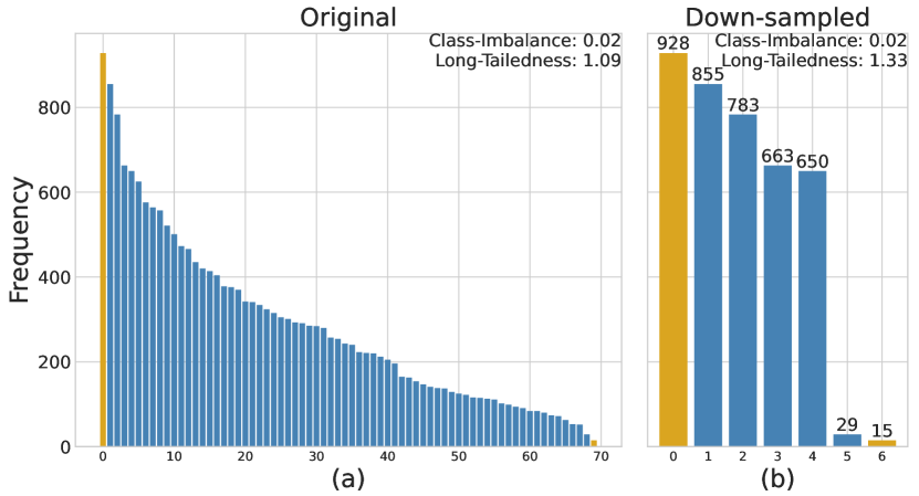
Figure 2. Comparison between two long-tail distribution metrics on (a) the hard case of the original Cora-Full dataset and (b) the easy case of the down-sampled Cora-Full dataset. We observe that the class-imbalance ratio falls short in characterizing the task complexity of two datasets, while the long-tailedness ratio does.

ratioExample

Problem Definition. We consider a graph $\mathcal{G}$ with long-tail distribution. While Class-Imbalance Ratio in (Wu et al., 2021a) considers the imbalanced data distribution but overlooks the task complexity in the task of long-tail classification. As the number of categories increases, the difficulty of the classification task therefore increases. For example, we down-sampled 7 categories from the original Cora-Full dataset, as shown in Figure 2. Although the class-imbalance ratio remains the same (0.02 for both the original and down-sampled datasets), the task complexity varies significantly, i.e., 70 classes in Figure 2 (a) v.s 7 classes in Figure 2 (b). For this reason, we introduce a novel quantile-based metric named long-tailedness ratio to jointly quantify the class-imbalance ratio and task complexity for the long-tail datasets. It is notable that the proposed metric is general and not limited to graph-structured data. The formal definition of long-tailedness ratio is provided as follows:

Definition 0 (Long-Tailedness Ratio).

Suppose we have a dataset $\mathcal{D}$ with long-tail categories that follows a descending order in terms of the number of instances. The long-tailedness ratio is defined as

$$\texttt{Ratio}_{LT}(p)=\frac{Q(p)}{T-Q(p)}$$

where $Q(p)=min\{y:Pr(\mathcal{Y}\leq y)=p,1\leq y\leq T\}$ is the quantile function of order $p\in(0,1)$ for variable $\mathcal{Y}$, $T$ is the number of categories. The numerator represents the number of categories to which $p$ percent instances belongs, and the denominator represents the number of categories to which the else $(1-p)$ percent instances belongs in $\mathcal{D}$.

Essentially, the long-tailedness ratio implies the task complexity of long-tail classification and characterizes two properties of $\mathcal{D}$: (1) class-membership skewness, (2) # of classes. Intuitively, the higher the skewness of the data distribution, the lower the ratio will be; the higher the complexity of the tasks (i.e., massive number of classes), the lower the long-tailedness ratio. Figure 2 provides a case study on Cora-Full dataset by comparing long-tailedness ratio and class-imbalance ratio (Wu et al., 2021a) introduced previously. In general, we observe that unlike the class-imbalance ratio, long-tailedness ratio better characterizes the differences on the original Cora dataset ($\texttt{Ratio}_{LT}(0.8)=1.09$) and its down-sampled dataset ($\texttt{Ratio}_{LT}(0.8)=1.33$). In our implementation, we choose $p=0.8$ following the Pareto principle (Pareto et al., 1971).

As shown in Figure 1, there are several obstacles to long-tail classification. First of all, highly skewed data make graph models biased toward head classes and do not perform well on tail classes. Moreover, the training for tail-class classification suffers from the lack of labeled instances in tail classes. Last but not least, these methods fail to consider the complexity of the long-tail distribution, i.e., when the number of categories increases, a large number of tail classes are encountered, which exacerbates the complexity of the task. Most previous work (Park et al., 2022; Zhao et al., 2021; Wu et al., 2021a; Qu et al., 2021; Liu et al., 2021) about long-tail classification on graphs focus on designing different augmentation and/or reweighting methods to address this issue, while lack of theoretical analysis. Given the notations above, we formally define the problem as follows.

Problem 1.

Graph-based Long-Tail Category Characterization
Given: (i) an input graph $\mathcal{G}=(\mathcal{V},\mathcal{E},\mathbf{X})$ with low long-tailedness ratio $\texttt{Ratio}_{LT}$, (ii) few-shot annotated data $\mathcal{Y}$ for each class.
Find: Accurate predictions $\hat{\mathcal{Y}}$ of unlabeled nodes across both head and tail classes in the graph $\mathcal{G}$.

3. Tail2Learn Model

In this section, we introduce a generic learning framework named Tail2Learn, which aims to characterize long-tail categories on graphs and improve the model’s performance on tail-class nodes. For the first time, we propose to reformulate the long-tail classification problem in the manner of multi-task learning. We derive a generalization bound (Sec 3.1), which implies the performance of long-tail classification is dominated by two factors: the number of tasks and the range of losses across all tasks. The former item inspires us to construct a hierarchical task grouping module (Sec 3.2), which enables information sharing across different tasks. The latter item leads us to develop a balanced contrastive learning module (Sec 3.2) for balancing the contribution of head class nodes and tail class nodes to the overall objective function. Finally, we present an end-to-end optimization algorithm for Tail2Learn (Sec 3.3).

3.1. Theoretical Analysis

In this subsection, we propose the very first generalization guarantee under the setting of long-tail categories on graphs. In this paper, we consider the classification for each category as a learning task on graph $\mathcal{G}$, $\mathbf{X}$ is the node features, $\mathcal{Y}$ is the labels, and there are $T$ tasks and $n$ nodes overall. The training set for the $t^{\text{th}}$ task $\mathcal{D}_{t}=\{(\mathbf{x}^{t}_{i},y^{t}_{i})\}_{i=1}^{n_{t}}$ contains $n_{t}$ annotated nodes, $\mathbf{x}^{t}_{i}$ is the $i^{\text{th}}$ training node in class $t$, and $y^{t}_{i}=t$ for all $i$. Note that different tasks are contained in the same feature space, thus we have $\mathbf{x}^{t}_{i}\in\mathbb{R}^{d},\forall t,i$. $\mathbf{X}_{t}$ represents the $d$-dimensional feature matrix of all node in class $t$ and follows probability measure $\mu_{t}$, i.e., $\{\mathbf{X}_{1},\ldots,\mathbf{X}_{T}\}\sim\prod_{t=1}^{T}\left(\mu_{t}\right)^{n_{t}}$.

A key assumption of our work is task relatedness, i.e., relevant tasks should share similar model parameters. Thus, jointly learning relevant tasks together can potentially improve both tasks. Our goal is to learn these tasks concurrently to enhance the overall performance of each task. The hypothesis $g$ of multi-task learning model can be represented by $g=\{f_{t}\}_{t=1}^{T}\circ h$, where $\circ$ is the functional composition, $g_{t}(x)=f_{t}\circ h(x)\equiv f_{t}(h(x))$ for each classification task. The function $h:\mathbf{X}\rightarrow\mathbb{R}^{K}$ is the representation extraction function shared across different tasks, $f:\mathbb{R}^{K}\rightarrow\mathbb{R}$ is the task-specific predictor, and $K$ is the dimension of hidden layer. The task-averaged risk of representation $h$ and predictors $f_{1},\ldots,f_{T}$ is defined as $\epsilon\left(h,f_{1},\ldots,f_{T}\right)$, and the corresponding empirical risk is defined as $\hat{\epsilon}\left(h,f_{1},\ldots,f_{T}\right)$.

(2) $$\epsilon\left(h,f_{1},\ldots,f_{T}\right)=\frac{1}{T}\sum_{t=1}^{T}\mathbb{E}_{(\mathbf{X},\mathcal{Y})\sim\mu_{t}}l\left(f_{t}(h(\mathbf{X})),\mathcal{Y}\right)$$

(3) $$\hat{\epsilon}\left(h,f_{1},\ldots,f_{T}\right)=\frac{1}{T}\sum_{t=1}^{T}\frac{1}{n_{t}}\sum_{i=1}^{n_{t}}l\left(f_{t}(h(\mathbf{X})),\mathcal{Y}\right)$$

where $l(\cdot,\cdot)$ is a loss function. To drive the generalization error for long-tail classification on graphs with respect to $\epsilon\left(h,f_{1},\ldots,f_{T}\right)$ and $\hat{\epsilon}\left(h,f_{1},\ldots,f_{T}\right)$, we formally define the loss range of $f_{1},\ldots,f_{T}$ in Definition 1:

Definition 0 (Loss Range).

In multi-task learning, the loss range of the $T$ predictors $f_{1},\ldots,f_{T}$ is defined as the difference between the lowest and highest values of the loss function across all tasks.

(4) $$\texttt{Range}(f_{1},\ldots,f_{T}) =\max_{t}\frac{1}{n_{t}}\sum_{i=1}^{n_{t}}l(f_{t}(h(\mathbf{x}^{t}_{i})),y^{t}_{i})$$

$$-\min_{t}\frac{1}{n_{t}}\sum_{i=1}^{n_{t}}l(f_{t}(h(\mathbf{x}^{t}_{i})),y^{t}_{i})$$

where $l(\cdot,\cdot)$ is a loss function. For the case of the node classification, $l(\cdot,\cdot)$ refers to cross-entropy loss.

In the scenario of long-tail class-membership distribution, there often exists a tension between maintaining head class performance and improving tail class performance (Zhang et al., 2021a). Minimizing the losses of the head classes may lead to a biased model, which increases the losses of the tail classes. Under the premise that the model could keep a good performance on head tasks, controlling the loss range could improve the performance on tail tasks and lead to a better generalization performance of the model. Here, we drive the range-based generalization error bound for long-tail categories in the following three steps: (S1) giving the loss-related generalization error bound based on the Gaussian complexity-based bound; (S2) giving the hypothesis $g$-related generalization error bound based on the loss-related error bound in S1 and the property of Gaussian complexity; (S3) deriving the generalization error bound related to representation extraction $h$ and the range of task-specific predictors $f_{1},\ldots,f_{T}$ based on the obtained hypothesis $g$-related bound in S2. Based on (Maurer et al., 2016), we can derive the Gaussian complexity-based bound on the training set $\mathbf{X}$ as follows.

Lemma 0 (Gaussian Complexity-Based Bound).

Let $\mathcal{F}$ be a class of functions $f:\mathbf{X}\rightarrow[0,1]^{T}$, and $\mathbf{x}^{t}_{i}$ represents $i^{\text{th}}$ instances belonging to class $t$. Then, with probability greater than $1-\delta$ and for all $f\in\mathcal{F}$, we have

(5) $$\frac{1}{T}\sum_{t}\left(\mathbb{E}_{\mathbf{X}\sim\mu_{t}}\left[f_{t}(\mathbf{X})\right]-\sum_{i}\frac{1}{n_{t}}f_{t}\left(\mathbf{x}^{t}_{i}\right)\right)$$

$$\leq \sum_{t}\left(\frac{\sqrt{2\pi}G(\mathcal{Y})}{n_{t}}+\sqrt{\frac{9\ln(2/\delta)}{2n_{t}}}\right)$$

where $\mu_{1},\ldots,\mu_{T}$ are probability measures, $\mathcal{Y}\subset\mathbb{R}^{n}$ is the random set obtained by $\mathcal{Y}=\left\{\left(f_{t}\left(\mathbf{x}^{t}_{i}\right)\right):f_{t}\in\mathcal{F}\right\}$, and $G$ is Gaussian complexity.

Lemma 2 yields that the task-averaged estimation error is bounded by the Gaussian complexity in multi-task learning. Based on the key property of the Gaussian averages of a Lipschitz image given in Lemma 3, we can move to the second step and derive the hypothesis $g$-related generalization error bound for long-tail on graphs.

Lemma 0 (Property of Gaussian Complexity (Maurer et al., 2016)).

Suppose $\mathcal{Y}\subseteq\mathbb{R}^{n}$ and $\phi:\mathcal{Y}\rightarrow\mathbb{R}^{m}$ is (Euclidean) Lipschitz continuous with Lipschitz constant $L$, we have

(6) $$G(\phi(\mathcal{Y}))\leq LG(\mathcal{Y})$$

From Lemma 3, we obtain the hypothesis $g$-related bound in Eq. (19). Next, we move to the third step: derived the generalization bound related to $h$ and $f_{1},\ldots,f_{T}$, according to the chain rule of gaussian complexity presented in Lemma 4.

Lemma 0 (Chain Rule of Gaussian Complexity).

Suppose we have $\mathcal{Y}\subseteq\mathbb{R}^{n}$ with (Euclidean) diameter $D(\mathcal{Y})$. $\mathcal{F}$ is a class of functions $f:\mathcal{Y}\rightarrow\mathbb{R}^{m}$, all of which have Lipschitz constant at most $L(\mathcal{F})$. Then, for any $y_{0}\in\mathcal{Y}$,

$$G(\mathcal{F}(\mathcal{Y}))\leq c_{1}L(\mathcal{F})G(\mathcal{Y})+c_{2}D(\mathcal{Y})\texttt{Range}(f_{1},\ldots,f_{T})+G\left(\mathcal{F}\left(y_{0}\right)\right),$$

where $c_{1}$ and $c_{2}$ are universal constants.

Finally, the generalization error bound under the setting of long-tail categories on graphs is given as in the following Theorem 5.

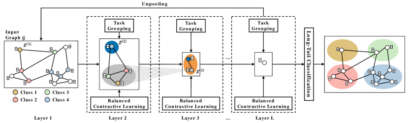
Figure 3. The proposed Tail2Learn framework with $L$ task-grouping layers.

framework

Theorem 5 (Generalization Error Bound).

Given the representation extraction function $h\in\mathcal{H}$ and the task-specific predictor $f_{1},\ldots,f_{T}\in\mathcal{F}$, with probability at least $1-\delta,\delta\in[0,1]$, in the draw of a multi sample $\prod^{T}_{t=1}\mu_{t}^{n_{t}}$, we have

(7) $$\mathcal{E}-\hat{\mathcal{E}}\leq \sum_{t}\left(\frac{c_{1}LG(\mathcal{H}(\mathbf{X}))}{n_{t}}+\frac{c_{2}\sup_{h\in\mathcal{H}}\|h(\mathbf{X})\|\texttt{Range}(f_{1},\ldots,f_{T})}{n_{t}}\right.$$

$$+ \left.\sqrt{\frac{9\ln(2/\delta)}{2n_{t}}}\right)$$

where $\mathbf{X}$ is the node feature, $T$ is the number of tasks, $n_{t}$ is the number of nodes in task $t$, $c_{1}$ and $c_{2}$ are universal constants.

The proofs of Lemma 2, Lemma 4, and Theorem 5 are provided in Appendix B. Theorem 5 implies that the generalization error bound is upper bounded by the Gaussian complexity of the shared representation extraction $h$, the loss range of the task-specific predictors $f_{1},\ldots,f_{T}$, the number of total tasks and the sum of their reciprocal. Regularizing the number of tasks $T$ and the loss range $\texttt{Range}(f_{1},\ldots,f_{T})$ can tighten this upper bound, which motivates the development of Tail2Learn in the following subsection.

3.2. Tail2Learn Framework

The overview of Tail2Learn is presented in Figure 3, which consists of two major modules: M1. hierarchical task grouping and M2. long-tail balanced contrastive learning. Specifically, the theoretical analysis in Theorem 5 inspires that reducing the number of total tasks can improve the generalization ability. Thus, in order to alleviate C2 (Label scarcity) and C3 (Task complexity), M1 is designed to minimize the number of tasks and capture the information shared across tasks to improve overall performance. Another key message from Theorem 1 is that reducing the range of losses across all tasks while ensuring the performance on head tasks can improve the generalization ability. Thus, in M2, we designed a long-tail balanced contrastive loss to balance the head classes and the tail classes and control the loss range. Moreover, M2 is also a natural solution to C1 (High-skewed data distribution) because it reduces the dominance of head classes and emphasizes the importance of tail classes. Overall, both M1 and M2 are mutually beneficial in the task of characterizing long-tail categories on graphs. In particular, M1 ensures accurate prototype embeddings of tasks that could benefit the contrastive learning in M2, while M2 ensures accurate node embeddings by pooling together similar nodes and pushing away dissimilar nodes that could help improve learned node embeddings in M1. Our ablation study (Table 3) firmly attests they both are essential in successfully long-tail classification on graphs.

In the following subsections, we dive into the two modules of Tail2Learn in detail.

M1. Hierarchical Task Grouping. We propose to address C2 (Label scarcity) and C3 (Task complexity) for characterizing long-tail categories on graphs by leveraging the information learned in one category to help train another category. Inspired by multi-task learning, we implement task grouping (Song et al., 2022) to share information across different tasks via hierarchical pooling (Ma et al., 2019; Ranjan et al., 2020; Lee et al., 2019; Ying et al., 2018; Gao and Ji, 2019). The core idea of hierarchical pooling is to choose the important nodes and preserve the original connections between chosen nodes as edges to generate a coarsened graph. As shown in Figure 4, the task grouping operation is composed of two steps: (Step 1) we group nodes into several tasks, and (Step 2) learn the embeddings of the task prototypes. This operation can be easily generalized to the $l^{\text{th}}$ layers, which leads to the hierarchical task grouping.

Specifically, we first generate a low-dimensional node embedding vector for each node $\mathbf{Z}^{(1)}=(\mathbf{z}^{(1)}_{1},\ldots,\mathbf{z}^{(1)}_{n})$ via GCN layers (Eq. (1)). Next, we group nodes into tasks (with the same number of categories), and then group these tasks into hypertasks by stacking several task grouping layers. Following (Gao and Ji, 2019), in the $l^{\text{th}}$ layer, we perform down-sampling on the graph and learn top $T^{(l)}$ nodes. The $l^{\text{th}}$ task grouping layer is defined as:

(8) $$\mathcal{I}=\texttt{TOP-RANK}(\texttt{PROJ}(\mathbf{Z}^{(l)}),T^{(l)})$$

$$\mathbf{X}^{(l+1)}=\mathbf{Z}^{(l)}(\mathcal{I},:)\odot\left(\texttt{PROJ}(\mathbf{Z}^{(l)})\mathbf{1}_{d}^{T}\right)$$

$$\mathbf{A}^{(l+1)}=\mathbf{A}^{(l)}(\mathcal{I},\mathcal{I})$$

where $l=1,\ldots L$, $\texttt{PROJ}(\cdot,\cdot)$ is a differentiable projection to map each embedding $\mathbf{z}^{(l)}$ to a scalar, the function TOP-RANK selects nodes with the largest value after projection. We generate a new graph with the selected $T^{(l)}$ nodes representing the prototypes of tasks, where $T^{(l)}$ represents the number of tasks. $\mathcal{I}$ is the indexes representing the selected nodes and implies a task grouping process. The connectivity between the selected nodes remains as edges of the new graph, and the new adjacency matrix and feature matrix are constructed by row and/or column extraction. $\mathbf{1}_{d}$ represents a $d$-dimensional all-ones vector, and $\odot$ is the element-wise matrix multiplication. The subsequent GCN layer aggregates information from the first-order neighbor of each node based on $\mathbf{X}^{(l+1)}$ and $\mathbf{A}^{(l+1)}$ and then outputs the embeddings $\mathbf{Z}^{(l+1)}$ of the new graph. Notably, $\mathbf{Z}^{(1)}$ is the node embeddings, $\mathbf{Z}^{(2)}$ is the embeddings of the task prototypes corresponding to the categories, and $\mathbf{Z}^{(l)}(l>2)$ is the embeddings of the hypertask prototypes.

The number of tasks $T^{(l)}$ represents the level of abstraction of task grouping, and decreases as the task grouping layer gets deeper. In high level layers ($l>2$), the number of tasks may be smaller than the number of categories. By controlling $T^{(l)}$, information shared across tasks can be obtained to alleviate the task complexity (as the number of categories increases, characterizing them become difficult). Meanwhile, in a deep level of abstraction, nodes that come from different categories with high-level semantic similarities can be assigned to one task. By sharing label information with other different categories within the same hypertask, the problem of label scarcity can be alleviated. As shown in Figure 3, we consider a special case of 2 head classes (i.e., class 2 and 4) and 2 tail classes (i.e., class 1 and 3). By grouping the prototype of class 1, class 2, and class 3 into the same hypertask at layer 3, the labels available for class 1 are extended from $n_{1}$ to $n_{1}+n_{2}+n_{3}$.

In order to well capture the hierarchical structure of tasks and propagate information across different tasks, we need to restore the original resolutions of the graph to perform node classification. Specifically, we stack the same number of unpooling layers as the task grouping layers, which up-samples the features to restore the original resolutions of the graph. To achieve this, the locations of nodes selected in the corresponding task grouping layer are recorded and applied in placing the nodes back to their original positions. The mathematical form of the propagation rule can be expressed as follows:

(9) $$\mathbf{X}^{(l+1)}=\texttt{DIST}\left(0_{n\times d},\mathbf{X}^{(l+1)},\mathcal{I}\right)$$

where $0_{n\times d}$ represents the initially all-zeros feature matrix, $X^{(l+1)}\in\mathbb{R}^{T^{(l)}\times d}$ represents the feature matrix of the current graph, $\mathcal{I}$ represents the indices of selected nodes in the corresponding task grouping layer, and DIST distributes row vectors in $X^{(l+1)}$ into matrix $0_{n\times d}$ based on their corresponding indices $\mathcal{I}$. Finally, the corresponding blocks of the task grouping and unpooling layers are skip-connected by feature addition, and the final node embeddings are passed to an MLP layer for final predictions.

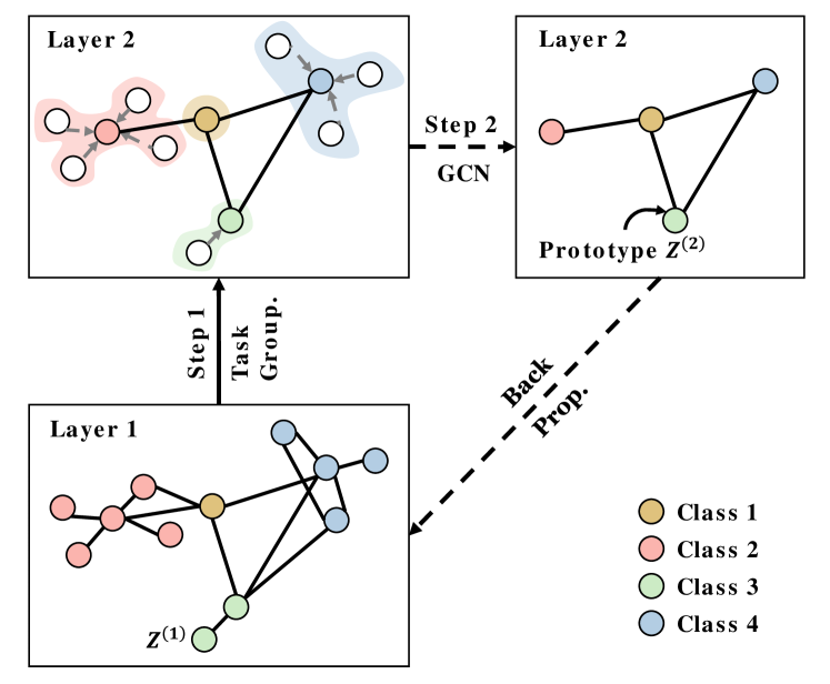
Figure 4. An illustrative figure for M1 with two task-grouping layers. Step 1: nodes are first grouped into four tasks (each representing a class). Step 2: We learn the embeddings of the task prototypes. Finally, the node embeddings are updated by back-propagation.

M1

M2. Long-Tail Balanced Contrastive Learning. To better handle long-tail classification and solve C1 (High-skewed data distribution), we introduce a principled graph contrastive learning algorithm to further regularize M1 (Hierarchical task grouping). Graph contrastive learning (GCL) (Xu et al., 2021; Hassani and Khasahmadi, 2020; Qiu et al., 2020; Zhang et al., 2021b; Zhu et al., 2021) has achieved supreme performance in various tasks with graph-structure data and can be used to mitigate long-tail classification. It aims to learn efficient graph/node representations by constructing positive and negative instance pairs. However, many existing graph contrast learning models are unsupervised, i.e., the label information is not leveraged in training. Therefore, the representation clusters learned by GCL may not correspond to long-tail categories. For example, in Figure 4, class 1 may have very few nodes and is incorrectly merged into class 2 under unsupervised learning at layer 1. This error is fatal for the tail category in the long-tail classification.

In this paper, we propose to incorporate supervision signals into graph contrastive learning. The embeddings for implementing contrastive learning are learned from task grouping with label information, and the prototypes are restricted to be relevant to the categories. By performing contrastive learning, we pull the node embeddings together with their corresponding prototypes and push them away from other prototypes to improve the performance of long-tailed classification. In particular, different from the vanilla InfoNCE (Oord et al., 2018), here we utilize balanced contrastive learning (Zhu et al., 2022) to balance the gradient contribution of different categories. For $l^{\text{th}}$ task grouping layer, we group nodes in layer $l$ into $T^{(l+1)}$ tasks and calculate the balanced contrastive loss based on the node embeddings $\mathbf{Z}^{(l)}$ and the task prototypes $\mathbf{Z}^{(l+1)}$. Here the prototypes of tasks are calculated based on labels and are therefore category-specific. The mathematical form of the loss function $\mathcal{L}_{BCL}$ of M1 can be expressed as follows:

(10) $$\mathcal{L}_{BCL}(\mathbf{z}_{i})=-\frac{1}{n_{t}}\times$$

$$\sum_{j\in\mathcal{V}_{t}\backslash i}\log\frac{\exp\left(\mathbf{z}_{i}\cdot\mathbf{z}_{j}/\tau\right)}{\sum_{1\leq q\leq T}\frac{1}{n_{q}+1}\sum_{k\in\mathcal{V}_{q}}\exp\left(\mathbf{z}_{i}\cdot\mathbf{z}_{k}/\tau\right)}$$

where we suppose $\mathbf{z}_{i}$ belongs to task $t$, here $\mathcal{V}_{t}$ are all the nodes within the $t^{\text{th}}$ task including the prototype $\mathbf{z}^{(l+1)}_{t}$, $n_{t}$ represents the number of nodes in task $t$, $z_{k}=z^{(l)}_{k}$ represents the embedding of the $k^{\text{th}}$ node, temperature $\tau$ controls the strength of penalties on negative nodes, and we assign each node to the nearest task prototype. According to M1, we set the number of tasks $T^{(1)}$ equal to the number of categories $T$ for the first layer.

Therefore, $\mathcal{L}_{BCL}$ solves the long-tail classification in two aspects: (1) $\mathcal{L}_{BCL}$ reduces the proportion of head classes and highlights the importance of tail classes. The $n_{j}+1$ term in the denominator averages over the nodes of each category in order that each category has an approximate contribution for optimizing; (2) the set of $T$ prototypes is added to obtain a more stable optimization for balanced contrastive learning.

In addition, we introduce the supervised contrastive loss on the restored original graph. It makes node pairs belonging to the same category close to each other while pairs not belonging to the same category far apart. Unlike $\mathcal{L}_{BCL}$ which uses task information from task grouping, $\mathcal{L}_{SCL}$ uses label information:

(11) $$\mathcal{L}_{SCL}(\mathbf{z}_{i})=-\frac{1}{n_{t}}\times\sum_{j\in\mathcal{V}_{t}\backslash i}\log\frac{\exp\left(\mathbf{z}_{i}\cdot\mathbf{z}_{j}/\tau\right)}{\sum_{1\leq q\leq T}\frac{1}{n_{q}}\sum_{k\in\mathcal{V}_{q}}\exp\left(\mathbf{z}_{i}\cdot\mathbf{z}_{k}/\tau\right)}$$

where $\mathbf{z}_{i}$ belongs to class $t$, $n_{t}$ represents the number of nodes in class $t$, $z_{k}$ represents the embedding of the $k^{\text{th}}$ node, and $\tau$ is the temperature. In summary, M2 uses balanced contrastive loss and supervised contrastive loss to balance the performance of the head and tail classes to solve the high-skewed data distribution.

Theorem 5 shows that the generalization performance of long-tail categories on graphs can be improved by (1) reducing the loss range across all tasks $\texttt{Range}(f_{1},\ldots,f_{T})$, as well as (2) controlling the total number of tasks $T$. Below we give a corollary to theoretically explain how the two modules in Tail2Learn works.

Corollary 0 (Effectiveness of Tail2Learn).

Consider a long-tail classification with node feature matrix $\mathbf{X}$, and the total number of instances is $n$. For the $l^{\text{th}}$ layer of Tail2Learn, we group nodes into $T^{(l)}$ tasks, and the task-specific predictors are $f_{1}^{(l)},\ldots,f_{T}^{(l)}$. For the $(l+1)^{\text{th}}$ layer, we group nodes into $T^{(l+1)}$ tasks with $T^{(l+1)}<T^{(l)}$. In addition, we can learn the task-specific predictors $f_{1}^{(l+1)},\ldots,f_{T}^{(l+1)}$ with $\texttt{Range}(f_{1}^{(l+1)},\ldots,f_{T}^{(l+1)})<\texttt{Range}(f_{1}^{(l)},\ldots,f_{T}^{(l)})$. Then we have that the upper bound of the error for $(l+1)^{\text{th}}$ layer is smaller than the upper bound for $l^{\text{th}}$ layer given in Tail2Learn  i.e.,

(12) $$\sum_{t}\left(\frac{c_{1}LG(\mathcal{H}(\mathbf{X}))}{n_{t}^{(l+1)}}+\frac{c_{2}\sup_{h\in\mathcal{H}}\|h(\mathbf{X})\|\texttt{Range}(f_{1}^{(l+1)},\ldots,f_{T}^{(l+1)})}{n_{t}^{(l+1)}}\right.$$

$$\left.+\sqrt{\frac{9\ln(2/\delta)}{2n_{t}^{(l+1)}}}\right)\leq\sum_{t}\left(\frac{c_{1}LG(\mathcal{H}(\mathbf{X}))}{n_{t}^{(l)}}\right.$$

$$\left.+\frac{c_{2}\sup_{h\in\mathcal{H}}\|h(\mathbf{X})\|\texttt{Range}(f_{1}^{(l)},\ldots,f_{T}^{(l)})}{n_{t}^{(l)}}+\sqrt{\frac{9\ln(2/\delta)}{2n_{t}^{(l)}}}\right)$$

where the shared representation extraction is $h\in\mathcal{H}$. The number of instances in the $t^{\text{th}}$ class for layer $l$ is $n^{(l)}_{t}$, and the number of instances in the $t^{\text{th}}$ class for layer $(l+1)$ is $n^{(l+1)}_{t}$, $\sum_{t}n^{(l)}_{t}=\sum_{t}n^{(l+1)}_{t}=n$.

Proof.

The proof is provided in Appendix B. ∎

Remark: Corollary 6 theoretically demonstrate the effectiveness of Tail2Learn. Our algorithm leads to a significantly improved generalization error bound in long-tail classification on graph, by reducing the number of tasks in M1 and controlling the loss range $\texttt{Range}(f_{1},\ldots,f_{T})$ in M2.

3.3. Optimization

Overall, the goal of the training process is to minimize the node classification loss (for few-shot annotated data), the unsupervised balanced contrastive loss (for task combiations in each layer), and the supervised contrastive loss (for categories). The node classification loss is defined as follows:

(13) $$\mathcal{L}_{NC}=\sum_{i=1}^{T}\mathcal{L}_{CE}\left(g(\mathcal{G}),\mathcal{Y}\right)$$

where $\mathcal{L}_{CE}$ is the cross-entropy loss, $\mathcal{G}$ represents the input graph with few-shot labeled nodes and $\mathcal{Y}$ represents the labels. Then the overall loss function can be written as follows:

(14) $$\mathcal{L}_{total}=\mathcal{L}_{NC}+\gamma*(\mathcal{L}_{BCL}+\mathcal{L}_{SCL})$$

where $\gamma$ balances the contribution of the three terms.

The pseudo-code of Tail2Learn is provided in Algorithm 1 in Appendix C. Given an input graph $\mathcal{G}$ with few-shot label information $\mathcal{Y}$, our proposed Tail2Learn framework aims to predict $\hat{\mathcal{Y}}$ of unlabeled nodes in graph $\mathcal{G}$. We initialize all the task grouping, the unpooling layers and the classifier in Step 1. Steps 4-6 correspond to the task grouping process: We generate down-sampling graphs and compute node representations using GCNs. Then Steps 7-9 correspond to the unpooling process: We restore the original graph resolutions and compute node representations using GCNs. An MLP is followed for computing predictions after skip-connections between the task grouping and unpooling layers in Step 10. Finally, in Step 11, models are trained by minimizing the objective function. In Steps 13, we return predicted labels $\hat{\mathcal{Y}}$ in the graph $\mathcal{G}$ based on the trained classifier.

4. Experiments

In this section, we evaluate the effectiveness of Tail2Learn on six benchmark datasets. Tail2Learn exhibits superior performances compared to several state-of-the-art baselines. We demonstrate the necessity of each component of Tail2Learn in ablation studies. We also report the parameter and complexity sensitivity of Tail2Learn in Appendix G, which shows that Tail2Learn achieves a convincing performance with minimal tuning efforts and is scalable.

4.1. Experiment Setup

Datasets: We evaluate our proposed framework on Cora-Full (Bojchevski and Günnemann, 2018), BlogCatalog (Tang and Liu, 2009), Email (Yin et al., 2017), Wiki (Mernyei and Cangea, 2020), Amazon-Clothing (McAuley et al., 2015), and Amazon-Electronics (McAuley et al., 2015) datasets to perform node classification. The first four datasets naturally have a smaller long-tailedness ratio, indicating that they are more long-tailed; while the last two datasets have a larger long-tailedness ratio, so we manually process them to make the long-tailedness ratio of order 0.8 ($\texttt{Ratio}_{LT}(0.8)$) of train sets approximately equal to 0.25. Further details, additional processing, and statistics (including class-imbalance ratio and long-tailedness ratio) of the six datasets are in Appendix D.

Comparison Baselines: We compare Tail2Learn with the following five imbalanced classification methods and five GNN-based long-tail classification methods. The details of baselines are further described in Appendix E.

• 1

Imbalanced classification methods: Origin (i.e., GCN (Kipf and Welling, 2017)), Over-sampling (Chawla, 2003), Re-weighting (Yuan and Ma, 2012), SMOTE (Chawla et al., 2002), and Embed-SMOTE (Ando and Huang, 2017) are five classical imbalance classification models.

• 2

GNN-based long-tail classification methods: Two popular variants of GraphSMOTE (Zhao et al., 2021) ($\text{GraphSMOTE}_{T}$ and $\text{GraphSMOTE}_{O}$), GraphMixup (Wu et al., 2021a), ImGAGN (Qu et al., 2021), and LTE4G (Yun et al., 2022) are five state-of-the-art GNN-based long-tail classification models.

Implementation Details: For evaluations of Tail2Learn, we perform node classification under highly long-tail distribution, with Adam (Kingma and Ba, 2015) as the optimizer. We run all the experiments with 10 different random seeds and report the evaluation metrics along with standard deviations. The parameter settings are included in Appendix F.

Considering the long-tail class-membership distribution, balanced accuracy (bAcc), Macro-F1 and Geometric Means (G-Means) are used as the evaluation metrics, and accuracy (Acc) is also reported as the traditional evaluation metric. Notably, for Amazon-Clothing and Amazon-Electronics, we keep the same number of nodes for each category as test instances, so the values of bAcc and Acc are the same.

4.2. Performance Analysis

	Method	Amazon-Clothing				Amazon-Electronics
		bAcc.	Macro-F1	G-Means	Acc.	bAcc.	Macro-F1	G-Means	Acc.
Classical	Origin	$9.9\pm 0.2$	$9.5\pm 0.2$	$31.3\pm 0.3$	$9.9\pm 0.2$	$16.9\pm 0.2$	$15.2\pm 0.2$	$41.0\pm 0.3$	$16.9\pm 0.2$
	Over-sampling	$9.9\pm 0.2$	$9.5\pm 0.2$	$31.3\pm 0.3$	$9.9\pm 0.2$	$16.8\pm 0.1$	$15.1\pm 0.1$	$40.9\pm 0.2$	$16.8\pm 0.1$
	Re-weight	$10.0\pm 0.2$	$9.6\pm 0.2$	$31.4\pm 0.3$	$10.0\pm 0.2$	$17.0\pm 0.2$	$15.2\pm 0.2$	$41.1\pm 0.3$	$17.0\pm 0.2$
	SMOTE	$10.0\pm 0.1$	$9.5\pm 0.2$	$31.4\pm 0.2$	$10.0\pm 0.1$	$16.9\pm 0.2$	$15.1\pm 0.2$	$41.0\pm 0.3$	$16.9\pm 0.2$
	Embed-SMOTE	$9.9\pm 0.2$	$9.5\pm 0.2$	$31.3\pm 0.3$	$9.9\pm 0.2$	$17.0\pm 0.2$	$15.2\pm 0.2$	$41.1\pm 0.3$	$17.0\pm 0.2$
GNN-based	$\text{GraphSMOTE}_{T}$	$11.7\pm 0.2$	$10.4\pm 0.3$	$34.0\pm 0.3$	$11.7\pm 0.2$	$18.2\pm 0.2$	$15.6\pm 0.2$	$42.5\pm 0.2$	$18.2\pm 0.2$
	$\text{GraphSMOTE}_{O}$	$11.7\pm 0.2$	$10.4\pm 0.3$	$34.0\pm 0.3$	$11.7\pm 0.2$	$18.2\pm 0.2$	$15.5\pm 0.2$	$42.5\pm 0.2$	$18.2\pm 0.2$
	GraphMixup	$10.9\pm 0.5$	$9.3\pm 0.7$	$32.8\pm 0.7$	$10.9\pm 0.5$	$18.1\pm 0.4$	$15.5\pm 0.5$	$42.5\pm 0.5$	$18.1\pm 0.4$
	ImGAGN	$12.9\pm 0.2$	$9.2\pm 0.1$	$35.7\pm 0.2$	$12.9\pm 0.2$	$13.7\pm 0.2$	$11.0\pm 0.0$	$36.9\pm 0.2$	$13.7\pm 0.2$
	LTE4G	$15.5\pm 0.3$	$16.0\pm 0.5$	$39.1\pm 0.3$	$15.5\pm 0.3$	$20.9\pm 0.3$	$19.9\pm 0.3$	$45.7\pm 0.3$	$20.9\pm 0.3$
	Ours	$\textbf{17.1}\pm 0.5$	$\textbf{16.8}\pm 0.6$	$\textbf{41.1}\pm 0.6$	$\textbf{17.1}\pm 0.5$	$\textbf{23.6}\pm 0.9$	$\textbf{21.0}\pm 1.3$	$\textbf{48.5}\pm 1.0$	$\textbf{23.6}\pm 0.9$

Table 1. Comparison of different methods in node classification task on semi-synthetic long-tail datasets with long-tailedness ratio $\texttt{Ratio}_{LT}(0.8)\approx 0.25$.

	Method	Cora-Full				BlogCatalog
		bAcc.	Macro-F1	G-Means	Acc.	bAcc.	Macro-F1	G-Means	Acc.
Classical	Origin	$52.8\pm 0.6$	$54.5\pm 0.7$	$72.5\pm 0.4$	$62.7\pm 0.5$	$7.1\pm 0.4$	$7.3\pm 0.4$	$26.4\pm 0.7$	$15.1\pm 1.0$
	Over-sampling	$52.7\pm 0.7$	$54.4\pm 0.6$	$72.4\pm 0.5$	$62.7\pm 0.4$	$7.1\pm 0.3$	$7.2\pm 0.3$	$26.3\pm 0.6$	$15.1\pm 1.2$
	Re-weight	$52.9\pm 0.5$	$54.4\pm 0.5$	$72.5\pm 0.3$	$62.6\pm 0.4$	$7.2\pm 0.4$	$7.3\pm 0.5$	$26.4\pm 0.8$	$15.1\pm 0.8$
	SMOTE	$52.7\pm 0.6$	$54.4\pm 0.5$	$72.4\pm 0.4$	$62.7\pm 0.4$	$7.1\pm 0.4$	$7.2\pm 0.5$	$26.3\pm 0.8$	$15.3\pm 1.2$
	Embed-SMOTE	$52.9\pm 0.5$	$54.4\pm 0.5$	$73.9\pm 0.4$	$62.6\pm 0.4$	$7.1\pm 0.5$	$7.3\pm 0.5$	$26.3\pm 0.9$	$14.8\pm 0.8$
GNN-based	$\text{GraphSMOTE}_{T}$	$54.2\pm 0.8$	$54.7\pm 0.8$	$73.4\pm 0.6$	$62.1\pm 0.6$	$8.6\pm 0.4$	$8.5\pm 0.5$	$28.9\pm 0.7$	$18.3\pm 1.1$
	$\text{GraphSMOTE}_{O}$	$54.1\pm 0.8$	$54.5\pm 0.7$	$73.3\pm 0.5$	$62.0\pm 0.6$	$8.6\pm 0.4$	$8.5\pm 0.4$	$28.9\pm 0.6$	$18.3\pm 0.9$
	GraphMixup	$53.9\pm 1.3$	$53.9\pm 1.3$	$73.2\pm 0.9$	$61.4\pm 1.2$	$8.0\pm 0.6$	$7.9\pm 0.8$	$27.9\pm 1.2$	$18.8\pm 0.8$
	ImGAGN	$9.3\pm 1.1$	$6.6\pm 1.0$	$30.2\pm 1.9$	$20.9\pm 2.1$	$6.2\pm 0.6$	$4.9\pm 0.5$	$24.6\pm 1.3$	$20.5\pm 1.3$
	LTE4G	$55.8\pm 0.6$	$54.5\pm 0.4$	$74.5\pm 0.4$	$61.6\pm 0.4$	$6.9\pm 0.5$	$6.7\pm 0.6$	$26.0\pm 0.9$	$11.7\pm 1.3$
	Ours	$\textbf{55.8}\pm 0.5$	$\textbf{57.1}\pm 0.5$	$\textbf{74.5}\pm 0.3$	$\textbf{64.7}\pm 0.7$	$\textbf{9.8}\pm 0.2$	$\textbf{9.6}\pm 0.1$	$\textbf{30.9}\pm 0.4$	$\textbf{23.2}\pm 0.6$
	Method	Email				Wiki
		bAcc.	Macro-F1	G-Means	Acc.	bAcc.	Macro-F1	G-Means	Acc.
Classical	Origin	$48.9\pm 4.5$	$45.2\pm 4.3$	$69.5\pm 3.2$	$\textbf{66.7}\pm 2.1$	$48.2\pm 1.5$	$49.9\pm 1.9$	$68.6\pm 1.1$	$64.2\pm 0.9$
	Over-sampling	$48.4\pm 4.2$	$45.4\pm 3.7$	$69.2\pm 3.1$	$66.4\pm 2.0$	$47.3\pm 2.1$	$48.7\pm 2.2$	$67.9\pm 1.5$	$63.6\pm 1.4$
	Re-weight	$47.9\pm 4.6$	$44.2\pm 4.2$	$68.8\pm 3.4$	$66.3\pm 1.7$	$48.1\pm 2.1$	$49.7\pm 2.5$	$68.5\pm 1.6$	$64.0\pm 1.4$
	SMOTE	$48.4\pm 4.2$	$45.4\pm 3.7$	$69.2\pm 3.1$	$66.4\pm 2.0$	$47.3\pm 2.1$	$48.7\pm 2.2$	$67.9\pm 1.5$	$63.6\pm 1.4$
	Embed-SMOTE	$47.9\pm 4.6$	$44.2\pm 4.2$	$68.8\pm 3.3$	$66.2\pm 1.7$	$48.1\pm 2.1$	$49.7\pm 2.5$	$68.5\pm 1.6$	$63.9\pm 1.4$
GNN-based	$\text{GraphSMOTE}_{T}$	$43.4\pm 2.9$	$39.1\pm 2.8$	$65.5\pm 2.2$	$60.4\pm 1.5$	$50.3\pm 1.7$	$51.8\pm 2.2$	$70.1\pm 1.2$	$65.8\pm 0.9$
	$\text{GraphSMOTE}_{O}$	$42.3\pm 3.1$	$38.3\pm 2.9$	$64.7\pm 2.4$	$60.1\pm 2.3$	$49.6\pm 2.3$	$51.1\pm 2.7$	$69.6\pm 1.7$	$65.5\pm 1.2$
	GraphMixup	$43.2\pm 2.3$	$38.1\pm 2.3$	$65.4\pm 1.7$	$60.1\pm 1.7$	$50.3\pm 2.9$	$51.2\pm 2.9$	$70.0\pm 2.1$	$65.1\pm 1.3$
	ImGAGN	$27.6\pm 3.4$	$26.8\pm 2.9$	$52.0\pm 3.2$	$46.5\pm 3.5$	$41.2\pm 5.7$	$42.3\pm 6.4$	$63.2\pm 4.9$	$65.5\pm 5.8$
	LTE4G	$46.4\pm 2.5$	$39.3\pm 2.4$	$67.8\pm 1.8$	$57.8\pm 3.1$	$51.0\pm 2.9$	$49.7\pm 1.9$	$70.5\pm 2.1$	$60.4\pm 2.1$
	Ours	$\textbf{50.5}\pm 3.0$	$\textbf{46.6}\pm 3.0$	$\textbf{70.7}\pm 2.1$	$65.4\pm 1.7$	$\textbf{52.8}\pm 2.0$	$\textbf{54.1}\pm 2.3$	$\textbf{71.9}\pm 1.4$	$\textbf{67.2}\pm 1.1$

Table 2. Comparison of different methods in node classification task on natural datasets.

Overall Evaluation. We compared Tail2Learn with ten baseline methods on six real-world graphs, and the performance of node classification is reported in Table 1 and Table 2. In general, we have the following observations: (1) Tail2Learn consistently performs well on all datasets under various long-tail settings, and especially outperforms other baselines on harsh long-tail settings (e.g., when long-tailedness ratio is about 0.25), which demonstrates the effectiveness and generalizability of our model. More precisely, taking the Amazon-Electronics dataset (there are 167 categories, and the first 33 categories contain 80% of the total instances) as an example, the improvement of our model on bAcc (Acc) is 12.9% compared to the second best model (LTE4G). This implies that Tail2Learn can not only solve the highly skewed data but also capture massive number of classes. (2) Classical long-tail learning methods have the worst performance because they ignore graph structure information and only conduct oversampling or reweighting in the feature space. Tail2Learn improves bAcc up to 36.1% on the natural dataset (BlogCatalog) and 71.0% on the manually processed dataset (Amazon-Clothing) compared to the classical long-tail learning methods. (3) GNN-based long-tail learning methods achieved the second best performance (excluding the Email dataset), which implies that it is beneficial to capture or transfer knowledge on the graph topology, but these models ignore massive number of categories. In particular, since ImGAGN only considers the high-skewed distribution, as the number of categories increases (from Wiki to Cora-Full), the model becomes less effective. Our model outperforms these GNN-based methods by up to 14.0% on the natural dataset (BlogCatalog) and up to 12.9% on the manually processed dataset (Amazon-Electronics). Notably, all GNN-based methods fail on the Email graph, while Tail2Learn still has the best performance.

Performance on Each Category. To observe the performance of our model for the long-tail classification, in Figure 1, we plot the model performance (bAcc) on each category. We find that Tail2Learn outperforms the original GCN method (fails to consider the long-tail class-membership distribution), especially on the tail classes. In addition, our proposed long-tailedness ratio reflects a similar trend in these six long-tail datasets compared to the class-imbalance ratio. Still, because it considers the total number of categories, long-tailedness ratio can measure the long-tail class-membership distribution more accurately.

4.3. Ablation Study

Table 3 presents the node classification performance when considering (a) complete Tail2Learn  (b) considering hierarchical long-tail category grouping and node classification loss; and (c) considering only node classification loss. Due to the space limit, we use Cora-Full to illustrate in this section. From the results, we have several interesting observations. (1) Long-tail balanced contrastive learning module leads to an increase in bAcc by 1.9%, which shows its strength in improving long-tail classification by ensuring accurate node embeddings ((a) ¿ (b)). (2) Hierarchical task grouping helps the model better share information across tasks, it achieves impressive improvement on Cora-Full by up to 3.2% ((b) ¿ (c)).

Components			Cora-Full
M1	M2	$\mathcal{L}_{CE}$	bAcc.	Macro-F1	G-Means	Acc.
✓	✓	✓	$\textbf{55.8}\pm 0.5$	$\textbf{57.1}\pm 0.5$	$\textbf{74.5}\pm 0.3$	$\textbf{64.7}\pm 0.7$
✓		✓	$54.5\pm 0.5$	$56.2\pm 0.4$	$73.6\pm 0.3$	$64.5\pm 0.4$
		✓	$52.8\pm 0.6$	$54.5\pm 0.7$	$72.5\pm 0.4$	$62.7\pm 0.5$

Table 3. Ablation study on each component of Tail2Learn.

4.4. Parameter and Complexity Analysis

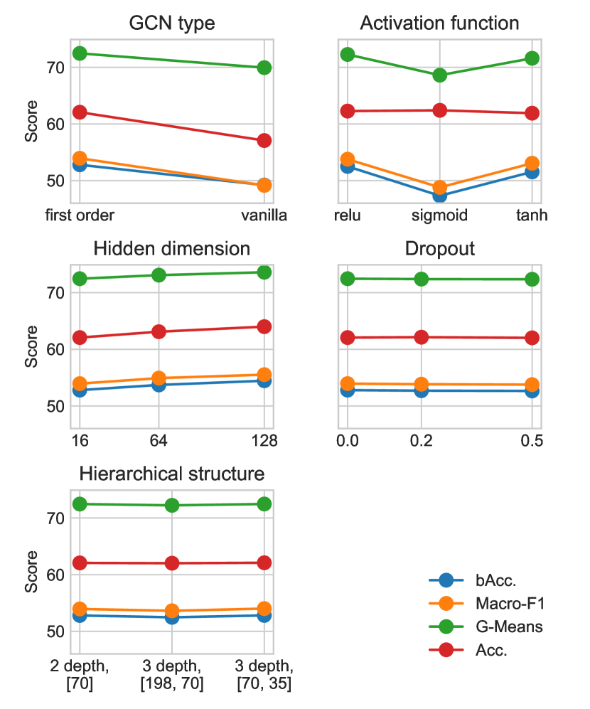
Figure 6. Hyperparameter analysis on Cora-Full.

Hyperparameter Analysis. We study seven hyperparameters of Tail2Learn: (1) the weight $\gamma$ to balance the contribution of three losses; (2) the temperature $\tau$ of balanced contrastive loss in M1; (3) use first-order GCN or vanilla GCN; (4) the activation function in GCN; (5) the number of hidden dimensions; (6) the dropout rate; and (7) the structure of hierarchical graph neural network including the depth and the number $k$ of tasks. The sensitivity analysis on the first two important hyperparameters is given in Figure 5 in Appendix G. It shows the fluctuation of the bAcc (z-axis) is less than 5%. The bAcc is slightly lower when both weight $\gamma$ and temperature $\tau$ become larger. The analysis results for the remaining five hyperparameters are presented in Figure 6. Overall, we find Tail2Learn is reliable and not sensitive to the hyperparameters under a wide range.

Complexity Analysis. We report the running time of Tail2Learn and GCN. To better visualize the performance, we run the experiment on an increasing graph size, i.e., from 1,000 to 30,000 nodes. From Figure 7 in Appendix G, we can see the running time of our model is similarly linear.

5. related work

Long-tail problems. The long-tail distribution of datasets is common in real-world applications, where a small number of classes (i.e., head classes) have majority sample points while the other classes (i.e., tail classes) are only relevant to a small number of samples (Zhang et al., 2021a). Plenty of tasks in diverse research areas suffer from this issue, such as medical image diagnosis (Ju et al., 2021), classification in computer vision (Kang et al., 2020; Tang et al., 2020), and recommendation (Yin et al., 2020; Chen et al., 2020), and there are several efforts focus on solving the long-tail problem (Chawla, 2003; Liu et al., 2008; Chawla et al., 2002; Elkan, 2001; Zhou and Liu, 2005; Yuan and Ma, 2012). In the data-level methods, the vanilla oversampling method (Chawla, 2003; Liu et al., 2008) addresses this problem by replicating existing minority samples. However, it may lead to overfitting because no additional information is introduced. In 2002, Chawla et al. (Chawla et al., 2002) proposed SMOTE to generate new samples by feature interpolation samples of tail classes with their nearest neighbors. In the algorithm-level methods, cost-sensitive methods (Elkan, 2001; Zhou and Liu, 2005; Yuan and Ma, 2012) introduce different cost matrices to assign different misclassification penalties to samples of a specific class. However, the vast majority of previous efforts focus on independent and identically distributed (i.i.d.) data, which cannot be directly applied to graph data.

Recently, several related works for long-tail classification on graphs (Park et al., 2022; Yun et al., 2022; Zhao et al., 2021; Wu et al., 2021a; Shi et al., 2020; Qu et al., 2021; Liu et al., 2021, 2020) have attracted attention. In 2021, Zhao et al. (Zhao et al., 2021) propose the first work named GraphSMOTE considering node class imbalance on graphs. It extends SMOTE to graph-structure data by interpolating tail node embeddings and generating edges utilizing an edge generator pre-trained on the original graph. GraphMixup (Wu et al., 2021a) is a mixup-based framework that implements three-level mixups (feature, edge, and label) concurrently in an end-to-end manner. ImGAGN (Qu et al., 2021) is an adversarial learning-based approach. It uses a generator to simulate minority nodes and topological structure, then uses a discriminator to discriminate between real and fake nodes, and between minority and majority nodes. However, the long-tail class-membership approaches on graphs often lack a theoretical basis. And They are experimented under class imbalance settings: for class imbalance learning, the number of classes can be small, and the number of minority nodes may not be small; but for long-tail learning, the number of classes is large, and the tail nodes are scarce. Here we consider a measure of the long-tail distribution of node classes and conduct experiments on the long-tail datasets.

Graph Neural Networks. Graph neural networks emerge as state-of-the-art methods for graph representation learning, which capture the structure of graphs via the key operation of message passing between nodes. Many significant efforts such as GCN (Kipf and Welling, 2017), GraphSAGE (Hamilton et al., 2017), GIN (Xu et al., 2019), and GAT (Veličković et al., 2018) arose and have become indispensable baselines in a wide range of downstream tasks. For a more elaborate discussion on the wide range of GNNs, we refer readers to excellent recent surveys (Wu et al., 2020; Zhou et al., 2020). Recently, several attempts have been focused on extending pooling operations to graphs. In order to achieve an overview of the graph structure, hierarchical pooling (Ma et al., 2019; Ranjan et al., 2020; Lee et al., 2019; Ying et al., 2018; Gao and Ji, 2019) techniques attempt to gradually group nodes into clusters and coarsen the graph recursively. DiffPool (Ying et al., 2018) utilizes a dense assignment matrix to softly assign nodes to a set of clusters in the following layer. SAGPool (Lee et al., 2019) developes a top-K node selection method to generate an induced subgraph for the following input layer. Graph U-Nets (Gao and Ji, 2019) proposes a similar encoder-decoder architecture based on gPool and gUnpool layers. However, these approaches are generally designed to enhance the representation of the whole graph. In this paper, we aim to explore node classification with the long-tail class-membership distribution via hierarchical pooling methods.

6. conclusion

In this paper, we investigate long-tail classification on graphs, which intends to improve the performance on both head and tail classes. By formulating this problem in the fashion of multi-task learning, we propose the first generalization bound dominated by the range of losses across all tasks and the total number of tasks. Building upon the theoretical findings, we also present Tail2Learn. It is an generic framework with two major modules: M1. Hierarchical task grouping to address C2 (Label scarcity) and C3 (Task complexity); and M2. Long-tail balanced contrastive learning to solve C1 (High-skewed data distribution). Extensive experiments on six real-world datasets, where Tail2Learn consistently outperforms state-of-art baselines, demonstrate the efficacy of our model for capturing long-tail categories on graphs.

Reproducibility: We have released our code and data at https://anonymous.4open.science/r/Tail2Learn-CE08/.

Appendix A Symbols and notations

Here we give the main symbols and notations in this paper.

Table 4. Symbols and notations.

Symbol	Description
$\mathcal{G}$	input graph.
$\mathcal{V}$	the set of nodes in $\mathcal{G}$.
$\mathcal{E}$	the set of edges in $\mathcal{G}$.
$\mathbf{X}$	the node feature matrix of $\mathcal{G}$.
$\mathbf{Z}$	the node embeddings in $\mathcal{G}$.
$\mathbf{A}$	the adjacency matrix in $\mathcal{G}$.
$\mathcal{Y}$	the set of labels in $\mathcal{G}$.
$n$	the number of nodes $|\mathcal{V}|$.
$T$	the number of categories of nodes $\mathcal{V}$.
$\texttt{Ratio}_{LT}$	the long-tailedness ratio.

Appendix B Proofs of the Theorems

See 2

Proof.

First, we consider a special case, let $T=1$, we have $\mathbb{E}_{\mathbf{X}\sim\mu_{t}}[f_{t}(\mathbf{X})]-\sum_{i}\frac{1}{n_{t}}f_{t}(\mathbf{x}^{t}_{i})\leq\frac{\sqrt{2\pi}G(\mathcal{Y})}{n_{t}}+\sqrt{\frac{9\ln(2/\delta)}{2n_{t}}}$ following (Maurer et al., 2016). Next, we generalize it and perform the summation operation with respect to $t$. Then we complete the proof. ∎

See 3

See 4

Proof.

Let

(15) $$R(\mathcal{F})=\sup_{\mathbf{y},\mathbf{y}^{\prime}\in\mathcal{Y},\mathbf{y}\neq\mathbf{y}^{\prime}}\mathbb{E}\sup_{f\in\mathcal{F}}\frac{\left\langle\gamma,l\left(f(\mathbf{y})-f(\mathbf{y}^{\prime})\right)\right\rangle}{\left\|\mathbf{y}-\mathbf{y}^{\prime}\right\|}.$$

where $\gamma$ is a vector of independent standard normal variables. Then following the definition of Rademacher complexity and the chain rule given in (Maurer et al., 2016), we have

(16) $$G(\mathcal{F}(\mathcal{Y}))\leq c_{1}L(\mathcal{F})G(\mathcal{Y})+c_{2}D(\mathcal{Y})R(\mathcal{F})+G\left(\mathcal{F}\left(y_{0}\right)\right)$$

where $c_{1}$ and $c_{2}$ are constants. Furthermore,

(17) $$\sup_{\mathbf{y},\mathbf{y}^{\prime}\in\mathcal{Y},\mathbf{y}\neq\mathbf{y}^{\prime}}\mathbb{E}\sup_{f\in\mathcal{F}}\frac{\left\langle\gamma,l\left(f(\mathbf{y})-f(\mathbf{y}^{\prime})\right)\right\rangle}{\left\|\mathbf{y}-\mathbf{y}^{\prime}\right\|}$$

$$\leq \sup_{\mathbf{y},\mathbf{y}^{\prime}\in\mathcal{Y},\mathbf{y}\neq\mathbf{y}^{\prime}}\mathbb{E}\left[\sup_{f\in\mathcal{F}}\left\langle\gamma,l\left(f(\mathbf{y})-y)\right)\right\rangle-\sup_{f\in\mathcal{F}}\left\langle\gamma,l\left(f(\mathbf{y}^{\prime})-y^{\prime})\right)\right\rangle\right]$$

$$\leq \sup_{\mathbf{y},\mathbf{y}^{\prime}\in\mathcal{Y},\mathbf{y}\neq\mathbf{y}^{\prime}}\left[\frac{1}{n}\sum l(f(h(\mathbf{X})),\mathbf{y})-\frac{1}{n}\sum l(f(h(\mathbf{X}^{\prime})),\mathbf{y}^{\prime})\right]$$

$$\leq \max_{t}\frac{1}{n_{t}}\sum_{i=1}^{n_{t}}l(f_{t}(h(\mathbf{x}^{t}_{i})),y^{t}_{i})-\min_{t}\frac{1}{n_{t}}\sum_{i=1}^{n_{t}}l(f_{t}(h(\mathbf{x}^{t}_{i})),y^{t}_{i})$$

Then we complete the proof. ∎

See 5

Proof.

By lemma 2, we have that

(18) $$\mathcal{E}-\hat{\mathcal{E}}\leq\sum_{t}\left(\frac{\sqrt{2\pi}G(S)}{n_{t}}+\sqrt{\frac{9\ln(2/\delta)}{2n_{t}}}\right)$$

where $S=\left\{\left(l(f_{t}(h(X^{t}_{i})),Y^{t}_{i})\right):f_{t}\in\mathcal{F}\right.and\left.h\in\mathcal{H}\right\}\subseteq\mathbb{R}^{n}$. By the Lipschitz property of the loss function $l(\cdot,\cdot)$ and the contraction lemma 3, we have $G(S)\leq G\left(S^{\prime}\right)$, where $S^{\prime}=\left\{\left(f_{t}(h(X^{t}_{i}))\right):f_{t}\in\mathcal{F}\right.\\ and\left.h\in\mathcal{H}\right\}\subseteq\mathbb{R}^{n}$. Then

(19) $$\mathcal{E}-\hat{\mathcal{E}}\leq\sum_{t}\left(\frac{\sqrt{2\pi}G(S^{\prime})}{n_{t}}+\sqrt{\frac{9\ln(2/\delta)}{2n_{t}}}\right).$$

Recall that $\mathcal{H}(\mathbf{X})\subseteq\mathbb{R}^{Kn}$ is defined by

(20) $$\mathcal{H}(\mathbf{X})=\left\{\left(h_{k}(X^{t}_{i})\right):h\in\mathcal{H}\right\},$$

and define a class of functions $\mathcal{F}^{\prime}:\mathbb{R}^{Kn}\rightarrow\mathbb{R}^{n}$ by

(21) $$\mathcal{F}^{\prime}=\left\{y\in\mathbb{R}^{Kn}\mapsto\left(f_{t}(y^{t}_{i})\right):f_{1},\ldots,f_{T}\in\mathcal{F}\right\}.$$

We have $S^{\prime}=\mathcal{F}^{\prime}(\mathcal{H}(\mathbf{X}))$. By Lemma 4 for universal constants $c_{1}^{\prime}$ and $c_{2}^{\prime}$

(22) $$G\left(S^{\prime}\right) \leq c_{1}^{\prime}L\left(\mathcal{F}^{\prime}\right)G(\mathcal{H}(\mathbf{X}))+c_{2}^{\prime}D(\mathcal{H}(\mathbf{X}))\texttt{Range}(f_{1}^{\prime},\ldots,f_{T}^{\prime})$$

$$+\min_{y\in Y}G(\mathcal{F}(y)).$$

We now bound the individual terms on the right-hand side above. Let $y,y^{\prime}\in\mathbb{R}^{Kn}$, where $y=\{y^{t}_{i}\}$ with $y^{t}_{i}\in\mathbb{R}^{K}$ and $y^{\prime}=\{y_{i}^{t\prime}\}$ with $y_{i}^{t\prime}\in\mathbb{R}^{K}$. Then for $f_{1},\ldots,f_{T}\in\mathcal{F}$

(23) $$\left\|f(y)-f(y^{\prime})\right\|^{2} =\sum\left(f_{t}(y^{t}_{i})-f_{t}(y_{i}^{t\prime})\right)^{2}$$

$$\leq L^{2}\sum\left\|y^{t}_{i}-y_{i}^{t\prime}\right\|^{2}=L^{2}\left\|y-y^{\prime}\right\|^{2}$$

so that $L(\mathcal{F}^{\prime})\leq L$. Next, we take $y_{0}=0$ and the last term in (22) vanishes because we have $f(0)=0$ for all $f\in\mathcal{F}$. Substitution in (22) and using $G(S)\leq G(S^{\prime})$, we have

(24) $$G(S)\leq c_{1}^{\prime}LG(\mathcal{H}(\mathbf{X}))+c_{2}^{\prime}\sqrt{T}D(\mathcal{H}(\mathbf{X}))\texttt{Range}(f_{1},\ldots,f_{T}).$$

Finally, we bound $D(\mathcal{H}(\mathbf{X}))\leq 2\sup_{h}\|h(\mathbf{X})\|$ and substitution in (18), the proof is completed. ∎

See 6

Proof.

Since we have $\texttt{Range}(\mathcal{F}^{(l+1)})<\texttt{Range}(\mathcal{F}^{(l)})$, to compare the two upper bounds, we only need to compare the relationship between $\sum_{t}\frac{1}{n_{t}^{(l+1)}}$ and $\sum_{t}\frac{1}{n_{t}^{(l)}}$. Consider a special case where we group the tasks $1,\cdots,t$ to the same hypertask in the $l^{\text{th}}$ layer. Then we have $t$ tasks in layer $(l)$ and the number of nodes belonging to task $t$ is $n_{t}$; one task in layer $(l+1)$ and the number of nodes contained in this task is $n_{1}+n_{2}+\cdots+n_{t}$. According to the relationship between the reconciled mean and the arithmetic mean, we have

(25) $$\frac{1}{n_{1}+n_{2}+\cdots+n_{t}}\leq \frac{t^{2}}{n_{1}+n_{2}+\cdots+n_{t}}$$

$$\leq \frac{1}{n_{1}}+\frac{1}{n_{2}}+\cdots+\frac{1}{n_{t}}.$$

Without loss of generality, we have $\sum_{t}\frac{1}{n_{t}^{(l+1)}}\leq\sum_{t}\frac{1}{n_{t}^{(l)}}$, the proof is completed. ∎

Appendix C Pseudo-Code

In this section, we provide the pseudo-code of Tail2Learn.

Algorithm 1 The Tail2Learn Learning Framework.

0:    an input graph $\mathcal{G}=(\mathcal{V},\mathcal{E},\mathbf{X})$ with small node class long-tail ratio $\texttt{Ratio}_{LT}(\alpha)$ and few-shot annotated data $\mathcal{Y}$.

0:    Accurate predictions $\hat{\mathcal{Y}}$ of unlabeled nodes in the graph $\mathcal{G}$

1:   Initialize GCNs for graph embedding layer, task grouping layers, and unpooling layers; the MLP for the node classification task in $\mathcal{G}$.

2:  while not converge do

3:      Compute node representations in a low-dimensional space of $\mathcal{G}$ via GCN for graph embedding layer.

4:     for layer $l\in\{1,\ldots,L\}$ do

5:         Generate a down-sampling new graph (Eq. (8)) and compute node representations for the new graph by $l^{\text{th}}$ task grouping layer.

6:     end for

7:     for layer $l\in\{1,\ldots,L\}$ do

8:         Restore the original graph resolutions (Eq. (9)) and compute node representations for the origin graph by $l^{\text{th}}$ unpooling layer.

9:     end for

10:      Perform skip-connections between the task grouping and unpooling layers, and calculate final node embeddings by feature addition. Employ an MLP layer for final predictions.

11:      Calculate node classification loss $\mathcal{L}_{NC}$ (Eq. (13)) with node embeddings obtained in Step 3, calculate balanced contrastive loss $\mathcal{L}_{BCL}$ (Eq. (10)) with node embeddings obtained in Step 5, and calculate supervised contrastive loss $\mathcal{L}_{SCL}$ (Eq. (11)) with node embeddings obtained in Step 10. Update the hidden parameters of GCNs and MLP by minimizing the loss function in Eq. (14).

12:  end while

13:   return predicted labels $\hat{\mathcal{Y}}$ for unlabeled nodes in the graph $\mathcal{G}$.

Appendix D Details of Datasets

We give further details and descriptions on the six datasets to supplement Sec. 4.1. (1) Cora-Full is a citation network dataset. Each node represents a paper with a sparse bag-of-words vector as the node attribute. The edge represents the citation relationships between two corresponding papers, and the node category represents the research topic. (2) BlogCatalog is a social network dataset with each node representing a blogger and each edge representing the friendship between bloggers. The node attributes are generated from Deepwalk following (Perozzi et al., 2014). (3) Email is a network constructed from email exchanges in a research institution, where each node represents a member, and each edge represents the email communication between institution members. (4) Wiki is a network dataset of Wikipedia pages, with each node representing a page and each edge denoting the hyperlink between pages. (5) Amazon-Clothing is a product network which contains products in ”Clothing, Shoes and Jewelry” on Amazon, where each node represents a product, and is labeled with low-level product categories for classification. The node attributes are constructed based on the product’s description, and the edges are established based on their substitutable relationship (”also viewed”). (6) Amazon-Electronics is another product network constructed from products in ”Electronics” with nodes, attributes, and labels constructed in the same way. Differently, the edges are created with the complementary relationship (”bought together”) between products.

For additional processing, the first four datasets are randomly sampled according to train/valid/test ratios = 1:1:8 for each category. For the last two datasets, nodes are removed until the category distribution follows a long-tail distribution (here we make the head 20% categories containing 80% of the total nodes) with keeping the connections between the remaining nodes. We sort the categories by the number of nodes they contain and then downsample the tail 80% categories equally. When eliminating nodes, we remove nodes with low degrees and their corresponding edges. After semi-synthetic processing, the long-tailedness ratio of order 0.8 ($\texttt{Ratio}_{LT}(0.8)$) of train set is approximately equal to 0.25. For valid/test sets, we sample 25/55 nodes from each category. To sum up, Tail2Learn is evaluated based on four natural datasets, and two additional datasets with semi-synthetic long-tail settings.

The statistics, the original class-imbalance ratio, and original long-tailedness ratio ($\texttt{Ratio}_{LT}(0.8)$ as defined in Definition 1) of each dataset are summarized in Table 5.

Table 5. Dataset statistics.

Dataset	#Nodes	#Edges	#Attributes	#Classes	Imb.	$\texttt{Ratio}_{LT}$
Cora-Full	19,793	146,635	8,710	70	0.016	1.09
BlogCatalog	10,312	333,983	64	38	0.002	0.77
Email	1,005	25,571	128	42	0.009	0.79
Wiki	2,405	25,597	4,973	17	0.022	1.00
Amazon-Clothing	24,919	91,680	9,034	77	0.097	1.23
Amazon-Electronics	42,318	43,556	8,669	167	0.107	1.67

Appendix E Details of Baselines

In this section, we describe each baseline in more details to supplement Sec. 4.1.

Classical long-tail learning methods: Origin utilizes a GCN (Kipf and Welling, 2017) as the encoder and an MLP as the classifier. Over-sampling (Chawla, 2003) duplicates the nodes of tail classes and creates a new adjacency matrix with the connectivity of the oversampled nodes. Re-weighting (Yuan and Ma, 2012) penalizes the tail nodes to compensate for the dominance of the head nodes. SMOTE (Chawla et al., 2002) generates synthetic nodes by feature interpolation tail nodes with their nearest and assigns the edges according to their neighbors’ edges. Embed-SMOTE (Ando and Huang, 2017) performs SMOTE in the embedding space instead of the feature space.

GNN-based long-tail learning methods: GraphSMOTE (Zhao et al., 2021) extends classical SMOTE to graph data by interpolating node embeddings and connecting the generated nodes via a pre-trained edge generator. It has two variants: $\text{GraphSMOTE}_{T}$ and $\text{GraphSMOTE}_{O}$, depending on whether the predicted edges are discrete or continuous. GraphMixup (Wu et al., 2021a) performs semantic feature mixup and contextual edge mixup to capture graph feature and structure and then develops a reinforcement mixup to determine the oversampling ratio for tail classes. ImGAGN (Qu et al., 2021) is an adversarial-based method that uses a generator to simulate minority nodes and a discriminator to discriminate between real and fake nodes. LTE4G (Yun et al., 2022) splits the nodes into four balanced subsets considering class and degree long-tail distributions. Then, it trains an expert for each balanced subset and employs knowledge distillation to obtain the head student and tail student for further classification.

Appendix F Details of Parameter Settings

Here we provide the details of parameter settings. For a fair comparison, we use vanilla GCN as backbone and set the hidden layer dimensions of all GCNs in baselines and Tail2Learn to 128 for Cora-Full, Amazon-Clothing, Amazon-Electronics and 64 for BlogCatalog, Email, Wiki. We use Adam optimizer with learning rate 0.01 and weight deacy $5e-4$ for all models. For the oversampling-based baselines, the number of imbalanced classes is set to be the same as in (Yun et al., 2022). And the scale of upsampling is set to 1.0 as in (Yun et al., 2022), that is, the same number of nodes are oversampled for each tail category. For GraphSMOTE, we set the weight of edge reconstruction loss to $1e-6$ as in the original paper (Zhao et al., 2021). For GraphMixup, we use the same default hyperparameter values as in the original paper (Wu et al., 2021a) except settings of maximum epoch and Adam. For LTE4G, we adopt the best hyperparameter settings reported in the paper (Yun et al., 2022). For our model, the weight $\gamma$ of contrastive loss is selected in $\{0.01,0.1\}$, the temperature $\tau$ of contrastive learning is selected in $\{0.01,0.1,1.0\}$. We set the depth of the hierarchical graph neural network to 3; node embeddings are calculated for the first layer, the number of tasks is set to the number of categories for the second layer, and the number of tasks is half the number of categories for the third layer. In addition, the maximum training epoch for all the models is set to 10000. If there is no additional setting in the original papers, we set the early stop epoch to 1000, i.e., the training stops early if the model performance does not improve in 1000 epochs. All the experiments are conducted on an A100 SXM4 80GB GPU.

Appendix G Details of Parameter and Complexity Analysis

Hyperparameter Analysis: First we show the sensitivity analysis with respect to weight $\gamma$ and temperature $\tau$, and the results are shown in Figure 5. The fluctuation of the bAcc (z-axis) is less than 5%. The bAcc is slightly lower when both weight $\gamma$ and temperature $\tau$ become larger. The detailed analysis results for the remaining four hyperparameters are presented in Appendix G. For analyzing these hyperparameters, all the experiments are conducted with weight $\gamma=0.01$ and temperature $\tau=0.01$. The dimension of hidden layers is set to 16 except for the experiment investigating the hidden layer dimension. For hierarchical structure, we investigated different hierarchical depths and task sizes: (1) using node embeddings and prototype embeddings for 70 (# of classes) tasks; (2) using node embeddings, prototype embeddings for 198 tasks, and prototype embeddings for 70 hypertasks; (3) using node embeddings, prototype embeddings for 70 tasks, and prototype embeddings for 35 hypertasks. From the experimental results, we can see that our model is insensitive to hyperparameters.

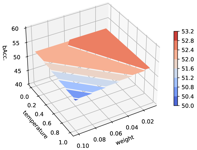
Figure 5. Hyperparameter analysis on Cora-Full with respect to weight $\gamma$ and temperature $\tau$.

hyperparameter

appendix hyperparameter

Complexity analysis: For each certain size, we run 10 times using the synthetic dataset. Each point in Figure 7 is computed based on the average value of the 10 runs. We can see the running time of our model is similarly linear.

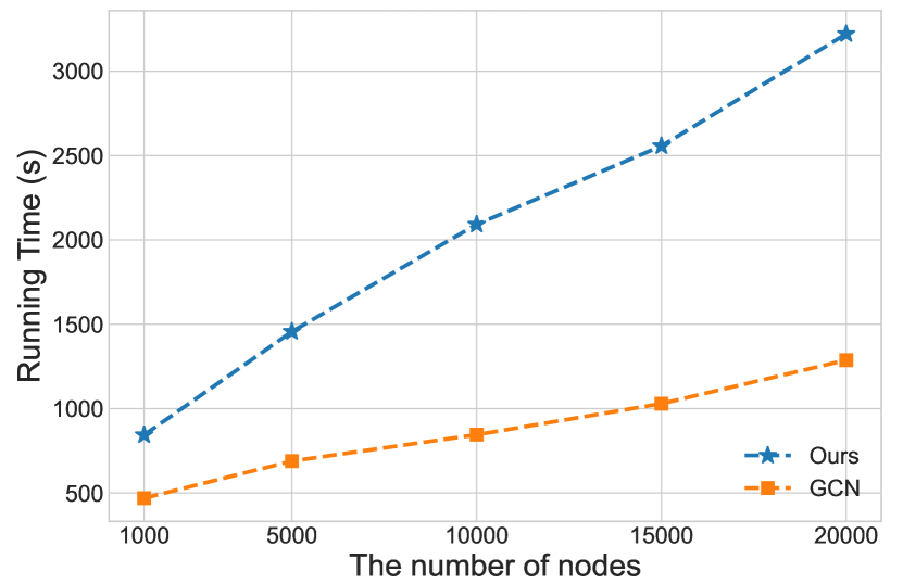
Figure 7. Complexity analysis w.r.t. the number of nodes.

complexity

References

- (1)
- Abu-El-Haija et al. (2020) Sami Abu-El-Haija, Amol Kapoor, Bryan Perozzi, and Joonseok Lee. 2020. N-GCN: Multi-scale Graph Convolution for Semi-supervised Node Classification. In Proceedings of The 35th Uncertainty in Artificial Intelligence Conference (Proceedings of Machine Learning Research, Vol. 115). PMLR, 841–851.
- Akoglu et al. (2015) Leman Akoglu, Hanghang Tong, and Danai Koutra. 2015. Graph based anomaly detection and description: a survey. Data mining and knowledge discovery 29, 3 (2015), 626–688.
- Ando and Huang (2017) Shin Ando and Chun Yuan Huang. 2017. Deep over-sampling framework for classifying imbalanced data. In Joint European Conference on Machine Learning and Knowledge Discovery in Databases. Springer, 770–785.
- Bessadok et al. (2022) Alaa Bessadok, Mohamed Ali Mahjoub, and Islem Rekik. 2022. Graph neural networks in network neuroscience. IEEE Transactions on Pattern Analysis and Machine Intelligence (2022).
- Bojchevski and Günnemann (2018) Aleksandar Bojchevski and Stephan Günnemann. 2018. Deep Gaussian Embedding of Graphs: Unsupervised Inductive Learning via Ranking. In International Conference on Learning Representations.
- Chawla (2003) Nitesh V Chawla. 2003. C4. 5 and imbalanced data sets: investigating the effect of sampling method, probabilistic estimate, and decision tree structure. In Proceedings of the ICML, Vol. 3. CIBC Toronto, ON, Canada, 66.
- Chawla et al. (2002) Nitesh V Chawla, Kevin W Bowyer, Lawrence O Hall, and W Philip Kegelmeyer. 2002. SMOTE: synthetic minority over-sampling technique. Journal of artificial intelligence research 16 (2002), 321–357.
- Chen et al. (2020) Zhihong Chen, Rong Xiao, Chenliang Li, Gangfeng Ye, Haochuan Sun, and Hongbo Deng. 2020. Esam: Discriminative domain adaptation with non-displayed items to improve long-tail performance. In Proceedings of the 43rd International ACM SIGIR Conference on Research and Development in Information Retrieval. 579–588.
- Choi et al. (2017) Edward Choi, Mohammad Taha Bahadori, Le Song, Walter F Stewart, and Jimeng Sun. 2017. GRAM: graph-based attention model for healthcare representation learning. In Proceedings of the 23rd ACM SIGKDD international conference on knowledge discovery and data mining. 787–795.
- Dou et al. (2020) Yingtong Dou, Zhiwei Liu, Li Sun, Yutong Deng, Hao Peng, and Philip S. Yu. 2020. Enhancing Graph Neural Network-Based Fraud Detectors against Camouflaged Fraudsters. In Proceedings of the 29th ACM International Conference on Information and Knowledge Management (CIKM ’20). 315–324.
- Elkan (2001) Charles Elkan. 2001. The foundations of cost-sensitive learning. In International joint conference on artificial intelligence, Vol. 17. Lawrence Erlbaum Associates Ltd, 973–978.
- Fan et al. (2019) Wenqi Fan, Yao Ma, Qing Li, Yuan He, Eric Zhao, Jiliang Tang, and Dawei Yin. 2019. Graph Neural Networks for Social Recommendation. In The World Wide Web Conference (WWW ’19). Association for Computing Machinery, 417–426.
- Gao and Ji (2019) Hongyang Gao and Shuiwang Ji. 2019. Graph U-Nets. In International Conference on Machine Learning. 2083–2092.
- Garcia and Bruna (2017) Victor Garcia and Joan Bruna. 2017. Few-shot learning with graph neural networks. arXiv preprint arXiv:1711.04043 (2017).
- Hamilton et al. (2017) Will Hamilton, Zhitao Ying, and Jure Leskovec. 2017. Inductive representation learning on large graphs. Advances in neural information processing systems 30 (2017).
- Hassani and Khasahmadi (2020) Kaveh Hassani and Amir Hosein Khasahmadi. 2020. Contrastive Multi-View Representation Learning on Graphs. In Proceedings of International Conference on Machine Learning. 3451–3461.
- Hearst et al. (1998) Marti A. Hearst, Susan T Dumais, Edgar Osuna, John Platt, and Bernhard Scholkopf. 1998. Support vector machines. IEEE Intelligent Systems and their applications 13, 4 (1998), 18–28.
- Hu et al. (2019) Weihua Hu, Bowen Liu, Joseph Gomes, Marinka Zitnik, Percy Liang, Vijay Pande, and Jure Leskovec. 2019. Strategies for pre-training graph neural networks. arXiv preprint arXiv:1905.12265 (2019).
- Ju et al. (2021) Lie Ju, Xin Wang, Lin Wang, Tongliang Liu, Xin Zhao, Tom Drummond, Dwarikanath Mahapatra, and Zongyuan Ge. 2021. Relational Subsets Knowledge Distillation for Long-Tailed Retinal Diseases Recognition. In International Conference on Medical Image Computing and Computer-Assisted Intervention (Strasbourg, France). Springer-Verlag, Berlin, Heidelberg, 3–12. https://doi.org/10.1007/978-3-030-87237-3_1
- Kang et al. (2020) Bingyi Kang, Saining Xie, Marcus Rohrbach, Zhicheng Yan, Albert Gordo, Jiashi Feng, and Yannis Kalantidis. 2020. Decoupling Representation and Classifier for Long-Tailed Recognition. In International Conference on Learning Representations.
- Kim et al. (2019) Jongmin Kim, Taesup Kim, Sungwoong Kim, and Chang D. Yoo. 2019. Edge-Labeling Graph Neural Network for Few-Shot Learning. In Proceedings of the IEEE/CVF Conference on Computer Vision and Pattern Recognition (CVPR).
- Kingma and Ba (2015) Diederik P. Kingma and Jimmy Ba. 2015. Adam: A Method for Stochastic Optimization. In 3rd International Conference on Learning Representations, ICLR 2015, San Diego, CA, USA, May 7-9, 2015, Conference Track Proceedings.
- Kipf and Welling (2016) Thomas N Kipf and Max Welling. 2016. Semi-supervised classification with graph convolutional networks. arXiv preprint arXiv:1609.02907 (2016).
- Kipf and Welling (2017) Thomas N. Kipf and Max Welling. 2017. Semi-Supervised Classification with Graph Convolutional Networks. In International Conference on Learning Representations.
- Lee et al. (2019) Junhyun Lee, Inyeop Lee, and Jaewoo Kang. 2019. Self-Attention Graph Pooling. In Proceedings of the 36th International Conference on Machine Learning. PMLR, 3734–3743.
- Liu et al. (2008) Xu-Ying Liu, Jianxin Wu, and Zhi-Hua Zhou. 2008. Exploratory undersampling for class-imbalance learning. IEEE Transactions on Systems, Man, and Cybernetics, Part B (Cybernetics) 39, 2 (2008), 539–550.
- Liu et al. (2021) Zemin Liu, Trung-Kien Nguyen, and Yuan Fang. 2021. Tail-GNN: Tail-node graph neural networks. In Proceedings of the 27th ACM SIGKDD Conference on Knowledge Discovery & Data Mining. 1109–1119.
- Liu et al. (2020) Zemin Liu, Wentao Zhang, Yuan Fang, Xinming Zhang, and Steven C.H. Hoi. 2020. Towards Locality-Aware Meta-Learning of Tail Node Embeddings on Networks. In Proceedings of the 29th ACM International Conference on Information and Knowledge Management (Virtual Event, Ireland) (CIKM ’20). Association for Computing Machinery, New York, NY, USA, 975–984. https://doi.org/10.1145/3340531.3411910
- Ma et al. (2019) Yao Ma, Suhang Wang, Charu C. Aggarwal, and Jiliang Tang. 2019. Graph Convolutional Networks with EigenPooling. In Proceedings of the 25th ACM SIGKDD International Conference on Knowledge Discovery & Data Mining (Anchorage, AK, USA) (KDD ’19). ACM, New York, NY, USA, 723–731. https://doi.org/10.1145/3292500.3330982
- Maurer et al. (2016) Andreas Maurer, Massimiliano Pontil, and Bernardino Romera-Paredes. 2016. The Benefit of Multitask Representation Learning. 17, 1 (jan 2016), 2853–2884.
- McAuley et al. (2015) Julian McAuley, Rahul Pandey, and Jure Leskovec. 2015. Inferring networks of substitutable and complementary products. In Proceedings of the 21th ACM SIGKDD international conference on knowledge discovery and data mining. 785–794.
- Mernyei and Cangea (2020) Péter Mernyei and Cătălina Cangea. 2020. Wiki-CS: A Wikipedia-Based Benchmark for Graph Neural Networks. arXiv preprint arXiv:2007.02901 (2020).
- Mittal et al. (2021) Anshul Mittal, Kunal Dahiya, Sheshansh Agrawal, Deepak Saini, Sumeet Agarwal, Purushottam Kar, and Manik Varma. 2021. Decaf: Deep extreme classification with label features. In Proceedings of the 14th ACM International Conference on Web Search and Data Mining. 49–57.
- Oord et al. (2018) Aaron van den Oord, Yazhe Li, and Oriol Vinyals. 2018. Representation learning with contrastive predictive coding. arXiv preprint arXiv:1807.03748 (2018).
- Pareto et al. (1971) Vilfredo Pareto et al. 1971. Manual of political economy. (1971).
- Park et al. (2022) Joonhyung Park, Jaeyun Song, and Eunho Yang. 2022. GraphENS: Neighbor-Aware Ego Network Synthesis for Class-Imbalanced Node Classification. In International Conference on Learning Representations.
- Pelleg and Moore (2004) Dan Pelleg and Andrew Moore. 2004. Active learning for anomaly and rare-category detection. Advances in neural information processing systems 17 (2004).
- Perozzi et al. (2014) Bryan Perozzi, Rami Al-Rfou, and Steven Skiena. 2014. DeepWalk: Online Learning of Social Representations. In Proceedings of the 20th ACM SIGKDD International Conference on Knowledge Discovery and Data Mining (New York, New York, USA) (KDD ’14). Association for Computing Machinery, New York, NY, USA, 701–710. https://doi.org/10.1145/2623330.2623732
- Qiu et al. (2020) Jiezhong Qiu, Qibin Chen, Yuxiao Dong, Jing Zhang, Hongxia Yang, Ming Ding, Kuansan Wang, and Jie Tang. 2020. Gcc: Graph contrastive coding for graph neural network pre-training. In Proceedings of the 26th ACM SIGKDD International Conference on Knowledge Discovery & Data Mining. 1150–1160.
- Qu et al. (2021) Liang Qu, Huaisheng Zhu, Ruiqi Zheng, Yuhui Shi, and Hongzhi Yin. 2021. ImGAGN: Imbalanced network embedding via generative adversarial graph networks. In Proceedings of the 27th ACM SIGKDD Conference on Knowledge Discovery & Data Mining. 1390–1398.
- Ranjan et al. (2020) Ekagra Ranjan, Soumya Sanyal, and Partha Talukdar. 2020. Asap: Adaptive structure aware pooling for learning hierarchical graph representations. In Proceedings of the AAAI Conference on Artificial Intelligence, Vol. 34. 5470–5477.
- Shi et al. (2020) Min Shi, Yufei Tang, Xingquan Zhu, David Wilson, and Jianxun Liu. 2020. Multi-Class Imbalanced Graph Convolutional Network Learning. In Proceedings of the Twenty-Ninth International Joint Conference on Artificial Intelligence, IJCAI-20, Christian Bessiere (Ed.). International Joint Conferences on Artificial Intelligence Organization, 2879–2885. https://doi.org/10.24963/ijcai.2020/398 Main track.
- Singleton and Singleton (2010) Tommie W Singleton and Aaron J Singleton. 2010. Fraud auditing and forensic accounting. Vol. 11. John Wiley & Sons.
- Song et al. (2022) Xiaozhuang Song, Shun Zheng, Wei Cao, James Yu, and Jiang Bian. 2022. Efficient and effective multi-task grouping via meta learning on task combinations. In Advances in Neural Information Processing Systems.
- Tang et al. (2020) Kaihua Tang, Jianqiang Huang, and Hanwang Zhang. 2020. Long-Tailed Classification by Keeping the Good and Removing the Bad Momentum Causal Effect. In Advances in Neural Information Processing Systems, H. Larochelle, M. Ranzato, R. Hadsell, M.F. Balcan, and H. Lin (Eds.), Vol. 33. Curran Associates, Inc., 1513–1524.
- Tang and Liu (2009) Lei Tang and Huan Liu. 2009. Relational Learning via Latent Social Dimensions. In Proceedings of the 15th ACM SIGKDD International Conference on Knowledge Discovery and Data Mining (Paris, France) (KDD ’09). Association for Computing Machinery, New York, NY, USA, 817–826. https://doi.org/10.1145/1557019.1557109
- Veličković et al. (2018) Petar Veličković, Guillem Cucurull, Arantxa Casanova, Adriana Romero, Pietro Liò, and Yoshua Bengio. 2018. Graph Attention Networks. In International Conference on Learning Representations.
- Wang et al. (2019b) Daixin Wang, Jianbin Lin, Peng Cui, Quanhui Jia, Zhen Wang, Yanming Fang, Quan Yu, Jun Zhou, Shuang Yang, and Yuan Qi. 2019b. A semi-supervised graph attentive network for financial fraud detection. In 2019 IEEE International Conference on Data Mining (ICDM). IEEE, 598–607.
- Wang et al. (2019a) Xiang Wang, Xiangnan He, Yixin Cao, Meng Liu, and Tat-Seng Chua. 2019a. KGAT: Knowledge Graph Attention Network for Recommendation. In Proceedings of the 25th ACM SIGKDD International Conference on Knowledge Discovery and Data Mining (KDD ’19). Association for Computing Machinery, New York, NY, USA, 950–958.
- Wang et al. (2021) Yiwei Wang, Wei Wang, Yuxuan Liang, Yujun Cai, and Bryan Hooi. 2021. Mixup for node and graph classification. In Proceedings of the Web Conference 2021. 3663–3674.
- Wu et al. (2021b) Jiancan Wu, Xiang Wang, Fuli Feng, Xiangnan He, Liang Chen, Jianxun Lian, and Xing Xie. 2021b. Self-Supervised Graph Learning for Recommendation. In Proceedings of the 44th International ACM SIGIR Conference on Research and Development in Information Retrieval (SIGIR ’21). Association for Computing Machinery, 726–735.
- Wu et al. (2021a) Lirong Wu, Haitao Lin, Zhangyang Gao, Cheng Tan, Stan Li, et al. 2021a. Graphmixup: Improving class-imbalanced node classification on graphs by self-supervised context prediction. arXiv preprint arXiv:2106.11133 (2021).
- Wu et al. (2020) Zonghan Wu, Shirui Pan, Fengwen Chen, Guodong Long, Chengqi Zhang, and S Yu Philip. 2020. A comprehensive survey on graph neural networks. IEEE transactions on neural networks and learning systems 32, 1 (2020), 4–24.
- Xu et al. (2021) Dongkuan Xu, Wei Cheng, Dongsheng Luo, Haifeng Chen, and Xiang Zhang. 2021. InfoGCL: Information-Aware Graph Contrastive Learning. In Advances in Neural Information Processing Systems, Vol. 34. 30414–30425.
- Xu et al. (2019) Keyulu Xu, Weihua Hu, Jure Leskovec, and Stefanie Jegelka. 2019. How Powerful are Graph Neural Networks?. In International Conference on Learning Representations.
- Yang et al. (2020) Ling Yang, Liangliang Li, Zilun Zhang, Xinyu Zhou, Erjin Zhou, and Yu Liu. 2020. DPGN: Distribution Propagation Graph Network for Few-Shot Learning. In Proceedings of the IEEE/CVF Conference on Computer Vision and Pattern Recognition (CVPR).
- Yin et al. (2017) Hao Yin, Austin R. Benson, Jure Leskovec, and David F. Gleich. 2017. Local Higher-Order Graph Clustering. In Proceedings of the 23rd ACM SIGKDD International Conference on Knowledge Discovery and Data Mining (Halifax, NS, Canada) (KDD ’17). Association for Computing Machinery, New York, NY, USA, 555–564.
- Yin et al. (2020) Jianwen Yin, Chenghao Liu, Weiqing Wang, Jianling Sun, and Steven CH Hoi. 2020. Learning transferrable parameters for long-tailed sequential user behavior modeling. In Proceedings of the 26th ACM SIGKDD International Conference on Knowledge Discovery & Data Mining. 359–367.
- Ying et al. (2018) Rex Ying, Jiaxuan You, Christopher Morris, Xiang Ren, William L. Hamilton, and Jure Leskovec. 2018. Hierarchical Graph Representation Learning with Differentiable Pooling. In Proceedings of the 32nd International Conference on Neural Information Processing Systems (Montréal, Canada) (NIPS’18). Curran Associates Inc., Red Hook, NY, USA, 4805–4815.
- Yuan and Ma (2012) Bo Yuan and Xiaoli Ma. 2012. Sampling+ reweighting: Boosting the performance of AdaBoost on imbalanced datasets. In The 2012 international joint conference on neural networks (IJCNN). IEEE, 1–6.
- Yun et al. (2022) Sukwon Yun, Kibum Kim, Kanghoon Yoon, and Chanyoung Park. 2022. LTE4G: Long-Tail Experts for Graph Neural Networks. In Proceedings of the 31st ACM International Conference on Information & Knowledge Management. 2434–2443.
- Zhang et al. (2021b) Hengrui Zhang, Qitian Wu, Junchi Yan, David Wipf, and Philip S. Yu. 2021b. From Canonical Correlation Analysis to Self-supervised Graph Neural Networks. In Advances in Neural Information Processing Systems, A. Beygelzimer, Y. Dauphin, P. Liang, and J. Wortman Vaughan (Eds.).
- Zhang and Zhou (2013) Min-Ling Zhang and Zhi-Hua Zhou. 2013. A review on multi-label learning algorithms. IEEE transactions on knowledge and data engineering 26, 8 (2013), 1819–1837.
- Zhang and Tong (2016) Si Zhang and Hanghang Tong. 2016. Final: Fast attributed network alignment. In Proceedings of the 22nd ACM SIGKDD international conference on knowledge discovery and data mining. 1345–1354.
- Zhang et al. (2021a) Yifan Zhang, Bingyi Kang, Bryan Hooi, Shuicheng Yan, and Jiashi Feng. 2021a. Deep long-tailed learning: A survey. arXiv preprint arXiv:2110.04596 (2021).
- Zhang et al. (2019) Yingxue Zhang, Soumyasundar Pal, Mark Coates, and Deniz Ustebay. 2019. Bayesian graph convolutional neural networks for semi-supervised classification. In Proceedings of the AAAI conference on artificial intelligence, Vol. 33. 5829–5836.
- Zhao et al. (2021) Tianxiang Zhao, Xiang Zhang, and Suhang Wang. 2021. Graphsmote: Imbalanced node classification on graphs with graph neural networks. In Proceedings of the 14th ACM international conference on web search and data mining. 833–841.
- Zhou et al. (2019) Fan Zhou, Chengtai Cao, Kunpeng Zhang, Goce Trajcevski, Ting Zhong, and Ji Geng. 2019. Meta-gnn: On few-shot node classification in graph meta-learning. In Proceedings of the 28th ACM International Conference on Information and Knowledge Management. 2357–2360.
- Zhou et al. (2020) Jie Zhou, Ganqu Cui, Shengding Hu, Zhengyan Zhang, Cheng Yang, Zhiyuan Liu, Lifeng Wang, Changcheng Li, and Maosong Sun. 2020. Graph neural networks: A review of methods and applications. AI Open 1 (2020), 57–81.
- Zhou and Liu (2005) Zhi-Hua Zhou and Xu-Ying Liu. 2005. Training cost-sensitive neural networks with methods addressing the class imbalance problem. IEEE Transactions on knowledge and data engineering 18, 1 (2005), 63–77.
- Zhu et al. (2022) Jianggang Zhu, Zheng Wang, Jingjing Chen, Yi-Ping Phoebe Chen, and Yu-Gang Jiang. 2022. Balanced Contrastive Learning for Long-Tailed Visual Recognition. In Proceedings of the IEEE/CVF Conference on Computer Vision and Pattern Recognition. 6908–6917.
- Zhu et al. (2021) Yanqiao Zhu, Yichen Xu, Qiang Liu, and Shu Wu. 2021. An Empirical Study of Graph Contrastive Learning. In Thirty-fifth Conference on Neural Information Processing Systems Datasets and Benchmarks Track (Round 2).