Pausing ultrafast melting by multiple femtosecond-laser pulses
Supplemental Material

I Simulation details

The electronic-temperature dependent DFT code CHIVES uses atom-centered Gaussian basis sets and norm-conserving pseudopotentials [1, 2, 3] to describe the electronic system. The exchange and correlation energy is calculated in the local density approximation [4]. After the excitation the electrons do not lose any thermal energy in our simulation, which can be realized by a connection to an infinite heat bath. Therefore, the proper description is the canonical ensemble, in which the free energy $F$ is a constant. On the other hand, the energy can vary, and so we looked at the total energy $E_{\rm{TOT}}(t)$ of the system for the different excitations discussed here (Fig. S1). For clarification, here, the term total energy describes electronic and ionic energies. $E_{0}=3.958\ \mathrm{Ha/atom}$ of the system at $T_{e}=315$ K and $T_{I}=0$ K is used as a reference point. The absorbed energy by the electronic system in an ideal crystal ($T_{I}=0$ K) at a high electronic temperature $T_{e}=14842$ K (purple) and $T_{e}=17368$ K (red) are shown as a reference.

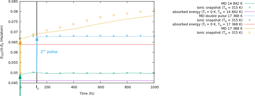
Figure S1: Total energy evolution after the excitation to $T_{e}=14842$ K (green solid line), $T_{e}=17368$ K (gold solid line) by a single pulse and for the double-pulse excitation to $T_{e}=17368$ K (blue solid line). The total energy $E_{0}=3.958\ \mathrm{Ha/atom}$ of the system at $T_{e}=315$ K and $T_{I}=0$ K is used as a reference point. Vertical solid lines represent the absorbed energy in the case of $T_{e}=14842$ K (purple) and $T_{e}=17368$ K (red). The symbols (square and stars) correspond to total energy computations for ionic configuration snapshots of the MD runs, but at an electronic temperature of $T_{e}=315$ K. Therefore, the difference of the total energy between symbols and the corresponding line of the same color is the contribution of the high electronic temperature to the total energy.

The offset of the MD simulation results at $t=0$ fs are due to the initial kinetic energy at $T_{I}=315$ K. By computing the total energy of MD snapshots (positions and velocities) in which the electronic temperature is set to $T_{e}=315$ K (data points at $n\times 100$ fs) we conclude that the time-evolution after the second pulse (blue solid line) can be described very well by the sum of the ionic thermal energy and the absorbed energy (blue stars), just like the case of single-pulse excitation to $T_{e}=14842$ below the melting threshold (green solid line and green stars). This means the system does not extract energy from the heat bath and the electronic-temperature-determined potential energy surface is close to the one at $T_{e}=315$ K. This changes for the single pulse excitation above the nonthermal melting threshold due to fact that the crystal disorders (gold solid line), and the energy rises steadily within the simulation time. In addition, we investigated the potential-energy difference of this laser-induced transition to a metastable phase after the second pulse. To make this comparison, we need two calculations at common $T_{I}$ and $T_{e}$. We use the energies of the ionic snapshots of the system after the second pulse at $1$ ps, with $T_{e}=315$ K and $T_{I}\approx 215$ K (the average, as shown in Fig. 3c), and calculate the total energy difference from a reference system close to the equilibrium structure, which was initialized at $T_{I}=215$ K and $T_{e}=315$ K. The result $\Delta E=0.086\ \mathrm{eV/atom}$ is in the range of energy differences between solid phases in silicon [5].

We use a supercell consisting of $5\times 5\times 5$ conventional unit cells of $8$ atoms each. The unit cell itself has an internal lattice parameter of $5.3987$ Å. Due to the large supercell it is enough to perform simulations in the $\Gamma$-point approximation to obtain convergence. The atomic displacements and velocities are distributed in accordance with a Maxwell distribution at $k_{B}T=1\ \mathrm{mHa},T\approx 315$ K by using true random numbers [6] and the procedure explained in [1]. We generated $N_{run}=10$ molecular-dynamic simulation runs with independent initial ionic conditions. Their trajectories are averaged to obtain the presented quantities, e.g., the mean-square atomic displacement. The time-evolution of the atomic system is modelled by a Velocity-Verlet algorithm using a timestep of $2$ fs, which was already tested in previous studies [1, 7]. For the electronic density of states (EDOS) we used the energy eigenvalues of the system, which were smeared by Gaussians with a FWHM of $0.2$ eV. For all excitations the ionic configuration of the last timestep of our simulation (at $1$ ps) was considered, respectively. For the phonon density of states (PhDOS) we diagonalized the dynamical matrix of the system at $T_{I}=0$ K, no thermal displacements, and high $T_{e}$ for the excited state. For the ground state $T_{e}=315$ K. The phonon eigenvalues are then also smeared by Gaussians with a FWHM of $1$ THz. The eigenvectors $e_{j}$ of the phonons were used to compute particular phonon contributions to the ionic temperature (see main text) or the computation of the effective atomic potential. We found that the difference in the eigenvectors between $T_{e}=14842$ K and $T_{e}=17368$ K is very small and does not lead to different results. Therefore, we show in the main text the results projected onto only the eigenvectors corresponding to $T_{e}=17368$ K.

II Mean-square atomic displacement

As mentioned in the main text, our mechanism is determined by three parameters: the electronic temperature induced by the first pulse, timing $t_{2}$ of the second pulse and its induced electronic temperature above the ultrafast melting threshold. In order to find a parameter set that shows a large effect on the laser-induced disordering, we performed simulations for various sets and computed the mean-square atomic displacement ($msd$) (Fig. S2), which is calculated using the equation

$$msd(t)=\sum_{j}^{N_{run}}\frac{\sum_{i}^{N}\left(\vec{r}^{j}_{i}(t)-\vec{r}_{i}^{0}\right)^{2}}{N}\frac{1}{N_{run}}\;,$$ (1)

where $N_{run}=10$ the number of independent runs, $N=1000$ the number of atoms, $\vec{r}_{i}(t)$ the position vector of atom $i$ at time $t$ and $\vec{r}_{i}^{0}$ the ideal silicon structure at $T=0$ K. Some of the results are shown in Fig. S3. A small and non-changing value of the $msd$ indicates a stopped laser-induced non-thermal, ultrafast melting process. For our parameters presented in the main text, the $msd$ increases after the first pulse but remains constant after the second one. For changes in $t_{2}$ or the induced electronic temperature of the second pulse, we observe that the $msd$ increases significantly after a few hundreds of fs after the double-pulse excitation. The slope at $1$ ps of those additional results implies that our suggested mechanism is not used to the fullest for those other parameters. In such a case the prevention of the laser-induced disordering is achieved for a shorter timescale than by the parameters used in the main text. The $msd$ data shows characteristics similar to the Bragg peak intensities, e.g., the time for the first local maximum of the $msd$ after the first pulse matches the time of the first local minimum of the Bragg peak intensity.

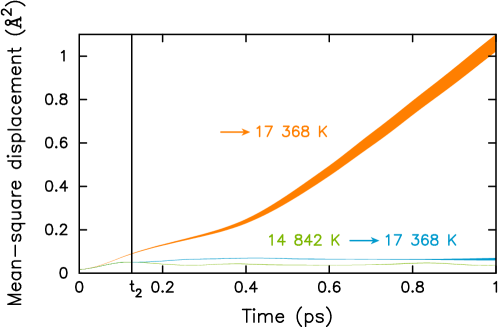
Figure S2: Time-dependence of the mean-square atomic displacement for a single pulse excitation to $T_{e}=14842$ K, our proposed double-pulse excitation to finally $T_{e}=17368$ K, and a single pulse excitation to $T_{e}=17368$ K. The vertical thickness of the lines shows one standard deviation above and below the mean.

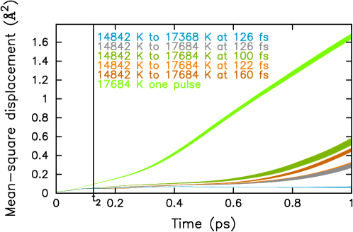
Figure S3: Mean-square displacement data for $t_{2}=100,122,126,160$ fs and $T_{e}=17684$ K. As a reference the ms displacement of $t_{2}=126$ and $T_{e}=17368$ K (light blue) and for the single pulse excitation with $T_{e}=17684$ K is shown (light green).

III Pair-correlation function

In order to obtain specific changes in the crystalline structure after applying our excitation mechanism, we computed the pair-correlation function $g(r)$ directly from the time-dependent atomic positions, by:

$$g(r)=\sum_{i,j}\frac{G(r-r_{ij})}{2\pi r^{2}N}\;.$$ (2)

In this equation, we sum over Gaussians $G$ with a FWHM of 0.1 Å. $r_{ij}$ describes the distance between atom $i$ and $j$. Figure S4 shows $g(r)$ averaged over $10$ independent runs at $t=1$ ps for all induced electronic temperatures studied in this work in comparison to the ground state at $315$ K. The single-pulse excitation below the ultrafast melting threshold ($14842$ K, Fig. S4, top panel, green solid line) causes relatively small changes, mainly in the peak height, but not in the structure of the function. For the single excitation to $17368$ K (Fig. S4, bottom panel, orange solid line) with a single pulse a completely different characteristic is obtained after $1$ ps. The first, main, peak shifted and the structure at longer interatomic distances is completely washed out to an almost constant value around $1$, a clear sign for a crystal symmetry loss. After $1$ ps in the controlled phase, several characteristics are preserved in the presence of extremely hot electrons. In particular, the first peaks remained close to the ground state. Since the first peak corresponds to the nearest neighbor distance, we can conclude that the short-range symmetry is preserved in this case. However, for longer interatomic distances characteristics are slightly washed out, implying the loss of long-range order.

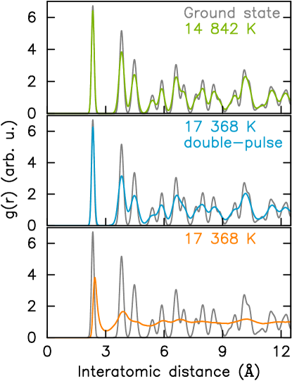
Figure S4: Averaged pair-correlation function $g(r)$ of the ground state initialized with $T=315$ K compared to the system at $t=1$ ps after: (top) a single pulse excitation to $T_{e}=14842$ K, (middle) our proposed double-pulse excitation to a final $T_{e}=17368$ K, and (bottom) a single-pulse excitation to $T_{e}=17368$ K.

IV Additional Bragg Peak intensities

The normalized $(111)$ Bragg peak intensities shown in the main text are computed by

$$I_{hkl}(t)=\frac{1}{N^{2}/2}\left|\sum^{N}_{j=1}e^{-2\pi i\;\left[hx_{j}(t)+kx_{j}(t)+lx_{j}(t)\right]}\right|^{2}\;,$$ (3)

with $(hkl)=(111)$, $N$ the number of silicon atoms in the used supercell, here $1000$, and $x_{j}(t),y_{j}(t),z_{j}(t)$ the time-dependent reduced position of the $j$-th atom. The results shown here are averaged over the trajectories of all ten independent runs. Figs. S5 and S6 present additional results for Bragg intensities other than (111), namely for $(220)$ and $(311)$, respectively. In all of them the effect of preserved crystal symmetry is present.

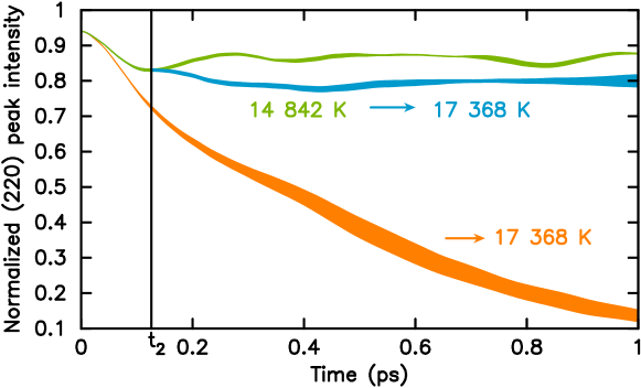
Figure S5: Time-evolution of the (220) Bragg peak intensities for the same laser-induced electronic temperatures as discussed in the main text.

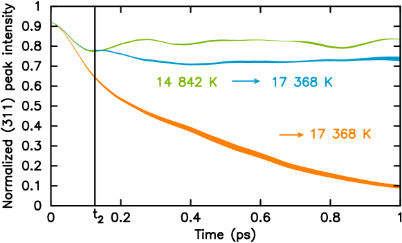
Figure S6: (311) Bragg peak intensity as a function of time after different excitation strengths and mechanisms.

V Structure function

An additional accessible quantity by experiments is the structure function, which we computed in accordance with [7]. We used [8]:

$$I(q,t)=\frac{\sum_{\mathbf{q^{\prime}}}I_{\mathbf{q^{\prime}}}(t)\;G\left(q-q^{\prime}\right)}{\sum_{\mathbf{q^{\prime}}}G\left(q-q^{\prime}\right)}\;,$$ (4)

where $I_{hkl}(t)$ is described by Eq. (3) and $G$ is again a Gaussian with FWHM of $0.2\;\text{\AA}^{-1}$, which we used to smooth the peak intensities. We computed this quantity for each of the individual runs and averaged over $N_{run}$. Fig. S7 shows the results for the controlled phase at $1$ ps after the double pulse excitation and for the ground state. Both data sets are averaged over our ten independent MD-simulation runs. Although plotted with plus-minus the standard deviation, their error is too small to be visible in this figure. In order to make the difference more visible, we additionally plotted the difference of both curves. Whereas all main peaks with corresponding (hkl) decrease in the controlled phase, all intensities between main peaks increase, indicating an increased atomic displacement in the controlled phase than in the ground state.

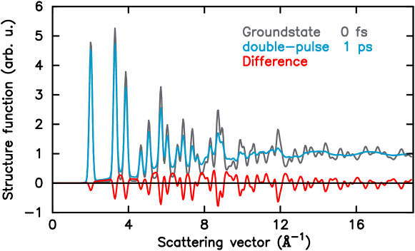
Figure S7: Averaged Structure function as a function of the scattering vector for the ground state (grey solid line) and after $1$ ps in the controlled phase (light blue solid line). For better interpretation, we plotted additionally the difference between both data sets (red solid line).

VI Effective potential-energy surface

In order to get insight into the microscopic mechanisms causing the different outputs described in the main text, we used the ability of the atoms to probe the underlying effective interatomic potential given by DFT. Our MD-simulations provide the time-dependence of the total force $\vec{F}(t)$ and the atomic positions $\vec{r}(t)$. By projecting those quantities on the eigenvector $e_{j}$ of the $j$-th phonon, we obtained for every timestep the force constant $F$ and the displacement $u$ in this particular phonon direction. This data $F(u)$ set is then fitted to a third-order polynomial of the form:

$$F(u)=au^{3}+bu^{2}+cu+d\;,$$ (5)

with real coefficients $a,b,c$ and $d$. We would like to note that for the double-pulse excitation only the time after the second pulse was fitted. The coefficients obtained are summarized in Table S1. For the equilibrium structure at $315$ K a linear fit was sufficient enough to obtain the potential. In this case the atoms do not move far enough to probe any anharmonicities of the potential.

	$a$	$b$	$c$	$d$
	Ha/(bohr)4	Ha/(bohr)3	Ha/(bohr)2	Ha/(bohr)
Equilibrium structure 315 K			$(-5.764\pm 0.006)\times 10^{-3}$	$(-6.7\pm 2.5)\times 10^{-6}$
14842 K	$(6\pm 4)\times 10^{-6}$	$(-6.7\pm 0.4)\times 10^{-6}$	$(-9.55\pm 0.07)\times 10^{-4}$	$(1.1\pm 0.3)\times 10^{-6}$
17368 K (double pulse)	$(4.7\pm 0.5)\times 10^{-6}$	$(-3.3\pm 0.6)\times 10^{-6}$	$(-3.73\pm 0.08)\times 10^{-4}$	$(1.1\pm 0.6)\times 10^{-5}$
17368 K	$(1.6\pm 1.0)\times 10^{-6}$	$(7.4\pm 2.0)\times 10^{-6}$	$(-1.5\pm 0.1)\times 10^{-4}$	$(-1.5\pm 0.9)\times 10^{-5}$

Table S1: Coefficients $a$, $b$, $c$, $d$ of the fitted polynomial of the interatomic forces for the equilibrium structure at $T=315$ K and the three electronic excitations discussed in the main text.

The polynomial fits to the interatomic forces and their error can be seen in Fig. S8.

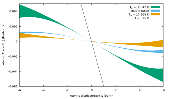
Figure S8: The mean value of the polynomial fit of the interatomic forces for each excitation plus/minus its error by correlated error propagation [9].

The displacement of atoms in the above mentioned phonon direction varies between the runs, because of the different initial conditions. For instance, the direction $+u$ is predominant in one run and $-u$ in another one. As a consequence the effective atomic potential is only probed in this range of $u$, which could lead to different shapes of the fitted force dependencies. Therefore, we plotted the mean value $F(u)$ for every single run in Figs. S9 – S10 (left column) as well as the integrated effective potential energy (right column) for the three excitations described in the main text. With dashed vertical lines we indicate the average atomic displacement range.

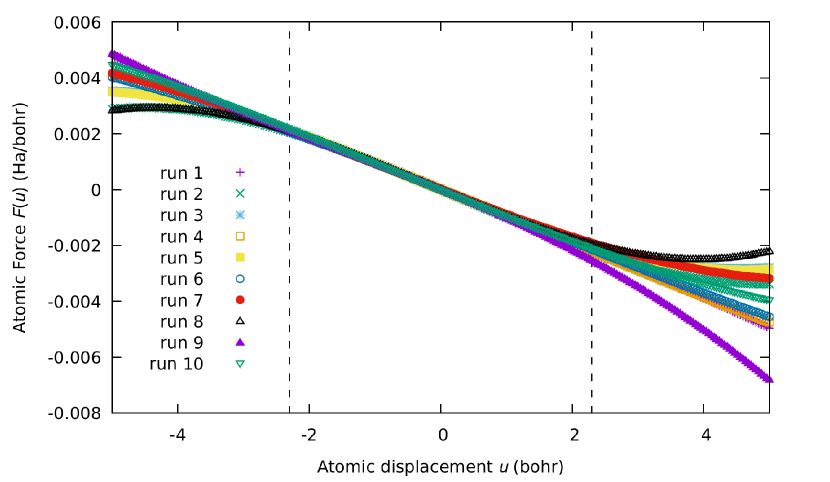
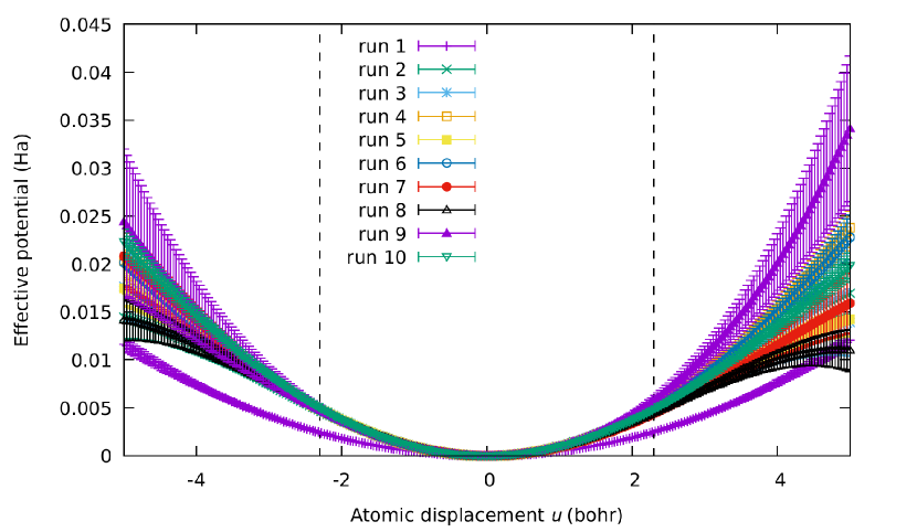
Figure S9: (left) The interatomic fitted forces $F(u)$ for each simulation run (1-10) for $T_{e}=14842$ K. (right) The effective potential energy for the same excitation strength. Vertical dashed lines indicate the average atomic displacement range.

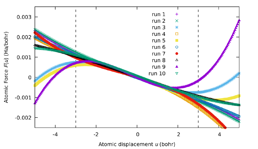
(a)

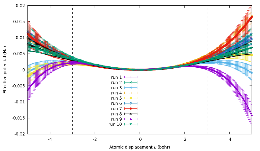
(b)

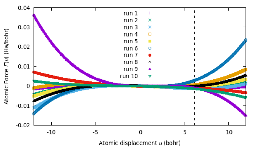
(c)

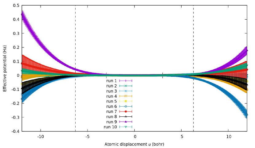
(d)

Figure S10: (a) The interatomic fitted forces $F(u)$ for the double-pulse excitation to $T_{e}=17368$ K for each simulation run (1-10). (b) The effective potential energy for the same excitation strength. (c) $F(u)$ for each simulation run (1-10) for a single-pulse excitation to $T_{e}=17368$ K for a wider atomic displacement range and (d) the corresponding effective potential. Vertical dashed lines indicate the average atomic displacement range.

Two different behaviors can be observed from this data. First, in the vicinity of $u=0$ the characteristics do not vary between the runs; the slope as well as the absolute value of $F$ are the same within each run. This region (ranging from $2$ to $5$ bohr depending on the excitation) seems to be probed by the atoms very accurately. Secondly, for larger $u$, we observe large differences between the fitted forces. This is a direct consequence of the above mentioned fact, that the atoms do not probe the same phase space in each run. In addition, the surrounding configuration is different in each run, which affects the probed effective interatomic force, especially for the laser-induced melting case. Therefore, the value for very large $u$ is not necessarily meaningful for extrapolation. However, the slopes of $F(u)$ observed here verify that after the double-pulse excitation an attractive potential is still present. We note that the linear slope, which corresponds to the harmonic potential, around $u=0$ bohr decreased by $93.6$% compared to the equilibrium structure at $T=315$ K. After the single-pulse excitation to $T_{e}=17368$ K the same slope decreased by $97.4$% and $40.2$% compared to the equilibrium state and the double-pulse excitation, respectively. Therefore, in this case the vicinity of $u=0$ bohr can still be described by an attractive harmonic potential, which is more than a factor of 2 weaker than after the double pulse.

VII Partial ionic temperature

As described in the main text and shown in Fig. 3(a), we decomposed the total ionic temperature using the PhDOS. For completeness we show here the results for a single-pulse excitation to $T_{e}=14842$ K. Here, the different phonon ranges also do not share a common temperature after $1$ ps. However, the difference between the ranges is here only of the order of $30$ to $50$ K.

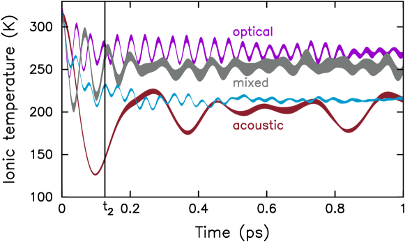
Figure S11: Ionic temperature as a function of time after a laser excitation inducing $T_{e}=14842$ K. It is decomposed in three phonon ranges: acoustic, mixed, optical. As a reference the total ionic temperature for the double pulse excitation is shown (light blue).

References

- Zijlstra et al. [2013] E. S. Zijlstra, A. Kalitsov, T. Zier, and M. E. Garcia, Squeezed thermal phonons precurse nonthermal melting of silicon as a function of fluence, Phys. Rev. X 3, 011005 (2013).
- Zier et al. [2015] T. Zier, E. S. Zijlstra, A. Kalitsov, I. Theodonis, and M. E. Garcia, Signatures of nonthermal melting, Struct. Dyn. 2, 054101 (2015).
- Zier et al. [2016] T. Zier, E. S. Zijlstra, and M. E. Garcia, Quasimomentum-space image for ultrafast melting of silicon, Phys. Rev. Lett. 116, 153901 (2016).
- Perdew and Wang [1992] J. P. Perdew and Y. Wang, Accurate and simple analytic representation of the electron-gas correlation energy, Phys. Rev. B 45, 13244 (1992).
- Malone and Cohen [2012] B. D. Malone and M. L. Cohen, Prediction of a metastable phase of silicon in the Ibam structure, Phys. Rev. B 85, 024116 (2012).
- Haahr [2023] M. Haahr, RANDOM.ORG: true random number service, https://www.random.org (1998–2023).
- Zier et al. [2017] T. Zier, E. S. Zijlstra, S. Krylow, and M. E. Garcia, Simulations of laser-induced dynamics in free-standing thin silicon films, Appl. Phys. A 123, 625 (2017).
- Lin and Zhigilei [2006] Z. Lin and L. V. Zhigilei, Time-resolved diffraction profiles and atomic dynamics in short-pulse laser-induced structural transformations: Molecular dynamics study, Phys. Rev. B 73, 184113 (2006).
- Peralta [2012] M. Peralta, Propagation of Errors: How to Mathematically Predict Measurement Errors (CreateSpace Independent Publishing Platform, 2012).