Degenerate homoclinic bifurcations in complex dimension 2

Abstract.

Unfolding homoclinic tangencies is the main source of bifurcations in 2-dimensional (real or complex) dynamics. When studying this phenomenon, it is common to assume that tangencies are quadratic and unfold with positive speed. Adapting to the complex setting an argument of Takens, we show that any 1-parameter family of 2-dimensional holomorphic diffeomorphisms unfolding an arbitrary non-persistent homoclinic tangency contains such quadratic tangencies. Combining this with recent results of Avila-Lyubich-Zhang and former results in collaboration with Lyubich, this yields the abundance of robust homoclinic tangencies in the bifurcation locus for complex Hénon maps. We also study bifurcations induced by families with persistent tangencies, which provide another approach to the complex Newhouse phenomenon.

1. Introduction

Bifurcation theory is the study of the mechanisms creating instability in smooth dynamics. For surface diffeomorphisms, the most basic such mechanism is the unfolding of a homoclinic tangency, and a long standing conjecture of Palis predicts that homoclinic tangencies are the building block of all bifurcations. Recall that a homoclinic tangency is a tangency between the stable manifold and the unstable manifold of a saddle periodic point. We refer the reader to the classical monograph of Palis and Takens [29] for an introduction to this topic.

When studying the unfolding of a homoclinic tangency, it is common to restrict to a 1-parameter family (or more generally a finite dimensional parameter family) where the unfolding is “as transverse as it can be”, namely that the tangency is quadratic and detaches with positive speed. Without these assumptions, the analysis of the bifurcation becomes much more delicate –the situation is somehow parallel to the difference between the quadratic family and a general multimodal family in one-dimensional dynamics. In the smooth ($C^{k}$) category this restriction is essentially harmless since one can always ensure these properties in a generic family –hence the usual terminology generic homoclinic tangencies. On the other hand, going to the analytic, or even algebraic, category, where the parameter spaces are typically much smaller, the genericity of such tangencies become an interesting problem. In [17], the prevalence of homoclinic tangencies in the space of complex Hénon mappings of a given degree was studied by M. Lyubich and the author, and the Palis conjecture was confirmed under mild dissipativity assumptions. However, the question of the genericity of these tangencies was left open.

In a remarkable, but seemingly not so well-known, paper, Takens [36] proved that in any family of real-analytic surface diffeomorphisms presenting an “inevitable tangency” (that is, in which a tangency must happen for topological reasons), then under a non-degeneracy assumption on the eigenvalues at the saddle point, generic tangencies are dense in the tangency locus. Other relevant references include Robinson [30] and Davis [13], where cascades of sinks are created from tangencies of arbitrary order for real-analytic diffeomorphisms of surfaces (in [30]) and for $C^{\infty}$- diffeomorphisms under a $C^{\infty}$ linearizability condition (in [13]). Many of the techniques developed in these papers take advantage of plane topology and geometry, so non-trivial work needs to be carried out to adapt them to the complex setting. Note that conversely, obtaining degenerate tangencies from non-degenerate ones is also interesting and leads to rich dynamical phenomena (see e.g. [21, 22]).

$\diamond$

The first main result in this paper is a generalization of Takens’ theorem to holomorphic diffeomorphisms.

Theorem A.1.

Let $(f_{\lambda})_{\lambda\in\Lambda}$ be a holomorphic family of holomorphic diffeomorphisms defined in some domain $\Omega\subset{\mathbb{C}^{2}}$, parameterized by a complex manifold $\Lambda$. Assume that in the neighborhood of some $\lambda_{0}\in\Lambda$, $f_{\lambda}$ possesses a saddle fixed point $p_{\lambda}$ with a non persistent homoclinic tangency at ${\lambda_{0}}$. Assume furthermore that there is no persistent relation of the form $u_{\lambda}^{a}s_{\lambda}^{b}=1$, where $s_{\lambda}$ and $u_{\lambda}$ are the respective stable and unstable multipliers of $p_{\lambda}$ and $a$ and $b$ are positive integers.

Then there exists $\lambda_{1}$ arbitrary close to ${\lambda_{0}}$ such that $p_{\lambda_{1}}$ has a quadratic homoclinic tangency, unfolding with positive speed.

Note that the notion of “unfolding with positive speed” really makes sense only if $\Lambda$ is 1-dimensional (see §3 for a thorough discussion). For higher dimensional families, this means that there is a 1-dimensional family though ${\lambda_{0}}$ in which this property holds. Hence the result is strongest when $\Lambda$ is 1-dimensional, and we will prove it in this case. We note that in the quadratic case, the “positive speed” assertion of the theorem was independently established in [3].

To understand the subtlety of this result we have to recall how secondary tangencies are produced from the unfolding of an initial homoclinic tangency. The mechanism is of course very classical. Assume that $(f_{\lambda})_{\lambda\in\Lambda}$ is a family of local diffeomorphisms of ${\mathbb{C}^{2}}$, and $p=(p_{\lambda})$ is a fixed saddle point such that for $\lambda={\lambda_{0}}$, $W^{s}(p_{\lambda_{0}})$ is tangent to $W^{u}(p_{\lambda_{0}})$ at $\tau$. We can work in local coordinates $(x,y)$ where $p_{\lambda}=(0,0)$ $W^{s}_{\mathrm{loc}}(p_{\lambda})=\left\{x=0\right\}$ and $W^{u}_{\mathrm{loc}}(p_{\lambda})=\left\{y=0\right\}$. Iterating $\tau$ if necessary, we may assume that it belongs to $W^{s}_{\mathrm{loc}}(p_{\lambda_{0}})$, so there is a branch $\Delta^{u}_{\lambda_{0}}\subset W^{u}({\lambda_{0}})$ tangent to $\left\{x=0\right\}$ at $\tau$. Assume that $p_{\lambda_{0}}$ belongs to some horseshoe (in the complex case this is automatic, see Proposition 3.2), whose stable lamination accumulates $\left\{x=0\right\}$. When $\lambda$ moves in parameter space, the horseshoe persists and the branch $\Delta^{u}_{\lambda}$ is pulled across the stable lamination, so new tangencies are created (see Figure 1).

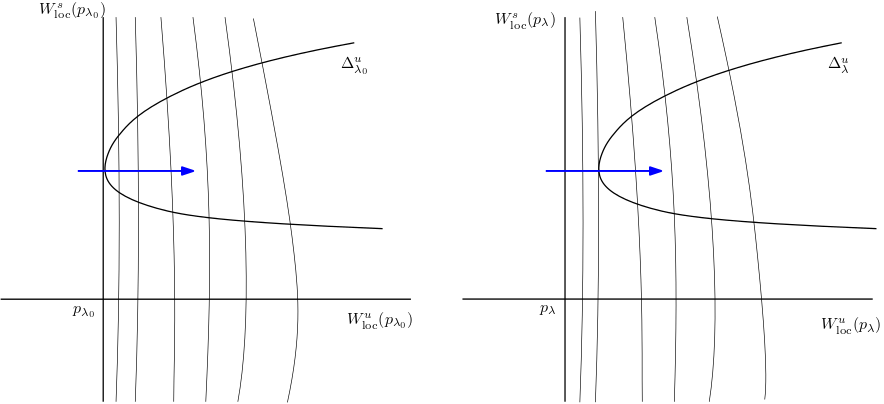
Figure 1. Creation of a secondary tangency

Now imagine a toy model for this situation where the stable manifolds of the horseshoe are just vertical lines and $\Delta^{u}_{\lambda}$ moves under a horizontal translation. In the holomorphic case one can easily imagine that the speed of motion of $\Delta^{u}_{\lambda}$ cannot vanish on a Cantor set of parameters (of course the reality is more complicated because the Cantor set of vertical lines moves with the parameter), so most tangencies should occur with positive speed. On the other hand, on this toy model it is unclear why, if we start with a tangency of high order, the order of the secondary tangencies would generically decrease. The point of Takens’ proof is to understand how the stable lamination of the horseshoe differs from a Cantor set of vertical lines, in order to lower the order of tangency. In this respect, a key notion is that of dynamical slope (see §4.2). The argument also requires delicate $C^{k}$ estimates for these vertical graphs, for large $k$ (see §4.1). The structure of the proof in the complex case is roughly the same as that of [36], but the technical details differ in many ways.

$\diamond$

As a consequence of Theorem A.1, all the phenomena associated to (one-dimensional) unfoldings of generic homoclinic tangencies appear in $\Lambda$. In particular by the recent work of Avila, Lyubich and Zhang [3], if $(f_{\lambda})$ is dissipative, $\Lambda$ contains Newhouse domains with robust homoclinic tangencies () and residually infinitely many sinks.

Another consequence is an extension and a strengthening of the “universality of the Mandelbrot set” phenomenon [25]: applying the quadratic renormalization theory of [29], it follows that in any one dimensional family $\Lambda$, baby Mandelbrot-looking sets (contrary to [25], we do not have to deal with Multibrot sets) appear in parameter space near any homoclinic tangency (). An interpretation of Theorem A.1 from the point of view of the analogy with one-dimensional dynamics is that active critical points of higher order do not exist for 2D diffeomorphisms (at least, under a non-resonance assumption).

For polynomial automorphisms of $\mathbb{C}^{2}$ (i.e. generalized complex Hénon maps), we can get rid of the non-resonance assumption, at the expense of potentially choosing another periodic point.

Theorem A.2.

Let $(f_{\lambda})_{\lambda\in\Lambda}$ be a holomorphic family of dissipative polynomial automorphisms of $\mathbb{C}^{2}$ of constant dynamical degree, parameterized by a complex manifold $\Lambda$. Assume that $f_{\lambda_{0}}$ admits a non-persistent homoclinic tangency. Then there exists $\lambda_{1}\in\Lambda$ arbitrary close to ${\lambda_{0}}$ such that $f_{\lambda_{1}}$ has a quadratic homoclinic tangency, unfolding with positive speed.

If $\Lambda$ is an open subset of the space of all generalized Hénon maps of a given degree, by Buzzard-Hruska-Illyashenko [11, Thm 1.4] there is no persistent resonance between the multipliers of a given periodic point, so Theorem A.1 applies directly. In particular no dissipativity assumption is required in this case. Let us also point out that a weaker version of this result was recently established by Araujo and Moreira in [1, Appendix], in which $f_{{\lambda_{0}}}$ is perturbed in an infinite dimensional space of entire mappings.

For families of polynomial diffeomorphisms of ${\mathbb{C}^{2}}$, it was shown in [17] that in the moderately dissipative regime $\left|\operatorname{Jac}(f)\right|<\deg(f)^{-2}$, homoclinic tangencies are dense in the bifurcation locus. Theorem A.2 thus implies that these homoclinic tangencies can be chosen to be quadratic with positive speed. Putting this together with the results of Avila-Lyubich-Zhang [3] we obtain:

Corollary A.3.

In any holomorphic family of moderately dissipative polynomial diffeomorphisms of $\mathbb{C}^{2}$ of a given degree, the bifurcation locus is the closure of its interior.

$\diamond$

The second main result of the paper is that for families of polynomial automorphisms of $\mathbb{C}^{2}$, persistent homoclinic tangencies also induce bifurcations.

Theorem B.1.

Let $(f_{\lambda})_{\lambda\in\Lambda}$ be a substantial family of polynomial automorphisms of $\mathbb{C}^{2}$ of constant dynamical degree, parameterized by a connected complex manifold $\Lambda$. Assume that there is a persistent homoclinic tangency associated to some saddle periodic point $p$ (with multipliers $u$ and $s$) such that the function $\lambda\mapsto\frac{\ln\left|u_{\lambda}\right|}{\ln\left|s_{\lambda}\right|}$ is non-constant. Then $(f_{\lambda})$ is not weakly $J^{\varstar}$-stable.

We refer to the Appendix for the meaning of the word “substantial” and the notion of weak $J^{\varstar}$-stability from [17], which is a weak form of structural stability on the Julia set. Here we content ourselves with pointing out that any dissipative family is substantial by definition, and that in this case the failure of weak $J^{\varstar}$-stability means that some saddle bifurcates to a sink (which implies the creation of new tangencies when $\left|\operatorname{Jac}(f)\right|<\deg(f)^{-2}$).

Since this result applies to any open subset of $\Lambda$, in the dissipative regime it follows from [17, Cor. 4.5] that Newhouse parameters, that is parameters displaying infinitely many sinks, are dense in $\Lambda$. Thus we obtain an alternate approach to the existence of such parameters which does not involve stable intersections of Cantor sets (see Yampolsky-Yang [37] for yet another approach, also using [17]).

It is quite simple to find examples of families satisfying the assumptions of Theorem B.1. For instance, it is classical that in the space of quadratic Hénon mappings with parameters $(a,c)\in\mathbb{C}^{\varstar}\times\mathbb{C}$, $f_{a,c}(z,w)=(aw+z^{2}+c,az)$, any (degenerate) parameter of the form $(0,c)$ where $c$ is strictly post-critically finite can be continued (in infinitely many ways) as a 1-parameter family of Hénon maps with a persistent tangency. It follows that $\left\{0\right\}\times\partial M$ (where $M$ is the Mandelbrot set) lies in the closure of the set of Newhouse parameters. In this case the assumption on the multipliers is easy to check because the Jacobian tends to zero along the parameter curve, so $s_{\lambda}\to 0$ while $u_{\lambda}$ is bounded away from 0 and infinity.

It is worth mentioning that two such curves (one homoclinic, one heteroclinic), landing at $(0,-2)$, were studied in detail by Bedford and Smillie in [5, 6], in the real setting. Along these families, the Julia set $J^{\varstar}$ is contained in $\mathbb{R}^{2}$, and no sink nor additional tangency is created as the Jacobian varies. This shows that Theorem B.1 is really about complex parameters.

To get further and prove the abundance of Newhouse parameters in the bifurcation locus, we have to check that the assumption on the multipliers is generically satisfied, up to a change of periodic point. This is similar in spirit to Theorem A.2, but also more delicate, and requires to work in the space of all polynomial automorphisms of a given degree.

Theorem B.2.

Let $\Lambda$ be an irreducible component of the space of generalized Hénon mappings of degree $d\geq 2$, and ${\lambda_{0}}\in\Lambda$ a parameter displaying a homoclinic tangency. Then in any neighborhood of ${\lambda_{0}}$ there is a hypersurface $\Lambda_{1}\subset\Lambda$ satisfying the assumptions of Theorem B.1. In particular if $\left|\operatorname{Jac}f_{\lambda_{0}}\right|\leq 1$, then ${\lambda_{0}}$ belongs to the closure of the set of Newhouse parameters.

To prove this, we have to rule out the unlikely phenomenon that as soon as a tangency is created near ${\lambda_{0}}$, then, along the corresponding hypersurface where this new tangency persists, the non-resonance condition of Theorem B.1 fails. Even if such a coincidence is hardly plausible, excluding it requires some non-trivial arguments. In particular we make heavy use the genericity results of [11].

Together with [17], Theorem B.2 gives an alternate argument for the following weak version of Corollary A.3.

Corollary B.3.

In the family of all moderately dissipative polynomial diffeomorphisms of $\mathbb{C}^{2}$ of a given degree, the bifurcation locus is contained in the closure of the set of Newhouse parameters.

This result is much weaker than Corollary A.3 because, instead of open sets where Newhouse parameters are residual, it only provides codimension 1 laminations. On the other hand, the proof is simpler since it does not resort to the results of [3]. We also note that another approach to the construction of Newhouse parameters was devised by Martens, Palmisano and Tao [24].

It is natural to wonder whether Theorem B.1 admits a local version as in Theorem A.1. The statement would be: in any family of diffeomorphisms of $\Omega\subset{\mathbb{C}^{2}}$ with a persistent homoclinic tangency, and such that $\frac{\ln\left|u_{\lambda}\right|}{\ln\left|s_{\lambda}\right|}$ is non-constant, non-persistent tangencies are created. There is a simple mechanism for this in the real setting, going back to the work of Gavrilov and Shil’nikov [20], which depends on the signs of certain auxiliary parameters (such restrictions are necessary in view of the above mentioned examples of Bedford-Smillie [6]).

To prove Theorem B.1, we take a different path and use the notion of moduli of stability, introduced by Palis [28] and further developed e.g. by Newhouse, Palis and Takens [27] and also by Buzzard [10] for diffeomorphisms of $\mathbb{C}^{2}$. In all these references, the authors start with a topological conjugacy between two diffeomorphisms in a neighborhood of an orbit of tangency to deduce a differentiable rigidity of the multipliers ([28] further relies on plane topology considerations). We show that this notion can be adapted to the context of the weak $J^{\varstar}$-stability theory of [17], which does not yield topological conjugacies. As observed above, the results of [5, 6] show that it is essential here to work in the complex setting. A key idea is that the holomorphic motion of saddle periodic points admits a natural extension to stable and unstable manifolds, which satisfy good distortion properties. This provides a reasonably simple proof of Theorem B.1, which takes advantage of the global geometric structure of complex Hénon mappings and showcases the techniques of [17].

Note that it is actually also possible to adapt the Gavrilov-Shil’nikov mechanism to the complex setting, at least for quadratic tangencies. The details (which are a bit technical) will appear elsewhere.

Remark 1.1.

Theorems B.1 and B.2 bear some similarity with recent work of Gauthier, Taflin and Vigny [19], where “higher bifurcations” are studied in spaces of regular endomorphisms of $\mathbb{P}^{k}(\mathbb{C})$ (see also [2], as well as [16] for a brief account on this topic). These theorems can actually be interpreted from the perspective of higher bifurcations (at least in the moderately dissipative regime): indeed the bifurcation locus has some codimension 1 structure given by the hypersurfaces of persistent homoclinic tangencies, and inside these hypersurfaces Theorem B.1 can recursively be used to construct new tangencies. One might expect that the analogue of Theorem B.2 holds recursively, so that if $\Lambda$ is a component of the space of polynomial automorphisms of given degree, then on a dense subset of the bifurcation locus there should be $\dim(\Lambda)$ “independent” tangencies.

Outline

We start in Section 2 with some geometric preliminaries on submanifolds of the bidisk. In Section 3, we apply basic ideas from local complex geometry to define and give a neat treatment of the notions of order, speed exponent and multiplicity of a non-persistent tangency. Theorems A.1 and A.2 are proven in Section 4. As explained above, the most delicate point is to produce quadratic tangencies, which requires $C^{k}$ graph transform estimates (§4.1) and to develop a notion of dynamical slope (§4.2). In Section 5 we study persistent tangencies and prove Theorems B.1 and B.2. In the Appendix we briefly review the notion of weak stability from [17].

Notation and conventions

The unit disk in $\mathbb{C}$ is denoted by $\mathbb{D}$ and we let $\mathbb{B}=\mathbb{D}\times\mathbb{D}$. The letter $C$ stands for a “constant” which may change from line to line, independently of some asymptotic quantity that should be clear from the context. We make heavy use of the following notation: we write $a\lesssim b$ if $\left|a\right|\leq C\left|b\right|$, $a\asymp b$ if $a\lesssim b\lesssim a$, and $a\cong b$ if $a\sim cb$ for some $c\in\mathbb{C}^{\varstar}$. We denote by $\left\|\cdot\right\|_{\Omega}$ the uniform norm in a domain $\Omega$. The eigenvalues at a saddle periodic point will be generally denoted by $u$ and $s$ (or $u_{\lambda}$ and $s_{\lambda}$ in the presence of a parameter), where it is understood that $\left|u\right|>1$ and $\left|s\right|<1$.

Acknowledgments

Thanks to Artur Avila, Misha Lyubich and Zhiyuan Zhang for their work on the complex Newhouse phenomenon which prompted me to finally tackle this project, to Sébastien Biebler for many discussions on this topic, and to Marc Chaperon for his help with Sternberg’s theory.

2. Preliminary geometric lemmas

2.1. Transversality lemma

The following basic lemma is very useful.

Lemma 2.1 (see [4, Lem. 6.4]).

Let $\Delta$ and $\Delta^{\prime}$ be two holomorphic disks with an isolated tangency of order $h$ at $p$. Then if $\Delta^{\prime\prime}$ is a holomorphic disk disjoint from $\Delta$ and sufficiently $C^{1}$ close to it, it intersects $\Delta^{\prime}$ transversally in $h+1$ points close to $p$.

Observe that this result does not hold in higher dimension, due to the possibility of non-proper intersections: this is precisely the reason why Theorem A.1 is non-trivial (cf. the formalism of §3.2). An explicit example where the higher dimensional version of this lemma fails is obtained by lifting the basic toy model from the Introduction to the projectivized tangent bundle.

2.2. Horizontal and vertical varieties in $\mathbb{B}$

Recall that $\mathbb{B}$ is the unit bidisk. We let $\partial^{h}\mathbb{B}=\mathbb{D}\times\partial\mathbb{D}$ (resp. $\partial^{v}\mathbb{B}=\partial\mathbb{D}\times\mathbb{D}$) be its horizontal (resp. vertical) boundary. A subvariety $V$ in some neighborhood of $\overline{\mathbb{B}}$ is horizontal (resp. vertical) in $\mathbb{B}$ if $V\cap\partial^{h}\mathbb{B}=\emptyset$ (resp. $V\cap\partial^{v}\mathbb{B}=\emptyset$). A horizontal (resp. vertical) subvariety is a branched cover over the unit disk for the first (resp. second) projection so it has a degree, which is the degree of this cover. If $V_{1}$ (resp. $V_{2}$ is a horizontal (resp. vertical) variety of degree $d_{1}$ (resp. $d_{2}$), then $V_{1}$ and $V_{2}$ intersect in $d_{1}d_{2}$ points, counting multiplicity (see e.g. [14] for more details on these notions).

Lemma 2.2.

Let $\Delta$ be a horizontal submanifold in $\mathbb{B}$ of degree $d$ which is a union of holomorphic disks, and $(W_{i})_{i\in I}$ an arbitrary collection of disjoint vertical disks. Then the total number of tangencies between $\Delta$ and the $W_{i}$, counting multiplicities, is bounded by $d-1$

Proof.

The union of the $W_{i}$ and $\partial^{v}\mathbb{B}=\bigcup_{\zeta\in\partial\mathbb{D}}\left\{\zeta\right\}\times\mathbb{D}$ is a lamination by vertical graphs. By Lemma 2.1, by slightly perturbing the radius of the bidisk, we may assume that $\Delta$ is transverse to $\partial^{v}\mathbb{B}$. If we fix a horizontal slice, for instance $L:=\mathbb{D}\times\left\{0\right\}$, which we identify to $\mathbb{D}$, this lamination can be viewed as a holomorphic motion of $\partial\mathbb{D}\cup(\bigcup W_{i}\cap L)$, which can be extended to a motion of $\overline{\mathbb{D}}$ by Slodkowski’s theorem [32]. Note that since the motion is the identity on $\partial\mathbb{D}$, it must preserve $\mathbb{D}$. The corresponding lamination of $\mathbb{B}$ by vertical graphs fills up the whole bidisk.

Let $\pi:\mathbb{B}\to\mathbb{D}$ be the projection along this lamination. Since $\Delta$ intersects any vertical graph in $d$ points, $\pi\arrowvert_{\Delta}:\Delta\to\mathbb{D}$ is a branched cover of degree $d$. If we can show that this branched cover satisfies the Riemann-Hurwitz formula, then the total number of tangencies, counting multiplicity, is at most $(d-1)$, and the lemma follows. To prove this fact, we first note that by Lemma 2.1, only finitely many $W_{i}$ are tangent to $\Delta$. They correspond to the critical points of $\pi\arrowvert_{\Delta}$. Then we argue as in the usual proof of the Riemann-Hurwitz formula, by pulling back a triangulation of the base whose vertex set contains the critical values, and computing the Euler characteristic of the pulled-back triangulation (which is equal to the number of components of $\Delta$). The only delicate point is to show that at the critical points, $\pi$ behaves topologically like a holomorphic map: this follows from the fact that near such a point, $\pi$ is of the form $u\circ k$, where $u$ is a holomorphic map and $k$ is a quasiconformal homemorphism (see [15, p. 590]). ∎

Lemma 2.3.

Let $\Delta$ be a horizontal submanifold in $\mathbb{B}$ of degree $d$ which is a union of holomorphic disks. Assume that there is a vertical graph $W$ in $\mathbb{B}$ which is tangent to order $d-1$ to $\Delta$. Then $\Delta$ has $d$ vertical tangencies in $\mathbb{B}$

Proof.

Fix $R<1$ such that $W$ is vertical in $R\mathbb{D}\times\mathbb{D}$. Since the number of vertical tangencies of $\Delta$ is finite, there exists $R\leq R^{\prime}\leq 1$ such that $\Delta$ is transverse to $\partial(R^{\prime}\mathbb{D})\times\mathbb{D}$. Without loss of generality we replace $\mathbb{D}$ by $R^{\prime}\mathbb{D}$. Each component of $\Delta$ is a horizontal submanifold intersecting $W$. Since $W\cap\Delta$ admits $d$ points counting multiplicities, we infer that $W\cap\Delta$ is reduced to the tangency point, of multiplicity $d$. Hence $\Delta$ is made of a single component, and the result follows from the Riemann-Hurwitz formula applied to the first projection. ∎

2.3. Tangency creation lemma

Lemma 2.4 (see [17, Prop. 8.1]).

Let $(\Delta_{\lambda})_{\lambda\in\Lambda}$ be a holomorphic family of horizontal submanifolds of degree $d$ in $\mathbb{B}$, with $\Lambda\simeq\mathbb{D}$. Assume that for $\lambda$ close to $\partial\Lambda$, $\Delta_{\lambda}$ is a union of horizontal graphs, and that this property does not hold for some $\lambda_{0}\in\Lambda$.

Let $(W_{\lambda})_{\lambda\in\Lambda}$ be a holomorphic family of vertical graphs in $\mathbb{B}$. Then there exists a non-empty finite set of parameters such that $\Delta_{\lambda}$ and $W_{\lambda}$ are tangent.

The finiteness of the set of tangency parameters was not stated in [17, Prop. 8.1] but it is explicitly mentioned in its proof (see also [35] for a counting of the number of tangency parameters).

3. Complex geometry of homoclinic tangencies

3.1. Conventions

Let $\Omega\subset\mathbb{C}^{2}$ be an open set and $f:\Omega\to f(\Omega)\subset\mathbb{C}^{2}$ be a diffeomorphism with a saddle fixed point $p$, with local stable and unstable manifolds $W^{s/u}_{\mathrm{loc}}(p)$ (we use the notation $W^{s}_{\mathrm{loc}}(p)$ for the component of $W^{s}(p)\cap\Omega$ containing $p$). In such a semi-local setting, the global stable manifold $W^{s}(p)$ is the set of points $x\in\Omega$ such that $f^{n}(x)$ belongs to $\Omega$ for every $n\geq 0$ and eventually falls into $W^{s}_{\mathrm{loc}}(p)$, and likewise for $W^{u}(p)$.

Assume that there is a tangency between $W^{s}(p)$ and $W^{u}(p)$ at $\tau$. We will generally use the following normalization: upon iteration one may assume that $\tau\in W^{s}_{\mathrm{loc}}(p)$; we pick local coordinates $(x,y)\in\mathbb{B}$ such that $p=0$, $f(x,y)=(ux,sy)+{\mathrm{h.o.t.}}$ and $W^{s}_{\mathrm{loc}}(p)=\left\{x=0\right\}$, so that $\tau=(0,y_{0})$. The branch of $W^{u}(p)$ tangent to $W^{s}_{\mathrm{loc}}(p)$ at $\tau$, denoted $\Delta^{u}$, is locally of the form $x=\varphi(y)$, where $\varphi$ a holomorphic function defined in a neighborhood of $y_{0}$, with $\varphi(y_{0})=\varphi^{\prime}(y_{0})=0$ (see Figure 1). We say that the tangency is of order $h$ if the order of contact –which must be finite– equals $h+1$, that is $\varphi(y)\cong(y-y_{0})^{h+1}$ as $y\to y_{0}$ (recall that this means $\varphi(y)\sim c(y-y_{0})^{h+1}$ for some $c\neq 0$). So a quadratic tangency is a tangency of order 1.

Now let $f$ depend holomorphically on a parameter $\lambda\in\Lambda$, so that all the above defined objects depend holomorphically on $\lambda$, and are denoted by $f_{\lambda}$, $W^{s/u}_{\lambda}$, etc. The parameter space $\Lambda$ is typically the unit disk, but for clarity we keep the notation $\Lambda$. The tangency parameter is denoted by $\lambda_{0}$, and without loss of generality we assume $\lambda_{0}=0$. Our study is local near $\lambda_{0}$, so we may reduce $\Lambda$ without further notice. Again we choose local coordinates $(x,y)$ such that $p_{\lambda}=(0,0)$ and $W^{s}_{\mathrm{loc}}(p_{\lambda})=\left\{x=0\right\}$.

The tangency is non-persistent if for $\lambda\neq\lambda_{0}$ close to $\lambda_{0}$, $\Delta^{u}_{\lambda}$ is not tangent to $W^{s}_{\lambda}(p_{\lambda})$, hence in a holomorphic setting it must intersect it transversally. It is not so easy in the smooth category to define a formal notion of “speed of motion” for the tangency: first, when $\lambda\neq\lambda_{0}$, there is no homoclinic tangency to work with. A common idea is to consider vertical tangencies of $\Delta^{u}_{\lambda}$ as a kind of “virtual” tangency, and look at the speed of motion of these tangencies (). Next, in the complex setting, when $h>1$ the tangency usually splits into $h$ vertical tangencies, which may or may not be followed holomorphically. The good news is that there is still a unequivocal notion of a generically unfolding or “positive speed” tangency, as we explain in §3.3 below.

Note that for persistent tangencies, it may be the case that for $\lambda={\lambda_{0}}$ the tangency is of order $h$, while for $\lambda\neq{\lambda_{0}}$ it splits off into a persistent tangency of order $h^{\prime}<h$ together with $h-h^{\prime}$ vertical tangencies.

3.2. Lifting to the projectivized tangent bundle

The following viewpoint was developed in [17, §9.1]. Consider a family of two holomorphically varying smooth complex submanifolds $(V_{\lambda})_{\lambda\in\Lambda}$ and $(W_{\lambda})_{\lambda\in\Lambda}$ in $\mathbb{B}$, with $\Lambda=\mathbb{D}$. For every $\lambda$, we denote by $\mathbb{P}TV_{\lambda}$ (resp. $\mathbb{P}TW_{\lambda}$) the lift of $V_{\lambda}$ (resp. $W_{\lambda}$) to the projectivized tangent bundle $\mathbb{P}T\mathbb{B}\simeq\mathbb{B}\times{\mathbb{P}^{1}}$. Finally, we define a 2-dimensional subvariety $\widehat{\mathbb{P}TV}$ of $\Lambda\times\mathbb{B}\times{\mathbb{P}^{1}}$ by putting together the $\mathbb{P}TV_{\lambda}$, that is $\widehat{\mathbb{P}TV}\cap\left\{\lambda\right\}\times\mathbb{B}\times{\mathbb{P}^{1}}=\mathbb{P}TV_{\lambda}$, and likewise for $\widehat{\mathbb{P}TW}$ A non-persistent tangency between $V_{0}$ and $W_{0}$ then corresponds to an isolated intersection of $\widehat{\mathbb{P}TV}$ and $\widehat{\mathbb{P}TW}$. Let us denote by $\widehat{0}$ the corresponding intersection point Since in this case

$$\operatorname{codim}_{\widehat{0}}\left(\widehat{\mathbb{P}TV}\cap\widehat{\mathbb{P}TW}\right)=\operatorname{codim}_{\widehat{0}}\left(\widehat{\mathbb{P}TV}\right)+\operatorname{codim}_{\widehat{0}}\left(\widehat{\mathbb{P}TW}\right),$$

this intersection is proper so it has nice properties, in particular the intersection multiplicity $\operatorname{mult}_{\widehat{0}}\left(\widehat{\mathbb{P}TV},\widehat{\mathbb{P}TW}\right)$ is well-defined (see [12, §12]). By definition this number is the multiplicity of the tangency.

Lemma 3.1.

With notation as in §3.1, $\widehat{\mathbb{P}TW^{s}}$ and $\widehat{\mathbb{P}T\Delta^{u}}$ are smooth, and

(1) $$\operatorname{mult}_{\widehat{0}}\left(\widehat{\mathbb{P}TW^{s}},\widehat{\mathbb{P}T\Delta^{u}}\right)\geq h,$$

where $h$ is the order of tangency.

Proof.

The multiplicity in (1) can be computed by intersecting two curves, as follows. Recall that we fixed local coordinates such that $W^{s}_{\mathrm{loc}}(p_{\lambda})=\left\{x=0\right\}$, and $\Delta^{u}_{\lambda}=\left\{x=\varphi_{\lambda}(y)\right\}$. Write $y=y_{0}+t$ and $\varphi_{y_{0}}(\lambda,t):=\varphi(\lambda,y_{0}+t)$ so that near the point of tangency, $\Delta^{u}_{\lambda}$ is parameterized by $(t,\varphi_{y_{0}}(\lambda,t))$, whose tangent vector is $(1,\dot{\varphi}_{y_{0}}(\lambda,t))$, where the dot denotes derivation with respect to the $t$-variable. In $\mathbb{P}T\mathbb{C}^{2}\simeq\mathbb{P}^{1}$, denote by $w$ the coordinate in the affine chart containing $[1,0]$. Thus we have local coordinates $(\lambda,t,x,w)$ in $\Lambda\times\mathbb{B}\times{\mathbb{P}^{1}}$, in which we have the equations

$$\begin{cases}x=\varphi_{y_{0}}(\lambda,t)\\ w=\dot{\varphi}_{y_{0}}(\lambda,t)\end{cases}\text{ for }\widehat{\mathbb{P}T\Delta^{u}}\ \text{ and }\begin{cases}x=0\\ w=0\end{cases}\text{ for }\widehat{\mathbb{P}TW^{s}},$$

and it follows that both varieties are smooth and $\operatorname{mult}_{\hat{0}}\left(\widehat{\mathbb{P}TW^{s}},\widehat{\mathbb{P}T\Delta^{u}}\right)$ is equal to the intersection multiplicity of the curves $\mathcal{C}:=\left\{\varphi_{y_{0}}(\lambda,t)=0\right\}$ and $\dot{\mathcal{C}}:=\left\{\dot{\varphi}_{y_{0}}(\lambda,t)=0\right\}$, which admit an isolated intersection at $(0,0)$. This is clear if we think of the multiplicity as the number of intersections of generic local translations of $\widehat{\mathbb{P}T\Delta^{u}}$ and $\widehat{\mathbb{P}TW^{s}}$ (see [12, §12]). Recall that the classical definition of multiplicity of the intersection of two curves is $\operatorname{mult}_{0}(\mathcal{C},\dot{\mathcal{C}})=\dim\mathcal{O}({\mathbb{C}^{2}},0)/\langle\varphi_{y_{0}},\dot{\varphi}_{y_{0}}\rangle$. In the situation at hand we have

(2) $$\begin{cases}\varphi_{y_{0}}(\lambda,t)=ct^{h+1}+O({t^{h+2}})+O\left(\lambda\right)\\ \dot{\varphi}_{y_{0}}(\lambda,t)=cht^{h}+O({t^{h+1}})+O\left(\lambda\right)\end{cases}$$

hence $\mathcal{O}({\mathbb{C}^{2}},0)/\langle\varphi_{y_{0}},\dot{\varphi}_{y_{0}}\rangle$ contains all monomials $1,t,\ldots,t^{h-1}$ and its dimension is at least $h$. ∎

3.3. Speed of motion

We now explain how the multiplicity defined above takes into account both the order and the speed of motion of the tangency. Recall from the proof of Lemma 3.1 that the multiplicity of tangency equals $\operatorname{mult}_{0}(\mathcal{C},\dot{\mathcal{C}})$, where $\mathcal{C}=\left\{\varphi_{y_{0}}(\lambda,t)=0\right\}$ and $\dot{\mathcal{C}}=\left\{\dot{\varphi}_{y_{0}}(\lambda,t)=0\right\}$.

For simplicity , let us first assume that $\dot{\mathcal{C}}$ is irreducible at $(0,0)$. For a fixed small $\lambda\neq 0$, the equation $\dot{\varphi}_{y_{0}}(\lambda,t)=0$ admits $h$ solutions (that is, there are $h$ vertical tangencies) so $\dot{\mathcal{C}}$ can be parameterized by a Puiseux series in $t^{1/h}$. In usual complex geometric language, there is a coordinate $\mu$ on the normalization of ${\dot{\mathcal{C}}}$ such that the expression of the composition of the normalization map and the first projection $(\lambda,t)\mapsto\lambda$ is $\mu\mapsto\mu^{h}$, hence $\dot{\mathcal{C}}$ admits a local (injective) parameterization of the form $\mu\mapsto(\mu^{h},\theta(\mu))$, for some holomorphic function $\theta$ with $\theta(0)=0$. Writing

(3) $$\varphi_{y_{0}}(\lambda,t)=ct^{h+1}+O({t^{h+2}})+\lambda\psi(\lambda,t)$$

and substituting, we infer that

(4) $$\varphi_{y_{0}}(\mu^{h},\theta(\mu))=c\theta(\mu)^{h+1}+O({\theta(\mu)^{h+2}})+\mu^{h}\psi(\mu^{h},\theta(\mu)),$$

and the multiplicity $m$ of tangency is the order of vanishing of this expression at $\mu=0$ (since the tangency is non-persistent, $\mu\mapsto\varphi_{y_{0}}(\mu^{h},\theta(\mu))$ has an isolated zero at the origin). This yields another proof that $m\geq h$, with equality if and only if $\psi(0,0)\neq 0$, that is,

(5) $$\varphi_{y_{0}}(\lambda,t)=ct^{h+1}+d\lambda+{\mathrm{h.o.t.}},\text{ with }d=\psi(0,0).$$

In the language of Puiseux series, this reads

(6) $$\varphi_{y_{0}}(\lambda,\theta(\lambda^{1/h}))=c\theta(\lambda^{1/h})^{h+1}+O({\theta(\lambda^{1/h})^{h+2}})+\lambda\psi(\lambda,\theta(\lambda^{1/h})).$$

The speed of motion $\sigma$ of the vertical tangencies is characterized by the exponent of $\lambda$ in $\varphi_{y_{0}}(\lambda,\theta(\lambda^{1/h}))$, that is, $\varphi_{y_{0}}(\lambda,\theta(\lambda^{1/h}))\cong\lambda^{\sigma}$, where $\sigma=m/h\geq 1$ (which is typically not an integer), and we see that non-vanishing speed of motion at $\lambda=0$ (i.e. non-degenerate unfolding) corresponds to $m=h$, as expected from (5). Note that for quadratic tangencies ($h=1$), this simply means that $\widehat{\mathbb{P}TW^{s}}$ and $\widehat{\mathbb{P}T\Delta^{u}}$ are transverse at $\widehat{0}$.

Beware, however, that non-vanishing speed of motion (i.e. $\sigma=1$) does not imply that the vertical tangencies can be followed holomorphically, as shown for instance by the example $\varphi_{y_{0}}(\lambda,t)=t^{h+1}+\lambda(1+t)$, for which the abscissae of vertical tangencies are given by $\lambda+c\lambda^{1+1/h}$ for some explicit $c$.

In the general case where $\dot{\mathcal{C}}$ is reducible, write $\dot{\varphi}_{y_{0}}(\lambda,t)\cong\prod_{j=1}^{q}\xi_{j}(\lambda,t)$ (up to some invertible element of $\mathcal{O}({\mathbb{C}^{2}},0)$), where $\xi_{j}(0,t)=t^{h_{j}}+{\mathrm{h.o.t.}}$, and $\sum_{j}h_{j}=h$. Each branch $\dot{\mathcal{C}}_{j}$ is injectively parameterized by $\mu\mapsto(\mu^{h_{j}},\theta_{j}(\mu))$, $\theta_{j}(0)=0$, and substituting this expression in $\varphi_{y_{0}}$ as in (4) gives

(7) $$\varphi_{y_{0}}(\mu^{h_{j}},\theta_{j}(\mu))=c\theta_{j}(\mu)^{h+1}+O({\theta_{j}(\mu)^{h+2}})+\mu^{h_{j}}\psi(\mu^{h_{j}},\theta_{j}(\mu)).$$

This shows that $m_{j}\geq h_{j}$, where $m_{j}=\operatorname{mult}_{0}(\mathcal{C},\dot{\mathcal{C}}_{j})$, with equality if and only if $\psi(0,0)\neq 0$ (this condition does not depend on $j$), and $\sigma_{j}:=m_{j}/h_{j}$ is the speed exponent of the block of $h_{j}$ tangencies corresponding to $\dot{\mathcal{C}}_{j}$. By the additivity of multiplicity, we conclude that $m=\sum_{j=1}^{q}h_{j}\sigma_{j}$. Combining this relation with $\sum_{j}h_{j}=h$, shows that $m=h$ if and only if $\sigma_{j}=1$ for every $j$, so again the equality $m=h$ characterizes a non-degenerate unfolding.

3.4. Secondary intersections

The following result is specific to complex diffeomorphisms. Note that for polynomial automorphisms of $\mathbb{C}^{2}$ it also follows from global arguments (see [4, §9]).

Proposition 3.2.

If $f:\Omega\to{\mathbb{C}^{2}}$ is a diffeomorphism with a homoclinic tangency associated to $p$, then there are also transverse homoclinic intersections between $W^{s}(p)$ and $W^{u}(p)$.

To get an intuition of what is going on, let us explain the argument (which is classical) in the oversimplified case where the dynamics in linearizable at $p$. In this case we can simply write $f(x,y)=(ux,sy)$. With notation as in §3.1 we have a branch $\Delta^{u}$ of $W^{u}(p)$ tangent to $W_{\mathrm{loc}}^{s}(p)$ at $(0,y_{0})$, with equation $x=\varphi(y)\cong(y-y_{0})^{h+1}$. Pulling back this pair of curves by for some iterate $f^{k}$, we get a branch $\Delta^{s}\subset W^{s}(p)$ tangent to $W^{u}_{\mathrm{loc}}(p)$ at $(x_{0},0)$, with equation $y=\psi(x)\cong(x-x_{0})^{h+1}$. If $(x,y)\in\Delta^{u}$ with $\left|x\right|\ll 1$, then a tangent vector to $\Delta^{u}$ at $(x,y)$ is $v\asymp(x^{h/(h+1)},1)$, whose slope is $\asymp x^{-h/(h+1)}$. Likewise, if $(x,y)\in\Delta^{s}$ with $\left|y\right|\ll 1$, then the slope of $\Delta^{s}$ at $(x,y)$ is $\asymp y^{h/(h+1)}$. Now let us assume for the moment that some version of the argument principle guarantees that $f^{n}(\Delta^{u})$ intersects $\Delta^{s}$ for large $n$, so there exists $(x_{0},y_{0})\in\Delta^{u}$ such that $(x_{n},y_{n})=(u^{n}x_{0},s^{n}y_{0})\in\Delta^{s}$. Then with notation as above, $v\asymp(u^{-nh/(h+1)},1)$ so its image under $df^{n}$ is $\asymp(u^{n}u^{-nh/(h+1)},s^{n})$ whose slope is $s^{n}u^{-nh/(h+1)}$. On the other hand the slope of $T\Delta^{s}$ at $(x_{n},y_{n})$ is $\asymp s^{nh/(h+1)}\gg s^{n}u^{-nh/(h+1)}$ so $f^{n}\Delta^{u}$ is transverse to $\Delta^{s}$. Making this argument rigorous in the non-linearizable case is quite technical, and it is remarkable that in the complex setting all these estimates can be replaced by geometric analysis considerations.

Proof.

We keep notation as above, and use the formalism of horizontal/vertical objects and crossed mappings from [23] (or Hénon-like mappings of degree 1 in the language of [14]). Consider a thin vertical bidisk around $W^{s}(p)$ of the form $D(0,\delta)\times\mathbb{D}$. Then for small enough $\delta$, $\Delta^{u}$ is a horizontal disk of degree $h+1$ in $D(0,\delta)\times\mathbb{D}$. Likewise, reducing $\delta$ if necessary, $\Delta^{s}$ is a vertical disk of degree $h+1$ in $\mathbb{D}\times D(0,\delta)$. By the Inclination lemma, for large $n$, $f^{n}$ defines a crossed mapping of degree 1 from $D(0,\delta)\times\mathbb{D}$ to $\mathbb{D}\times D(0,\delta)$. Therefore the graph transform $\mathcal{L}^{n}\Delta^{u}$ of $\Delta^{u}$ (that is, its image under the crossed mapping) is a horizontal disk of degree $h+1$ in $\mathbb{D}\times D(0,\delta)$, so it intersects $\Delta^{s}$ in $(h+1)^{2}$ points, counting multiplicities. We claim that for large $n$ all these intersections are transverse. Indeed when $\delta$ is small enough, $\Delta^{s}\cap(\mathbb{D}\times D(0,\delta))$ is contained in $D(x_{0},r)\times D(0,\delta)$, where $r<\left|x_{0}\right|/2$. Now, since $\mathcal{L}^{n}\Delta^{u}$ admits a tangency of order $h$ with $W^{s}_{\mathrm{loc}}(p)$ and since by the maximum principle it is a topological disk, by the Riemann-Hurwitz formula it admits no other vertical tangency (see also Lemma 2.2). So $\mathcal{L}^{n}\Delta^{u}\cap(D(x_{0},r)\times D(0,\delta))$ is the union of $h+1$ horizontal graphs disjoint from $D(x_{0},r)\times\left\{0\right\}$, and close to it. Then by Lemma 2.1 these graphs must be transverse to $\Delta^{s}$, and we are done. ∎

Remark 3.3.

Since there are homoclinic intersections, $W^{u}(p)$ must accumulate itself. In particular there are disks contained in $W^{u}(p)$ arbitrary $C^{1}$ close to $\Delta^{u}$. Applying Lemma 2.1 again then produces transverse intersections between these disks and $W^{s}_{\mathrm{loc}}(p)$, such that the angle between the tangent spaces at the intersection is arbitrary small. This observation will be crucial later.

3.5. Comments on higher dimensional families

Still working under the conventions of §3.1, assume in this paragraph only that $k:=\dim(\Lambda)>1$. Let $\mathcal{T}\subset\Lambda$ be the locus of tangency between $W^{s}_{\lambda}$ and $\Delta^{u}_{\lambda}$. Our purpose is to study the basic properties of $\mathcal{T}$.

Arguing exactly as in Lemma 3.1, we see that $\widehat{\mathbb{P}TW^{s}}$ and $\widehat{\mathbb{P}T\Delta^{u}}$ are smooth and of codimension 2 in $\Lambda\times\mathbb{B}\times\mathbb{P}^{1}$, so [12, §3.5] $\dim(\widehat{\mathbb{P}TW^{s}}\cap\widehat{\mathbb{P}T\Delta^{u}})\geq 2(k+1)-(k+3)=k-1$. It is clear that the natural projection $\pi_{\Lambda}:\Lambda\times\mathbb{B}\times\mathbb{P}^{1}\to\Lambda$ is finite and locally proper in restriction to $\widehat{\mathbb{P}TW^{s}}\cap\widehat{\mathbb{P}T\Delta^{u}}$, so it preserves dimensions [12, §3.3] and $\mathcal{T}$ is an analytic subset of dimension at least $k-1$. Since the tangency is not persistent, $\dim(\mathcal{T})<k$, and we conclude that $\dim(\mathcal{T})=k-1$, that is, $\mathcal{T}$ is an analytic hypersurface.

Slightly abusing terminology, we say that the homoclinic tangency has positive speed if there exists a smooth 1-dimensional subfamily $\Lambda_{1}\ni\lambda_{0}$ along which this property holds. Then, in the 4-dimensional subspace $\Lambda_{1}\times\mathbb{B}\times{\mathbb{P}^{1}}$, the intersection $\widehat{\mathbb{P}TW^{s}}\cap\widehat{\mathbb{P}T\Delta^{u}}$ (which is reduced to a point) is transverse. Counting dimensions in the tangent space, it is easy to see that it implies the corresponding transversality in $\Lambda\times\mathbb{B}\times{\mathbb{P}^{1}}$. And since the fibers of the projections $\pi_{\Lambda}$ and $\pi_{\Lambda_{1}}$ coincide, we also deduce that in $\Lambda\times\mathbb{B}\times{\mathbb{P}^{1}}$, $\widehat{\mathbb{P}TW^{s}}\cap\widehat{\mathbb{P}T\Delta^{u}}$ is transverse to $\pi_{\Lambda}^{-1}(\left\{{\lambda_{0}}\right\})$. This implies that if the unfolding has positive speed, $\mathcal{T}$ is smooth at ${\lambda_{0}}$.

4. Unfolding degenerate tangencies

4.1. Linearization and graph transform estimates

As in [36, §3], a key technical fact in the argument of Theorem A.1 is that in the graph transform, higher derivatives converge faster and faster to zero. This is obvious for the linear map $f(x,y)=(ux,sy)$: indeed the forward iterate of the graph $y=\gamma(x)$ is $y=\mathcal{L}^{n}\gamma(x)$, with $\mathcal{L}^{n}\gamma:x\mapsto s^{n}\gamma(x/u^{n})$ so $\|(\mathcal{L}^{n}\gamma)^{(\ell)}\|=O((su^{-\ell})^{n})$. It is unclear to us whether such an estimate holds in general, and to achieve this, as in [36] we use $C^{\ell}$ linearization, which imposes some conditions on the multipliers $u$ and $s$. Even if this belongs to real dynamics, we want to salvage as much complex geometry as possible –in particular we need to be able to talk about the complex multipliers $u$ and $s$, and not only their moduli, which is important in the parameter exclusion in §4.3– so the presentation is different from that of Takens (and since this matter is quite delicate we actually give more details). In particular we will not switch between different coordinate systems in the proof of the main theorem, and always stay in holomorphic coordinates, which in our opinion makes the argument neater.

An important remark is that to achieve $\|(\mathcal{L}^{n}\gamma)^{(j)}\|=O((su^{-j})^{n})$ for all $j\leq\ell$ it is not enough to merely know the existence of a system of $C^{\ell}$ linearizing coordinates: we also need this coordinate system to be flat up to a high order $K=K(\ell)$ along the separatrices, to prevent lower derivatives of the chart to spoil the estimate $\|(\mathcal{L}^{n}\gamma)^{(j)}\|=O((su^{-j})^{n})$. Finally, we need some uniformity of these estimates with respect to parameters.

4.1.1. Normal form

The first stage is to put $f$ in an appropriate normal form, under a non-resonance condition. Denote by $\mathfrak{M}$ the maximal ideal of the local ring of germs of holomorphic functions in $({\mathbb{C}^{2}},0)$, that is, the ideal of functions vanishing at the origin. Recall that if $f(x,y)=(ux,sy)+{\mathrm{h.o.t.}}$, a resonance of order $k$ is a relation of the form $u=u^{a}s^{b}$ or $s=u^{a}s^{b}$, where $a$ and $b$ are positive integers with $a+b=k$. When $\left|s\right|<1<\left|u\right|$, this can be rewritten as $u^{a}s^{b}=1$, with $a+b=k-1$. It is well-known that resonances are obstructions to holomorphic (and even formal) linearization. More precisely, a resonance of the form $u=u^{a}s^{b}$ (resp. $s=u^{a}s^{b}$) prevents from killing the term $x^{a}y^{b}$ in the first (resp. second) component of $f$. Conversely, if $f$ has no resonance up to order $k$, a holomorphic (actually polynomial) change of coordinates brings $f$ to the form

(8) $$f(x,y)=(ux+g_{1}(x,y),sy+g_{2}(x,y)),\text{ with }g_{1},g_{2}\in\mathfrak{M}^{k+1}.$$

The following more precise normal form is presumably known to some experts. We include the proof for completeness.

Proposition 4.1.

Let $f\in\operatorname{Diff}({\mathbb{C}^{2}},0)$ with a saddle fixed point at the origin, with eigenvalues $u$ and $s$. If there is no resonance up to order $k+1$, $f$ can be brought to the form

($$\star_{k} f(x,y)=(ux(1+yg_{1}(x,y)),sy(1+xg_{2}(x,y))),\text{ with }g_{1},g_{2}\in\mathfrak{M}^{k}.$$)

by a holomorphic change of coordinates.

Proof.

We review the proof of the existence of the local stable and unstable manifolds, by checking that the corresponding change of coordinates are sufficiently tangent to identity at the origin. Let us first deal with the local unstable manifold. We follow Sternberg [33, Thms 7 to 9, §9]. To stick with the notation of [33, p. 823], we put $T=f^{-1}$. Thanks to the non-resonance assumption, we can assume that

(9) $$T(x,y)=(u^{-1}x+\tilde{g}_{1}(x,y),s^{-1}y+\tilde{g}_{2}(x,y)),\text{ with }\tilde{g}_{1},\tilde{g}_{2}\in\mathfrak{M}^{k+2}.$$

We first look for a change of coordinates $R:(x,y)\mapsto(x,y-\phi(x))$ with $\phi^{\prime}(0)=0$ such that $RTR^{-1}(x,0)=(*,0)$, so that the axis $\left\{y=0\right\}$ is invariant, hence it is the local stable manifold of $T$ (unstable manifold of $f$). The existence (and uniqueness) of such a $\phi$ is guaranteed by the Stable Manifold Theorem. Here we only need to check that $\phi(x)=O(x^{k+2})$. With $T$ as in (9), the relation $RTR^{-1}(x,0)=(*,0)$ is equivalent to

(10) $$s^{-1}\phi(x)+\tilde{g}_{2}(x,\phi(x))=\phi(u^{-1}x+\tilde{g}_{1}(x,\phi(x))).$$

In other words, $\phi$ is a fixed point of the operator $\mathcal{D}$ defined by

(11) $$\mathcal{D}\phi:x\longmapsto s\left(\phi(u^{-1}x+\tilde{g}_{1}(x,\phi(x)))-\tilde{g}_{2}(x,\phi(x))\right).$$

This is a contracting operator in a suitable Banach space of holomorphic functions on $r\mathbb{D}$ for small $r$, and since $g_{1},g_{2}\in\mathfrak{M}^{k+2}$, it preserves the closed subspace of functions vanishing to order $k+2$, and the fixed point belongs to this subspace, as desired.

Then we do the same with the stable direction, by a change of coordinate of the form $(x,y)\mapsto(x-\psi(y),y)$, therefore we have shown that there is a change of coordinate tangent to the identity to the order $k+1$ such that the stable and unstable manifold are the coordinate axes. In these new coordinates, $f$ is of the form

(12) $$f(x,y)=(f_{1}(x,y),f_{2}(x,y))=(ux(1+h_{1}(x,y)),sy(1+h_{2}(x,y)),\text{ with }h_{1},h_{2}\in\mathfrak{M}^{k+1}.$$

To reach the desired form $(\star_{k})$ we linearize $f$ inside $W^{s/u}_{\mathrm{loc}}(0)$. More precisely, we consider the one-dimensional map $h:x\mapsto f_{1}(x,0)=ux(1+h_{1}(x,0))=ux+O(x^{k+2})$. By Koenigs’ theorem it is locally conjugate to $x\mapsto ux$ by some local diffeomorphism $\phi$. Moreover, examining the proof (see e.g. [26]) reveals that $\phi(x)=x+O(x^{k+2})$. So if we conjugate $f$ by $(x,y)\mapsto(\phi(x),y)$, in the new coordinates we get

(13) $$f(x,y)=(ux(1+\tilde{h}_{1}(x,y)),sy(1+\tilde{h}_{2}(x,y)),\text{ with }\tilde{h}_{1},\tilde{h}_{2}\in\mathfrak{M}^{k+1},$$

and furthermore $\tilde{h}_{1}(x,0)=0$, hence $\tilde{h}_{1}(x,y)=y\hat{h}_{1}(x,y)$, with $\hat{h}_{1}(x,y)\in\mathfrak{M}^{k}$. Repeating this operation in the stable direction (which does not affect the form of the first coordinate of $f$) concludes the proof. ∎

4.1.2.

Let $f$ be a diffeomorphism defined in $2\mathbb{B}$, with a saddle fixed point at the origin, which is of the form $(\star_{k})$ of Proposition 4.1. Fix a constant $\rho>0$ such that

(14) $$1+\rho\leq\left|u\right|\leq 1+\rho^{-1}\text{ and }1+\rho\leq\left|s\right|^{-1}\leq 1+\rho^{-1}$$

If $\left\|g_{1}\right\|_{2\mathbb{B}}$ and $\left\|g_{2}\right\|_{2\mathbb{B}}$ in $(\star_{k})$ are small enough, then by the Cauchy estimates, the graph transform $\mathcal{L}$ acting on horizontal graphs in $\mathbb{B}$ is well defined. We leave it as an exercise to the reader to check that the condition

(15) $$\max(\left\|g_{1}\right\|_{2\mathbb{B}},\left\|g_{1}\right\|_{2\mathbb{B}})\leq\frac{\rho}{10}$$

is sufficient. Note that if $f$ is of the form $(\star_{k})$ in some small neighborhood of $0$, then by scaling the coordinates we can assume that it is defined in $2\mathbb{B}$ and achieve any desired bound on $\max(\left\|g_{1}\right\|_{2\mathbb{B}},\left\|g_{1}\right\|_{2\mathbb{B}})$.

Proposition 4.2.

For every integer $\ell\geq 2$, there exists $k=k(\ell,\rho)$ such that if $f$ is a diffeomorphism defined in $2\mathbb{B}$ of the form $(\star_{k})$ satisfying (14) and (15), then there exists a constant $C=C(\ell,\rho,\left\|g_{1}\right\|_{2\mathbb{B}},\left\|g_{1}\right\|_{2\mathbb{B}})$ such that for every $j\leq\ell$, $\left\|(\mathcal{L}^{n}\gamma)^{(j)}\right\|_{\mathbb{D}}\leq C\left|su^{-j}\right|^{n}$.

Proof.

The proof proceeds by constructing a $C^{r}$-diffeomorphism linearizing $f$, which is tangent to the identity up to order $r$ along the axes, for a sufficiently large $r$. In a first stage we estimate the required value of $r$, and then we follow Sternberg [34] to show that if $k$ is large enough, such a linearization exists.

Step 1. Estimation of the order of differentiability $r$.

Here we show that there exists $r=r(\ell,\rho)$ such that if there exists a $C^{r}$-diffeomorphism $R$ whose image contains a neighborhood of $\overline{\mathbb{D}}\times\left\{0\right\}$, linearizing $f$, i.e. $R\circ L=f\circ R$ with $L(x,y)=(ux,sy)$ (for convenience the notation here is as in [34], except that $f$ is denoted by $T$ there), and which is tangent to the identity up to order $r$ along $\left\{y=0\right\}$, then $\left\|(\mathcal{L}^{n}\gamma)^{(j)}\right\|_{\mathbb{D}}\leq C\left|su^{-j}\right|^{n}$ for every $j\leq\ell$.

Write $R=(R_{1},R_{2})$ and denote by $\pi_{1}$, $\pi_{2}$ the coordinate projections, so that $R_{1}-\pi_{1}$ and $R_{2}-\pi_{2}$ have vanishing first $r$ derivatives along $\left\{y=0\right\}$. Start with $R^{-1}(\left\{y=\gamma(x)\right\})$ which is of the form $y=\psi(x)$ and iterate $L$ to get a sequence of graphs $y=\psi_{n}(x)=s^{n}\psi(xu^{-n})$, whose image under $R$ is $\left\{y=\gamma_{n}(x)\right\}$, where $\gamma_{n}=\mathcal{L}^{n}\gamma$. Unwinding the definitions gives $R_{2}(x,\psi_{n}(x))=\gamma_{n}(R_{1}(x,\psi_{n}(x)))$, and we have to estimate the derivatives of $\gamma_{n}$. A caveat is in order here: $x$ is a complex variable and $\gamma_{n}$ is holomorphic, but $R$ is not, so formally we have to write $x=x_{1}+ix_{2}$ and deal with the partial derivatives $\partial_{x_{1}}^{i_{1}}\partial_{x_{2}}^{i_{2}}$. For notational ease, we not dwell on this point and do as if everything was holomorphic (this does not change the structure of the estimates).

Write $\widetilde{\gamma}_{n}=\gamma_{n}(R_{1}(x,\psi_{n}(x)))$ and let us estimate the derivatives of $\widetilde{\gamma}_{n}-\psi_{n}$. The $j^{\rm th}$-derivative of $\widetilde{\gamma}_{n}(x)-\psi_{n}=(R_{2}-\pi_{2})(x,\psi_{n}(x))$ is a sum of terms involving the partial derivatives of $R_{2}-\pi_{2}$ multiplied by polynomial expressions in the derivatives of $\psi_{n}$ (which can be computed exactly using the Faa Di Bruno formula). Analyzing this expression and using $\partial^{j}(R_{2}-\pi_{2})(x,y)=O({y}^{r-j})$ and $\psi_{n}^{(j)}=O((su^{-j})^{n})$, it is not difficult to convince oneself that the dominant term is the one obtained by differentiating with respect to the first variable (i.e. the first two real variables) of $(R_{2}-\pi_{2})$, that is, the only term which comes with no additional multiplicative factor. This term is of order of magnitude $O(\left|\psi_{n}\right|^{r-j})=O(\left|s\right|^{n(r-j)})$, and we conclude that $\big{|}{\widetilde{\gamma}_{n}^{(j)}-\psi_{n}^{(j)}}\big{|}\lesssim\left|s\right|^{n(r-j)}$.

We now choose the order $r$ such that for every $j\leq\ell$, ${s}^{n(r-j)}=o((su^{-j})^{n})$. For this it is enough that $\left|s\right|^{r-j}<\left|su^{-j}\right|$, that is $\left|s\right|^{r}<\left|s(su^{-1})^{j}\right|$, hence it suffices that $r>(1+\alpha)\ell+1$, where $\alpha$ is such that $\left|u\right|^{-1}=\left|s\right|^{\alpha}$, and the choice

(16) $$r(\ell,\rho)=2+\left(1+\frac{\ln(1+\rho^{-1})}{\ln(1+\rho)}\right)\ell$$

works.

Now let us estimate $\big{|}{\gamma_{n}^{(j)}}\big{|}$. Recall that $\widetilde{\gamma}_{n}=\gamma_{n}(R_{1}(x,\psi_{n}(x)))$, and that at this stage we know that $\big{|}{\widetilde{\gamma}_{n}^{(j)}}\big{|}=O((su^{-j})^{n})$. Write $h_{n}(x)=R_{1}(x,\psi_{n}(x))$. This is a diffeomorphism such that $h_{n}(x)-x=O(s^{rn})$. Arguing as above shows that $\partial h_{n}(x)=1+O(s^{n(r-1)})$ and for $2\leq j\leq r$, $\partial^{j}h_{n}(x)=O(s^{n(r-j)})$. It follows that the inverse diffeomorphism $h_{n}^{-1}$ satisfies the same estimates. Indeed, the expression for the $j^{\rm th}$ partial derivatives of $h_{n}^{-1}$ is a rational function whose denominator is a power of $\partial h_{n}(y)$, $y=h_{n}^{-1}(x)$, and whose numerator is a polynomial expression in the $\partial^{i}h_{n}(y)$, $i\leq j$, with a single term of order $j$. Plugging in the estimate $\partial^{i}h_{n}(x)=O(s^{n(r-i)})$ shows that $\partial^{j}h_{n}^{-1}(x)=O(s^{n(r-j)})$.

Now we write $\gamma_{n}=\widetilde{\gamma}_{n}\circ h_{n}^{-1}$. Taking the $j^{\rm th}$ derivative of this expression gives a sum of terms of the form $P_{i}(\partial h_{n}^{-1},\ldots,\partial^{j}h_{n}^{-1})\partial^{i}\widetilde{\gamma}_{n}(h_{n}^{-1})$, with $i\leq j$. When $i=j$, $P_{i}$ depends only on $\partial h_{n}^{-1}$, so this term is of order of magnitude $O(\partial^{j}\widetilde{\gamma}_{n})=O((su^{-j})^{n})$, and all the other terms involve higher derivatives of $h_{n}^{-1}$, so they are bounded by $O(s^{n(r-j)})$. Our choice of $r$ guarantees that $s^{n(r-j)}=o((su^{-j})^{n})$ so we conclude that $\big{|}{\gamma_{n}^{(j)}}\big{|}\leq C\left|su^{-j}\right|^{n}$, as announced.

Step 2. Construction of a $C^{r}$-linearization.

We follow step by step the proof of Theorem 1 pp. 628-629 in [34] to show that there exists $k=k(r,\rho)$ such that if $f$ is of the form $(\star_{k})$ and satisfies (14) and (15), then a $C^{r}$-diffeomorphism $R$ linearizing $f$ as in Step 1 exists. The assumption that $f$ is of the form $(\star_{k})$ is precisely the conclusion of Lemma 7 in [34]. Sternberg constructs $R$ by first prescribing it on some fundamental domain of $\mathbb{B}\setminus\left\{xy=0\right\}$ for the action of $L$, then extending $R$ to $\mathbb{B}\setminus\left\{xy=0\right\}$ by the equivariance, and finally showing that $R$ together with its first $r$ derivatives approach the identity along the axes. (We enlarge a little bit $\mathbb{B}$ here so that $R(\mathbb{B})\supset\overline{\mathbb{D}}\times\left\{0\right\}$.) Bounding these derivatives relies on the iteration of an operator $D_{T}$ introduced in equation (19) p. 629 (all references in the next few lines are relative to [34]). The order $k$ (which is denoted by $q$ there) is chosen at this stage, according to the requirement that the estimate (20) holds with $\alpha<\left|u\right|^{r}$. Thus $k$ depends only on $r$ and $\rho$, hence ultimately on $\ell$ and $\rho$. Then, the growth of $\left\|D_{T}^{n}\right\|$ is governed by $\alpha=\alpha(\ell,\rho)$, $\left\|g_{1}\right\|$ and $\left\|g_{2}\right\|$ (see equations (20) and (21) on p. 629; $g_{1}$, $g_{2}$ correspond to the error term $F$), and we are done. ∎

Remark 4.3.

In the proof of Theorem A.1 we will actually use this result with the stable and unstable directions reversed; of course for this it is enough to apply the result to $f^{-1}$. We prefer to stick with this presentation here to make the comparison with [34] easier.

Remark 4.4.

It is a much studied and difficult problem to study the dependence of the integer $k$ in terms of $(r,\rho)$. No explicit estimates are given in [34]; results in this direction can be found e.g. in [7, 31].

4.1.3. Comments on families

If $f$ belongs to some family $(f_{\lambda})$, the property of having no resonance up to a certain order is open in parameter space. In this case it follows from the proof of Proposition 4.1 that in this open set, $f_{\lambda}$ is reduced to the form $(\star_{k})$ in a fixed neighborhood of the origin, by a change of coordinates depending holomorphically on $\lambda$. After proper rescaling we may assume that $f_{\lambda}$ is defined in $2\mathbb{B}$ and the corresponding $\left\|g_{1,\lambda}\right\|_{2\mathbb{B}}$ and $\left\|g_{2,\lambda}\right\|_{2\mathbb{B}}$ are locally uniformly bounded. It follows that in Proposition 4.2, the implied constant $C$ is locally uniformly bounded as well.

4.2. Dynamical slope

In [36, §3.4], Takens defines a notion of angle of crossing, that we prefer to call dynamical slope, whose purpose is to make the estimates in the Inclination Lemma more precise, and plays an important role in the main argument. To understand the idea, let us consider the real linear case: if $f(x,y)=(ux,sy)$ and $v$ is a tangent vector at $(0,y_{0})$, $y_{0}\neq 0$, with slope $m$, then its $n^{\rm th}$ image is a tangent vector at $(0,y_{n})=(0,s^{n}y_{0})$ with slope $m_{n}=(su^{-1})^{n}m$. So if $\alpha>1$ is such that $su^{-1}=s^{\alpha}$, we see that ${m_{n}}{y_{n}^{-\alpha}}$ is an invariant quantity, which by definition is the dynamical slope. In particular, if the dynamical slope is non-zero, then $m_{n}\cong(su^{-1})^{n}$. This definition can be extended to the non-linear case by linearization, under an appropriate non-resonance assumption.

In the complex setting, we cannot directly extend this definition (because $y_{n}^{-\alpha}$ does not make sense), so we content ourselves with explaining that there is a well-defined notion of having non-zero dynamical slope, which suffices for our needs (see Remark 4.6 for further discussion).

For concreteness, assume that $f\in\operatorname{Diff}(\mathbb{C}^{2},0)$ is of the form $(\star_{k})$ and consider the action of $f$ (denoted by $f_{\varstar}$) on projective tangent vectors $[v]\in\mathbb{P}T{\mathbb{C}^{2}}\arrowvert_{W^{s}_{\mathrm{loc}}(0)}$. If $[v]=[v_{1}:v_{2}]$ is not tangent to $W^{s}_{\mathrm{loc}}(0)=\left\{x=0\right\}$ its slope is by definition $\operatorname{slope}([v])=v_{2}/v_{1}$. We work under a non-resonance condition, and to allow for some uniformity it is convenient to express it in terms of the constant $\rho$ of (14).

Proposition 4.5.

Let $f\in\operatorname{Diff}(\mathbb{C}^{2},0)$ be of the form $(\star_{k})$ for some $k\geq 1$, with a saddle point at the origin, and assume that there is no resonance up to order $k^{\prime}(\rho)=2+\frac{\ln(1+\rho^{-1})}{\ln(1+\rho)}$, where $\rho$ is as in (14).

Then there exists an invariant holomorphic section $Z$ of the bundle of $\mathbb{P}T\mathbb{C}^{2}\arrowvert_{W^{s}_{\mathrm{loc}}(0)}\to W^{s}_{\mathrm{loc}}(0)$, disjoint from $[TW^{s}]$, such that if $[v]\in\mathbb{P}T\mathbb{C}^{2}\arrowvert_{W^{s}_{\mathrm{loc}}(0)}$ neither belongs to the image of $Z$ nor to $[TW^{s}]$, then $\operatorname{slope}(f_{\varstar}^{n}[v])\cong(u^{-1}s)^{n}$.

By definition $Z$ is the zero dynamical slope section. Since $Z$ is uniformly transverse to $W^{s}_{\mathrm{loc}}$, it follows that any tangent vector which is sufficiently close to $TW^{s}_{\mathrm{loc}}$, but not tangent to it, has non-zero dynamical slope.

Proof.

We study the dynamics of $f_{\varstar}$ on $\mathbb{P}T\mathbb{C}^{2}\arrowvert_{W^{s}_{\mathrm{loc}}(0)}$, which is a $\mathbb{P}^{1}$-bundle over the disk. The “central fiber” $\mathbb{P}T_{0}{\mathbb{C}^{2}}$ is globally attracting and contains two fixed points, one saddle $(0,[E^{s}])$ corresponding to the stable direction and one attracting $(0,[E^{u}])$ corresponding to the unstable direction. Fix local coordinates $(y,m)$ near $(0,[E^{u}])$ ($m$ is the slope); the action of $f_{\varstar}$ is $f_{\varstar}(y,m)=(sy,u^{-1}sm)+{\mathrm{h.o.t.}}$ The non-resonance assumption implies that there cannot be any resonance of the form $s^{k}=(su^{-1})$ for $k\leq 1+\frac{\ln\left|u\right|}{\ln\left|s^{-1}\right|}$ so there is no resonance at all since for higher values of $k$ we have $\left|s\right|^{k}<\left|su^{-1}\right|$. It follows that the attracting fixed point $(0,[E^{u}])$ is holomorphically linearizable. In the linearizing coordinates, the dynamics becomes $L:(y^{\prime},m^{\prime})\mapsto(sy^{\prime},(su^{-1})m^{\prime})$, so if $m^{\prime}\neq 0$, the second coordinate of $L^{n}(y^{\prime},m^{\prime})$ decays like $c(su^{-1})^{n}$ with $c\neq 0$. Back to the intial coordinates, we see that there is an invariant holomorphic curve $Z=W^{ws}(0,[E^{u}])$ transverse to the central fiber (associated to the “slow” eigenvalue $s$) such that if $(y,m)\notin Z$ then $m_{n}\cong(su^{-1})^{n}$. Thus we have defined the announced section $Z$ in some neighborhood of $(0,[E^{u}])$, and we extend it to $\mathbb{P}T\mathbb{C}^{2}\arrowvert_{W^{s}_{\mathrm{loc}}(0)}$ by pulling back. Finally, to conclude the proof, it is enough to observe that any $v\in\mathbb{P}T\mathbb{C}^{2}\arrowvert_{W^{s}_{\mathrm{loc}}(0)}$ not tangent to $\left\{x=0\right\}$ is eventually attracted by the unstable direction, so the previous analysis applies. ∎

Remark 4.6.

Even if it is not clear how to define the dynamical slope as a number in the complex case, the notion of two tangent directions having the same dynamical slope does make sense. Indeed, with notation as in the previous proof, we can pull back the foliation $\left\{m^{\prime}=\mathrm{C}^{\mathrm{st}}\right\}$ by the linearizing coordinates, which defines sections of constant dynamical slope in $\mathbb{P}T\mathbb{C}^{2}\arrowvert_{W^{s}_{\mathrm{loc}}(0)}$. Still, it is not obvious to decide whether two tangent directions at different points of $W^{s}_{\mathrm{loc}}(0)$ have the same slope or not. Since the idea of taking distinct slopes plays an important role in [36], we have to modify the concluding argument in the proof of Proposition 4.8 so that considering one non-zero slope is sufficient.

4.3. Reduction of Theorem A.1 to Proposition 4.8

From now on we work in a family $(f_{\lambda})_{\lambda\in\Lambda}$, with $\Lambda\simeq\mathbb{D}$, admitting a non-persistent homoclinic tangency associated to some saddle fixed point $p_{\lambda}$ at $\lambda_{0}$, as in Theorem A.1. Recall that by assumption there is no persistent resonance between $u_{\lambda}$ and $s_{\lambda}$. We keep the notation and conventions of §3.1, so in particular we always work in local coordinates such that $p_{\lambda}=(0,0)$, $W^{u}_{\mathrm{loc}}(p_{\lambda})=\left\{y=0\right\}$ and $W^{s}_{\mathrm{loc}}(p_{\lambda})=\left\{x=0\right\}$, and there is a disk $\Delta^{u}_{\lambda}\subset W^{u}(p_{\lambda})$ such that $\Delta^{u}_{0}$ is tangent to $\left\{x=0\right\}$ at $(0,y_{0})$. Rescaling the first coordinate in $\mathbb{B}$ if needed, we may assume that $\Delta^{u}_{0}$ is a horizontal submanifold in $\mathbb{B}$ of degree $h_{0}+1$ with a unique vertical tangency (with $\left\{x=0\right\}$), which admits a continuation $\Delta^{u}_{\lambda}$ as a horizontal submanifold of degree $h_{0}+1$ in $\mathbb{B}$ throughout $\Lambda$, and also that the vertical tangencies escape $\mathbb{B}$ in the sense that for $\lambda$ close to $\partial\Lambda$, $\Delta^{u}_{\lambda}$ is a union of $h_{0}+1$ horizontal graphs.

By Proposition 3.2, for $\lambda=\lambda_{0}$ there is a transverse intersection between $W^{s}(p)$ and $W^{u}(p)$, which thus creates a horseshoe. Pulling back this horseshoe and reducing $\Lambda$ if necessary, we may assume that the semi-local stable manifolds of the horseshoe form a Cantor set of vertical graphs in our working bidisk $\mathbb{B}$, accumulating $\left\{x=0\right\}$, which can be followed holomorphically throughout $\Lambda$. The components of $W^{s}(p)\cap\mathbb{B}$ contained in the semi-local stable manifolds of the horseshoe form a countable dense subset, which we enumerate as $(W^{s}_{i})_{i\in\mathbb{N}}$ (again depending holomorphically on $\lambda$). Denote by $\mathcal{T}\subset\Lambda$ the set of parameters such that there is a tangency between $\Delta^{u}_{\lambda}$ and one of these components.

Lemma 4.7.

$\mathcal{T}$ is a countable perfect set.

Proof.

Denote by $\mathcal{T}_{i}\subset\Lambda$ the set of parameters for which a tangency occurs between $\Delta^{u}_{\lambda}$ and $W^{s}_{i,\lambda}$ so that $\mathcal{T}=\bigcup_{i}\mathcal{T}_{i}$. By Lemma 2.4, each $\mathcal{T}_{i}$ is a non-empty finite set, so $\mathcal{T}$ is countable. Since $\bigcup W^{s}_{i}$ is dense in a Cantor set, it is perfect. Thus, given $i_{0}\in\mathbb{N}$, there exists a sequence $(i_{j})$ such that $W^{s}_{i_{j}}$ converges to $W^{s}_{i_{0}}$, hence $\widehat{\mathbb{P}TW^{s}_{i_{j}}}$ converges to $\widehat{\mathbb{P}TW^{s}_{i_{0}}}$ (notation as in §3.2). The persistence of proper intersection shows that $\widehat{\mathbb{P}TW^{s}_{i_{0}}}\cap\widehat{\mathbb{P}T\Delta^{u}}$ is accumulated by $\widehat{\mathbb{P}TW^{s}_{i_{j}}}\cap\widehat{\mathbb{P}T\Delta^{u}}$, and since the projection to $\Lambda$ is finite we infer that any point of $\mathcal{T}_{i_{0}}$ is accumulated by the $\mathcal{T}_{i_{j}}$, so $\mathcal{T}$ is perfect, as announced. ∎

Let $\rho>0$ be a constant such that the estimate (14) holds for every $\lambda\in\Lambda$. Let $k=\max(k(h_{0}+1,\rho),k^{\prime}(\rho))$, where these numbers are defined in Proposition 4.2 and Proposition 4.5, respectively (both applied to $f^{-1}$; see Remark 4.3). Since there is no persistent resonance between multipliers in the family, there is a locally finite subset $F_{k}$ of $\Lambda$ such that outside this locally finite set there is no resonance up to order $k+1$. Note that $\mathcal{T}\setminus F_{k}$ is relatively open and dense in $\mathcal{T}$. Pick $\lambda_{1}\in\mathcal{T}\setminus F_{k}$ arbitrary close to $\lambda_{0}$, replace the tangency point by some iterate and take coordinates adapted to $f_{\lambda_{1}}$ so that we are back to the initial situation where the tangency belongs to $W^{s}_{\mathrm{loc}}(p_{\lambda_{1}})=\left\{x=0\right\}$. For $f_{\lambda_{1}}$ the notion of dynamical slope is well defined, and by Remark 3.3 there is a transverse intersection $\xi_{\lambda_{1}}$ between $W^{s}(p_{\lambda_{1}})$ and $W^{u}_{\mathrm{loc}}(p_{\lambda_{1}})$ whose dynamical slope is non-zero (see the comments after Proposition 4.5), which is an open property. So we can repeat the horseshoe construction from the previous paragraph, with the additional property that the stable manifolds of the horseshoe have non-zero dynamical slope. Indeed, if the horseshoe is sufficiently thin, all semi-local stable manifolds in the branch of the horseshoe close to $\xi_{\lambda_{1}}$ intersect $W^{u}_{\mathrm{loc}}(p_{\lambda_{1}})$ with a non-zero dynamical slope, and by invariance we infer that the same holds for all semi-local stable manifolds of the horseshoe, except $W^{s}_{\mathrm{loc}}(p_{\lambda_{1}})$.

Let $\Lambda_{1}\subset\mathcal{T}\setminus F_{k}$ be an open neighborhood of $\lambda_{1}$ where this horseshoe can be followed holomorphically and the slope remains non-zero, and $\mathcal{T}_{1}\subset\Lambda_{1}$ be the new corresponding (countable perfect) tangency locus. For convenience replace $f_{\lambda}$ by some iterate so that the horseshoe is fixed (and not $f^{N}$-invariant).

For $\lambda\in\mathcal{T}_{1}$ we have a number of tangencies between $\Delta^{u}_{\lambda}$ and $W^{s}(p)$. Pick $\lambda_{2}\in\mathcal{T}_{1}$ together with a tangency $t(\lambda_{2})\in\Delta^{u}_{\lambda_{2}}\cap W^{s}_{\lambda_{2}}(p_{\lambda_{2}})$ whose order is minimal among all tangencies appearing in $\mathcal{T}_{1}$. Denote this order by $h$. We focus on this tangency and normalize coordinates again so that we are back to the initial situation, which defines a new parameter space $\Lambda_{2}$ (where the rescaled picture persists) with associated tangency locus $\mathcal{T}_{2}$. For $\lambda\in\mathcal{T}_{2}$, $\Delta^{u}_{\lambda}$ is a horizontal manifold of degree $h+1$ in $\mathbb{B}$, with a tangency with some vertical graph, thus by Lemma 2.2 it is necessarily of order $\leq h$. Since $h$ was chosen to be minimal, the order of tangency is equal to $h$, and again by Lemma 2.2, the tangency point is unique, so it moves continuously with $\lambda\in\mathcal{T}_{2}$ (recall that $\mathcal{T}_{2}$ is perfect).

Now we minimize the multiplicity. As before enumerate as $(W^{s}_{i})$ the vertical components of $W^{s}(p)$ contained in the horseshoe. For every $i$, $\widehat{\mathbb{P}T\Delta^{u}}\cap\widehat{\mathbb{P}TW^{s}_{i}}$ consists of one or several points (which must then correspond to distinct parameters since for fixed $\lambda\in\Lambda_{2}$ the tangency point is unique), with an associated multiplicity. Pick a parameter $\lambda_{3}\in\mathcal{T}_{2}$ and an intersection point where this multiplicity is minimal. Then by upper-semicontinuity of the multiplicity, all tangencies in some open neighborhood of $\lambda_{3}$ have minimal multiplicity $m(\lambda)\equiv m$ (and order $h$). Again we take coordinates adapted to $f_{\lambda_{3}}$ and iterate the tangency point so that it belongs to $W^{s}_{\mathrm{loc}}(p)$, we fix a neighborhood $\Lambda_{3}$ where this picture persists, and let $\mathcal{T}_{3}\subset\Lambda_{3}$ be the corresponding tangency locus. Note that by minimality of the multiplicity, for every $i$ there is now a unique tangency parameter between $W^{s}_{i,\lambda}$ and $\Delta^{u}_{\lambda}$.

Theorem A.1 then reduces to the following proposition:

Proposition 4.8.

With notation as above, $h=m=1$.

Before embarking to the proof, we make one last coordinate change: fix a neighborhood $\Lambda_{4}$ of $\lambda_{3}$ and local coordinates depending holomorphically on $\lambda$, so that in $\Lambda_{4}$, $f_{\lambda}$ is of the form is of the form $(\star_{k})$ in $2\mathbb{B}$, with uniform bounds on $\left\|g_{1}\right\|_{2\mathbb{B}}$ and $\left\|g_{2}\right\|_{2\mathbb{B}}$. In particular Proposition 4.2 applies uniformly (see the comments in §4.1.3).

Without loss of generality we rename $\Lambda_{4}$ into $\Lambda$, $\mathcal{T}_{3}$ into $\mathcal{T}$, put $\lambda_{3}=0$, and resume the conventions of §3.1.

4.4. Proof of Proposition 4.8, part I: $h=1$

We argue by contradiction so assume that $h\geq 2$. Fix a vertical graph $\Gamma^{s}_{\lambda}$ of the horseshoe in $\mathbb{B}$, contained in $W^{s}(p_{\lambda})$. Let $\Gamma^{s}_{\lambda}\cap\left\{y=0\right\}=(\alpha(\lambda),0)$, so that $\alpha$ is a non-vanishing holomorphic function. Let $\Gamma^{s}_{\lambda,n}$ be the truncated pull-back of $\Gamma^{s}_{\lambda}$ by $f_{\lambda}^{n}$, and note that $\Gamma^{s}_{\lambda,n}\cap\left\{y=0\right\}=(u_{\lambda}^{-n}\alpha(\lambda),0)$.

For $\lambda=0$ there is a tangency of order $h$ between the branch $\Delta^{u}_{0}$ of $W^{u}(p_{\lambda})$ and $W^{s}_{\mathrm{loc}}(p_{\lambda})$ at $(0,y_{0})$, which unfolds with the parameter $\lambda$. Even if the initial tangency may split as several vertical tangencies as $\lambda$ evolves, recall that by construction there is a unique tangency point between $\Gamma^{s}_{\lambda,n}$ and $\Delta^{u}_{\lambda}$, which by assumption is of order $h$, and the tangency parameter is unique as well. Denote it by $\lambda_{n}$, and by $y(\lambda_{n})$ the $y$-coordinate of the tangency point. Note that $\lambda_{n}\to 0$ as $n\to\infty$.

The multipliers satisfy $u_{\lambda}=u_{0}(1+O(\lambda))$ and $s_{\lambda}=s_{0}(1+O(\lambda))$. We will repeatedly use the following elementary observation: if $\mu_{n}$ converges exponentially to zero, then $u_{\mu_{n}}^{n}\sim u_{0}^{n}$.

Lemma 4.9.

There is a unique speed exponent $\sigma$, in particular $\sigma=m/h$. The tangency parameter $\lambda_{n}$ satisfies $\left|\lambda_{n}\right|\cong\left|u_{0}\right|^{-n/\sigma}$. More precisely we have $\lambda_{n}^{m}\cong u_{0}^{-nh}$.

Proof.

By the case $\ell=1$ of Proposition 4.2, there is a constant $C$ such that for every $\lambda$, $\Gamma^{s}_{\lambda,n}$ is contained in the “tube” $D(u_{\lambda}^{-n}\alpha(\lambda),C\left|u_{\lambda}^{-1}s_{\lambda}\right|^{n})\times\mathbb{D}$. For $\lambda=\lambda_{n}$, $\Delta^{u}_{\lambda_{n}}$ is a horizontal submanifold of degree $h+1$ in $\mathbb{B}$, with a tangency of order $h$ with the vertical graph $\Gamma^{s}_{\lambda_{n},n}$. By the maximum principle, every component of $\Delta^{u}_{\lambda_{n}}\cap D(u_{\lambda}^{-n}\alpha(\lambda),C\left|u_{\lambda}^{-1}s_{\lambda}\right|^{n})\times\mathbb{D}$ is a holomorphic disk. Lemma 2.3 then implies that $\Delta^{u}_{\lambda_{n}}$ admits $h$ vertical tangencies in $D(u_{\lambda}^{-n}\alpha(\lambda),C\left|u_{\lambda}^{-1}s_{\lambda}\right|^{n})\times\mathbb{D}$.

With notation as in §3.3, the vertical tangencies of $\Delta^{u}_{\lambda}$ are decomposed in blocks of $h_{j}$ tangencies moving like $\lambda^{\sigma_{j}}$, $\sigma_{j}\geq 1$. Denote by $x_{i,j}(\lambda)$ the abscissae of vertical tangencies, where $1\leq i\leq h_{j}$ and $1\leq j\leq q$. These do not necessarily define holomorphic functions, but we know that $\left|x_{i,j}(\lambda)\right|\cong\left|\lambda\right|^{\sigma_{j}}$ as $\lambda\to 0$. By the first part of the proof, for all $i,j$, $x_{j,i}(\lambda_{n})$ belongs to $D(u_{\lambda}^{-n}\alpha(\lambda),C\left|u_{\lambda}^{-1}s_{\lambda}\right|^{n})$. Taking moduli we see that $\left|x_{j,i}(\lambda_{n})\right|\sim\left|u_{\lambda_{n}}\right|^{-n}\left|\alpha(\lambda_{n})\right|$. From the two previous relations we get that $\left|\lambda_{n}\right|^{\sigma_{j}}\cong\left|u_{\lambda_{n}}\right|^{-n}\left|\alpha(\lambda_{n})\right|$. Since $\lambda_{n}\to 0$, this shows that $\lambda_{n}$ decays exponentially, so $\left|u_{\lambda_{n}}\right|^{-n}\sim\left|u_{0}\right|^{-n}$, hence $\left|\lambda_{n}\right|^{\sigma_{j}}\cong\left|u_{0}\right|^{-n}$, from which it follows that $\sigma_{j}$ is independent of $j$ and $\left|\lambda_{n}\right|\cong\left|u_{0}\right|^{-n/\sigma}$. From the discussion in §3.3 (in particular Equation (5) and the discussion following it) we have that $x_{j,i}(\lambda)^{h}\cong\lambda^{m}$, so the same reasoning shows that $\lambda_{n}^{m}\cong u_{0}^{-nh}$, as desired. ∎

Recall that the equation of $\Delta^{u}_{\lambda}$ near $(0,y_{0})$ is of the form $x=\varphi_{\lambda}(y)$, with $\varphi_{\lambda}(y)=c(y-y_{0})^{h+1}+O((y-y_{0})^{h+2})+\lambda\varphi_{1}(\lambda,y)$. Let $\mathcal{C}^{(h)}$ be the curve in $(\lambda,y)$ space defined near $(0,y_{0})$ by $\varphi_{\lambda}^{(h)}(y)=0$ (derivative with respect to the $y$ variable). Since

(17) $$\varphi_{\lambda}^{(h)}(y)\cong(y-y_{0})+O((y-y_{0})^{2}+O(\lambda),$$

we see that $\mathcal{C}^{(h)}$ is smooth and locally a graph over the $\lambda$-coordinate, of the form $y=\psi(\lambda)$, with $\psi(0)=y_{0}$. Since $(\lambda,y)\mapsto\varphi_{\lambda}(y)$ is holomorphic and $\varphi_{0}^{\prime}(0)=0$, there exists an integer $q\geq 1$ such that $\varphi_{\lambda}^{\prime}(\psi(\lambda))\cong\lambda^{q}$ as $\lambda\to 0$.

Let $x=\gamma_{\lambda_{n},n}(y)$ be the equation of $\Gamma^{s}_{\lambda_{n},n}$, and note that by Proposition 4.2 (for $\ell=h$), we have $\left|\gamma_{\lambda_{n},n}^{(h)}(y(\lambda_{n}))\right|\lesssim\left|u_{\lambda_{n}}^{-1}s_{\lambda_{n}}^{h}\right|^{n}$. Since $\Delta^{u}_{\lambda_{n}}$ and $\Gamma^{s}_{\lambda_{n},n}$ are tangent to order $h$ at $y(\lambda_{n})$ we get

(18) $$\left|\varphi_{\lambda_{n}}^{(h)}(y(\lambda_{n}))\right|\leq C\left|u_{\lambda_{n}}^{-1}s_{\lambda_{n}}^{h}\right|^{n}$$

and since $(\lambda_{n})$ decays exponentially we get $\big{(}u_{\lambda_{n}}^{-1}s_{\lambda_{n}}^{h}\big{)}^{n}\sim\big{(}u_{0}^{-1}s_{0}^{h}\big{)}^{n}$, thus

(19) $$\left|\varphi_{\lambda_{n}}^{(h)}(y(\lambda_{n}))\right|\leq C\left|u_{0}^{-1}s_{0}^{h}\right|^{n}.$$

Since there exists $\delta>0$ such that in the neighborhood of $(0,y_{0})$, $\big{|}{\varphi_{\lambda}^{(h+1)}}\big{|}\geq\delta$, from (19) we deduce that there exists $\widetilde{y}_{n}$ with $\left|y(\lambda_{n})-\widetilde{y}_{n}\right|\lesssim\left|u_{0}^{-1}s_{0}^{h}\right|^{n}$ such that $\varphi_{\lambda_{n}}^{(h)}(\widetilde{y}_{n})=0$, that is, $(\lambda_{n},\widetilde{y}_{n})\in\mathcal{C}^{(h)}$, therefore

(20) $$\varphi_{\lambda_{n}}^{\prime}(\widetilde{y}_{n}))=\varphi_{\lambda_{n}}(\psi(\lambda_{n}))\cong\lambda_{n}^{q}.$$

Using again the fact that $\Delta^{u}_{\lambda_{n}}$ and $\Gamma^{s}_{\lambda_{n},n}$ are tangent at $y(\lambda_{n})$, we get $\gamma_{\lambda_{n},n}^{\prime}(y(\lambda_{n}))=\varphi_{\lambda_{n}}^{\prime}(y(\lambda_{n}))$. By Proposition 4.2 for $\ell=2$ we have

(21) $$\left|\gamma_{\lambda_{n},n}^{\prime}(y(\lambda_{n}))-\gamma_{\lambda_{n},n}^{\prime}(0)\right|\lesssim\left\|\varphi^{\prime\prime}_{\lambda_{n}}\right\|\lesssim\left|u_{0}^{-1}s_{0}^{2}\right|^{n}.$$

Now recall that $\Gamma_{\lambda}^{s}$ was chosen so that its dynamical slope is non-zero for every $\lambda\in\Lambda$. This is an invariant property so it holds for $\Gamma_{\lambda_{n},n}^{s}$, which by Proposition 4.5 implies that $\gamma_{\lambda_{n},n}^{\prime}(0)\cong(u_{0}^{-1}s_{0})^{n}$. By (21) we get $\gamma_{\lambda_{n},n}^{\prime}(y(\lambda_{n}))\cong(u_{0}^{-1}s_{0})^{n}$, hence $\varphi_{\lambda_{n}}^{\prime}(y(\lambda_{n}))\cong(u_{0}^{-1}s_{0})^{n}$. Since $\left|\varphi^{\prime\prime}_{\lambda_{n}}\right|$ is uniformly bounded, and $\left|y(\lambda_{n})-\widetilde{y}_{n}\right|\lesssim\left|u_{0}^{-1}s_{0}^{h}\right|^{n}\ll\left|u_{0}^{-1}s_{0}\right|^{n}$, we conclude that

(22) $$\varphi_{\lambda_{n}}^{\prime}(\widetilde{y}_{n})=\varphi_{\lambda_{n}}^{\prime}(y(\lambda_{n}))+O\left((u_{0}^{-1}s_{0}^{h})^{n}\right)\cong(u_{0}^{-1}s_{0})^{n}$$

(note that $h\geq 2$ is used exactly here). By putting together (20) and (22) it thus follows that $\lambda_{n}^{q}\cong(u_{0}^{-1}s_{0})^{n}$ and using Lemma 4.9 we finally get that as $n\to\infty$,

(23) $$u_{0}^{-nhq}\cong(u_{0}^{-1}s_{0})^{nm}.$$

Lemma 4.10.

If $a$ and $b$ are non-zero complex numbers such that $a^{n}\cong b^{n}$ then $a=b$.

Proof.

Indeed if $z\in\mathbb{C}$ is such that $z^{n}\to c\neq 0$ then $z=1$ and $c=1$. ∎

Thus the relation (23) implies that $u_{0}^{-hq}=(u_{0}^{-1}s_{0})^{m}$, that is, $u_{0}^{m-hq}=s_{0}^{m}$. Now we repeat this entire reasoning for every parameter $\lambda\in\mathcal{T}$, and it follows that for every $\lambda\in\mathcal{T}$ we have a relation of the form $u_{\lambda}^{-hq}=(u_{\lambda}^{-1}s_{\lambda})^{m}$, where $q$ depends a priori on $\lambda$. Since $\left|u_{\lambda}\right|$ and $\left|s_{\lambda}\right|$ are uniformly bounded away from 0 and 1, and $h$ and $m$ are fixed, we infer that $q$ is uniformly bounded. Therefore we can select an infinite subset $\mathcal{T}^{\prime}\subset\mathcal{T}$ where the relation $u_{\lambda}^{m-hq}=s_{\lambda}^{m}$ holds for a fixed $q$, so by analyticity $u_{\lambda}^{m-hq}=s_{\lambda}^{m}$ for every $\lambda\in\Lambda$. This contradicts the non-existence of persistent resonances, thereby completing the proof. ∎

4.5. Proof of Proposition 4.8, part II: $m=1$

This is a rather direct consequence of the uniqueness of the tangency parameter and the argument principle, so the result is simpler in the complex case than in the real case.

At this stage we know that $h=1$, so $\Delta^{u}_{\lambda}$ admits a unique vertical tangency. Denote by $x(\lambda)$ its first coordinate. With notation as in §3.3, since $h=1$, we have $x(\lambda)=\varphi_{y_{0}}(\lambda,\theta(\lambda))=c\lambda^{m}+{\mathrm{h.o.t.}}$ and $\dot{\mathcal{C}}$ is irreducible. For notational simplicity we rescale the parameter space so that $c=1$. Assume by way of contradiction that $m\geq 2$. As before, fix a vertical graph $\Gamma^{s}_{\lambda}$ contained in $W^{s}(p_{\lambda})$ with $\Gamma^{s}_{\lambda}\cap\left\{y=0\right\}=(\alpha(\lambda),0)$, with $\alpha(\lambda)\neq 0$, and let $\Gamma^{s}_{\lambda,n}$ its $n^{\rm th}$ truncated pull back. We may assume that $\alpha(\lambda)$ does not move too much in the sense that $\left|\alpha(\lambda)-\alpha(0)\right|\leq\left|\alpha(0)\right|/10$. We will show that for large $n$ there are $m$ distinct parameters such that $\Delta^{u}_{\lambda}$ is tangent to $\Gamma^{s}_{\lambda,n}$, which contradicts the minimality of $m$ (see the comments before Proposition 4.8). For this, we use the following facts: (i) for large $n$, $\Gamma^{s}_{\lambda,n}$ is very close to the vertical line through $(\alpha(\lambda)u_{\lambda}^{-n},0)$, and (ii) the equation $x(\lambda)=\alpha(\lambda)u_{\lambda}^{-n}$ has $m$ solutions.

The exact formulation of step (ii) is the following:

Lemma 4.11.

If $\delta<\left|u_{0}\right|^{-1}$ is fixed, then for sufficiently large $n$, there are $m$ disjoint topological disks $\Lambda_{n,i}\subset\Lambda$, $1\leq i\leq m$, with $\Lambda_{n,i}\subset D(0,C\left|u_{0}\right|^{-n/m})$, in which $\lambda\mapsto x(\lambda)-\alpha(\lambda)u_{\lambda}^{-n}$ realizes a biholomorphism $\Lambda_{n,i}\to D(0,\delta^{n})$.

Proof of Lemma 4.11.

We rely on the following fact from elementary complex analysis, which we leave as an exercise to the reader: if $f$ is a holomorphic function on $\mathbb{D}$ such that $f(0)=0$, $f^{\prime}(0)=1$ and $\left|f^{\prime}\right|\leq M$, then there exists $r=r(M)$ and a domain $\Omega$ with $D(0,r/2)\subset\Omega\subset D(0,3r/2)$ such that $f\arrowvert_{\omega}:\Omega\to D(0,r)$ is a biholomorphism. By rescaling it holds with $f$ holomorphic in $D(0,R)$, $\left|f^{\prime}(0)\right|=d$, $\left|f^{\prime}\right|\leq dM$ and the image radius is $rRd$.

Recall that by assumption $x(\lambda)=\lambda^{m}+{\mathrm{h.o.t.}}$ Let us first show that there are $m$ solutions to the equation $x(\lambda)=\alpha(\lambda)u_{\lambda}^{-n}$ close to the origin. Write $x(\lambda)=g(\lambda)^{m}$, where $g$ is holomorphic in some disk $D(0,R)$ and $g^{\prime}(0)=1$, so that by the above result $g$ is a univalent map $\Omega\to D(0,rR)$, for some domain $\Omega$.

Recall that if $\lambda$ is exponentially small (i.e. $\left|\lambda\right|\leq(1-\eta)^{n}$ for some $\eta>0$), then $u_{\lambda}^{-n}\sim u_{0}^{-n}$: indeed $u_{\lambda}=u(1+O(\lambda))$, so

(24) $$u_{\lambda}^{-n} =u_{0}^{-n}(1+O((1-\eta)^{n}))^{n}=u_{0}^{-n}\exp(-n\ln(1+O((1-\eta)^{n})))$$

$$=u_{0}^{-n}\exp(nO((1-\eta)^{n}))\sim u_{0}^{-n}.$$

It follows that for every choice of $m^{\rm th}$ root, we have a solution $\lambda_{n,i}$ of $g(\lambda)=(\alpha(\lambda)u_{\lambda}^{-n})^{1/m}$ in $\Omega$ with $\lambda_{n,i}\asymp\left|u_{0}\right|^{-n/m}$. (For notational convenience we drop the $i$ and write $\lambda_{n}=\lambda_{n,i}$.) At $\lambda_{n}$ we have $x^{\prime}(\lambda_{n})\sim m\left|\lambda_{n}\right|^{m-1}\asymp\left|u_{0}\right|^{-n({m-1})/{m}}$, while reasoning as in (24) we get that $\frac{d}{d\lambda}\big{|}_{\lambda=\lambda_{n}}(\alpha(\lambda)u_{\lambda}^{-n})=O(\left|u_{0}\right|^{-n})$. Let $\beta$ be such that $\delta\left|u_{0}\right|^{(m-1)/m}<\beta<u^{-1/m}$. Then in $D(\lambda_{n},\beta^{n})$ we get that $\left|\frac{d}{d\lambda}(x(\lambda)-\alpha(\lambda)u_{\lambda}^{-n}\right|\leq C\left|u_{0}\right|^{-n({m-1})/{m}}$, so by the preliminary fact, $\lambda\mapsto x(\lambda)-\alpha(\lambda)u_{\lambda}^{-n}$ realizes a biholomorphism from an approximately round domain $\Lambda_{n}$ of size $\asymp\beta^{n}$ about $\lambda_{n}$ to a disk centered at the origin and of radius $\asymp\beta^{n}\left|u_{0}\right|^{-n(m-1)/m}\gg\delta^{n}$, and we are done. ∎

Fix $\delta$ such that $\max(\left|s_{0}u_{0}^{-1}\right|,\left|u_{0}\right|^{-1-1/m})<\delta<\left|u_{0}\right|^{-1}$, and let $(\Lambda_{n,i})_{1\leq i\leq m}$ be as in the previous lemma. Let us conclude the proof of Proposition 4.8 by showing that for every $i$ there is a parameter in $\Lambda_{n,i}$ for which $\Delta^{u}_{\lambda}$ is tangent to $\Gamma^{s}_{\lambda,n}$. Using the fact that $\Lambda_{n,i}\subset D(0,C\left|u_{0}\right|^{-n/m})$ and arguing as in (24), for $\lambda\in\Lambda_{n,i}$ we get

(25) $$\left|\alpha(\lambda)u_{\lambda}^{-n}-\alpha(0)u_{0}^{-n}\right|=\left|u_{0}\right|^{-n}\left|\alpha(\lambda)\exp(n\ln(1+O(\lambda)))-\alpha(0)\right|\lesssim\left|u_{0}\right|^{-n}\cdot n\left|u_{0}\right|^{-n/m}$$

Fix $1\leq i\leq m$ and let as before $\lambda_{n}$ be the unique solution of $x(\lambda_{n})-\alpha(\lambda_{n})u_{\lambda_{n}}^{-n}=0$ in $\Lambda_{n,i}$. Let us check that the assumptions of Lemma 2.4 are satisfied in the bidisk $D(x(\lambda_{n}),\delta^{n}/2)\times\mathbb{D}$, for the parameter space $\Lambda_{n,i}$. First, for $\lambda=\lambda_{n}$, $\Delta^{u}_{\lambda_{n}}$ admits a vertical tangency at $x=x(\lambda_{n})$ so it is not a union of graphs. By (25), for $\lambda\in\overline{\Lambda_{n,i}}$ we have

(26) $$\left|\alpha(\lambda)u_{\lambda}^{-n}-\alpha(\lambda_{n})u_{\lambda_{n}}^{-n}\right|\lesssim n\left|u_{0}\right|^{-n\left(1+\frac{1}{m}\right)}=o(\delta^{n}),$$

hence for $\lambda\in\partial\Lambda_{n,i}$ and large enough $n$

(27) $$\left|x(\lambda)-x(\lambda_{n})\right|=\delta^{n}-\left|\alpha(\lambda)u_{\lambda}^{-n}-\alpha(\lambda_{n})u_{\lambda_{n}}^{-n}\right|\geq\frac{\delta^{n}}{2}.$$

Thus, the unique vertical tangency of $\Delta^{u}_{\lambda}$ lies outside $D(x(\lambda_{n}),\delta^{n}/2)\times\mathbb{D}$, so in this bidisk the horizontal manifold $\Delta^{u}_{\lambda}$ is a union of (two) holomorphic graphs. Now by Proposition 4.2, for $\lambda\in\Lambda_{n,i}$, $\Gamma^{s}_{\lambda,n}$ is a vertical graph in $\mathbb{B}$, through $(\alpha(\lambda)u_{\lambda}^{-n},0)$, with slope bounded by $C\left|s_{\lambda}u_{\lambda}^{-1}\right|^{n}\lesssim\left|s_{0}u_{0}^{-1}\right|^{n}$. Therefore, by (25), its first coordinate its contained in

(28) $$D\left(\alpha(\lambda)u_{\lambda}^{-n},C\left|s_{0}u_{0}^{-1}\right|^{n}\right)\subset D\left(\alpha(\lambda_{n})u_{\lambda_{n}}^{-n},C\left|s_{0}u_{0}^{-1}\right|^{n}+Cn\left|u_{0}\right|^{-n\left(1+\frac{1}{m}\right)}\right)$$

which is contained in $D(\alpha(\lambda_{n})u_{\lambda_{n}}^{-n},\delta^{n}/4)=D(x(\lambda_{n}),\delta^{n}/4)$ for large enough $n$. Therefore Lemma 2.4 applies and produces a tangency between $\Delta^{u}_{\lambda}$ and $\Gamma^{s}_{\lambda,n}$ in each $\Lambda_{n,i}$, which is the desired contradiction. ∎

4.6. The case of complex Hénon maps: proof of Theorem A.2

The proof of Theorem A.2 relies on the weak stability theory of [17]: see the Appendix for a brief review.

Proof of Theorem A.2.

At the parameter ${\lambda_{0}}$ there is a non-persistent tangency between $W^{s}(p_{0})$ and $W^{u}(p_{0})$, where $p_{0}$ is some saddle periodic point (whose continuation is denoted by $p_{\lambda}$). If there is no persistent resonance between the multipliers of $p_{\lambda}$, we are done by Theorem A.1. Otherwise, let $\mathcal{S}_{0}$ be the set of saddle points at ${\lambda_{0}}$, which is dense in $J^{\varstar}_{0}$ by [4]. Every $q_{0}\in\mathcal{S}_{0}$ admits a local continuation $q_{\lambda}$.

The first claim is that for every $q_{0}$ in $\mathcal{S}_{0}$, there is a parameter $\lambda_{1}$ arbitrary close to ${\lambda_{0}}$ at which there is a homoclinic tangency associated to $q_{\lambda_{1}}$. Indeed at $\lambda_{0}$, by [4, Thm 9.6], $p_{0}$ and $q_{0}$ belong to the same homoclinic class, and this property persists in a small neighborhood $\Lambda^{\prime}$ of ${\lambda_{0}}$. As in §3.1, fix a disk $\Delta^{u}_{0}\subset W^{u}(p_{0})$ tangent to the local stable manifold of $p_{0}$ at $t({\lambda_{0}})$. By the inclination lemma, we can find two sequence of disks $\Gamma_{n}^{s}(q_{0})\subset W^{s}(q_{0})$ and $\Gamma^{u}_{n}(q_{0})\subset(W^{u}(q_{0}))$, which are respectively vertical and horizontal submanifolds in $\mathbb{B}$ converging in the $C^{1}$ sense to $W^{s}_{\mathrm{loc}}(p_{0})$ and $\Delta^{u}(p_{0})$. This whole picture persists under small pertubations, so it makes sense to talk about $\widehat{\mathbb{P}T\Gamma^{u}_{n}}(q)$ and $\widehat{\mathbb{P}T\Gamma^{s}_{n}}(q)$ as submanifolds of $\Lambda^{\prime}\times\mathbb{B}\times\mathbb{P}^{1}$, and the $C^{1}$ convergence in $\mathbb{B}$ of $\Gamma^{u}_{n}(q_{\lambda})$ and $\Gamma^{s}_{n}(q_{\lambda})$ at every parameter implies that $\widehat{\mathbb{P}T\Gamma^{u}_{n}}(q)\to\widehat{\mathbb{P}T\Delta^{u}}(p)$ and $\widehat{\mathbb{P}T\Gamma^{s}_{n}}(q)\to\widehat{\mathbb{P}TW^{s}_{\mathrm{loc}}}(p)$ in the Hausdorff sense. Therefore the persistence of proper intersections then shows that $\widehat{\mathbb{P}T\Gamma^{u}_{n}}(q)$ and $\widehat{\mathbb{P}T\Gamma^{s}_{n}}(q)$ must intersect for large $n$, which is the desired result.

We then conclude the proof by observing that there must exist $q_{0}\in\mathcal{S}_{0}$ such that there is no persistent resonance between the eigenvalues of $q_{\lambda}$. Indeed, since there is a non-persistent tangency, the family $(f_{\lambda})$ is not weakly stable in any neighborhood of ${\lambda_{0}}$ (see the Appendix for more explanations). So some saddle point $q\in\mathcal{S}$ must change type, and since we are in a dissipative setting, it bifurcates to a sink. On the other hand assume that there is a persistent relation of the form $u_{\lambda}^{a}s_{\lambda}^{b}=1$ for the eigenvalues of $q_{\lambda}$. Note that $j_{\lambda}=\left|u_{\lambda}s_{\lambda}\right|<1$ in the family, so using $\left|u_{0}\right|>1>\left|s_{0}\right|$, we get $a>b>0$. Then $\left|u_{\lambda}\right|^{a}\left|s_{\lambda}\right|^{b}=\left|u_{\lambda}\right|^{a-b}j_{\lambda}^{b}=1$ and we get that $\left|u_{\lambda}\right|>1$ at all parameters, contradicting the fact that $q_{\lambda}$ becomes a sink in some domain of parameter space. ∎

5. Bifurcations from persistent tangencies

5.1. Proof of Theorem B.1

We argue by contraposition, so assume that $(f_{\lambda})_{\lambda\in\Lambda}$ is a weakly stable substantial family of polynomial automorphisms of $\mathbb{C}^{2}$ with a persistent tangency. Recall that substantial means that either the family is dissipative or there is no persistent resonance between eigenvalues of periodic points (see the Appendix). It is a necessary condition for the weak stability theory of [17] to work.

Without loss of generality we may assume that $p$ is fixed. Our purpose is to show that $\lambda\mapsto\frac{\ln\left|u_{\lambda}\right|}{\ln\left|s_{\lambda}\right|}$ is constant by adapting the theory of moduli of stability from [28, 27]. Note that if $(f_{\lambda})$ is substantial, this is a contradiction, so in this case the conclusion is that there is no weakly stable substantial family with a persistent homoclinic tangency. By analytic continuation it is enough to prove the constancy of $\frac{\ln\left|u_{\lambda}\right|}{\ln\left|s_{\lambda}\right|}$ on an open set of parameters, so we freely replace $\Lambda$ by some open subset during the proof.

Working locally in $\Lambda$, we may also assume that the tangency point belongs to $W^{s}_{\mathrm{loc}}(p)$. Choose local coordinates (depending holomorphically on $\lambda$) so that the conventions of §3.1 hold, with $\left|y_{0}\right|<1/2$, and in addition $f$ is linear in $W^{s/u}_{\mathrm{loc}}(p)$, i.e. $f_{\lambda}(x,y)=(u_{\lambda}x(1+yg_{1}),s_{\lambda}y(1+xg_{2}))$. The order of tangency $h$ is upper-semi-continuous for the analytic Zariski topology (see the comments in the last lines of §3.1), so we reduce further to some open subset of $\Lambda$ (still denote by $\Lambda$) where $h$ is minimal, in which case, arguing as in §4.3, the order $h$ is constant and the tangency point $\tau_{\lambda}$ can be followed holomorphically.

Step 1. The first step of the proof is similar to [28]. We work with a fixed parameter, so for notational simplicity we drop the mention to $\lambda$.

As in §4.4 we fix a vertical graph $\Gamma^{s}$ in $\mathbb{B}$, contained in $W^{s}(p)$, whose equation is $x=\gamma(y)$, with $\gamma(0)=\alpha$. Its cut-off pull-back under $f^{n}$ is $\Gamma^{s}_{n}=\left\{x=\gamma_{n}(y)\right\}$, with $\gamma_{n}(0)=\alpha u^{-n}$, $\left\|\gamma_{n}\right\|=O(\left|u\right|^{-n})$ and $\left\|\gamma_{n}^{\prime}\right\|=o(\left|u\right|^{-n})$. For the last estimate we may observe that the saddle fixed point is automatically $C^{1}$ linearizable and argue as in §4.1. Alternatively, we may simply use the existence of a $f^{-1}$-invariant cone field $\mathcal{C}^{s}$ with $\mathcal{C}^{s}_{x}=\left\{(v_{1},v_{2})\in T_{x}\mathbb{C}^{2},\ \left|v_{2}\right|\geq C\left|v_{1}\right|\right\}$ as follows: for any $u^{\prime}<\left|u\right|$ and $s^{\prime}>\left|s\right|$, if $\mathbb{B}$ is small enough, then if $x\in\mathbb{B}$ and $f^{-1}(x)\in\mathbb{B}$, then for $v=(v_{1},v_{2})\in T_{x}\mathbb{C}^{2}$, then $df^{-1}_{x}(v)=(w_{1},w_{2})\in\mathcal{C}_{f^{-1}(x)}$, with $\left|w_{1}\right|\leq(u^{\prime})^{-1}\left|v_{1}\right|$ and $\left|w_{2}\right|\geq(s^{\prime})^{-1}\left|v_{2}\right|$. So if $(u^{\prime})^{-1}s^{\prime}<\left|u^{-1}\right|$ the slope $\left|w_{1}/w_{2}\right|$ is smaller than $\left|u^{-1}\right|\left|v_{1}/v_{2}\right|$ and we are done.

Now we intersect $\Gamma^{s}_{n}$ and the branch $\Delta^{u}$ of $W^{u}(p)$ tangent to $W^{s}_{\mathrm{loc}}(p)$ at $\tau=(0,y_{0})$, whose equation is $x=\varphi(y)=\varphi(y_{0}+t)=ct^{h+1}+O(t^{h+2})$. Since $\gamma_{n}(y_{0}+t)=\alpha u^{-n}+o(u^{-n})$, where the $o(\cdot)$ is uniform in $t$, the solutions of $\gamma_{n}(y)=\varphi(y)$ are of the form

(29) $$\tilde{y}_{n}^{(i)}=y_{0}+\tilde{t}_{n}^{(i)},\text{ where }\tilde{t}_{n}^{(i)}=\left(\frac{\alpha}{c}u^{-n}\right)^{1/(h+1)}+o\left(\left|u\right|^{-n/(h+1)}\right),\ 1\leq i\leq h+1$$

corresponding to the various choices of $(h+1)^{\rm th}$ roots (this is elementary : argue as in Lemma 4.11).

Lemma 5.1.

Fix $0<\varepsilon<\frac{1}{10}\left|\alpha/c\right|^{1/(h+1)}$, and $r_{n}\in\Gamma_{n}^{s}$ of the form

(30) $$r_{n}=(\gamma_{n}(y_{0}+t_{0}),y_{0}+t_{0})\text{, with }\left|t_{0}\right|\leq\varepsilon\left|u\right|^{-n/(h+1)}.$$

Then $d(r_{n},\Delta^{u})\asymp\left|u\right|^{-n}$, and the implied constants depend only on $\varepsilon$.

Proof.

Switching to the sup norm for notational simplicity, we have to minimize

$$d((\gamma_{n}(y_{0}+t_{0}),y_{0}+t_{0}), (\varphi(y_{0}+t),y_{0}+t))=\max\left(\left|\gamma_{n}(y_{0}+t_{0})-\varphi(y_{0}+t)\right|,\left|t-t_{0}\right|\right)$$

(31) $$=\max\left(\left|\alpha u^{-n}+o(\left|u\right|^{-n})-ct^{h+1}+O(t^{h+2})\right|,\left|t-t_{0}\right|\right)$$

for small $t$. First considering $t=t_{0}$ we see that $d(r_{n},\Delta^{u})\lesssim\left|u\right|^{-n}$ so the minimal distance is achieved in the domain $\left|t-t_{0}\right|\lesssim\left|u\right|^{-n}$ (otherwise the second coordinate becomes too large). Now if $\left|t-t_{0}\right|\lesssim\left|u\right|^{-n}$, then $\left|t\right|\leq\varepsilon\left|u\right|^{-n/(h+1)}+O(\left|u\right|^{-n})$, so if $n$ is large enough, $\left|ct^{h+1}\right|\leq\frac{1}{5}\left|\alpha u^{-n}\right|$ , hence $\left|\alpha u^{-n}-ct^{h+1}+O(t^{h+2})\right|\asymp u^{-n}$ and the result follows. ∎

Lemma 5.2.

If $r_{n}$ satisfies the assumption (30) from the previous lemma, and $(m_{n})$ is a sequence such that $\left|m_{n}-\frac{\ln{\left|u\right|}}{\ln\left|s\right|}n\right|\leq B$ then there exists a compact subset $L$ of $W^{s}(p)\setminus\left\{p\right\}$ (for the topology induced by the biholomorphism $W^{s}(p)\simeq\mathbb{C}$), depending only on $B$ and containing the cluster set of $(f^{-m_{n}}(r_{n}))$.

Conversely if all cluster values of $(f^{-m_{n}}(r_{n}))$ are contained in some compact subset $L\subset W^{s}(p)\setminus\left\{p\right\}$, then $\left|m_{n}-\frac{\ln{\left|u\right|}}{\ln\left|s\right|}n\right|\leq B(L)$.

Note that by construction, since $r_{n}\in\Gamma^{s}_{n}$, $f^{n}(r_{n})$ converges to $(\alpha,0)\in W^{u}(p)\setminus\left\{p\right\}$ as $n\to+\infty$.

Proof.

By the previous lemma, $d(r_{n},W^{u}(p))\asymp\left|u\right|^{-n}=\left|s\right|^{n\frac{\ln\left|u\right|}{\ln\left|s\right|}}$. So if $m_{n}=-\frac{\ln{\left|u\right|}}{\ln\left|s\right|}n+O(1)$, we get $d(r_{n},W^{u}(p))\asymp s^{-m_{n}}$, and classical local analysis near $p$ (e.g. the existence of a $C^{1}$ linearization) shows that $f^{-m_{n}}(r_{n})$ accumulates only a compact subset of $W^{s}(p)\setminus\left\{p\right\}$. The details on uniformity, as well the converse statement are left to the reader. ∎

Remark 5.3.

In the family $(f_{\lambda})$, the complex numbers $y_{0}$, $\alpha$ and $c$ depend holomorphically on $\lambda$, and the conclusions of Lemmas 5.1 and 5.2 hold locally uniformly.

Step 2. Now we take advantage of the global holomorphic structure to show the invariance of $\frac{\ln{\left|u_{\lambda}\right|}}{\ln\left|s_{\lambda}\right|}$ in weakly stable families.

By applying the automatic extension properties of plane holomorphic motions, it was shown in [17, Thm 5.12 and Cor. 5.14] that in a weakly stable family, the branched holomorphic motion of saddles extends to an equivariant normal branched holomorphic motion of $J^{+}\cup J^{-}$, which preserves the stable and unstable manifolds of saddles. In some stable manifold $W^{s}(p_{\lambda})\simeq\mathbb{C}$, it is obtained by applying the canonical Bers-Royden extension theorem [9] to the motion of $W^{s}(p_{\lambda})\cap J^{\varstar}_{\lambda}$, viewed as a subset of $\mathbb{C}$.

With notation as in Step 1, start with some parameter ${\lambda_{0}}$, and pick a point $r_{n}({\lambda_{0}})\in W^{s}(p_{\lambda})$ as in (30), for instance $r_{n}({\lambda_{0}})=(\gamma_{n}(y_{0}({\lambda_{0}})),y_{0}({\lambda_{0}}))$, corresponding to $t_{0}=0$. As explained above it admits a natural continuation $r_{n}(\lambda)$ under the branched holomorphic motion of $J^{+}$ (note that if we can choose $r({\lambda_{0}})\in J^{\varstar}_{0}$, then there is no need to consider the extended motion). The key step is the following:

Lemma 5.4.

There exists a neighborhood $\Lambda_{1}$ of ${\lambda_{0}}$ such that for large enough $n$, $r_{n}(\lambda)$ satisfies the assumption (30), that is for $\lambda\in\Lambda_{1}$, $r_{n}(\lambda)=(\gamma_{n,\lambda}(y_{1}(\lambda)),y_{1}(\lambda))$, with $\left|y_{1}(\lambda)-y_{0}(\lambda)\right|<\varepsilon\left|u_{\lambda}\right|^{-n/(h+1)}$, where $\varepsilon<\min_{\lambda\in\Lambda}\frac{1}{10}\left|\alpha(\lambda)/c(\lambda)\right|^{1/(h+1)}$ is given.

From this point, the proof of Theorem B.1 is readily completed. Indeed, Lemma 5.2 applies so we can fix a sequence $(m_{j})_{j\geq 0}$ with $m_{j}=-\frac{\ln{\left|u_{0}\right|}}{\ln\left|s_{0}\right|}n_{j}+O(1)$ such that

$$f_{\lambda_{0}}^{-m_{j}}(r_{n_{j}}({\lambda_{0}}))\underset{j\to\infty}{\longrightarrow}\zeta({\lambda_{0}})\in W^{s}_{\mathrm{loc}}(p_{0})\setminus\left\{p_{0}\right\}.$$

Then by the normality of the branched motion of $J^{+}$, the continuations $f_{\lambda}^{-m_{j}}(r_{n_{j}}(\lambda))$ form a normal family of graphs in $\Lambda\times\mathbb{C}^{2}$. Extracting again, we may assume that it converges to $\lambda\mapsto\zeta(\lambda)$. Since the motion of $J^{+}_{\lambda}$ respects stable manifolds of saddle points and is unbranched at saddle points, we infer that $\zeta(\lambda)\in W^{s}(p_{\lambda})\setminus\left\{p_{\lambda}\right\}$, and we conclude from the converse statement of Lemma 5.2 that $\left|m_{j}-\frac{\ln{\left|u_{\lambda}\right|}}{\ln\left|s_{\lambda}\right|}n_{j}\right|\leq B$, and finally,

$$\frac{\ln{\left|u_{\lambda}\right|}}{\ln\left|s_{\lambda}\right|}=\lim_{j\to\infty}\frac{m_{j}}{n_{j}}=\frac{\ln{\left|u_{0}\right|}}{\ln\left|s_{0}\right|},$$

as desired. ∎

Proof of Lemma 5.4.

By equation (29), in the parameterization of $\Gamma_{n,\lambda}^{s}$ by the $y$-coordinate, the intersection points of $\Gamma_{n,\lambda}^{s}$ and $\Delta^{u}_{\lambda}$ form approximately a regular $(h+1)$-gon of size $\asymp\left|u_{\lambda}\right|^{-n/(h+1)}$. At the parameter ${\lambda_{0}}$, $y_{1}({\lambda_{0}})=y_{0}({\lambda_{0}})$, so $r_{n}({\lambda_{0}})$ is approximately the center of this polygon. To prove that the estimate (30) holds in a neighborhood of ${\lambda_{0}}$, it is enough to show that for $\lambda$ close to ${\lambda_{0}}$, $r_{n}(\lambda)$ remains close to the center of the polygon, or equivalently that in the $y$-coordinate, the distances $\big{|}{y_{1}(\lambda)-\tilde{y}_{n}^{(i)}(\lambda)}\big{|}$ remain approximately equal to each other, when varying $i$. For this we use a quasiconformal distortion argument.

To be precise, we say that a map $\phi$ defined in some subset of the plane has distortion at most $\delta$ if for every triple of distinct points $x,y,z$,

(32) $$\ln\left(\frac{\left|\phi(y)-\phi(x)\right|}{\left|\phi(z)-\phi(x\right|}\cdot\frac{\left|z-x\right|}{\left|y-x\right|}\right)\leq\delta.$$

With this definition, the distortion is subadditive under composition. We choose $\delta$ once for all such that if the distortion of $\big{\{}(\tilde{y}_{n}^{(i)}(\lambda))_{1\leq i\leq r},y_{1}(\lambda)\big{\}}$ with respect to a regular $(h+1)$-gon together with its center is bounded by $5\delta$, then $\left|y_{1}(\lambda)-y_{0}(\lambda)\right|<\varepsilon\left|u_{\lambda}\right|^{-n/(h+1)}$.

As said above, the points $\tilde{y}_{n}^{(i)}({\lambda_{0}})$ together with $y_{0}({\lambda_{0}})$ form a regular polygon with its center up to a small distortion $\delta$ for $n\geq n_{0}(\delta)$. Recall that by assumption $\left|y_{0}(\lambda)\right|<1/2$. Consider an affine parameterization $\mathbb{C}\ni\zeta\mapsto\psi_{\lambda}^{s}(\zeta)\in W^{s}(p)$, mapping 0 to $p$. Two such parameterizations differ by a similitude that we will not need to specify, since we consider only ratios of distances. Let $\tilde{\zeta}_{n}^{(i)}(\lambda)=(\psi_{\lambda}^{s})^{-1}(\tilde{y}_{n}^{(i)}(\lambda))$. We claim that for large enough $n$ and every $\lambda\in\Lambda$, the $\tilde{\zeta}_{n}^{(i)}(\lambda)$ also form a regular polygon up to distortion $\delta$. Indeed, the map $\mathbb{D}\ni y\mapsto(\psi^{s}_{\lambda})^{-1}(\gamma_{n,\lambda}(y),y)\in\mathbb{C}$ is univalent, so by the Koebe distortion theorem its distortion on a disk of radius $O(\left|u_{\lambda}\right|^{-n/(h+1)})$ contained in $D(0,3/4)$ is $O(\left|u_{\lambda}\right|^{-n/(h+1)})$. Thus there exists $n_{1}(\delta)$ so that for $n\geq n_{1}(\delta)$ this last term is smaller than $\delta$ for every $\lambda\in\Lambda$, and the claim follows.

Let $\zeta_{1}(\lambda)=(\psi_{\lambda}^{s})^{-1}(r_{n}(\lambda))$, which is by definition the motion of $\zeta_{1}({\lambda_{0}})$ under the Bers-Royden extension of the holomorphic motion of $(\psi_{\lambda}^{s})^{-1}(J^{\varstar})$. We claim that there exists a neighborhood $\Lambda_{1}$ of ${\lambda_{0}}$, such that for every $\lambda\in\Lambda_{1}$ and every $n\geq n_{1}(\delta)$, the distortion of $\big{\{}(\tilde{\zeta}_{n}^{(i)}(\lambda))_{1\leq i\leq r},\zeta_{1}(\lambda)\big{\}}$ with respect to $\big{\{}(\tilde{\zeta}_{n}^{(i)}({\lambda_{0}}))_{1\leq i\leq r},\zeta_{1}({\lambda_{0}})\big{\}}$ is smaller than $\delta$. A way to see this is to use the fact that the Bers-Royden extension is canonical, hence automatically equivariant, so for $\lambda={\lambda_{0}}$ we can bring the polygon to unit scale by appropriately iterating $f_{\lambda}$ (which is just a linear contraction in the $\zeta$-coordinate), then use the uniform continuity of the holomorphic motion at that scale (see e.g. [9, Cor. 2]), and then bringing it back to the original scale.

Finally, we map $\big{\{}(\tilde{\zeta}_{n}^{(i)}(\lambda))_{1\leq i\leq r},\zeta_{1}(\lambda)\big{\}}$ back to $\Gamma_{n,\lambda}$ by $\psi^{s}_{\lambda}$, which adds one more $\delta$ of distortion. Altogether, for $\lambda\in\Lambda_{1}$, the total distortion of $\big{\{}(\tilde{y}_{n}^{(i)}(\lambda))_{1\leq i\leq h+1},y_{1}(\lambda)\big{\}}$ with respect to a regular polygon together with its center is at most $4\delta$, and by the choice of $\delta$, the proof is complete. ∎

Remark 5.5.

The proof carries over without essential change to the heteroclinic case, showing that if a weakly stable family admits a persistent heteroclinic tangency between $W^{s}(p_{1})$ and $W^{u}(p_{2})$, then $\frac{\ln\left|u_{1}\right|}{\ln\left|s_{2}\right|}$ is constant.

5.2. Proof of Theorem B.2

Thanks to the Friedland-Milnor classification [18], we can assume that $\Lambda$ is the space of generalized Hénon maps of some given degree sequence $(d_{1},\ldots,d_{k})$, that is, maps of the form $h_{P_{1},a_{1}}\circ\cdots\circ h_{P_{k},a_{k}}$, where $h_{P,a}(z,w)=(aw+P(z),z)$, so we identify $\Lambda$ with $\mathbb{C}^{N}\times(\mathbb{C}^{\varstar})^{k}$. We refer to $\mathbb{C}^{N}\times\left\{0\right\}^{k}$ as the zero Jacobian locus, and to $\widetilde{\Lambda}:=\mathbb{C}^{N}\times\mathbb{C}^{k}$ as the extended parameter space.

If $f_{\lambda}$ admits a homoclinic tangency, by the Kupka-Smale property from [11] (), the tangency is not locally persistent in $\Lambda$, so this tangency persists on some local hypersurface $\mathcal{T}\subset\Lambda$.

We argue by contradiction, and assume that there is a tangency parameter ${\lambda_{0}}$ (associated to some primary saddle point $p$) and a connected open neighborhood $U$ of ${\lambda_{0}}$ in $\Lambda$ such that for any $\lambda_{1}\in U$ displaying a homoclinic tangency, associated to any saddle periodic point $q$, the function $\frac{\ln\left|u_{\lambda}(q_{\lambda})\right|}{\ln\left|s_{\lambda}(q_{\lambda})\right|}$ is constant along the corresponding local hypersurface $\mathcal{T}$. Note that such an $\mathcal{T}$ may be singular, in which case the assumption means that the constancy holds on all components of $\mathcal{T}$.

Let us start with a few reductions. Replacing $f_{\lambda_{0}}$ by its inverse and restricting to a smaller subset if necessary, we may assume that $\left|\operatorname{Jac}f_{\lambda}\right|<1$ in $U$. By Theorem A.2, switching to another periodic point (still denoted by $p$ for simplicity), we may assume that the tangency is quadratic and unfolds with positive speed, in which case the corresponding hypersurface $\mathcal{T}$ is smooth (see §3.5). Abusing slightly, we assume for notational convenience that $p$ is fixed () and we put ourselves in the setting of §3.1. As in §4.3 we fix a horseshoe $E$ containing $p$, whose local stable manifolds are vertical graphs in $\mathbb{B}$. Fix a countable set $(\Gamma_{n})_{n\geq 0}$ of vertical graphs contained in $W^{s}(p)\cap W^{s}_{\mathbb{B}}(E)$, which is dense in $W^{s}_{\mathbb{B}}(E)$. Reducing $U$ again we assume that these objects can be followed holomorphically throughout $U$. Unfolding the tangency thus locally produces countably many disjoint hypersurfaces $\mathcal{T}_{n}$ in $U$ of generic homoclinic tangencies associated to $p$ (each of which corresponding to the tangency locus between $\Gamma_{n,\lambda}$ and $\Delta^{u}_{\lambda}$). Since $\bigcup_{n}\mathcal{T}_{n}$ is Zariski dense in $U$, by [11, Thm 1.4], moving to some other parameter $\lambda_{0}^{\prime}\in\bigcup_{n}\mathcal{T}_{n}$ if necessary, we may assume that the multiplier map $\lambda\mapsto(s_{\lambda}(p),u_{\lambda}(p))\in\mathbb{C}^{2}$ is a submersion at $\lambda_{0}^{\prime}$. Rename $\lambda_{0}^{\prime}$ into ${\lambda_{0}}$ and the corresponding hypersurface by $\mathcal{T}$. Reducing $U$ we assume that $\lambda\mapsto(s_{\lambda}(p),u_{\lambda}(p))$ is a submersion everywhere in $U$.

Lemma 5.6.

The Jacobian $\operatorname{Jac}(f_{\lambda})$ is not constant along $\mathcal{T}$.

Proof.

Indeed by assumption $\frac{\ln\left|u_{\lambda}(p)\right|}{\ln\left|s_{\lambda}(p)\right|}=c$ along $\mathcal{T}$. Since $f_{\lambda}$ is dissipative, it follows that $c\in(-1,0)$. Assume by contradiction that $\operatorname{Jac}(f_{\lambda})\equiv j$ on $\mathcal{T}$. Then from $u_{\lambda}s_{\lambda}=j$ we get

$$\frac{\ln\left|u_{\lambda}(p)\right|}{\ln\left|j/u_{\lambda}(p)\right|}=c\text{, hence }\ln\left|u_{\lambda}(p)\right|=\frac{c}{1+c}\ln\left|j\right|,$$

and it follows that $\left|u_{\lambda}(p)\right|$ is constant along $\mathcal{T}$, hence so is $u_{\lambda}(p)$. Likewise, $s_{\lambda}(p)$ is constant along $\mathcal{T}$ because $u_{\lambda}s_{\lambda}=j$. This is a contradiction because $\lambda\mapsto(s_{\lambda}(p),u_{\lambda}(p))$ has rank 2 and $\mathcal{T}$ has codimension 1. ∎

The same reasoning shows that $u_{\lambda}(p)$ is not constant along $\mathcal{T}$. Indeed otherwise $\ln\left|s_{\lambda}\right|$ would be constant, hence so would be $s_{\lambda}$, leading to the same contradiction. Therefore, moving ${\lambda_{0}}$ slightly and reducing $U$ again, we may assume that $u_{\lambda}(p)\notin\mathbb{R}$ for every $\lambda\in U$. Recall the set of disjoint hypersurfaces $\mathcal{T}_{n}$ in $U$ constructed above.

Lemma 5.7.

$\bigcup_{n}\mathcal{T}_{n}$ is $\mathbb{R}$-Zariski dense in $U$.

Proof.

We start by showing that for every $\lambda\in U$, $\bigcup_{n}\Gamma_{n,\lambda}$ is $\mathbb{R}$-Zariski dense in $\mathbb{B}$. For this, it is enough to show that for any $y\in\mathbb{D}$, $E^{s}_{\lambda}(y):=W^{s}_{\mathbb{B}}(E)\cap(\mathbb{D}\times\left\{y\right\})$ is $\mathbb{R}$-Zariski dense in $\mathbb{D}\times\left\{y\right\}$. Identify $\mathbb{D}\times\left\{y\right\}$ with $\mathbb{D}$. Since $u_{\lambda}(p)\notin\mathbb{R}$ and $\bigcup_{n}\Gamma_{n,\lambda}$ is dense in $W^{s}(E_{\lambda})$ which is invariant, $F(y)$ contains a sequence of points spiraling to 0 (here we use the fact that we have a sequence of graphs in $W^{s}(E_{\lambda})$ of the form $x=\alpha u^{-n}+o(u^{-n})$). Since $E$ is self similar, there is also such a spiral at each point of $\Gamma_{n,\lambda}\cap(\mathbb{D}\times\left\{y\right\})$. Thus $E^{s}_{\lambda}(y)$ cannot be contained in a real-analytic curve, because such a curve would have to be smooth at one of the points of $\Gamma_{n,\lambda}$ which is impossible because of the spiraling phenomenon.

To complete the proof, consider any one-parameter family $\Lambda_{1}$ in $U$ in which the tangency unfolds with positive speed. It is enough to show that $\bigcup_{n}\mathcal{T}_{n}\cap\Lambda_{1}$ is $\mathbb{R}$-Zariski dense in $\Lambda_{1}$. We use the basic idea of homoclinic renormalization theory, which says that, near any of its points, $\bigcup_{n}\mathcal{T}_{n}\cap\Lambda_{1}$ (which is now a countable set) contains a set which is arbitrarily close to a scaled copy of $E^{s}_{{\lambda_{0}}}(0)$. The argument is similar to that of §3.3, in a simpler setting since $m=1$: we leave the details to the reader (see also [29]). Thus $\bigcup_{n}\mathcal{T}_{n}\cap\Lambda_{1}$ cannot be contained in a real-analytic subvariety, and we are done. ∎

Consider the foliation $\mathcal{F}(p)$ in $U$ whose leaves are the level sets of $\lambda\mapsto\frac{\ln\left|u_{\lambda}(p)\right|}{\ln\left|s_{\lambda}(p)\right|}\in\mathbb{R}$. Observe that the leaves are the complex hypersurfaces defined by $u_{\lambda}(p)=s_{\lambda}(p)^{c}e^{i\alpha}$ for $(c,\alpha)\in\mathbb{R}^{2}$, but the foliation is only real-analytic. Note also that since $\lambda\mapsto(s_{\lambda}(p),u_{\lambda}(p))$ has rank 2, $\mathcal{F}(p)$ is a smooth foliation. Our contradiction hypothesis, together with Lemma 5.7 implies that $\bigcup_{n}\mathcal{T}_{n}$ is a $\mathbb{R}$-Zariski dense set of leaves of $\mathcal{F}(p)$.

Since ${\lambda_{0}}$ belongs to the bifurcation locus, as in Theorem A.2 we can fix another periodic point $q$, which is a saddle at ${\lambda_{0}}$ and bifurcates to a sink in $U$. Shifting ${\lambda_{0}}$ slightly we may assume $\lambda\mapsto(s_{\lambda}(q),u_{\lambda}(q))$ has rank 2 at ${\lambda_{0}}$. Fix a smaller connected open neighborhood $V\subset U$ of ${\lambda_{0}}$ in which $q$ remains a saddle and this submersion property persists.

Lemma 5.8.

The foliations $\mathcal{F}(p)$ and $\mathcal{F}(q)$ coincide in $V$.

Proof.

It is enough to prove the result in some possibly smaller $V^{\prime}$. Since $p_{\lambda_{0}}$ and $q_{\lambda_{0}}$ admit transverse homoclinic intersections, by the Inclination Lemma there exists a countable set $(\widetilde{\Gamma}_{m})$ of disjoint vertical graphs contained in $W^{s}(q)\cap\mathbb{B}$, whose closure contains $W^{s}_{\mathbb{B}}(E)$, which can be followed holomorphically in some $V^{\prime}$. Fix also a sequence of branches $\widetilde{\Delta}^{u}_{k}$ of $W^{u}(q)$ which converges to $\Delta^{u}$. Restricting to sufficiently large $k$, we may assume that $\widetilde{\Delta}^{u}_{k,\lambda}$ remains close to $\Delta^{u}_{\lambda}$ throughout $V^{\prime}$, so in particular it is of horizontal degree 2 and its unique vertical tangency moves with positive speed. The tangency locus between $\widetilde{\Gamma}_{m,k,\lambda}$ and $\widetilde{\Delta}^{u}_{k,\lambda}$ is then a hypersurface $\widetilde{\mathcal{T}}_{m,k}$, and our contradiction hypothesis implies that each $\widetilde{\mathcal{T}}_{m,k}$ is contained in a leaf of $\mathcal{F}(q)$. Let $V^{\prime}$ be small enough so that the leaves of $\mathcal{F}(q)$ in $V^{\prime}$ are contained in a foliation chart, so they form a uniformly bounded family of graphs.

The key observation is that any $\Gamma_{n}$ is the limit of a sequence $(\widetilde{\Gamma}_{m_{j}})$, uniformly in $\lambda$, that is, the convergence holds for the corresponding fibered objects in $\Lambda\times\mathbb{B}$. So for any sequence $k_{j}\to\infty$, we infer that $\widetilde{\mathcal{T}}_{m_{j},k_{j}}$ converges to $\mathcal{T}_{n}$ in the Hausdorff topology in $V^{\prime}$. This follows easily from the fact that the lifts of $\widetilde{\Delta}^{u}$ and $\Gamma_{n}$ to the projectivized tangent bundle are transverse (see §3.2). Since the $\widetilde{\mathcal{T}}_{m_{j},k_{j}}$ are contained in a foliation chart of $\mathcal{F}(q)$, it follows that $\mathcal{T}_{n}$ is a leaf of $\mathcal{F}(q)$. Thus $\mathcal{F}(p)$ and $\mathcal{F}(q)$ coincide on a $\mathbb{R}$-Zariski dense subset, and we are done. ∎

Now recall that $q$ changes type in $U$, and consider a connected open subset $U^{\prime}\subset U$ in which $q$ can be followed holomorphically, but its unstable multiplier crosses the unit circle. (Recall that by the Implicit Function Theorem, $q$ can be locally followed holomorphically unless some eigenvalue equals 1.) Consider a parameter $\lambda_{1}$ at which $\left|u_{\lambda_{1}}(q)\right|=1$ and ${u_{\lambda_{1}}(q)}\neq 1$, hence $u_{\lambda_{1}}(q)=e^{i\beta}$ for some $\beta\in\mathbb{R}\setminus 2\pi\mathbb{Z}$. Then the leaf of $\mathcal{F}(q)$ through $\lambda_{1}$ is $W_{\beta}:=\left\{\lambda\in U^{\prime},u_{\lambda}(q)=e^{i\beta}\right\}$. Indeed the leaf is of the form $\frac{\ln\left|u_{\lambda_{1}}(q)\right|}{\ln\left|s_{\lambda_{1}}(q)\right|}=c^{\prime}$, but necessarily $c^{\prime}=0$. Since $\mathcal{F}(p)$ and $\mathcal{F}(q)$ coincide near ${\lambda_{0}}$, by analytic continuation $W_{\beta}$ is also a leaf of $\mathcal{F}(p)$, of the form $u_{\lambda}(p)=s_{\lambda}(p)^{c}e^{i\alpha}$ for some $c\in(-1,0)$.

Lemma 5.9.

$W_{\beta}$ extends to an irreducible algebraic hypersurface in the extended parameter space $\widetilde{\Lambda}$, which intersects the zero Jacobian locus.

Let us admit this result for the moment and conclude the proof of the theorem. Let $\Lambda_{\mathrm{dissip}}$ be the region of the parameter space made of dissipative maps. Let us first show that the coincidence between $\mathcal{F}(p)$ and $\mathcal{F}(q)$ propagates along $W_{\beta}\cap\Lambda_{\mathrm{dissip}}$. Since these foliations are defined only in terms of the eigenvalues of $p$ and $q$, for this it is enough to show that we can follow these periodic points along $W_{\beta}\cap\Lambda_{\mathrm{dissip}}$. For $q$ this is obvious because along $W_{\beta}$ one multiplier is $e^{i\beta}\neq 1$ and the other one is smaller than 1 in modulus by dissipativity. For $p$, since $W_{\beta}$ is a leaf of $\mathcal{F}(p)$ near $\lambda_{1}$ of the form $u_{\lambda}(p)=s_{\lambda}(p)^{c}e^{i\alpha}$, by (real) analytic continuation, this property persists as long as we can follow $p$. But this relation implies that if one eigenvalue hits 1, then the other one has modulus 1 as well, which is impossible in the dissipative regime, and we are done.

Now, let $\lambda\in W_{\beta}$ converge to some parameter $\lambda_{2}\in\widetilde{\Lambda}$ with Jacobian 0. For $q$, this means that the stable eigenvalue tends to 0. For $p$, the fact that $-1<c<0$ in the relation $u_{\lambda}(p)=s_{\lambda}(p)^{c}e^{i\alpha}$ forces $\left|s_{\lambda}(p)\right|^{-1}\geq\left|u_{\lambda}(p)\right|$, so $s_{\lambda}(p)$ remains the stable eigenvalue. Thus, as the Jacobian tends to 0, $s_{\lambda}(p)$ must tend to zero, hence $\left|u_{\lambda}(p)\right|$ tends to infinity, which is a contradiction because $f_{\lambda}$ converges to some well-defined 1-dimensional map in $\widetilde{\Lambda}$. This finishes the proof of Theorem B.2.∎

Proof of Lemma 5.9.

Basic elimination theory shows that $W_{\beta}$ is defined by an algebraic condition (see e.g. [11, §2.3]), so it defines an algebraic hypersurface in $\widetilde{\Lambda}$. The non-trivial fact is that $W_{\beta}$ hits the zero Jacobian locus.

For concreteness let us first explain the argument in the space $\left\{f_{a,c},(a,c)\in\mathbb{C}^{\varstar}\times\mathbb{C}\right\}$ of quadratic Hénon maps, where $f_{a,c}(z,w)=(z^{2}+c+aw,z)$. Since by Lemma 5.6 the Jacobian (which equals $-a$) is non-constant along $W_{\beta}$, it must take arbitrary small values along $W_{\beta}$ (indeed, a bounded holomorphic function on a quasiprojective variety is constant). On the other hand, there exists $C$ such that the set $\left\{(a,c),\ \left|c\right|>C\text{ and }\left|a\right|<1\right\}$ is contained in the horseshoe locus, and in this region all periodic points are saddles. It follows that $W_{\beta}\cap\Lambda_{\mathrm{dissip}}=W_{\beta}\cap\left\{(a,c),\ \left|a\right|<1\right\}\subset\left\{(a,c),\ \left|c\right|\leq C\right\}$, so any sequence $(a_{n},c_{n})\in W_{\beta}$ such that $a_{n}\to 0$ must stay bounded in $\mathbb{C}^{2}$, and we conclude that $W_{\beta}$ must accumulate $\left\{a=0\right\}$, as asserted.

This argument can be transposed to the general case. Indeed, in [11, Prop. 5.1], given any $f=h_{P_{1},a_{1}}\circ\cdots\circ h_{P_{k},a_{k}}\in\Lambda$, the authors construct an explicit algebraic 2-parameter family $(f_{a,c})_{(a,c)\in\mathbb{C}^{\varstar}\times\mathbb{C}}$, with $\operatorname{Jac}f_{a,c}\to 0$ when $a\to 0$ and such that for any $A>0$, there exists $C>0$ such that if $\left|c\right|>C$ and $\left|a\right|<A$, all periodic points are saddles. So as before we conclude that $W_{\beta}$ accumulates the zero Jacobian locus in a bounded part of the parameter space, and we are done. ∎

Appendix A Weak stability for polynomial automorphisms of $\mathbb{C}^{2}$

Here we briefly review the notion of weak ($J^{\varstar}$-)stability from [17] (and further developed in [8]). First, recall the usual vocabulary of complex Hénon maps: $K^{+}$ and $K^{-}$ are respectively the sets of bounded forward and backward orbits; $J^{+}=\partial K^{+}$ and $J^{-}=\partial K^{-}$ are the forward and backward Julia sets, and $J^{\varstar}$ is the closure of the set of saddle periodic points.

Any family of polynomial automorphisms of $\mathbb{C}^{2}$ of constant dynamical degree is conjugate to a family of compositions of Hénon mappings [17, Prop. 2.1]. A family of polynomial automorphisms of dynamical degree $d\geq 2$ is said to be substantial if: either all its members are dissipative or for any periodic point with eigenvalues $\alpha_{1}$ and $\alpha_{2}$, no relation of the form $\alpha_{1}^{a}\alpha^{b}_{2}=c$ holds persistently in parameter space, where $a$, $b$, $c$ are complex numbers and $\left|c\right|=1$.

A branched holomorphic motion is a family of holomorphic graphs over $\Lambda$ in $\Lambda\times\mathbb{C}^{2}$. It is said normal if these graphs form a normal family. As the “branched” terminology suggests, these graphs are allowed to intersect, while in a holomorphic motion they are not.

A substantial family $(f_{\lambda})_{\lambda\in\Lambda}$ of polynomial automorphisms is said to be weakly $J^{\varstar}$-stable if every periodic point stays of constant type (attracting, saddle, indifferent, repelling) in the family. Equivalently, $(f_{\lambda})$ is weakly $J^{\varstar}$-stable if the periodic points move under a holomorphic motion. Then the sets $J^{\varstar}_{\lambda}$ move under an equivariant branched holomorphic motion [17, Thm. 4.2]. This motion is unbranched at periodic points, heteroclinic intersections [17, Prop. 4.14], and more generally points with some hyperbolicity [8]. In a weakly $J^{\varstar}$-stable family, every heteroclinic or homoclinic tangency must be persistent [17, Prop. 4.14]. Note the contraposite statement: if in a family $(f_{\lambda})$ there is a non-persistent tangency at ${\lambda_{0}}$, then some saddle point must change type near ${\lambda_{0}}$.

Using the automatic extension properties of plane holomorphic motions and the density of stable and unstable manifolds of saddles, the motion of $J^{\varstar}$ can be extended to a branched holomorphic motion of $J^{+}\cup J^{-}$. It is important that this extended motion is normal in $\mathbb{C}^{2}$ and respects saddle points and their stable and unstable manifolds, as well as the sets $K^{\pm}$ and their complements [17, Lem. 5.10, Thm. 5.12 and Cor. 5.14]. Thus we are entitled to simply call such a family weakly stable.

References

- [1] Araújo, H., and Moreira, C. G. Stable intersections of Cantor sets and positive density of persistent tangencies for homoclinic bifurcations of automorphisms of . Preprint, 2023.
- [2] Astorg, M., and Bianchi, F. Higher bifurcations for polynomial skew products. J. Mod. Dyn. 18 (2022), 69–99.
- [3] Avila, A., Lyubich, M., and Zhang, Z. To appear.
- [4] Bedford, E., Lyubich, M., and Smillie, J. Polynomial diffeomorphisms of . IV. The measure of maximal entropy and laminar currents. Invent. Math. 112, 1 (1993), 77–125.
- [5] Bedford, E., and Smillie, J. Real polynomial diffeomorphisms with maximal entropy: Tangencies. Ann. of Math. (2) 160, 1 (2004), 1–26.
- [6] Bedford, E., and Smillie, J. Real polynomial diffeomorphisms with maximal entropy. II. Small Jacobian. Ergodic Theory Dynam. Systems 26, 5 (2006), 1259–1283.
- [7] Belickiĭ, G. R. Equivalence and normal forms of germs of smooth mappings. Uspekhi Mat. Nauk 33, 1(199) (1978), 95–155, 263.
- [8] Berger, P., and Dujardin, R. On stability and hyperbolicity for polynomial automorphisms of . Ann. Sci. Éc. Norm. Supér. (4) 50, 2 (2017), 449–477.
- [9] Bers, L., and Royden, H. L. Holomorphic families of injections. Acta Math. 157, 3-4 (1986), 259–286.
- [10] Buzzard, G. T. Nondensity of stability for polynomial automorphisms of . Indiana Univ. Math. J. 48, 3 (1999), 857–865.
- [11] Buzzard, G. T., Hruska, S. L., and Ilyashenko, Y. Kupka-Smale theorem for polynomial automorphisms of and persistence of heteroclinic intersections. Invent. Math. 161, 1 (2005), 45–89.
- [12] Chirka, E. M. Complex analytic sets, vol. 46 of Mathematics and its Applications (Soviet Series). Kluwer Academic Publishers Group, Dordrecht, 1989. Translated from the Russian by R. A. M. Hoksbergen.
- [13] Davis, G. J. Infinitely many co-existing sinks from degenerate homoclinic tangencies. Trans. Amer. Math. Soc. 323, 2 (1991), 727–748.
- [14] Dujardin, R. Hénon-like mappings in . Amer. J. Math. 126, 2 (2004), 439–472.
- [15] Dujardin, R. Approximation des fonctions lisses sur certaines laminations. Indiana Univ. Math. J. 55, 2 (2006), 579–592.
- [16] Dujardin, R. Geometric methods in holomorphic dynamics. In International Congress of Mathematicians - ICM 2022 (Saint Petersbourg, Russia, July 2022).
- [17] Dujardin, R., and Lyubich, M. Stability and bifurcations for dissipative polynomial automorphisms of . Invent. Math. 200, 2 (2015), 439–511.
- [18] Friedland, S., and Milnor, J. Dynamical properties of plane polynomial automorphisms. Ergodic Theory Dynam. Systems 9, 1 (1989), 67–99.
- [19] Gauthier, T., Taflin, J., and Vigny, G. Sparsity of postcritically finite maps of and beyond: A complex analytic approach. arXiv:2305.02246, 2023.
- [20] Gavrilov, N. K., and Shil’nikov, L. P. Three-dimensional dynamical systems that are close to systems with a structurally unstable homoclinic curve. II. Mat. USSR Sb. (1973), 139–156, 167.
- [21] Gonchenko, S., Turaev, D., and Shil’nikov, L. Dynamical phenomena in multidimensional systems with a structurally unstable homoclinic Poincaré curve. Dokl. Akad. Nauk 330, 2 (1993), 144–147.
- [22] Gonchenko, S., Turaev, D., and Shil’nikov, L. Homoclinic tangencies of arbitrarily high orders in conservative and dissipative two-dimensional maps. Nonlinearity 20, 2 (2007), 241–275.
- [23] Hubbard, J. H., and Oberste-Vorth, R. W. Hénon mappings in the complex domain. II. Projective and inductive limits of polynomials. In Real and complex dynamical systems (Hillerød, 1993), vol. 464 of NATO Adv. Sci. Inst. Ser. C: Math. Phys. Sci. Kluwer Acad. Publ., Dordrecht, 1995, pp. 89–132.
- [24] Martens, M., Palmisano, L., and Tao, Z. Newhouse laminations of polynomials on . Internat. J. Math. 31, 11 (2020), 2050091, 15.
- [25] McMullen, C. T. The Mandelbrot set is universal. In The Mandelbrot set, theme and variations, vol. 274 of London Math. Soc. Lecture Note Ser. Cambridge Univ. Press, Cambridge, 2000, pp. 1–17.
- [26] Milnor, J. Dynamics in one complex variable, third ed., vol. 160 of Annals of Mathematics Studies. Princeton University Press, Princeton, NJ, 2006.
- [27] Newhouse, S., Palis, J., and Takens, F. Bifurcations and stability of families of diffeomorphisms. Inst. Hautes Études Sci. Publ. Math., 57 (1983), 5–71.
- [28] Palis, J. A differentiable invariant of topological conjugacies and moduli of stability. In Dynamical systems, Vol. III—Warsaw, Astérisque, No. 51. Soc. Math. France, Paris, 1978, pp. 335–346.
- [29] Palis, J., and Takens, F. Hyperbolicity and sensitive chaotic dynamics at homoclinic bifurcations, vol. 35 of Cambridge Studies in Advanced Mathematics. Cambridge University Press, Cambridge, 1993.
- [30] Robinson, C. Bifurcation to infinitely many sinks. Comm. Math. Phys. 90, 3 (1983), 433–459.
- [31] Sell, G. R. Smooth linearization near a fixed point. Amer. J. Math. 107, 5 (1985), 1035–1091.
- [32] Slodkowski, Z. Holomorphic motions and polynomial hulls. Proc. Amer. Math. Soc. 111, 2 (1991), 347–355.
- [33] Sternberg, S. Local contractions and a theorem of Poincaré. Amer. J. Math. 79 (1957), 809–824.
- [34] Sternberg, S. On the structure of local homeomorphisms of Euclidean -space. II. Amer. J. Math. 80 (1958), 623–631.
- [35] Taflin, J. To appear.
- [36] Takens, F. Abundance of generic homoclinic tangencies in real-analytic families of diffeomorphisms. Bol. Soc. Brasil. Mat. (N.S.) 22, 2 (1992), 191–214.
- [37] Yampolsky, M., and Yang, J. Structural instability of semi-Siegel Hénon maps. Advances in Mathematics 389 (2021), 107900.