Predicting Multi-Agent Specialization via Task Parallelizability
Abstract
Multi-agent systems often rely on specialized agents with distinct roles rather than general-purpose agents that perform the entire task independently. However, the conditions that govern the optimal degree of specialization remain poorly understood. In this work, we propose that specialist teams outperform generalist ones when environmental constraints limit task parallelizability—the potential to execute task components concurrently. Drawing inspiration from distributed systems, we introduce a heuristic to predict the relative efficiency of generalist versus specialist teams by estimating the speed-up achieved when two agents perform a task in parallel rather than focus on complementary subtasks. We validate this heuristic through three multi-agent reinforcement learning (MARL) experiments in Overcooked-AI, demonstrating that key factors limiting task parallelizability influence specialization. We also observe that as the state space expands, agents tend to converge on specialist strategies, even when generalist ones are theoretically more efficient, highlighting potential biases in MARL training algorithms. Our findings provide a principled framework for interpreting specialization given the task and environment, and introduce a novel benchmark for evaluating whether MARL finds optimal strategies.
1 Introduction
Collaboration enables multi-agent systems to achieve goals that exceed the capabilities of a single agent. Advances in artificial intelligence (AI) have enhanced the capabilities of multi-agent systems to complete complex, coordinated tasks, including automating warehouses (Canese et al., 2021), sustainable resource management (Perolat et al., 2017), and simulated social interactions (Park et al., 2023). However, efficient task allocation remains a key challenge.
Existing work across multiple fields, including multi-agent reinforcement learning (MARL), cognitive science, and robotics, often assumes that specialization is universally desirable (Padgham & Winikoff, 2002; Zhu & Zhou, 2008; Charakorn et al., 2020; Wang et al., 2020a, b; Li et al., 2021; Bettini et al., 2023; Juang et al., 2024; Bettini et al., 2024; Swanson et al., 2024). For example, fine dining restaurants rely on specialists—the saucier prepares sauces, the rôtisseur roasts, and so on—who each perform distinct yet complementary subtasks. Intuitively, specialization narrows action spaces (Wang et al., 2020b), reduces ambiguity about what agents should do next (Goldstone et al., 2024), and eases individual cognitive loads (Griffiths, 2020). This frames task allocation as an optimization problem, focusing on identifying roles and assigning agents accordingly (Wang et al., 2020a).
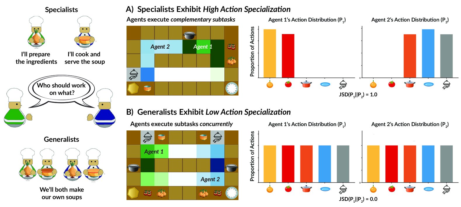
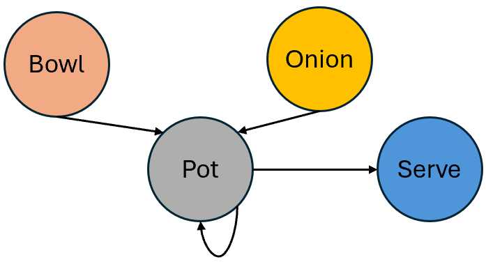
However, human teams demonstrate that specialization is not always optimal. Fine dining chefs coordinate to produce complex meals, but at the cost of high training overhead, rigidity, and failure risk if a key specialist is unavailable (Ben-Oren et al., 2023; Vélez et al., 2024). In contrast, generalist fry cooks perform the same subtasks in parallel, such as grilling and assembling, maximizing adaptability and throughput. Examples of specialist and generalist strategies are depicted in Figure 1. Furthermore, although AI agents also face coordination challenges (Shoham & Leyton-Brown, 2008; Wu et al., 2021), it remains unclear whether the constraints that make specialization advantageous for people also apply. With agents becoming increasingly capable we must revisit this assumption and ask: under what conditions, if any, is specialization truly optimal?
We propose that a task’s parallelizability—the potential for its independent subtasks to be executed simultaneously—limits the benefits of generalist teams. Drawing from the distributed computing literature (Almasi & Gottlieb, 1994; McCool et al., 2012; Vélez et al., 2023), we use Amdahl’s Law to determine when multi-agent systems should favor generalists or specialists. Amdahl’s Law predicts that there are diminishing returns to increasing the number of processors performing a task in parallel, based on the portion of the task that must be performed serially (Amdahl, 1967; Hill & Marty, 2008; Cassidy & Andreou, 2011). Applied to multi-agent systems, this places an upper bound on performance gains achievable from generalist agents working in parallel. When spatial and resource constraints limit parallel execution, agents should improve efficiency by specializing in complementary subtasks. Using a simple, interpretable model, we provide a novel framework for evaluating the trade-offs between specialist and generalist strategies.
To test this prediction, we develop a theoretical framework for comparing generalist and specialist efficiency and apply it to three multi-agent experiments in Overcooked-AI. Experiment 1 shows that key model variables influence specialization, with a moderate negative correlation between predicted task parallelizability and specialization, though larger state spaces complicate this relationship. Experiment 2 controls for these confounds, demonstrating our model’s high accuracy in predicting specialization. Experiment 3 finds that larger state spaces promote specialization by increasing coordination challenges. Our findings suggest that specialization is driven by task parallelizability and environment, enabling the design of layouts that encourage or inhibit policy diversity. More broadly, our framework highlights the value of using insights from distributed computing to improve the interpretability of multi-agent systems.
2 Theoretical Framework
We introduce a general framework for evaluating task parallelizability and predicting emergent specialization in multi-agent systems.
2.1 -Player Markov Game
Following Carroll et al. (2019) and Ruhdorfer et al. (2024), we formalize a cooperative decentralized Markov decision process (MDP), defined as . is a finite set of states, and is a set of agents. is the joint action space, where each agent selects an action to form a joint action . is the transition function which defines the probability distribution over next states given the current state and joint action. Finally, is the shared reward function. The objective of each agent is to maximize its expected discounted return , where is a discount factor and is the shared reward received by all agents at time . While agents share the same reward, each optimizes its own cumulative return independently.
2.2 Jensen-Shannon Divergence and Specialization
We define specialization as the differentiation of agents’ policies, capabilities, or roles in a multi-agent task. Let be the policy of agent that maps each state to a distribution over actions . In generalist teams, agents do not specialize in specific subtasks, and thus select from the entire set of actions . Formally, . In specialist teams, agents are restricted to specific subtasks and resources. In this case, , and their specialist policies satisfy . Examples of action distributions and specialist versus generalist strategies can be found in Figure 1.
Let the set of high-level actions be denoted as (Amato et al., 2019). Each agent follows a state-visitation distribution that describes how frequently they occupy different states under their policy (Schulman et al., 2015) given by:
| (1) |
The corresponding state-action visitation distribution is:
| (2) |
which represents the frequency with which an agent selects action in state under policy . For each agent , we define their effective action distribution using their visitation distribution:
| (3) |
This distribution captures both what actions an agent tends to take and how often they visit states where those actions are available. We approximate specialization using the Jensen-Shannon divergence (JSD) over agents’ action distributions (Endres & Schindelin, 2003; Fuglede & Topsoe, 2004). Given agents with action distributions , JSD is given by:
| (4) |
where is the mixture distribution, , and is the Kullback-Leibler (KL) divergence between each agent’s action distribution and . When , all agents have performed the same proportions of actions, indicating that all agents have performed all subtasks equally (no specialization). When , the action distributions are completely disjoint (i.e., each agent assigns probability exclusively to a unique set of actions with no overlap), meaning that the agents specialize in complementary subtasks. Intermediate values of JSD indicate partial specialization, in which the agents overlap in some subtasks but not others. We use Jensen-Shannon rather than Kullback-Leibler divergence because it is symmetric, i.e. . The degree of specialization in each team should be the same regardless of which agent specializes in which subtasks.
2.3 Graphical Representations of Spatial Layouts
To model task execution in structured environments, we represent spatial layouts as graphs. This allows for efficient computation of movement paths, bottlenecks, and spatial constraints on multi-agent coordination. We define a layout graph , where is the set of walkable positions and task-relevant objects and is the set of valid movements between adjacent positions. This spatial representation applies broadly to spatio-temporal multi-agent environments, including gridworlds. defines the static structure of the environment and constrains the MDP, where the state space includes agent positions and task-relevant object states. The transition function ensures that agents execute valid movements along edges in .
Definition 2.1.
A layout graph is an unweighted, directed graph where:
An edge exists if and only if and are adjacent, i.e., they share a horizontal or vertical edge in the grid. The type of edge between and depends on the type of nodes: (i) If and are both walkable nodes, there is a bidirectional edge such that and . (ii) If is a task-relevant object (e.g., workstation) there is a unidirectional edge , but , reflecting the fact that agents can interact with but not move through it.
2.4 Task Decomposition as a Directed Acyclic Graph
To analyze task parallelizability, we represent task execution as a directed acyclic graph (DAG), where nodes denote subtasks and edges represent the order in which subtasks must be completed (Solway et al., 2014).
Definition 2.2.
We define a task graph , where (subtask nodes) represent intermediate steps such as workstations or resources, and indicate ordering constraints between subtasks (e.g., an agent must retrieve an item before assembling it).
The number of subtasks depends on task complexity. Using the layout graph , we determine the spatial locations and paths between subtasks. The fraction of the total task spent on a given subtask is:
| (5) |
where is the path length required to complete subtask .
2.5 Spatial and Resource Bottlenecks
We introduce a framework to identify bottlenecks that constrain parallelizability in multi-agent tasks. This idea is inspired by sequential dependencies, resource contention, and communication overhead that prevent scalability in parallel processing (Almasi & Gottlieb, 1994; McCool et al., 2012; Zhuravlev et al., 2010). A classic example is memory bandwidth in GPUs, where increasing the number of threads does not lead to proportional speed-up due to limited shared access (Dublish et al., 2017). We extend this framework to multi-agent tasks by identifying two key types of bottlenecks: (1) spatial bottlenecks () limit movement of multiple agents due to obstacles, narrow passages, and congestion, and (2) resource bottlenecks () limit access to critical resources such as workstations or tools needed to complete subtasks (Mieczkowski et al., 2024). Together, these bottlenecks determine how effectively agents can execute tasks in parallel. They arise across numerous multi-agent domains, including warehouse operations (insufficient space, storage locations, and pallets (Živičnjak et al., 2022)), autonomous vehicles (lane reductions, traffic congestion (Zhang & Gao, 2020)), and smart factories (Wang et al., 2016).
We represent spatial and resource bottlenecks as two global sets over : , , where consists of edges in that constrain movement and consists of nodes in with task-relevant objects (e.g., workstations). Each subtask is constrained by a subset of bottlenecks relevant to the path () and resources () required to complete it.
To quantify spatial bottlenecks, we compute edge betweenness centrality, a graph-theoretic measure of congestion where high-centrality edges indicate critical bottlenecks in connectivity (Barrat et al., 2004).
Definition 2.3.
The betweenness centrality of an edge in graph is:
| (6) |
where is the number of shortest paths between nodes and , and is the number of those paths that pass through edge .
Since not all bottlenecks affect every subtask, we compute a per-subtask spatial bottleneck score by summing the centralities of all edges along the shortest path required for that subtask: , where path is the shortest path between subtask-relevant nodes and . A higher indicates stronger spatial constraints that may inhibit parallel agent movement.
To quantify resource bottlenecks, we simply sum the number of task-relevant nodes that are required for a subtask . For example, in a manufacturing system there may be only two welding stations; thus, only two agents may complete that subtask at the same time. Formally, for each subtask , we define a resource bottleneck score as: , where is the capacity of each task-relevant node (or the maximum agents that can use it at once).
2.6 Task Parallelizability Prediction
We now adapt Amdahl’s Law, a measure of the expected speed-up when dividing a task across multiple processors given the proportion that must be executed serially, to multi-agent tasks (Amdahl, 1967; Hill & Marty, 2008; Cassidy & Andreou, 2011). For the original form of Amdahl’s Law, see Appendix A.1. Mieczkowski et al. (2024) extended this idea to predict idleness during human collaborations given the current group size, workload, and resource constraints. We hypothesize that a similar formulation can be used to predict specialization in multi-agent tasks.
Let represent the fraction of the total task time required for the of subtasks such that . For each subtask , the overall bottleneck capacity is defined as the minimum bottleneck that prevents agents executing it concurrently, or . The subtask speed-up factor quantifies the efficiency gain from adding an th agent to a subtask, given that agents are already working on it and bottlenecks restrict parallel execution. Formally:
| (7) |
Thus, if we assume that there is no cost to switching between subtasks, the overall expected speed-up achievable when an additional agent performs the entire task in parallel, which we call task parallelizability, is expressed as:
| (8) |
2.7 Task Parallelizability and Specialization
Our task parallelizability prediction estimates the efficiency gain if an additional agent independently completed all subtasks in parallel. We propose that this measure sets a fundamental upper bound on the benefits of specialization in multi-agent systems. If is low due to resource or spatial bottlenecks, then the task would not be significantly sped up by multiple agents executing it in parallel. In this case, there would be little value to a team of generalist agents, so if we want to increase task efficiency it is better for agents to specialize and perform complementary subtasks. However, specialization itself can introduce new bottlenecks, particularly when agents must coordinate frequently or wait for specific subtasks to be completed before proceeding. In environments with high parallelizability , generalist agents who work independently may avoid these delays, leading to faster performance.
3 Application to Overcooked-AI
To investigate how task parallelizability influences specialization, we apply our theoretical model for predicting generalist efficiency to a specific multi-agent environment (Carroll et al., 2019). Overcooked-AI is a fully cooperative two-agent platform in which pairs of agents must deliver soups as quickly as possible while navigating obstacles, avoiding collisions, and coordinating subtasks (Wu et al., 2021). Each recipe requires a different number of subtasks () to prepare a soup, while resource bottlenecks such as the number of pots () and spatial bottlenecks such as narrow passages () constrain task parallelizability.
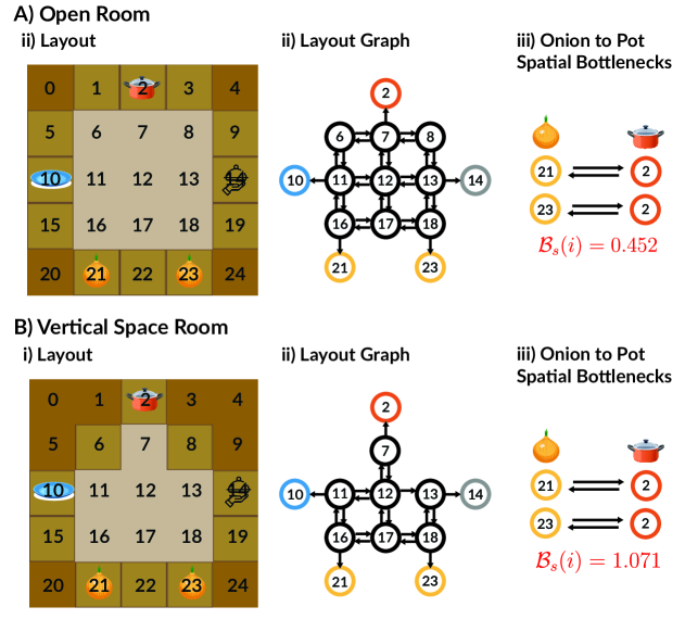
Layout Graphs. We represent each layout graph according to Definition 2.1. An example is depicted in Figure 2.
Task Decomposition. We decompose the overall task of “cooking a soup” using a directed acyclic graph (DAG) according to Definition 2.2, where is the set of resources, or workstations (e.g., onion piles, pots, bowls), and is a directed edge representing a required subtask (such as moving an onion to the pot). An example can be found in Figure 5. The number of subtasks depends on the recipe. To make a one-onion soup, there are subtasks total: Onion Pot, Cook in Pot, Bowl Pot, and Pot Serve. To make a two-onion or one-onion one-tomato soup, there are subtasks. To make a three-onion or two-onion one-tomato soup, there are subtasks. Using the layout graph , we determine the locations and paths between workstations. The fraction spent on subtask is its path length relative to the total path length of all subtasks following Equation 5.
Bottlenecks. We manipulate and measure bottlenecks in Overcoooked in two ways. We vary resource bottlenecks by changing the number of workstations ( pots, onions, tomatoes, bowls, and serving stations) available to agents. We vary spatial bottlenecks by modifying the layout size and arrangement of obstacles (represented as counters that agents cannot cross). We quantify these spatial bottlenecks for each subtask using edge betweenness centrality as described in Definition 2.3.
Specialization. To measure specialization, we convert agents’ behaviors (move, interact, wait) from a policy roll-out of the best-performing seed to high-level actions: (i) picking up onions, (ii) placing onions in pot, (iii) picking up tomatoes, (iv) placing tomatoes in pot, (v) picking up bowls, (vi) moving soup from pot to bowl, and (vii) serving soup. Each agent has an action distribution , where represents the probability of agent taking action during a policy roll-out after training. For each agent , we compute their high-level action distribution by normalizing the frequency of each action over the total actions they performed during the roll-out. We measure specialization as the Jensen-Shannon divergence between agents, .
Task Parallelizability Prediction. Our model for predicting task parallelizability measures the relative efficiency gained from two generalist agents making soups in parallel versus specializing in subtasks (e.g., fetching ingredients versus serving soup). Consider the task of making one-onion soup. This requires subtasks: Onion Pot, Cook in Pot, Bowl Pot, and Pot Serve. Each subtask is associated with (i) a number of workstations , (ii) a path length , and (iii) a measure of spatial bottlenecks between those workstations, where indicates constrained areas. If there are multiple paths, we consider . Subtask durations are weighted by path length (Equation 5), with Cook assumed to take 10 time-steps. The overall speed-up expected from two generalist agents making soups in parallel is thus given by in Equation 8. We hypothesize an inverse relationship between and . This would suggest agents specialize more when task and environmental constraints inhibit them from executing the same subtasks simultaneously.
4 Experiment 1: Exploring Specialization in Large-Scale Overcooked Simulations
In Experiment 1, we conduct a large-scale analysis across a variety of environments to test whether parallelizability impacts the emergence of specialization.
4.1 Experiment Design
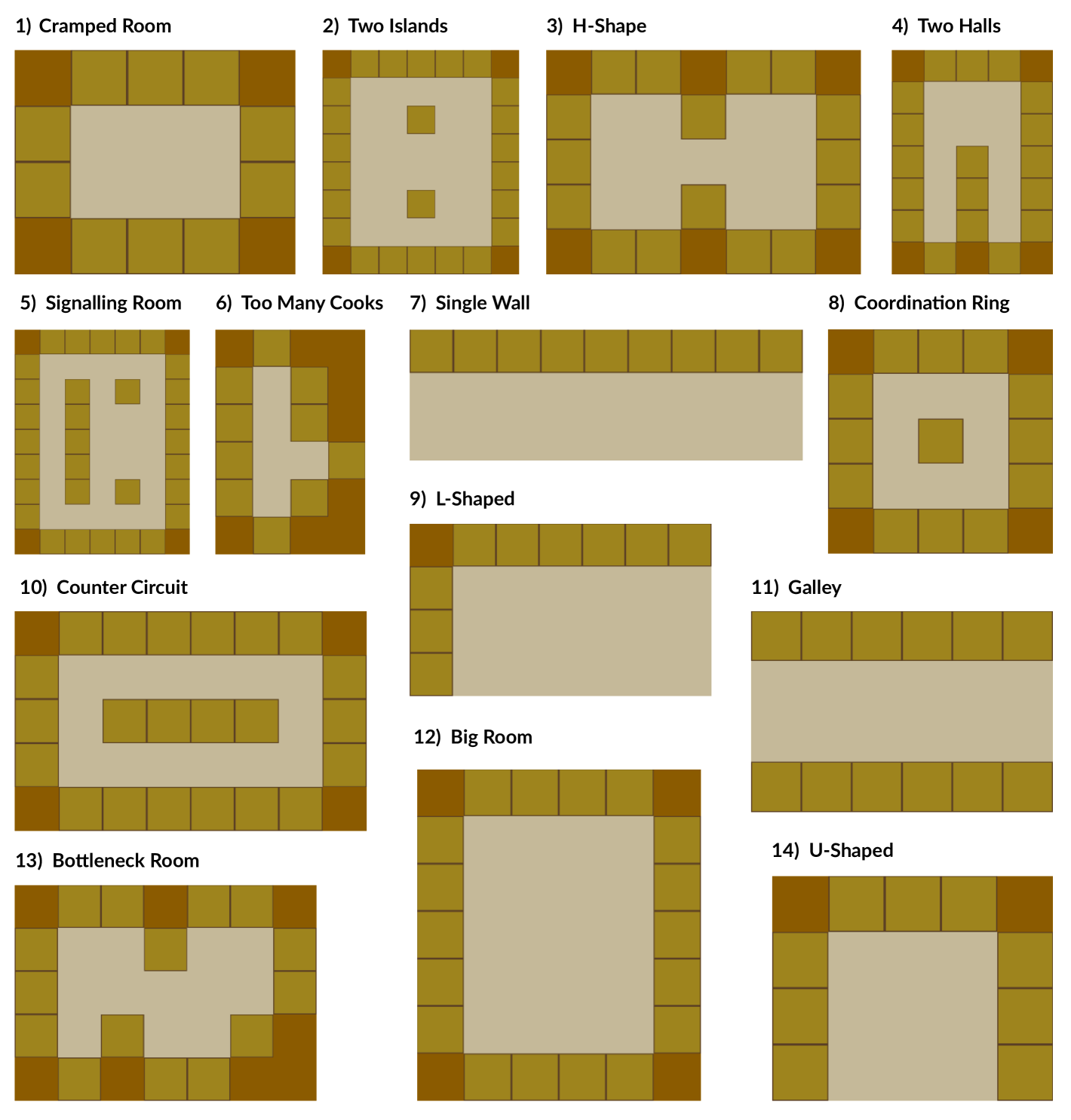
We generated a test suite of 3,200 unique Overcooked environments for exploratory analysis. We utilized 14 spatial configurations representing 2D gridworld kitchens, each with a unique arrangement of counters and floor areas, including the original layouts from Overcooked-AI and a new set of layouts inspired by real-world kitchens (Pejic et al., 2019). A complete set of layouts is provided in Figure 6. To create diverse parallelizability constraints, we systematically varied the number of workstations (onions, tomatoes, pots, bowls, and serving stations). A total of 16 combinations included one or two onion piles, bowls, pots, serving stations, and zero or one tomatoes. Workstation positions were randomized three times per layout. Agents were trained to make five recipes: (i) 1-onion (ii) 2-onion (iii) 3-onion (iv) 1-onion and 1-tomato and (v) 2-onion and 1-tomato soup. These variations produced a total of 3,200 unique environments. For each of these environments, we trained two independent agents to play Overcooked collaboratively via self-play using PureJaxRL and PPO with five random seeds (Schulman et al., 2017; Lu et al., 2022). Full details regarding training procedures can be found in Appendix A.3. We then selected the highest-performing seed based on the joint reward that agents achieved during the roll-out. If multiple seeds reached the same maximum reward, we averaged their JSD. Trials were excluded if agents failed to take high-level actions or achieved a roll-out reward of 0.
4.2 Results
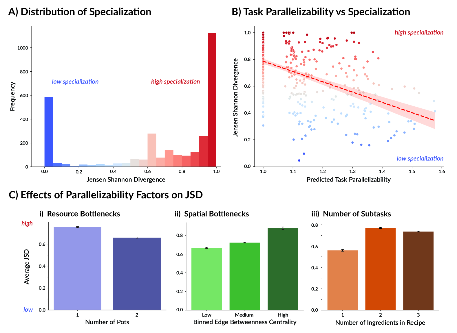
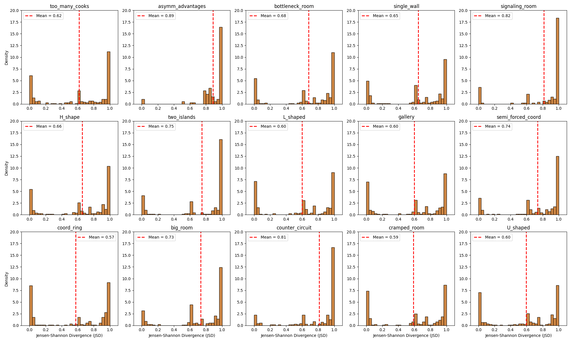
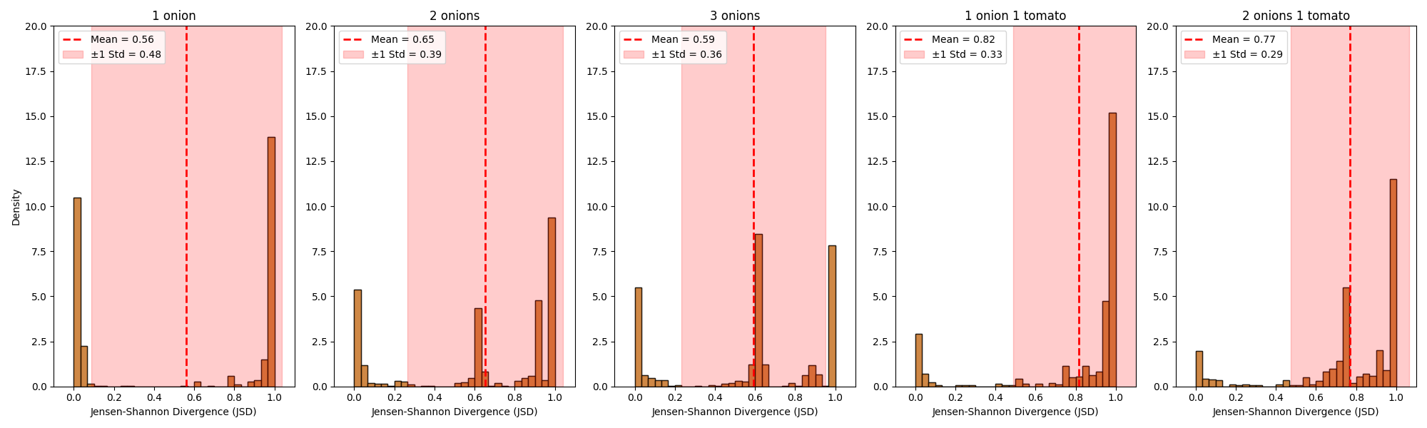
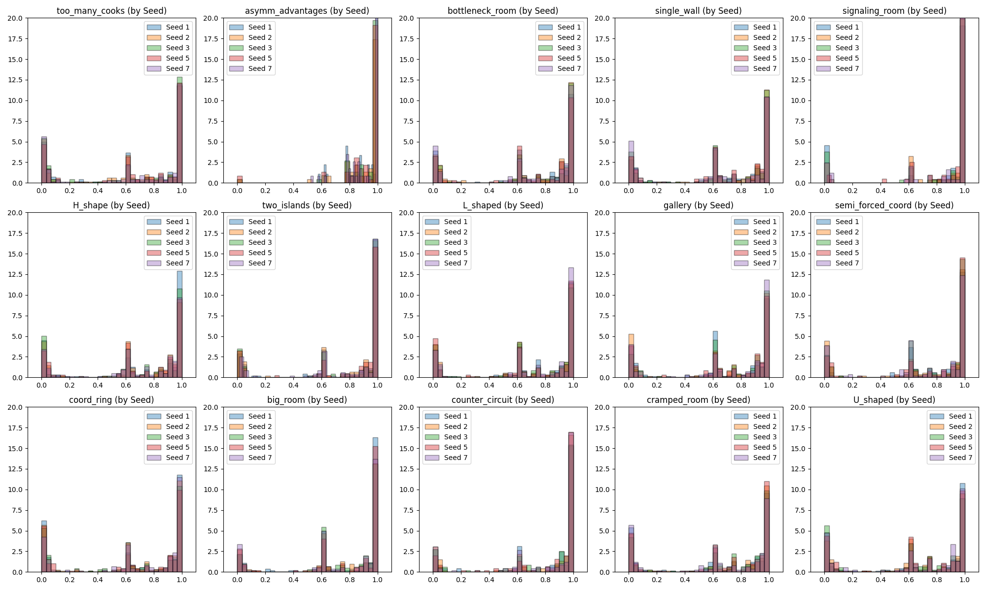
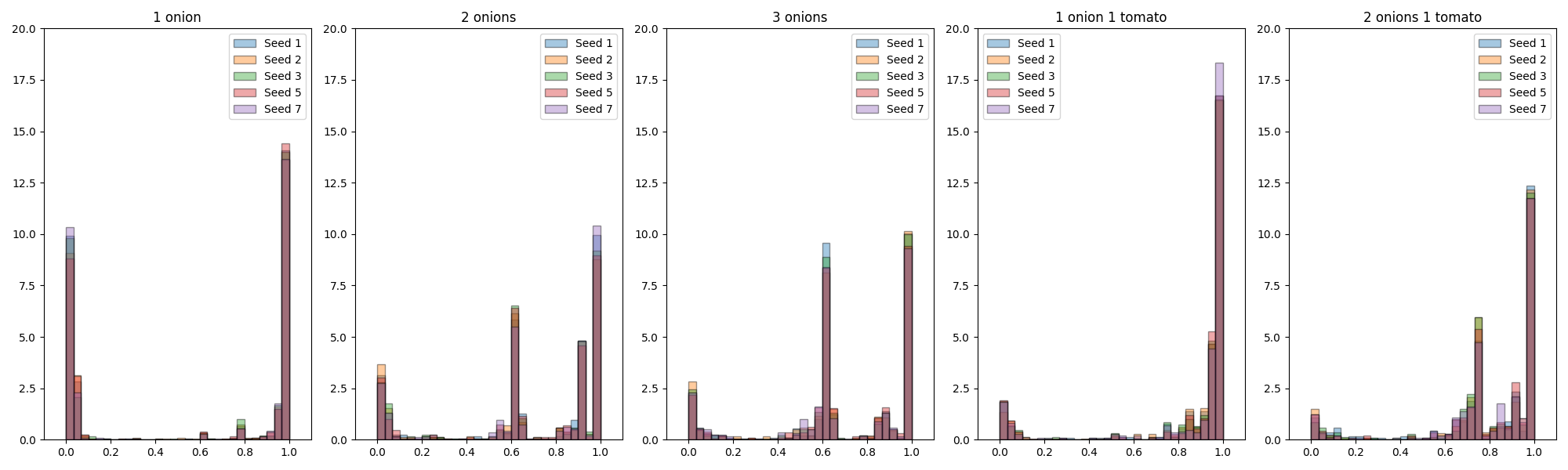
Distribution of JSD. Results from Experiment 1 are depicted in Figure 3. Our simulations revealed two distinct behavioral modes. Specialists () dominated of runs, with fully specialized (). Generalists () appeared in of runs, including fully generalist (). The remaining exhibited mixed specialist-generalist behaviors ().
Effects of Parallelizability on Specialization. For each of the variables presented in our predictive model, there was a significant effect in the expected direction on observed JSD. Full statistical details can be found in Appendix A.4. We found a significant effect of the number of pots, but not the total number of workstations; spatial bottlenecks; and recipe complexity (the number of ingredients required to make a soup) on emergent specialization.
Model Evaluation. We analyzed the relationship between predicted task parallelizability and observed specialization (JSD) across 14 Overcooked layouts. Full statistical details are in Appendix A.5, with Tables 1 and 2 summarizing correlations, JSD, and rewards. The average correlation () revealed a moderate negative relationship between generalist efficiency and JSD, supporting our hypothesis that greater task parallelizability predicts lower specialization. A logistic regression classifying low vs. high specialization () achieved accuracy, with precision () for high specialization and precision () for low specialization.
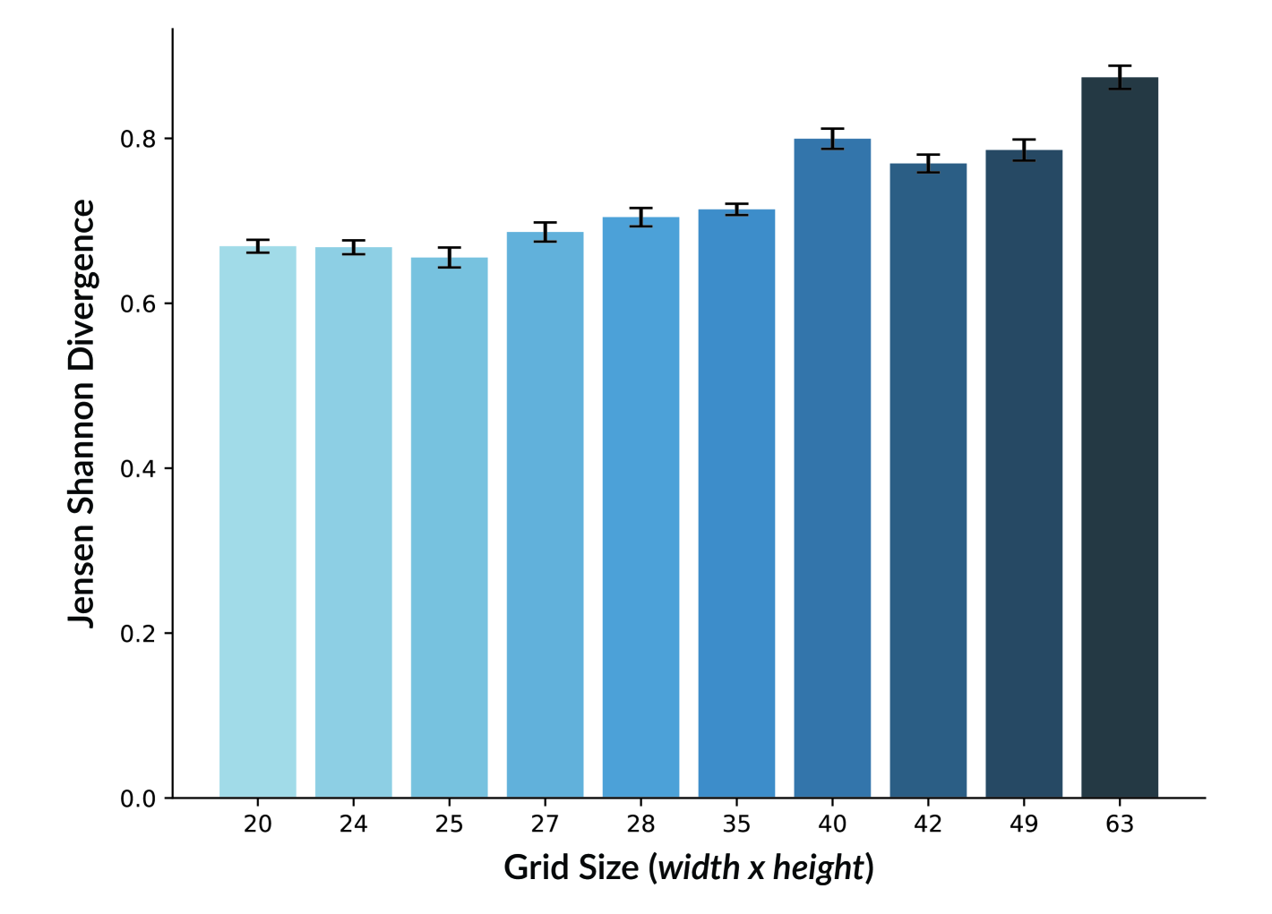
Effects of State Space on Specialization We also observed a moderate correlation between grid size and average JSD (), even when controlling for resource and spatial bottlenecks (Figure 7). This suggests that state space size and workstation distances may act as confounding variables, influencing specialization independently of task-specific constraints. Larger state spaces increase exploration demands. In response, agents may adopt specialization as a locally optimal strategy to reduce policy complexity by focusing on specific paths and workstation interactions.
5 Experiment 2: Validating Predictive Model
In Experiment 1, we confirmed that the variables which should affect generalist strategies from speeding up task completion have a significant impact on specialization. In Experiment 2, we validate our results using a smaller, controlled experiment. We also show that we can use our findings to design environments which will induce or inhibit the emergence of specialized roles.
5.1 Experiment Design
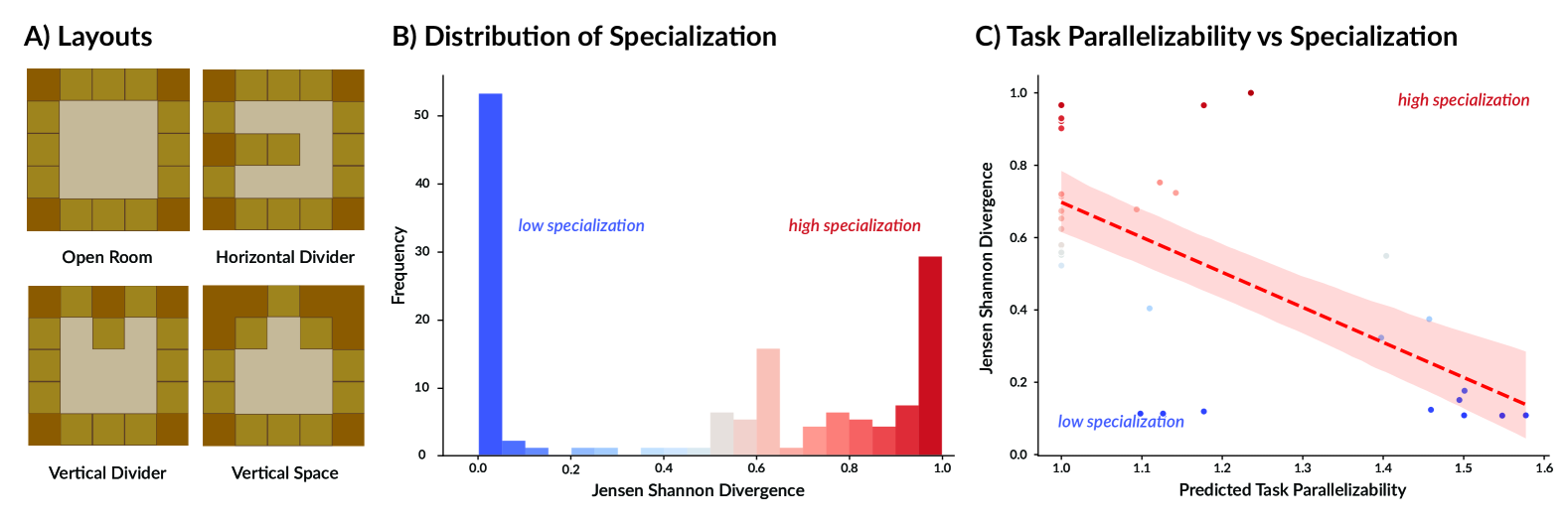
We utilized the same methods, game dynamics, and training schemes as in Experiment 1 (described in Section 4.1). To control state space size while varying spatial bottlenecks, we constructed six grid layouts: (1) open space with surrounding counters, (2) single vertical divider, (3) double vertical divider and (4) horizontal divider. These spatial layouts are illustrated in Figure 4. We varied the number of pots (1 or 2) rather than workstations, since pots had the largest effect on specialization in Experiment 1, while controlling for relative distances between workstations across trials. Each layout featured four workstation arrangements, totaling 48 configurations. For each, agents were trained to make one-, two-, or three-onion soup with 10 random seeds for a total of 1400 runs. As in Experiment 1, we again selected the highest-performing seed in terms of the joint reward that agents achieved during the policy roll-out after averaging over the randomized locations of workstations. Four trials were excluded from Experiment 2.
5.2 Results
Results from Experiment 2 are depicted in Figure 4. By fixing the size of the grid, the distinction between generalist and specialist strategies became more pronounced, with a clear bimodal distribution emerging. There were 81 specialist teams with () and 59 generalist teams (). Notably, the proportion of generalists increased substantially compared to Experiment 1 once we removed the confound of altering layout size, providing further evidence that specialization is partially driven by the size of the state space. Additionally, our predictive model achieved even greater accuracy for predicting specialization. The Pearson correlation between predicted task parallelizability and JSD was (), confirming the hypothesized inverse relationship between generalist efficiency and specialization. Statistical details can be found in Appendix A.6. To validate the model’s predictive power, we fit a class-balanced logistic regression to classify high () or low specialization (). The model achieved a test set accuracy of , demonstrating strong performance with precision () for high specialization and precision () for low.
These results suggest that spatial bottlenecks and resource availability are key factors driving the emergence of specialization. Our findings indicate that our predictive model can be used to systematically design environments that will either promote or inhibit specialization. Rather than tailoring training algorithms to induce policy diversity, it is possible to do so based on environmental design alone. If agents are given ample space and workstations to learn the task, they will develop emergent generalist behaviors. Alternatively, if the environment is constrained spatially or in terms of resources, agents will develop specialist roles.
6 Experiment 3: Investigating State Space Size and Specialization
In Experiment 3, we investigate the relationship between state space size and specialization in greater detail. Our findings show that as the state space expands, even if the size of the grid that the agents can explore is held constant, agents consistently converge on more specialized strategies, indicating that specialization is a less computationally costly alternative when learning is made more difficult. These findings highlight a challenge in MARL: as state spaces grow, agents struggle to converge on optimal generalist policies. Full details, including the experimental design, results and statistical analysis are provided in Appendix A.7 and A.8.
7 Related Work
The study of specialization in multi-agent systems spans multiple disciplines. Division of labor leading to functional specialization has been widely studied in biological and social domains, including cells (Bell & Mooers, 1997; Rueffler et al., 2012), insect colonies (Ratnieks & Anderson, 1999; Fjerdingstad & Crozier, 2006), and human societies (Kitcher, 1990; Kreider et al., 2022; Goldstone et al., 2024; Vélez et al., 2024). Inspired by these insights, research in MARL and robotics has sought to design algorithms that actively encourage specialization by promoting policy diversity (Murciano et al., 1997; Padgham & Winikoff, 2002; Zhu & Zhou, 2008; Charakorn et al., 2020; Wang et al., 2020a, b; Li et al., 2021; Bettini et al., 2023, 2024) or by organizing agents into hierarchies (Zhang et al., 2010; Ahilan & Dayan, 2019). Similarly, new work on language-agent collaboration often assumes that specialization is necessary, prompting agents to adopt distinct roles before collaborating (Wang et al., 2023; Suzgun & Kalai, 2024; Swanson et al., 2024; Liu et al., 2024; Juang et al., 2024). However, much of this work assumes that specialization is always beneficial, without systematically identifying when and why generalist strategies may outperform specialists. A useful contrast comes from distributed systems, which are explicitly engineered rather than emergent. In these systems, heterogeneity and parallelism are carefully designed to optimize performance (Moncrieff et al., 1996; Almasi & Gottlieb, 1994; Pancake, 1996) and minimize contention (Park & Reveliotis, 2001). This structured approach provides a useful reference point for understanding when emergent specialization is not just incidental, but optimal.
While biological and social systems provide compelling examples, it remains an open question when specialization emerges as the optimal architecture. Prior work suggests that under conditions of high environmental variability or individual failure, flexible generalist strategies may outperform rigidly specialized roles (Staps & Tarnita, 2022; Ben-Oren et al., 2023). In our work, we propose a novel theoretical framework for predicting the utility of specialization based on task efficiency, considering environmental bottlenecks, resource constraints, and task complexity. Prior work in RL has shown that spatial bottlenecks such as doorways can shape subgoals (Menache et al., 2002), while research in human-robot collaboration and MARL has demonstrated that environmental design influences emergent behavior (Fontaine et al., 2021; McKee et al., 2022). Building on these insights, we formalize a predictive model for when generalist versus specialist strategies should emerge.
8 Discussion
Specialization, or the differentiation of agents’ policies and roles, is often assumed to improve collaborative performance. However, principles from distributed systems offer an alternative hypothesis. Specifically, generalist agents may outperform specialist ones when concurrent execution of the entire task would improve speed and efficiency. In this work, we outlined a theoretical framework for predicting generalist versus specialist efficiency in cooperative multi-agent tasks inspired by a variant of Amdahl’s Law. We then validated this model across three Overcooked experiments, finding highly significant effects of parallelizability factors on emergent specialization and high predictive accuracy. Together, these findings suggest that specialization is constrained by the environment and parallelizability of a task, making it possible to design layouts which either encourage or inhibit role emergence regardless of whether the training algorithm explicitly incentivizes diversity. More broadly, this framework motivates the use of distributed systems in analyzing trade-offs that arise when dividing labor.
This work has several limitations. First, our model does not account for switching behavior (generalists who switch roles rather than cooking independently) or cases where specialist and generalist policies are equally optimal. This limitation arises from an implicit assumption from Amdahl’s Law that subtasks are executed sequentially without overlap. Second, our model provides a theoretical upper bound on the benefits of generalists, but does not account for potential coordination overhead when increasing the number of agents, which could make the empirical relationship non-monotonic. Third, our model assumes agents are equally capable, yet specialization can also arise when agents have heterogeneous skills that make them more efficient at certain tasks (Moncrieff et al., 1996; Ginting et al., 2022). Despite these limitations, our predictive model is highly extensible. It generalizes from 2 to agents, providing explicit predictions for larger teams. Finally, our work suggests that specialization is a locally optimal solution that agents use when exploration is costly, i.e. in larger state spaces. Clarifying this trade-off can provide insight into how specialization may improve sample efficiency, as well as how to decrease coordination overhead between agents.
Acknowledgments
This work was supported in part by the Department of Defense (DoD) through the National Defense Science and Engineering Graduate (NDSEG) Fellowship Program, the Office of Naval Research (ONR) MURI grant (N00014-22-1-2813), the EPSRC CDT in RAS (EP/L016834/1), and a grant from the Templeton World Charity Foundation.
References
- Ahilan & Dayan (2019) Ahilan, S. and Dayan, P. Feudal multi-agent hierarchies for cooperative reinforcement learning. arXiv preprint arXiv:1901.08492, 2019.
- Almasi & Gottlieb (1994) Almasi, G. S. and Gottlieb, A. Highly parallel computing. Benjamin-Cummings Publishing Co., 1994.
- Amato et al. (2019) Amato, C., Konidaris, G., Kaelbling, L. P., and How, J. P. Modeling and planning with macro-actions in decentralized pomdps. Journal of Artificial Intelligence Research, 64:817–859, 2019.
- Amdahl (1967) Amdahl, G. M. Validity of the single processor approach to achieving large scale computing capabilities. In Proceedings of the April 18-20, 1967, Spring Joint Computer Conference, pp. 483–485, 1967.
- Barrat et al. (2004) Barrat, A., Barthelemy, M., Pastor-Satorras, R., and Vespignani, A. The architecture of complex weighted networks. Proceedings of the National Academy of Sciences, 101(11):3747–3752, 2004.
- Bell & Mooers (1997) Bell, G. and Mooers, A. O. Size and complexity among multicellular organisms. Biological Journal of the Linnean Society, 60(3):345–363, 1997.
- Ben-Oren et al. (2023) Ben-Oren, Y., Kolodny, O., and Creanza, N. Cultural specialization as a double-edged sword: division into specialized guilds might promote cultural complexity at the cost of higher susceptibility to cultural loss. Philosophical Transactions of the Royal Society B, 378(1872):20210418, 2023.
- Bettini et al. (2023) Bettini, M., Shankar, A., and Prorok, A. Heterogeneous multi-robot reinforcement learning. arXiv preprint arXiv:2301.07137, 2023.
- Bettini et al. (2024) Bettini, M., Kortvelesy, R., and Prorok, A. Controlling behavioral diversity in multi-agent reinforcement learning. arXiv preprint arXiv:2405.15054, 2024.
- Canese et al. (2021) Canese, L., Cardarilli, G. C., Di Nunzio, L., Fazzolari, R., Giardino, D., Re, M., and Spanò, S. Multi-agent reinforcement learning: A review of challenges and applications. Applied Sciences, 11(11):4948, 2021.
- Carroll et al. (2019) Carroll, M., Shah, R., Ho, M. K., Griffiths, T., Seshia, S., Abbeel, P., and Dragan, A. On the utility of learning about humans for human-AI coordination. Advances in Neural Information Processing Systems, 32, 2019.
- Cassidy & Andreou (2011) Cassidy, A. S. and Andreou, A. G. Beyond Amdahl’s law: An objective function that links multiprocessor performance gains to delay and energy. IEEE Transactions on Computers, 61(8):1110–1126, 2011.
- Charakorn et al. (2020) Charakorn, R., Manoonpong, P., and Dilokthanakul, N. Investigating partner diversification methods in cooperative multi-agent deep reinforcement learning. In International Conference on Neural Information Processing, pp. 395–402, 2020.
- Dublish et al. (2017) Dublish, S., Nagarajan, V., and Topham, N. Evaluating and mitigating bandwidth bottlenecks across the memory hierarchy in gpus. In IEEE International Symposium on Performance Analysis of Systems and Software (ISPASS), pp. 239–248, 2017.
- Endres & Schindelin (2003) Endres, D. M. and Schindelin, J. E. A new metric for probability distributions. IEEE Transactions on Information Theory, 49(7):1858–1860, 2003.
- Fjerdingstad & Crozier (2006) Fjerdingstad, E. J. and Crozier, R. H. The evolution of worker caste diversity in social insects. The American Naturalist, 167(3):390–400, 2006.
- Fontaine et al. (2021) Fontaine, M. C., Hsu, Y.-C., Zhang, Y., Tjanaka, B., and Nikolaidis, S. On the importance of environments in human-robot coordination. arXiv preprint arXiv:2106.10853, 2021.
- Fuglede & Topsoe (2004) Fuglede, B. and Topsoe, F. Jensen-Shannon divergence and Hilbert space embedding. In International Symposium on Information Theory, pp. 31, 2004.
- Ginting et al. (2022) Ginting, M. F., Otsu, K., Kochenderfer, M. J., and Agha-Mohammadi, A.-A. Capability-aware task allocation and team formation analysis for cooperative exploration of complex environments. In International Conference on Intelligent Robots and Systems, pp. 7145–7152, 2022.
- Goldstone et al. (2024) Goldstone, R. L., Andrade-Lotero, E. J., Hawkins, R. D., and Roberts, M. E. The emergence of specialized roles within groups. Topics in Cognitive Science, 16(2):257–281, 2024.
- Griffiths (2020) Griffiths, T. L. Understanding human intelligence through human limitations. Trends in Cognitive Sciences, 24(11):873–883, 2020.
- Haarnoja et al. (2018) Haarnoja, T., Zhou, A., Abbeel, P., and Levine, S. Soft actor-critic: Off-policy maximum entropy deep reinforcement learning with a stochastic actor. In International Conference on Machine Learning, pp. 1861–1870, 2018.
- Hill & Marty (2008) Hill, M. D. and Marty, M. R. Amdahl’s law in the multicore era. Computer, 41(7):33–38, 2008.
- Juang et al. (2024) Juang, S., Cao, H., Zhou, A., Liu, R., Zhang, N. L., and Liu, E. Breaking the mold: The challenge of large scale MARL specialization. arXiv preprint arXiv:2410.02128, 2024.
- Kitcher (1990) Kitcher, P. The division of cognitive labor. The journal of philosophy, 87(1):5–22, 1990.
- Kreider et al. (2022) Kreider, J. J., Janzen, T., Bernadou, A., Elsner, D., Kramer, B. H., and Weissing, F. J. Resource sharing is sufficient for the emergence of division of labour. Nature Communications, 13(1):7232, 2022.
- Li et al. (2021) Li, C., Wang, T., Wu, C., Zhao, Q., Yang, J., and Zhang, C. Celebrating diversity in shared multi-agent reinforcement learning. Advances in Neural Information Processing Systems, 34:3991–4002, 2021.
- Liu et al. (2024) Liu, Z., Zhang, Y., Li, P., Liu, Y., and Yang, D. A dynamic LLM-powered agent network for task-oriented agent collaboration. In First Conference on Language Modeling, 2024.
- Lu et al. (2022) Lu, C., Kuba, J. G., Letcher, A., Metz, L., de Witt, C. S., and Foerster, J. Discovered policy optimisation. Advances in Neural Information Processing Systems, 2022.
- McCool et al. (2012) McCool, M., Reinders, J., and Robison, A. Structured parallel programming: Patterns for efficient computation. Elsevier, 2012.
- McKee et al. (2022) McKee, K. R., Leibo, J. Z., Beattie, C., and Everett, R. Quantifying the effects of environment and population diversity in multi-agent reinforcement learning. Autonomous Agents and Multi-Agent Systems, 36(1):21, 2022.
- Menache et al. (2002) Menache, I., Mannor, S., and Shimkin, N. Q-cut—dynamic discovery of sub-goals in reinforcement learning. In 13th European Conference on Machine Learning, pp. 295–306, 2002.
- Mieczkowski et al. (2024) Mieczkowski, E. A., Turner, C. R., Vélez, N., and Griffiths, T. L. People evaluate idle collaborators based on their impact on task efficiency. PsyArXiv, 2024.
- Moncrieff et al. (1996) Moncrieff, D., Overill, R. E., and Wilson, S. Heterogeneous computing machines and Amdahl’s Law. Parallel Computing, 22(3):407–413, 1996.
- Murciano et al. (1997) Murciano, A., del R. Millán, J., and Zamora, J. Specialization in multi-agent systems through learning. Biological Cybernetics, 76(5):375–382, 1997.
- Padgham & Winikoff (2002) Padgham, L. and Winikoff, M. Prometheus: A methodology for developing intelligent agents. In Proceedings of the First International Joint Conference on Autonomous Agents and Multiagent Systems: Part 1, pp. 37–38, 2002.
- Pancake (1996) Pancake, C. Is parallelism for you? IEEE Computational Science and Engineering, 3(2):18–37, 1996.
- Park & Reveliotis (2001) Park, J. and Reveliotis, S. A. Deadlock avoidance in sequential resource allocation systems with multiple resource acquisitions and flexible routings. IEEE Transactions on Automatic Control, 46(10):1572–1583, 2001.
- Park et al. (2023) Park, J. S., O’Brien, J. C., Cai, C. J., Morris, M. R., Liang, P., and Bernstein, M. S. Generative agents: Interactive simulacra of human behavior. arxiv. arXiv preprint ArXiv:2304.03442, 2023.
- Pejic et al. (2019) Pejic, P., Jovanovic, D., Marinkovic, J., Stojakovic, V., and Krasic, S. Parametric 3D modeling of I-shape kitchen. Journal of Industrial Design and Engineering Graphics, 14(1):155–158, 2019.
- Perolat et al. (2017) Perolat, J., Leibo, J. Z., Zambaldi, V., Beattie, C., Tuyls, K., and Graepel, T. A multi-agent reinforcement learning model of common-pool resource appropriation. Advances in Neural Information Processing Systems, 30, 2017.
- Ratnieks & Anderson (1999) Ratnieks, F. L. and Anderson, C. Task partitioning in insect societies. Insectes Sociaux, 46:95–108, 1999.
- Rueffler et al. (2012) Rueffler, C., Hermisson, J., and Wagner, G. P. Evolution of functional specialization and division of labor. Proceedings of the National Academy of Sciences, 109(6):E326–E335, 2012.
- Ruhdorfer et al. (2024) Ruhdorfer, C., Bortoletto, M., Penzkofer, A., and Bulling, A. The Overcooked Generalisation Challenge. arXiv preprint arXiv:2406.17949, 2024.
- Schulman et al. (2015) Schulman, J., Levine, S., Abbeel, P., Jordan, M., and Moritz, P. Trust region policy optimization. In International conference on machine learning, pp. 1889–1897. PMLR, 2015.
- Schulman et al. (2017) Schulman, J., Wolski, F., Dhariwal, P., Radford, A., and Klimov, O. Proximal policy optimization algorithms. arXiv, 2017.
- Shoham & Leyton-Brown (2008) Shoham, Y. and Leyton-Brown, K. Multiagent systems: Algorithmic, game-theoretic, and logical foundations. Cambridge University Press, 2008.
- Solway et al. (2014) Solway, A., Diuk, C., Córdova, N., Yee, D., Barto, A. G., Niv, Y., and Botvinick, M. M. Optimal behavioral hierarchy. PLoS computational biology, 10(8):e1003779, 2014.
- Staps & Tarnita (2022) Staps, M. and Tarnita, C. E. When being flexible matters: Ecological underpinnings for the evolution of collective flexibility and task allocation. Proceedings of the National Academy of Sciences, 119(18):e2116066119, 2022.
- Suzgun & Kalai (2024) Suzgun, M. and Kalai, A. T. Meta-prompting: Enhancing language models with task-agnostic scaffolding. arXiv preprint arXiv:2401.12954, 2024.
- Swanson et al. (2024) Swanson, K., Wu, W., Bulaong, N. L., Pak, J. E., and Zou, J. The virtual lab: AI agents design new Sars-Cov-2 nanobodies with experimental validation. bioRxiv, pp. 2024–11, 2024.
- Vélez et al. (2023) Vélez, N., Christian, B., Hardy, M., Thompson, B. D., and Griffiths, T. L. How do humans overcome individual computational limitations by working together? Cognitive Science, 47(1):e13232, 2023.
- Vélez et al. (2024) Vélez, N., Wu, C. M., Gershman, S. J., and Schulz, E. The rise and fall of technological development in virtual communities. PsyArXiv, 2024.
- Wang et al. (2016) Wang, S., Wan, J., Zhang, D., Li, D., and Zhang, C. Towards smart factory for industry 4.0: A self-organized multi-agent system with big data based feedback and coordination. Computer Networks, 101:158–168, 2016.
- Wang et al. (2020a) Wang, T., Dong, H., Lesser, V., and Zhang, C. Roma: Multi-agent reinforcement learning with emergent roles. arXiv preprint arXiv:2003.08039, 2020a.
- Wang et al. (2020b) Wang, T., Gupta, T., Mahajan, A., Peng, B., Whiteson, S., and Zhang, C. Rode: Learning roles to decompose multi-agent tasks. arXiv preprint arXiv:2010.01523, 2020b.
- Wang et al. (2023) Wang, Z., Mao, S., Wu, W., Ge, T., Wei, F., and Ji, H. Unleashing the emergent cognitive synergy in large language models: A task-solving agent through multi-persona self-collaboration. arXiv preprint arXiv:2307.05300, 2023.
- Wu et al. (2021) Wu, S. A., Wang, R. E., Evans, J. A., Tenenbaum, J. B., Parkes, D. C., and Kleiman-Weiner, M. Too many cooks: Bayesian inference for coordinating multi-agent collaboration. Topics in Cognitive Science, 13(2):414–432, 2021.
- Zhang et al. (2010) Zhang, C., Lesser, V. R., and Abdallah, S. Self-organization for coordinating decentralized reinforcement learning. In Proceedings of the International Joint Conference on Autonomous Agents and Multiagent Systems, volume 10, pp. 739–746, 2010.
- Zhang & Gao (2020) Zhang, T. and Gao, K. Will autonomous vehicles improve traffic efficiency and safety in urban road bottlenecks? In International Conference on Intelligent Transportation Engineering (ICITE), pp. 366–370, 2020.
- Zhang (2018) Zhang, Z. Improved Adam optimizer for deep neural networks. In International Symposium on Quality of Service, pp. 1–2, 2018.
- Zhu & Zhou (2008) Zhu, H. and Zhou, M. Role-based multi-agent systems. In Personalized Information Retrieval and Access: Concepts, Methods and Practices, pp. 254–285. IGI Global, 2008.
- Zhuravlev et al. (2010) Zhuravlev, S., Blagodurov, S., and Fedorova, A. Addressing shared resource contention in multicore processors via scheduling. ACM Sigplan Notices, 45(3):129–142, 2010.
- Živičnjak et al. (2022) Živičnjak, M., Rogić, K., and Bajor, I. Case-study analysis of warehouse process optimization. Transportation Research Procedia, 64:215–223, 2022.
Appendix A Appendix
A.1 Original Form of Amdahl’s Law
Let represent the proportion of a task that can be parallelized and accelerated by a factor of , while denotes the portion that must be executed serially. The theoretical speedup achievable when distributing a task across multiple processors is given by:
| (9) |
A.2 Task Decomposition Graph
A.3 Training Procedures
For each trial in our MARL experiments, we trained two independent agents to play Overcooked collaboratively through self-play. Our implementation builds upon the PureJaxRL framework for Proximal Policy Optimization (Schulman et al., 2017; Lu et al., 2022). Each agent was implemented using an soft Actor-Critic network (Haarnoja et al., 2018), in which both the actor and critic networks were composed of two fully-connected layers with 64 hidden units each. We trained each agent using Proximal Policy Optimization with an Adam optimizer and a learning rate of for timesteps (Zhang, 2018). At each timestep, the agents observed the state of the current environment as a -dimensional grid. The first two dimensions corresponded to the spatial coordinates of the grid, while the 27-dimensional vector encoded the state of each grid cell, indicating whether it contained an agent, onion, tomato, bowl, or workstation. The policy produced a categorical distribution over discrete actions.
To accelerate learning in the sparse-reward environments, we applied reward shaping to augment raw rewards with an auxiliary-shaped signal. During reward shaping, each agent received rewards for performing specific actions aligned with the given recipe’s requirements: adding onions or tomatoes to the pot when an additional ingredient is needed, cooking the pot once it contains the correct quantity of ingredients, retrieving the soup, and finally serving it. The shaping reward was annealed over a predefined horizon () using a linear schedule.
A.4 Experiment 1: Significance Tests
Number of Pots and Workstations. First, we found a significant effect of the number of pots, but not the total number of workstations, on specialization. Agents tended to specialize more with one pot () than two () but not when presented with more of other workstations (e.g., bowls, serving stations). A Welch’s t-test between layouts with one pot versus two revealed a significant difference in JSD, . Conversely, a one-way ANOVA showed a non-significant difference in JSD across the full range of possible workstation combinations ().
Spatial Bottlenecks. Next, we found a significant effect of spatial bottlenecks on specialization. Agents specialized less in layouts with fewer bottlenecks () than in those with medium () or high bottlenecks (). Using edge betweenness centrality, we quantified the average extent of spatial bottlenecks across the entire layout. Betweenness values were divided into three equal-width bins: Low , Medium , and High . Smaller centrality values represented a fewer number of nodes that were critical to many paths in the layout graph, corresponding to a smaller number of spatial bottlenecks. Larger centrality values represented more critical nodes, corresponding to greater spatial bottlenecks. A one-way ANOVA showed a significant difference in JSD across bins (). Pairwise comparisons using Tukey’s HSD showed that JSD was significantly higher with medium centrality than low (), high centrality than medium (), and high centrality than low ().
Recipe Complexity. Finally, we found a significant effect of recipe complexity (the number of ingredients required to make a soup) on JSD. Agents tended to specialize less when recipes had one ingredient () than with two () or three (). A one-way ANOVA showed a significant difference in JSD across recipes (). Pairwise comparisons using Tukey’s HSD revealed that JSD was significantly higher for recipes with two ingredients compared to one () and recipes with three ingredients compared to one (), but significantly lower for recipes with three ingredients compared to two ().
A.5 Experiment 1: Evaluation
For each of the 14 layouts, there were a total of 16 workstation combinations with three randomized positions each. We computed the predicted parallelizability, , for each of these combinations and averaged over the three randomized locations to compute a measure of task parallelizability for each combination of layout, workstations, and recipe.
We also fit a logistic regression model where the binary outcome variable was low versus high specialization (JSD ) and the predictor variable was task parallelizability. To address the class imbalance in the JSD distribution, we used class-weight balancing to automatically adjust class weights inversely proportional to their frequencies in the training data.
| Spatial Layout | Mean JSD | Mean Reward |
|---|---|---|
| H_shape | 0.666725 | 14.165217 |
| L_shaped | 0.599760 | 14.050847 |
| U_shaped | 0.588023 | 15.222689 |
| big_room | 0.732749 | 13.207627 |
| bottleneck_room | 0.686606 | 14.212121 |
| coord_ring | 0.587970 | 14.845188 |
| counter_circuit | 0.829034 | 12.990385 |
| cramped_room | 0.597489 | 15.879167 |
| gallery | 0.603094 | 14.564854 |
| semi_forced_coord | 0.744749 | 13.440191 |
| signaling_room | 0.860218 | 12.813953 |
| single_wall | 0.628655 | 12.808696 |
| too_many_cooks | 0.631687 | 14.099567 |
| two_islands | 0.758321 | 13.133005 |
| Workstations | Mean JSD | Std JSD |
|---|---|---|
| 1 onions | 0.69 | 0.38 |
| 2 onions | 0.66 | 0.40 |
| 1 pots | 0.76 | 0.33 |
| 2 pots | 0.58 | 0.42 |
| 1 serving | 0.66 | 0.39 |
| 2 serving | 0.69 | 0.38 |
| 0 tomatoes | 0.60 | 0.41 |
| 1 tomatoes | 0.79 | 0.31 |
| 1 bowls | 0.68 | 0.38 |
| 2 bowls | 0.67 | 0.39 |
| Recipes | Mean JSD | Std JSD |
|---|---|---|
| 1 onion | 0.56 | 0.48 |
| 2 onions | 0.65 | 0.39 |
| 3 onions | 0.59 | 0.36 |
| 1 onion 1 tomato | 0.82 | 0.33 |
| 2 onions 1 tomato | 0.77 | 0.29 |
| Base Layout | Correlation | p-value | |
|---|---|---|---|
| H_shape | -0.493 | 0.004 | |
| L_shaped | -0.699 | ||
| U_shaped | -0.679 | ||
| big_room | -0.568 | 0.001 | |
| bottleneck_room | -0.544 | 0.001 | |
| coord_ring | -0.307 | 0.087 | |
| counter_circuit | -0.361 | 0.042 | |
| cramped_room | -0.619 | ||
| gallery | -0.524 | 0.002 | |
| semi_forced_coord | -0.555 | 0.001 | |
| signaling_room | -0.479 | 0.009 | |
| single_wall | -0.553 | 0.001 | |
| too_many_cooks | -0.272 | 0.132 | |
| two_islands | -0.244 | 0.178 | |
| Average Correlation | -0.494 |


A.6 Experiment 2: Results
| Number of Pots | Mean JSD | Mean Reward |
|---|---|---|
| 1 | 0.676053 | 14.861111 |
| 2 | 0.280481 | 18.867647 |
| Spatial Layout | Mean JSD | Mean Reward |
|---|---|---|
| Open | 0.3320525 | 18.7083330 |
| Horizontal Divider | 0.332101 | 18.0416668 |
| Vertical Divider | 0.318273 | 18.0000000 |
| Vertical Space | 0.404964 | 18.0833335 |
| Long Divider | 0.752011 | 12.2083334 |
| Two Dividers | 0.2988275 | 17.6666666 |
A.7 Experiment 3: Design

In Experiment 3, we examined the influence of various divider configurations on agents specialization. Four skeleton layouts of identical size were tested: (1) a single vertical divider, (2) a double vertical divider, (3) a horizontal divider, and (4) no divider. The focal point was to investigate how these structural variations affect the convergence of agent strategies. To evaluate the impact of state space size on optimal policy convergence and in cases of suboptimal convergence, whether agents developed more specialist or generalist strategies - we conducted a controlled experiment comprised of 280 runs. The experiment systematically varied seven layout sizes, utilizing 10 random seeds per layout, two recipe configurations (1-onion soup and 3-onion soup), and two experimental conditions (constant vs. non-constant exploration). Critically, the optimal policy remained consistent across all runs; only empty space that the agents could not access was added to increase the size of the state space. Figure 14 illustrates three of these layouts, demonstrating how variations in layout size were implemented, while keeping the optimal policy consistent
A.8 Experiment 3: Results
For the three-onion soup task, the majority of run converged to a JSD value fo approximately 0.6 - achieved in of runs with a single divider, of runs with a double divider, in the no-divider room layout, and in the counter circuit layout. Notably, a JSD value of 0 corresponds to the optimal strategy - however, agents rarely reached this level of convergence. For the one-onion soup tasks, full specialization was observed in most runs across the four layouts; with a single divider, with a double divider, and with no-divider. In stark contrast, only of runs in the counter circuit layout converged to a specialist strategy (), while the remaining of runs resulted in generalist behavior.
The differences in emergent strategies between layouts is likely due to the distinct effects of the dividers on agent behavior. In layouts with vertical dividers, agents are more inclined to specialize, as the dividers channel them toward the same region where they cannot work in parallel. Conversely, the counter circuit layout encourages generalist strategies by focusing them to either occupy separate regions or follow each other, reducing the likelihood of specialization.
The effect of layouts size varied between the two recipes. For the simpler 1-onion soup recipe, there was no significant relationship between layout size and either reward JSD. Under non-constant exploration, JSD increased significantly with layout size () indicating greater policy specialisation in large layouts, but reward showed no reliable trend (). Pairwise T-tests confirmed no significant difference between the smallest and largest environments for JSD ( or reward . Under constant exploration, the 1-onion soup was unaffected by layout size, with no substantial correlation for JSD () or reward ().
In contrast, the 3-onion soup recipe was sensitive to increasing layout size. Under non-constant exploration, as layout size increased, JSD rose significantly () while reward decreased (), indicating that agents struggle to perform well in large environments and develop more specialised policies. Pairwise T-tests further outlined significant differences between the smallest and largest layouts for JSD ( and reward . Even under constant exploration, the 3-onion soup recipe showed a decline in reward as layout size increased (), although JSD was not significantly affected.
These findings demonstrate that increasing both layout size and the number of subtasks, thus expanding the exploration space, drives agents toward suboptimal and overly specialized policies. Even when exploration remains constant, the addition of extraneous state dimensions in larger layouts prevents the RL policy’s ability to converge effectively to the optimal solution. This underscores a key challenge for future work: MARL policies struggle to consistently identify optimal generalist solutions in larger layouts, even when task structure, workstations, and exploration dynamics remain unchanged.
| Layout | Experiment | Recipe | Mean JSD | Std JSD | Count | Mean Reward | Std Reward | Reward Count |
|---|---|---|---|---|---|---|---|---|
| 1 | A | 1-Onion | 0.750219 | 0.397342 | 10 | 24.8 | 6.014797 | 10 |
| 1 | A | 3-Onion | 0.307466 | 0.477938 | 10 | 13.7 | 3.301515 | 10 |
| 1 | B | 1-Onion | 0.750219 | 0.397342 | 10 | 24.8 | 6.014797 | 10 |
| 1 | B | 3-Onion | 0.307466 | 0.477938 | 10 | 13.7 | 3.301515 | 10 |
| 2 | A | 1-Onion | 0.570917 | 0.481485 | 10 | 24.0 | 4.136558 | 10 |
| 2 | A | 3-Onion | 0.712140 | 0.355738 | 10 | 9.8 | 3.047768 | 10 |
| 2 | B | 1-Onion | 0.751195 | 0.431745 | 9 | 27.8 | 7.052186 | 10 |
| 2 | B | 3-Onion | 0.991283 | 0.013504 | 6 | 8.4 | 0.516398 | 10 |
| 3 | A | 1-Onion | 0.683808 | 0.453647 | 10 | 27.2 | 5.329165 | 10 |
| 3 | A | 3-Onion | 0.428280 | 0.458991 | 9 | 9.5 | 4.478343 | 10 |
| 3 | B | 1-Onion | 0.579108 | 0.497131 | 10 | 28.9 | 6.136412 | 10 |
| 3 | B | 3-Onion | 0.887113 | 0.197573 | 10 | 8.7 | 0.483046 | 10 |
| 4 | A | 1-Onion | 0.956536 | 0.130393 | 9 | 23.2 | 8.202980 | 10 |
| 4 | A | 3-Onion | 0.686612 | 0.392708 | 6 | 8.0 | 3.829708 | 10 |
| 4 | B | 1-Onion | 0.462766 | 0.497691 | 10 | 31.3 | 4.922736 | 10 |
| 4 | B | 3-Onion | 0.657041 | 0.433589 | 5 | 8.2 | 3.794733 | 10 |
| 5 | A | 1-Onion | 0.806959 | 0.310521 | 10 | 24.2 | 3.119829 | 10 |
| 5 | A | 3-Onion | 0.851840 | 0.235864 | 6 | 6.7 | 5.355164 | 10 |
| 5 | B | 1-Onion | 0.694087 | 0.476603 | 10 | 28.9 | 4.931757 | 10 |
| 5 | B | 3-Onion | 0.478804 | 0.391161 | 6 | 7.9 | 3.348300 | 10 |
| 6 | A | 1-Onion | 0.975668 | 0.072995 | 9 | 24.2 | 3.293090 | 10 |
| 6 | A | 3-Onion | 0.899543 | 0.210584 | 7 | 8.3 | 0.483046 | 10 |
| 6 | B | 1-Onion | 0.504944 | 0.451051 | 10 | 26.4 | 11.393956 | 10 |
| 6 | B | 3-Onion | 0.520999 | 0.319708 | 7 | 9.4 | 2.988868 | 10 |
| 7 | A | 1-Onion | 1.000000 | 0.000000 | 8 | 24.3 | 3.335000 | 10 |
| 7 | A | 3-Onion | 0.750629 | 0.354937 | 8 | 6.7 | 3.560587 | 10 |
| 7 | B | 1-Onion | 0.583097 | 0.488816 | 8 | 26.3 | 7.424434 | 10 |
| 7 | B | 3-Onion | 0.713627 | 0.403798 | 5 | 6.5 | 3.439961 | 10 |
| Recipe | Exploration | Metric | Corr. | p-value |
|---|---|---|---|---|
| 1-Onion | Expanding | JSD | 0.7924 | 0.0336 |
| Reward | -0.2512 | 0.5869 | ||
| Constant | JSD | -0.5850 | 0.1677 | |
| Reward | 0.0609 | 0.8969 | ||
| 3-Onion | Expanding | JSD | 0.7549 | 0.0498 |
| Reward | -0.8556 | 0.0140 | ||
| Constant | JSD | -0.0423 | 0.9283 | |
| Reward | -0.6947 | 0.0832 |
| Condition | Metric | t-value | p-value |
| Combined Recipes | |||
| layout_1 vs layout_7 | JSD | -2.229 | 0.029 |
| layout_0 vs layout_7 | Reward | 0.506 | 0.614 |
| 1-Onion Soup Recipe | |||
| layout_1 vs layout_7 | JSD | -0.315 | 0.755 |
| layout_1 vs layout_7 | Reward | -1.278 | 0.210 |
| 3-Onion Soup Recipe | |||
| layout_1 vs layout_7 | JSD | -2.820 | 0.008 |
| layout_1 vs layout_7 | Reward | 5.812 | 0.000 |