Tuning Sequential Monte Carlo Samplers via
Greedy Incremental Divergence Minimization

Abstract

The performance of sequential Monte Carlo (SMC) samplers heavily depends on the tuning of the Markov kernels used in the path proposal. For SMC samplers with unadjusted Markov kernels, standard tuning objectives, such as the Metropolis-Hastings acceptance rate or the expected-squared jump distance, are no longer applicable. While stochastic gradient-based end-to-end optimization has been explored for tuning SMC samplers, they often incur excessive training costs, even for tuning just the kernel step sizes. In this work, we propose a general adaptation framework for tuning the Markov kernels in SMC samplers by minimizing the incremental Kullback-Leibler (KL) divergence between the proposal and target paths. For step size tuning, we provide a gradient- and tuning-free algorithm that is generally applicable for kernels such as Langevin Monte Carlo (LMC). We further demonstrate the utility of our approach by providing a tailored scheme for tuning kinetic LMC used in SMC samplers. Our implementations are able to obtain a full schedule of tuned parameters at the cost of a few vanilla SMC runs, which is a fraction of gradient-based approaches.

1 Introduction

Sequential Monte Carlo (SMC; Dai et al., 2022; Del Moral et al., 2006; Chopin & Papaspiliopoulos, 2020) is a general methodology for simulating Feynman-Kac models (Del Moral, 2004, 2016), which describe the evolution of distributions through sequential changes of measure. When tuned well, SMC provides state-of-the-art performance in a wide range of modern problem settings, from inference in both state-space models and static models (Dai et al., 2022; Chopin & Papaspiliopoulos, 2020; Doucet & Johansen, 2011; Cappé et al., 2007), to training deep generative models (Arbel et al., 2021; Matthews et al., 2022; Doucet et al., 2023; Maddison et al., 2017), steering large language models (Zhao et al., 2024; Lew et al., 2023), conditional generation from diffusion models (Trippe et al., 2023; Wu et al., 2023), and solving inverse problems with diffusion model priors (Cardoso et al., 2024; Dou & Song, 2024; Achituve et al., 2025).

In practice, however, tuning SMC samplers is often a significant challenge. For example, for static models (Chopin, 2002; Del Moral et al., 2006), one must tune the number of steps, number of particles, the target distribution, and Markov kernel at each step, as well as criteria for triggering particle resampling. Since the asymptotic variance of SMC samplers is additive over the steps (Del Moral et al., 2006; Gerber et al., 2019; Chopin, 2004; Webber, 2019; Bernton et al., 2019), all of the above must be tuned adequately at all times; an SMC run will not be able to recover from a single mistuned step. While multiple methods for adapting the path of intermediate targets have been proposed (Zhou et al., 2016; Syed et al., 2024), especially in the AIS context (Kiwaki, 2015; Goshtasbpour et al., 2023; Masrani et al., 2021; Jasra et al., 2011), methods and criteria for tuning the path proposal kernels are relatively scarce.

Markov kernels commonly used in SMC can be divided into two categories: those of the Metropolis-Hastings (Metropolis et al., 1953; Hastings, 1970) type, commonly referred to as adjusted kernels, and unadjusted kernels. For tuning adjusted kernels, one can leverage ideas from the adaptive Markov chain Monte Carlo (MCMC; Robert & Casella, 2004) literature, such as controlling the acceptance probability (Andrieu & Robert, 2001; Atchadé & Rosenthal, 2005) or maximizing the expected-squared jump distance (Pasarica & Gelman, 2010). Both have previously been incorporated into adaptive SMC methods (Fearnhead & Taylor, 2013; Buchholz et al., 2021). On the other hand, tuning unadjusted kernels, which have favorable high dimensional convergence properties compared to their adjusted counterparts (Lee et al., 2021; Chewi et al., 2021; Roberts & Rosenthal, 1998; Wu et al., 2022; Biswas et al., 2019) and enable fully differentiable samplers (Geffner & Domke, 2021; Zhang et al., 2021; Doucet et al., 2022), is not as straightforward as most techniques from adaptive MCMC cannot be used.

Instead, the typical approach to tuning unadjusted kernels is to minimize a variational objective via stochastic gradient descent (SGD; Robbins & Monro, 1951; Bottou et al., 2018) in an end-to-end fashion (Doucet et al., 2022; Goshtasbpour & Perez-Cruz, 2023; Salimans et al., 2015; Caterini et al., 2018; Gu et al., 2015; Arbel et al., 2021; Matthews et al., 2022; Maddison et al., 2017; Geffner & Domke, 2021; Heng et al., 2020; Chehab et al., 2023; Geffner & Domke, 2023; Naesseth et al., 2018; Le et al., 2018; Zenn & Bamler, 2023). End-to-end optimization approaches are costly: SGD typically requires at least thousands of iterations to converge (e.g, Geffner & Domke 2021 use $1.5\times 10^{5}$ steps for tuning AIS), where each iteration itself involves an entire run of SMC/AIS. Moreover, SGD is sensitive to several tuning parameters, such as the step size, batch size, and initialization (Sivaprasad et al., 2020). But many of the unadjusted kernels, e.g., random-walk MH (Metropolis et al., 1953; Hastings, 1970), Metropolis-adjust Langevin (Rossky et al., 1978; Besag, 1994), Hamiltonian Monte Carlo (Duane et al., 1987; Neal, 2011), have only a few scalar parameters (e.g., step size) subject to tuning. In this setting, the full generality (and cost) of SGD is not required; it is possible to design a simpler and more efficient method for tuning each transition kernel sequentially in a single SMC/AIS run.

In this work, we propose a novel strategy for tuning path proposal kernels of SMC samplers. Our approach is based on greedily minimizing the incremental Kullback-Leibler (KL; Kullback & Leibler, 1951) divergence between the target and the proposal path measures at each SMC step (§ 3.1). This is reminiscent of annealed flow transport (AFT; Arbel et al., 2021; Matthews et al., 2022), where a normalizing flow (Papamakarios et al., 2021) proposal is trained at each step by minimizing the incremental KL. However, instead of training a whole normalizing flow, which requires expensive gradient-based optimization, we tune the parameters of off-the-shelf kernels at each step. This simplifies the optimization process, leading to a gradient- and tuning-free step size adaptation algorithm with quantitative convergence guarantees (§ 3.3).

Using our tuning scheme, we provide complete implementations of tuning-free adaptive SMC samplers for static models: (i) SMC-LMC, which is based on Langevin Monte Carlo (LMC; Rossky et al., 1978; Parisi, 1981; Grenander & Miller, 1994), also commonly known as the unadjusted Langevin algorithm, and (ii) SMC-KLMC, which uses kinetic Langevin Monte Carlo with the “OBABO” discretization (Duane et al., 1987; Horowitz, 1991; Monmarché, 2021), also known as unadjusted generalized Hamiltonian Monte Carlo (Neal, 2011). Our method achieves lower variance in normalizing constant estimates compared to the best fixed step sizes obtained through grid search or SGD-based tuning methods. Additionally, the step size schedules found by our method achieve lower or comparable variance than those found by end-to-end optimization approaches without involving any manual tuning (§ 5).

2 Background

Notation.

Let $\mathcal{B}\left(\mathcal{Z}\right)$ be the set of Borel-measurable subsets of some set $\mathcal{Z}\subseteq\mathbb{R}^{d}$. With some abuse of notation, we use the same symbol to denote both a distribution and its density. Also, $\log_{+}\left(x\right)\triangleq\log\max\left(x,1\right)$, ${[\cdot]}_{+}\triangleq\max\left(\cdot,0\right)$, and $[T]\triangleq\{1,\ldots,T\}$.

2.1 SMC sampler and Feynman Kac Models

Sequential Monte Carlo (SMC; Dai et al., 2022; Del Moral et al., 2006; Chopin & Papaspiliopoulos, 2020) is a general framework for sampling from Feynman-Kac models (Del Moral, 2004, 2016). Consider a space $\mathcal{X}$ with a $\sigma$-finite base measure. Feynman-Kac models describe a change of measure between the target path distribution

$$P^{\mathbold{\theta}}_{0\text{:}T}(\mathrm{d}x_{0:T})\!\triangleq\!\frac{1}{Z_{T}^{\mathbold{\theta}}}\Bigg{\{}G_{0}\left(\mathbold{x}_{0}\right)\prod^{T}_{t=1}G_{t}^{\mathbold{\theta}}\left(\mathbold{x}_{t-1},\mathbold{x}_{t}\right)\Bigg{\}}Q_{0\text{:}T}^{\mathbold{\theta}}(\mathrm{d}\mathbold{x}_{0:T}$$

and the proposal path distribution

$$Q^{\mathbold{\theta}}_{0\text{:}T}(\mathrm{d}\mathbold{x}_{0:T})\triangleq q\left(\mathrm{d}\mathbold{x}_{0}\right){\prod^{T}_{t=1}}K_{t}^{\mathbold{\theta}}\left(\mathbold{x}_{t-1},\mathrm{d}\mathbold{x}_{t}\right)\;,\;\text{where}$$

$q$	is the initial proposal distribution,
${(K_{t}^{\mathbold{\theta}})}_{t\in[T]}$	are Markov kernels parameterized with $\mathbold{\theta}$, and
${(G_{t}^{\mathbold{\theta}})}_{t\in[T]}$	are non-negative $Q$-measurable functions referred to as potentials.

The (intermediate) normalizing constant at time $t\in[T]$ is

$$Z_{t}^{\mathbold{\theta}}=\int_{\mathcal{X}^{t+1}}G_{0}\left(\mathbold{x}_{0}\right)\prod^{t}_{s=1}G_{s}^{\mathbold{\theta}}\left(\mathbold{x}_{s-1},\mathbold{x}_{s}\right)Q^{\mathbold{\theta}}_{0\text{:}t}(\mathrm{d}\mathbold{x}_{0:t})\,.$$

The goal is often to draw samples from $P_{0:T}^{\mathbold{\theta}}$ or to estimate the normalizing constant $Z_{T}^{\mathbold{\theta}}$.

At time $t=0$, SMC draws $N$ particles $\mathsfit{x}_{0}^{1:N}$ from the initial proposal $q$, each assigned with equal weights $\mathsfit{w}_{0}^{n}=1$ for $n\in[N]$. At each subsequent time $t\in[T]$, particles $\mathsfit{x}_{t-1}^{1:N}$ are transported via the transition kernel $K_{t}^{\theta}$, reweighted using the potentials $G^{\theta}_{t}$, and optionally resampled to discard particles with low weights. See the textbook by Chopin & Papaspiliopoulos (2020) for more details.

At each time $t\in[T]$, the SMC sampler outputs a set of weighted particles $(\bar{\mathsfit{w}}_{t}^{1\text{:}N},\mathsfit{x}_{t}^{1\text{:}N})$, where $\bar{\mathsfit{w}}_{t}^{n}\triangleq\mathsfit{w}_{t}^{n}/\sum_{m\in[N]}\mathsfit{w}^{m}_{t}$, along with an estimate of the normalizing constant $\widehat{\mathsfit{Z}}_{t,N}$. Under suitable conditions, SMC samplers return consistent estimates of the expectation $P_{t}\left(\varphi\right)$ of a measurable function $\varphi:\mathcal{Z}\to\mathbb{R}$ over the marginal $P_{t}$ and the normalizing constant $Z_{t}$ (Del Moral, 2004, 2016):

$$\sum_{n\in[N]}\bar{\mathsfit{w}}_{t}^{n}\,\varphi\left(\mathsfit{x}_{t}^{n}\right)\xrightarrow{N\to\infty}P_{t}\left(\varphi\right)\;\;\text{and}\;\;\widehat{\mathsfit{Z}}_{t,N} \xrightarrow{N\to\infty}Z_{t}\,.$$

Different choices of $G_{0:T}$, $q$, and $K^{\theta}_{0:T}$ can describe the same target path distribution $P_{0:T}^{\theta}$ but result in vastly different SMC algorithm performance. Proper tuning is thus essential for achieving high efficiency and accuracy.

2.2 Sequential Monte Carlo for Static Models

In this work, we focus on SMC samplers for static models where we target a “static” distribution $\pi$, whose density $\pi:\mathcal{X}\to\mathbb{R}_{>0}$ is known up to a normalizing constant $Z$ through the unnormalized density function $\gamma:\mathcal{X}\to\mathbb{R}_{>0}$:

$$\pi\left(\mathbold{x}\right)\triangleq\frac{\gamma\left(\mathbold{x}\right)}{Z},\quad\text{where}\quad Z=\int_{\mathcal{X}}\gamma\left(\mathbold{x}\right)\mathrm{d}\mathbold{x}\,.$$

This can be embedded into a sequential inference targeting a “path” of distributions $\left(\pi_{0},\ldots,\pi_{T}\right)$, where the endpoints are constrained as $\pi_{0}=q$ and $\pi_{T}=\pi$. It is common to choose the geometric annealing path, setting the density of $\pi_{t}$ for $t\in\left\{0,\ldots,T\right\}$ as

$$\pi_{t}\left(\mathbold{x}\right)\propto\gamma_{t}\left(\mathbold{x}\right)\triangleq{q\left(\mathbold{x}\right)}^{1-\lambda_{t}}{\gamma\left(\mathbold{x}\right)}^{\lambda_{t}},$$ (1)

where the “annealing schedule” ${(\lambda_{t})}_{t\in\left\{0,\ldots,T\right\}}$ is monotonically increasing as $0=\lambda_{0}<\ldots<\lambda_{T}=1$.

To implement an SMC sampler that simulates the path ${\left(\pi_{t}\right)}_{t\in[T]}$, we introduce a sequence of backward Markov kernels ${(L^{\theta}_{t-1})}_{t\in[T]}$ (and refer to the ${(K^{\theta}_{t})}_{t\in[T]}$ as forward kernels). We then form a Feynman-Kac model by setting the potential for $t\geq 1$ as

$$G_{t}^{\mathbold{\theta}}\left(\mathbold{x}_{t-1},\mathbold{x}_{t}\right)=\frac{Z_{t-1}}{Z_{t}}\frac{\mathrm{d}\left(\pi_{t}\otimes L_{t-1}^{\mathbold{\theta}}\right)}{\mathrm{d}\left(\pi_{t-1}\otimes K_{t}^{\mathbold{\theta}}\right)}(\mathbold{x}_{t-1},\mathbold{x}_{t})\,.$$ (2)

As long as the condition

$$\pi_{t}\otimes L_{t-1}^{\mathbold{\theta}}\ll\pi_{t-1}\otimes K_{t}^{\mathbold{\theta}}$$ (3)

holds for all $t\geq 0$ and the Radon-Nikodym derivative can be evaluated pointwise, Eq. 2 can be is equivalent to

$$G_{t}^{\mathbold{\theta}}\left(\mathbold{x}_{t-1},\mathbold{x}_{t}\right) =\frac{\gamma_{t}\left(\mathbold{x}_{t}\right)L^{\theta}_{t-1}\left(\mathbold{x}_{t},\mathbold{x}_{t-1}\right)}{\gamma_{t-1}\left(\mathbold{x}_{t-1}\right)K_{t}^{\theta}\left(\mathbold{x}_{t-1},\mathbold{x}_{t}\right)}\,.$$ (4)

Other than the constraint in Eq. 3, the choice of forward and backward kernels is a matter of design. Typically, the forward kernel $K_{t}^{\mathbold{\theta}}$ is selected as a $\pi_{t}$-invariant (i.e., adjusted) MCMC kernel (Del Moral et al., 2006), such that the particles following $P_{t-1}$ are transported to approximately follow $\pi_{t}$. This Feynman-Kac model targets the path measure

$$P_{0\text{:}T}^{\mathbold{\theta}}(\mathrm{d}\mathbold{x}_{0:T})=\pi\left(\mathrm{d}\mathbold{x}_{T}\right){\textstyle\prod^{T}_{t=1}}L_{t-1}^{\mathbold{\theta}}\left(\mathbold{x}_{t},\mathrm{d}\mathbold{x}_{t-1}\right)\,.$$

Then, the marginal of $\mathsfit{x}_{T}$ is $\pi$, and for $t\in[T]$, the intermediate normalizing constant $Z^{\theta}_{t}$ is precisely $Z_{t}=\int_{\mathcal{X}}\gamma_{t}\left(\mathbold{x}\right)\mathrm{d}\mathbold{x}$.

3 Adaptation Methodology

3.1 Adaptation Objective

The variance of sequential Monte Carlo is minimized when the target path measure $P$ and the proposal path measure $Q$ are close together (Del Moral et al., 2006; Gerber et al., 2019; Chopin, 2004; Webber, 2019; Bernton et al., 2019). A common practice has been to make them close by solving

$$\operatorname*{minimize}_{\mathbold{\theta}}\;\mathrm{D}_{\mathrm{KL}}(Q^{\mathbold{\theta}}_{0\text{:}T},P^{\mathbold{\theta}}_{0\text{:}T})\,.$$

In this work, we are interested in a scheme enabling efficient online adaptation within SMC samplers. One could appeal to the chain rule of the KL divergence:

$$\mathrm{D}_{\mathrm{KL}}(Q^{\mathbold{\theta}}_{0\text{:}T},P^{\mathbold{\theta}}_{0\text{:}T})$$

$$\;\;=\mathrm{D}_{\mathrm{KL}}(Q_{0},P_{0})+\sum_{t\in[T]}\mathbb{E}_{Q_{t-1}}\{{\mathrm{D}_{\mathrm{KL}}(Q_{t\mid t-1},P_{t\mid t-1})}\}\,,$$

and attempt to minimize the incremental KL terms. Unfortunately, at each step of SMC, we have access to a particle approximation $P_{t-1}$ but not the marginal path proposal $Q_{t-1}$ due to resampling. Instead, we can consider the forward KL divergence

$$\mathrm{D}_{\mathrm{KL}}(P^{\mathbold{\theta}}_{0\text{:}T},Q^{\mathbold{\theta}}_{0\text{:}T})$$

$$\;\;=\mathrm{D}_{\mathrm{KL}}(P_{0},Q_{0})+\sum_{t\in[T]}\mathbb{E}_{P_{t-1}}\{{\mathrm{D}_{\mathrm{KL}}(P_{t\mid t-1},Q_{t\mid t-1})}\}\,.$$

Estimating the incremental forward KL divergence $\mathrm{D}_{\mathrm{KL}}(P_{t\mid t-1},Q_{t\mid t-1})$, however, is difficult due to the expectation taken over $P_{t\mid t-1}$, often resulting in high variance. Therefore, we would like to have a proper divergence measure between the joint paths that (i) decomposes into $T$ incremental terms like the chain rule of the KL divergence, (ii) is easy to estimate just like the exclusive KL divergence.

The Path Divergence.

Notice that the naive construction satisfying our requirements,

$$\mathrm{D}_{\mathsf{path}}\left(P_{0\text{:}T},Q_{0\text{:}T}\right)$$

$$\triangleq\mathrm{D}_{\mathrm{KL}}\left(Q_{0},P_{0}\right)+\sum_{t\in[T]}\mathbb{E}_{P_{0\text{:}t-1}}\left\{\mathrm{D}_{\mathrm{KL}}\left(Q_{t\mid 0\text{:}t-1},P_{t\mid 0\text{:}t-1}\right)\right\},$$

the sum of incremental exclusive KL divergences, is a valid divergence between path measures:

[category=pathdivergence]proposition Consider joint distributions $Q_{0\text{:}T},P_{0\text{:}T}$. Then, $\mathrm{D}_{\mathsf{path}}$ satisfies the following:

1. $\mathrm{D}_{\mathsf{path}}\left(P_{0\text{:}T},Q_{0\text{:}T}\right)\geq 0$ for any $Q_{0\text{:}T},P_{0\text{:}T}$.

2. $\mathrm{D}_{\mathsf{path}}\left(P_{0\text{:}T},Q_{0\text{:}T}\right)=0$ if and only if $P_{0\text{:}T}=Q_{0\text{:}T}$.

(i) is trivial. (ii) follows from the fact that if $P_{0\text{:}T}=Q_{0\text{:}T}$, the incremental KL divergences are all 0, while if $P_{0\text{:}T}\neq Q_{0\text{:}T}$, $\mathrm{D}_{\mathsf{path}}\left(Q_{0\text{:}T},P_{0\text{:}T}\right)\geq\mathrm{D}_{\mathsf{path}}\left(Q_{t\mid 0\text{:}t-1},P_{t\mid 0:\text{t - 1}}\right)>0$ for any $t\in[T]$ by the fact that the conditional KL divergence is 0 if and only if $Q_{t\mid 0\text{:}t-1}=P_{t\mid 0\text{:}t-1}$.

Ideal Adaptation Scheme.

Given the path divergence, we propose to adapt SMC samplers by minimizing it.

$$\operatorname*{minimize}_{\theta}\;\mathrm{D}_{\mathsf{path}}\left(P_{0\text{:}T}^{\theta},Q_{0\text{:}T}^{\theta}\right)\,.$$ (5)

The key convenience of this objective is that for most cases that we will consider, the tunable parameters $\mathbold{\theta}$ decompose into a sequence of subsets $\mathbold{\theta}=\left(\theta_{1},\ldots,\theta_{T}\right)$, where at any $t\in[T]$, $K_{t}$ and $G_{t}$ depend on only $\theta_{1\text{:}t}$ while $\theta_{t}$ dominate their contribution. This suggests a greedy scheme where we solve for a subset of parameters at a time. By fixing $\mathbold{\theta}_{1\text{:}t-1}$ from previous iterations, we solve for

$$\theta_{t}=\operatorname*{arg\,min}_{\theta_{t}}\;\mathbb{E}_{P_{t-1}^{\theta_{1\text{:}t-1}}}\left\{\mathrm{D}_{\mathrm{KL}}(Q_{t\mid t-1}^{\theta_{1\text{:}t}},P_{t\mid t-1}^{\theta_{1\text{:}t}})\right\}\,.$$ (6)

Note that this greedy strategy does not guarantee a solution to the joint optimization in Eq. 5. However, as long as setting $\theta_{t}$ greedily does not negatively influence future and past steps, which is reasonable for the kernels we consider, this strategy should yield a good approximate solution.

Relation with Annealed Flow Transport.

For the static model case, Arbel et al. (2021) noted that the objective in Eq. 6 approximates

$$\hskip-5.0pt\mathbb{E}_{\mathsfit{x}_{t-1}\sim\pi_{t-1}}\!\left\{\mathrm{D}_{\mathrm{KL}}(\pi_{t-1}\otimes K_{t}^{\mathbold{\theta}_{1\text{:}t}},\,\pi_{t}\otimes L_{t-1}^{\mathbold{\theta}_{1\text{:}t}}\!\mid\!\mathsfit{x}_{t-1})\right\}\,.$$ (7)

Furthermore, Matthews et al. (2022, §3) showed that, when $K_{t}$ is taken to be a normalizing flow $\mathcal{F}_{t}$ (Papamakarios et al., 2021) and $L_{t-1}=\mathcal{F}_{t}^{-1}$, there exists a joint objective associated with Eq. 7,

$$\mathrm{D}_{\mathrm{KL}}\left({\textstyle\prod^{T}_{t=1}}\mathcal{F}^{\#}\pi_{t-1},\;{\textstyle\prod^{T}_{t=1}}\pi_{t}\right)\,,$$ (8)

where $\mathcal{F}_{t}^{\#}\pi_{t-1}$ is the pushforward measure of $\pi_{t-1}$ pushed through $\mathcal{F}_{t}$. Our derivation of Eq. 6 shows that it is not just minimizing an approximation to some joint objective as Eq. 8, but a proper divergence between the joint target $P$ and joint path $Q$. This general principle applies to all Feynman-Kac models, not just those for static models.

Incremental KL Objective for Feynman-Kac Models.

For Feynman-Kac models, Eq. 6 takes the form

$$\mathbb{E}_{P_{1\text{:}t-1}^{\theta_{1\text{:}t-1}}}\left\{\mathrm{D}_{\mathrm{KL}}(Q_{t\mid 1\text{:}t-1}^{\theta_{1\text{:}t}},P_{t\mid 1\text{:}t-1}^{\theta_{1\text{:}t}})\right\}$$

$$=\int\int\frac{\mathrm{d}Q_{t\mid t-1}^{\theta_{1\text{:}t}}}{\mathrm{d}P_{t\mid t-1}^{\theta_{1\text{:}t}}}\,\mathrm{d}Q^{\theta_{1\text{:}t}}_{t\mid t-1}\mathrm{d}P^{\theta_{1\text{:}t-1}}_{t-1}$$

$$=\int\int\!-\log G_{t}^{\theta_{1\text{:}t}}\left(\mathbold{x}_{t-1},\mathbold{x}_{t}\right)M_{t}^{\theta_{1\text{:}t}}\left(\mathbold{x}_{t-1},\mathrm{d}\mathbold{x}_{t}\right)\,\mathrm{d}P^{\theta_{1\text{:}t-1}}_{t-1}$$

$$\qquad\!-\log\left({Z^{\theta_{1\text{:}t}}_{t}}/{Z^{\theta_{1\text{:}t-1}}_{t-1}}\right)\,.$$

The normalizing constant ratio forms a telescoping sum such that the path divergence becomes

$$\mathrm{D}_{\mathsf{path}}\left(P_{0\text{:}T}^{\theta},Q_{0\text{:}T}^{\theta}\right)=\mathrm{D}_{\mathrm{KL}}(Q_{0},P_{0})-\log\frac{Z_{T}}{Z_{0}}$$

$$\quad+\sum_{t\in[T]}\mathbb{E}_{(\mathsfit{x}_{t-1},\mathsfit{x}_{t})\sim P^{\theta_{1\text{:}t-1}}_{t-1}\otimes M^{\theta_{1\text{:}t}}_{t}}\left\{-\log G_{t}^{\theta_{1\text{:}t}}\left(\mathsfit{x}_{t-1},\mathsfit{x}_{t}\right)\right\}\,.$$

In practice, Feynman-Kac models are designed such that both $Z_{T}$ and $Z_{0}$ are fixed regardless of $\mathbold{\theta}$: $Z_{0}$ is the normalizing constant of $q_{0}$, and $Z_{T}$ is set to be the normalizing constant of $P_{0\text{:}T}^{\mathbold{\theta}}$. Therefore, for such Feynman-Kac models, solving Eq. 6 is equivalent to

$$\hskip-3.00003pt\theta_{t}\!=\!\operatorname*{arg\,min}_{\theta_{t}}\mathbb{E}_{(\mathsfit{x}_{t-1},\mathsfit{x}_{t})\sim P^{\theta_{1\text{:}t-1}}_{t-1}\otimes M^{\theta_{1\text{:}t}}_{t}}\{-\!\log G_{t}^{\theta_{1\text{:}t}}\!\left(\mathsfit{x}_{t-1},\mathsfit{x}_{t}\right)\}.$$ (9)

3.2 General Adaptation Scheme

Estimating the Incremental KL Objective.

Now that we have discussed our ideal objective for adaptation in Eq. 9, we turn to estimating this objective in practice. At each iteration $t\in[T]$, we have access to a collection of weighted particles

$$\sum_{n\in[N]}\frac{1}{Z_{t-1}^{\theta_{1\text{:}t-1}}}\mathsfit{w}_{t-1}^{n}\delta_{\mathsfit{x}_{t-1}^{n}}\sim P_{t-1}^{\theta_{1\text{:}t-1}}\,$$

up to a constant with respect to $\theta_{t}$, $Z_{t-1}^{\theta_{1\text{:}t-1}}$, where $\delta_{\mathsfit{x}_{t-1}^{n}}$ is a Dirac measure centered on $\mathsfit{x}_{t-1}^{n}$. Consider the case where sampling from $K_{t}^{\theta_{1\text{:}t}}$ can be represented by a map $\mathcal{T}_{t}^{\mathbold{\theta}_{1\text{:}t}}:\mathcal{X}\times\mathcal{E}\to\mathcal{X}$, where the randomness is captured by $\mathsfit{\epsilon}^{n}_{t}\sim\psi$ over the space $\mathcal{E}$ following $\psi:\mathcal{B}\left(\mathcal{E}\right)\to\mathbb{R}_{\geq 0}$:

$$\mathsfit{x}_{t}^{n}=\mathcal{T}_{t}^{\mathbold{\theta}_{1\text{:}t}}\left(\mathsfit{x}_{t-1}^{n};\mathsfit{\epsilon}^{n}_{t}\right).$$

Then, up to a constant, we obtain an unbiased estimate of the expectation in Eq. 9 as a function of $\mathbold{\theta}$ denoted as

$$\hskip-5.0pt\widehat{\mathcal{L}}_{t}(\mathbold{\theta}_{t};\mathsfit{x}_{t-1}^{1\text{:}N},\mathsfit{w}^{1\text{:}N}_{t-1},\mathsfit{\epsilon}_{t}^{1\text{:}N})$$

$$\hskip-5.0pt\;\triangleq-\sum_{n\in[N]}\bar{\mathsfit{w}}^{n}_{t-1}\log G_{t}^{\mathbold{\theta}_{1\text{:}t}}\left(\mathsfit{x}_{t-1},\mathcal{T}_{t}^{\mathbold{\theta}_{1\text{:}t}}\left(\mathsfit{x}_{t-1}^{n};\mathsfit{\epsilon}^{n}_{t}\right)\right).$$ (10)

$\mathbold{x}^{n}_{0}\sim q,\quad w_{0}^{n}=1,\quad r^{n}_{0}=1,\quad\widehat{Z}\leftarrow 1$

for $t=1,\ldots,T$ do

    $\mathsfit{\epsilon}^{b}_{t}\sim\psi$

    $\widetilde{\mathsfit{a}}_{t-1}^{1\text{:}B}=\mathtt{resample}_{B}\left(w_{t-1}^{1\text{:}N}\right)$

    $\widetilde{\mathsfit{x}}_{t-1}^{b}=\mathsfit{x}_{t-1}^{\widetilde{a}_{t-1}^{b}},\quad\widetilde{\mathsfit{w}}_{t-1}^{b}=\nicefrac{{1}}{{B}}$

    $\theta_{t}=\mathop{\operatorname*{arg\,min}}_{\theta_{t}}\widehat{\mathcal{L}}_{t}\left(\theta_{t};\widetilde{\mathsfit{x}}_{t-1}^{1\text{:}B},\widetilde{\mathsfit{w}}_{t-1}^{1\text{:}B},\mathsfit{\epsilon}_{t-1}^{1\text{:}B}\right)+\tau\mathrm{reg}\left(\theta_{t}\right)$

    $\mathsfit{x}^{n}_{t}\sim K_{t}^{\mathbold{\theta}_{1\text{:}t}}\left(\mathsfit{x}_{t-1}^{n},\cdot\right)$

    $\mathsfit{w}_{t}^{n}\leftarrow\mathsfit{w}_{t-1}^{n}G_{t}^{\mathbold{\theta}_{1\text{:}t}}\left(\mathsfit{x}_{t-1}^{n},\mathsfit{x}_{t}^{n}\right)$

    if resampling is triggered then

       $\widehat{\mathsfit{Z}}\leftarrow\widehat{\mathsfit{Z}}\frac{1}{N}\sum_{n\in[N]}\mathsfit{w}_{t}^{n}$

       $\mathsfit{a}_{t}^{1\text{:}N}=\mathtt{resample}_{N}\left(\mathsfit{w}_{t}^{1\text{:}N}\right)$

       $\mathsfit{x}^{n}_{t}\leftarrow\mathsfit{x}^{\mathsfit{a}_{t}^{n}}_{t},\quad\mathsfit{w}_{t}^{n}\leftarrow 1$

      

    end if

   

end for

Algorithm 1 Adaptive Sequential Monte Carlo

Efficiently Optimizing the Objective.

Directly optimizing $\widehat{\mathcal{L}}_{t}$, however, is challenging: (i) Evaluating $\widehat{\mathcal{L}}_{t}$ takes $\mathcal{O}(N)$ evaluations of the potential, which can be expensive. (ii) The expectation over the kernel $K_{t}$ or, equivalently, over $\mathsfit{\epsilon}_{t}^{n}\sim\psi$, is intractable. We address these issues as follows:

1. Subsampling of Particles. To reduce the $\mathcal{O}(N)$ cost of evaluating $\widehat{\mathcal{L}}_{t}$, we apply resampling over the particles according to the weights $\mathsfit{w}_{t-1}^{1\text{:}N}$ such that we end up with a smaller subset of particles of size $B\ll N$, which remains a valid approximation of $P_{t-1}^{\theta_{1\text{:}t-1}}$. Then, evaluating $\widehat{\mathcal{L}}$ takes $\mathcal{O}(B)$ evaluations of the potential.

2. Sample Average Approximation. Properly minimizing the expectation over $K_{t}$ requires stochastic optimization algorithms, which introduce numerous challenges related to convergence determination, step size tuning, handling instabilities, and such. Instead, we draw a single batch of randomness ${(\mathsfit{\epsilon}_{t}^{b})}_{b\in[B]}$, and fix it throughout the optimization procedure. This sample average approximation (SAA; Kim et al., 2015) introduces bias in the optimized solution but enables the use of more reliable deterministic techniques.

3. Regularization. Subsampling the particles results in a higher variance for estimating the objective. We counteract this by adding a weighted regularization term $\tau\,\mathrm{reg}\left(\theta_{t}\right)$ to the objective. For example, for the case of step sizes at $t>1$ such that $\theta_{t}$ contains $h_{t}$, we will set $\tau\,\mathrm{reg}\left(h_{t}\right)=\tau{\left|\log h_{t}-\log h_{t-1}\right|}^{2}$, which has a smoothing effect over the tuned step size schedule. This also makes the objective “more convex,” easing optimization. For time $t=1$, where we don’t have $h_{t-1}$, we use a guess $h_{0}$ instead. Effective values of $\tau$ depend on the type of kernel in question but not much on the target problem, where we use a fixed value (App. B) throughout all our experiments.

The high-level workflow of the proposed adaptive SMC scheme is shown in Alg. 1. The notable change is the addition of the adaptation step in Line 3 (colored region), where the tunable parameters to be used at time $t$ are tuned to perform best at the $t$th SMC step, which follows the “pre-tuning” principle of Buchholz et al. (2021). In contrast, retrospective tuning (Fearnhead & Taylor, 2013), which uses parameters that performed well in the previous step, forces SMC to run with suboptimal parameters at all times.

Input: Adaptation objective $\mathcal{L}:(0,\infty)\to\mathbb{R}\cup\{\infty\}$,
SMC iteration $t\in[T]$,
initial guess $h_{\mathsf{guess}}$,
backing-off step size $\delta<0$,
minimum search coefficient $c>0$,
minimum search exponent $r>1$,
absolute tolerance $\epsilon>0$.

Output: Adapted step size $h$.

1 $\mathcal{L}^{\mathsf{log}}\left(\ell\right)\triangleq\mathcal{L}\left(\exp\left(\ell\right)\right)$

2 $\ell\leftarrow\log h_{\mathsf{guess}}$

3 if $t=1$ then

4    $\ell\leftarrow\mathtt{FindFeasible}\left(\mathcal{L}^{\mathsf{log}},\ell,\delta\right)$

5   

6 end if

7$\ell^{\prime}\leftarrow\mathtt{Minimize}\left(\mathcal{L}^{\mathsf{log}},\ell,c,r,\epsilon\right)$

Return $\exp\left(\ell^{\prime}\right)$

Algorithm 2 $\mathtt{AdaptStepsize}\left(\mathcal{L},t,h_{\mathsf{guess}},\delta,c,r,\epsilon\right)$

3.3 Algorithm for Step Size Tuning

Recall that for SMC samplers applied to static models (§ 2.2), the path proposal kernel is typically chosen to be an MCMC kernel. For most popular MCMC kernels such as random work MH (Metropolis et al., 1953; Hastings, 1970) or Metropolis-adjusted Langevin (MALA; Besag, 1994; Rossky et al., 1978), the crucial tunable parameter is a scalar-valued parameter called the step size denoted as $h_{t}>0$ for $t\in[T]$. In this section, we will describe a general procedure for tuning such step sizes.

Figure 1: Illustration of Assumption 1. The solid line is the empirical objective $\widehat{\mathcal{L}}$ for the LMC kernel computed using the Bones model from PosteriorDB at time $t=1$.

AdaptStepsize.

The adaptation routine is shown in Alg. 2. First, in Line 1 and 2, we convert the optimization space to log-space; from $(0,\infty)$ to $(-\infty,\infty)$. At the SMC iteration $t=1$, $h_{\mathsf{guess}}$ is provided by the user. Here, it is unsafe to immediately trust that $h_{\mathsf{guess}}$ is non-degenerate such that $\mathcal{L}\left(h_{\mathsf{guess}}\right)<\infty$. Therefore, $\mathrm{FindFeasible}$ in Line 4 ensures that $\mathcal{L}\left(\exp\left(\ell\right)\right)<\infty$. At time $t>1$, we set $h_{\mathsf{guess}}=h_{t-1}$, which should be non-degenerate as long as adaptation at time $t-1$ went successfully. Then, we proceed to optimization in $\mathtt{Minimize}$ (Alg. 7), which mostly relies on the golden section search algorithm (GSS; Avriel & Wilde, 1968; Kiefer, 1953), a gradient-free 1-dimensional optimization method. GSS deterministically achieves an absolute tolerance of $\epsilon>0$. Since we optimize in log-space, this translates to a natural relative tolerance $\mathrm{e}^{\pm\epsilon/2}$ with respect to the minimizer of $\mathcal{L}$. In our implementation and choice of $r,c,\epsilon$ (described in App. B), this procedure terminates after around 10 objective evaluations for $t>1$ and few tens of iterations for $t=1$. For an in-depth discussion on the algorithm, please refer to App. C.

3.4 Analysis of the Algorithm for Step Size Tuning

We provide quantitative performance guarantees of the presented step size adaptation procedures. To theoretically model various degeneracies that can happen in the large step size regime, we will assume that the objective function $\mathcal{L}$ takes the value of $\infty$ beyond some threshold. In practice, whenever a numerical degeneracy is detected when evaluating $\log\gamma$ ($\mathtt{NaN}$ or $-\infty$), we ensure that the objective value is accordingly set as $\infty$. Our algorithm can deal with such cases by design, as reflected in the following assumptions:

Assumption 1.

For the objective $\mathcal{L}:(0,\infty)\to\mathbb{R}\cup\{\infty\}$, we assume the following:

1. There exists some $h^{\infty}\in(0,\infty]$ such that $\mathcal{L}$ is finite and continuous on $(0,h^{\infty})$ and $\infty$ on $[h^{\infty},\infty)$.

2. There exists some $\underline{h}\in(0,h^{\infty})$ such that $\mathcal{L}$ is strictly monotonically decreasing on $(0,\underline{h}]$.

3. There exists some $\overline{h}\in[\underline{h},h^{\infty})$ such that $\mathcal{L}$ is strictly monotonically increasing on $[\overline{h},h^{\infty})$

Assumption (a) stipulates that degenerate regions are never disconnected and only exist in the direction of large step sizes. Assumptions (b) and (c) represent the intuition that when the step size is too small or too large, the MCMC kernels degenerate predictably. Most of the MCMC kernels used in practice are discretizations of stochastic processes. In these cases, (b) is satisfied as they approach the continuous-time regime, while (c) will be satisfied as the discretization becomes unstable (divergence). Fig. 1 validates this intuition on one of the examples.

[category=initializestepsize]theorem Suppose Assumption 1 holds. Then, $\mathtt{AdaptStepsize}\left(\mathcal{L},t,h_{\mathsf{guess}},\delta,c,r,\epsilon\right)$ returns a step size $h\in(0,h^{\infty})$ that is $\epsilon$-close to a local minimum of $\mathcal{L}$ in log-scale after $\mathcal{C}_{\mathsf{feas}}+\mathcal{C}_{\mathsf{bm}}+\mathcal{C}_{\mathsf{gss}}$ objective evaluations for

$${\mathcal{C}}_{\mathsf{feas}} =\mathrm{O}\big{\{}{\delta}^{-1}\log_{+}\left(\nicefrac{{h_{\mathrm{guess}}}}{{h^{\infty}}}\right)\big{\}}$$

$${\mathcal{C}}_{\mathsf{bm}} =\mathrm{O}\big{\{}{\left(\log r\right)}^{-1}\log_{+}\left(\Delta rc^{-1}\right)\big{\}}$$

$${\mathcal{C}}_{\mathsf{gss}} =\mathrm{O}\left\{\log_{+}\left(\left(r^{3}\Delta+r^{2}c\right)\epsilon^{-1}\right)\right\}\;,$$

where $\Delta\triangleq\log_{+}\!\left({\overline{h}}/{h_{0}}\right)+\log_{+}\!\left({h_{0}}/{\underline{h}}\right)$ and $h_{0}\triangleq\min(h_{\mathsf{guess}},h^{\infty})$. Since Assumption 1 implies that the function $\mathcal{L}^{\mathsf{log}}\left(h\right)$ satisfies Assumption 3 with

$$f=\mathcal{L}^{\mathsf{log}}\left(h\right),\;\;\overline{x}=\log\overline{h},\;\;\underline{x}=\log\underline{h},\;\;x^{\infty}=\log h^{\infty}\;.$$

Then, the result is a simple application of the lemmas in the previous sections.

First, under Assumption 1, Alg. 4 can find a point $\ell^{\prime}\in(-\infty,\log h^{\infty})$ that guarantees $\mathcal{L}^{\mathsf{log}}\left(\ell\right)<\infty$ within

$$\mathcal{C}_{\mathsf{feas}} \leq\mathrm{O}\left({\delta}^{-1}\log_{+}\left(h_{\mathrm{guess}}/h^{\infty}\right)\right)$$

steps. Furthermore, $\ell^{\prime}=\log h_{\mathsf{guess}}$ if $h_{\mathsf{guess}}<h^{\infty}$, and $\ell^{\prime}<\log h^{\infty}$ otherwise. Then, Theorem 1 states that Line 6 of Alg. 2 is guaranteed to find a local minimum of $\mathcal{L}$ after $\mathcal{C}_{\mathsf{bm}}+\mathcal{C}_{\mathsf{gss}}$ iterations, while

$$\Delta ={\left[\overline{x}-x_{0}\right]}_{+}+{\left[x_{0}-\underline{x}\right]}_{+}$$

$$={\left[\log\overline{h}-\ell^{\prime}\right]}_{+}+{\left[\ell^{\prime}-\log\underline{h}\right]}_{+}$$

$$=\log_{+}\left(\overline{h}/h_{0}\right)+\log_{+}\left(h_{0}/\underline{h}\right)\;.$$

This suggests, ignoring the dependence on $r,c$, the objective query complexity of our optimization procedure is $\mathrm{O}\left(\log\left(\Delta/\epsilon\right)\right)$. Here, $\Delta$ represents the difficulty of the problem, where $\Delta\geq{\left|\log\overline{h}-\log\underline{h}\right|}$. In essence, ${\left|\log\overline{h}-\log\underline{h}\right|}$ represents how “multimodal” the problem is.

In practice, however, many Bayesian inference problems result in less pessimistic objective surfaces. For instance, consider the following assumption:

Assumption 2.

$\mathcal{L}$ is unimodal on $(0,h^{\infty})$.

This is equivalent to assuming (b) and (c) in Assumption 1 with $\overline{h}=\underline{h}$ and implies there is a unique global minimum.

Furthermore, at $t>1$, it is sensible to set $h_{\mathsf{guess}}\leftarrow h_{t-1}$ since $\pi_{t-1}\approx\pi_{t}$ by design. Therefore, after $t=1$, $\mathtt{AdaptStepsize}$ will run in a regime where $\Delta\approx 0$:

Corollary 1.

Suppose Assumption 2 and 1 hold, where the global minimum of $\mathcal{L}$ is $h^{*}\in(0,h^{\infty})$. Then, $\mathtt{AdaptStepsize}\left(\mathcal{L},t,h_{\mathsf{guess}},\delta,c,r,\epsilon\right)$ with ${\left|\log h_{\mathsf{guess}}-\log h^{*}\right|}\leq\epsilon$ and $h_{\mathsf{guess}}\in(-\infty,h^{\infty})$ returns $h\in(0,h^{\infty})$ that is $\epsilon$-close to $h^{*}$ in log-scale after $\mathrm{O}\left(\log_{+}\left(r^{2}c\epsilon^{-1}+r^{3}\right)\right)$ objective evaluations.

We now have a guideline on how to set $r,c$: In the ideal case (Corollary 1), $cr=\mathrm{O}\left(\epsilon^{-1}\right)$ optimizes performance. In the general case (Assumption 1), $r$ needs to be large enough to keep the $(\log r)^{-1}$ term in $\mathcal{C}_{\mathrm{bm}}$ small enough. Thus, leaning towards making $c$ small and $r$ large balances both cases. The values we use in the experiments are organized in § B.1.

4 Implementations

Based on the generic step size procedure provided in § 3.3, we now describe complete implementations of adaptive SMC samplers. Here, we will focus on the static model setting (§ 2.2), where the main objective is tuning of the MCMC kernels ${(K_{t}^{\mathbold{\theta}})}_{t\in[T]}$.

4.1 SMC with Langevin Monte Carlo

First, we consider SMC with Langevin Monte Carlo (LMC; Grenander & Miller, 1994; Rossky et al., 1978; Parisi, 1981), also known as the unadjusted Langevin algorithm. LMC forms a kernel $K_{t}:\mathbb{R}^{d}\times\mathcal{B}\left(\mathbb{R}^{d}\right)\to\mathbb{R}_{>0}$ on the state space $\mathcal{X}=\mathbb{R}^{d}$, which simulates the Langevin stochastic differential equation (SDE)

$$\mathrm{d}\mathsfit{x}_{s}=\nabla\log\pi_{t}\left(\mathsfit{x}_{s}\right)\mathrm{d}s+\sqrt{2}\,\mathrm{d}B_{s},$$ (11)

where ${(B_{s})}_{s\geq 0}$ is Brownian motion. Under appropriate conditions on the target $\pi_{t}$, it is well known that the stationary distribution of the process ${(\mathsfit{x}_{s})}_{s\geq 0}$ is $\pi_{t}$, where it converges exponentially fast in total variation (Roberts & Tweedie, 1996, Thm 2.1). The Euler-Maruyama discretization of Eq. 11 yields a Markov kernel

$$K_{t}^{h}\left(\mathbold{x},\mathrm{d}\mathbold{x}^{\prime}\right)=\mathcal{N}\left(\mathrm{d}\mathbold{x}^{\prime};\,\mathbold{x}+h\nabla\log\pi_{t}\left(\mathbold{x}\right),2h\,\mathrm{I}_{d}\right)\,,$$

where $h>0$ is the step size, which conveniently has a tractable density with respect to the Lebesgue measure.

Note that LMC is an approximate MCMC algorithm in the sense that, for any $h>0$, the stationary distribution of $K_{t}^{h}$ is only approximately $\pi_{t}$. This contrasts with its MH-adjusted counterpart MALA (Besag, 1994; Roberts & Tweedie, 1996), which can take $\pi_{t}$ as its stationary distribution.

Backward Kernel.

For the sequence of backward kernels ${(L_{t-1}^{\mathbold{\theta}})}_{t=2,\ldots,T}$, multiple choices are possible. For instance, in the literature, a typical choice is $L_{t-1}^{h_{t}}=K_{t}^{h_{t}}$. In this work, we instead take the choice of

$$L_{t-1}^{h_{t-1}}\left(\mathbold{x}_{t},\mathbold{x}_{t-1}\right)\triangleq K_{t-1}^{h_{t-1}}\left(\mathbold{x}_{t},\mathbold{x}_{t-1}\right)\,,$$

which we call the “time-correct forward kernel.” Compared to more popular alternatives, this choice results in significantly lower variance. (An in-depth discussion can be found in App. E.) The resulting potentials are

$$G_{1}^{h_{1}}\left(\mathbold{x}_{0},\mathbold{x}_{1}\right) =\frac{\gamma_{1}\left(\mathbold{x}_{1}\right)}{K_{1}^{h_{1}}\left(\mathbold{x}_{0},\mathbold{x}_{1}\right)}$$

$$G_{t}^{h_{t-1},h_{t}}\left(\mathbold{x}_{t-1},\mathbold{x}_{t}\right) =\frac{\gamma_{t}\left(\mathbold{x}_{t}\right)L^{h_{t-1}}_{t-1}\left(\mathbold{x}_{t},\mathbold{x}_{t-1}\right)}{\gamma_{t-1}\left(\mathbold{x}_{t-1}\right)K_{t}^{h_{t}}\left(\mathbold{x}_{t-1},\mathbold{x}_{t}\right)}\,,$$

where at each step $t\in[T]$, we optimize for $h_{t}$ using the general step size tuning procedure described in § 3.3 while re-using the tuned parameter from the previous iteration, $h_{t-1}$, for the backward kernel.

Input: Adaptation objective $\mathcal{L}:\mathbb{R}_{>0}\times(0,1)\to\mathbb{R}\cup\{\infty\}$,
initial guess $\left(h_{\mathsf{guess}},\rho_{\mathsf{guess}}\right)\in\mathbb{R}_{>0}\times(0,1)$,
backing-off step size $\delta<0$,
grid of refreshment parameters $\Xi\in{(0,1)}^{k}$,
minimum search coefficient $c>0$,
minimum search exponent $r>1$,
absolute tolerance $\epsilon>0$.

Output: Adapted stepsize and refreshment rate $(h,\rho)$.

1 $\mathcal{L}^{\mathsf{log}}\left(\ell,\rho\right)\triangleq\mathcal{L}\left(\exp\left(\ell\right),\rho\right)$

2 $\ell\leftarrow\log h_{\mathsf{guess}},\;\;\rho\leftarrow\rho_{\mathsf{guess}}$

3 if $t=1$ then

4    $\ell\leftarrow\mathtt{FindFeasible}\left(\ell\mapsto\mathcal{L}^{\mathrm{log}}\left(\ell,\rho\right),\ell,\delta\right)$

5   

6 end if

7while  not converged  do

8    $\ell^{\prime}=\mathtt{Minimize}\left(\ell\mapsto\mathcal{L}^{\mathsf{log}}\left(\ell,\rho\right),\,\ell,c\,,r\,,\epsilon\right)$ $\rho^{\prime}=\operatorname*{arg\,min}_{\rho\in\Xi}\mathcal{L}^{\mathsf{log}}\left(\ell^{\prime},\rho\right)$.

9    if  $\max\left({\left|\ell-\ell^{\prime}\right|},{\left|\rho-\rho^{\prime}\right|}\right)\leq\epsilon$  then

10       Return $(\exp\left(\ell^{\prime}\right),\rho^{\prime})$

11      

12    end if

13   $\ell\leftarrow\ell^{\prime},\;\;\rho\leftarrow\rho^{\prime}$

14   

15 end while

16Return $(\exp\left(\ell^{\prime}\right),\rho^{\prime})$

Algorithm 3 $\mathtt{AdaptKLMC}\left(\mathcal{L},h_{\mathsf{guess}},\rho_{\mathsf{guess}},\delta,\Xi,c,r,\epsilon\right)$

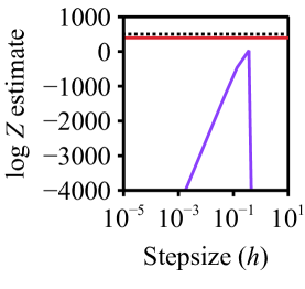
(a)

(b)

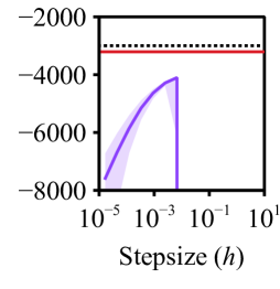
(c)

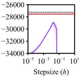
(d)

(e)

Figure 2: SMC-LMC with adaptive tuning v.s. fixed step sizes. The solid lines are the median estimate of $\log Z$, while the colored regions are the $80\%$ empirical quantiles computed over 32 replications.

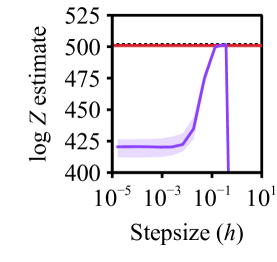
(a)

(b)

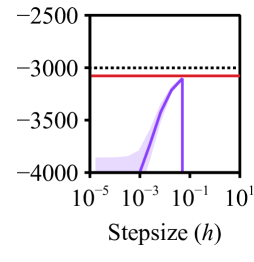
(c)

(d)

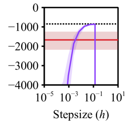
(e)

Figure 3: SMC-KLMC with adaptive tuning v.s. fixed step sizes and refreshment rates. For SMC-KLMC with fixed parameters $h,\rho$, we show the result of the best-performing refreshment rate. The solid lines are the median estimate of $\log Z$, while the colored regions are the $80\%$ empirical quantiles computed over 32 replications.

4.2 SMC with Kinetic Langevin Monte Carlo

Next, we consider a variant of the LMC that operates on the augmented state space $\mathcal{Z}=\mathcal{X}\times\mathcal{X}$, where, for $t\geq 0$, each state of the Feynman-Kac model is denoted as $\mathbold{z}_{t}=(\mathbold{x}_{t},\mathbold{v}_{t})\in\mathcal{Z}$, $\mathbold{x}_{t},\mathbold{v}_{t}\in\mathcal{X}$, $\mathcal{X}=\mathbb{R}^{d}$, and the target is

$$\pi_{t}^{\mathsf{klmc}}\left(\mathbold{x},\mathbold{v}\right)\triangleq\pi_{t}\left(\mathbold{x}\right)\mathcal{N}\left(\mathbold{v};\mathrm{0}_{d},\mathrm{I}_{d}\right)\,.$$

Evidently, the $\mathbold{x}$-marginal of the augmented target is $\pi$. Therefore, a Feynman-Kac model targeting $\pi_{t}^{\mathsf{klmc}}$ is also targeting $\pi$ by design. Kinetic Langevin Monte Carlo (KLMC; Horowitz, 1991; Duane et al., 1987), also commonly referred to as underdamped Langevin, is given by the SDE

$$\mathrm{d}\mathsfit{x}_{s} =\mathsfit{v}_{s}\mathrm{d}s$$

$$\mathrm{d}\mathsfit{v}_{s} =\nabla\log\pi\left(\mathsfit{v}_{s}\right)\mathrm{d}s-\eta\mathsfit{v}_{s}\mathrm{d}s+\sqrt{2\eta}\,\mathrm{d}B_{s}\,,$$

where $\eta>0$ is a tunable parameter called damping coefficient. The stationary distribution of the joint process ${(\mathsfit{x}_{s},\mathsfit{v})}_{v\geq 0}$ is then $\pi^{\mathsf{klmc}}$. This continuous time process corresponds to the “Nesterov acceleration (Nesterov, 1983; Su et al., 2016)” of Eq. 11 (Ma et al., 2021), meaning that the process should converge faster. We thus expect KLMC to reduce the required number of steps $T$ compared to LMC.

To simulate this, we consider the OBABO discretization (Leimkuhler & Matthews, 2013), which operates in a Gibbs scheme (Geman & Geman, 1984): its kernel

$$K_{t}\left(\mathbold{z}_{t-1},\mathrm{d}\mathbold{z}_{t}\right)$$

$$\;=R^{\rho}\left(\mathbold{v}_{t-1},\mathrm{d}\mathbold{v}_{t-\nicefrac{{1}}{{2}}}\right)S_{t}^{h,L}\left(\left(\mathbold{x}_{t-1},\mathbold{v}_{t-\nicefrac{{1}}{{2}}}\right),\left(\mathrm{d}\mathbold{x}_{t},\mathrm{d}\mathbold{v}_{t}\right)\right)$$

is a composition of the momentum refreshment kernel

$$R^{\rho}\left(\mathbold{v}_{t-1},\mathrm{d}\mathbold{v}_{t-\nicefrac{{1}}{{2}}}\right)\triangleq\mathcal{N}\left(\mathrm{d}\mathbold{v}_{t-\nicefrac{{1}}{{2}}};\;\sqrt{1-\rho^{2}}\,\mathbold{v}_{t-1},\rho^{2}\,\mathrm{I}_{d}\right)\,,$$

where $\rho\triangleq 1-\exp\left(-\eta h\right)\in(0,1)$ is the “momentum refreshment rate” for some step size $h>0$, and the Leapfrog integrator kernel

$$S^{h}_{t}\left(\left(\mathbold{x}_{t-1},\mathbold{v}_{t-\nicefrac{{1}}{{2}}}\right),\cdot\right)\triangleq\delta_{\Phi_{h,t}\left(\mathbold{x}_{t-1},\mathbold{v}_{t-\nicefrac{{1}}{{2}}}\right)}\left(\cdot\right)\,,$$

where $\Phi_{h,t}$ is a single step of leapfrog integration with step size $h$ preserving the “Hamiltonian energy” $-\log\pi_{t}^{\mathsf{klmc}}$. This discretization also coincides with the unadjusted version of the generalized Hamiltonian Monte Carlo algorithm (Duane et al., 1987; Neal, 2011) with a single leapfrog step.

Backward Kernel.

Since the kernel $S^{h_{t}}$ is a deterministic mapping, $K_{t}^{\theta_{t}}$ does not admit a density with respect to the Lebesgue measure. Therefore, we are restricted to a specific backward kernel that satisfies the condition in Eq. 3: Since the leapfrog integrator $\Phi_{h,t}$ is a diffeomorphism, its inverse map $\Phi_{h,t}^{-1}$ exists and can be easily simulated. Therefore, the choice of backward kernel

$$L_{t-1}^{h,\rho}\left(\mathbold{z}_{t},\cdot\right)=\delta_{\Phi_{h,t}^{-1}\left(\mathbold{x}_{t},\mathbold{v}_{t}\right)}\left(\left(\mathrm{d}\mathbold{x}_{t},\mathrm{d}\mathbold{v}_{t-\nicefrac{{1}}{{2}}}\right)\right)R^{\rho}\left(\mathbold{v}_{t-\nicefrac{{1}}{{2}}},\mathrm{d}\mathbold{v}_{t-1}\right)$$

ensures that the deterministic mapping is supported on the same pair of points, ensuring absolute continuity (Doucet et al., 2022; Geffner & Domke, 2023). Then,

$$G_{t}^{h_{t},\rho_{t}}\left(\mathbold{z}_{t-1},\mathbold{z}_{t}\right)$$

$$=\frac{\gamma_{t}\left(\mathbold{x}_{t}\right)\mathcal{N}\left(\mathbold{v}_{t};0_{d},\mathrm{I}_{d}\right)\mathcal{N}\left(\mathbold{v}_{t-1};\sqrt{1-\rho_{t}^{2}}\,\mathbold{v}_{t-\nicefrac{{1}}{{2}}},\rho_{t}^{2}\,\mathrm{I}_{d}\right)}{\gamma_{t-1}\left(\mathbold{x}_{t-1}\right)\mathcal{N}\left(\mathbold{v}_{t-1};0_{d},\mathrm{I}_{d}\right)\mathcal{N}\left(\mathbold{v}_{t-\nicefrac{{1}}{{2}}};\sqrt{1-\rho_{t}^{2}}\,\mathbold{v}_{t-1},\rho_{t}^{2}\mathrm{I}_{d}\right)}\,,$$

with two tunable parameters: $(h_{t},\rho_{t})\in\mathbb{R}_{>0}\times(0,1)$.

Figure 4: Distribution of tuned refreshment rates $\rho_{t}$. The results were obtained by running adaptive SMC on the Sonar problem with $T=256$ and $N=1024$

Adaptation Algorithm.

As KLMC has two parameters, we cannot immediately apply the tuning procedure offered in § 3.3. Thus, we will tailor it to KLMC. At each iteration $t\in[T]$, we will minimize the incremental KL objective $\widehat{\mathcal{L}}_{t}\left(h,\rho\right)$ through coordinate descent. That is, we alternate between minimizing over $h$ and $\rho$. This is shown in Alg. 3. In particular, $h_{t}$ is updated using the procedure used in § 3.3, while $\rho_{t}$ is directly minimized over a grid $\Xi\in{(0,1)}^{k}$ of $k$ grid points. As shown in Fig. 4, empirically, the minimizers of $\widehat{\mathcal{L}}_{t}$ with respect to $\rho_{t}$ tend to concentrate on the boundary, as if the adaptation problem is determining “to fully refresh” or “not refresh at all.” Therefore, the grid $\Xi$ can be made as coarse as $\Xi=\left\{0.1,0.9\right\}$, which is what we use in the experiments, with minimal impact.

5 Experiments

5.1 Implementation and General Setup

We implemented our SMC sampler using the Julia language (Bezanson et al., 2017). For resampling, we use the Srinivasan sampling process (SSP) by Gerber et al. (2019), which performs similarly to the popular systematic resampling strategy (Carpenter et al., 1999; Kitagawa, 1996), while having stronger theoretical guarantees. Resampling is triggered adaptively, which has theoretically shown to work well by Syed et al. (2024), under the typical rule of resampling as soon as the effective sample size (Kong, 1992; Elvira et al., 2022) goes below $\nicefrac{{N}}{{2}}$. In all cases, the reference distribution $q$ is a standard Gaussian as $q=\mathcal{N}\left(0_{d},\mathrm{I}_{d}\right)$, while we use quadratic annealing schedule $\lambda_{t}={\left(t/T\right)}^{2}$.

Evaluation Metric.

We will compare the estimate $\log\widehat{\mathsfit{Z}}_{T,N}$, where, for unbiased estimates of $Z$ against a ground truth estimate obtained by running a large budget run with $N=2^{14}$ and $T=2^{9}$. Due to adaptivity, our method only yields biased estimates of $Z$. Therefore, after adaptation, we run vanilla SMC with the tuned parameters, which yields unbiased estimates.

Benchmark Problems.

For the benchmarks, we ported some problems from the Inference Gym (Sountsov et al., 2020) to Julia, where the rest of the problems are taken from PosteriorDB (Magnusson et al., 2025). Details on the problems considered in this work are in App. A, while the configuration of our adaptive method is specified in App. B.

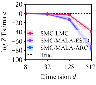
(a)

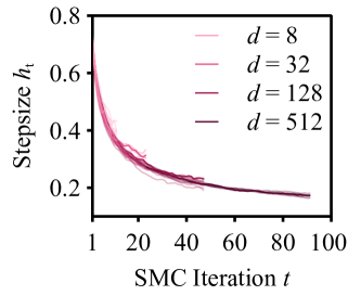
(b)

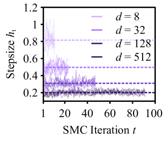
(c)

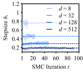
(d)

Figure 5: Dimensional scaling of adaptive SMC with Langevin-based kernels with (MALA) and without (LMC) MH adjustment. (a) Comparison of the $\log Z$ estimates under growing dimensionality. The solid lines are the median, while the shaded regions are the $80\%$ quantiles obtained from 32 replications. (b-d) Tuned step size schedules obtained under each sampler. SMC-MALA-ESJD uses ESJD maximization for adaptation, while SMC-MALA-ARC uses acceptance rate control (ARC). Each solid line is a step size schedule obtained from a single run (eight examples are shown), while the dotted lines of the MH-adjusted kernels are the average of the step sizes.

5.2 Comparison Against Fixed Step Sizes

Setup.

First, we evaluate the quality of the parameters tuned through our method. For this, we compare the performance of SMC-LMC and SMC-KLMC against hand tuning a fixed step size $h$, such that $h_{t}=h$, over a grid of step sizes. For KLMC, we also perform a grid search of the refreshment rate over $\{0.1,0.5,0.9\}$. The computational budgets are set as $N=1024$, $B=128$, and $T=64$.

Results.

A representative subset of the results is shown in Figs. 2 and 3, while the full set of results is shown in § F.1. First, we can see that SMC with fixed step sizes is strongly affected by tuning. On the other hand, our adaptive sampler obtains estimates that are closer or comparable to the best fixed step size on 20 out of 21 benchmark problems. Our method performed poorly on the Rats problem, which is shown in the right-most panes in Figs. 2 and 3. Overall, our method results in estimates that are better or comparable to those obtained with the best fixed step size.

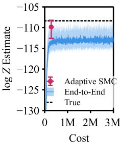
(a)

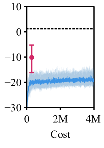
(b)

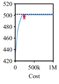
(c)

Figure 6: Comparison against end-to-end optimization. The “cost” is the cumulative number of gradient evaluations of the target. 32 independent runs for end-to-end optimization are shown. The error bars on adaptive SMC are $80\%$ empirical quantiles of the cost and the estimate computed from 32 replications.

5.3 Comparison Against End-to-End Optimization

Setup.

Now, we compare our adaptive tuning strategy against end-to-end optimization strategies. In particular, we compare against differentiable AIS (Geffner & Domke, 2023, 2021; Zhang et al., 2021) instead of SMC, as differentiating through resampling does not necessarily improve the results (Zenn & Bamler, 2023). To only evaluate the tuning capabilities, we do not optimize the reference $q$. However, results with reference tuning can be found in § F.2. Furthermore, we performed a grid-search over the SGD step sizes $\{10^{-4},10^{-3},10^{-2}\}$, and show the best results. Additional implementation details can be found in § B.2. Since end-to-end methods need to differentiate through the models, we only ran them on the problems with JAX (Bradbury et al., 2018) implementations (Funnel, Sonar, Brownian, and Pines). We use $T=32$ SMC iterations for all methods. For adaptation, our method uses $B=128$ particles out of $N=1024$ particles, while end-to-end optimization uses an SMC sampler with $32$ particles during optimization, and $N=1024$ particles when actually estimating $\widehat{\mathsfit{Z}}_{T,N}$. For both methods, the cost of estimating the unbiased normalizing constant is excluded.

Results.

The results are shown in Fig. 6. Our Adaptive SMC sampler achieves more accurate estimates than the best-tuned end-to-end tuning results on Sonar and Brownian. Therefore, we conclude that our SMC tuning approach achieves estimates that are better or on par with those obtained through end-to-end optimization.

5.4 Dimensional Scaling with and without Metropolis-Hastings Adjustment

We will now compare the tuned performance of unadjusted versus adjusted kernels, in particular, LMC versus MALA. To maintain a non-zero acceptance rate, MH-adjusted methods generally require $h$ to decrease with dimensionality $d$. Theoretical results suggest that, for MALA, the step size has to decrease as $\mathcal{O}\left(d^{-1/3}\right)$ (Chewi et al., 2021; Roberts & Tweedie, 1996) for Gaussian targets and as $\mathcal{O}\left(d^{-1/2}\right)$ in general (Chewi et al., 2021; Wu et al., 2022). In contrast, LMC only needs to reduce $h$ to counteract the asymptotic bias in the stationary distribution, which grows as $\mathcal{O}\left(d\right)$ in squared Wasserstein distance (Dalalyan, 2017; Durmus & Eberle, 2024; Durmus & Moulines, 2019). However, since SMC never operates in the stationary regime (except for the waste-free variant by Dau & Chopin 2022), we expect SMC-LMC to scale better than SMC-MALA with dimensionality $d$. Here, we will empirically verify this intuition.

Setup.

We set $\pi=\mathcal{N}\left(3\cdot 1_{d},\mathrm{I}_{d}\right)$ and $q=\mathcal{N}\left(0_{d},\mathrm{I}_{d}\right)$ under varying dimensionality $d$. The computational budgets are set as $N=1024$, $T=4\lceil\sqrt{d}\rceil$, where the latter is suggested by Syed et al. (2024, §4.7). For MALA, we will consider two common adaptation strategies: controlling the acceptance rate such that it is $0.575$ (Roberts & Tweedie, 1996) as done by Buchholz et al. (2021) and maximizing the ESJD (Pasarica & Gelman, 2010), as done by Buchholz et al. (2021); Fearnhead & Taylor (2013). For both, we use the tricks stated in § 3.2, such as subsampling and SAA, and the optimization algorithm in § 3.3.

Results.

The results are shown in Fig. 5, where we can see that the tuned stepsize of SMC-LMC is not affected by dimensionality whatsoever (Fig. 5(b)). In contrast, the MALA step sizes decrease as $d$ increases for both EJSD maximization and acceptance rate control (Figs. 5(c) and 5(d)); the scaling of the stepsize is close to the theoretical rate $h=\mathcal{O}(d^{-1/3})$. Consequently, SMC-ULA obtains more accurate estimates of the normalizing constant in higher dimensions (Fig. 5(a)). This demonstrates the fact that unadjusted kernels are effective when used in SMC.

6 Conclusions

In this work, we established a methodology for tuning path proposal kernels in SMC samplers, which involves greedily minimizing an incremental KL divergence at each SMC step. We developed a specific instantiation of the methodology for tuning scalar-valued step sizes in SMC samplers. Possible future directions include investigating the consistency of the proposed adaptation scheme, possibly through the framework of Beskos et al. (2016).

Appendix A Benchmark Problems

Name	Description	$d$	Source	Reference
Funnel	Neal’s funnel distribution.	10	Inference Gym	Sountsov et al. 2020 Neal 2003
Brownian	Latent Brownian motion with missing observations.	32	Inference Gym	Sountsov et al. 2020
Sonar	Bayesian logistic regression with the sonar classification dataset.	61	Inference Gym	Sountsov et al. 2020 Gorman & Sejnowski 1988
Pines	Log-Gaussian Cox process model of the concentration of Scotch pine saplings in Finland over a $40\times 40$ grid.	1600	Inference Gym	Sountsov et al. 2020 Møller et al. 1998

Table 1: Overview of Benchmark Problems

Name	Description	$d$	Source	References
Bones	Latent trait model for multiple ordered categorical response for quantifying skeletal maturity from radiograph maturity ratings with missing entries. (model: $\mathtt{bones\_model}$; dataset: $\mathtt{bones\_data}$)	13	PosteriorDB	Magnusson et al. 2025 Spiegelhalter et al. 1996
Surgical	Binomial regression model for estimating the mortality rate of pediatric cardiac surgery. (model: $\mathtt{surgical\_model}$; dataset: $\mathtt{surgical\_data}$)	14	PosteriorDB	Magnusson et al. 2025 Spiegelhalter et al. 1996
HMM	Hidden Markov model with a Gaussian emission on a simulated dataset. (model: $\mathtt{hmm\_gaussian}$; dataset: $\mathtt{hmm\_gaussian\_simulated}$)	14	PosteriorDB	Magnusson et al. 2022 Cappé et al. 2005
Loss Curves	Loss model of insurance claims. The model is the single line-of-business, single insurer (SISLOB) variant, where the dataset is the “ppauto” line of business, part of the “Schedule P loss data” provided by the Casualty Actuarial Society. (model: $\mathtt{losscurve\_sislob}$; dataset: $\mathtt{loss\_curves}$)	15	PosteriorDB	Magnusson et al. 2025 Cooney 2017
Pilots	Linear mixed effects model with varying intercepts for estimating the psychological effect of pilots when performing flight simulations on various airports. (model: $\mathtt{pilots}$; dataset: $\mathtt{pilots}$)	18	PosteriorDB	Magnusson et al. 2025 Gelman & Hill 2007
Diamonds	Log-log regression model for the price of diamonds with highly correlated predictors. (model: $\mathtt{diamonds}$; dataset: $\mathtt{diamonds}$)	26	PosteriorDB	Magnusson et al. 2025 Wickham 2016
Seeds	Random effect logistic regression model of the seed germination proportion of seeds from different root extracts. We use the variant with a half-Cauchy prior on the scale. (model: $\mathtt{seeds\_stanified\_model}$; dataset: $\mathtt{seeds\_data}$)	26	PosteriorDB	Magnusson et al. 2025 Crowder 1978 Spiegelhalter et al. 1996
Rats	Linear mixed effects model with varying slope and intercepts for modeling the weight of young rats over five weeks. (model: $\mathtt{rats\_model}$; data: $\mathtt{rats\_data}$)	65	PosteriorDB	Magnusson et al. 2025 Spiegelhalter et al. 1996 Gelfand et al. 1990
Radon	Multilevel mixed effects model with log-normal likelihood and varying intercepts for modeling the radon level measured in U.S. households. We use the Minnesota state subset. (model: $\mathtt{radon\_hierarchical\_intercept\_centered}$; dataset: $\mathtt{radon\_mn}$)	90	PosteriorDB	Magnusson et al. 2025 Gelman et al. 2014
Election88	Generalized linear mixed effects model of the voting outcome of individuals at the 1988 U.S. presidential election. (model: $\mathtt{election88\_full}$; dataset: $\mathtt{election88}$)	90	PosteriorDB	Magnusson et al. 2025 Gelman & Hill 2007

Table 2: Overview of Benchmark Problems

Name	Description	$d$	Source	Reference
Butterfly	Multispecies occupancy model with correlation between sites. The dataset contains counts of butterflies from twenty grassland sites in south-central Sweden (model: $\mathtt{butterfly}$; dataset: $\mathtt{multi\_occupancy}$)	106	PosteriorDB	Magnusson et al. 2025 Dorazio et al. 2006
Birds	Mixed effects model with a Poisson likelihood and varying intercepts for modeling the occupancy of the Coal tit (Parus ater) bird species during the breeding season in Switzerland. (model: $\mathtt{GLMM1\_model}$; dataset: $\mathtt{GLMM\_data}$)	237	PosteriorDB	Magnusson et al. 2025 Kéry & Schaub 2012
Drivers	Time series model with seasonal effects of driving-related fatalities and serious injuries in the U.K. from Jan. 1969 to Dec. 1984. (model: $\mathtt{state\_space\_stochastic\_level\_stochastic\_seasonal}$; dataset: $\mathtt{uk\_drivers}$)	389	PosteriorDB	Magnusson et al. 2025 Commandeur & Koopman 2007
Capture	Model of capture-recapture data for estimating the population size. This is the “heterogeneity model,” where the detection probability is assumed to be heterogeneous across the individuals. The data is simulated. (model: $\mathtt{Mh\_model}$; dataset: $\mathtt{Mh\_data}$)	388	PosteriorDB	Magnusson et al. 2025 Kéry & Schaub 2012
Science	Item response model with generalized rating scale. The dataset was taken from the Consumer Protection and Perceptions of Science and Technology section of the 1992 Euro-Barometer Survey. (model: $\mathtt{grsm\_latent\_reg\_irt}$; dataset: $\mathtt{science\_irt}$)	408	PosteriorDB	Magnusson et al. 2025 Reif & Melich 1993 Furr 2017
Three Men	Latent Dirichlet allocation for topic modeling. The number of topics is set as $K=2$, while the dataset is corpus 2 among pre-processed multilingual corpora of the book “Three Men and a Boat.” (model: $\mathtt{ldaK2}$; dataset: $\mathtt{three\_men3}$)	505	PosteriorDB	Magnusson et al. 2025 Farkas 2014 Blei et al. 2003
TIMSS	Item response model with generalized partial credit. The dataset is from the TIMSS 2011 mathematics assessment of Australian and Taiwanese students. (model: $\mathtt{gpcm\_latent\_reg\_irt}$; dataset: $\mathtt{timssAusTwn\_irt}$)	530	PosteriorDB	Magnusson et al. 2025 Muraki 1997 Mullis et al. 2012

Table 3: Overview of Benchmark Problems

In this section, we provide additional details about the benchmark problems. A full list of the problems is shown in Tables 1, 2 and 3. For the problems we ported from the Inference Gym, we provide additional details for clarity:

Funnel.

This is the classic benchmark problem by Neal (2003). We use the formulation:

$$y \sim\mathcal{N}\left(0,3^{2}\right)$$

$$x \sim\mathcal{N}\left(0_{d-1},e^{y}\mathrm{I}_{d-1}\right)\,,$$

where $d=10$.

Sonar.

This is a logistic regression problem with a standard normal prior on the coefficients. That is, given a dataset $(X,y)$, where $X\in\mathbb{R}^{n,d-1}$ and $y\in\mathbb{R}^{n}$,

$$\beta \sim\mathcal{N}\left(0_{d},\mathrm{I}_{d}\right)$$

$$y \sim\mathrm{Bernoulli}\left(\sigma\left(X\beta\right)\right)\,,$$

where $\sigma\left(x\right)\triangleq 1/\left(1+\mathrm{e}^{-x}\right)$ is the logistic function. Here, we use the sonar classification dataset by Gorman & Sejnowski (1988). The features are pre-processed with $z$-standardization following Phillips et al. (2024).

Pines.

This is a log-Gaussian Cox process (LGCP; Møller et al., 1998) model applied to a dataset of Scotch pine samplings in Finland as described in (Møller et al., 1998). An LGCP is a nonparametric model of intensity fields, where the observations are assumed to follow a Poisson point process. Consider a 2-dimensional grid of $n$ cells indexed by $i\in[n]$, each denoted by $S_{i}\in\mathcal{S}$ and centered on the location $x_{i}\in\mathbb{R}^{d}$. The dataset is the number of points contained in the $i$th cell, $y_{i}\in\mathbb{N}_{\geq 0}$, for all $i\in[n]$, which is assumed to follow a Poisson point process

$$y_{i}\sim\mathrm{Poisson}\left(\int_{S_{i}}\lambda\left(x\right)\mathrm{d}x\right)\,,$$

given the intensity field

$$\log\lambda\sim\mathcal{GP}\left(\mu,k\right)\,,$$

where $\mathcal{GP}\left(\mu,k\right)$ is a Gaussian process prior (GP; Rasmussen & Williams, 2005) with mean $\mu$ and covariance kernel $k:\mathbb{R}^{2}\times\mathbb{R}^{2}\to\mathbb{R}_{>0}$. In our case, we use the grid approximation

$$\int_{S_{i}}\lambda\left(x\right)\mathrm{d}x\approx A_{i}\exp\left(\log\lambda\left(x_{i}\right)\right)\,,$$

where $A_{i}$ is the area of $S_{i}$. The likelihood is then

$$\ell\left(y_{i},x_{i},\lambda\right)=\exp\left\{\lambda\left(\mathbold{x}_{i}\right)y_{i}-A_{i}\exp\left(\lambda\left(\mathbold{x}_{i}\right)\right)\right\}\,.$$

Following Møller et al. (1998), the hyperparameters of the GP are set as

$$\mu =\log\left(126\right)-\frac{\sigma^{2}}{2}$$

$$k\left(\mathbold{x}_{i},\mathbold{x}_{j}\right) =\sigma^{2}\exp\left(-\frac{{\left\lVert\mathbold{x}_{i}-\mathbold{x}_{j}\right\rVert}_{2}}{\sqrt{{\left|\mathcal{S}\right|}\beta^{2}}}\right)\,,$$

where

$$\sigma^{2}=1.91\quad\text{and}\quad\beta=\frac{1}{33}\,.$$

The field $[0,1]^{2}$ is discretized into a $40\times 40$ grid such that ${\left|\mathcal{S}\right|}=40^{2}$ and $A_{i}=1/{\left|\mathcal{S}\right|}$. Furthermore, to improve the conditioning of the posterior, we apply whitening of the GP prior (Murray & Adams, 2010, §2.1).

Appendix B Details on the Experimental Setup

B.1 Setup of Adaptive SMC Samplers

Configuration of the Adaptation Procedure.

Here, we collected the specification of the tunable parameters in our adaptive SMC samplers. The parameters in SMC-LMC are set as in Table 4:

Name	Source	Value
$\tau$	§ 3.2	0.1
$\epsilon$	Alg. 5	0.01
$c$	Alg. 6	0.1
$r$	Alg. 6	2
$\delta$	Alg. 4	$-1$
$h_{\mathsf{guess}}$	Alg. 4	$\exp\left(-10\right)\approx 4.54\times 10^{-5}$

Table 4: Configuration of SMC-LMC

The parameters in SMC-KLMC are set as in Table 5:

Name	Source	Value
$\tau$	§ 3.2	5
$\epsilon$	Alg. 5	$0.01$
$c$	Alg. 6	$0.01$
$r$	Alg. 6	3
$\delta$	Alg. 4	$-1$
$\Xi$	Alg. 3	$\{0.1,0.9\}$
$\rho_{\mathsf{guess}}$	Alg. 3	$0.1$
$h_{\mathsf{guess}}$	Alg. 4	$\exp\left(-7.5\right)\approx 5.53\times 10^{-4}$

Table 5: Configuration of SMC-KLMC

Schedule Adaptation.

In some of the experiments, we evaluate the performance of our step size adaptation procedure when combined with an annealing temperature schedule (${(\lambda_{t})}_{t=0,\ldots,T}$) adaptation scheme. In particular, we use the recently proposed method of Syed et al. (2024), which is able to tune both the schedule ${(\lambda_{t})}_{t=0,\ldots,T}$ and the number of SMC steps $T$. Under regularity assumptions, the resulting adaptation schedule asymptotically ($N\to\infty$ and $T\to\infty$) approximates the optimal geometric annealing path that minimizes the variance of the normalizing constant estimator. For a detailed description, see Syed et al. (2024, Sec. 5). Below, we provide a concise introduction to the schedule adaptation process.

Syed et al. (2024, §4.3) demonstrate that, under suitable regularity assumptions, the asymptotically optimal schedule is the one that achieves a “local communication barrier”

$$\text{LCB}(\lambda_{t-1},\lambda_{t})\approx\sqrt{\mathrm{R}(\pi_{t-1}\otimes K_{t}^{\mathbold{\theta}}||\pi_{t}\otimes L_{t-1}^{\mathbold{\theta}})},$$

that is uniform across all adjacent steps $\lambda_{t},\lambda_{t-1}$ for all $t\in[T]$. As such, the corresponding adaptation scheme estimates the local communication barrier and uses it to obtain a temperature schedule that makes it uniform. Intuitively, $\text{LCB}(\lambda_{t-1},\lambda_{t})$ quantifies the “difficulty” of approximating $\pi_{t}\otimes L_{t-1}^{\mathbold{\theta}}$ using weighted particles drawn from $\pi_{t-1}\otimes K_{t}^{\mathbold{\theta}}$.

In addition, let us denote the local communication barrier accumulated up to time step $t\in\{0,\ldots,T\}$,

$$\Lambda(\lambda_{t})\triangleq\sum_{s=1}^{t}\text{LCB}(\lambda_{t-1},\lambda_{t})\;.$$

This serves as a divergence measure for the “length” of the annealing path from $\lambda_{0}=0$ to $\lambda_{t}$. Furthermore, the total accumulated local barrier

$$\Lambda\triangleq\Lambda(\lambda_{T})\;,$$

which is referred to as the global communication barrier, quantifies the total difficulty of simulating the annealing path ${(\pi_{t})}_{t\in\{0,\ldots,T\}}$. Syed et al. (2024) show that for the normalizing constant to be accurate, SMC needs to operate in what they call the “stable discretization regime,” which occurs at $T=\mathrm{O}\left(\Lambda\right)$. Therefore, for tuning the number of SMC steps, a good heuristic is setting $T$ to be a constant multiple of the estimated global communication barrier.

The corresponding schedule adaptation scheme is as follows: From the estimates of the communication barrier ${(\widehat{\Lambda}\left(\lambda_{t}\right))}_{t\in[T]}$ obtained from a previous run, the updated schedule for the next run of length $T^{\prime}$ is set via mapping

$$\lambda_{t}^{\star}=\widehat{\Lambda}_{\text{inv}}\left(\widehat{\Lambda}\times\frac{t}{T^{\prime}}\right),\quad t^{\prime}=0,\dots,T^{\prime},$$

where the inverse mapping $\widehat{\Lambda}_{\text{inv}}$ is approximated using a monotonic spline with knots $\{(\widehat{\Lambda}(\lambda_{t}),\lambda_{t})\}_{t=0}^{T}$. In our case, the length of the new schedule is set as $T^{\prime}=2\widehat{\Lambda}$.

Below, we summarize the general steps for adaptive SMC with round-based schedule adaptation:

1. Run Adaptive SMC with $T_{r}$ and $r=1$.

2. Using the statistics generated during 1, adapt the schedule using the method of Syed et al. (2024) to

   $$T_{r}=2\widehat{\Lambda}$$

3. Run SMC with $T_{r}$ and the adapted schedule.

4. Set $r\leftarrow r+1$ and go to step ❷.

B.2 Setup of End-to-End Optimization

We provide additional implementation details for end-to-end optimization. We implemented two differentiable AIS methods: one based on LMC (Thin et al., 2021) and another based on KLMC (Geffner & Domke, 2021; Doucet et al., 2022). Both methods are implemented in JAX (Bradbury et al., 2018), modified from the code provided by Geffner & Domke (2023).

For optimization, we used the Adam optimizer (Kingma & Ba, 2015) with three different learning rates $\{10^{-4},10^{-3},10^{-2}\}$ for $5{,}000$ iterations, with a batch size of $32$. We evaluated two different annealing step sizes ($32$ and $64$), keeping the number of steps fixed during training while optimizing the annealing schedule (detailed in § F.2). Each setting was repeated $32$ times, and we report results from the best-performing configurations.

Following the setup in (Doucet et al., 2022), the step size is learned through a function $\epsilon_{\theta}(t):[0,1]\to\mathbb{R}^{d}$ (d is the dimension of the target dsitribution). This function is parameterized as a 2-layer fully connected neural network with 32 hidden units and ReLU activation, followed by a scaled sigmoid function which constrains $\epsilon_{\theta}(t)<0.1$ for the ULA variant and constrain $\epsilon_{\theta}(t)<0.25$ for UHA variant. We find that enforcing these step size constraints is necessary to prevent numerical issues during training, which was acknowledged in prior works (Doucet et al., 2022; Geffner & Domke, 2021).

For schedule adaptation, Doucet et al. (2022); Geffner & Domke (2021), parameterize the temperature schedule as

$$\lambda_{t}=\frac{\sum_{t^{\prime}\leq t}\sigma\left(b_{t^{\prime}}\right)}{\sum_{t^{\prime}=1}^{T}\sigma\left(b_{t^{\prime}}\right)}\,,$$

where $\sigma$ is the sigmoid function, $\lambda_{0}$ is fixed to be 0, and $b_{0:T-1}$ is subject to optimization. We additionally learn the momentum refreshment rate $\rho$ (shared across $t\in[T]$) for DSMC-UHA, that is parametrized with a parameter $u$ as $\rho=.98\sigma(u)+.01$ to ensure $\rho\in(0.01,0.99)$, following the identical setting from Doucet et al. (2022).

Appendix C Algorithms

In this section, we will provide a detailed description of our proposed adaptation algorithms and their components.

C.1 $\mathtt{FindFeasible}$ (Algorithm 4)

Input: Objective $f:\mathbb{R}\to\mathbb{R}$,
initial guess $x_{0}\in\mathbb{R}$,
backing off stepsize $\delta\in\mathbb{R}\setminus\{0\}$.

Output: Feasible initial point $x_{0}$

1 $x\leftarrow x_{0}$

2 while  $f\left(x\right)=\infty$ do

3    $x\leftarrow x+\delta$

4   

5 end while

Return $x$

Algorithm 4 $\mathtt{FindFeasible}\left(f,x_{0},\Delta\right)$

Although our algorithms are capable of operating in numerically unstable regions, it is computationally convenient to initialize on a numerically stable region. When the user provides a guess, we take a conservative approach of not assuming that it is on a numerically non-degenerate region. As such, we must first check that it is non-degenerate, and if it is not, we must move it to somewhere that is. This is done by $\mathtt{FindFeasible}\left(f,x_{0},\delta\right)$ shown in Alg. 4. If $x_{0}$ is already feasible, it immediately returns the initial point $x_{0}$. Otherwise, if $x_{0}$ is degenerate, it increases or decreases $x_{0}$ with a stepsize of $\delta$ until the function becomes feasible.

C.2 $\mathtt{GoldenSectionSearch}$ (Alg. 5)

Input: Objective $f:\mathbb{R}\to\mathbb{R}\cup\{\infty\}$,
initial triplet $(a,b,c)$ satisfying Eq. 13,
absolute tolerance $\epsilon$.

1 $\phi^{-1}\triangleq\nicefrac{{\left(\sqrt{5}-1\right)}}{{2}}$

2 $x_{0}\leftarrow a$

3 $x_{3}\leftarrow c$

4 if  ${\left|c-b\right|}>{\left|b-a\right|}$  then

5    $x_{1}\leftarrow b$

6    $x_{2}\leftarrow b+\left(1-\phi^{-1}\right)\left(c-b\right)$

7   

8else

9    $x_{2}\leftarrow b$

10    $x_{1}\leftarrow b-\left(1-\phi^{-1}\right)\left(b-a\right)$

11   

12 end if

13$f_{1}\leftarrow f\left(x_{1}\right)$

14 $f_{2}\leftarrow f\left(x_{2}\right)$

15 while  ${\left|x_{1}-x_{2}\right|}>\epsilon/2$  do

16    if  $f_{2}<f_{1}$  then

17       $x_{0}\leftarrow x_{1}$

18       $x_{1}\leftarrow x_{2}$

19       $x_{2}\leftarrow\phi^{-1}x_{2}+\left(1-\phi^{-1}\right)x_{3}$

20       $f_{1}\leftarrow f_{2}$

21       $f_{2}\leftarrow f\left(x_{2}\right)$

22      

23   else

24       $x_{3}\leftarrow x_{2}$

25       $x_{2}\leftarrow x_{1}$

26       $x_{1}\leftarrow\phi^{-1}x_{1}+\left(1-\phi^{-1}\right)x_{0}$

27       $f_{2}\leftarrow f_{1}$

28       $f_{1}\leftarrow f\left(x_{1}\right)$

29      

30    end if

31   

32 end while

33if If $f_{1}\leq f_{2}$ then

34    Return $x_{1}$

35   

36else

37    Return $x_{2}$

38   

39 end if

Algorithm 5 $\mathtt{GoldenSectionSearch}\left(f,a,b,c,\epsilon\right)$

The workhorse of our stepsize adaptation scheme is the golden section search (GSS) algorithm by Avriel & Wilde (1968), which is a variation of the Fibonacci search algorithm by Kiefer (1953). In particular, we are using the implementation of Press et al. (1992, §10.1), shown in Alg. 5, which uses a triplet, $(a,b,c)$, for initialization. This triplet requires the condition

$$a<b<c,\quad f\left(b\right)<f\left(a\right),\;\text{and}\;f\left(b\right)<f\left(c\right)$$ (12)

to hold. Then, by Lemma 1, this implies that the closed interval $[a,c]$ contains a local minimum, which need not be close to $b$. Then, GSS is guaranteed to find a local minimum at a “linear rate” of $\nicefrac{{\left(1-\sqrt{5}\right)}}{{2}}\approx 1.62$, the golden ratio, resulting in a query/iteration complexity of $\mathcal{O}\left(\log{\left|c-a\right|}/\epsilon\right)$. Furthermore, if $f$ is unimodal (Assumption 2), then the solution will be $\epsilon$-close to the global minimum (Luenberger & Ye, 2008, §7.1). The key is to find a valid triplet $(a,b,c)$, which is done in Alg. 6 that will follow.

Input: Objective $f:\mathbb{R}\to\mathbb{R}\cup\{\infty\}$,
initial point $x_{0}\in(-\infty,x^{\infty})$,
exponential search coefficient $c>0$,
exponential search base $r>1$.

Output: Triplet $(x^{-},x_{\mathsf{mid}},x^{+})$

1 $x\leftarrow x_{0}$

2 $y\leftarrow f(x)$

3 $k\leftarrow 0$

4 while  true  do

5    $x^{\prime}\leftarrow x_{0}+cr^{k}$

6    $y^{\prime}\leftarrow f\left(x^{\prime}\right)$

7    if  $y<y^{\prime}$ then

8       $x^{+}\leftarrow x^{\prime}$

9       $x_{0}\leftarrow x$

10       break

11      

12    end if

13   $x\leftarrow x^{\prime}$

14    $y\leftarrow y^{\prime}$

15    $k\leftarrow k+1$

16   

17 end while

18$k\leftarrow 0$

19 while  true  do

20    $x^{\prime}\leftarrow x_{0}-cr^{k}$

21    $y^{\prime}\leftarrow f\left(x^{\prime}\right)$

22    if  $y<y^{\prime}$ then

23       $x^{-}\leftarrow x^{\prime}$

24       $x_{\mathsf{mid}}\leftarrow x$

25       break

26      

27    end if

28   $x\leftarrow x^{\prime}$

29    $y\leftarrow y^{\prime}$

30    $k\leftarrow k+1$

31   

32 end while

Return $(x^{-},x_{\mathsf{mid}},x^{+})$

Algorithm 6 $\mathtt{BracketMinimum}\left(f,x_{0},c,r\right)$

C.3 $\mathtt{BracketMinimum}$ (Algorithm 6)

The main difficulty of applying GSS in practice is setting the initial bracketing interval. If the bracketing interval does not contain a local minimum, nothing can be said about what GSS is converging towards. In our case, we require a triplet $(a,b,c)$ that satisfies the sufficient conditions in Lemma 2. Therefore, an algorithm for finding such an interval is necessary. Naturally, this algorithm should have a computational cost that is better or at least comparable to GSS. Otherwise, a more naive way of setting the intervals would make more sense. Furthermore, the width of the interval found by the algorithm should be as narrow as possible so that GSS can be run more efficiently.

While Press et al. (1992, §10.1) presents an algorithm for finding such a bracket using parabolic interpolation, the efficiency and output quality of this algorithm are not analyzed. Furthermore, the presence of discontinuities in our objective function (Assumption 3) warrants a simpler algorithm that is provably robust. Therefore, we use a specialized routine, $\mathtt{BracketMinimum}$, shown in Alg. 6.

$\mathtt{BracketMinimum}$ works in two stages: Given an initial point $x_{0}$, it expands the search interval to the right (towards $+\infty$; Line 5-23) and then to the left (towards $-\infty$; Line 25-36). During this, it generates a sequence of exponentially increasing intervals (Lines 7 and 25) and, in the second stage, stops when it detects points that satisfy the condition in Equation 13. This algorithm was inspired by a Stack Exchange post by Lavrov (2017), which was in turn inspired by the exponential search algorithm (Bentley & Yao, 1976).

The bulk of the tunable parameters of the adaptation method described in § 3.3 comes from $\mathtt{BracketMinimum}$. In fact, the parameters of $\mathtt{BracketMinimum}$ most crucially affect the overall computational performance of our schemes. Recall that the convergence of GSS depends on the width of the provided triplet, ${\left|a-c\right|}$. Given, this $c$ and $r$ affect computational performance through the following: (a) The width of the resulting triplet, ${\left|a-c\right|}$, increases with $r$ and $c$. (b) Smaller $r$ and $c$ requires more time to find a valid triplet.

C.4 $\mathtt{Minimize}$ (Algorithm 7)

Input: objective $f:\mathbb{R}\to\mathbb{R}\cup\{\infty\}$,
initial point $x_{0}\in\mathbb{R}$ such that $f\left(x_{0}\right)<\infty$,
minimum search coefficient $c\in\mathbb{R}\setminus\{0\}$,
minimum search exponent $r>1$,
absolute tolerance $\epsilon>0$.

1 $(x^{-},x_{\mathsf{int}},x^{+})\leftarrow\mathtt{BracketMinimum}\left(f,x_{0},+c,r\right)$

$x^{*}\leftarrow\mathtt{GoldenSectionSearch}\left(f,\,x^{-},\,x_{\mathsf{int}},\,x^{+},\epsilon\right)$

Algorithm 7 $\mathtt{Minimize}\left(f,x_{0},c,r,\epsilon\right)$

We finally discuss our complete optimization routine, which is shown in Alg. 7. Given an initial point $x_{0}$ and suitable assumptions, $\mathtt{Minimize}\left(f,x_{0},c,r,\epsilon\right)$ finds a point that is $\epsilon$-close to a local minimum. This is done by first finding an interval that contains the minimum (Line 1) by calling $\mathtt{BracketMinimum}$, which is then used by $\mathtt{GoldenSectionSearch}$ for proper optimization (Line 2). As such, the computation cost of the routine is the sum of the two stages.

There are four parameters: $x_{0},c,r,\epsilon$. Admissible values of $\epsilon$ will depend on the requirements of the downstream task. On the other hand, $c$ and $r$ can be optimized. The effect of these parameters on the execution time is analyzed in Theorem 1, while a discussion on how to interpret the theoretical analysis is in § 3.4.

Appendix D Theoretical Analysis

In this section, we will provide a formal theoretical analysis of the algorithms presented in App. C as well as the omitted proof of the theorems in the main text.

D.1 Definitions and Assumptions

Formally, when we say “local minimum,” we follow the following definition:

Definition 1 (Definition 7; Rudin, 1976).

Consider some continuous function $f:\mathcal{X}\to\mathbb{R}$ on a metric space $\mathcal{X}\subseteq\mathbb{R}$. We say $f$ has a local minimum at $x^{*}\in\mathcal{X}$ if there exists some $\epsilon>0$ such that $f\left(x^{*}\right)\leq f\left(x\right)$ for all $x\in\mathcal{X}$ with ${\left|x^{*}-x\right|}<\epsilon$ .

Also, unimodal functions are defined as follows:

Definition 2.

We say $f:[a,b]\to\mathbb{R}$ is unimodal if there exists some point $x^{*}$ such that $f$ is monotonically strictly decreasing on $[a,x^{*}]$ and strictly increasing on $[x^{*},b]$.

Now, recall that our adaptation objective in § 3.2 operates on $\mathbb{R}_{>0}$. During adaptation, however, the objectives are log-transformed so that optimization is performed on $\mathbb{R}$. Therefore, it is convenient to assume everything happens on $\mathbb{R}$. That is, instead of Assumption 1 and 2, we will work with the following assumptions that are equivalent up to log transformation:

Assumption 3.

For the objective $f:\mathbb{R}\to\mathbb{R}\cup\{\infty\}$, we assume the following:

1. There exists some $x^{\infty}\in(-\infty,\infty]$ such that $x$ is finite and continuous on $(-\infty,x^{\infty})$ and $\infty$ on $[x^{\infty},\infty)$.

2. There exists some $\underline{x}\in(-\infty,x^{\infty})$ such that $f$ is strictly monotonically decreasing on $(-\infty,\underline{x}]$.

3. There exists some $\overline{x}\in[\underline{x},x^{\infty})$ such that $f$ is strictly monotonically increasing on $[\overline{x},x^{\infty})$

Assumption 4.

$f$ is unimodal on $(-\infty,x^{\infty})$.

Evidently, these assumptions are equivalent to Assumption 1 and 2 by setting

$$f\left(x\right) =\mathcal{L}\left(\exp\left(x\right)\right)$$

$$\overline{x} =\log\overline{h}$$

$$\underline{x} =\log\underline{h}$$

$$x^{\infty} =\log h^{\infty}\,.$$

D.2 Proof of § 3.1

[pathdivergence]

D.3 Sufficient Condition for an Interval to Contain a Local Minimum (Lemma 1)

Our adaptation algorithms primarily rely on GSS (Algorithm 5) to identify a local optimum. To guarantee this, however, GSS needs to be initialized on an interval that contains a local minimum. For this, the following lemma establishes a sufficient condition for identifying such intervals. As such, we will use these conditions as invariants during the execution of GSS, such that it finds narrower and narrower intervals that continue to contain a local minimum.

Lemma 1.

Let $f$ satisfy Assumption 3. Suppose that there exist some $a<b<c$ such that

$$f\left(b\right)\leq f\left(a\right)<\infty\quad\text{and}\quad f\left(b\right)\leq f\left(c\right)\,.$$ (13)

Then $(a,c)$ contains a local minimum of $f$ on $(-\infty,x^{\infty})$.

Proof.

Consider any triplet $(a^{\prime},b^{\prime},c^{\prime})$ consisting of three points $a^{\prime}<b^{\prime}<c^{\prime}$ with $f(b^{\prime})\leq f(a^{\prime})<\infty$ and $f(b^{\prime})\leq f(c^{\prime})<\infty$. Then $(a^{\prime},c^{\prime})$ contains a local minimum of $f$: $f$ attains its minimum on $[a^{\prime},c^{\prime}]$ by the extreme value theorem, which is either on $(a^{\prime},c^{\prime})$—in which case the result holds immediately—or on $\{a^{\prime},c^{\prime}\}$—in which case the result holds because $b^{\prime}$ is a local minimum since $f(b^{\prime})\leq\min\{f(a^{\prime}),f(c^{\prime})\}$.

We now apply this result to triplets contained in $[a,c]$. First, if $c<x^{\infty}$, use the triplet $(a^{\prime},b^{\prime},c^{\prime})=(a,b,c)$. For the remaining cases, assume $c\geq x^{\infty}$. If $b\geq\overline{x}$, set the triplet $(a^{\prime},b^{\prime},c^{\prime})=(a,b,d)$ for any $d\in(b,x^{\infty})$. If $b<\overline{x}$ and $f(\overline{x})\geq f(b)$, set the triplet $(a^{\prime},b^{\prime},c^{\prime})=(a,b,\overline{x})$. Otherwise, if $b<\overline{x}$ and $f(\overline{x})<f(b)$, set the triplet $(a^{\prime},b^{\prime},c^{\prime})=(b,\overline{x},d)$ for any $d\in(\overline{x},x^{\infty})$. ∎

D.4 $\mathtt{GoldenSectionSearch}$ (Lemma 2)

We first establish that, under suitable initialization, GSS is able to locate a local minimum. Most existing results assume that $f$ is unimodal (Luenberger & Ye, 2008, §7.1) and show that GSS converges to the unique global minimum. Here, we prove a more general result that holds under weaker conditions: GSS can also find a local minimum even when unimodality doesn’t hold. For this, we establish that our assumptions in Assumption 3 and initializing at a triplet $(a,b,c)$ satisfying the condition in Lemma 1 are sufficient. Furthermore, while it is well known that GSS achieves a linear convergence rate with coefficient $\phi\triangleq(1+\sqrt{5})/2$, we could not find a proof that exactly applied to the GSS variant by Press et al. (1992), which is the one we use. Therefore, we also prove linear convergence rate with a proof that precisely applies to Algorithm 5.

Lemma 2.

Suppose Assumption 3 holds. Then, for any triplet $(a,b,c)$ satisfying $a<b<c$, $f(b)\leq f(a)<\infty$, and $f(b)\leq f(c)$, $\mathtt{GoldenSectionSearch}\left(f,a,b,c,\epsilon\right)$ returns a point $x^{*}\in(-\infty,x^{\infty})$ that is $\epsilon$-close to a local minimum after

$$\mathrm{\Theta}\left(\log{\left|c-a\right|}\frac{1}{\epsilon}\right)$$

objective evaluations, where $\phi=\left(1+\sqrt{5}\right)/2$.

Proof.

For clarity, let us denote the value of the variables $x_{0},x_{1},x_{2},x_{3}$ set at iteration $k\geq 1$ of the while loop in Line 13-27 as $x_{0}^{k},x_{1}^{k},x_{2}^{k},x_{3}^{k}$. Before the while loop at $k=0$, they are initialized as follows: If ${\left|c-b\right|}\geq{\left|b-a\right|}$,

$$\left(x_{0}^{0},\;x_{1}^{0},\;x_{2}^{0},\;x_{3}^{0}\right)=\left(a,\;b,\;b+\left(1-\phi^{-1}\right)\left(c-b\right),\;c\right)$$

and

$$\left(x_{0}^{0},\;x_{1}^{0},\;x_{2}^{0},\;x_{3}^{0}\right)=\left(a,\;b+\left(1-\phi^{-1}\right)\left(b-a\right),\;b,\;c\right)$$

otherwise. For all $k\geq 0$, the following set of variables are set as follows: If $f\left(x_{2}^{k}\right)<f\left(x_{1}^{k}\right)$, the next set of variables are set as

$$\left(x_{0}^{k+1},\;x_{1}^{k+1},\;x_{2}^{k+1},\;x_{3}^{k+1}\right)$$

$$\qquad\triangleq\left(x_{1}^{k},\;x_{2}^{k},\;\phi^{-1}x_{2}^{k}+\left(1-\phi^{-1}\right)x_{3}^{k},\;x_{3}^{k}\right)\,,$$ (14)

and

$$(x_{0}^{k+1},\,x_{1}^{k+1},\,x_{2}^{k+1},\,x_{3}^{k+1})$$

$$\qquad\triangleq(x_{0}^{k},\,\phi^{-1}x_{1}^{k}+\left(1-\phi^{-1}\right)x_{0}^{k},\,x_{1}^{k},\,x_{2}^{k})$$

otherwise. We also denote $f_{2}^{k}\triangleq f\left(x_{2}^{k}\right)$ and $f_{1}^{k}\triangleq f\left(x_{1}^{k}\right)$.

Assuming the algorithm terminates at some $k^{*}<\infty$, the algorithm outputs either $x_{1}^{k^{*}}$ or $x_{2}^{k^{*}}$. Therefore, it suffice to show that $k^{*}<\infty$, ${\left|x_{2}^{k^{*}}-x_{1}^{k^{*}}\right|}\leq\epsilon/2$, and that the interval $(x_{0}^{k^{*}},x_{3}^{k^{*}})$ contains a local minimum.

First, let’s establish that $k^{*}<\infty$. GSS terminates as soon as ${\left|x_{3}^{k}-x_{0}^{k}\right|}\leq\epsilon$ for some $0\geq k<\infty$. We will establish this by showing that ${\left|x_{3}^{k}-x_{0}^{k}\right|}$ satisfies a contraction. For this, however, we first have to show that $x_{1}^{k},x_{2}^{k}$ satisfy

$$x_{1}^{k} =\phi^{-1}x_{0}^{k}+\left(1-\phi^{-1}\right)x_{3}^{k}$$ (15)

$$x_{2}^{k} =\left(1-\phi^{-1}\right)x_{0}^{k}+\phi^{-1}x_{3}^{k}$$ (16)

at all $k\geq 0$. We will show this via induction. Before we proceed, notice that the name “golden” section search comes from the fact that $\phi$, the golden ratio, is the solution to the equation

$$\phi^{2}=\phi+1\quad\Rightarrow\quad 1-\phi^{-1}=\phi^{-2}\,.$$ (17)

Now, for some $k>0$, suppose Equations 15 and 16 hold. Then, if $f_{2}^{k}<f_{1}^{k}$,

$$x_{1}^{k+1} =x_{2}^{k}$$

$$=\left(1-\phi^{-1}\right)x_{0}^{k}+\phi^{-1}x_{3}^{k},$$

$$=\phi^{-2}x_{0}^{k}+\left(1-\phi^{-2}\right)x_{3}^{k}$$ (Eq. 17)

$$=\phi^{-2}x_{0}^{k}+\left(1+\phi^{-1}\right)\left(1-\phi^{-1}\right)x_{3}^{k}$$

$$=\phi^{-1}\left(\phi^{-1}x_{0}^{k}+\left(1-\phi^{-1}\right)x_{3}^{k}\right)$$

$$\qquad\qquad+\left(1-\phi^{-1}\right)x_{3}^{k}\,,$$

$$=\phi^{-1}x_{1}^{k}+\left(1-\phi^{-1}\right)x_{3}^{k}$$ (Eq. 15)

$$=\phi^{-1}x_{0}^{k+1}+\left(1-\phi^{-1}\right)x_{3}^{k+1}\,.$$ (Eq. 20)

This establishes Equation 15 for $k+1$. Similarly,

$$x_{2}^{k+1} =\phi^{-1}x_{2}^{k}+\left(1-\phi^{-1}\right)x_{3}^{k}\,,$$

$$=\phi^{-1}\left(\left(1-\phi^{-1}\right)x_{0}^{k}+\phi^{-1}x_{3}^{k}\right)$$

$$\qquad\qquad+{\left(1-\phi^{-1}\right)}x_{3}^{k}$$ (Eq. 16)

$$=\phi^{-1}\left(1-\phi^{-1}\right)x_{0}^{k}$$

$$\qquad\qquad+{\left(1-\phi^{-1}+\phi^{-2}\right)}x_{3}^{k}$$

$$=\left(1-\phi^{-1}\right)\left(\phi^{-1}x_{0}^{k}+\left(1-\phi^{-1}\right)x_{3}^{k}\right)$$

$$\qquad\qquad+\phi^{-1}x_{3}^{k}\,,$$

$$=\left(1-\phi^{-1}\right)x_{1}^{k}+\phi^{-1}x_{3}^{k+1}$$ (Eq. 15)

$$=\left(1-\phi^{-1}\right)x_{0}^{k+1}+\phi^{-1}x_{3}^{k+1}\,.$$ (Eq. 20)

This establishes Equation 16 for $k+1$. The proof for the remaining case of $f_{2}^{k}\geq f_{1}^{k}$ is identical due to symmetry. Furthermore, the base case for $k=0$ automatically holds due to the condition on $(a,b,c)$. Therefore, Equations 15 and 16 hold for all $k\geq 0$.

From Equations 15 and 16, we now have a precise rate of decrease for the interval ${\left|x_{3}^{k}-x_{0}^{k}\right|}$. That is, for $f_{2}^{k}<f_{1}^{k}$,

$${\left|x_{3}^{k}-x_{0}^{k}\right|} ={\left|x_{3}^{k-1}-x_{1}^{k-1}\right|}$$

$$={\left|x_{3}^{k-1}-\left(\phi^{-1}x_{0}^{k-1}+\left(1-\phi^{-1}\right)x_{3}^{k-1}\right)\right|}$$

$$=\phi^{-1}{\left|x_{3}^{k-1}-x_{0}^{k-1}\right|}\,$$

and for $f_{2}^{k}\geq f_{1}^{k}$,

$${\left|x_{3}^{k}-x_{0}^{k}\right|} ={\left|x_{2}^{k-1}-x_{0}^{k-1}\right|}$$

$$={\left|\left(\left(1-\phi^{-1}\right)x_{0}^{k-1}+\phi^{-1}x_{3}^{k-1}\right)-x_{0}^{k-1}\right|}$$

$$=\phi^{-1}{\left|x_{3}^{k-1}-x_{0}^{k-1}\right|}\,.$$

Furthermore, This implies, for all $k\geq 1$, the interval $[x_{3}^{k},x_{0}^{k}]$ shrinks at a geometrical rate

$${\left|x_{3}^{k}-x_{0}^{k}\right|}=\phi^{-k}{\left|x_{3}^{0}-x_{0}^{0}\right|}\,.$$

Then,

$${\left|x_{2}^{k}-x_{1}^{k}\right|} =\left(2\phi^{-1}-1\right){\left|x_{0}^{k}-x_{3}^{k}\right|}\leq\epsilon/2$$

can be guaranteed by iterating until the smallest iteration count $k\geq 1$ that satisfies

$$\phi^{-k}{\left|x_{3}^{0}-x_{0}^{0}\right|}\leq\frac{1}{2\phi^{-1}-1}\,\frac{\epsilon}{2}\,,$$

$$k=\left\lceil\frac{1}{\log\phi}\log\frac{2\left(2\phi^{-1}-1\right){\left|c-a\right|}}{\epsilon}\right\rceil\,,$$

which yields the execution time complexity statement.

We now prove that the interval $(x_{0}^{k^{*}},x_{0}^{k^{*}})$ contains a local minima. For this, we will prove a stronger result that $(x_{0}^{k},x_{3}^{k})$ contains a local minimum for all $k\geq 0$ by induction. Suppose, for some $k\geq 1$,

$$\min\left(f_{1}^{k},f_{2}^{k}\right) \leq f(x_{0}^{k})<\infty$$ (18)

$$\min\left(f_{1}^{k},f_{2}^{k}\right) \leq f(x_{3}^{k})$$ (19)

hold. If $f_{2}^{k}<f_{1}^{k}$, the next set of variables are set as

$$(x_{0}^{k+1},x_{1}^{k+1},x_{3}^{k+1})=(x_{1}^{k},x_{2}^{k},x_{3}^{k})\,,$$ (20)

which guarantees that the inequalities

$$\min\left(f_{1}^{k+1},f_{2}^{k+1}\right) \leq f_{1}^{k+1}=f_{2}^{k}\leq f(x_{0}^{k+1})<\infty$$

$$\min\left(f_{1}^{k+1},f_{2}^{k+1}\right) \leq f_{1}^{k+1}=f_{2}^{k}\leq f(x_{3}^{k+1})$$

hold. Otherwise, if $f_{2}^{k}\geq f_{1}^{k}$,

$$(x_{0}^{k+1},x_{2}^{k+1},x_{3}^{k+1})=(x_{0}^{k},x_{1}^{k},x_{2}^{k})\,,$$

guarantee

$$\min\left(f_{1}^{k+1},f_{2}^{k+1}\right) \leq f_{2}^{k+1}=f_{1}^{k}\leq f(x_{0}^{k+1})<\infty$$

$$\min\left(f_{1}^{k+1},f_{2}^{k+1}\right) \leq f_{2}^{k+1}=f_{1}^{k}\leq f(x_{3}^{k+1})\,.$$

The base case $k=0$ trivially holds by assumption $f(b)<f\left(x_{0}^{0}\right)<\infty$, $f(b)<f(x_{3}^{0})$, and the fact that either $x_{1}^{0}$ or $x_{2}^{0}$ is set as $b$. Therefore, Equations 18 and 19 hold for all $k\geq 0$. Equations 18 and 19 imply that either $(x_{0}^{k},x_{1}^{k},x_{3}^{k})$ or $(x_{0}^{k},x_{2}^{k},x_{3}^{k})$ satisfy the condition in Lemma 1. Therefore, a local minimum is contained in $(x_{0}^{k},x_{3}^{k})$ for all $k\geq 0$. ∎

D.5 $\mathtt{BracketMinimum}$ (Lemma 3)

We now prove that $\mathtt{BracketMinimum}$ returns a triplet $(x^{-},x_{\mathsf{mid}},x^{+})$ satisfying the condition in Lemma 1. Furthermore, under Assumption 3, we analyze the width of the initial search interval represented by the triplet, ${\left|x^{+}-x^{-}\right|}$. Note that, while $\mathtt{BracketMinimum}$ is designed to be valid even if $x_{0}\geq x^{\infty}$, accommodating this complicates the analysis. Therefore, in the analysis that will follow, we will assume $x_{0}<x^{\infty}$.

Lemma 3.

Suppose Assumption 3 holds. Then $\mathtt{BracketMinimum}\left(f,x_{0},r,c\right)$ for $x_{0}\in(-\infty,x^{\infty})$ returns a triplet $(x^{-},x_{\mathsf{mid}},x^{+})$, where $x^{-}<x_{\mathsf{mid}}<x^{+}$,

$$f\left(x_{\mathsf{mid}}\right)\leq f\left(x^{-}\right)<\infty,\quad f\left(x_{\mathsf{mid}}\right)\leq f\left(x^{+}\right),$$ (21)

and

$${\left|x^{+}-x^{-}\right|}\leq r^{2}\left((r+1)[\overline{x}-x_{0}]_{+}+[x_{0}-\underline{x}]_{+}\right)+3r^{2}c$$

after

$$\mathrm{O}\left\{{\left(\log r\right)}^{-1}\log_{+}\left((r[\overline{x}-x_{0}]_{+}+[x_{0}-\underline{x}]_{+})/c\right)\right\}$$

objective evaluations.

Proof.

$\mathtt{BracketMinimum}$ has two stages: exponential search to the right (Stage I) and exponential search to the left (Stage II). In the worst case, Stage I must pass $\overline{x}$ moving to the right starting from $x_{0}$, which takes at most $\mathrm{O}(\bar{k}_{r})$ iterations, where

$$\bar{k}_{r}=\left\lceil(\log r)^{-1}\log_{+}((\overline{x}-x_{0})/c)\right\rceil\;.$$

Similarly, in the worst case Stage II must pass $\underline{x}$ moving to the left starting from $x_{0}+cr^{\bar{k}_{r}}$, which takes at most $\mathrm{O}(\bar{k}_{\ell})$ iterations, where

$$\bar{k}_{\ell} =\left\lceil{\left(\log r\right)}^{-1}\log_{+}\left(\left(x_{0}+cr^{\bar{k}_{r}}-\underline{x}\right)/c\right)\right\rceil$$

$$\leq\left\lceil{\left(\log r\right)}^{-1}\log_{+}\left(x_{0}+\left(r{\left[\overline{x}-x_{0}\right]}_{+}-\underline{x}\right)/c\right)\right\rceil\,.$$

Adding these two costs yields the stated result. At the end of Stage I, by inspection, we know that $f(x)\leq f(x^{+})$, and that $f(x)<\infty$. Also, Stage II continues until the first increase in objective value, which guarantees that $\infty>f(x^{-})\geq f(x_{\text{mid}})$ and $f(x_{\text{mid}})\leq f(x)\leq f(x^{+})$. Finally,

$${\left|x^{+}-x^{-}\right|} \leq\left(x_{0}+cr^{\bar{k}_{r}+1}\right)-\left(x_{0}+cr^{\bar{k}_{r}}-cr^{\bar{k}_{\ell}+1}\right)$$

$$\leq rc\left(r^{\bar{k}_{r}}+r^{\bar{k}_{\ell}}\right)$$

$$\leq r\left(r[\overline{x}-x_{0}]_{+}+rc+r[x_{0}+cr^{\bar{k}_{r}}-\underline{x}]_{+}+rc\right)$$

$$\leq r^{2}\left([\overline{x}-x_{0}]_{+}+[x_{0}-\underline{x}]_{+}+cr^{\bar{k}_{r}}+2c\right)$$

$$\leq r^{2}\left([\overline{x}-x_{0}]_{+}+[x_{0}-\underline{x}]_{+}+r[\overline{x}-x_{0}]_{+}+3c\right)$$

$$=r^{2}\left((r+1)[\overline{x}-x_{0}]_{+}+[x_{0}-\underline{x}]_{+}\right)+3r^{2}c\;.$$

∎

D.6 $\mathtt{Minimize}$ (Theorem 1)

We prove that combining $\mathtt{BracketMinimum}$ and $\mathtt{GoldenSectionSearch}$, which we call $\mathtt{Minimize}$, results in an optimization algorithm that finds a point $\epsilon$-close to local minimum in $\mathrm{O}\left(\log\left(\Delta/\epsilon\right)\right)$ time.

Theorem 1.

Suppose Assumption 3 holds. Then, $\mathtt{Minimize}\left(f,x_{0},c,r,\epsilon\right)$ returns a point that is $\epsilon$-close to a local minimum after $\mathcal{C}_{\mathsf{bm}}+\mathcal{C}_{\mathsf{gss}}$ objective evaluations, where

$$\mathcal{C}_{\mathsf{bm}} =\mathrm{O}\left\{\frac{1}{\log r}\log_{+}\left(\Delta\frac{r}{c}\right)\right\}$$

$$\mathcal{C}_{\mathsf{gss}} =\mathrm{O}\left\{\log_{+}\left(r^{3}\Delta+r^{2}c\right)\frac{1}{\epsilon}\right\}\,,$$

where $\Delta\triangleq{\left[x_{0}-\underline{x}\right]}_{+}+{\left[\overline{x}-x_{0}\right]}_{+}\;.$

Proof.

$\mathcal{C}_{\mathsf{bm}}$ immediately follows from Lemma 3, while $\mathcal{C}_{\mathsf{gss}}$, on the other hand, follows from Lemma 2 as

$$\mathcal{C}_{\mathsf{gss}} =\mathrm{O}\left\{\log_{+}\left(x^{+}-x^{-}\right)\frac{1}{\epsilon}\right\}$$

$$=\mathrm{O}\left\{\log_{+}\left(r^{3}\Delta+r^{2}c\right)\frac{1}{\epsilon}\right\}\;,$$

where we plugged in the bound on ${\left|x^{+}-x^{-}\right|}$ from Lemma 3. This yields the stated result. Furthermore, since $\mathtt{BracketMinimum}$ returns a triplet $(x^{-},x_{\mathsf{mid}},x^{+})$ that satisfies the requirement of $\mathtt{GoldenSectionSearch}$ as stated in Lemma 2, the output $x^{*}\in(-\infty,x^{\infty})$ is $\epsilon$-close to a local minimum. ∎

Remark 1.

In Theorem 1, the “difficulty” of the problem is represented by $\Delta\geq 0$, where the magnitude of ${[x_{0}-\underline{x}]}_{+}$ and ${[\overline{x}-x_{0}]}_{+}$ represent the quality of the initialization $x_{0}$ (how much $x_{0}$ undershoots or overshoots $\overline{x}$ and $\underline{x}$). Furthermore, we have $\Delta\geq{\left|\overline{x}-\underline{x}\right|}$, where ${\left|\overline{x}-\underline{x}\right|}$ can be thought as the quantitative multimodality of the problem. Therefore, the execution time of $\mathtt{Minimize}$ becomes longer as the problem becomes more multimodal and the initialization is far from $[\overline{x},\underline{x}]$.

Remark 2.

The execution time of $\mathtt{Minimize}(f,x_{0},c,r,\epsilon)$ depends on $r$ and $c$. In general, the best-case performance ($\Delta=0$) can only become worse as $c$ increases. On the other hand, in the worst-case when $\Delta$ is large, increasing $r$ reduces $\mathcal{C}_{\mathsf{bm}}$, while slowly making $\mathcal{C}_{\mathrm{gss}}$ worse. Therefore, a large $r$ improves the worst-case performance.

D.7 $\mathtt{AdaptStepsize}$ (Proof of Assumption 1)

We now present the proof for the theoretical guarantees of Alg. 2 in the main text, Assumption 1. Since most of the heavy lifting in Alg. 2 is done by Alg. 7, Assumption 1 is almost a corollary of Theorem 1. The main difference is that Alg. 2 invokes Alg. 4 at $t=1$ and operates in log-space. Therefore, the proof incorporates these two modifications into the results of Theorem 1.

[initializestepsize]

Appendix E Backward Kernels

E.1 Some backward kernels are not like the others

Here, we would like to discuss some options for the “backward kernel” used in SMC samplers in the static model setting (Del Moral et al., 2006; Neal, 2001).

Detailed Balance Formula.

In the literature, the choice

$$L_{t-1}^{\mathsf{dbf}}\left(\mathbold{x}_{t},\mathbold{x}_{t-1}\right) \triangleq\frac{\gamma_{t}\left(\mathbold{x}_{t}\right)K_{t}\left(\mathbold{x}_{t-1},\mathbold{x}_{t}\right)}{\gamma_{t}\left(\mathbold{x}_{t-1}\right)}\,,$$ (22)

which we will refer to as the “detailed balance formula backward kernel,” has been the widely used (Dai et al., 2022; Bernton et al., 2019; Heng et al., 2020). The most convenient fact about Eq. 22 is that it results in a simple expression for the potential

$$G_{t}\left(\mathbold{x}_{t-1},\mathbold{x}_{t}\right)=\frac{\gamma_{t}\left(\mathbold{x}_{t-1}\right)}{\gamma_{t-1}\left(\mathbold{x}_{t-1}\right)}\,,$$

does not involve the densities of $K_{t}$. The origin of this backward kernel is that most $\pi_{t}$-invariant MCMC kernels used in practice satisfy the detailed balance formula (Robert & Casella, 2004, Def. 6.45) with $\pi_{t}$,

$$\pi_{t}\left(\mathbold{x}_{t-1}\right)K_{t}\left(\mathbold{x}_{t-1},\mathbold{x}_{t}\right)=\pi_{t}\left(\mathbold{x}_{t}\right)K_{t}\left(\mathbold{x}_{t},\mathbold{x}_{t-1}\right)\,,$$

which, given $L_{t-1}^{\mathsf{dbf}}\left(\mathbold{x}_{t-1},\mathbold{x}_{t}\right)=K_{t}\left(\mathbold{x}_{t-1},\mathbold{x}_{t}\right)$, yields Eq. 22 after re-aranging.

The detailed balance formula backward kernel is biased.

Now, let’s focus on the fact that $K_{t}=L_{t-1}^{\mathsf{dbf}}$ only holds under the detailed balance condition. Said differently, $L_{t-1}^{\mathsf{dbf}}$ is a properly normalized kernel only when $K_{t}$ satisfies detailed balance. This implies that, for non-reversible kernels like LMC, using the detailed balance formula kernel with $h>0$ may result in biased normalized constant estimates. This bias can be substantial, as we will see in § E.2. Fortunately, this bias does diminish as $h_{t}\to 0$ and $T\to\infty$ since the continuous Langevin dynamics is reversible under stationarity (Heng et al., 2020). However, the need for smaller step sizes means that a larger number of SMC steps $T$ has to be taken for the Markov process to converge.

Forward Kernel.

The properly normalized analog of $L^{\mathsf{dbf}}_{t-1}$ at time $t\geq 1$ is the “forward” kernel

$$L_{t-1}^{\mathsf{fwd}}\left(\mathbold{x}_{t},\mathbold{x}_{t-1}\right)\triangleq K_{t}\left(\mathbold{x}_{t},\mathbold{x}_{t-1}\right)\,.$$

This has been used, for example, by Thin et al. (2021). Recall that the “optimal” $L_{t-1}$ is a kernel that transports the particles following $P_{t}$ to follow $P_{t-1}$. The fact that we are using $K_{t}$ to do this implies that we are assuming $P_{t}\approx P_{t-1}$, which is only true if $T$ is large. We propose a different option, which should work even when $T$ is moderate or small.

Time-Correct Forward Kernel.

In § 4.1, we used the forward kernel at time $t-1$,

$$L_{t-1}^{\text{{tc-fwd}}}\left(\mathbold{x}_{t},\mathbold{x}_{t-1}\right)\triangleq K_{{\color[rgb]{.75,0,.25}t-1}}\left(\mathbold{x}_{t},\mathbold{x}_{t-1}\right)\,,$$

which we will refer to as the time-correct forward kernel. Unlike $L^{\mathsf{fwd}}_{t-1}$, the stationary distribution of this transport map is properly $\pi_{t-1}$. Informally, the reasoning is that

$$\frac{\left(\pi_{t}\otimes K_{t-1}\right)\left(x_{t},x_{t-1}\right)}{\left(\pi_{t-1}\otimes K_{t}\right)\left(x_{t-1},x_{t}\right)}\approx\frac{\left(\pi_{t}\otimes\pi_{t-1}\right)\left(x_{t},x_{t-1}\right)}{\left(\pi_{t-1}\otimes\pi_{t}\right)\left(x_{t-1},x_{t}\right)}=1\,.$$

Therefore, this should result in lower variance.

E.2 Empirical Evaluation

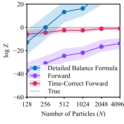
Figure 7: Comparison of backward kernels for SMC-LMC. The solid lines are the median, while the colored bands mark the $80\%$ empirical quantile over 256 replications.

Setup.

We compare the three backward kernels on a toy problem with $d=10$ dimensional Gaussians: $\pi=\mathcal{N}\left(30\cdot\mathrm{1}_{d},\mathrm{I}_{d}\right)$, $q_{0}=\mathcal{N}\left(0_{d},\mathrm{I}_{d}\right)$. Since the scale of the target distribution is constant under geometric annealing, a fixed stepsize $h=h_{t}=0.5$ should work well. We use a linear schedule with $T=64$.

Results.

The results are shown in Fig. 7. The backward kernel from the detailed balance formula severely overestimates the normalizing constant due to bias, while the forward kernel exhibits significantly higher variance than the time-correct forward kernel.

E.3 Conclusions

We have demonstrated that caution must be taken when using the popular backward kernel based on the detail-balance formula. Instead, we have proposed the “time-correct forward kernel,” which is not only valid but also results in substantially lower variance. Unfortunately, the time-correct forward kernel is only available for MCMC kernels that have a tractable density, which may not be the case; for instance, the KLMC kernel used in § 4.2 does not have this option. However, whenever it is available, it should be preferred.

Appendix F Additional Experimental Results

F.1 Comparison Against Fixed Stepsizes

F.1.1 SMC-LMC

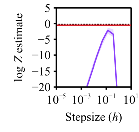
(a)

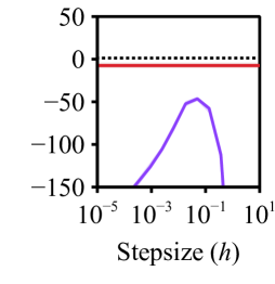
(b)

(c)

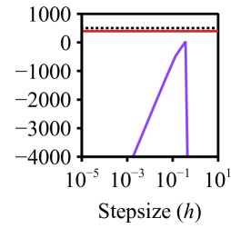
(d)

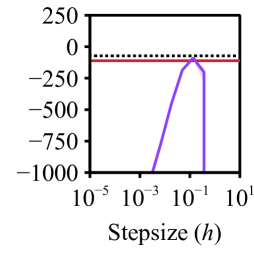
(e)

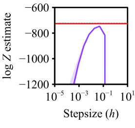
(f)

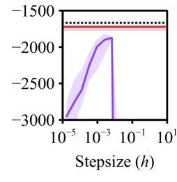
(g)

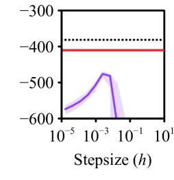
(h)

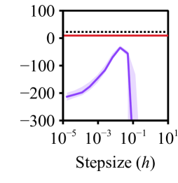
(i)

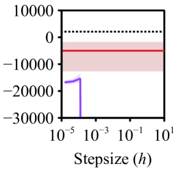
(j)

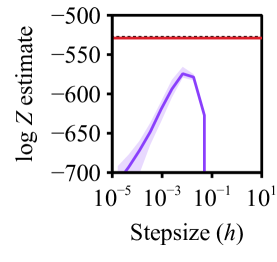
(k)

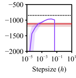
(l)

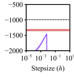
(m)

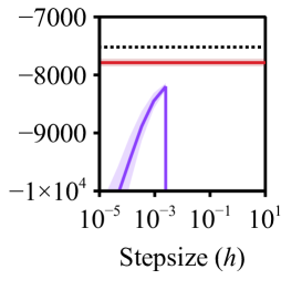
(n)

(o)

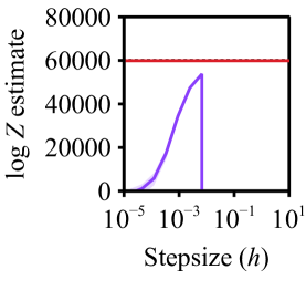
(p)

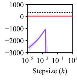
(q)

(r)

(s)

(t)

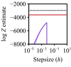
(u)

Figure 8: SMC-LMC with adaptive tuning v.s. fixed stepsizes. The solid lines are the median estimate of $\log Z$, while the colored regions are the $80\%$ empirical quantiles computed over 32 replications.

F.1.2 SMC-KLMC

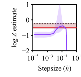
(a)

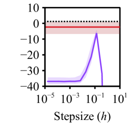
(b)

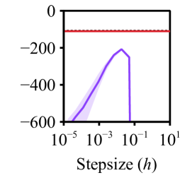
(c)

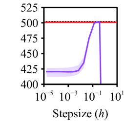
(d)

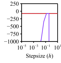
(e)

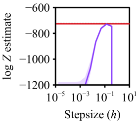
(f)

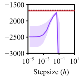
(g)

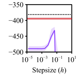
(h)

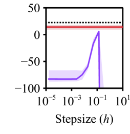
(i)

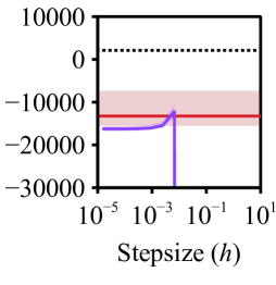
(j)

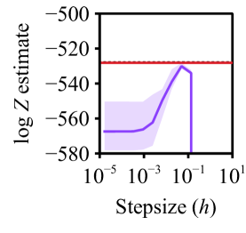
(k)

(l)

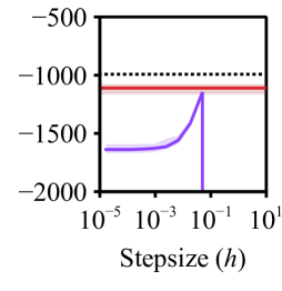
(m)

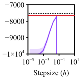
(n)

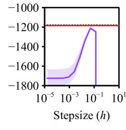
(o)

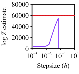
(p)

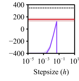
(q)

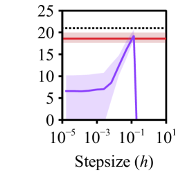
(r)

(s)

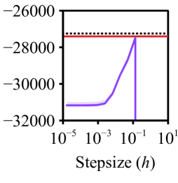
(t)

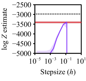
(u)

Figure 9: SMC-KLMC with adaptive tuning v.s. fixed stepsizes and refreshment rates. For SMC-KLMC with fixed parameters $h,\rho$, we show the result of the best-performing refreshment rate. The solid lines are the median estimate of $\log Z$, while the colored regions are the $80\%$ empirical quantiles computed over 32 replications.

F.2 Comparison Against End-to-End Optimization

F.2.1 SMC-LMC

For all results, the “cost” is calculated as the cumulative number of gradients and hessian evaluations used by each method. (End-to-end optimization methods require Hessians due to differentiating the gradient-based MCMC proposals.) For all figures, the error bars/bands are $80\%$ empirical quantiles computed from 32 replications, while $\gamma$ is the Adam stepsize used for end-to-end optimization.

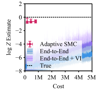
(a)

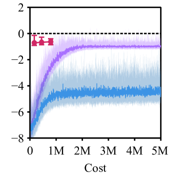
(b)

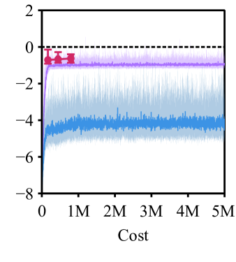
(c)

Figure 10: Comparison against end-to-end optimization on Funnel.

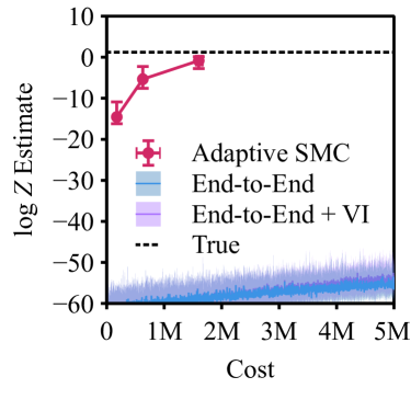
(a)

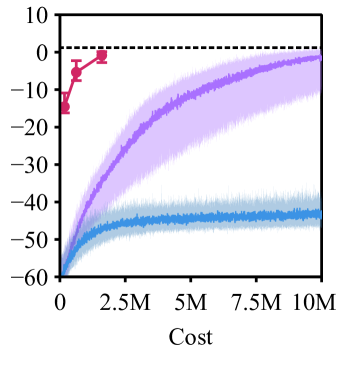
(b)

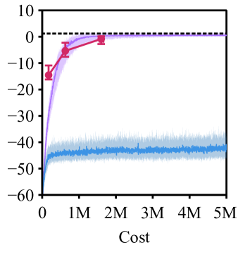
(c)

Figure 11: Comparison against end-to-end optimization on Brownian.

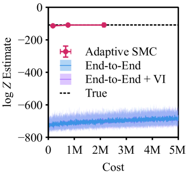
(a)

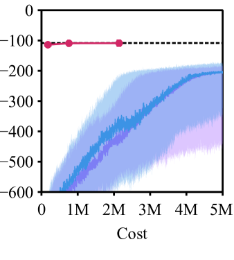
(b)

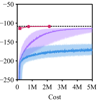
(c)

Figure 12: Comparison against end-to-end optimization on Sonar.

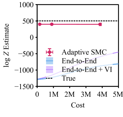
(a)

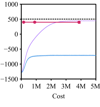
(b)

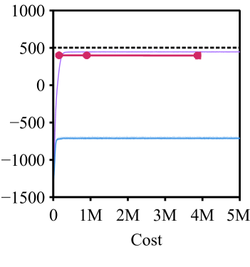
(c)

Figure 13: Comparison against end-to-end optimization Pines

F.2.2 SMC-KLMC

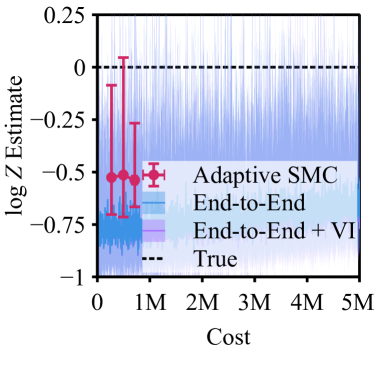
(a)

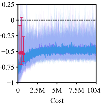
(b)

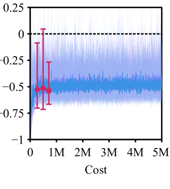
(c)

Figure 14: Comparison against end-to-end optimization on Funnel.

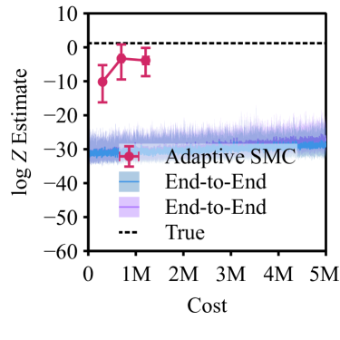
(a)

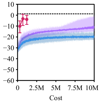
(b)

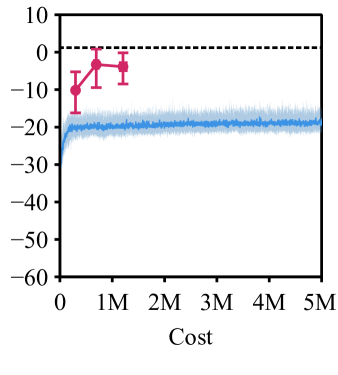
(c)

Figure 15: Comparison against end-to-end optimization on Brownian.

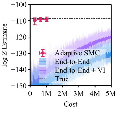
(a)

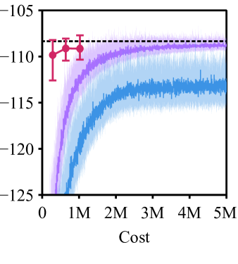
(b)

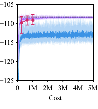
(c)

Figure 16: Comparison against end-to-end optimization on Sonar.

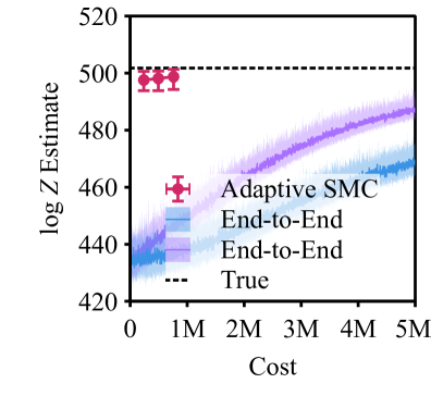
(a)

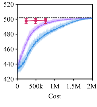
(b)

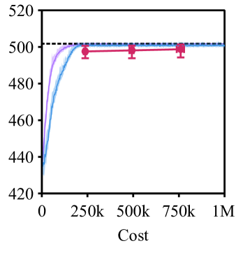
(c)

Figure 17: Comparison against end-to-end optimization on Pines.

F.3 Adaptation Cost

In this section, we will visualize the cost of adaptation of our algorithm. In particular, we show the number of objective evaluations used at each SMC iteration during adaptation. Recall that the cost of evaluating our objective is in the order of $\mathcal{O}\left(B\right)$ unnormalized log-density evaluations ($\log\gamma$) and its gradients ($\nabla\log\gamma$), where $B$ is the number of subsampled particles (§ 3.2). Therefore, the cost of $N/B$ adaptation objective evaluations at every SMC step roughly amounts to the cost of a single vanilla SMC run with $N$ particles. That is, for $N=1024$ and $B=128$, the cost of running our adaptive SMC sampler is comparable to two to three times that of a vanilla SMC sampler. The exact number of objective evaluations spent at each SMC iteration is shown in the figures that will follow. All experiments used $N=1024$, $B=128$, and $T=64$

F.3.1 SMC-LMC

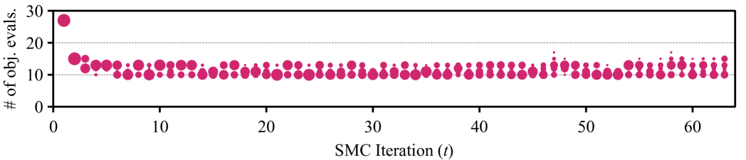
(a)

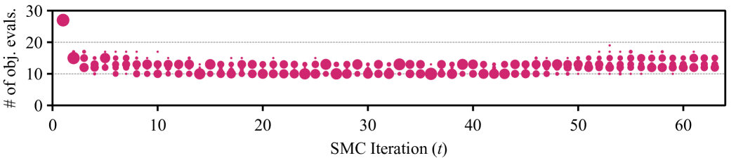
(b)

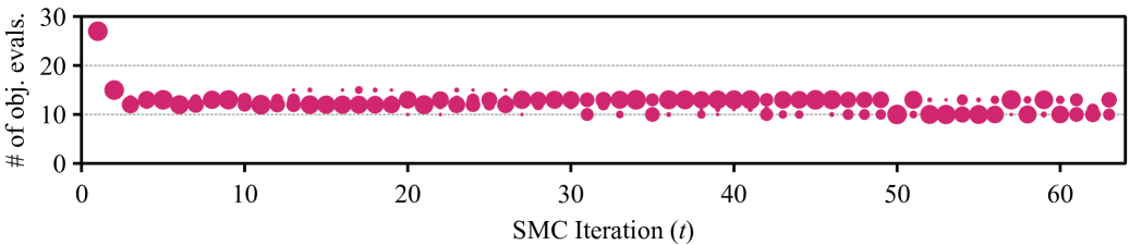
(c)

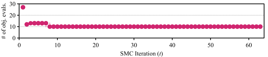
(d)

Figure 18: Number of objective evaluations spent during adaptation at each SMC iteration. The size of the markers represents the proportion of runs that spent each respective number of evaluations among 32 independent runs.

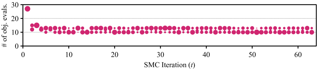
(a)

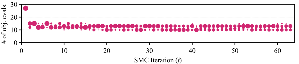
(b)

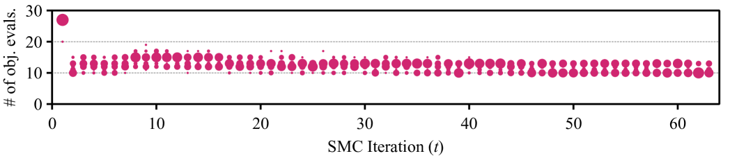
(c)

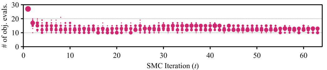
(d)

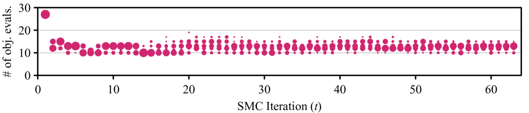
(e)

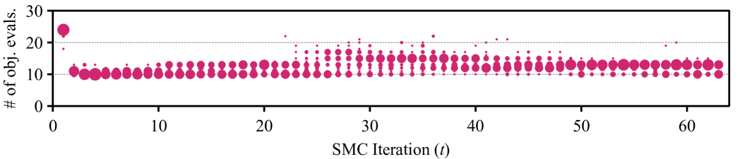
(f)

Figure 19: Number of objective evaluations spent during adaptation at each SMC iteration. The size of the markers represents the proportion of runs that spent each respective number of evaluations among 32 independent runs.

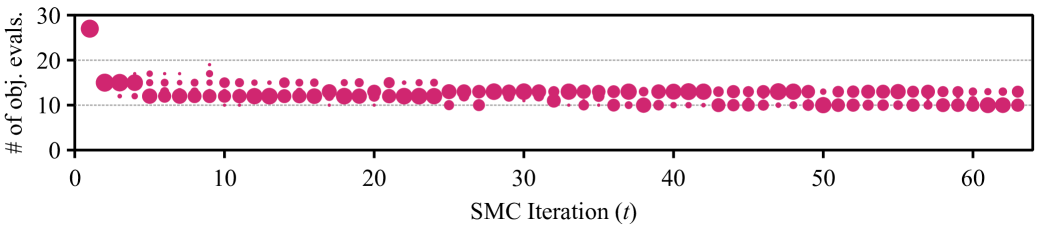
(a)

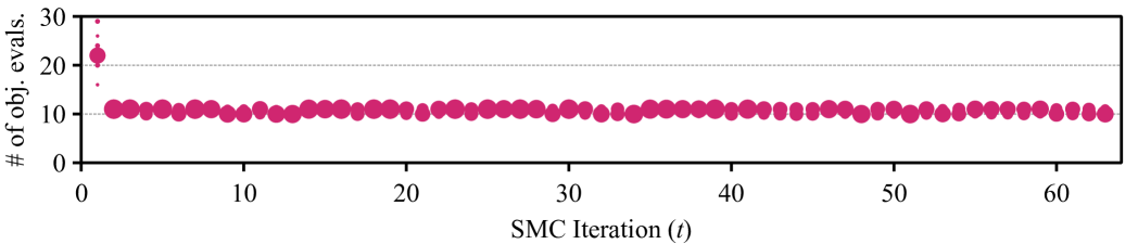
(b)

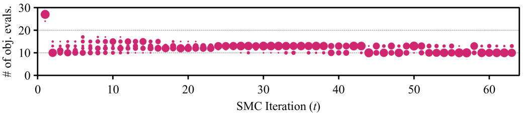
(c)

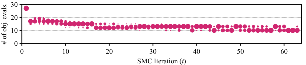
(d)

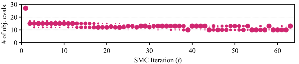
(e)

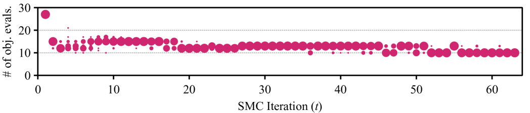
(f)

Figure 20: Number of objective evaluations spent during adaptation at each SMC iteration (continued). The size of the markers represents the proportion of runs that spent each respective number of evaluations among 32 independent runs.

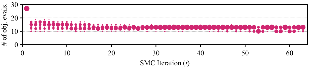
(a)

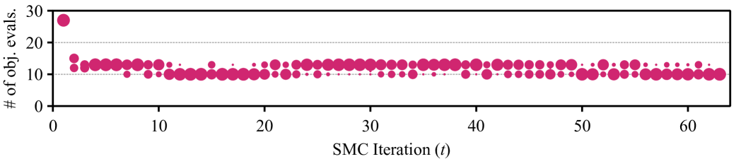
(b)

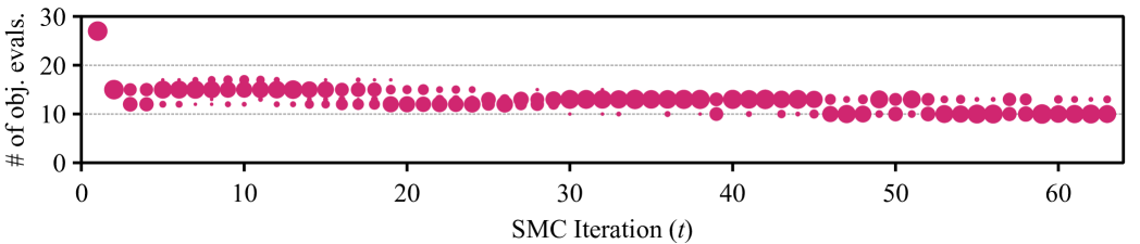
(c)

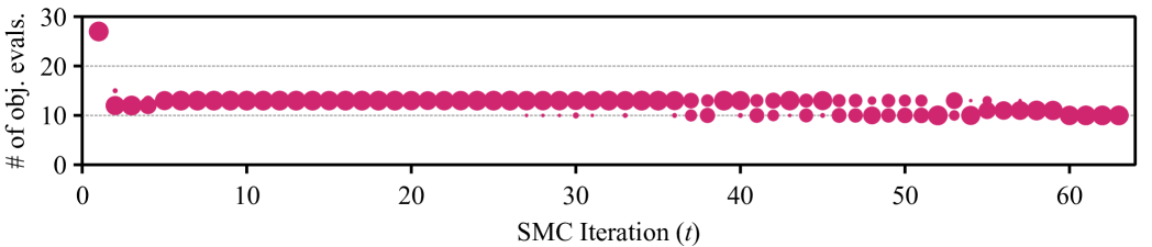
(d)

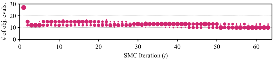
(e)

Figure 21: Number of objective evaluations spent during adaptation at each SMC iteration (continued). The size of the markers represents the proportion of runs that spent each respective number of evaluations among 32 independent runs.

F.3.2 SMC-KLMC

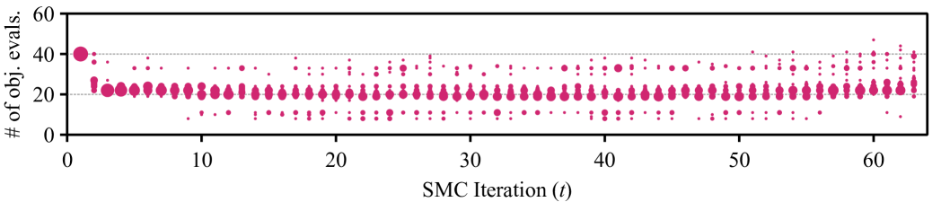
(a)

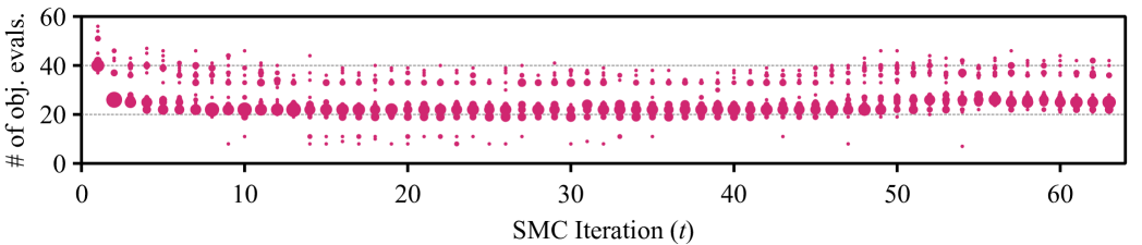
(b)

(c)

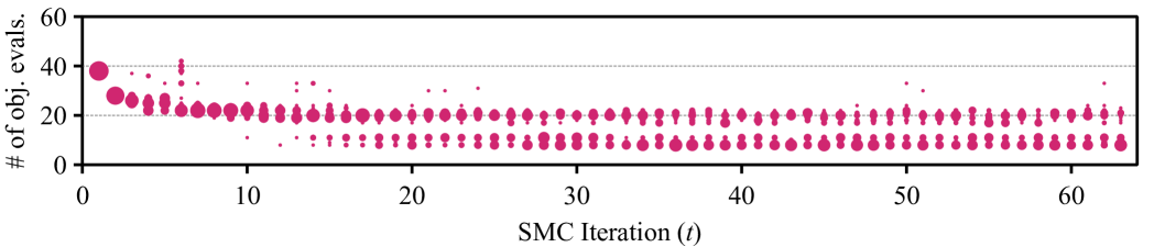
(d)

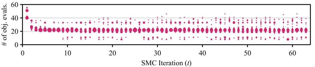
(e)

Figure 22: Number of objective evaluations spent during adaptation at each SMC iteration. The size of the markers represents the proportion of runs that spent each respective number of evaluations among 32 independent runs.

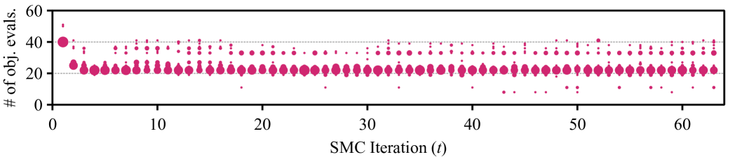
(a)

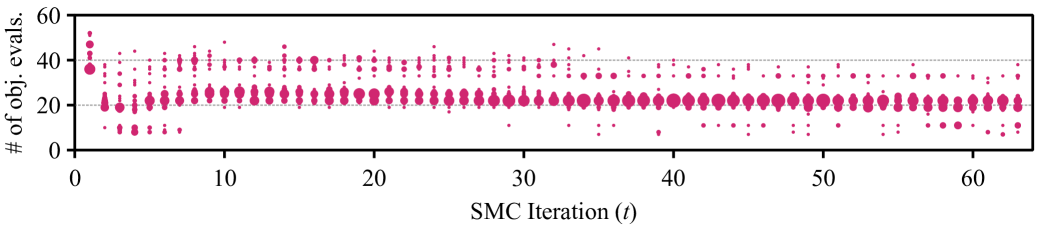
(b)

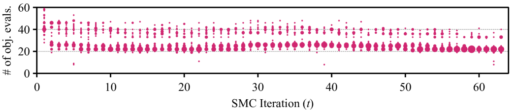
(c)

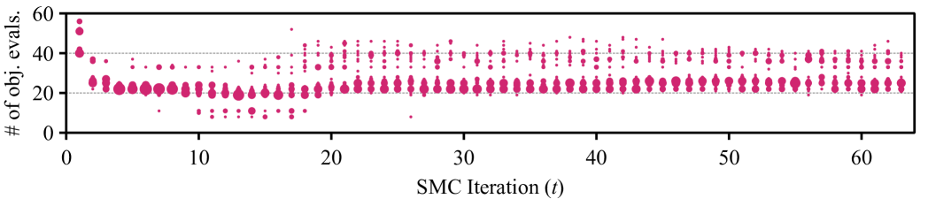
(d)

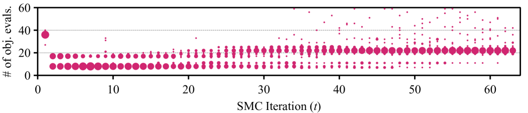
(e)

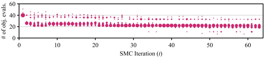
(f)

Figure 23: Number of objective evaluations spent during adaptation at each SMC iteration (continued). The size of the markers represents the proportion of runs that spent each respective number of evaluations among 32 independent runs.

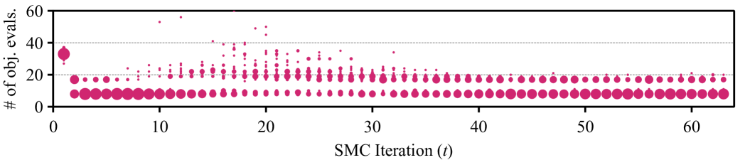
(a)

(b)

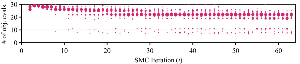
(c)

(d)

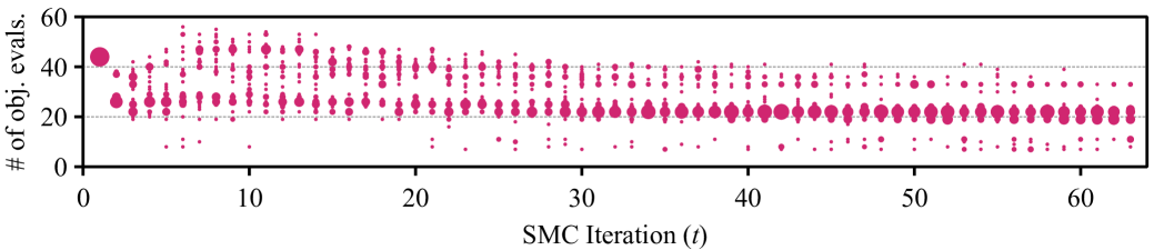
(e)

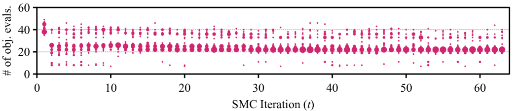
(f)

Figure 24: Number of objective evaluations spent during adaptation at each SMC iteration (continued). The size of the markers represents the proportion of runs that spent each respective number of evaluations among 32 independent runs.

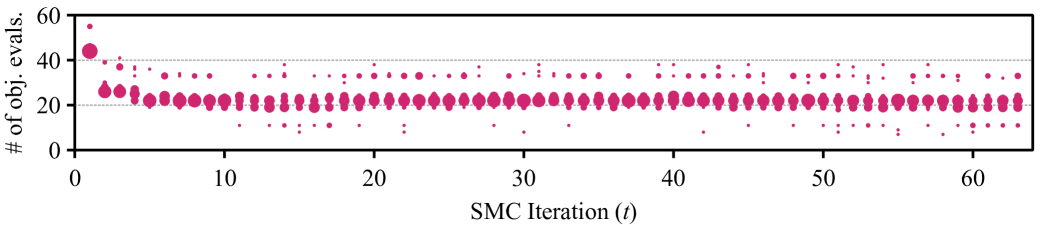
(a)

(b)

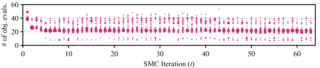
(c)

(d)

Figure 25: Number of objective evaluations spent during adaptation at each SMC iteration (continued). The size of the markers represents the proportion of runs that spent each respective number of evaluations among 32 independent runs.

F.4 Adaptation Results from the Adaptive SMC Samplers

Finally, we will present additional results generated from our adaptive SMC samplers, including the adapted temperature schedule, stepsize schedule, and normalizing constant estimates. The computational budgets are set as $T_{1}=64$ and $N=1024$ with $B=256$.

F.4.1 SMC-LMC

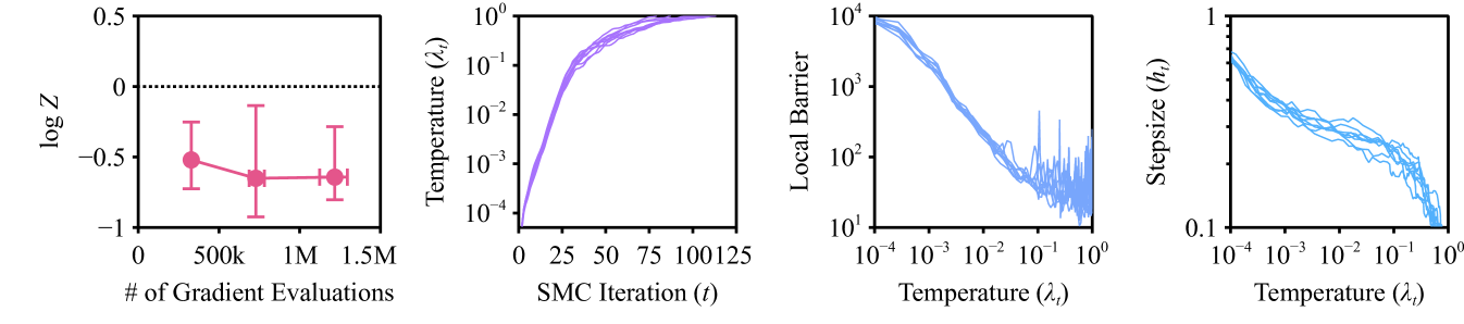
(a)

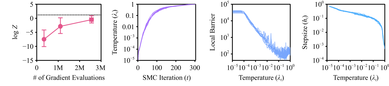
(b)

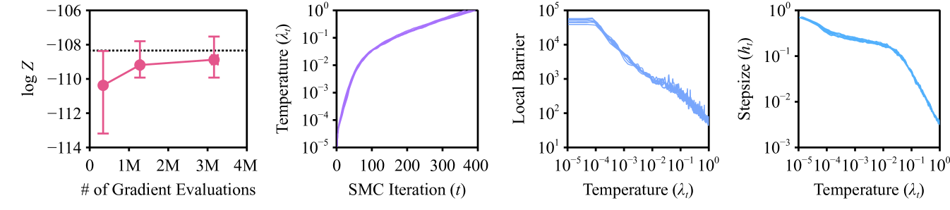
(c)

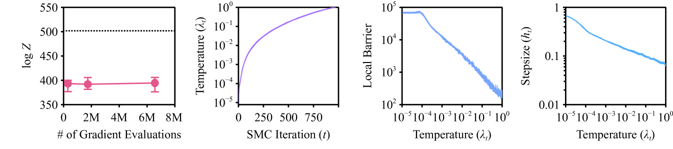
(d)

Figure 26: Normalizing constant estimate, temperature schedule, local communication barrier, and stepsize schedules obtained by running SMC-LMC. The dotted line is the ground truth value obtained from a large budget run. For the normalizing constant estimate, the confidence intervals in the vertical and horizontal directions are the $80\%$ quantiles obtained from 32 replications. The temperature schedule, local communication barriers, and the step sizes from a subset of 8 runs are shown.

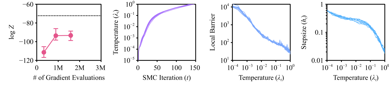
(a)

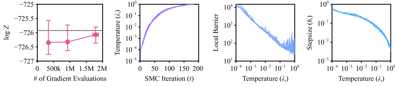
(b)

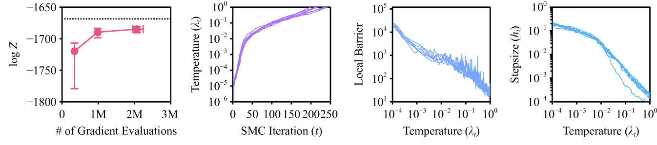
(c)

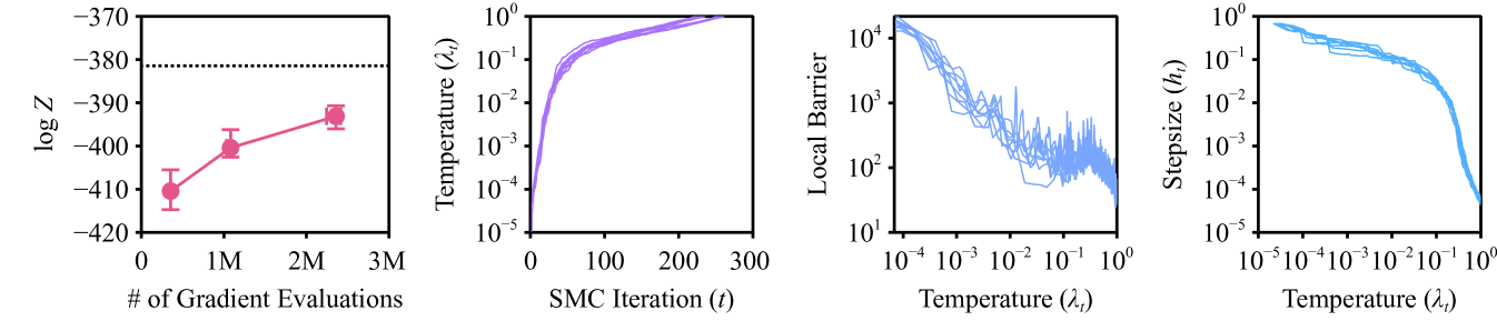
(d)

Figure 27: Normalizing constant estimate, temperature schedule, local communication barrier, and stepsize schedules obtained by running SMC-LMC (continued). The dotted line is the ground truth value obtained from a large budget run. For the normalizing constant estimate, the confidence intervals in the vertical and horizontal directions are the $80\%$ quantiles obtained from 32 replications. The temperature schedule, local communication barriers, and the step sizes from a subset of 8 runs are shown.

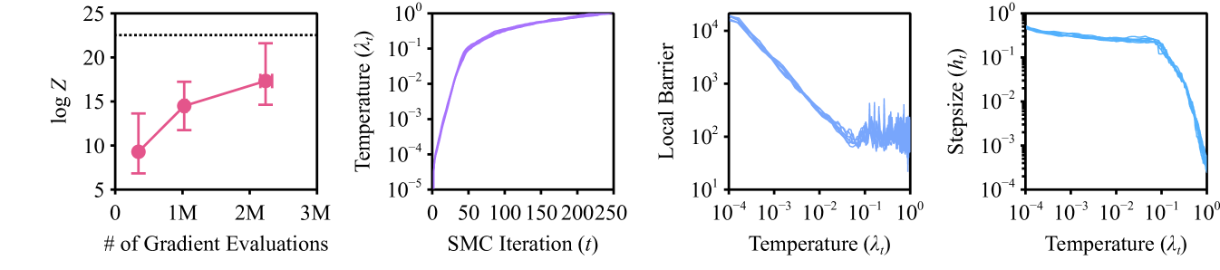
(a)

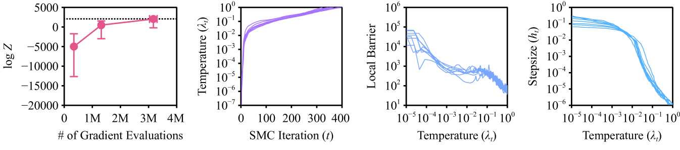
(b)

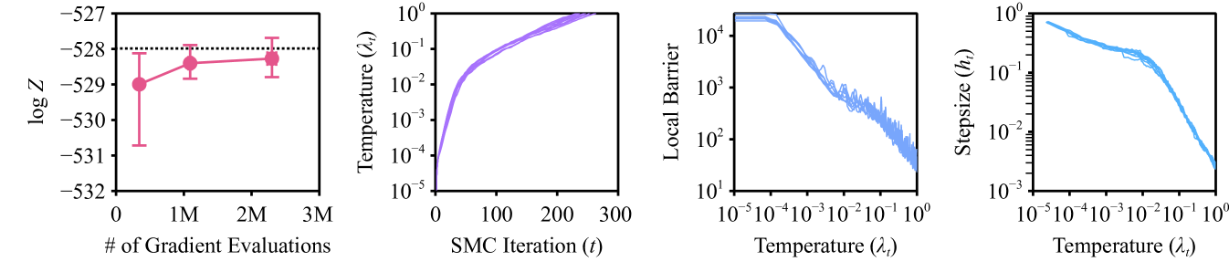
(c)

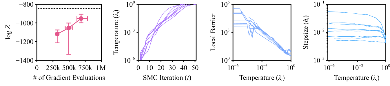
(d)

Figure 28: Normalizing constant estimate, temperature schedule, local communication barrier, and stepsize schedules obtained by running SMC-LMC (continued). The dotted line is the ground truth value obtained from a large budget run. For the normalizing constant estimate, the confidence intervals in the vertical and horizontal directions are the $80\%$ quantiles obtained from 32 replications. The temperature schedule, local communication barriers, and the step sizes from a subset of 8 runs are shown.

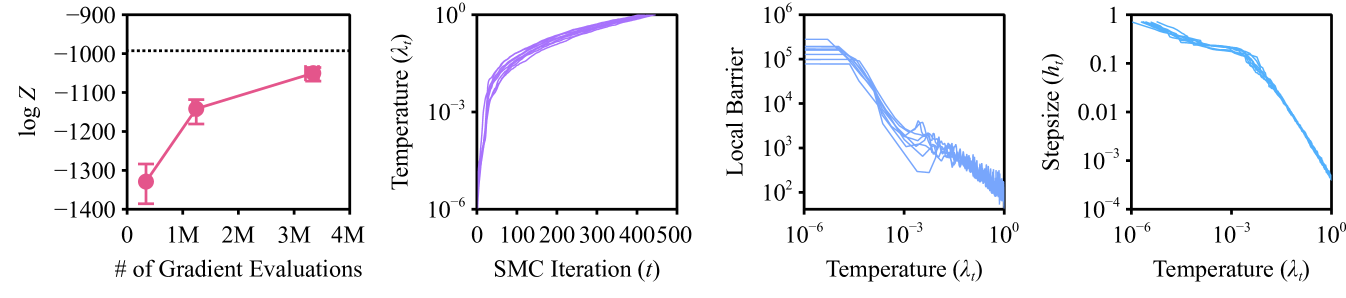
(a)

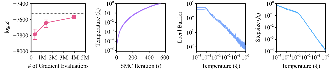
(b)

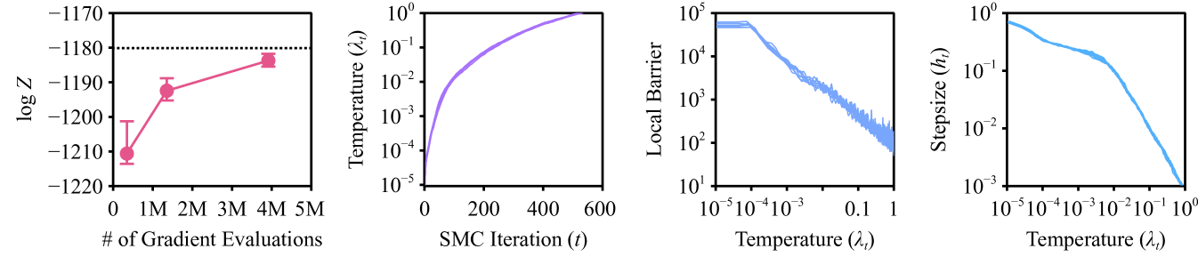
(c)

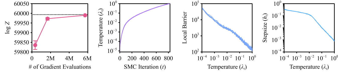
(d)

Figure 29: Normalizing constant estimate, temperature schedule, local communication barrier, and stepsize schedules obtained by running SMC-LMC (continued). The dotted line is the ground truth value obtained from a large budget run. For the normalizing constant estimate, the confidence intervals in the vertical and horizontal directions are the $80\%$ quantiles obtained from 32 replications. The temperature schedule, local communication barriers, and the step sizes from a subset of 8 runs are shown.

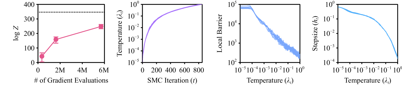
(a)

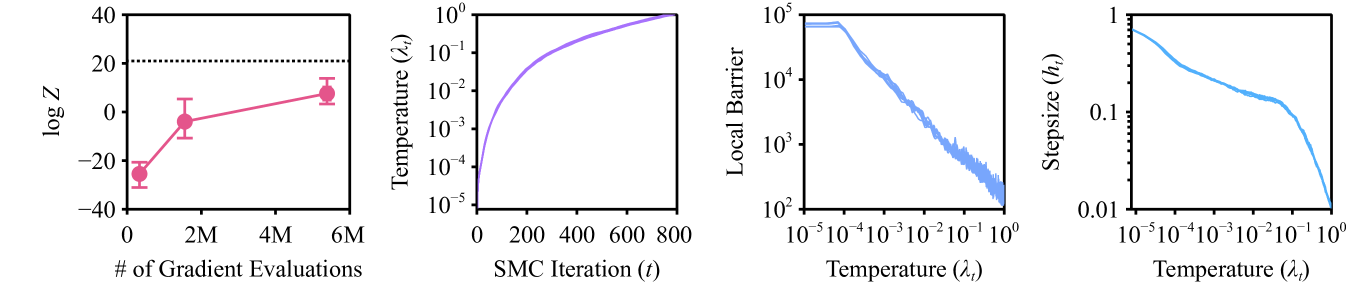
(b)

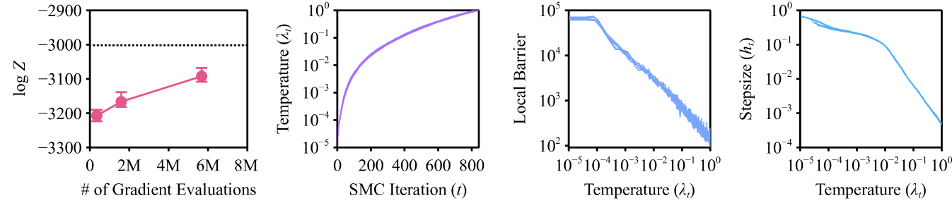
(c)

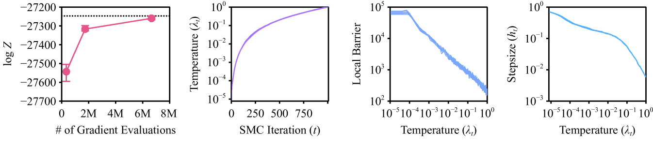
(d)

Figure 30: Normalizing constant estimate, temperature schedule, local communication barrier, and stepsize schedules obtained by running SMC-LMC (continued). The dotted line is the ground truth value obtained from a large budget run. For the normalizing constant estimate, the confidence intervals in the vertical and horizontal directions are the $80\%$ quantiles obtained from 32 replications. The temperature schedule, local communication barriers, and the step sizes from a subset of 8 runs are shown.

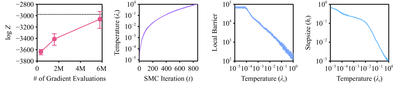
(a)

Figure 31: Normalizing constant estimate, temperature schedule, local communication barrier, and stepsize schedules obtained by running SMC-LMC (continued). The dotted line is the ground truth value obtained from a large budget run. For the normalizing constant estimate, the confidence intervals in the vertical and horizontal directions are the $80\%$ quantiles obtained from 32 replications. The temperature schedule, local communication barriers, and the step sizes from a subset of 8 runs are shown.

F.4.2 SMC-KLMC

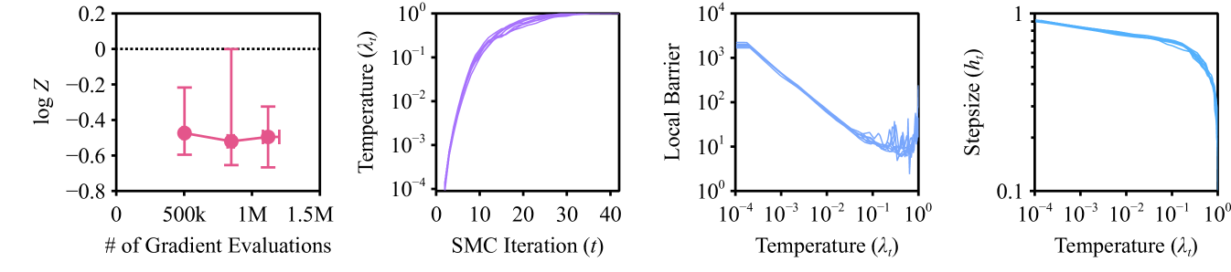
(a)

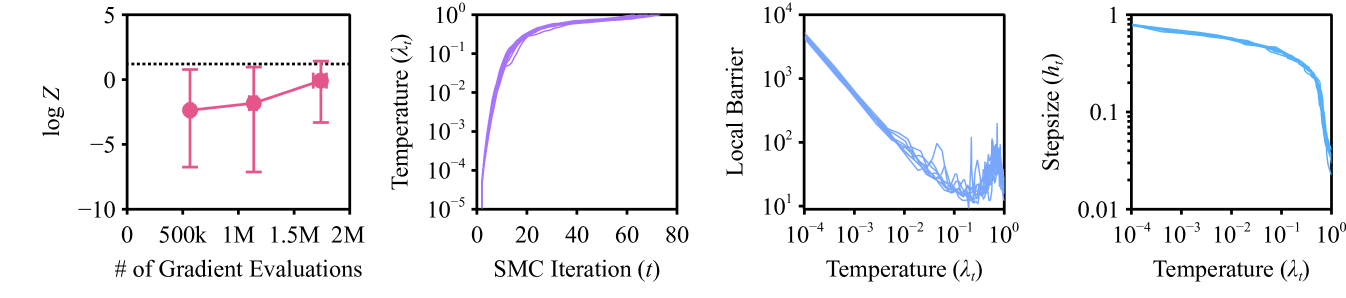
(b)

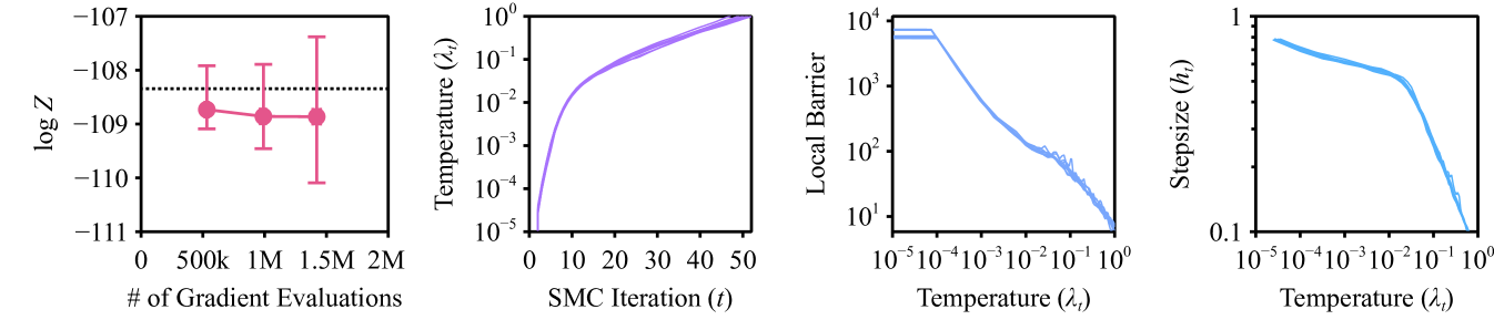
(c)

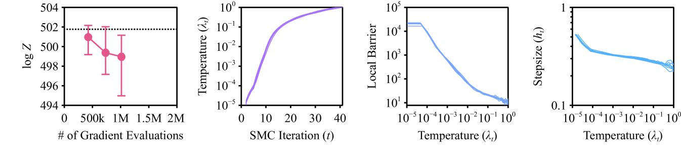
(d)

Figure 32: Normalizing constant estimate, temperature schedule, local communication barrier, and stepsize schedules obtained by running SMC-KLMC. The dotted line is the ground truth value obtained from a large budget run. For the normalizing constant estimate, the confidence intervals in the vertical and horizontal directions are the $80\%$ quantiles obtained from 32 replications. The temperature schedule, local communication barriers, and the step sizes from a subset of 8 runs are shown.

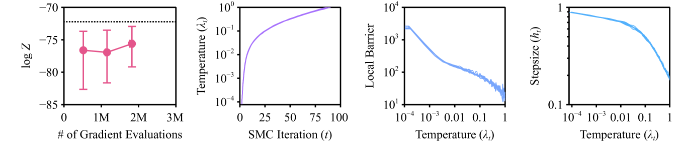
(a)

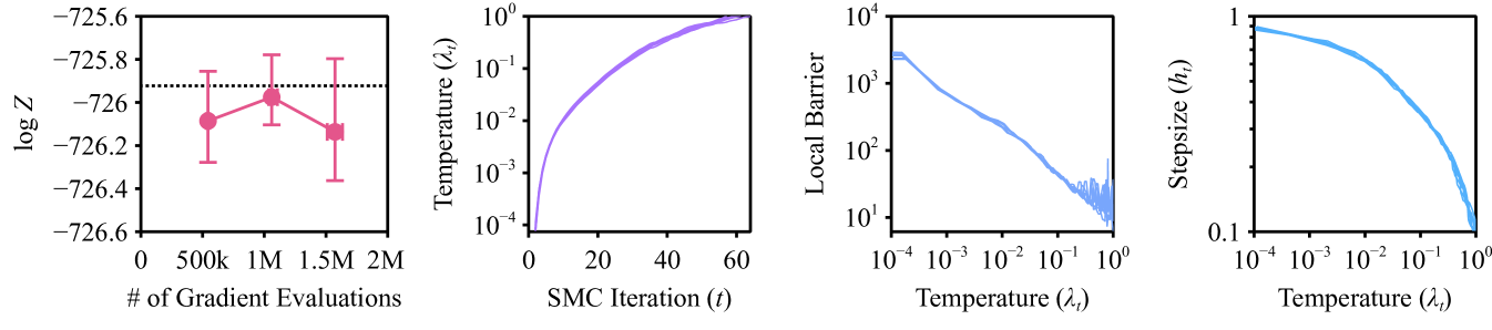
(b)

(c)

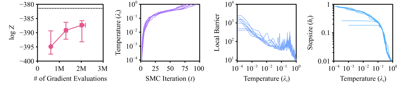
(d)

Figure 33: Normalizing constant estimate, temperature schedule, local communication barrier, and stepsize schedules obtained by running SMC-KLMC (continued). The dotted line is the ground truth value obtained from a large budget run. For the normalizing constant estimate, the confidence intervals in the vertical and horizontal directions are the $80\%$ quantiles obtained from 32 replications. The temperature schedule, local communication barriers, and the step sizes from a subset of 8 runs are shown.

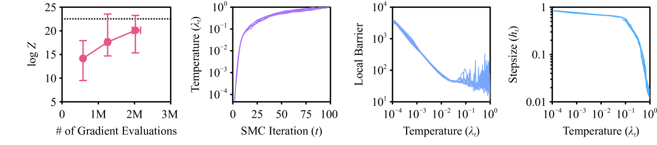
(a)

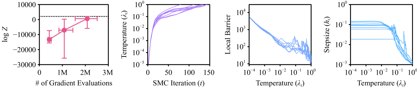
(b)

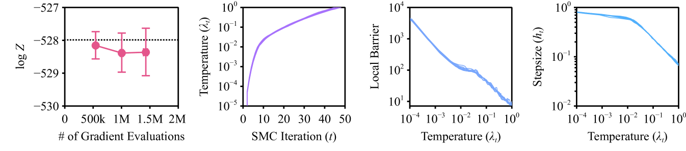
(c)

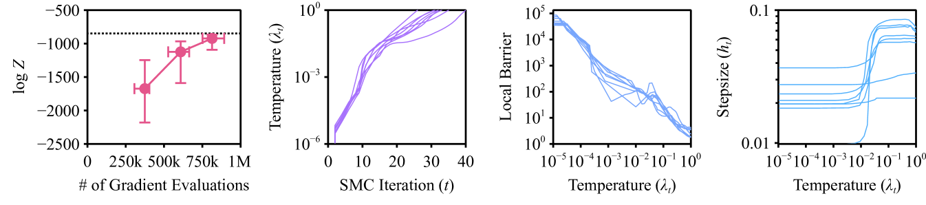
(d)

Figure 34: Normalizing constant estimate, temperature schedule, local communication barrier, and stepsize schedules obtained by running SMC-KLMC (continued). The dotted line is the ground truth value obtained from a large budget run. For the normalizing constant estimate, the confidence intervals in the vertical and horizontal directions are the $80\%$ quantiles obtained from 32 replications. The temperature schedule, local communication barriers, and the step sizes from a subset of 8 runs are shown.

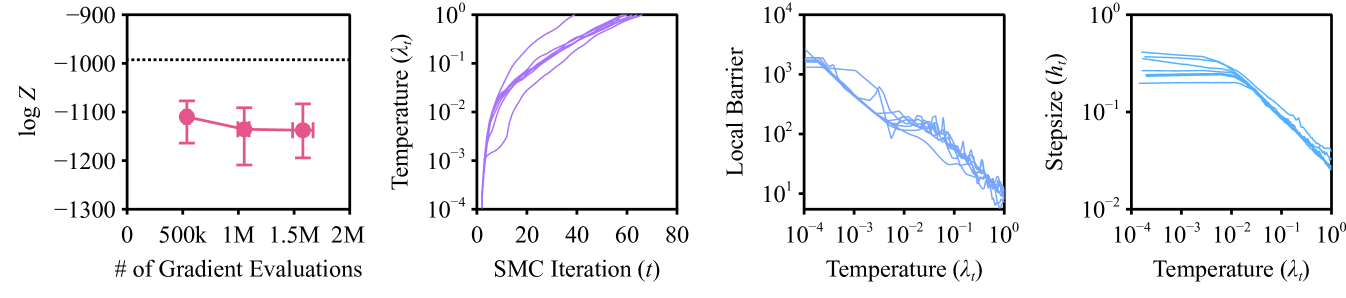
(a)

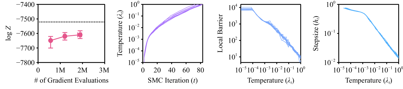
(b)

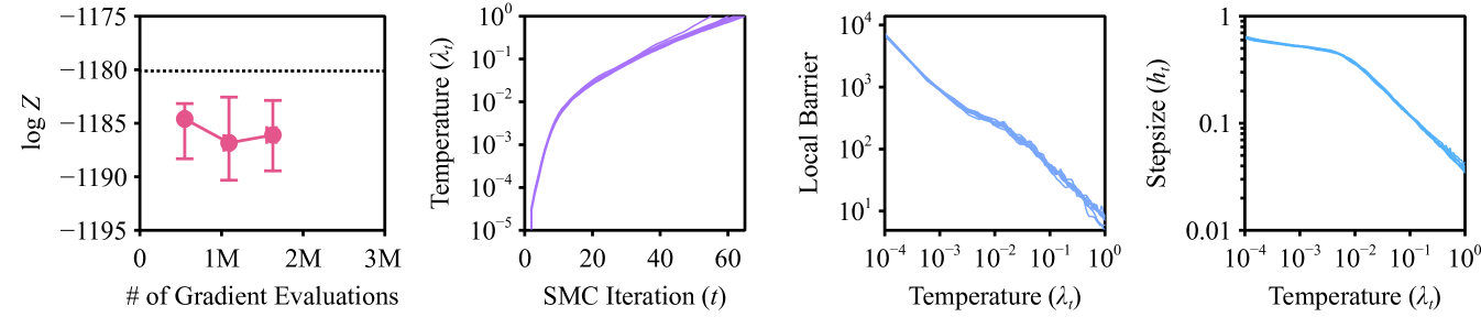
(c)

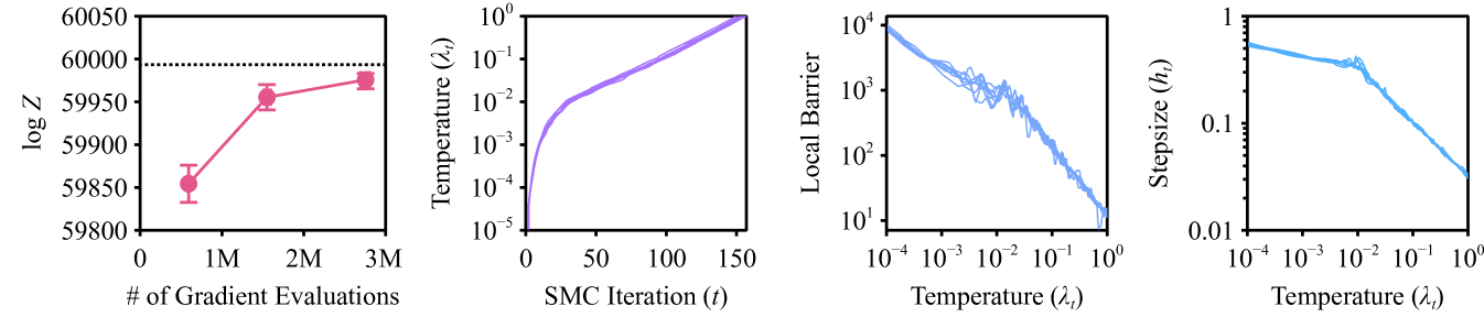
(d)

Figure 35: Normalizing constant estimate, temperature schedule, local communication barrier, and stepsize schedules obtained by running SMC-KLMC (continued). The dotted line is the ground truth value obtained from a large budget run. For the normalizing constant estimate, the confidence intervals in the vertical and horizontal directions are the $80\%$ quantiles obtained from 32 replications. The temperature schedule, local communication barriers, and the step sizes from a subset of 8 runs are shown.

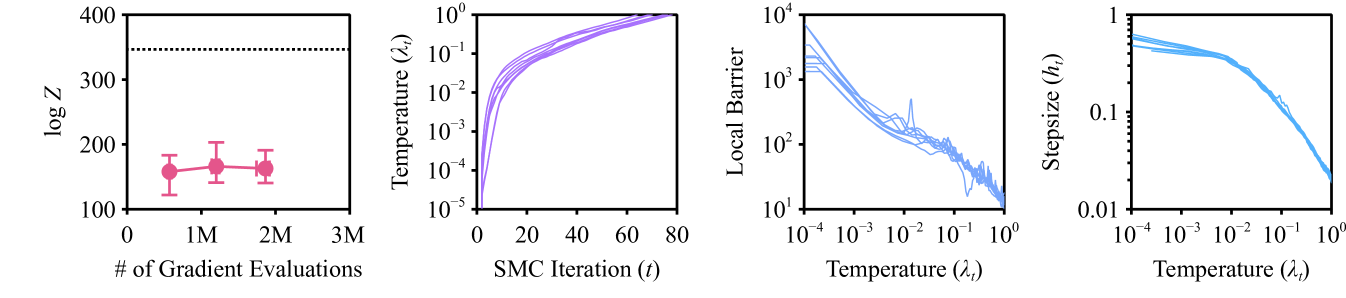
(a)

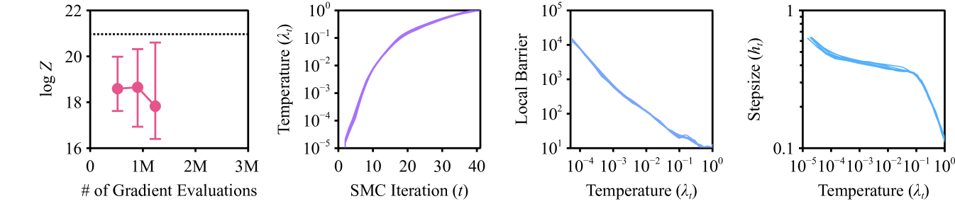
(b)

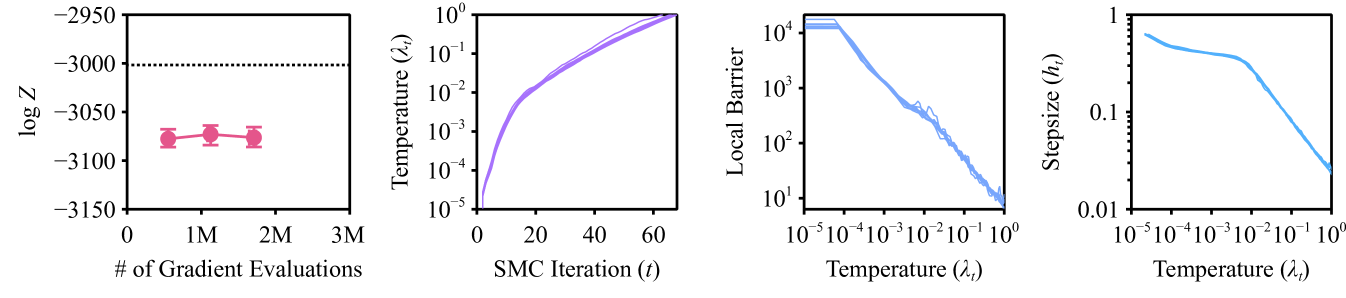
(c)

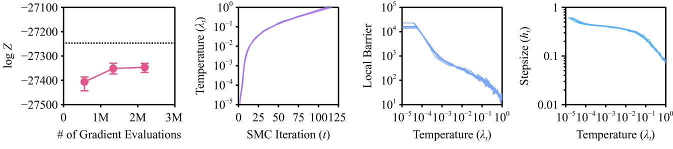
(d)

Figure 36: Normalizing constant estimate, temperature schedule, local communication barrier, and stepsize schedules obtained by running SMC-KLMC (continued). The dotted line is the ground truth value obtained from a large budget run. For the normalizing constant estimate, the confidence intervals in the vertical and horizontal directions are the $80\%$ quantiles obtained from 32 replications. The temperature schedule, local communication barriers, and the step sizes from a subset of 8 runs are shown.

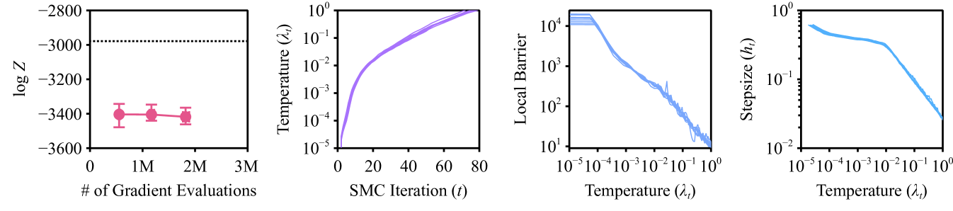
(a)

Figure 37: Normalizing constant estimate, temperature schedule, local communication barrier, and stepsize schedules obtained by running SMC-KLMC (continued). The dotted line is the ground truth value obtained from a large budget run. For the normalizing constant estimate, the confidence intervals in the vertical and horizontal directions are the $80\%$ quantiles obtained from 32 replications. The temperature schedule, local communication barriers, and the step sizes from a subset of 8 runs are shown.

References

- Achituve et al. (2025) Achituve, I., Habi, H. V., Rosenfeld, A., Netzer, A., Diamant, I., and Fetaya, E. Inverse problem sampling in latent space using sequential Monte Carlo. ArXiv Preprint arXiv:2502.05908, arXiv, 2025.
- Andrieu & Robert (2001) Andrieu, C. and Robert, C. P. Controlled MCMC for optimal sampling. Technical Report 0125, Université Paris-Dauphine, 2001.
- Arbel et al. (2021) Arbel, M., Matthews, A., and Doucet, A. Annealed flow transport Monte Carlo. In Proceedings of the International Conference on Machine Learning, volume 139 of PMLR, pp. 318–330. JMLR, 2021.
- Atchadé & Rosenthal (2005) Atchadé, Y. F. and Rosenthal, J. S. On adaptive Markov chain Monte Carlo algorithms. Bernoulli, 11(5), 2005.
- Avriel & Wilde (1968) Avriel, M. and Wilde, D. J. Golden block search for the maximum of unimodal functions. Management Science, 14(5):307–319, 1968.
- Bentley & Yao (1976) Bentley, J. L. and Yao, A. C.-C. An almost optimal algorithm for unbounded searching. Information Processing Letters, 5(3):82–87, 1976.
- Bernton et al. (2019) Bernton, E., Heng, J., Doucet, A., and Jacob, P. E. Schrödinger bridge samplers. ArXiv Preprint arXiv:1912.13170, arXiv, 2019.
- Besag (1994) Besag, J. E. Comments on ‘Representations of knowledge in complex systems’ by U. Grenander and M.I. Miller. Journal of the Royal Statistical Society Series B (Statistical Methodology), 56(4):591–592, 1994.
- Beskos et al. (2016) Beskos, A., Jasra, A., Kantas, N., and Thiery, A. On the convergence of adaptive sequential Monte Carlo methods. The Annals of Applied Probability, 26(2):1111–1146, 2016.
- Bezanson et al. (2017) Bezanson, J., Edelman, A., Karpinski, S., and Shah, V. B. Julia: A fresh approach to numerical computing. SIAM Review, 59(1):65–98, 2017.
- Biswas et al. (2019) Biswas, N., Jacob, P. E., and Vanetti, P. Estimating convergence of Markov chains with L-lag couplings. In Advances in Neural Information Processing Systems, volume 32, pp. 7391–7401. Curran Associates, Inc., 2019.
- Blei et al. (2003) Blei, D. M., Ng, A. Y., and Jordan, M. I. Latent Dirichlet allocation. Journal of Machine Learning Research, 3(null):993–1022, 2003.
- Bottou et al. (2018) Bottou, L., Curtis, F. E., and Nocedal, J. Optimization methods for large-scale machine learning. SIAM Review, 60(2):223–311, 2018.
- Bradbury et al. (2018) Bradbury, J., Frostig, R., Hawkins, P., Johnson, M. J., Leary, C., Maclaurin, D., Necula, G., Paszke, A., VanderPlas, J., Wanderman-Milne, S., and Zhang, Q. JAX: Composable transformations of Python+NumPy programs, 2018.
- Buchholz et al. (2021) Buchholz, A., Chopin, N., and Jacob, P. E. Adaptive tuning of Hamiltonian Monte Carlo within sequential Monte Carlo. Bayesian Analysis, 16(3):745–771, 2021.
- Cappé et al. (2005) Cappé, O., Rydén, T., and Moulines, E. Inference in Hidden Markov Models. Springer Series in Statistics. Springer, Berlin [u.a.], online-ausg. edition, 2005.
- Cappé et al. (2007) Cappé, O., Godsill, S. J., and Moulines, E. An overview of existing methods and recent advances in sequential Monte Carlo. Proceedings of the IEEE, 95(5):899–924, 2007.
- Cardoso et al. (2024) Cardoso, G., Janati el idrissi, Y., Le Corff, S., and Moulines, E. Monte Carlo guided denoising diffusion models for Bayesian linear inverse problems. In Proceedings of the International Conference on Learning Representations, 2024.
- Carpenter et al. (1999) Carpenter, J., Clifford, P., and Fearnhead, P. Improved particle filter for nonlinear problems. IEE Proceedings - Radar, Sonar and Navigation, 146(1):2, 1999.
- Caterini et al. (2018) Caterini, A. L., Doucet, A., and Sejdinovic, D. Hamiltonian variational auto-encoder. In Advances in Neural Information Processing Systems, volume 31, pp. 8167–8177. Curran Associates, Inc., 2018.
- Chehab et al. (2023) Chehab, O., Hyvarinen, A., and Risteski, A. Provable benefits of annealing for estimating normalizing constants: Importance sampling, noise-contrastive estimation, and beyond. In Advances in Neural Information Processing Systems, volume 36, pp. 45945–45970, 2023.
- Chewi et al. (2021) Chewi, S., Lu, C., Ahn, K., Cheng, X., Gouic, T. L., and Rigollet, P. Optimal dimension dependence of the Metropolis-adjusted Langevin algorithm. In Proceedings of the Conference on Learning Theory, volume 134 of PMLR, pp. 1260–1300. JMLR, 2021.
- Chopin (2002) Chopin, N. A sequential particle filter method for static models. Biometrika, 89(3):539–552, 2002.
- Chopin (2004) Chopin, N. Central limit theorem for sequential Monte Carlo methods and its application to Bayesian inference. The Annals of Statistics, 32(6), 2004.
- Chopin & Papaspiliopoulos (2020) Chopin, N. and Papaspiliopoulos, O. An Introduction to Sequential Monte Carlo. Springer Series in Statistics. Springer International Publishing, Cham, 2020.
- Commandeur & Koopman (2007) Commandeur, J. J. F. and Koopman, S. J. An Introduction to State Space Time Series Analysis. Practical Econometrics Series. Oxford University Press, Oxford, 2007.
- Cooney (2017) Cooney, M. Modelling loss curves in insurance with RStan. Stan Case Study, 2017.
- Crowder (1978) Crowder, M. J. Beta-binomial ANOVA for proportions. Journal of the Royal Statistical Society: Series C (Applied Statistics), 27(1):34–37, 1978.
- Dai et al. (2022) Dai, C., Heng, J., Jacob, P. E., and Whiteley, N. An invitation to sequential Monte Carlo samplers. Journal of the American Statistical Association, 117(539):1587–1600, 2022.
- Dalalyan (2017) Dalalyan, A. S. Theoretical guarantees for approximate sampling from smooth and log-concave densities. Journal of the Royal Statistical Society Series B: Statistical Methodology, 79(3):651–676, 2017.
- Dau & Chopin (2022) Dau, H.-D. and Chopin, N. Waste-free sequential Monte Carlo. Journal of the Royal Statistical Society Series B: Statistical Methodology, 84(1):114–148, 2022.
- Del Moral (2004) Del Moral, P. Feynman-Kac Formulae: Genealogical and Interacting Particle Systems with Applications. Probability and Its Applications. Springer, New York, New York, 2004.
- Del Moral (2016) Del Moral, P. Mean Field Simulation for Monte Carlo Integration. Chapman & Hall/CRC, Boca Raton, 2016.
- Del Moral et al. (2006) Del Moral, P., Doucet, A., and Jasra, A. Sequential Monte Carlo samplers. Journal of the Royal Statistical Society Series B (Statistical Methodology), 68(3):411–436, 2006.
- Dorazio et al. (2006) Dorazio, R. M., Royle, J. A., Söderström, B., and Glimskär, A. Estimating species richness and accumulation by modeling species occurrence and detectability. Ecology, 87(4):842–854, 2006.
- Dou & Song (2024) Dou, Z. and Song, Y. Diffusion posterior sampling for linear inverse problem solving: A filtering perspective. In Proceedings of the International Conference on Learning Representations, 2024.
- Doucet & Johansen (2011) Doucet, A. and Johansen, A. M. A tutorial on particle filtering and smoothing: Fifteen years later. In Oxford Handbook of Nonlinear Filtering, Oxford Handbooks. Oxford University Press, 2011.
- Doucet et al. (2022) Doucet, A., Grathwohl, W., Matthews, A. G., and Strathmann, H. Score-based diffusion meets annealed importance sampling. In Advances in Neural Information Processing Systems, volume 35, pp. 21482–21494, 2022.
- Doucet et al. (2023) Doucet, A., Moulines, E., and Thin, A. Differentiable samplers for deep latent variable models. Philosophical Transactions of the Royal Society A: Mathematical, Physical and Engineering Sciences, 381(2247):20220147, 2023.
- Duane et al. (1987) Duane, S., Kennedy, A. D., Pendleton, B. J., and Roweth, D. Hybrid Monte Carlo. Physics Letters B, 195(2):216–222, 1987.
- Durmus & Eberle (2024) Durmus, A. and Eberle, A. Asymptotic bias of inexact Markov chain Monte Carlo methods in high dimension. The Annals of Applied Probability, 34(4):3435–3468, 2024.
- Durmus & Moulines (2019) Durmus, A. and Moulines, É. High-dimensional Bayesian inference via the unadjusted Langevin algorithm. Bernoulli, 25(4A), 2019.
- Elvira et al. (2022) Elvira, V., Martino, L., and Robert, C. P. Rethinking the effective sample size. International Statistical Review, pp. insr.12500, 2022.
- Farkas (2014) Farkas, A. Three men and a boat, translated by andras farkas to french and swedish, 2014.
- Fearnhead & Taylor (2013) Fearnhead, P. and Taylor, B. M. An adaptive sequential Monte Carlo sampler. Bayesian Analysis, 8(2):411–438, 2013.
- Furr (2017) Furr, D. C. Rating scale and generalized rating scale models with latent regression. Stan Case Study, 2017.
- Geffner & Domke (2021) Geffner, T. and Domke, J. MCMC variational inference via uncorrected Hamiltonian annealing. In Advances in Neural Information Processing Systems, volume 34, pp. 639–651. Curran Associates, Inc., 2021.
- Geffner & Domke (2023) Geffner, T. and Domke, J. Langevin diffusion variational inference. In Proceedings of the International Conference on Artificial Intelligence and Statistics, volume 206 of PMLR, pp. 576–593. JMLR, 2023.
- Gelfand et al. (1990) Gelfand, A. E., Hills, S. E., Racine-Poon, A., and Smith, A. F. M. Illustration of Bayesian inference in normal data models using Gibbs sampling. Journal of the American Statistical Association, 85(412):972–985, 1990.
- Gelman & Hill (2007) Gelman, A. and Hill, J. Data Analysis Using Regression and Multilevel/Hierarchical Models. Analytical Methods for Social Research. Cambridge University Press, 2007.
- Gelman et al. (2014) Gelman, A., Carlin, J., Stern, H., Dunson, D., Vehtari, A., and Rubin, D. Bayesian Data Analysis. Chapman & Hall/CRC Texts in Statistical Science. CRC Press, Boca Raton, 3 edition, 2014.
- Geman & Geman (1984) Geman, S. and Geman, D. Stochastic relaxation, Gibbs distributions, and the Bayesian restoration of images. IEEE Transactions on Pattern Analysis and Machine Intelligence, 6(6):721–741, 1984.
- Gerber et al. (2019) Gerber, M., Chopin, N., and Whiteley, N. Negative association, ordering and convergence of resampling methods. The Annals of Statistics, 47(4):2236–2260, 2019.
- Gorman & Sejnowski (1988) Gorman, R. and Sejnowski, T. J. Analysis of hidden units in a layered network trained to classify sonar targets. Neural Networks, 1(1):75–89, 1988.
- Goshtasbpour & Perez-Cruz (2023) Goshtasbpour, S. and Perez-Cruz, F. Optimization of annealed importance sampling hyperparameters. In Machine Learning and Knowledge Discovery in Databases, volume 13717 of LNCS, pp. 174–190, Cham, 2023. Springer Nature Switzerland.
- Goshtasbpour et al. (2023) Goshtasbpour, S., Cohen, V., and Perez-Cruz, F. Adaptive annealed importance sampling with constant rate progress. In Proceedings of the International Conference on Machine Learning, pp. 11642–11658. PMLR, 2023.
- Grenander & Miller (1994) Grenander, U. and Miller, M. I. Representations of knowledge in complex systems. Journal of the Royal Statistical Society: Series B (Methodological), 56(4):549–581, 1994.
- Gu et al. (2015) Gu, S. S., Ghahramani, Z., and Turner, R. E. Neural adaptive sequential Monte Carlo. In Advances in Neural Information Processing Systems, volume 28, pp. 2629–2637. Curran Associates, Inc., 2015.
- Hastings (1970) Hastings, W. K. Monte Carlo sampling methods using Markov chains and their applications. Biometrika, 57(1):97–109, 1970.
- Heng et al. (2020) Heng, J., Bishop, A. N., Deligiannidis, G., and Doucet, A. Controlled sequential Monte Carlo. The Annals of Statistics, 48(5):2904–2929, 2020.
- Horowitz (1991) Horowitz, A. M. A generalized guided Monte Carlo algorithm. Physics Letters B, 268(2):247–252, 1991.
- Jasra et al. (2011) Jasra, A., Stephens, D. A., Doucet, A., and Tsagaris, T. Inference for Lévy-driven stochastic volatility models via adaptive sequential Monte Carlo. Scandinavian Journal of Statistics, 38(1):1–22, 2011.
- Kéry & Schaub (2012) Kéry, M. M. M. and Schaub, M. Bayesian Population Analysis Using WinBUGS: A Hierarchical Perspective. Academic Press, Waltham, MA, 1 edition, 2012.
- Kiefer (1953) Kiefer, J. Sequential minimax search for a maximum. Proceedings of the American Mathematical Society, 4(3):502–506, 1953.
- Kim et al. (2015) Kim, S., Pasupathy, R., and Henderson, S. G. A guide to sample average approximation. In Handbook of Simulation Optimization, pp. 207–243. Springer, New York, NY, 2015.
- Kingma & Ba (2015) Kingma, D. P. and Ba, J. Adam: A method for stochastic optimization. In Proceedings of the International Conference on Learning Representations, San Diego, California, USA, 2015.
- Kitagawa (1996) Kitagawa, G. Monte Carlo filter and smoother for non-gaussian nonlinear state space models. Journal of Computational and Graphical Statistics, 5(1):1–25, 1996.
- Kiwaki (2015) Kiwaki, T. Variational optimization of annealing schedules. ArXiv Preprint arXiv:1502.05313, arXiv, 2015.
- Kong (1992) Kong, A. A note on importance sampling using standardized weights. Technical Report 348, Department of Statistics, University of Chicago, 1992.
- Kullback & Leibler (1951) Kullback, S. and Leibler, R. A. On information and sufficiency. The Annals of Mathematical Statistics, 22(1):79–86, 1951.
- Lavrov (2017) Lavrov, M. Answer to “Golden section search initial values”, 2017.
- Le et al. (2018) Le, T. A., Igl, M., Rainforth, T., Jin, T., and Wood, F. Auto-encoding sequential Monte Carlo. In Proceedings of the International Conference on Learning Representations, 2018.
- Lee et al. (2021) Lee, Y. T., Shen, R., and Tian, K. Lower bounds on Metropolized sampling methods for well-conditioned distributions. In Advances in Neural Information Processing Systems, volume 34, pp. 18812–18824. Curran Associates, Inc., 2021.
- Leimkuhler & Matthews (2013) Leimkuhler, B. and Matthews, C. Rational construction of stochastic numerical methods for molecular sampling. Applied Mathematics Research eXpress, 2013(1):34–56, 2013.
- Lew et al. (2023) Lew, A. K., Zhi-Xuan, T., Grand, G., and Mansinghka, V. Sequential Monte Carlo steering of large language models using probabilistic programs. In ICML Workshop: Sampling and Optimization in Discrete Space, 2023.
- Luenberger & Ye (2008) Luenberger, D. G. and Ye, Y. Linear and Nonlinear Programming, volume 116 of International Series in Operations Research & Management Science. Springer US, New York, NY, 2008.
- Ma et al. (2021) Ma, Y.-A., Chatterji, N. S., Cheng, X., Flammarion, N., Bartlett, P. L., and Jordan, M. I. Is there an analog of Nesterov acceleration for gradient-based MCMC? Bernoulli, 27(3):1942–1992, 2021.
- Maddison et al. (2017) Maddison, C. J., Lawson, J., Tucker, G., Heess, N., Norouzi, M., Mnih, A., Doucet, A., and Teh, Y. Filtering variational objectives. In Advances in Neural Information Processing Systems, volume 30, pp. 6573–6583. Curran Associates, Inc., 2017.
- Magnusson et al. (2022) Magnusson, M., Bürkner, P., and Vehtari, A. Posteriordb: A set of posteriors for Bayesian inference and probabilistic programming, 2022.
- Magnusson et al. (2025) Magnusson, M., Torgander, J., Bürkner, P.-C., Zhang, L., Carpenter, B., and Vehtari, A. posteriordb: Testing, benchmarking and developing Bayesian inference algorithms. In Proceedings of the International Conference on Artificial Intelligence and Statistics (to Appear), 2025.
- Masrani et al. (2021) Masrani, V., Brekelmans, R., Bui, T., Nielsen, F., Galstyan, A., Steeg, G. V., and Wood, F. Q-Paths: Generalizing the geometric annealing path using power means. In Proceedings of the Conference on Uncertainty in Artificial Intelligence, volume 161 of PMLR, pp. 1938–1947. JMLR, 2021.
- Matthews et al. (2022) Matthews, A., Arbel, M., Rezende, D. J., and Doucet, A. Continual repeated annealed flow transport Monte Carlo. In Proceedings of the International Conference on Machine Learning, volume 162 of PMLR, pp. 15196–15219. JMLR, 2022.
- Metropolis et al. (1953) Metropolis, N., Rosenbluth, A. W., Rosenbluth, M. N., Teller, A. H., and Teller, E. Equation of state calculations by fast computing machines. The Journal of Chemical Physics, 21(6):1087–1092, 1953.
- Møller et al. (1998) Møller, J., Syversveen, A. R., and Waagepetersen, R. P. Log Gaussian Cox processes. Scandinavian Journal of Statistics, 25(3):451–482, 1998.
- Monmarché (2021) Monmarché, P. High-dimensional MCMC with a standard splitting scheme for the underdamped Langevin diffusion. Electronic Journal of Statistics, 15(2):4117–4166, 2021.
- Mullis et al. (2012) Mullis, I. V. S., Martin, M. O., Foy, P., and Arora, A. TIMSS 2011 International Results in Mathematics. TIMSS & PIRLS International Study Center, Chestnut Hill, MA, 2012.
- Muraki (1997) Muraki, E. A generalized partial credit model. In Handbook of Modern Item Response Theory, pp. 153–164. Springer New York, New York, NY, 1997.
- Murray & Adams (2010) Murray, I. and Adams, R. P. Slice sampling covariance hyperparameters of latent Gaussian models. In Advances in Neural Information Processing Systems 23, pp. 1732–1740. Curran Associates, Inc., 2010.
- Naesseth et al. (2018) Naesseth, C., Linderman, S., Ranganath, R., and Blei, D. Variational sequential Monte Carlo. In Proceedings of the International Conference on Artificial Intelligence and Statistics, volume 84 of PMLR, pp. 968–977. JMLR, 2018.
- Neal (2001) Neal, R. M. Annealed importance sampling. Statistics and Computing, 11(2):125–139, 2001.
- Neal (2003) Neal, R. M. Slice sampling. The Annals of Statistics, 31(3):705–767, 2003.
- Neal (2011) Neal, R. M. MCMC using Hamiltonian dynamics. In Handbook of Markov Chain Monte Carlo, Handbooks of Modern Statistical Methods, pp. 113–162. Chapman and Hall/CRC, 1 edition, 2011.
- Nesterov (1983) Nesterov, Y. E. A method of solving a convex programming problem with convergence rate . Doklady Akademii Nauk SSSR, 269(3):543–547, 1983.
- Papamakarios et al. (2021) Papamakarios, G., Nalisnick, E., Rezende, D. J., Mohamed, S., and Lakshminarayanan, B. Normalizing flows for probabilistic modeling and inference. Journal of Machine Learning Research, 22(57):1–64, 2021.
- Parisi (1981) Parisi, G. Correlation functions and computer simulations. Nuclear Physics B, 180(3):378–384, 1981.
- Pasarica & Gelman (2010) Pasarica, C. and Gelman, A. Adaptively scaling the Metropolis algorithm using expected squared jumped distance. Statistica Sinica, 20(1):343–364, 2010.
- Phillips et al. (2024) Phillips, A., Dau, H.-D., Hutchinson, M. J., Bortoli, V. D., Deligiannidis, G., and Doucet, A. Particle denoising diffusion sampler. In Proceedings of the International Conference on Machine Learning, volume 235 of PMLR, pp. 40688–40724. JMLR, 2024.
- Press et al. (1992) Press, W. H., Flannery, B. P., Teukolsky, S. A., and Vetterling, W. T. Numerical Recipes in C: The Art of Scientific Computing. Cambridge University Press, 2 edition, 1992.
- Rasmussen & Williams (2005) Rasmussen, C. E. and Williams, C. K. I. Gaussian Processes for Machine Learning. The MIT Press, 2005.
- Reif & Melich (1993) Reif, K. and Melich, A. Euro-barometer 37.0: Awareness and importance of maastricht and the future of the Eeuropean community, march-april 1992: Version 1, 1993.
- Robbins & Monro (1951) Robbins, H. and Monro, S. A stochastic approximation method. The Annals of Mathematical Statistics, 22(3):400–407, 1951.
- Robert & Casella (2004) Robert, C. P. and Casella, G. Monte Carlo Statistical Methods. Springer Texts in Statistics. Springer, 2004.
- Roberts & Rosenthal (1998) Roberts, G. O. and Rosenthal, J. S. Optimal scaling of discrete approximations to Langevin diffusions. Journal of the Royal Statistical Society: Series B (Statistical Methodology), 60(1):255–268, 1998.
- Roberts & Tweedie (1996) Roberts, G. O. and Tweedie, R. L. Exponential convergence of Langevin distributions and their discrete approximations. Bernoulli, 2(4):341–363, 1996.
- Rossky et al. (1978) Rossky, P. J., Doll, J. D., and Friedman, H. L. Brownian dynamics as smart Monte Carlo simulation. The Journal of Chemical Physics, 69(10):4628–4633, 1978.
- Rudin (1976) Rudin, W. Principles of Mathematical Analysis. International Series in Pure and Applied Mathematics. McGraw-Hill, 3 edition, 1976.
- Salimans et al. (2015) Salimans, T., Kingma, D., and Welling, M. Markov chain Monte Carlo and variational inference: Bridging the gap. In Proceedings of the International Conference on Machine Learning, volume 37 of PMLR, pp. 1218–1226. JMLR, 2015.
- Sivaprasad et al. (2020) Sivaprasad, P. T., Mai, F., Vogels, T., Jaggi, M., and Fleuret, F. Optimizer benchmarking needs to account for hyperparameter tuning. In Proceedings of the International Conference on Machine Learning, volume 119 of PMLR, pp. 9036–9045. JMLR, 2020.
- Sountsov et al. (2020) Sountsov, P., Radul, A., and contributors. Inference gym, 2020.
- Spiegelhalter et al. (1996) Spiegelhalter, D., Thomas, A., Best, N., and Gilks, W. BUGS examples volume 1. Technical report, Institute of Public Health, Cambridge, U.K., 1996.
- Su et al. (2016) Su, W., Boyd, S., and Candès, E. J. A differential equation for modeling Nesterov’s accelerated gradient method: Theory and insights. Journal of Machine Learning Research, 17(153):1–43, 2016.
- Syed et al. (2024) Syed, S., Bouchard-Côté, A., Chern, K., and Doucet, A. Optimised annealed sequential Monte Carlo samplers. ArXiv Preprint arXiv:2408.12057, arXiv, 2024.
- Thin et al. (2021) Thin, A., Kotelevskii, N., Doucet, A., Durmus, A., Moulines, E., and Panov, M. Monte Carlo variational auto-encoders. In Proceedings of the International Conference on Machine Learning, volume 139 of PMLR, pp. 10247–10257. JMLR, 2021.
- Trippe et al. (2023) Trippe, B. L., Yim, J., Tischer, D., Baker, D., Broderick, T., Barzilay, R., and Jaakkola, T. S. Diffusion probabilistic modeling of protein backbones in 3D for the motif-scaffolding problem. In Proceedings of the International Conference on Learning Representations, 2023.
- Webber (2019) Webber, R. J. Unifying sequential Monte Carlo with resampling matrices. ArXiv Preprint arXiv:1903.12583, arXiv, 2019.
- Wickham (2016) Wickham, H. Toolbox. In Ggplot2: Elegant Graphics for Data Analysis, pp. 33–74. Springer International Publishing, Cham, 2016.
- Wu et al. (2022) Wu, K., Schmidler, S., and Chen, Y. Minimax mixing time of the Metropolis-adjusted Langevin algorithm for log-concave sampling. Journal of Machine Learning Research, 23(270):1–63, 2022.
- Wu et al. (2023) Wu, L., Trippe, B., Naesseth, C., Blei, D., and Cunningham, J. P. Practical and asymptotically exact conditional sampling in diffusion models. In Advances in Neural Information Processing Systems, volume 36, pp. 31372–31403, 2023.
- Zenn & Bamler (2023) Zenn, J. and Bamler, R. Resampling gradients vanish in differentiable sequential Monte Carlo samplers. In Proceedings of the International Conference on Learning Representations (Tiny Papers Track), 2023.
- Zhang et al. (2021) Zhang, G., Hsu, K., Li, J., Finn, C., and Grosse, R. B. Differentiable annealed importance sampling and the perils of gradient noise. In Advances in Neural Information Processing Systems, volume 34, pp. 19398–19410. Curran Associates, Inc., 2021.
- Zhao et al. (2024) Zhao, S., Brekelmans, R., Makhzani, A., and Grosse, R. B. Probabilistic inference in language models via twisted sequential Monte Carlo. In Proceedings of the International Conference on Machine Learning, volume 235 of PMLR, pp. 60704–60748. JMLR, 2024.
- Zhou et al. (2016) Zhou, Y., Johansen, A. M., and Aston, J. A. Toward automatic model comparison: An adaptive sequential Monte Carlo approach. Journal of Computational and Graphical Statistics, 25(3):701–726, 2016.