Astronomy & Astrophysics Physical Sciences Doctor of Philosophy

Applications of Halo Approach to Non-Linear Large Scale Structure Clustering

Copyright $\copyright$ 2001 by Asantha Roshan Cooray

All rights reserved.

Abstract We present astrophysical applications of the recently popular halo model to describe large scale structure clustering. We formulate the power spectrum, bispectrum and trispectrum of dark matter density field in terms of correlations within and between dark matter halos. The halo approach uses results from numerical simulations and involves a profile for dark matter, a mass function for halos, and a description of halo biasing with respect to the linear density field. This technique can easily be extended to describe clustering of any property of the large scale structure, such as galaxies, baryons and pressure, provided that one formulate the relationship between such properties and dark matter. We discuss applications of the halo model for several observational probes of the local universe involving weak gravitational lensing, thermal Sunyaev-Zel’dovich (SZ) effect and the kinetic SZ effect.

With respect to weak gravitational lensing, we study the generation of non-Gaussian signals which are potentially observable in galaxy shear data. We study the three and four-point statistics, specifically the bispectrum and trispectrum, of the convergence using the dark matter halo approach. Our approach allows us to study the effect of the mass distribution in observed fields, in particular the bias induced by the lack of rare massive halos (clusters). At low redshifts, the non-linear gravitational evolution of large scale structure also produces a non-Gaussian covariance in the shear power spectrum measurements that affects their translation into cosmological parameters. Using the dark matter halo approach, we study the covariance of binned band power spectrum estimates. We compare this semi-analytic estimate to results from N-body numerical simulations and find a good agreement. We find that for a survey out to z $\sim$ 1, the power spectrum covariance increases the errors on cosmological parameters determined under the Gaussian assumption by about 15%. Through a description of galaxies in halos, we comment on the recent measurement of weak lensing tangential shear-galaxy correlation function.

Extending applications of the halo model to cosmic microwave background temperature fluctuations, we discuss non-Gaussian effects associated with the thermal SZ effect. The non-Gaussianities here arise from the existence of a four-point correlation function in large scale pressure fluctuations. Using the pressure trispectrum calculated under the halo model, we discuss the full covariance of the SZ thermal power spectrum, beyond the Gaussian sample variance. We use this full covariance matrix to study the astrophysical uses of the SZ effect and discuss the extent to which gas properties can be derived from the SZ power spectrum. With the SZ thermal effect separated in CMB temperature fluctuations using its frequency information, a map with a thermal spectrum is expected to be dominated at small angular scales by the kinetic SZ effect. The kinetic SZ effect arises from the density modulation of the Doppler effect due to the motion of scatterers in the rest frame of CMB photons. The presence of the SZ kinetic effect can be determined through a cross-correlation between frequency-separated SZ and CMB maps; since the SZ kinetic effect is second order, contributions to such a cross-correlation arise, to the lowest order, in the form of a bispectrum. Here, we suggest an additional statistic involving the power spectrum of the squared temperatures, instead of the usual temperature itself. Through a signal-to-noise calculation, we show that future small angular scale multi-frequency CMB experiments, sensitive to multipoles of a few thousand, will be able to measure the cross-correlation of pressure traced by SZ thermal and baryons traced by SZ kinetic effect through a power spectrum of the squared temperatures.

In addition to measures involving statistical properties of the individual effects, we also consider the astrophysical uses of the dark matter halo spatial distribution in wide-field survey images and propose the measurement of the angular power spectrum involved with halo clustering. Using the shape of the linear power spectrum as a standard ruler, we find that a survey on 4000 deg.² scales provide enough information for a useful determination of the angular diameter distance as a function of redshift, independent of any unknowns that may be associated with the halo mass function or halo bias. Under a cosmological model and reasonable prior knowledge on halo bias, we show that adequate ($\sim$ 20%) information can be obtained on the equation of state of an additional energy density component.

Acknowledgments

I am grateful to my advisor, Wayne Hu, for suggesting many of the problems and calculations presented in this thesis. The large number of hours I have spent with him, initially over e-mail and phone while he was at the Institute and later at the chalk board in his LASR office, has certainly been helpful over the last two years. I am also extremely grateful to him for his role in my understanding of theoretical issues related to cosmic microwave background and large scale structure.

I thank my other thesis committee members, John Carlstrom, Scott Dodelson and Don York for their guidance and helpful suggestions. I thank John for introducing me to the Sunyaev-Zel’dovich effect during his SZ experiments and Don for introducing me to ultraviolet spectroscopy and absorption lines during the work related to FUSE observations of low redshift AGNs. I also thank Don for helping me out during a dark period of my graduate student life, in between my failed attempts at experimental work and the recovery to do some theory based studies. During the last two summers, Don played a major role in my outreach activities with minority high school students from Chicago Public Schools. This was probably the best teaching experience I ever had over these years; I am grateful to him and Duel Richardson for giving me the opportunity. I found another Don (Lamb) to be helpful on various number of issues time to time. As usual, Sandy (Heinz) provided full support with all administrative matters. Daily computer related questions went to John (Valdes) who was always around, especially at 9 pm when he was most needed.

I thank André Fletcher, formerly a graduate student at MIT, for introducing me to basics of astrophysical research during my undergraduate years. Most of my early work related to planetary sciences was conducted under Jim Elliot at MIT and he has made sure since then that I continue to work in some field of astronomy. I am grateful for his occasional, but sometimes much needed, advice and help. I thank Jean Quashnock and Coleman Miller for early work on gravitational lensing statistics and Dan Reichart, my former officemate, for long discussions ranging from galaxy clusters to gamma-ray bursts. My other officemate, Shanquin Zhan, takes credit for introducing me to the Nasdaq 100, well before the subsequent burst. I also thank Daniel Eisenstein, Lloyd Knox and Zoltan Haiman for collaborative work related to the far-infrared background.

With regards to topics discussed in this thesis, I acknowledge useful discussions and/or collaborative work with Jordi Miralda-Escudé, Gil Holder, Dragan Huterer, Joe Mohr, Ryan Scranton, Roman Scoccimarro, Uros Seljak, Ravi Sheth, Max Tegmark and Matias Zaldarriaga. Max Tegmark and Bhuvnesh Jain refereed two of the papers presented in this thesis and suggested some additional work which we have since then considered. Max is also acknowledged for his help during the writing of our paper involving the separation of the SZ effect in CMB data using its frequency dependence. Our series of publications using the halo model began with a collaborative project involving Jordi, and I grateful for him to suggesting the halo approach to large scale structure statistics. I am also grateful to Ravi Sheth for lengthy discussions and his indirect contributions to our papers. I thank Marc Kamionkowski for inviting us to submit a review article on the halo model to be published in Physics Reports; clearly, he has given me a good reason to write this thesis.

Finally, Djuna made my daily life at Chicago perfect. She has always forgiven me for extra long hours I spent with my laptop when writing this thesis and many papers on it. Daily walks with Aubila (our dog) gave me enough opportunities to reflect on research. Just as Chicago was an amazing adventure for all of us, we are now looking forward to camping trips in San Gabriels.

During the four years at Chicago, I was supported by grants to John Carlstrom, Don York, a McCormick Fellowship, many teaching assistantships, and a Grant-In-Aid of Research from Sigma Xi, the national science honor society.

Chapter 1 General Overview

1.1 Introduction

This thesis presents astrophysical applications of a novel approach to study the non-linear clustering of dark matter and other physical properties of the low redshift large scale structure. We use the spatial distribution of halos to write correlation functions of various properties, such as the dark matter, through clustering within and between halos. Underlying this so-called halo approach is the assertion that dark matter halos are locally biased tracers of density perturbations in the linear regime. Necessary ingredients for this technique comes from numerical simulations and involve halo profiles (e.g., [Navarro et al] 1996), mass functions (e.g., [Press & Schechter] 1974; [Sheth & Tormen] 1999) and a description of bias (e.g., [Mo et al.] 1997) for these halos with respect to the linear density field.

This so-called halo model dates back to early 1950s with the publication of a paper by Neyman & Scott (1952) where they described the clustering of galaxies as a realization of a random distribution. The method has been developed over the years by Peebles (1974), McClelland & Silk (1978) and Scargle (1981), though most of the early work was limited with respect to their predictive power given the limited knowledge on the distribution of dark matter and galaxies in individual halos (see, [Peebles] 2001 for a historical overview on the developments related to clustering studies of large scale structure). The modern version of the halo-model was first written down by [Scherrer & Bertschinger] (1991) and included the fact that halos themselves are clustered following the linear density field, though a complete description of halo biasing did not exist till the late 90s (e.g., [Mo et al.] 1997). Further work related to the halo approach includes in a series of papers by Sheth including [Sheth & Jain] (1997) and [Sheth & Lemson] (1999). The advent of high resolution and larg e volume numerical simulations, especially over the last few years, has now provided necessary ingredients for detailed halo-based calculations. These high resolution simulations have now provided adequate knowledge on the halo dark matter profiles while large volume simulations have tested halo mass functions over many decades in mass. Thus, it should not be a surprise that the halo approach has resurfaced to become a popular semianalytical tool for detailed studies on the clustering properties, and related statistics, of the large scale structure. The recent activities with respect to the halo model began with publication of a series of papers by [Seljak] (2000), [Ma & Fry] (2000b), [Cooray et al] (2000b), and [Scoccimarro et al.] (2000), among others.

During the last year, we ([Cooray et al] 2000b; [Cooray] 2000; [Cooray & Hu] 2001a; [Cooray & Hu] 2001b) have extended the applications of the halo model to consider clustering of dark matter and, thereby, make observable predictions associated with weak gravitational lensing observations. We have also applied this halo model for cosmic microwave background (CMB) studies involving the thermal Sunyaev-Zel’dovich (SZ; [Sunyaev & Zel’dovich] 1980) effect associated with local large scale structure pressure and potentially observable in CMB experiments sensitive to arcminute scale temperature fluctuations. Additionally, we have now extended this model to consider the non-Gaussian effects associated with both the thermal and the kinetic SZ effects. We will present a detailed account of these applications in the present study.

This thesis is organized as following: In Chapter 1, we introduce the halo approach to clustering and discuss the dark matter density field power spectrum, bispectrum and trispectrum. We compare predictions related to power spectrum covariance with results from numerical simulations by [Meiksin & White] (1999). In Chapters 2 and 3, we extend the discussion on dark matter clustering to discuss statistics of weak gravitational lensing and its covariance. Implications for cosmology are discussed in Chapter 3. In Chapters 4 to 6, we discuss applications of the halo model to secondary effects in cosmic microwave background. In particular, we discuss the thermal Sunyaev-Zel’dovich effect (Chapter 4), The kinetic Sunyaev-Zel’dovich effect (Chapter 5) and the correlations between thermal and kinetic Sunyaev-Zel’dovich effects (Chapter 6). In Chpater 7, we briefly introduce a new cosmological test involving the clustering properties of halos through the angular power spectrum.

The relevant work related to Chapters 1 to 3 could be found in following papers:
Weak lensing power spectrum: Cooray, A., Hu, W., & Miralda-Escudé, J. 2000, ApJ, 536, L9.
Weak lensing bispectrum: Cooray, A. & Hu, W. 2001, ApJ, 548, 7.
Weak lensing trispectrum and covariance: Cooray, A. & Hu, W. 2001, ApJ in press (astro-ph/0012087).

Related to Chapters 4 to 6, we refer the reader to following papers:
For an initial application of the halo model to thermal Sunyaev-Zel’dovich effect: Cooray, A. 2000, Phys. Rev. D., 62, 103506.
For issues related to frequency separation of the SZ effect, in multifrequency CMB experiments: Cooray, A., Hu, W., Tegmark, M. 2001, ApJ, 540, 1.
For a detailed discussion of bispectra formed through non-linear mode correlations associated with certain secondary effects, such as gravitational lensing of CMB photons and the Ostriker-Vishniac effect: Cooray, A. & Hu, W. 2000, ApJ, 534, 533.

The recent work related to non-Gaussianities in the thermal SZ effect and the cross-correlations between thermal SZ and kinetic SZ effects, in Chapters 4 to 6, will be published in a separate paper. The work related to Chapter 7 is submitted for publication by Cooray, Hu, Huterer and Joffre.

1.2 General Properties

We first review the properties of adiabatic CDM models relevant to the present calculations. We then discuss the general properties of the halo model as applied to the calculation of the non-linear dark matter, baryon and pressure density field power spectra of the local large scale structure.

1.2.1 Adiabatic CDM Model

The expansion rate for adiabatic CDM cosmological models with a cosmological constant is

$$H^{2}=H_{0}^{2}\left[\Omega_{m}(1+z)^{3}+\Omega_{K}(1+z)^{2}+\Omega_{\Lambda}\right]\,,$$ (1.1)

where $H_{0}$ can be written as the inverse Hubble distance today $H_{0}^{-1}=2997.9h^{-1}$Mpc. We follow the conventions that in units of the critical density $3H_{0}^{2}/8\pi G$, the contribution of each component is denoted $\Omega_{i}$, $i=c$ for the CDM, $g$ for the baryons, $\Lambda$ for the cosmological constant. We also define the auxiliary quantities $\Omega_{m}=\Omega_{c}+\Omega_{g}$ and $\Omega_{K}=1-\sum_{i}\Omega_{i}$, which represent the matter density and the contribution of spatial curvature to the expansion rate respectively.

Convenient measures of distance and time include the conformal distance (or lookback time) from the observer at redshift $z=0$

$$r(z)=\int_{0}^{z}{dz^{\prime}\over H(z^{\prime})}\,,$$ (1.2)

and the analogous angular diameter distance

$$d_{A}=H_{0}^{-1}\Omega_{K}^{-1/2}\sinh(H_{0}\Omega_{K}^{1/2}r)\,.$$ (1.3)

Note that as $\Omega_{K}\rightarrow 0$, $d_{A}\rightarrow r$ and we define $r(z=\infty)=r_{0}$.

The adiabatic CDM model possesses a two, three and four-point correlations of the dark matter density field as defined in the usual way

$$\langle\delta({\bf k}_{1})\delta({\bf k}_{2})\rangle = (2\pi)^{3}\delta_{\rm D}({\bf k}_{12})P(k_{1})\,,$$ (1.4)

$$\langle\delta({\bf k}_{1})\delta({\bf k}_{2})\delta({\bf k}_{3})\rangle = (2\pi)^{3}\delta_{\rm D}({\bf k}_{123})B({\bf k}_{1},{\bf k}_{2},{\bf k}_{3})\,,$$ (1.5)

$$\langle\delta({\bf k}_{1})\ldots\delta({\bf k}_{4})\rangle_{c} = (2\pi)^{3}\delta_{\rm D}({\bf k}_{1234})T({\bf k}_{1},{\bf k}_{2},{\bf k}_{3},{\bf k}_{4})\,,$$ (1.6)

where ${\bf k}_{i\ldots j}={\bf k}_{i}+\ldots+{\bf k}_{j}$ and $\delta_{\rm D}$ is the delta function not to be confused with the density perturbation. Note that the subscript $c$ denotes the connected piece, i.e. the trispectrum is defined to be identically zero for a Gaussian field. Here and throughout, we occasionally suppress the redshift dependence where no confusion will arise.

In linear perturbation theory,

$$\frac{k^{3}P^{\rm lin}(k)}{2\pi^{2}}=\delta_{H}^{2}\left({k\over H_{0}}\right)^{n+3}T^{2}(k)\,.$$ (1.7)

We use the fitting formulae of Eisenstein & Hu (1999) in evaluating the transfer function $T(k)$ for CDM models. Here, $\delta_{H}$ is the amplitude of present-day density fluctuations at the Hubble scale; we adopt the COBE normalization for $\delta_{H}$ (Bunn & White 1997).

The bispectrum in perturbation theory is given by

$$B^{\rm lin}({\bf k}_{p},{\bf k}_{q},{\bf k}_{r}) = 2F_{2}^{\rm s}({\bf k}_{p},{\bf k}_{q})P(k_{p})P(k_{q})+2\;{\rm Perm.}\,,$$

with $F_{2}^{\rm s}$ term given by second order gravitational perturbation calculations.

Similarly, the perturbation theory trispectrum is ([Fry] 1984)

$$T^{\rm lin}=4\left[F_{2}^{\rm s}({\bf k}_{12},-{\bf k}_{1})F_{2}^{\rm s}({\bf k}_{12},{\bf k}_{3}\ )P(k_{1})P(k_{12})P(k_{3})+{\rm Perm.}\right]$$

$$\quad+6\left[F_{3}^{\rm s}({\bf k}_{1},{\bf k}_{2},{\bf k}_{3})P(k_{1})P(k_{2})P(k_{3})+{\rm Perm.}\right]\,.$$ (1.9)

The permutations involve a total of 12 terms in the first set and 4 terms in the second set. For the Sunyaev-Zel’dovich effect discussed here, we are more interested in the clustering properties of pressure, rather than the dark matter density field. We do not have a reliable way to calculate the pressure power spectrum and higher order correlations analytically. We will introduce the semi-analytic halo model for this purpose following [Cooray] (2000). The same is also true for the baryon power spectrum, which is relevant for the kinetic SZ effect.

In linear theory, the density field may be scaled backwards to higher redshift by the use of the growth function $G(z)$, where $\delta(k,r)=G(r)\delta(k,0)$ (Peebles 1980)

$$G(r)\propto{H(r)\over H_{0}}\int_{z(r)}^{\infty}dz^{\prime}(1+z^{\prime})\left({H_{0}\over H(z^{\prime})}\right)^{3}\,.$$ (1.10)

Note that in the matter dominated epoch $G\propto a=(1+z)^{-1}$.

For fluctuation spectra and growth rates of interest here, reionization of the universe is expected to occur rather late $z_{\rm ri}\la 50$ such that the reionized media is optically thin to Thomson scattering of CMB photons $\tau\la 1$. The probability of last scattering within $dr$ of $r$ (the visibility function) is

$$g=\dot{\tau}e^{-\tau}=XH_{0}\tau_{H}(1+z)^{2}e^{-\tau}\,.$$ (1.11)

Here $\tau(r)=\int_{0}^{r}dr\dot{\tau}$ is the optical depth out to $r$, $X$ is the ionization fraction,

$$\tau_{H}=0.0691(1-Y_{p})\Omega_{g}h\,,$$ (1.12)

is the optical depth to Thomson scattering to the Hubble distance today, assuming full hydrogen ionization with primordial helium fraction of $Y_{p}$. Note that the ionization fraction can exceed unity: $X=(1-3Y_{p}/4)/(1-Y_{p})$ for singly ionized helium, $X=(1-Y_{p}/2)/(1-Y_{p})$ for fully ionized helium.

Although we maintain generality in all derivations, we illustrate our results with the currently favored $\Lambda$CDM cosmological model. The parameters for this model are $\Omega_{c}=0.30$, $\Omega_{g}=0.05$, $\Omega_{\Lambda}=0.65$, $h=0.65$, $Y_{p}=0.24$, $n=1$, $X=1$, with a normalization such that mass fluctuations on the $8h$ Mpc^-1 scale is $\sigma_{8}=0.9$, consistent with observations on the abundance of galaxy clusters ([Viana & Liddle] 1999). A reasonable value is important since higher order correlations is nonlinearly dependent on the amplitude of the density field. We also use this $\Lambda$CDM cosmology as the inputs for some of our calculations come from numerical simulations for this or similar cosmology.

1.3 Angular Spectra

In this thesis, we will discuss higher order correlations associated with effects such as the weak gravitational lensing and the SZ effect. The bispectrum $B_{l_{1}l_{2}l_{3}}$ is the spherical harmonic transform of the three-point correlation function just as the angular power spectrum $C_{\ell}$ is the transform of the two-point function. In terms of the multipole moments of the temperature fluctuation field $T(\hat{\bf n})$,

$$a_{lm}=\int d\hat{\bf n}T(\hat{\bf n})Y_{l}^{m}{}^{*}(\hat{\bf n})\,,$$ (1.13)

the two point correlation function is given by

$$C(\hat{\bf n},\hat{\bf m}) \equiv \langle T(\hat{\bf n})T(\hat{\bf m})\rangle$$ (1.14)

$$= \sum_{l_{1}m_{1}l_{2}m_{2}}\langle a_{l_{1}m_{1}}^{*}a_{l_{2}m_{2}}\rangle Y_{l}^{m}{}^{*}(\hat{\bf n})Y_{l}^{m}(\hat{\bf m})\,.$$

Under the assumption that the temperature field is statistically isotropic, the correlation is independent of $m$

$$\langle a_{l_{1}m_{1}}^{*}a_{l_{2}m_{2}}\rangle=\delta^{\rm D}_{l_{1}l_{2}}\delta^{\rm D}_{m_{1}m_{2}}C_{l_{1}}\,,$$ (1.15)

and called the angular power spectrum. Likewise the three point correlation function is given by

$$B(\hat{\bf n},\hat{\bf m},\hat{\bf l}) \equiv \langle T(\hat{\bf n})T(\hat{\bf m})T(\hat{\bf l})\rangle$$

$$\equiv \sum\langle a_{l_{1}m_{1}}a_{l_{2}m_{2}}a_{l_{3}m_{3}}\rangle Y_{l_{1}}^{m_{1}}(\hat{\bf n})Y_{l_{2}}^{m_{2}}(\hat{\bf m})Y_{l_{3}}^{m_{3}}(\hat{\bf l})\,,$$

where the sum is over $(l_{1},m_{1}),(l_{2},m_{2}),(l_{3},m_{3})$. Statistical isotropy again allows us to express the correlation in terms an $m$-independent function,

$$\langle a_{l_{1}m_{1}}a_{l_{2}m_{2}}a_{l_{3}m_{3}}\rangle=\left(\begin{array}[]{ccc}l_{1}&l_{2}&l_{3}\\ m_{1}&m_{2}&m_{3}\end{array}\right)B_{l_{1}l_{2}l_{3}}\,.$$ (1.19)

Here the quantity in parentheses is the Wigner-3$j$ symbol. Its orthonormality relation

$$\sum_{m_{1}m_{2}}\left(\begin{array}[]{ccc}l_{1}&l_{2}&l_{3}\\ m_{1}&m_{2}&m_{3}\end{array}\right)\left(\begin{array}[]{ccc}l_{1}&l_{2}&l_{4}\\ m_{1}&m_{2}&m_{4}\end{array}\right)={\delta^{\rm D}_{\ell_{3}\ell_{4}}\delta^{\rm D}_{m_{3}m_{4}}\over 2\ell_{3}+1}\,,$$ (1.24)

(1.25)

implies

$$B_{l_{1}l_{2}l_{3}}=\sum_{m_{1}m_{2}m_{3}}\left(\begin{array}[]{ccc}l_{1}&l_{2}&l_{3}\\ m_{1}&m_{2}&m_{3}\end{array}\right)\langle a_{l_{1}m_{1}}a_{l_{2}m_{2}}a_{l_{3}m_{3}}\rangle\,.$$ (1.28)

The angular bispectrum, $B_{l_{1}l_{2}l_{3}}$, contains all the information available in the three-point correlation function. For example, the skewness, the collapsed three-point function of [Hinshaw et al] (1995) and the equilateral configuration statistic of [Ferreira et al.] (1998) can all be expressed as linear combinations of the bispectrum terms (see [Gangui et al] 1994 for explicit expressions).

It is also useful to note its relation to the bispectrum defined on a small flat section of the sky. In the flat sky approximation, the spherical polar coordinates $(\theta,\phi)$ are replaced with radial coordinates on a plane $(r=2\sin\theta/2\approx\theta,\phi)$. The Fourier variable conjugate to these coordinates is a 2D vector ${\bf l}$ of length $l$ and azimuthal angle $\phi_{l}$. The expansion coefficients of the Fourier transform of a given ${\bf l}$ is a weighted sum over $m$ of the spherical harmonic moments of the same $l$ ([White et al.] 1999)

$$a({\bf l})=\sqrt{4\pi\over 2l+1}\sum_{m}i^{-m}a_{lm}e^{im\phi_{l}}\,,$$ (1.29)

so that

$$\langle a^{*}({\bf l}_{1})a({\bf l}_{2})\rangle = {2\pi\over l_{1}}\delta^{\rm D}_{l_{1},l_{2}}C_{l_{1}}\sum_{m}e^{im(\phi_{l_{1}}-\phi_{l_{2}})}$$ (1.30)

$$\approx (2\pi)^{2}\delta^{\rm D}({\bf l}_{1}+{\bf l}_{2})C_{l_{1}}\,.$$

Likewise the 2D bispectrum is defined as

$$\langle a({\bf l}_{1})a({\bf l}_{2})a({\bf l}_{3})\rangle \equiv (2\pi)^{2}\delta^{\rm D}({\bf l}_{1}+{\bf l}_{2}+{\bf l}_{3})B({\bf l}_{1},{\bf l}_{2}\ ,{\bf l}_{3})$$ (1.34)

$$\approx {(2\pi)^{3/2}\over(l_{1}l_{2}l_{3})^{1/2}}B_{l_{1}l_{2}l_{3}}\sum_{m_{1},m_{2}}e^{im_{1}(\phi_{l_{1}}-\phi_{l_{3}})}$$

$$\times e^{im_{2}(\phi_{l_{2}}-\phi_{l_{3}})}\left(\begin{array}[]{ccc}l_{1}&l_{2}&l_{3}\\ m_{1}&m_{2}&-m_{1}-m_{2}\end{array}\right)\,.$$

The triangle inequality of the Wigner-3$j$ symbol becomes a triangle equality relating the 2D vectors. The implication is that the triplet ($l_{1}$,$l_{2}$,$l_{3}$) can be considered to contribute to the triangle configuration ${\bf l}_{1}$,${\bf l}_{2}$,${\bf l}_{3}=-{\bf l}_{1}+{\bf l}_{2}$ where the multipole number is taken as the length of the vector. The correspondance between the all-sky angular bispectrum given by $B_{l_{1}l_{2}l_{3}}$ and the flat-sky vectorial representation of the bispectrum by $B({\bf l}_{1},{\bf l}_{2},{\bf l}_{3})$ is

$$B_{l_{1}l_{2}l_{3}}=\sqrt{\frac{\prod_{i=1}^{3}(2l_{i}+1)}{4\pi}}\left(\begin{array}[]{ccc}l_{1}&l_{2}&l_{3}\\ 0&0&0\end{array}\right)B(l_{1},l_{2},l_{3})\,,$$ (1.35)

and follows the discussion in [Hu] (2000b).

Similarly, we con formulate the trispectrum, or the Fourier analog of the four-point correlation function. In this thesis, we will only encounter specific configurations of the trispectrum that contribute to the covariance of the power spectrum and to the power spectrum of squared quantities. The issues related to the general trispectrum will be discussed in a separate paper.

1.4 How to Describe Large Scale Structure Properties Using Halos?

Throughout this thesis, we will be interested in observational probes of large scale structure properties involving dark matter, pressure and baryons. To make detailed predictions on observational statistics, we make use of the halo model which is now fully described in [Cooray & Hu] (2001a; see also, [Cooray et al] 2000b; [Ma & Fry] 2000b; [Scoccimarro et al.] 2000). In the context of standard cold dark matter (CDM) models for structure formation, the dark matter halos that are responsible for lensing have properties that have been intensely studied by numerical simulations. In particular, analytic scalings and fits now exist for the abundance, profile, and correlations of halos of a given mass. We show how the dark matter power spectrum predicted in these simulations can be constructed from these halo properties. The critical ingredients are: the Press-Schechter formalism (PS; [Press & Schechter] 1974) or a variant for the mass function; the NFW profile of [Navarro et al] (1996) or a variant to describe the dark matter halo distribution, and the halo bias model of [Mo & White] (1996).

Underlying the halo approach is the assertion that dark matter halos of virial mass $M$ are locally biased tracers of density perturbations in the linear regime. In this case, functional relationship between the over-density of halos and mass can be expanded in a Taylor series

$$\delta_{\rm h}({\bf x},M;z)=b_{0}+b_{1}(M;z)\delta_{\rm lin}({\bf x};z)+{1\over 2}b_{2}(M;z)\delta^{2}_{\rm lin}({\bf x};z)+\ldots\$$ (1.36)

The over-density of halos can be related to more familiar mass function and the halo density profile by assuming that we can model the fully non-linear density field as a set of correlated discrete objects or halos with profiles

$$\rho({\mathbf{x}};z)=\sum_{i}\rho_{\rm h}({\mathbf{x}}-{\mathbf{x}}_{i};M_{i};z)\,,$$ (1.37)

where the sum is over all positions. The density fluctuation in Fourier space, as a function of redshift, is

$$\delta({\bf k};z) = \sum_{i}e^{i{\bf k}\cdot{\mathbf{x}}_{i}}\delta_{{\rm h}}({\bf k};M_{i};z)\,.$$ (1.38)

Following [Peebles] (1980), we divide space into sufficiently small volumes $\delta V$ that they contain only one or zero halos of a given mass and convert the sum over halos to a sum over the volume elements and masses

$$\delta({\bf k};z) = \sum_{V_{1},M_{1}}n_{1}e^{i{\bf k}\cdot{\mathbf{x}}_{1}}\delta_{\rm h}({\bf k},M_{1};z)\,.$$ (1.39)

By virtue of the small volume element $n_{1}=n_{1}^{2}=n_{1}^{\mu}=$ $1$ or $0$ following [Peebles] (1980).

As written above, we take the halos to be biased tracers of the linear density field such that their number density fluctuates as

$${d^{2}n\over dMdc}({\mathbf{x}};z)={d^{2}\bar{n}\over dMdc}[b_{0}+b_{1}(M;z)\delta_{\rm lin}({\mathbf{x}};z)+{1\over 2}b_{2}(M;z)\delta_{\rm lin}^{2}(\bf x;z)\ldots]\,.$$ (1.40)

Thus,

$$\left<n_{1}\right> = {d^{2}\bar{n}\over dMdc}\delta M_{1}\delta c_{1}\,,$$ (1.41)

$$\left<n_{1}n_{2}\right> = \left<n_{1}\right>\delta_{12}+\left<n_{1}\right>\left<n_{2}\right>[b_{0}^{2}+b_{1}(M_{1};z)b_{1}(M_{2};z)\,,$$

$$\times\left<\delta_{\rm lin}({\mathbf{x}}_{1};z)\delta_{\rm lin}({\mathbf{x}}_{2};z)\right>]\,.$$

$$\left<n_{1}n_{2}n_{3}\right> = \ldots\,.$$ (1.42)

In Eq. 1.40, $b_{0}\equiv 1$, $\delta_{12}$ is the Dirac delta function, and we have only considered the lowest order contributions. The halo bias parameters given in [Mo et al.] (1997):

$$b_{1}(M;z) = 1+\frac{\nu^{2}(M;z)-1}{\delta_{c}}$$

$$b_{2}(M;z) = \frac{8}{21}[b_{1}(M;z)-1]+{\nu^{2}(M;z)-3\over\sigma^{2}(M;z)}\,.$$ (1.43)

Here, $\nu(M;z)=\delta_{c}/\sigma(M;z)$ and $\sigma(M;z)$ is the rms fluctuation within a top-hat filter at the virial radius corresponding to mass $M$, and $\delta_{c}$ is the threshold over-density of spherical collapse (see [Henry] 2000) for useful fitting functions). In Fig. 1.1, we show the mass dependence and the redshift evolution of bias, $b_{1}(M;z)$.

The derivation of the higher point functions in Fourier space is now a straightforward but tedious exercise in algebra. The Fourier transforms inherent in Eq. 1.39 convert the correlation functions in Eq. 1.42 into the power spectrum, bispectrum, trispectrum, etc., of perturbation theory. We outline this description in the Appendix.

Following [Cooray & Hu] (2001a) and [Cooray] (2000), it is now convenient to define a general integral over the halo mass function and profile distribution $d^{2}\bar{n}/dMdc$. Though we presented the description of halo clustering for dark matter, we can generalize this discussion to consider any physical property associated with halo; one simply relates the over-density of halos through the density profile corresponding to the property of interest in Eq. 1.36. Since we will encounter dark matter, pressure and baryon density fields through out this thesis, we write a general integral that applies to all these three properties as

$$I_{\mu,i_{1}\ldots i_{\mu}}^{\beta,\eta}(k_{1},\ldots,k_{\mu};z)\equiv\int dM\frac{d^{2}\bar{n}}{dMdc}(M,z)b_{\beta}(M;z)$$

$$\times T_{e}(M;z)^{\eta}y_{i_{1}}(k_{1},M;z)\ldots y_{i_{\mu}}(k_{\mu},M;z)\,.$$ (1.44)

Here, in addition to the dark matter, to account for clustering properties of pressure associated with baryons in large scale structure, we have introduced the electron temperature, $T_{e}(M;z)$.

In Eq. 1.44, the three-dimensional Fourier transform of the density fluctuation through the halo profile of the density distribution, $\rho_{i}(r,M;z)$, of any physical property is

$$y_{i}(k,M;z)=\frac{1}{\rho_{bi}}\int_{0}^{r_{v}}dr\,4\pi r^{2}\rho_{i}(r,M;z)\frac{\sin(kr)}{kr}\,,$$ (1.45)

with the background mean density of the same quantity given by $\rho_{bi}$. Since in this thesis we discuss the dark matter, pressure and baryons, the index $i$ will be used to represent either the density, $\delta$ (with $y\equiv y_{\delta}$), the baryons, $g$ (with $y\equiv y_{g}$), or pressure, $\Pi$ (with $\equiv y_{g}$). Note that for both dark matter density and baryon clustering, $\eta=0$, as there is no temperature contribution, but for clustering of pressure, $\eta=\mu$ when $i_{1}\ldots i_{\mu}$ describes pressure. One additional note here is that the profile used for baryons will be the same as the profile that we will use for pressure. The only difference between baryon clustering and pressure clustering is that we weigh the latter with the electron temperature, leading to a selective contribution from electrons with the highest temperature, while the former includes all baryons.

Figure 1.1: The dark matter halo bias as a function of the halo mass and redshift. The curves show the redshift evolution of bias from $z=0$ to $z=3$ at steps of 0.5.

1.4.1 Correlation Functions in Fourier Space

For the calculations presented in this thesis, we will encounter the power spectrum, bispectrum and trispectrum involving these properties. We now write down these Fourier space correlations under the halo approach. To generalize the discussion, we will use the index $i$ to represent the property of interest.

Power Spectrum

In general, the power spectrum of these three quantities under the halo model now becomes ([Seljak] 2000)

$$P_{i}(k) = P^{1h}_{i}(k)+P^{2h}_{i}(k)\,,$$ (1.46)

$$P^{1h}_{i}(k) = I_{2,ii}^{0}(k,k)\,,$$ (1.47)

$$P^{2h}_{i}(k) = \left[I_{1,i}^{1}(k)\right]^{2}P^{\rm lin}(k)\,,$$ (1.48)

where the two terms represent contributions from two points in a single halo (1h) and points in different halos (2h) respectively.

Similar to above, we can also define the cross power spectra between two fields as

$$P_{ij}(k) = P^{1h}_{ij}(k)+P^{2h}_{ij}(k)\,,$$ (1.49)

$$P^{1h}_{ij}(k) = I_{2,ij}^{0}(k,k)\,,$$ (1.50)

$$P^{2h}_{ij}(k) = I_{1,i}^{1}(k)I_{1,j}^{1}(k)P^{\rm lin}(k)\,.$$ (1.51)

It is also useful to define the bias of one field relative to the dark matter density field as

$$b_{i}(k)=\sqrt{\frac{P_{i}(k)}{P_{\delta}(k)}}\,.$$ (1.52)

We can also define a dimensionless correlation coefficient between the two fields as

$$r_{ij}(k)=\frac{P_{ij}(k)}{\sqrt{P_{i}(k)P_{j}(k)}}\,.$$ (1.53)

During the course of this paper, we will encounter, and use, cross-power spectra as the one involving baryon and pressure, $P_{g\Pi}$, and dark matter and pressure, $P_{\delta\Pi}$.

Following [Tegmark & Peebles] (1998), one can define a covariance matrix in Fourier space containing the full information on scale dependence of bias and correlations such that

$$\widehat{{\bf C}}(k)\equiv\left(\begin{array}[]{cc}P_{ii}(k)&P_{ij}(k)\\ P_{ij}(k)&P_{jj}(k)\end{array}\right)=P_{\delta\delta}(k)\left(\begin{array}[]{cc}b_{i}^{2}&r_{ij}b_{i}b_{j}\\ r_{ij}b_{i}b_{j}&b_{j}^{2}\end{array}\right)\,.$$ (1.54)

For example, the observation measurement of pressure bias, $b_{\Pi}$, and pressure-dark matter correlation $r_{\delta\Pi}$, can be considered by an inversion of the SZ-SZ, lensing-lensing and SZ-lensing power spectra as a function of redshift bins in which lensing-lensing or SZ-lensing power spectra are constructed.

Bispectrum

Similarly, we decompose the bispectrum into terms involving one, two and three halos (see [Scherrer & Bertschinger] 1991; [Ma & Fry] 2000b):

$$B_{i} = B_{i}^{1h}+B_{i}^{2h}+B_{i}^{3h}\,,$$ (1.55)

where here and below the argument of the bispectrum is understood to be $({\bf k}_{1},{\bf k}_{2},{\bf k}_{3})$. The term involving the single halo contribution is

$$B_{i}^{1h}=I_{3}^{0}(k_{1},k_{2},k_{3})\,.$$ (1.56)

Similarly, the term involving two halos trace the linear density field power spectrum

$$B_{i}^{2h}=I_{2}^{1}(k_{1},k_{2})I_{1}^{0}(k_{3})P^{\rm lin}(k_{3})+{\rm Perm.}\,,$$ (1.57)

while the term involving three halos trace the linear density field bispectrum

$$B_{i}^{3h}=I_{1}^{1}(k_{1})I_{1}^{1}(k_{2})\left[B^{\rm lin}({\bf k}_{1},{\bf k}_{2},{\bf k}_{3})I_{1}^{1}(k_{3})+I_{1}^{2}(k_{3})P^{\rm lin}(k_{1})P^{\rm lin}(k_{2})\right]+{\rm Perm.}$$ (1.58)

for triple halo contributions. Here the 2 permutations are $k_{3}\leftrightarrow k_{1}$, $k_{2}$.

Trispectrum

In the appendix, as an example on how these Fourier spaced correlation functions are obtained, we detail the derivation of the trispectrum under the halo model. As described there (see, also, [Cooray & Hu] 2001b), the contributions to the trispectrum may be separated into those involving one to four halos

$$T_{i}=T^{1h}_{i}+T^{2h}_{i}+T^{3h}_{i}+T^{4h}_{i}\,,$$ (1.59)

where here and below the argument of the trispectrum is understood to be $({\bf k}_{1},{\bf k}_{2},{\bf k}_{3},{\bf k}_{4})$. The term involving a single halo probes correlations of the physical property $i$ within that halo

$$T^{1h}_{i}=I_{4,iiii}^{0}(k_{1},k_{2},k_{3},k_{4})\,,$$ (1.60)

and is independent of configuration due to the assumed spherical symmetry for our halos.

The term involving two halos can be further broken up into two parts

$$T^{2h}_{i}=T^{2h}_{31,iiii}+T^{2h}_{22,iiii}\,,$$ (1.61)

which represent taking three or two points in the first halo

$$T^{2h}_{31,iiii}=P^{\rm lin}(k_{1})I_{3,iii}^{1}(k_{2},k_{3},k_{4})I_{1,i}^{1}(k_{1})+3\;{\rm Perm.,}$$ (1.62)

$$T^{2h}_{22,iiii}=P^{\rm lin}(k_{12})I_{2,ii}^{1}(k_{1},k_{2})I_{2,i}^{1}(k_{3},k_{4})+2\;{\rm Perm.}$$ (1.63)

The permutations involve the 3 other choices of $k_{i}$ for the $I_{1,i}^{1}$ term in the first equation and the two other pairings of the $k_{i}$’s for the $I_{2,ii}^{1}$ terms in the second. Here, we have defined ${\bf k}_{12}={\bf k}_{1}+{\bf k}_{2}$; note that $k_{12}$ is the length of one of the diagonals in the configuration.

The term containing three halos can only arise with two points in one halo and one in each of the others

$$T^{3h}_{i} = B^{\rm lin}({\bf k}_{1},{\bf k}_{2},{\bf k}_{34})I_{2,ii}^{1}(k_{3},k_{4})I_{1,i}^{1}(k_{1})I_{1,i}^{1}(k_{2})$$

$$+P^{\rm lin}(k_{1})P^{\rm lin}(k_{2})I_{2,ii}^{2}(k_{3},k_{4})I_{1,i}^{1}(k_{1})I_{1,i}^{1}(k_{2})+5\;{\rm Perm.}\,,$$

where the permutations represent the unique pairings of the $k_{i}$’s in the $I_{2,ii}$ factors. This term also depends on the configuration.

Finally for four halos, the contribution is

$$T^{4h}_{i} = I_{1,i}^{1}(k_{1})I_{1,i}^{1}(k_{2})I_{1,i}^{1}(k_{3})I_{1,i}^{1}(k_{4})\Big{\{}T\ ^{\rm lin}+\Big{[}{I_{2,ii}^{2}(k_{4})\over I_{1,i}^{1}(k_{4})}$$ (1.64)

$$\quad\times P^{\rm lin}(k_{1})P^{\rm lin}(k_{2})P^{\rm lin}(k_{3})+3\;{\rm Perm.}\Big{]}\Big{\}},$$

where the permutations represent the choice of $k_{i}$ in the $I_{1,i}^{1}$’s in the brackets. We now discuss the results from this modeling for a specific choice of halo input parameters and cosmology.

Because of the closure condition expressed by the delta function, the trispectrum may be viewed as a four-sided figure with sides ${\bf k}_{i}$. It can alternately be described by the length of the four sides $k_{i}$ plus the diagonals. We occasionally refer to elements of the trispectrum that differ by the length of the diagonals as different configurations of the trispectrum. In the rest of this thesis, we will encounter the dark matter density field trispectrum $T_{\delta}\equiv T_{\delta\delta\delta\delta}$, pressure trispectrum $T_{\Pi}\equiv T_{\Pi\Pi\Pi\Pi}$ and the pressure-baryon cross trispectrum $T_{g\Pi g\Pi}$.

Figure 1.2: The dark matter (NFW) profile and the ones predicted by the hydrostatic equilibrium for gas, as a function of the $b$ parameter (see, Eq. 1.74) with $r_{s}=100$. The relative normalization between individual parameters is set using a gas fraction value of 0.1, though the NFW profile is arbitrarily normalized with $\rho_{s}=1$; the gas profiles scale with the same factor. For comparison, we also show a typical example of the so-called $\beta$ model $(1+r^{2}/r_{c}^{2})^{-3\beta/2}$ which is generally used as a fitting function for X-ray and SZ observations of clusters. We refer the reader to [Makino et al.] (1998) and [Suto et al.] (1998) for a detailed comparison of $\beta$ models and the NFW-gas profiles.

1.4.2 Halo Parameters

To calculate the power spectrum and higher order Fourier-space correlation function of the dark matter density field and other properties of the large scale structure we need several inputs as outlined in the introduction. We detail these ingredients, which we take obtain following results from numerical simulations.

Dark Matter Profile

The dark matter profile of collapsed halos are taken to be the NFW [Navarro et al] with a density distribution

$$\rho_{\delta}(r)=\frac{\rho_{s}}{(r/r_{s})(1+r/r_{s})^{2}}\,.$$ (1.65)

The density profile can be integrated and related to the total dark matter mass of the halo within $r_{v}$

$$M_{\delta}=4\pi\rho_{s}r_{s}^{3}\left[\log(1+c)-\frac{c}{1+c}\right]$$ (1.66)

where the concentration, $c$, is $r_{v}/r_{s}$. Choosing $r_{v}$ as the virial radius of the halo, spherical collapse tells us that $M=4\pi r_{v}^{3}\Delta(z)\rho_{b}/3$, where $\Delta(z)$ is the over-density of collapse and $\rho_{b}$ is the background matter density today. We use comoving coordinates throughout. By equating these two expressions, one can eliminate $\rho_{s}$ and describe the halo by its mass $M$ and concentration $c$. Following the results from $\Lambda$CDM simulations by [Bullock et al] (2000), we take a concentration-mass relationship such that

$${d\bar{n}\over dMdc} = \left({dn\over dM}\right)_{\rm PS}p(c)\,,$$ (1.67)

$$p(c)dc = \frac{1}{\sqrt{2\pi\sigma_{c}^{2}}}\exp\left[-\frac{(\ln c-\ln\bar{c})^{2}}{2\sigma_{\ln c}^{2}}\right]d\ln c\,,$$

where PS denotes the Press-Schechter mass function ([Press & Schechter] 1974), which we use to describe the mass function of halos (see, below).

From the simulations of [Bullock et al] (2000), the mean and width of the concentration distribution is taken to be

$$\bar{c}(M,z) = 9(1+z)^{-1}\left[\frac{M}{M_{*}(z)}\right]^{-0.13}\,,$$ (1.68)

$$\sigma_{\ln c} = 0.2\,,$$ (1.69)

where $M_{*}(z)$ is the non-linear mass scale at which the peak-height threshold, $\nu(M,z)=1$.

In describing pressure, due to computational limitations, we will ignore the distribution of concentrations and only use the mean value:

$$c(M;z)=9(1+z)^{-1}\left[\frac{M}{M_{\star}(z)}\right]^{-0.13}\,.$$ (1.70)

Additionally, in [Cooray et al] (2000b), we suggested a concentration-mass relation for the $\Lambda$CDM model such that it will reproduce approximately the Peacock & Dodds (PD; [Peacock & Dodds] 1996) fitting function for the non-linear power spectrum. We can write this relation as

$$c(M,z)=a(z)\left[\frac{M}{M_{\star}(z)}\right]^{-b(z)}\,,$$ (1.71)

such that $a(z)=10.3(1+z)^{-0.3}$ and $b(z)=0.24(1+z)^{-0.3}$. The dark matter power spectrum is well reproduced with these parameters when using a NFW profile in a $\Lambda$CDM model, to within 20% for $0.0001<k<500$ Mpc^-1, out to a redshift of 1. These values also agree with the ones given by Seljak (2000) for the NFW profile at $z=0$. The two power spectra differ increasingly with scale at $k>500$ Mpc^-1, but the Peacock and Dodds (1996) power spectrum is not reliable there due to the resolution limit of the simulations from which the non-linear power spectrum was derived.

Gas Density Profile

The gas density profile, $\rho_{g}(r)$, is calculated assuming the hydrostatic equilibrium between the gas distribution and the dark matter density field with in a halo. This is a valid assumption given that current observations of halos, mainly galaxy clusters, suggest the existence of regularity relations, such as size-temperature (e.g., [Mohr & Evrard] 1997), between physical properties of dark matter and baryon distributions.

The hydrostatic equilibrium implies,

$$\frac{kT_{e}}{\mu m_{p}}\frac{d\log\rho_{g}}{dr}=-\frac{GM_{\delta}(r)}{r^{2}}\,,$$ (1.72)

with $\mu=0.59$, corresponding to a hydrogen mass fraction of 76%. Here, $M_{\delta}(r)$ is the mass only out to a radius of $r$. Note that we have assumed here an isothermal temperature for the gas distribution. Solving for the the equations above, we can analytically calculate the baryon density profile $\rho_{g}(r)$

$$\rho_{g}(r)=\rho_{g0}e^{-b}\left(1+\frac{r}{r_{s}}\right)^{br_{s}/r}\,,$$ (1.73)

where $b$ is a constant, for a given mass,

$$b=\frac{4\pi G\mu m_{p}\rho_{s}r_{s}^{2}}{k_{B}T_{e}}\,,$$ (1.74)

with the Boltzmann constant, $k_{B}$ ([Makino et al.] 1998; [Suto et al.] 1998). This is derived only under the assumption of hydrostatic equilibrium for the gas distribution in a dark matter profile given by the NFW equation. In above, the normalization $\rho_{go}$ is determined under the assumption of a constant gas mass fraction for halos comparable with the universal baryon to dark matter ratio: $f_{g}\equiv M_{g}/M_{\delta}=\Omega_{g}/\Omega_{m}$. When investigating astrophysical uses of the SZ effect, we will vary this parameter and consider variations of gas fraction as a function of mass and redshift.

The electron temperature can be calculated based on the virial theorem or similar arguments as discussed in [Cooray] (2000). Using the virial theorem, we can write

$$k_{B}T_{e}=\frac{\gamma G\mu m_{p}M_{\delta}}{3r_{v}}\,,$$ (1.75)

with $\gamma=3/2$. Since $r_{v}\propto M_{\delta}^{1/3}(1+z)^{-1}$ in physical coordinates, $T_{e}\propto M^{2/3}(1+z)$. The average density weighted temperature is

$$\left<T_{e}\right>_{\delta}=\int dM\,\frac{M}{\rho_{b}}\frac{dn}{dM}(M,z)T_{e}(M,z)\,.$$ (1.76)

The total gas mass present in a dark matter halo within $r_{v}$ is

$$M_{g}(r_{v})=4\pi\rho_{g0}e^{-b}r_{s}^{3}\int_{0}^{c}dx\,x^{2}(1+x)^{b/x}\,.$$ (1.77)

In Fig. 1.2, we show the NFW profile for the dark matter and arbitrarily normalized gas profiles predicted by the hydrostatic equilibrium and virial theorem for several values of $b$. As $b$ is decreased, such that the temperature is increased, the turn over radius of the gas distribution shifts to higher radii. As an example, we also show the so-called $\beta$ model that is commonly used to describe X-ray and SZ observations of galaxy clusters and for the derivation purpose of the Hubble constant by combined SZ/X-ray data. The $\beta$ model describes the underlying gas distribution predicted by the gas profile used here in equilibrium with the NFW profile, though, we find differences especially at the outer most radii of halos. This difference can be used as a way to establish the hydrostatic equilibrium of clusters, though, any difference of gas distribution at the outer radii should be accounted in the context of possible substructure and mergers.

A discussion on the comparison between the gas profile used here and the $\beta$ model is available in [Makino et al.] (1998) and [Suto et al.] (1998). In addition, we refer the reader to [Cooray] (2000) for full detailed discussion on issues related to modeling of pressure power spectrum using halo and associated systematic errors. Comparisons of the halo model predictions with numerical simulations are available in [Seljak et al.] (2000) and [Refregier & Teyssier] (2001). Similarly, issues related to modeling of the dark matter clustering using halos is discussed in [Cooray & Hu] (2001a) for the bispectrum and [Cooray & Hu] (2001b) for the trispectrum

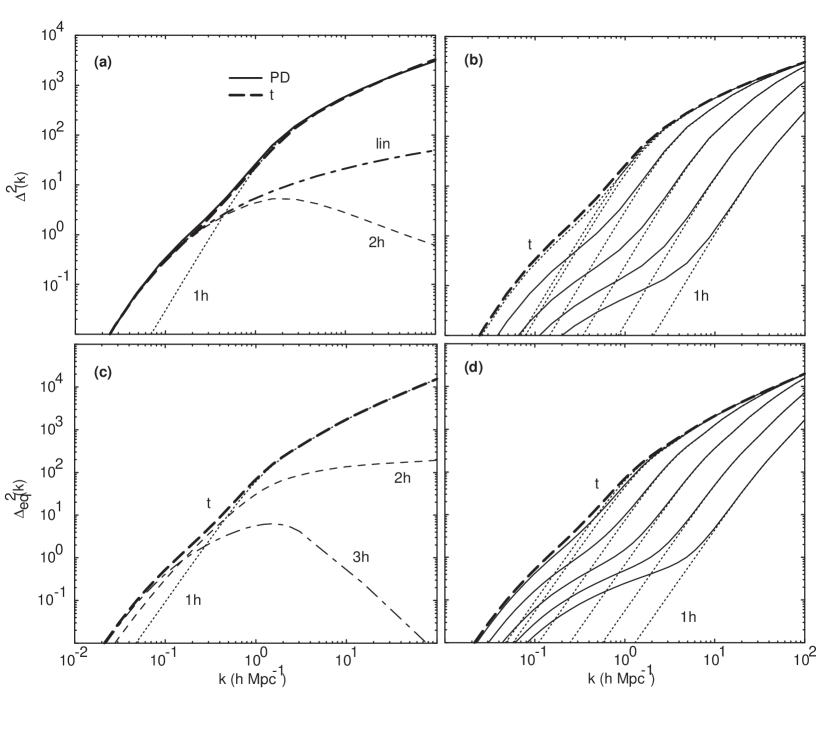
Figure 1.3: Present day dark matter density (a) power spectrum and (c) equilateral bispectrum under the halo prescription. The power spectrum shown in (a) is compared with the PD fitting function and the linear $P(k)$. We have decomposed the power spectrum and bispectrum to individual contributing terms under the halo approach. The mass cut off effects on the present day dark matter density power spectrum (b) and bispectrum (d) under the halo approach. From bottom to top, the maximum mass used in the calculation is $10^{11}$, $10^{12}$, $10^{13}$, $10^{14}$, $10^{15}$ and $10^{16}$ M${}_{\sun}$.

Mass Function

In order to describe the dark matter halo mass distribution, in general, we can consider two analytical forms commonly found in the literature. These are the Press-Schechter (PS; [Press & Schechter] 1974) and Sheth-Tormen (ST; [Sheth & Tormen] 1999) mass functions and are both parameterized by

$$\frac{dn}{dM}dM=\frac{\rho_{b}}{M}f(\nu)d\nu$$ (1.78)

with $f(\nu)$ taking the general form of

$$\nu f(\nu)=A\sqrt{\frac{2}{\pi}}\left[1+(a\nu^{2})^{-p}\right](a\nu)\exp\left(-a\nu^{2}/2\right)\,.$$ (1.79)

Here, $\nu=\delta_{c}/\sigma(M,z)$, where $\sigma(M,z)$ is the rms fluctuation within a top-hat filter at the virial radius corresponding to mass $M$, and $\delta_{c}$ is the threshold overdensity of spherical collapse.

The normalization $A$ in Eq. 1.79 is set by requiring the mass conservation, such that the average mass density from the mass function is same as the average mass density of the universe:

$$\int\frac{dn}{dM}\frac{M}{\rho_{b}}dM=\int f(\nu)d\nu=1\,,$$ (1.80)

and takes values of 0.5 and 0.383 when the PS $(p=0,a=1)$ or ST $(p=0.3,a=0.707)$ mass functions are used respectively. The two mass functions behave such that when $\nu$ is small, $\nu f(\nu)\propto\nu^{1.0}$ and $\propto\nu^{0.4}$ for PS and ST mass functions, respectively. Note that the difference in mass functions can be compensated by a difference in the concentration-mass relation (see, e.g., [Seljak] 2000; [Cooray & Hu] 2001a). Thus, we will simply use the PS mass function throughout here. We take the minimum mass to be $10^{3}$ M${}_{\sun}$ while the maximum mass is varied to study the effect of massive halos on lensing convergence statistics. In general, masses above $10^{16}$ M${}_{\sun}$ do not contribute to low order statistics due to the exponential decrease in the number density of such massive halos.

1.5 Dark Matter Power Spectrum and Bispectrum

In Fig. 1.3(a-b), we show the density field power spectrum today ($z=0$), written such that $\Delta^{2}(k)=k^{3}P(k)/2\pi^{2}$ is the power per logarithmic interval in wavenumber. In Fig 1.3(a), we show individual contributions from the single and double halo terms and a comparison to the non-linear power spectrum as predicted by the PD fitting function. In Fig. 1.3(b), we show the dependence of density field power as a function of maximum mass used in the calculation. Here, we show the power spectrum and bispectrum such that the concentration-mass formula is modified to match the PD fitting function with parameters as listed in under Eq. 1.70.

In general, the behavior of dark matter power spectrum due to halos can be understood in the following way. The linear portion of the dark matter power spectrum, $k<0.1$ h Mpc^-1, results from the correlation between individual dark matter halos and reflects the bias prescription. The fitting formulae of [Mo & White] (1996) adequately describes this regime for all redshifts. The mid portion of the power spectrum, around $k\sim 0.1-1$ h Mpc^-1 corresponds to the non-linear scale $M\sim M_{\star}(z)$, where the Poisson and correlated term contribute comparably. At higher $k$’s, the power arises mainly from the contributions of individual halos. Similarly, at the same high scales when $k\gtrsim$ few tens h Mpc^-1, the PD fitting function is not reliable due to resolution limit of the simulations from which the fitting function for the non-linear power spectrum was derived. In addition to the NFW profile, one can consider variants, however, with the freedom to change the concentration-mass relation, such variations do not produce recognizable differences in the power spectrum and the bispectrum (see, [Seljak] 2000 and [Cooray & Hu] 2001a for a discussion). We also refer the reader to [Seljak] 2000 for a discussion of the detailed properties of galaxy power spectra due to halos; we briefly discuss the subject of galaxy power spectra in § 1.7 using the PCSZ redshift-space galaxy power spectrum from [Hamilton & Tegmark] (2000).

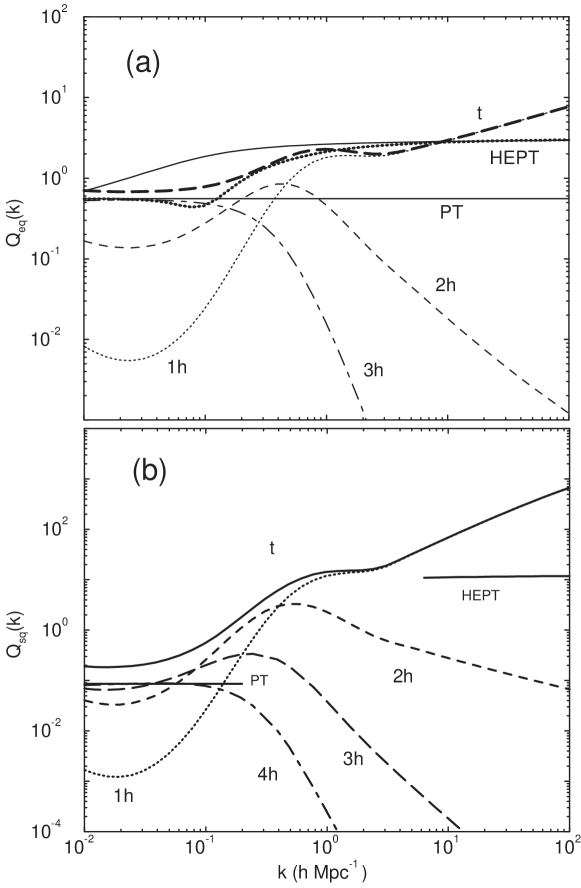
Figure 1.4: (a) $Q_{\rm eq}(k)$ and (b) $Q_{\rm sq}$ at present broken into individual contributions under the halo description and compared with second order perturbation theory (PT) and hyper-extended perturbation theory (HEPT). In (a), the thick dotted line shows the $Q_{\rm eq}$ based on the fitting function of [Scoccimarro & Couchman] (2000) that combines HEPT at small scales and PT at large scales. In (b), in the linear regime, the perturbation theory (PT) prediction is reproduced by the $4$ halo term which is only $\sim 1/2$ of the total. See text for a discussion of discrepancies.

Since the bispectrum generally scales as the square of the power spectrum, it is useful to define

$$\Delta_{\rm eq}^{2}(k)\equiv\frac{k^{3}}{2\pi^{2}}\sqrt{B(k,k,k)}\,,$$ (1.81)

which represents equilateral triangle configurations, and its ratio to the power spectrum

$$Q_{\rm eq}(k)\equiv{1\over 3}\left[{\Delta_{\rm eq}^{2}(k)\over\Delta^{2}(k)}\right]^{2}\,.$$ (1.82)

In second order perturbation theory,

$$Q_{\rm eq}^{\rm PT}=1-\frac{3}{7}\Omega_{m}^{-2/63}$$ (1.83)

and under hyper-extended perturbation theory (HEPT; [Scoccimarro & Frieman] 1999),

$$Q_{\rm eq}^{\rm HEPT}(k)=\frac{4-2^{n(k)}}{1+2^{n(k)+1}}\,,$$ (1.84)

which is claimed to be valid in the deeply nonlinear regime. Here, $n(k)$ is the linear power spectral index at $k$.

In Fig. 1.3(c-d), we show $\Delta_{\rm eq}^{2}(k)$ separated into its various contributions (c) and as a function of maximum mass (d). Since the power spectra and equilateral bispectra share similar features, it is more instructive to examine $Q_{\rm eq}(k)$ (see Fig. 1.4a). Here we also compare it with the second order perturbation theory (PT) and the HEPT prediction. In the halo prescription, $Q_{\rm eq}$ at $k\gtrsim 10k_{\rm nonlin}\sim 10h$Mpc^-1 arises mainly from the single halo term. We also show $Q_{\rm eq}(k)$ predicted by the fitting function of [Scoccimarro & Couchman] (2000) based on simulations in the range of $0.1\lesssim k\lesssim 3$ h Mpc^-1. This function is designed such that it converges to HEPT value at small scales and PT value at large scales. The HEPT prediction, however, falls short on smaller scales; further work with numerical simulations, especially at scales with $k\gtrsim 10$ h Mpc^-1, where the predictions based on HEPT and halo models differ, will be useful to distinguish between various clustering hypotheses (see, e.g., [Ma & Fry] 2000c). The scales where the two predictions significantly differ is unlikely to be probed by weak lensing observations as such scales only contribute at angular scales of few arcseconds ($l\sim 10^{4}$).

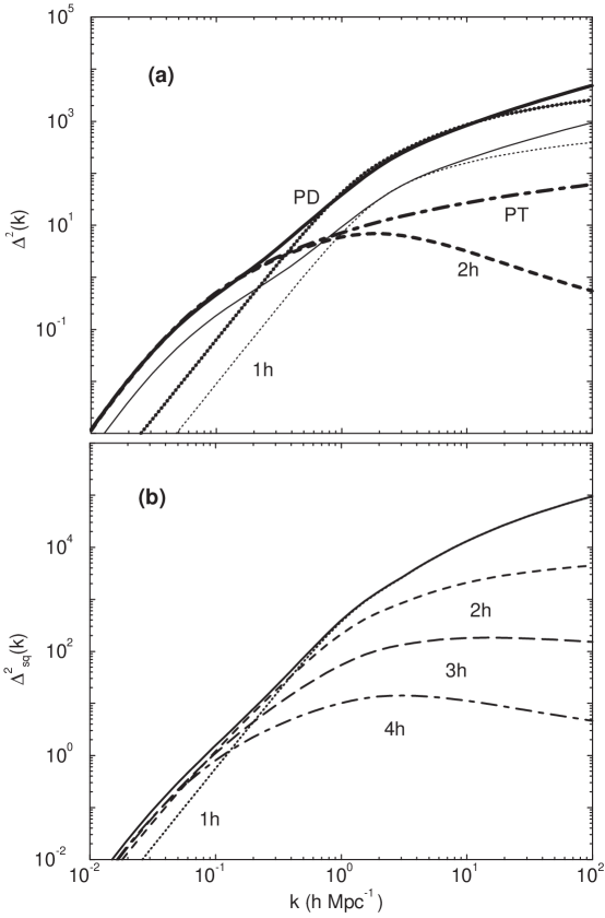
Figure 1.5: The dark matter power spectrum (a) and square-configuration trispectrum (b) broken into individual contributions under the halo description. The lines labeled ’PD’ shows the dark matter power spectrum under the [Peacock & Dodds] (1996) non-linear fitting function while the curve labeled ’PT’ is the linear dark matter power spectrum (at redshift of 0). In (a), we show the power spectrum at redshifts of 0 and 1. In (b), we show the square configuration trispectrum (see text). In both (a) and (b), at small scales the single halo term dominates while at large scales halo correlations contribute.

1.6 Dark Matter Power Spectrum Covariance

Following [Scoccimarro et al.] (1999), we can relate the trispectrum to the variance of the estimator of the binned power spectrum

$$\hat{P}_{i}={1\over V}\int_{{\rm s}i}{d^{3}k\over V_{{\rm s}i}}\delta^{*}(-{\bf k})\delta({\bf k})\,,$$ (1.85)

where the integral is over a shell in $k$-space centered around $k_{i}$, $V_{{\rm s}i}\approx 4\pi k_{i}^{2}\delta k$ is the volume of the shell and $V$ is the volume of the survey. Recalling that $\delta({\bf 0})\rightarrow V/(2\pi)^{3}$ for a finite volume,

$$C_{ij} \equiv \left<\hat{P}_{i}\hat{P}_{j}\right>-\left<\hat{P}_{i}\right>\left<\hat{P}_{j}\right>$$ (1.86)

$$= {1\over V}\left[{(2\pi)^{3}\over V_{{\rm s}i}}2P_{i}^{2}\delta_{ij}+T_{ij}\right]\,,$$

where

$$T_{ij} \equiv \int_{{\rm s}i}{d^{3}k_{i}\over V_{{\rm s}i}}\int_{{\rm s}j}{d^{3}k_{j}\over V_{{\rm s}j}}T({\bf k}_{i},-{\bf k}_{i},{\bf k}_{j},-{\bf k}_{j})\,.$$ (1.87)

Notice that though both terms scale in the same way with the volume of the survey, only the Gaussian piece necessarily decreases with the volume of the shell. For the Gaussian piece, the sampling error reduces to a simple root-N mode counting of independent modes in a shell. The trispectrum quantifies the non-independence of the modes both within a shell and between shells. Calculating the covariance matrix of the power spectrum estimates reduces to averaging the elements of the trispectrum across configurations in the shell. It is to the description of the trispectrum that we now turn.

1.6.1 Trispectrum

In Fig. 1.5(a), we show the logarithmic power spectrum $\Delta^{2}(k)=k^{3}P(k)/2\pi^{2}$ with contributions broken down to the $1h$ and $2h$ terms today and the $1h$ term at redshift of 1. Here, we use the concentration-mass relation as found by [Bullock et al] (2000) in their numerical simulations in the $\Lambda$CDM cosmology. We have taken the width of concentration-mass distribution to be $\sigma_{\rm lnc}=0.2$. Our prediction for the non-linear power spectrum is compared with the PD fitting function. The same prediction here with the concentration-mass relation from simulation and the one obtained by fitting for the PD function can be compared through Fig. 1.3(a). When compared to PD fitting function, and using results from numerical simulations for concentration, we find that there is an slight overprediction of power at scales corresponding to $1\lesssim k\lesssim 10$ h Mpc^-1 at redshifts of 0 and 1, and a more substantial underprediction at small scales with $k\gtrsim 10$ h Mpc^-1. Since the non-linear power spectrum has only been properly studied out to overdensities $\Delta^{2}\sim 10^{3}$ with numerical simulations it is unclear whether the small-scale disagreement is significant. Fortunately, it is on sufficiently small scales so as not to affect weak gravitational lensing observables.

For the trispectrum, and especially the contribution of trispectrum to the covariance, we are mainly interested in terms involving $T({\bf k}_{1},-{\bf k}_{1},{\bf k}_{2},-{\bf k}_{2})$, i.e. parallelograms which are defined by either the length $k_{12}$ or the angle between ${\bf k}_{1}$ and ${\bf k}_{2}$. For illustration purposes we will take $k_{1}=k_{2}$ and the angle to be $90^{\circ}$ (${\bf k}_{2}={\bf k}_{\perp}$) such that the parallelogram is a square. It is then convenient to define

$$\Delta^{2}_{\rm sq}(k)\equiv\frac{k^{3}}{2\pi^{2}}T^{1/3}({\bf k},-{\bf k},{\bf k}_{\perp},-{\bf k}_{\perp})\,,$$ (1.88)

such that this quantity scales roughly as the logarithmic power spectrum itself $\Delta^{2}(k)$. This spectrum is shown in Fig. 1.5(b) with the individual contributions from the 1h, 2h, 3h, 4h terms shown.

We test the sensitivity of our calculations to the width of the distribution in Fig. 1.6, where we show the ratio between single halo contribution, as a function of the concentration distribution width, to the halo term with a delta function distribution $\sigma_{\rm lnc}=0$. The fiducial value of the width suggested by simulations is $\sigma_{\rm lnc}=0.2$. As in the power spectrum the effect of increasing the width is to increase the amplitude at small scales due to the high concentration tail of the distribution. Notice that the width effect is stronger in the trispectrum than the power spectrum since the tails of the distribution are weighted more heavily in higher point statistics.

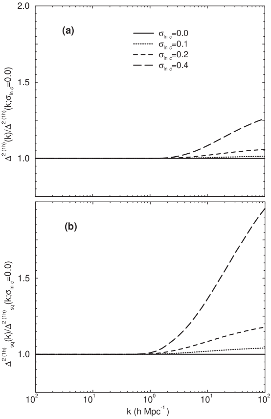
Figure 1.6: The ratio of the single halo term contribution to that for a concentration width $\sigma_{\ln c}\rightarrow 0$ for the (a) power spectrum and (b) trispectrum. The small scale behavior is increasingly sensitive to the high concentration tails for the higher order statistics.

To compare the specific scaling predicted by perturbation theory in the linear regime and the hierarchical ansatz in the deeply non-linear regime, it is useful to define the quantity

$$Q_{\rm sq}(k)\equiv\frac{T({\bf k},-{\bf k},{\bf k}_{\perp},-{\bf k}_{\perp})}{[8P^{2}(k)P(\sqrt{2}k)][4P^{3}(k)]}\,.$$ (1.89)

In the halo prescription, $Q_{\rm sq}$ at $k\gtrsim 10k_{\rm nonlin}\sim 10h$Mpc^-1 arises mainly from the single halo term. In perturbation theory $Q_{\rm sq}\approx 0.085$. The $Q_{\rm sq}$ does not approach the perturbation theory prediction as $k\rightarrow 0$ since that contribution appears only as one term in the 4 halo piece. Our model therefore does not recover the true trispectrum of the density field in the linear regime. The problem is that in modeling the density field with discrete objects, here halos, there is an error associated with shot noise. A more familiar example of the same effect comes from the use of galaxies as tracers of the dark matter density field. While this error appears large in the $Q_{\rm sq}$ statistic, it does not affect the calculations of the power spectrum covariance since in this regime, it is the Gaussian piece errors that dominate.

The hierarchical ansatz predicts that $Q_{\rm sq}=$ const. in the deeply non-linear regime. Its value is unspecified by the ansatz but is given as

$$Q_{\rm sq}^{\rm sat}=\frac{1}{2}\left[\frac{54-27\cdot 2^{n}+2\cdot 3^{n}+6^{n}}{1+6\cdot 2^{n}+3\cdot 3^{n}+6\cdot 6^{n}}\right]$$ (1.90)

under hyperextended perturbation theory (HEPT; [Scoccimarro & Frieman]). Here $n=n(k)$ is the linear power spectral index at $k$. As shown in Fig. 1.4(b), the halo model predicts $Q_{\rm sq}$ increases at high $k$. This behavior, also present at the three point level for the dark matter density field bispectrum, suggests disagreement between the halo approach and hierarchical clustering ansatz (see, [Ma & Fry] 2000b), though numerical simulations do not yet have enough resolution to test this disagreement. Fortunately the discrepancy is also outside of the regime important for lensing.

1.6.2 Further Tests of the Dark Matter Covariance

To further test the accuracy of our halo trispectrum, we compare dark matter correlations predicted by our method to those from numerical simulations by [Meiksin & White] (1999). For this purpose, we calculate the covariance matrix $C_{ij}$ from Eq. 1.87 with the bins centered at $k_{i}$ and volume $V_{{\rm s}i}=4\pi k_{i}^{2}\delta{k_{i}}$ corresponding to their scheme. We also employ the parameters of their $\Lambda$CDM cosmology and assume that the parameters that defined the halo concentration properties from our fiducial $\Lambda$CDM model holds for this cosmological model also. The physical differences between the two cosmological model are minor, though normalization differences can lead to large changes in the correlation coefficients.

$k$	0.06	0.07	0.09	0.11	0.14	0.17	0.21	0.25	0.31
0.06	1.00	0.06	0.12	0.18	0.25	0.30	0.33	0.34	0.33
0.07	(0.04)	1.00	0.10	0.19	0.30	0.37	0.41	0.42	0.41
0.09	(0.03)	(0.08)	1.00	0.16	0.29	0.40	0.47	0.48	0.48
0.11	(0.09)	(0.09)	(0.03)	1.00	0.28	0.43	0.54	0.58	0.57
0.14	(0.15)	(0.20)	(0.08)	(0.20)	1.00	0.43	0.58	0.69	0.70
0.17	(0.14)	(0.23)	(0.18)	(0.25)	(0.28)	1.00	0.59	0.74	0.78
0.21	(0.18)	(0.32)	(0.19)	(0.31)	(0.40)	(0.48)	1.00	0.75	0.84
0.25	(0.21)	(0.34)	(0.26)	(0.35)	(0.49)	(0.61)	(0.65)	1.00	0.86
0.31	(0.20)	(0.37)	(0.26)	(0.40)	(0.51)	(0.62)	(0.72)	(0.82)	1.00
$\sqrt{\frac{C_{ii}}{C_{ii}^{G}}}$	1.02	1.03	1.04	1.07	1.14	1.23	1.38	1.61	1.90

Table 1.1: Diagonal normalized covariance matrix of the binned dark matter density field power spectrum with $k$ values in units of h Mpc^-1. Upper triangle displays the covariance found under the halo model. Lower triangle (parenthetical numbers) displays the covariance found in numerical simulations by [Meiksin & White] (1999). Final line shows the fractional increase in the errors (root diagonal covariance) due to non-Gaussianity as calculated under the halo model.

In Table 1.1, we compare the predictions for the correlation coefficients

$$\hat{C}_{ij}={C_{ij}\over\sqrt{C_{ii}C_{jj}}}$$ (1.91)

with the simulations. Agreement in the off diagonal elements is typically better than $\pm 0.1$, even in the region where non-Gaussian effects dominate, and the qualitative features such as the increase in correlations across the non-linear scale are preserved.

A further test on the accuracy of the halo approach is to consider higher order real-space moments such as skewness and kurtosis. In [Cooray & Hu] (2000), we discussed the weak lensing convergence skewness under the halo model and found it to be in agreement with numerical predictions from [White & Hu] (1999). The fourth moment of the density field, under certain approximations, was calculated by [Scoccimarro et al.] (1999) using dark matter halos and was found to be in good agreement with N-body simulations. Given that density field moments have already been studied by [Scoccimarro et al.] (1999), we no longer consider them here other than to suggest that the halo model has provided, at least qualitatively, a consistent description better than any of the perturbation theory arguments.

1.7 From Dark Matter to Galaxies

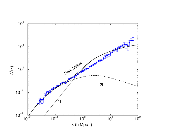
Figure 1.7: The PCSZ galaxy power spectrum compared to the dark matter power spectrum. The galaxy power spectrum comes from [Hamilton & Tegmark] (2000), and we have scaled the dark matter power spectrum with a linear scale-independent bias factor. At non-linear scales, the dark matter clustering cannot reproduce the galaxy power.

In Fig. 1.7, we show the redshift-space galaxy power spectrum from the PCSZ survey as derived by [Hamilton & Tegmark] (2000). For comparison, we show the non-linear dark matter power spectrum with the galaxy power spectrum scaled with a constant bias in the linear regime following the analysis given in [Hamilton & Tegmark] (2000). In the mildly to deeply non-linear regime, the galaxy power spectrum cannot be simply reproduced through an overall scaling of the non-linear dark matter power spectrum. This disagreement provides a strong argument against a scale independent bias for galaxy at all scales.

To understand the behavior of the galaxy power spectrum under the halo model, we follow discussions in [Seljak] (2000) and [Scoccimarro et al.] (2000). The basic idea here is that the galaxies can be considered as a tracer of the dark matter. Thus, its clustering properties inside a halo will simply follow the distribution of dark matter in that halo. Since the clustering measurements only involve the galaxies, one can relate the galaxy population in halos to the dark matter, as a function of the halo mass, through a relation that involves the mean number of galaxies per halo. This is essentially similar to the idea we presented to describe pressure, which involves a similar mean relation through the temperature-mass description for electrons in halos.

Following [Seljak] (2000), we describe the average number of galaxies per halo, $\left<N_{\rm gal}\right>$ in Eq. 1.44, such that

$$\left<N_{\rm gal}\right>=\left(\frac{M}{M_{\rm min}}\right)^{0.8}\\$$ (1.92)

where $M_{\rm min}$, the minimum dark matter halo mass in which a galaxy is found, is taken to be $5.3\times 10^{11}h^{-1}$ M${}_{\sun}$ for our fiducial $\Lambda$CDM cosmological model following [Benson et al.] (1999). The above relation is consistent with semi-analytical models, however, we ignore scatter in the observed distribution on the mean number of galaxies per halo. In addition to semi-analytic work, the above mean number of galaxies is consistent with the relation found by [Scoccimarro et al.] (2000) under the halo approach when compared to clustering of galaxies in the APM survey. The reason why the number of galaxies scales as $M^{0.8}$, instead of simply mass, can be understood by noting that the galaxy formation is suppressed in large mass halos due to the significantly higher cooling time when compared to the cooling times for gas in low mass halos. Thus, low mass halos, such as galaxy groups, have a higher efficiency for galaxy formation than high mass halos, such as massive clusters of galaxies. Such a mass dependent efficiency for galaxy formation can be easily used to explain the excess of entropy in galaxy clusters relative to smaller groups (see, e.g., [Bryan] 2000).

To calculate the 1-halo term of the galaxy power spectrum, in addition to the mean number of galaxies, one also require information on the second moment of the galaxy distribution. Using semi-analytic models, [Scoccimarro et al.] (2000), advocate

$$\left<N_{\rm gal}(N_{\rm gal}-1)\right>=\alpha(M)^{2}\left<N_{\rm gal}\right>^{2}$$ (1.93)

where $\alpha(M)$ is used to quantify the deviations from Poisson statistics.

In [Scoccimarro et al.] (2000), $\alpha(M)\sim log(M/10^{11}h^{-1}M_{\sun})^{0.5}$ out to a mass of $10^{13}$ $h^{-1}$ M${}_{\sun}$ while $\alpha(M)=1$ thereafter. Other variants to this approach are considered in [Seljak] (2000).

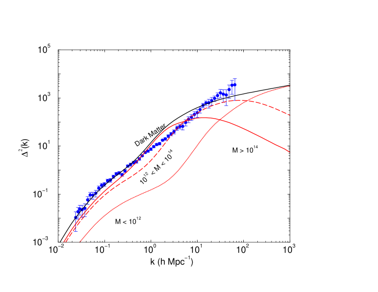
Figure 1.8: The non-linear dark matter power spectrum under the halo approach broken to contributions as a function of mass. The large scale power is produced by massive halos while the small scales power is produced by the small mass halos. The galaxy power spectrum is produced through appropriate scaling of the contributions to the dark matter power spectrum as a function of mass through the average number of galaxies vs. mass relation.

Using the information on the galaxy distribution within halos, the 2-halo and 1-halo terms for the galaxy power spectrum is

$$P^{2h}_{{\rm gal}}(k)=P^{\rm lin}(k)\left[\int dM\frac{d\bar{n}}{dM}b_{1}(M)\frac{\left<N_{\rm gal}\right>}{\bar{n}_{\rm gal}}y_{\delta}(k,M)\right]^{2}\,,$$ (1.94)

and

$$P^{1h}_{{\rm gal}}(k)=\left[\int dM\frac{d\bar{n}}{dM}\frac{\left<N_{\rm gal}(N_{\rm gal}-1)\right>}{\bar{n}_{\rm gal}^{2}}y_{\delta}(k,M)\right]^{2}\,,$$ (1.95)

respectively. With the the mean number of galaxies per halo, as a function of mass, the mean number density of galaxies can be written as an integral over the PS mass function

$$\bar{n}_{\rm gal}=\int dM\,\left<N_{\rm gal}\right>\frac{dn}{dM}(M,z)\,.$$ (1.96)

At large scales, since the galaxy power spectrum can be written as a simply scaling of the linear power spectrum

$$P_{{\rm gal}}(k)=b_{\rm gal}^{2}P^{\rm lin}(k),$$ (1.97)

we can write the galaxy bias at such linear scales as a mass weighted halo bias

$$b_{\rm gal}=\int dM\frac{d\bar{n}}{dM}b_{1}(M)\frac{\left<N_{\rm gal}\right>}{\bar{n}_{\rm gal}}\,.$$ (1.98)

With sufficient statistics, a measurement of the galaxy power spectrum at linear scales, as a function of galaxy type or environment, allows one to relate the observed bias to a mean mass of halos in which galaxies under study reside. It is likely that such studies can easily be carried out with wide-field surveys such as the Sloan Digital Sky Survey (SDSS).

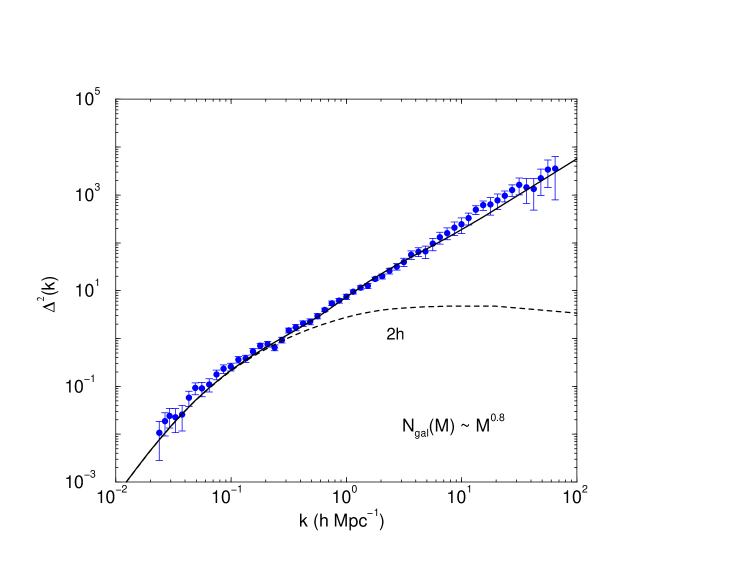
Figure 1.9: The PCSZ galaxy power spectrum produced through the mean number of galaxies as a function of mass relation. With appropriate scaling, the halo model produces the almost power law galaxy power spectrum measured in the PCSZ survey.

To construct the galaxy power spectrum, through the relation involving the mean number of galaxies as a function of mass, one essentially rescales the contribution to the dark matter power spectrum. The scaling through $N_{\rm gal}\sim M^{0.8}$ is such that one weighs the high mass end of dark matter halos relatively higher than the low mass end. In Fig. 1.8, we show the dark matter power spectrum such that contributions are separated as a function of mass. In Fig. 1.9, we show the prediction for the galaxy power spectrum, with parameters for the galaxy distribution as defined above. Note that the we have not tried to vary the parameters for the galaxy prescription so as to fit the PCSZ redshift-space galaxy power spectrum. Given that there are still discrepancies between this prediction and the measured galaxy power spectrum, it is likely that some variants of the parameters can lead to a better model. We leave these detailed issues to future studies, since we are primarily interested in here for a simple description of galaxy power spectrum under the halo approach.

1.8 Discussion

Even though the dark matter halo formalism provides a physically motivated means for calculating the statistics of the dark matter density field, there are several limitations of the approach that should be borne in mind when interpreting the results.

The approach assumes all halos to be spherical with a single profile shape. Any variations in the profile through halo mergers and resulting substructure can affect the power spectrum and higher order correlations. Also, real halos are not perfectly spherical which affects the configuration dependence of the bispectrum. Furthermore, there are parameter degeneracies in the formalism that prevent a straightforward interpretation of observations in terms of halo properties. For example, one might think that the power spectrum and bispectrum can be used to measure any mean deviation from the assumed NFW profile form. However as pointed out by [Seljak] (2000), changes in the slope of the inner profile can be compensated by changing the concentration as a function of mass; this degeneracy is also preserved in the bispectrum.

In the case of the trispectrum and power specrum covariance, we have attempted to include variations in the halo profiles with the addition of a distribution function for concentration parameter based on results from numerical simulations. Also, for the calculation involving dark matter trispectrum and covariance, we have not modified the concentration-mass relation to fit the PD non-linear power spectrum, but rather have taken results directly from simulations as inputs. Though we have partly accounted for halo profile variations, the assumption that halos are spherical is likely to affect detailed results on the configuration dependence of the bispectrum and trispectrum.

We do not expect these issues to affect our qualitative results. If this technique is to be used for precision studies of cosmological parameters, however, more work will be required in testing it quantitatively against simulations. Studies by [Ma & Fry] (2000a) show that the bispectrum predictions of the halo formalism are in good agreement with simulations, at least when averaged over configurations. [Scoccimarro et al.] (2000) find that there are discrepancies at the $\sim 20-30\%$ level in the mildly non-linear regime that show up most markedly in the configuration dependence; uncertainties in the mass function, with respect to the mass functions produced in simulations, also produce variations at this level. The replacement of individual halos found in numerical simulations with synthetic smooth halos with NFW profiles by [Ma & Fry] (2000b) show that the smooth profiles can regenerate the measured power spectrum and bispectrum in simulations. This agreement, at least at scales less than 10$k_{\rm nonlin}$, suggests that mergers and substructures may not be important at such scales.

The agreement between the power spectrum and bispectrum for a given halo prescription is also significant in that, as we shall see, the two statistics weight high mass halos very differently. The agreement serves as a test that the halo prescription correctly captures the halo mass dependence of the statistics. We conclude that the halo model is useful in that it provides a means to study the halo mass dependence of two, three and four point statistics and an approximate means to bridge the gap between the linear regime where PT is valid and the non-linear regime where extensions such as HEPT can be used.

In the deeply non-linear regime (here $k\gtrsim 10h$Mpc^-1) there are qualitative differences between the halo predictions and HEPT. Unfortunately, current state-of-the-art simulations do not have the resolution to address the differences [Scoccimarro et al.] (2000). For weak lensing purposes, the differences are less relevant since in the deeply non-linear regime shot-noise from the intrinsic ellipticities of the galaxies will likely dominate. We will now discuss applications of the halo model to weak gravitational lensing.

Chapter 2 Weak Gravitational Lensing

2.1 Introduction

Weak gravitational lensing of faint galaxies probes the distribution of matter along the line of sight. Lensing by large-scale structure (LSS) induces correlation in the galaxy ellipticities at the percent level (e.g., [Blandford et al] 1991; [Miralda-Escudé] 1991; [Kaiser] 1992). Though challenging to measure, these correlations provide important cosmological information that is complementary to that supplied by the cosmic microwave background and potentially as precise (e.g., [Jain & Seljak] 1997; [Bernardeau et al] 1997; [Kaiser] 1998; [Schneider et al] 1998; [Hu & Tegmark] 1999; [Cooray] 1999; [Van Waerbeke et al] 1999; see [Bartelmann & Schneider] 2000 for a recent review). Indeed several recent studies have provided the first clear evidence for weak lensing in so-called blank fields (e.g., [Van Waerbeke et al] 2000; [Bacon et al] 2000; [Wittman et al] 2000; [Kaiser et al] 2000), though more work is clearly needed to understand even the statistical errors (e.g. [Cooray et al] 2000b).

Weak lensing surveys are currently limited to small fields which may not be representative of the universe as a whole, owing to sample variance. In particular, rare massive objects can contribute strongly to the mean power in the shear or convergence but not be present in the observed fields. The problem is compounded if one chooses blank fields subject to the condition that they do not contain known clusters of galaxies. The objective with halo approach is to (1) quantify these effects and to understand what fraction of the total convergence power spectrum and higher order correlations arise from lensing by individual massive clusters as a function of scale and (2) understand how the sample variance effects affect the cosmological interpretation of weak lensing convergence observations through galaxy shear data. In this chapter, we address the first issue while the second issue is discussed in the next chapter.

Given that weak gravitational lensing results from the projected mass distribution, the statistical properties of weak lensing convergence reflect those of the dark matter. Non-linearities in the mass distribution induce non-Gaussianity in the convergence distribution. These non-Gaussianities contribute to the covariance of power spectrum measurements, especially in the case when observations are limited to a finite field of view and the measurements are binned in multipole space. Here, we present an analytical estimate on the covariance of binned power spectrum, based on the non-Gaussian contribution. The calculation of the full convergence covariance requires detailed knowledge of the dark matter density bispectrum, which can be obtain analytically through perturbation theory (e.g., [Bernardeau et al] 1997) or numerically through simulations (e.g., [Jain et al] 2000; [White & Hu] 1999). Perturbation theory, however, is not applicable at all scales of interest, while numerical simulations are limited by computational expense to a handful of realizations of cosmological models with modest dynamical range. Here, we use a recent popular approach to obtain the density field bispectrum analytically by describing the underlying three point correlations as due to contributions from (and correlations between) individual dark matter halos.

Techniques for studying the dark matter density field through halo contributions have recently been developed ([Seljak] 2000; [Ma & Fry] 2000b; [Scoccimarro et al.] 2000) and applied to two-point and three-point lensing statistics ([Cooray et al] 2000b; [Cooray & Hu] 2000). The critical ingredients are: a mass function for the halo distribution, such as the Press-Schechter (PS; [Press & Schechter] 1974) or Sheth-Tormen (ST; [Sheth & Tormen] 1999) mass function; a profile for the dark matter halo, e.g., the profile of [Navarro et al] (1996; NFW), and a description of halo biasing ([Mo et al.] 1997; extensions in [Sheth & Lemson] 1999 and [Sheth & Tormen] 1999). The dark matter halo approach provides a physically motivated method to calculate the correlation functions. Since lensing probes scales ranging from linear to deeply non-linear, this is an important advantage over perturbation-theory calculations.

Figure 2.1: Weak lensing convergence (a) power spectrum and (c) bispectrum under the halo description. Also shown in (a) is the prediction from the PD nonlinear power spectrum fitting function. We have separated individual contributions under the halo approach to weak lensing angular power spectrum and bispectrum. The mass cut off effects on the weak lensing convergence power spectrum (d) and bispectrum (d). The maximum mass used is same as in Fig. 1.3(b & d). We have assumed that all sources are at $z_{s}\ =1$.

2.2 Convergence Power Spectrum

The angular power spectrum of the convergence is defined in terms of the multipole moments $\kappa_{lm}$ as

$$\left<\kappa_{lm}^{*}\kappa_{l^{\prime}m^{\prime}}\right>=C_{l}^{\kappa}\delta_{ll^{\prime}}\delta_{mm^{\prime}}\,.$$ (2.1)

$C_{l}$ is numerically equal to the flat-sky power spectrum in the flat sky limit. It is related to the dark matter power spectrum by ([Kaiser] 1992; 1998)

$$C^{\kappa}_{l}=\int dr\frac{W^{\rm lens}(r)^{2}}{d_{A}^{2}}P^{\rm t}\left(\frac{l}{d_{A}};r\right)\,,$$ (2.2)

where $r$ is the comoving distance and $d_{A}$ is the angular diameter distance. When all background sources are at a distance of $r_{s}$, the weight function becomes

$$W^{\rm lens}(r)=\frac{3}{2}\Omega_{m}\frac{H_{0}^{2}}{c^{2}a}\frac{d_{A}(r)d_{A}(r_{s}-r)}{d_{A}(r_{s})}\,;$$ (2.3)

for simplicity, we will assume $r_{s}=r(z_{s}=1)$ throughout. In deriving Eq. 2.2, we have used the Limber approximation ([Limber] 1954) by setting $k=l/d_{A}$ and the flat-sky approximation. A potential problem in using the Limber approximation is that we implicitly integrate over the unperturbed photon paths (Born approximation). The Born approximation has been tested in numerical simulations by [Jain et al] (2000; see their Fig. 7) and found to be an excellent approximation for the two point statistics. The same approximation can also be tested through lens-lens coupling involving lenses at two different redshifts. For higher order correlations, analytical calculations in the mildly non-linear regime by [Van Waerbeke et al] (2000b; also, [Bernardeau et al] 1997; [Schneider et al] 1998) indicate that corrections are again less than a few percent. Thus, our use of the Limber approximation by ignoring the lens-lens coupling is not expected to change the final results significantly.

In Fig. 2.1(a), we show the convergence power spectrum of the dark matter halos compared with that predicted by the [Peacock & Dodds] (1996) power spectrum. The lensing power spectrum due to halos has the same behavior as the dark matter power spectrum. At large angles ($l\lesssim 100$), the correlations between halos dominate. The transition from linear to non-linear is at $l\sim 500$ where halos of mass similar to $M_{\star}(z)$ contribute. The single halo contributions start dominating at $l>1000$. When $l\gtrsim$ few thousand, at small scales corresponding to deeply non-linear regime, the intrinsic correlations between individual background galaxy shapes can complicate the accurate recovery of lensing signal ([Croft & Metzler] 2000; [Heavens et al.] 2000; [Catelan et al] 2000). Therefore, it is unlikely that the lensing observations can be used to test various clustering models that are relevant to such non-linear regimes.

As shown in Fig. 2.1(b), and discussed in [Cooray et al] (2000b), if there is a lack of massive halos in the observed fields convergence measurements will be biased low compared with the cosmic mean. The lack of massive halos affect the single halo contribution more than the halo-halo correlation term, thereby changing the shape of the total power spectrum in addition to decreasing the overall amplitude. Since the lensing power spectrum is simply a projected measure of the dark matter power spectrum, the variations in the weak lensing angular power spectra are consistent with the behavior observed in the dark matter power spectrum.

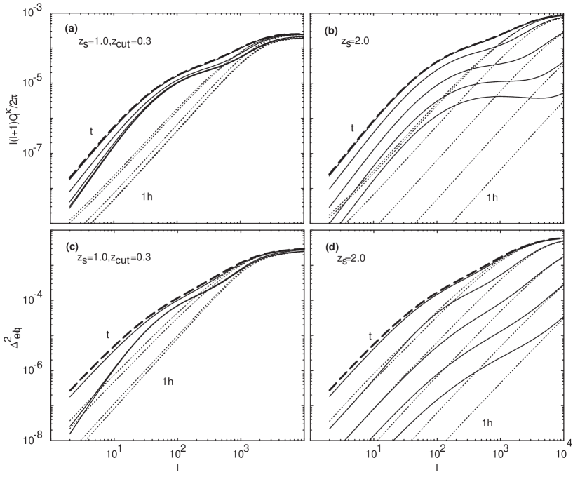
Figure 2.2: Weak lensing convergence spectra under the halo description for sources at $z_{s}=1$ with a mass cut off only applied to halos at $z_{c}=z<0.3$ and for source $z_{s}=2$ with mass cut off to the same redshift: (a) & (b) angular power spectrum and (c) & (d) Equilateral bispectrum. The mass cuts are the same as in Fig. 1.3(b & d). A significant fraction of the effect comes from rare massive halos at high redshift.

It is interesting to study the origin of this result in terms of the physical parameters to see how they depend on assumptions. The lensing convergence weight function (Eq. 2.3) peaks at half the angular diameter distance to background sources, which for our fiducial $\Lambda$CDM model with sources at $z_{s}=1$ corresponds to $z\approx 0.4$ with the growth of structures shifting this peak redshift to a slightly lower value. In Fig. 2.2(a & c), we show the result of the mass cuts where only those halos for which $z<0.3$ and $M<M_{\rm cut}$ are excluded. Note that the sensitivity to the mass threshold is reduced indicating that a substantial fraction of the effect comes from rare massive halos at high redshift. As shown in Fig. 2.2(b & d) when $z_{s}=2$, changing the source redshift therefore does not affect the results qualitatively.

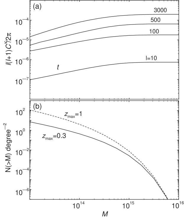
Figure 2.3: (a) Total lensing convergence $C_{\kappa}^{\rm tot}$ as a function of maximum mass for several $l$-values and sources at $z_{s}=1$. As shown, contributions from halos with masses $>10^{15}$ $M_{\sun}$ are negligible. (b) Surface density of halo masses as a function of minimum mass using PS formalism out to $z_{\rm max}=0.3$ and $z_{\rm max}=1$. This determines the survey area needed to ensure a fair sample of halos greater than a given mass.

In Fig. 2.3(a), we show the dependence of $C_{\kappa}$, for several $l$ values. If halos $<10^{15}$ $M_{\sun}$ are well represented in a survey, then the power spectrum will track the LSS convergence power spectrum for all $l$ values of interest. The surface number density of halos determines how large a survey should be to possess a fair sample of halos of a given mass. We show this in Fig. 2.3(b) as predicted by PS formalism for our fiducial cosmological model for halos out to ($z=0.3$ and $z=1.0$). Since the surface number density of $>10^{15}M_{\sun}$ halos out to a redshift of 0.3 and 1.0 is $\sim$ 0.03 and 0.08 degree^-2 respectively, a survey of order $\sim$ 30 degree² should be sufficient to contain a fair sample of the universe for recovery of the full LSS convergence power spectrum.

One caveat is that mass cuts may affect the higher moments of the convergence differently so that a fair sample for a quantity such as skewness will require a different survey strategy. From numerical simulations ([White & Hu] 1999), we know that $S_{3}\equiv\left<\kappa^{3}\right>/\left<\kappa^{2}\right>^{2}$ shows substantial sample variance, implying that it may be dominated by rare massive halos. As we find later, when calculated using density field bispectrum constructed using dark matter halos, the skewness decreased by a factor of $\sim$ 10 with a mass cut off at $\sim$ $10^{13}$ M${}_{\sun}$ at an angular scale of $10^{\prime}$ from the maximum value with masses out to $\sim$ 10¹⁶ M${}_{\sun}$. We will discuss issues related to non-Gaussianities in the next section.

While upcoming wide-field weak lensing surveys, such as the MEGACAM experiment at Canada-France-Hawaii Telescope ([Boulade et al] 1998), and the proposed wide field survey by Tyson et al. (2000, private communication) will cover areas up to $\sim$ 30 degree² or more, the surveys that have been so far published, e.g., [Wittman et al] (2000), only cover at most 4 degree² in areas without known clusters. The observed convergence in these fields should be biased low compared with the mean and vary widely from field to field due to sample variance from the Poisson contribution of the largest mass halos in the fields, which are mainly responsible for the sample variance below $10^{\prime}$ (see [White & Hu] 1999).

Our results can also be used proactively. If properties of the mass distribution such as the maximum mass halo in the observed lensing fields are known, say through prior optical, X-ray, SZ or even internally in the lensing observations (see [Kruse & Schneider] 1999), one can make a fair comparison of the observations to theoretical model predictions with a mass cut off in our formalism. Even for larger surveys, the identification and extraction of large halo contributions can be beneficial: most of the sample variance in the fields will be due to rare massive halos. The dependence of massive halos in producing a large non-Gaussian signal can also be used to identify their presence and perhaps correct the possible non-fair sampling of observing fields and variance of convergence measurement. A reduction in the sample variance increases the precision with which the power spectrum can be measured and hence the cosmological parameters upon which it depends. In the next Chapter, we will address the effect on cosmological parameters due to non-Gaussianities and the associated sample variance.

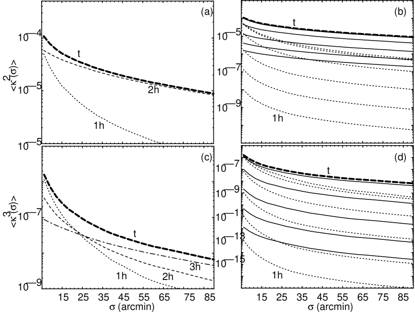
Figure 2.4: Moments of the convergence field as a function of top-hat smoothing scale $\sigma$. (a) Second moment broken into individual contributions. (b) Mass cut off effects on the second moments. (a) Third moment broken into individual contributions. (b) Mass cut off effects on the third moments. The mass cuts are the same as in Fig. 1.3.

In the case of the two point function, one can also consider the second moment, or variance, in addition to the power spectrum. The variance of a map smoothed with a window is related to the power spectrum by

$$\left<\kappa^{2}(\sigma)\right>={1\over 4\pi}\sum_{l}(2l+1)C_{l}^{\kappa}W_{l}^{2}(\sigma)\,.$$ (2.4)

where $W_{l}$ are the multipole moments (or Fourier transform in a flat-sky approximation) of the window. For simplicity, we will choose a window which is a two-dimensional top hat in real space with a window function in multipole space of $W_{l}(\sigma)=2J_{1}(x)/x$ with $x=l\sigma$.

In Fig. 2.4(a-b), we show the second moment as a function of smoothing scale $\sigma$. Here, we have considered angular scales ranging from 5^′ to 90^′, which are likely to be probed by ongoing and upcoming weak lensing experiments. As shown, most of the contribution to the second moment comes from the double halo correlation term and is mildly affected by a mass cut off.

Figure 2.5: The bispectrum configuration dependence $R_{l_{1}l_{2}}^{l_{3}}$ as a function of $l_{1}$ and $l_{2}$ with $l_{3}=1000$. Due to triangular conditions associated with $l$’s, only the upper triangular region in $l_{1}$-$l_{2}$ space contribute to the bispectrum.

2.3 Convergence Bispectrum

The angular bispectrum of the convergence is defined as

$$\left<\kappa_{l_{1}m_{1}}\kappa_{l_{2}m_{2}}\kappa_{l_{3}m_{3}}\right>=\left(\begin{array}[]{ccc}l_{1}&l_{2}&l_{3}\\ m_{1}&m_{2}&m_{3}\end{array}\right)B_{l_{1}l_{2}l_{3}}^{\kappa}\,,$$ (2.5)

where

$$\kappa(\hat{\bf n})=\sum\kappa_{lm}Y_{l}^{m}(\hat{\bf n})\,,$$ (2.6)

with spherical moments of the convergence field defined such that

$$\kappa_{lm} = i^{l}\int\frac{d^{3}{\bf k}}{2\pi^{2}}\delta_{\delta}({\bf k})I_{l}^{\rm lens}(k)Y_{l}^{m}(\hat{{\bf k}})\,,$$

$$I_{l}^{\rm lens}(k) = \int drW^{\rm lens}(k,r)j_{l}(kr)\,,$$ (2.7)

where $W(k,r)$ is the source function associated with weak lensing (see, Eq. 2.3). Here, we have simplified using the Rayleigh expansion of a plane wave

$$e^{i{\bf k}\cdot\hat{\bf n}r}=4\pi\sum_{lm}i^{l}j_{l}(kr)Y_{l}^{m\ast}(\hat{\bf k})Y_{l}^{m}(\hat{\bf n})\,.$$ (2.8)

The bispectrum can be written through

$$\left<\kappa_{l_{1}m_{1}}\kappa_{l_{2}m_{2}}\kappa_{l_{3}m_{3}}\right>=i^{l_{1}+l_{2}+l_{3}}$$ (2.9)

$$\times \int\frac{d^{3}{\bf k}_{1}}{2\pi^{2}}\int\frac{d^{3}{\bf k}_{2}}{2\pi^{2}}\int\frac{d^{3}{\bf k}_{3}}{2\pi^{2}}\left<\delta_{\delta}({\bf k}_{1})\delta_{\delta}({\bf k}_{2})\delta_{\delta}({\bf k}_{3})\right>$$

$$\times I_{l}^{\rm lens}(k_{1})I_{l}^{\rm lens}(k_{2})I_{l}^{\rm lens}(k_{3})Y_{l_{1}}^{m_{1}}(\hat{{\bf k}_{1}})Y_{l_{2}}^{m_{2}}(\hat{{\bf k}_{2}})Y_{l_{3}}^{m_{3}}(\hat{{\bf k}_{3}})\,,$$

and can be simplified further by using the bispectrum of density fluctuations

$$\left<\kappa_{l_{1}m_{1}}\kappa_{l_{2}m_{2}}\kappa_{l_{3}m_{3}}\right>=i^{l_{1}+l_{2}+l_{3}}\int\frac{d^{3}{\bf k}_{1}}{2\pi^{2}}\int\frac{d^{3}{\bf k}_{2}}{2\pi^{2}}\int\frac{d^{3}{\bf k}_{3}}{2\pi^{2}}$$ (2.10)

$$\times (2\pi)^{3}B_{\delta}(k_{1},k_{2},k_{3})\delta_{D}({\bf k}_{123})$$

$$\times I_{l}^{\rm lens}(k_{1})I_{l}^{\rm lens}(k_{2})I_{l}^{\rm lens}(k_{3})Y_{l_{1}}^{m_{1}}(\hat{{\bf k}_{1}})Y_{l_{2}}^{m_{2}}(\hat{{\bf k}_{2}})Y_{l_{3}}^{m_{3}}(\hat{{\bf k}_{3}})\,,$$

the expansion of a delta function

$$\delta_{D}({\bf k}_{123})=\int\frac{d^{3}{\bf x}}{(2\pi)^{3}}e^{i{\bf x}\cdot({\bf k}_{1}+{\bf k}_{2}+{\bf k}_{3})}\,,$$ (2.11)

and the Rayleigh expansion (Eq. 2.8), to write

$$\left<\kappa_{l_{1}m_{1}}\kappa_{l_{2}m_{2}}\kappa_{l_{3}m_{3}}\right>=\frac{2^{3}}{\pi^{3}}\int k_{1}^{2}dk_{1}\int k_{2}^{2}dk_{2}\int k_{3}^{2}dk_{3}$$ (2.12)

$$\times B_{\delta}(k_{1},k_{2},k_{3})I_{l}^{\rm lens}(k_{1})I_{l}^{\rm lens}(k_{2})I_{l}^{\rm lens}(k_{3})$$

$$\times \int x^{2}dxj_{l_{1}}(k_{1}x)j_{l_{2}}(k_{2}x)j_{l_{3}}(k_{3}x)\int d{\bf\hat{x}}Y_{l_{1}}^{m_{1}}({\bf\hat{x}})Y_{l_{2}}^{m_{2}}({\bf\hat{x}})Y_{l_{3}}^{m_{3}}({\bf\hat{x}})\,.$$

Here, the density bispectrum should be understood as arising from the full unequal time correlator

$$\left<\delta_{\delta}({\mathbf{k}}_{1};r_{1})\delta_{\delta}({\mathbf{k}}_{2};r_{2})\delta_{\delta}({\mathbf{k}}_{3};r_{3})\right>\,,$$ (2.13)

where the temporal coordinate is introduced to the source functions through individual $I_{l}^{\rm lens}$’s.

Using the Gaunt integral

$$\int d\hat{\bf n}Y_{l_{1}}^{m_{1}}Y_{l_{2}}^{m_{2}}Y_{l_{3}}^{m_{3}}=\sqrt{\prod_{i=1}^{3}(2l_{i}+1)\over 4\pi}\left(\begin{array}[]{ccc}l_{1}&l_{2}&l_{3}\\ 0&0&0\end{array}\right)\left(\begin{array}[]{ccc}l_{1}&l_{2}&l_{3}\\ m_{1}&m_{2}&m_{3}\end{array}\right)\,,$$ (2.18)

(2.19)

we can write the convergence bispectrum as

$$B^{\kappa}_{l_{1}l_{2}l_{3})} = \sum_{m_{1}m_{2}m_{3}}\left(\begin{array}[]{ccc}l_{1}&l_{2}&l_{3}\\ m_{1}&m_{2}&m_{3}\end{array}\right)\left<\kappa_{l_{1}m_{1}}\kappa_{l_{2}m_{2}}\kappa_{l_{3}m_{3}}\right>$$ (2.22)

$$= \sqrt{\frac{\prod_{i=1}^{3}(2l_{i}+1)}{4\pi}}\left(\begin{array}[]{ccc}l_{1}&l_{2}&l_{3}\\ 0&0&0\end{array}\right)b_{l_{1},l_{2},l_{3}}\,,$$ (2.25)

with

$$b_{l_{1},l_{2},l_{3}}=\frac{2^{3}}{\pi^{3}}\int k_{1}^{2}dk_{1}\int k_{2}^{2}dk_{2}\int k_{3}^{2}dk_{3}B_{\delta}(k_{1},k_{2},k_{3})$$

$$\times I^{\rm lens}_{l_{1}}(k_{1})I^{\rm lens}_{l_{2}}(k_{2})I^{\rm lens}_{l_{3}}(k_{3})\int x^{2}dxj_{l_{1}}(k_{1}x)j_{l_{2}}(k_{2}x)j_{l_{3}}(k_{3}x)\,.$$

In general, the calculation of $b_{l_{1},l_{2},l_{3}}$ involves seven integrals involving the mode coupling integral and three integrals involving distances and Fourier modes, respectively. For efficient calculational purposes, we can simplify further by using the Limber approximation. Here, we employ a version based on the completeness relation of spherical Bessel functions (see, [Cooray & Hu] 2000 for details)

$$\int dkk^{2}F(k)j_{l}(kr)j_{l}(kr^{\prime})\approx{\pi\over 2}d_{A}^{-2}\delta^{\rm D}(r-r^{\prime})F(k)\big{|}_{k={l\over d_{A}}}\,,$$ (2.27)

where the assumption is that $F(k)$ is a slowly-varying function. This is in fact the well known Limber approximation under the weak coupling approximation (see, [Hu & White] 1996). Under this assumption, the contributions to the bispectrum come only from correlations at equal time surfaces.

Applying this to the integrals involving $k_{1}$, $k_{2}$ and $k_{3}$ allows us to write the angular bispectrum of lensing convergence as

$$B_{l_{1}l_{2}l_{3}}^{\kappa} = \sqrt{\prod_{i=1}^{3}(2l_{i}+1)\over 4\pi}\left(\begin{array}[]{ccc}l_{1}&l_{2}&l_{3}\\ 0&0&0\end{array}\right)$$ (2.30)

$$\times \left[\int dr{[W^{\rm lens}(r)]^{3}\over d_{A}^{4}}B_{\delta}\left({l_{1}\over d_{A}},{l_{2}\over d_{A}},{l_{3}\over d_{A}};r\right)\right]\,.$$ (2.31)

The more familiar flat-sky bispectrum is simply the expression in brackets ([Hu] 2000b). The basic properties of Wigner-3$j$ symbol can be found in [Cooray & Hu] (2000).

Similar to the density field bispectrum, we define

$$\Delta^{2}_{{\rm eq}l}=\frac{l^{2}}{2\pi}\sqrt{B^{\kappa}_{lll}}\,,$$ (2.32)

involving equilateral triangles in $l$-space.

In Fig. 2.1(b), we show $\Delta^{2}_{{\rm eq}l}$. The general behavior of the lensing bispectrum can be understood through the individual contributions to the density field bispectrum: at small multipoles, the triple halo correlation term dominates, while at high multipoles, the single halo term dominates. The double halo term contributes at intermediate $l$’s corresponding to angular scales of a few tens of arcminutes. The variations in the weak lensing bispectrum as a function of maximum mass is shown in Fig. 2.1(d). Here, again, the variations and consistent with the behavior seen in dark matter bispectrum and produce qualitatively consistent results regardless of the exact halo profile or mass function.

2.3.1 Skewness

As discussed in the case of the second moment, it is likely that the first measurements of higher order correlations in lensing would be through real space statistics. Thus, in addition to the bispectrum, we also consider skewness which is associated with the third moment of the smoothed map (c.f. Eq. [2.4])

$$\left<\kappa^{3}(\sigma)\right> = {1\over 4\pi}\sum_{l_{1}l_{2}l_{3}}\sqrt{\prod_{i=1}^{3}(2l_{i}+1)\over 4\pi}\left(\begin{array}[]{ccc}l_{1}&l_{2}&l_{3}\\ 0&0&0\end{array}\right)$$

$$\times B_{l_{1}l_{2}l_{3}}^{\kappa}W_{l_{1}}(\sigma)W_{l_{2}}(\sigma)W_{l_{3}}(\sigma)\,.$$

We then construct the skewness as

$$S_{3}(\sigma)=\frac{\left<\kappa^{3}(\sigma)\right>}{\left<\kappa^{2}(\sigma)\right>^{2}}\,.$$ (2.37)

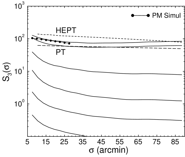
Figure 2.6: The skewness, $S_{3}(\sigma)$, as a function of angular scale. Shown here is the skewness values with varying maximum mass as in Fig. 1.3(c-d). For comparison, we also show skewness values as measured in particle-mesh (PM) simulations of [White & Hu] (1999), as predicted by hyper-extended perturbation theory (HEPT; dashed line) and second-order perturbation theory (PT; long-dashed line).

The effect of the mass cut off is dramatic in the third moment. As shown in Fig 2.4(c-d), most of the contributions to the third moment come from the single halo term, with those involving halo correlations contributing significantly only at angular scales greater than $\sim$ 25^′. With a mass cut off, the total third moment decreases rapidly and is suppressed by more than three orders of magnitude when the maximum mass drops to $10^{13}$ M${}_{\sun}$. The skewness only saturates when the maximum mass is raised to a few times $10^{15}$ M${}_{\sun}$. Even though a small change in the maximum mass does not greatly change the convergence power spectrum (Fig. 3 of [Cooray et al] 2000b), the third moment, or the bispectrum, is strongly sensitive to the rarest or most massive dark matter halos.

In Fig. 2.6 we plot the skewness as a function of maximum mass, ranging from $10^{11}$ to $10^{16}$ M${}_{\sun}$. Our total maximum skewness agrees with what is predicted by numerical particle mesh simulations ([White & Hu] 1999) and yields a value of $\sim$ 116 at 10^′. However, it is lower than predicted by HEPT arguments and simulations of [Jain et al] (2000), which suggest a skewness of $\sim$ 140 at angular scales of 10^′. The skewness based on second-order PT is factor of $\sim$ 2 lower than the maximum skewness predicted by halo calculation. As shown, the PT skewness decreases slightly from angular scales of few arcminutes to 90^′ and increases thereafter. Our halo based calculation of skewness differs from both [Hui] (1999) and [Bernardeau et al] (1997) as these authors used HEPT and PT respectively to calculate lensing skewness.

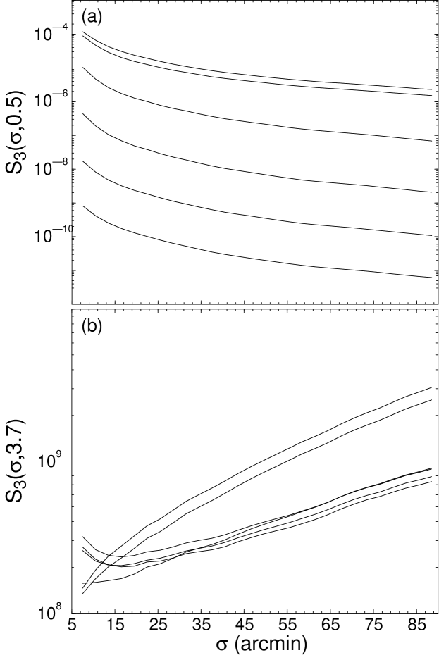
Figure 2.7: Generalized skewness statistic $S_{3}(\sigma,m)$. (a) $m=1/2$ following [Jain et al] (2000). (b) $m=3.7$ chosen to minimize the mass cut off dependence.

The effect of maximum mass on the skewness is interesting. When the maximum mass is decreased to $10^{15}$ M${}_{\sun}$ from the maximum mass value where skewness saturates ($\sim 3\times 10^{15}$ M${}_{\sun}$), the skewness decreases from $\sim$ 116 to 98 at an angular scale of 10^′, though the convergence power spectrum only changes by less than few percent when the same change on the maximum mass used is made. When the maximum mass used in the calculation is $10^{13}$ M${}_{\sun}$, the skewness at 10^′ is $\sim 8$, which is roughly a factor of 15 decrease in the skewness from the total.

The variation in skewness as a function of angular scale is due to the individual contribution to the second and third moments. The increase in the skewness at angular scales less than $\sim$ 30^′ is due to the single halo contributions for the third moment. The triple halo correlation terms dominate angular scales greater than 50^′, leading to a slight increase toward large angles, e.g. from $\sim$ 74 at 40^′ to $\sim$ 85 at 90^′. However, this increase is not present when the maximum mass used in the calculation is less than $\sim 10^{14}$ M${}_{\sun}$. Even though mass cut off affects the single halo contributions more than the halo contribution, at such masses, the change in halo contribution with mass cut off prevents an increase in skewness at large angular scales.

Figure 2.8: The probability distribution function of the weak lensing convergence as a function of maximum mass used in the calculation at an angular scale of $12^{\prime}$. From top to bottom, the curves range from $10^{11}$ to $10^{16}$ M${}_{\sun}$.

The absence of rare and massive halos in observed fields will certainly bias the skewness measurement from the cosmological mean. One therefore needs to exercise caution in using the skewness to constrain cosmological models [Hui] 1999). In [Cooray et al] (2000b), we suggested that lensing observations in a field of $\sim$ 30 deg² may be adequate for an unbiased measurement of the convergence power spectrum. For the skewness, observations within a similar area may be biased by as much as $\sim$ 25%. This is consistent with the sampling errors found in numerical simulations: 1$\sigma$ errors of 24% at $10^{\prime}$ with a 36 deg² field ([White & Hu] 1999). To obtain the skewness within few percent of the total, one requires a fair sample of halos out to $\sim 3\times 10^{15}$ M${}_{\sun}$, requiring observations of $\sim$ 1000 deg², which is within the reach of upcoming lensing surveys involving wide-field cameras, such as the MEGACAM at Canada-France-Hawaii-Telescope ([Boulade et al] 1998), and proposed dedicated telescopes (e.g., Dark Matter Telescope; Tyson, private communication).

Still, this does not mean that non-Gaussianity measured in smaller fields will be useless. With this halo approach one can calculate the expected skewness if one knows that the most massive halos are not present in the observed fields. This knowledge may come from external information such as X-ray data and Sunyaev-Zel’dovich measurements or internally from the lensing data.

2.3.2 Related Statistics

The halo description in general allows one to test the effect of rare massive halos on any statistic related to the two and three point functions. In particular, it can be used to design more robust statistics.

Generalized three point statistics have been considered previously by [Jain et al] (2000) following [Nusser & Dekel] (1993) and [Juszkiewicz et al] (1995). One such statistic is the $\left<\kappa|\kappa|\right>_{\kappa>0}$, which is expected to reduce the sampling variance from rare and massive halos (see, [Jain et al] 2000 for details). This statistic is proportional to $\left<\kappa^{3}\right>/\left<\kappa^{2}\right>^{1/2}$. In Fig. 2.7(a), we show this statistic as a function of maximum mass used in the calculation. We still find strong variations with changes to the maximum mass. Similar variations were also present in other statistics considered by [Jain et al] (2000).

Consider instead the generalized statistic

$$S_{3}(\sigma,m)=\left<\kappa^{3}\right>/\left<\kappa^{2}\right>^{m}\,$$ (2.38)

where $m$ is an arbitrary index. We varied $m$ such that the effect of mass cuts are minimized on skewness. In Fig. 2.7(b), we show such an example with $m=3.7$. Here, the values are separated to two groups involving with most massive and rarest halos and another with halos of masses $10^{14}$ M${}_{\sun}$ or less. Though the values from the two groups agree with each other on small angular scales, they depart significantly above $25^{\prime}$ reaching a difference of 2.5 at 80^′. Statistics involving such a high index $m$, weigh the single halo contributions highly when the most massive halos are present, whereas they weight the halo correlation terms more strongly for $M<10^{14}$ M${}_{\sun}$. To some extent this may be useful to identify the presence of rare halos in the observations.

However the consequence of using these generalized statistics is that one progressively loses their independence on the details of the cosmological model, e.g. the shape and amplitude of the underlying density power spectrum, as one departs from $m=2$, thereby contaminating the probe of dark matter and dark energy. The correction for noise bias in the generalized skewness statistic also depends on $m$. The distribution also changes but in a way that it is predictable from the distributions of second and third moments. Further work is necessary find the optimal trade off between robustness, cosmological independence and noise properties of these and other generalized statistics.

Another observable statistic is the probability distribution function (pdf) of the convergence maps smoothed on the scale $\sigma$. This possibility has been recently studied by [Jain & van Waerbeke] (1999), where the reconstruction of pdf using peak statistics were considered. Using the Edgeworth expansion to capture small deviations from Gaussianity, one can write the pdf of convergence to second order as

$$p(\kappa) = \frac{1}{\sqrt{2\pi\left<\kappa^{2}(\sigma)\right>}}\;e^{-\kappa(\sigma)^{2}/2\left<\kappa^{2}(\sigma)\right>}$$

$$\times\left[1+\frac{1}{6}S_{3}(\sigma)\sqrt{\left<\kappa^{2}(\sigma)\right>}H_{3}\left(\frac{\kappa(\sigma)}{\sqrt{\left<\kappa^{2}(\sigma)\right>}}\right)\right]\,,$$

where $H_{3}(x)=x^{3}-3x$ is the third order Hermite polynomial (see, [Juszkiewicz et al] 1995 for details).

In Fig. 2.8, we show the pdf of convergence at 12^′ as a function of maximum mass used in the calculation. As shown, the greatest departures from Gaussianity begin to occur when the maximum mass included is greater than $10^{14}$ M${}_{\sun}$. Given that we have only constructed the pdf using terms out to skewness, the presented pdfs should only be considered as approximate. With increasing non-Gaussian behavior, the approximated pdfs are likely to depart from this form especially in the tails. As studied in [Jain & van Waerbeke] (1999), the measurement of the full pdf can potentially be used a a probe of cosmology. Its low order properties describe deviations from Gaussianity near the peak as opposed to the skewness which is more weighted to the tails.

2.4 The Galaxy-Mass Cross-Correlation

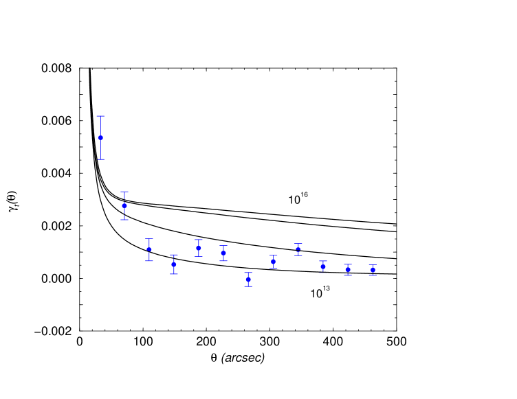
Figure 2.9: The SDSS galaxy-mass cross-correlation using galaxy-shear correlation function. The halo model predictions are shown here as a function of maximum mass for the dark matter halo used in the calculation: from top to bottom curves are for $10^{16},10^{15},10^{14}$ and 10¹³ M${}_{\sun}$. The data are from [Fischer et al.] (2000).

Our description for the galaxy power spectrum, see § 1.7, allows us to extend the discussion to also consider cross-correlation between galaxies and mass. Such a cross-power spectrum can be probed through the weak lensing shear-galaxy correlation function. Here, observations involve the mean tangential shear due to graviational lensing given by

$$\left<\gamma_{t}(\theta)\right>=-\frac{1}{2}\frac{d\bar{\kappa}(\theta)}{d{\rm ln}\theta}\,,$$ (2.40)

where $\bar{\kappa}(\theta)$ is the mean convergence within a circular radius of $\theta$ ([Squires & Kaiser] 1996). Since the shear is correlated with foreground galaxy positions, one essentially probe the galaxy-mass correlation such that

$$\bar{\kappa}(\theta)=\int drW^{\rm lens}(r)W^{\rm gal}(r)\int dkkP_{{\rm gal}\delta}(k)\frac{2J_{1}(kd_{A}\theta)}{kd_{A}\theta}$$ (2.41)

and

$$\left<\gamma(\theta)\right>=\int drW^{\rm lens}(r)W^{\rm gal}(r)\int dkkP_{{\rm gal}\delta}(k)J_{2}(kd_{A}\theta)\,.$$ (2.42)

Here, $W^{\rm lens}$ is the lensing windown function introduced in Eq. 2.2, while $W^{\rm gal}$ is the normalized redshift distribution of foreground galaxies. Note that, in general, $W^{\rm lens}$ involves the redshift distribution of background sources beyond the simple single source redshift assumption.

The tangential shear-foreground galaxy correlation has been measured in the Sloan survey by [Fischer et al.] (2000) and we compare these measurements with predictions in Fig. 2.9. The observed measurements from the Sloan survey come only for field galaxies, and thus, it is likely that the correlation function does not include any contributions from massive halos and rather from medium to small mass halos that contain one to few galaxies. Our predictions, where we see a lack of significant correlation at large angular distances with the inclusion of massive halos, are consistent with this observation. A more thorough study of the weak lensing shear-galaxy cross-correlation, under the halo model, is available in [Guzik & Seljak] (2000) and we refer the reader to this paper for further details.

2.5 Summary

We have presented an efficient method to calculate the non-Gaussian statistics of lensing convergence at the three point level based on a description of the underlying density field in terms of dark matter halos. The bispectrum contains all of the three point information, including the skewness. The prior attempts at calculating lensing bispectrum and skewness were limited by the accuracy of perturbative approximations and the dynamic range and sample variance of simulations.

Though the present technique provides a clear and an efficient method to calculate the statistics of the convergence field, it has its own shortcomings. Halos are not all spherical, which can to some extent affect the configuration dependence in moments higher than the two point level. Substructures due to mergers of halos can also introduce scatter. Though such effects unlikely to dominate our calculations, further work using numerical simulations will be necessary to determine to what extent present method can be used as a precise tool to study the higher order statistics associated with weak gravitational lensing.

The dark matter halo approach also allows one to study possible selection effects that may be present in weak lensing observations due to the presence or absence of rare massive halos in the small fields that are observed. We have shown that the weak lensing skewness is mostly due to the most massive and rarest dark matter halos in the universe. The effect of such halos is stronger at the three point level than the two point level. The absence of massive halos, with masses greater than $10^{14}$ M${}_{\sun}$, leads to a strong decrease in skewness, suggesting that a straightforward use of measured skewness values as a test of cosmological models may not be appropriate unless prior observations are available on the distribution of masses in observed lensing fields.

One can correct for such biases using the halo approach, however. To implement such a correction in practice, further work will be needed to calibrate the technique precisely against simulations across a wide range of cosmologies. Efficient techniques to correct for mass biases both in the lensing power spectrum and bispectrum will be needed. Alternatively, this technique can be used to search for generalized three point statistics that are more robust to sampling issues. Given the great potential to study the dark matter distribution through weak lensing, this issues merit further study.

Chapter 3 Weak Gravitational lensing Covariance

3.1 General Definitions

As discussed in the previous section, weak lensing probes the statistical properties of the shear field on the sky which is a weighted projection of the matter distribution along the line of sight to the source galaxies. As such, observables can be reexpressed as a scalar quantity, the convergence $\kappa$, on the sky.

The power spectrum and trispectrum of convergence are defined in the flat sky approximation in the usual way

$$\left<\kappa({\mathbf{l}}_{1})\kappa({\mathbf{l}}_{2})\right> = (2\pi)^{2}\delta_{\rm D}({\mathbf{l}}_{12})C_{l}^{\kappa}\,,$$

$$\left<\kappa({\mathbf{l}}_{1})\ldots\kappa({\mathbf{l}}_{4})\right>_{c} = (2\pi)^{2}\delta_{\rm D}({\mathbf{l}}_{1234})T^{\kappa}({\mathbf{l}}_{1},{\mathbf{l}}_{2},{\mathbf{l}}_{3},{\mathbf{l}}_{4})\,.$$ (3.1)

These are related to the density power spectrum and trispectrum by the projections ([Kaiser] 1992; [Scoccimarro et al.] 1999)

$$C^{\kappa}_{l} = \int dr\frac{W(r)^{2}}{d_{A}^{2}}P\left(\frac{l}{d_{A}};r\right)\,,$$ (3.2)

$$T^{\kappa} = \int dr\frac{W(r)^{4}}{d_{A}^{6}}T\left(\frac{{\mathbf{l}}_{1}}{d_{A}},\frac{{\mathbf{l}}_{2}}{d_{A}},\frac{{\mathbf{l}}_{3}}{d_{A}},\frac{{\mathbf{l}}_{4}}{d_{A}},;r\right)\,,$$ (3.3)

where $r$ is the comoving distance and $d_{A}$ is the angular diameter distance with the weight function defined in Eq. 2.3. For simplicity, we will assume $r_{s}=r(z_{s}=1)$.

For the purpose of this calculation, we assume that upcoming weak lensing convergence power spectrum will measure binned logarithmic band powers at several $l_{i}$’s in multipole space with bins of thickness $\delta l_{i}$.

$${\cal C}_{i}=\int_{{\rm s}i}{d^{2}l\over{A_{{\rm s}i}}}\frac{l^{2}}{2\pi}\kappa(\bf l)\kappa(-\bf l)\,,$$ (3.4)

where $A_{\rm s}(l_{i})=\int d^{2}l$ is the area of the two-dimensional shell in multipole and can be written as $A_{\rm s}(l_{i})=2\pi l_{i}\delta l_{i}+\pi(\delta l_{i})^{2}$.

We can now write the signal covariance matrix as

$$C_{ij} = {1\over A}\left[{(2\pi)^{2}\over A_{{\rm s}i}}2{\cal C}_{i}^{2}+T^{\kappa}_{ij}\right]\,,$$ (3.5)

$$T^{\kappa}_{ij} = \int{d^{2}l_{i}\over A_{{\rm s}i}}\int{d^{2}l_{j}\over A_{{\rm s}j}}{l_{i}^{2}l_{j}^{2}\over(2\pi)^{2}}T^{\kappa}({\mathbf{l}}_{i},-{\mathbf{l}}_{i},{\mathbf{l}}_{j},-{\mathbf{l}}_{j})\,,$$ (3.6)

where $A$ is the area of the survey in steradians. Again the first term is the Gaussian contribution to the sample variance and the second the non-Gaussian contribution. A realistic survey will also have shot noise variance due to the finite number of source galaxies in the survey. We will return to this point in the §3.3.

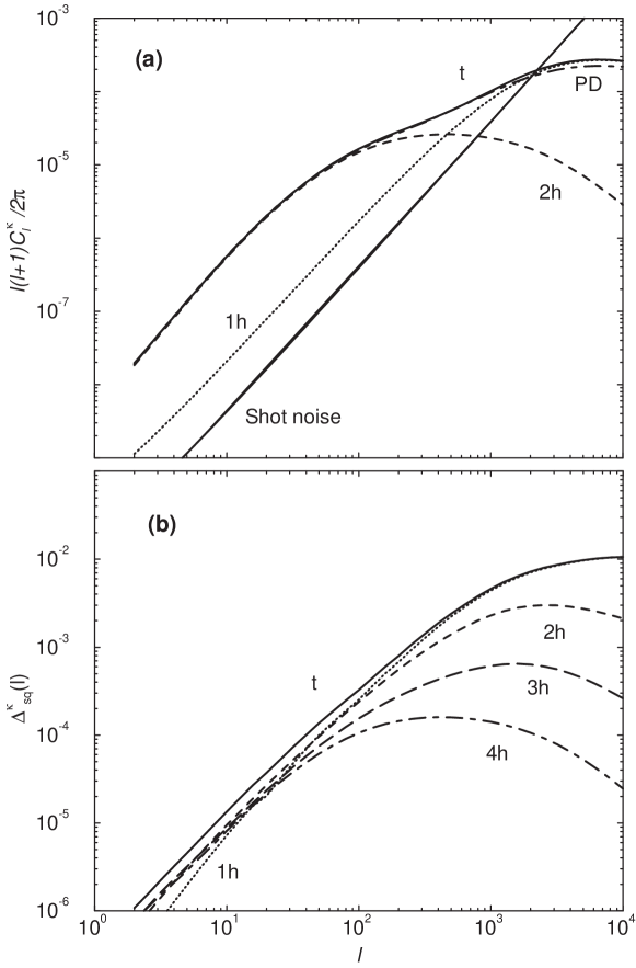
Figure 3.1: Weak lensing convergence (a) power spectrum and (b) trispectrum under the halo description. Also shown in (a) is the prediction from the PD nonlinear power spectrum fitting function. We have separated individual contributions under the halo approach and have assumed that all sources are at $z_{s}=1$. We have also shown the shot noise contribution to the power spectrum assuming a survey down to a limiting magnitude of R $\sim$ 25 with an intrinsic rms shear of 0.4 in each component.

3.2 Comparisons

Using the halo model, we can now calculate contributions to lensing convergence power spectrum and trispectrum. The power spectrum, shown in Fig. 3.1(a), shows the same behavior as the density field when compared with the PD results: a slight overprediction of power when $l\gtrsim 10^{3}$. This results through the distribution of the concentration-mass relation from simulations by [Bullock et al] (2000); In comparison to the previous chapter, we now include the full information on concentration from simulations to be complete instead of the fitting function for concentration which results in the recovery of PD non-linear power spectrum for dark matter. As shown in Fig. 3.1(a), the differences arising from variations in the concentration-mass relations are not likely to be observable given the shot noise from the finite number of galaxies at small scales.

In Fig 3.1(b), we show the scaled trispectrum

$$\Delta^{\kappa}_{\rm sq}(l)=\frac{l^{2}}{2\pi}T^{\kappa}({\bf l},-{\bf l},{\bf l}_{\perp},-{\bf l}_{\perp})^{1/3}\,.$$ (3.7)

where $l_{\perp}=l$ and ${\bf l}\cdot{\bf l}_{\perp}=0$. The projected lensing trispectrum again shows the same behavior as the density field trispectrum with similar conditions on ${\bf k}_{i}$’s.

We can now use this trispectrum to study the contributions to the covariance, which is what we are primarily concerned here. In Fig. 3.2a, we show the fractional error,

$${\Delta{\cal C}_{i}\over{\cal C}_{i}}\equiv{\sqrt{C_{ii}}\over{\cal C}_{i}}\,,$$ (3.8)

for bands $l_{i}$ given in Table 3.1 following the binning scheme used by [White & Hu] (1999) on $6^{\circ}\times 6^{\circ}$ fields.

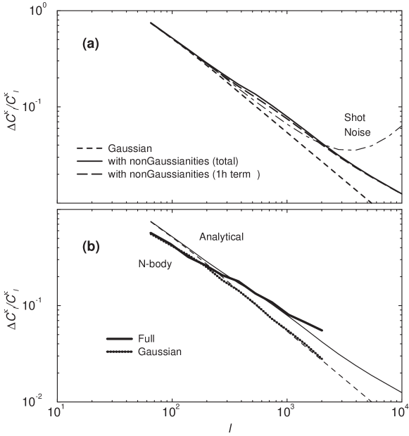
Figure 3.2: The fractional errors in the measurements of the convergence band powers. In (a), we show the fractional errors under the Gaussian approximation, the full halo description, the Gaussian plus single halo term, and the Gaussian plus shot noise term (see §3.3). As shown, the additional variance can be modeled with the single halo piece while shot noise generally becomes dominant before non-Gaussian effects become large. In (b), we compare the halo model with simulations from [White & Hu] (1999). The decrease in the variance at small $l$ in the simulations is due to the conversion of variance to covariance by the finite box size of the simulations.

The dashed line compares that with the Gaussian errors, involving the first term in the covariance (Eq. 3.6). At multipoles of a few hundred and greater, the non-Gaussian term begins to dominate the contributions. For this reason, the errors are well approximated by simply taking the Gaussian and single halo contributions.

In Fig. 3.2(b), we compare these results with those of the [White & Hu] (1999) simulations. The decrease in errors from the simulations at small $l$ reflects finite box effects that convert variance to covariance as the fundamental mode in the box becomes comparable to the bandwidth.

The correlation between the bands is given by

$$\hat{C}_{ij}\equiv\frac{C_{ij}}{\sqrt{C_{ii}C_{jj}}}\,.$$ (3.9)

In Table 3.1 we compare the halo predictions to the simulations by [White & Hu] (1999). The upper triangle here is the correlations under the halo approach, while the lower triangle shows the correlations found in numerical simulations. The correlations along individual columns increase (as one goes to large $l$’s or small angular scales) consistent with simulations. In Fig. 3.3, we show the correlation coefficients with (a) and without (b) the Gaussian contribution to the diagonal.

$\ell_{\rm bin}$	138	194	271	378	529	739	1031	1440	2012
138	1.00	0.08	0.10	0.11	0.12	0.12	0.12	0.11	0.11
194	(0.31)	1.00	0.14	0.17	0.18	0.18	0.17	0.16	0.15
271	(0.21)	(0.26)	1.00	0.24	0.25	0.25	0.24	0.22	0.21
378	(0.09)	(0.24)	(0.38)	1.00	0.33	0.33	0.32	0.30	0.28
529	(0.14)	(0.28)	(0.33)	(0.45)	1.00	0.42	0.40	0.37	0.35
739	(0.16)	(0.17)	(0.34)	(0.38)	(0.50)	1.00	0.48	0.45	0.42
1031	(0.18)	(0.15)	(0.27)	(0.33)	(0.48)	(0.54)	1.00	0.52	0.48
1440	(0.15)	(0.19)	(0.19)	(0.32)	(0.36)	(0.53)	(0.57)	1.00	0.54
2012	(0.22)	(0.16)	(0.32)	(0.27)	(0.46)	(0.50)	(0.61)	(0.65)	1.00

Table 3.1: Covariance of the binned power spectrum when sources are at a redshift of 1. Upper triangle displays the covariance found under the halo model. Lower triangle (parenthetical numbers) displays the covariance found in numerical simulations by [White & Hu] (1999). To be consistent with these simulations, we use the same binning scheme as the one used there.

We show in Fig. 3.3(a) the behavior of the correlation coefficient between a fixed $l_{j}$ as a function of $l_{i}$. When $l_{i}=l_{j}$ the coefficient is 1 by definition. Due to the presence of the dominant Gaussian contribution at $l_{i}=l_{j}$, the coefficient has an apparent discontinuity between $l_{i}=l_{j}$ and $l_{i}=l_{j-1}$ that decreases as $l_{j}$ increases and non-Gaussian effects dominate.

To better understand this behavior it is useful to isolate the purely non-Gaussian correlation coefficient

$$\hat{C}^{\rm NG}_{ij}=\frac{T_{ij}}{\sqrt{T_{ii}T_{ij}}}\,.$$ (3.10)

As shown in Fig. 3.3(b), the coefficient remains constant for $l_{i}\ll l_{j}$ and smoothly increases to unity across a transition scale that is related to where the single halo terms starts to contribute. A comparison of Fig. 3.3(b) and 2.1(b), shows that this transition happens around $l$ of few hundred to 1000. Once the power spectrum is dominated by correlations in single halos, the fixed profile of the halos will correlate the power in all the modes. The multiple halo terms on the other hand correlate linear and non-linear scales but at a level that is generally negligible compared with the Gaussian variance.

The behavior seen in the halo based covariance, however, is not present when the covariance is calculated with hierarchical arguments for the trispectrum (see, [Scoccimarro et al.] 1999). With hierarchical arguments, which are by construction only valid in the deeply nonlinear regime, one predicts correlations which are, in general, constant across all scales and shows no decrease in correlations between very small and very large scales. Such hierarchical models also violate the Schwarz inequality with correlations greater than 1 between large and small scales (e.g., [Scoccimarro et al.] 1999; [Hamilton] 2000). The halo model, however, shows a decrease in correlations similar to numerical simulations suggesting that the halo model, at least qualitatively, provides a better approach to studying non-Gaussian correlations in the translinear regime.

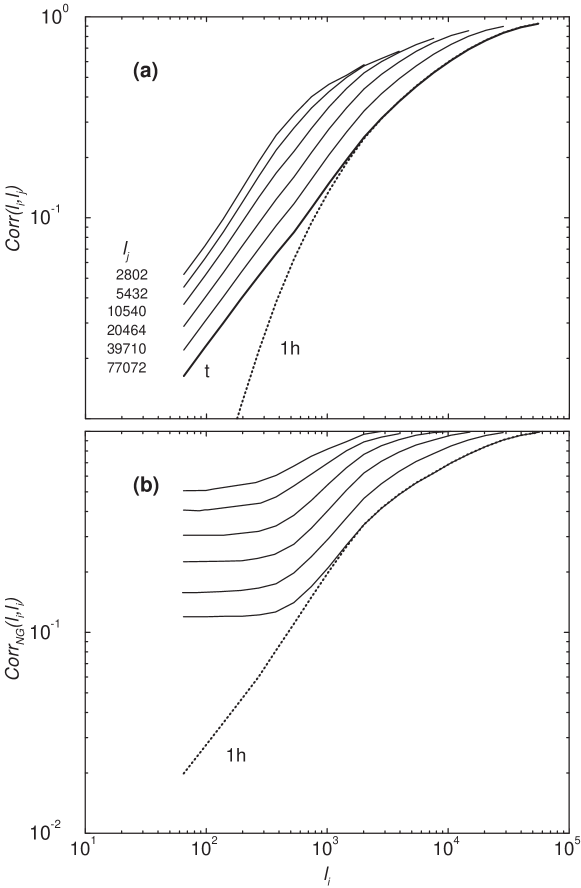
Figure 3.3: (a) The correlation coefficient, $\hat{C}_{ij}$ as a function of the multipole $l_{i}$ with $l_{j}$ as shown in the figure. We show the correlations calculated with the full halo model and also with only the single halo term for $l_{j}=77072$. In (b), we show the non-Gaussian correlation coefficient $\hat{C}_{ij}^{\rm NG}$, which only involves the trispectrum (see, Eq. 3.10). The transition to full correlation is due to the domination of the single halo contribution.

3.3 Effect on Parameter Estimation

Modeling or measuring the covariance matrix of the power spectrum estimates will be essential for interpreting observational results. In the absence of many fields where the covariance can be estimated directly from the data, the halo model provides a useful, albeit model dependent, quantification of the covariance. As a practical approach one could imagine taking the variances estimated from the survey under a Gaussian approximation, but which accounts for uneven sampling and edge effects ([Hu & White] 2000), and scaling it up by the non-Gaussian to Gaussian variance ratio of the halo model along with inclusion of the band power correlations. Additionally, it is in principle possible to use the expected correlations from the halo model to decorrelate individual band power measurements, similar to studies involving CMB temperature anisotropy and galaxy power spectra (e.g., [Hamilton] 1997; [Hamilton & Tegmark] 2000).

We can estimate the resulting effects on cosmological parameter estimation with an analogous procedure on the Fisher matrix. In [Hu & Tegmark] (1999), the potential of wide-field lensing surveys to measure cosmological parameters was investigated using the Gaussian approximation of a diagonal covariance and Fisher matrix techniques. The Fisher matrix is simply a projection of the covariance matrix onto the basis of cosmological parameters $p_{i}$

$${\bf F}_{\alpha\beta}=\sum_{ij}{\partial{\cal C}_{i}\over\partial p_{\alpha}}(C_{\rm tot}^{-1})_{ij}{\partial{\cal C}_{j}\over\partial p_{\beta}}\,,$$ (3.11)

where the total covariance includes both the signal and noise covariance. Under the approximation of Gaussian shot noise, this reduces to replacing $C^{\kappa}_{l}\rightarrow C^{\kappa}_{l}+C^{\rm SN}_{l}$ in the expressions leading up to the covariance Eq. 3.6. The shot noise power spectrum is given by

$$C^{\rm SN}_{l}=\frac{\langle\gamma_{\rm int}^{2}\rangle}{\bar{n}}\,,$$ (3.12)

where $\langle\gamma_{\rm int}\rangle^{1/2}\sim 0.4$ is the rms noise per component introduced by intrinsic ellipticities and measurement errors and $\bar{n}\sim 6.6\times 10^{8}$ sr^-1 is the surface number density of background source galaxies. The numerical values here are appropriate for surveys that reach a limiting magnitude in $R\sim 25$ (e.g., [Smail et al] 1995).

Under the approximation that there are a sufficient number of modes in the band powers that the distribution of power spectrum estimates is approximately Gaussian, the Fisher matrix quantifies the best possible errors on cosmological parameters that can be achieved by a given survey. In particular $F^{-1}$ is the optimal covariance matrix of the parameters and $(F^{-1})_{ii}^{1/2}$ is the optimal error on the $i$th parameter. Implicit in this approximation of the Fisher matrix is the neglect of information from the cosmological parameter dependence of the covariance matrix of the band powers themselves. Since the covariance is much less than the mean power, we expect this information content to be small.

In order to estimate the effect of non-Gaussianities on the cosmological parameters, we calculate the Fisher matrix elements using our fiducial $\Lambda$CDM cosmological model and define the dark matter density field, today, as

$$\Delta^{2}(k)=A^{2}\left(\frac{k}{H_{0}}\right)^{n_{s}+3}T^{2}(k)\,.$$ (3.13)

Here, $A$ is the amplitude of the present day density fluctuations and $n_{s}$ is the tilt at the Hubble scale. The density power spectrum is evolved to higher redshifts using the growth function $G(z)$ ([Peebles] 1980) and the transfer function $T(k)$ is calculated using the fitting functions from [Eisenstein & Hu] (1999). Since we are only interested in the relative effect of non-Gaussianities, we restrict ourselves to a small subset of the cosmological parameters considered by [Hu & Tegmark] (1999) and assume a full sky survey with $f_{\rm sky}=1$.

$p_{i}$	$\Omega_{\Lambda}$	$\ln$ A	$\Omega_{K}$	$n_{s}$	$\Omega_{m}h^{2}$
$\Omega_{\Lambda}$	1.57	-5.96	-1.39	4.41	-1.76
$\ln$ A		25.89	5.83	-17.34	6.74
$\Omega_{K}$			1.41	-3.81	1.43
$n_{s}$				14.01	-6.03
$\Omega_{m}h^{2}$					2.67

$p_{i}$	$\Omega_{\Lambda}$	$\ln$ A	$\Omega_{K}$	$n_{s}$	$\Omega_{m}h^{2}$
$\Omega_{\Lambda}$	2.03	-7.84	-1.82	5.76	-2.30
$\ln$ A		33.92	7.65	-22.79	8.91
$\Omega_{K}$			1.78	-5.01	1.95
$n_{s}$				18.43	-7.85
$\Omega_{m}h^{2}$					3.44

Table 3.2: Inverse Fisher matrix under the Gaussian assumption (top) and the halo model (bottom). The error on an individual parameter is the square root of the diagonal element of the Fisher matrix for the parameter while off-diagonal entries of the inverse Fisher matrix shows correlations, and, thus, degeneracies, between parameters. We have assumed a full sky survey ($f_{\rm sky}=1$) with parameters as described in § 3.3.

In Table 3.2, we show the inverse Fisher matrices determined under the Gaussian and non-Gaussian covariances, respectively. For the purpose of this calculation, we adopt the binning scheme as shown in Table 3.1, following [White & Hu] (1999). The Gaussian errors are computed using the same scheme by setting $T^{\kappa}=0$. As shown in Table 3.2, the inclusion of non-Gaussianities lead to an increase in the inverse Fisher matrix elements. We compare the errors on individual parameters, mainly $(F^{-1})_{ii}^{1/2}$, between the Gaussian and non-Gaussian assumptions in Table 3.3. The errors increase typically by $\sim 15$%. Note also that band power correlations do not necessarily increase cosmological parameter errors. Correlations induced by non-linear gravity introduce larger errors in the overall amplitude of the power spectrum measurements but have a much smaller effect on those parameters controlling the shape of the spectrum.

For a survey of this assumed depth, the shot noise power becomes the dominant error before the non-Gaussian signal effects dominate over the Gaussian ones. For a deeper survey with better imaging, such as the one planned with Large-aperture Synoptic Survey Telescope (LSST; [Tyson & Angel] 2000), the effect of shot noise decreases and non-Gaussianity is potentially more important. However, the non-Gaussianity itself also decreases with survey depth, and as we now discuss, in terms of the effect of non-Gaussianities, deeper surveys should be preferred over the shallow ones.

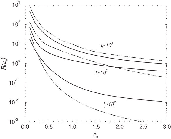
Figure 3.4: The ratio of non-Gaussian to Gaussian contributions, $R$, as a function of source redshift ($z_{s}$). The solid lines are through the exact calculation (Eq. 3.15) while the dotted lines are using the approximation given in Eq. 3.16. Here, we show the ratio $R$ for three multipoles corresponding to large, medium and small angular scales. The multipole binning is kept constant such that $\delta l\sim l$. Decreasing this bin size will linearly decrease the value of $R$.

3.4 Scaling Relations

To better understand how the non-Gaussian contribution scale with our assumptions, we consider the ratio of non-Gaussian variance to the Gaussian variance

$$\frac{C_{ii}}{C_{ii}^{\rm G}}=1+R\,,$$ (3.14)

with

$$R\equiv\frac{A_{si}T_{ii}^{\kappa}}{(2\pi)^{2}2C_{i}^{2}}\,.$$ (3.15)

Under the assumption that contributions to lensing convergence can be written through an effective distance $r_{\star}$, at half the angular diameter distance to background sources, and a width $\Delta r$ for the lensing window function, the ratio of lensing convergence trispectrum and power spectrum contribution to the variance can be further simplified to

$$R\sim\frac{A_{si}}{(2\pi)^{2}V_{\rm eff}}\frac{\bar{T}(r_{\star})}{2\bar{P}^{2}(r_{\star})}\,.$$ (3.16)

Since the lensing window function peaks at $r_{\star}$, we have replaced the integral over the window function of the density field trispectrum and power spectrum by its value at the peak. This ratio shows how the relative contribution from non-Gaussianities scale with survey parameters: (a) increasing the bin size, through $A_{si}$ ($\propto\delta l$), leads to an increase in the non-Gaussian contribution linearly, (b) increasing the source redshift, through the effective volume of lenses in the survey ($V_{\rm eff}\sim r_{\star}^{2}\Delta r$), decreases the non-Gaussian contribution, while (c) the growth of the density field trispectrum and power spectrum, through the ratio $\bar{T}/\bar{P}^{2}$, decreases the contribution as one moves to a higher redshift. The volume factor quantifies the number of foreground halos in the survey that effectively act as gravitational lenses for background sources; as the number of such halos is increased, the non-Gaussianities are reduced by the central limit theorem.

In Fig. 3.4, we summarize our results as a function of source redshift with $l_{i}\sim 10^{2},10^{3}$ and 10⁴ and setting the bin width such that $A_{s}(l_{i})\sim l_{i}^{2}$, or $\delta l\sim l$. As shown, increasing the source redshift leads to a decrease in the non-Gaussian contribution to the variance. The prediction based on the simplifications in Eq. 3.16 tend to overestimate the non-Gaussianity at lower redshifts while underestimates it at higher redshifts, though the exact transition depends on the angular scale of interest; this behavior can be understood due to the fact that we do not consider the full lensing window function but only the contributions at an effective redshift, midway between the observer and sources.

In order to determine whether its the increase in volume or the decrease in the growth of structures that lead to a decrease in the relative importance of non-Gaussianities as one moves to a higher source redshift, we calculated the non-Gaussian to Gaussian variance ratio under the halo model for several source redshifts and survey volumes. Up to source redshifts $\sim$ 1.5, the increase in volume decreases the non-Gaussian contribution significantly. When surveys are sensitive to sources at redshifts beyond 1.5, the increase in volume becomes less significant and the decrease in the growth of structures begin to be important in decreasing the non-Gaussian contribution. Since, in the deeply non-linear regime, $\bar{T}/\bar{P}^{2}$ scales with redshift as the cube of the growth factor, this behavior is consistent with the overall redshift scaling of the volume and growth.

The importance of the non-Gaussianity to the variance also scales linearly with bin width. As one increases the bin width the covariance induced by the non-Gaussianity manifests itself as increased variance relative to the Gaussian case. The normalization of $R$ is therefore somewhat arbitrary in that it depends on the binning scheme, i.e. $R\ll 1$ does not necessarily mean non-Gaussianity can be entirely neglected when summing over all the bins. The scaling with redshift and the overall scaling of the variance with the survey area $A$ is not. One way to get around the increased non-Gaussianity associated with shallow surveys, is to have it sample a wide patch of sky since $C_{ii}\propto(1+R)/A$. This relation tells us the trade off between designing an survey to go wide instead of deep. One should bear in mind though that not only will shallow surveys have decreasing number densities of source galaxies and hence increasing shot noise, they will also suffer more from the decreasing amplitude of the signal itself and the increasing import ance of systematic effects, including the intrinsic correlations of galaxy shapes (e.g., [Catelan et al] 2000; [Croft & Metzler] 2000; [Heavens et al.] 2000). These problems tilt the balance more towards deep but narrow surveys than the naive statistical scaling would suggest.

	$\Omega_{\Lambda}$	$\ln$ A	$\Omega_{k}$	$n_{s}$	$\Omega_{m}h^{2}$
Gaussian	0.039	0.160	0.037	0.118	0.051
Full	0.045	0.184	0.042	0.135	0.058
Increase (%)	15.3	15	13.5	14.4	13.7

Table 3.3: Parameter errors, $(F^{-1})_{ii}^{1/2}$, under the Gaussian assumption (top) and the halo model (bottom) and following the inverse-Fisher matrices in Table 3. We have assumed a full sky survey ($f_{\rm sky}=1$) with parameters as described in § 3.3.

3.5 Conclusions

Weak gravitational lensing due to large scale structure provides important information on the evolution of clustering and angular diameter distances and therefore, cosmological parameters. This information complements what can be learned from cosmic microwave background anisotropy observations. The tremendous progress on the observational front warrants detailed studies of the statistical properties of the lensing observables and their use in constraining cosmological models.

The non-linear growth of large-scale structure induces high order correlations in the derived shear and convergence fields. In this work, we have studied the four point correlations in the fields. Four point statistics are special in that they quantify the errors in the determination of the two point statistics. To interpret future lensing measurements on the power spectrum, it will be essential to have an accurate assessment of the correlation between the measurements.

Using the halo model for clustering, we have provided a semi-analytical method to calculate the four point function of the lensing convergence as well as the dark matter density field. We have tested this model against numerical $N$-body simulations of the power spectrum covariance in both the density and convergence fields and obtained good agreement. As such, this method provides a practical means of estimating the error matrix from future surveys in the absence of sufficiently large fields where it may be estimated directly from the data or large suites of $N$-body

simulations where it can be quantified in a given model context. Eventually a test of whether the covariance matrix estimated from the data and the theory agree may even provide further cosmological constraints. This method may also be used to study other aspects of the four point function in lensing and any field whose relation to the dark matter density field can be modeled. Given the approximate nature of these approximations, each potential use must be tested against simulations. Nonetheless, the halo model provides the most intuitive and extensible means to study non-Gaussianity in the cosmological context currently known.

Chapter 4 Thermal Sunyaev-Zel’dovich Effect

4.1 Introduction

In recent years, increasing attention has been given to the physical properties of the intergalactic warm and hot plasma gas distribution associated with large scale structure and the possibility of its detection (e.g., [Cen & Ostriker] 1999). It is now widely believed that at least $\sim$ 50% of the present day baryons, when compared to the total baryon density through big bang nucleosynthesis, are present in this warm gas distribution and have remained undetected given its nature (e.g., [Fukugita et al] 1998). Currently proposed methods for the detection of this gas with include observations of the thermal diffuse X-ray emission (e.g., [Pierre et al.] 2000), associated X-ray and UV absorption and emission lines (e.g., [Tripp et al.] 2000) and resulting Sunyaev-Zel’dovich (SZ; [Sunyaev & Zel’dovich] 1980) effect (e.g., [Cooray et al.] 2000a).

The SZ effect arises from the inverse-Compton scattering of CMB photons by hot electrons along the line of sight. This effect has now been directly imaged towards massive galaxy clusters (e.g., [Carlstrom et al.] 1996; [Jones et al] 1993), where the temperature of the scattering medium can reach as high as 10 keV, producing temperature changes in the CMB of order 1 mK at Rayleigh-Jeans wavelengths. Previous analytical predictions of the resulting SZ effect due to large scale structure have been based on either through a Press-Schechter (PS; [Press & Schechter] 1974) description of the contributing galaxy clusters (e.g., [Cole & Kaiser] 1988; [Komatsu & Kitayama] 1999) or using a biased description of the pressure power spectrum with respect to the dark matter density field (e.g., [Cooray et al.] 2000a). Numerical simulations (e.g., [da Silva et al.] 1999; [Refregier et al.] 1999; [Seljak et al.] 2000; [Springel et al.] 2000) are beginning to improve some of these analytical predictions, but are still limited to handful of simulations with limited dynamical range and resolution. Therefore, it is important that one consider improving analytical models of the large scale structure SZ effect, and provide predictions which can be easily tested through simulations.

Our present study on the large scale baryon pressure and the resulting SZ effect is timely for two main reasons. First, the improvements in hydrodynamical simulations now allow detailed predictions on the statistics of pressure power spectrum and resulting SZ effect (e.g., [Springel et al.] 2000; [Refregier & Teyssier] 2001). The numerical studies are easily extendable to higher order correlations through models such as the halo based one advocated here. Here, we extend previous analytical and numerical studies by considering the full power spectrum, bispectrum, and trispectrum of pressure fluctuations. The pressure correlations contain all necessary information on the large scale distribution of temperature weighted baryons, whereas, the thermal SZ angular power spectrum is only a redshift projected measurement of the pressure power spectrum. This can be compared to weak gravitational lensing, where lensing is a direct probe of the projected dark matter density distribution. The bispectrum of pressure fluctuations, and SZ bispectrum, contains all the information present at the three-point level, whereas conventional statistics, such as skewness, do not. An useful advantage of using three-dimensional statistics, such as the pressure power spectrum, is that they can directly compared to numerical simulations, while only two-dimensional statistics, such as the projected pressure power spectrum along the line of sight, basically the SZ power spectrum, can only be observed. Our approach here is to consider both such that our calculations can eventually be compared to both simulations and observations.

The calculation of pressure power spectrum and higher order correlations requires detailed knowledge on the baryon distribution, which can eventually be obtained numerically through hydrodynamical simulations. Here, we provide an analytical technique to obtain the pressure power spectrum, bispectrum and trispectrum by extending the dark matter halo approach. The baryons are assumed to be in hydrostatic equilibrium with respect to dark matter distribution, which is a valid assumption, at least for the high mass halos that have been observed with X-ray instruments, given the existence of regularity relations between cluster baryon and dark matter physical properties (e.g., [Mohr & Evrard] 1997). We take a description of the temperature structure of electrons involving the virial temperature. When estimating astrophysical parameters from the SZ effect, we will consider an an additional source of non-gravitational energy, independent of mass and redshift. The latter consideration allows the possibility for a secondary source of energy for baryons, such as due to preheating through stellar formation and feedback processes. Numerical simulations (e.g., [Cen & Ostriker] 1999; [Pen] 1999), as well observations (e.g., [David et al.] 1995; [Renzini] 1997), suggest the existence of such an energy source.

The second reason why this study is timely is that the progress in the experimental front strongly suggests possibilities for detailed observational studies of the SZ power spectrum and higher order correlations. Given that the SZ effect also bears a spectral signature that differs from other temperature fluctuations, SZ contribution can be separated in upcoming multifrequency CMB data. As discussed in detail in [Cooray et al.] (2000a), a multi-frequency approach can easily be applied to current Boomerang ([de Bernardis et al.] 2000), and upcoming MAP and Planck surveyor missions. At small angular scales, though a wide-field SZ image, is yet to be produced, several experiments are now working towards this goal. These experimental attempts include the interferometric survey by [Carlstrom et al.] (1996) at the combined BIMA/OVRO array (CARMA), the MINT interferometer (Lyman Page, private communication), and the BOLOCAM array on the Caltech Submillimeter Observatory (Andrew Lange, private communication).

In the present Chapter, we discuss the SZ effect and address what astrophysical properties can be deduced with a measurement of the SZ power spectrum. For this, we require detailed knowledge on the covariance of the SZ power spectrum beyond the simple Gaussian assumptions for the variance. Given that the SZ effect probes the projected pressure distribution in the local universe, its statistical properties reflect those of pressure. As discussed in detail in [Cooray] (2000), the statistics of large scale structure pressure is highly non-Gaussian due to the associated non-linearities. We have previously shown that the SZ effect has a significant skewness associated with it, primarily given that the large scale pressure power spectrum is associated with massive halos, which are rare and discrete. The same non-Gaussianities also induce a four-point correlation function in pressure, which in return, can be used to study the correlations in the pressure power spectrum due to resulting non-Gaussian covariance. This is is analogous to the dark matter covariance correlations discussed in [Meiksin & White] (1999) and [Scoccimarro et al.] (1999), using numerical simulations, and in [Cooray & Hu] (2001b) using the halo model. The pressure trispectrum is also of interest since it determines the covariance of the thermal SZ power spectrum measurements. Again, this is analogous to the covariance we recently discussed for weak gravitational lensing ([Cooray & Hu] 2001b) resulting from the trispectrum of dark matter due to non-linear clustering at low redshifts and the covariance discussed in [Eisenstein & Zaldarriaga] (2001) for the APM galaxy power spectrum.

In order to calculate the covariance associated with SZ power spectrum measurements, we extend the semi-analytical model presented in [Cooray] (2000) and calculate the pressure trispectrum. Here, we show that the SZ effect is highly non-Gaussian at all scales of interest and that these non-Gaussianities correlate the SZ power spectrum measurements significantly. The full covariance matrix now allows us to quantify the astrophysical abilities of SZ measurements as a probe of gas and its temperature properties. Previous to this study, we were unable to perform a detailed calculation on how well SZ effect probe gas and temperature properties due to the unknown covariance associated with the effect. We also briefly discuss some aspects of the clustering of SZ halos and suggest a useful way to obtain an average value of halo mass, as a function of redshift, through the correlation function and bias.

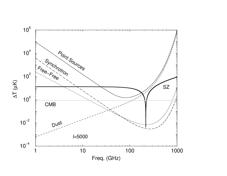
Figure 4.1: Frequency dependence of the SZ effect at a multipole of $l\sim 5000$. Here, we show the absolute value of temperature relative to the thermal CMB spectrum. For comparison, we also show the temperature fluctuations due to point sources (both radio at low frequencies and fra-infrared sources at high frequencies; solid line), galactic synchrotron (long dashed line), galactic free-free (dotted line) and galactic dust (short dashed line). At small angular scales, frequencies around 50 to 100 GHz is ideal for a SZ experiment.

4.2 Frequency Separation

The main obstacle for the detection of the SZ effect from large-scale structure for angular scales above a few arcminutes is the CMB itself. Here the primary anisotropies dominate the SZ effect for frequencies near and below the peak in the CMB spectrum (see Fig. 4.2). Fortunately, the known frequency dependence and statistical properties of primary anisotropies allows for extremely effective subtraction of their contribution (e.g., [Hobson et al] 1998; [Bouchet & Gispert] 1999). In particular, primary anisotropies obey Gaussian statistics and follow the blackbody spectrum precisely.

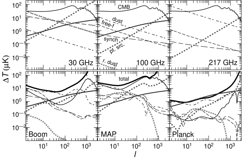
Figure 4.2: Top: foreground contributions to temperature anisotropies $(\Delta T/T)^{2}=l(l+1)C_{l}/2\pi$ from the various foregrounds (dust, free-free, synchrotron, radio and infrared point sources, and rotating dust) at three fiducial frequencies as labeled. The SZ signal (solid, unlabeled) is estimated with a simplified biased tracer model (see, [Cooray et al.] 2000a). Bottom: residual foregrounds after multifrequency subtraction for Boomerang, MAP and Planck. The total includes detector noise and residual CMB.

Perhaps more worrying are the galactic and extragalactic foregrounds, some of which are expected to to be at least comparable to the SZ signal in each frequency band. These foregrounds typically have spatial and/or temporal variations in their frequency dependence leading to imperfect correlations between their contributions in different frequency bands. We attempt here to provide as realistic an estimate as possible of the prospects for CMB and foreground removal, given our incomplete understanding of the foregrounds. In Fig. 4.1, we summarize our knowledge on the frequency dependence of the SZ, CMB and other foreground contaminants. Here, we consider a small angular scale experiments and all effects are scaled relative to the thermal CMB spectrum. Other than CMB, the only well known spectral dependence in this plot is the SZ effect. To avoid complications in plotting, we only show the absolute value of temperature here, but, it should be understood that the SZ effect produces a decrement below the null frequency ($\sim$ 217 GHz) and an increment thereafter.

Experiment	$\nu$	FWHM	$10^{6}\Delta T/T$
Boomerang	90	20	7.4
	150	12	5.7
	240	12	10
	400	12	80
MAP	22	56	4.1
	30	41	5.7
	40	28	8.2
	60	21	11.0
	90	13	18.3
Planck	30	33	1.6
	44	23	2.4
	70	14	3.6
	100	10	4.3
	100	10.7	1.7
	143	8.0	2.0
	217	5.5	4.3
	353	5.0	14.4
	545	5.0	147
	857	5.0	6670

Table 4.1: Specifications used for Boomerang, MAP and Planck. Full width at half maxima (FWHM) of the beams are in arcminutes and should be converted to radians for the noise formula. Boomerang covers a fraction $\sim$ 2.6% of the sky, while we assume a usable fraction of 65% for MAP and Planck.

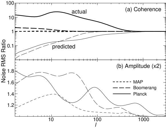
Figure 4.3: Dependence of the residual noise rms on foreground assumptions expressed as a ratio to the fiducial model of Fig. 4.2. (a) Falsely assuming the foregrounds have perfect frequency coherence not only underpredicts the residual noise by a substantial factor but also leads to substantially more actual residual noise. (b) Multiplying the foreground amplitudes by 2 (power by 4) produces less than a factor of 2 increase in the residual noise.

4.2.1 Foreground Model and Removal

We use the “MID” foreground model of [Tegmark et al.] (1999) and adapt the subtraction techniques found there for the purpose of extracting the SZ signal. The assumed level of the foreground signal in the power spectrum for three fiducial frequencies is shown in Fig. 4.2.

The foreground model is defined in terms of the covariance between the multipole moments at different frequency bands

$$\left<a_{l^{\prime}m^{\prime}}^{{\rm f}*}(\nu^{\prime})a_{lm}^{{\rm f}}(\nu)\right>=C_{l}^{{\rm f}}(\nu^{\prime},\nu)\delta_{ll^{\prime}}\delta_{mm^{\prime}}\,,$$ (4.1)

in thermodynamic temperature units as set by the CMB blackbody. In this section, we will speak of the primary anisotropies and detector noise simply as other foregrounds with very special properties:

$$C_{l}^{\rm CMB}(\nu^{\prime},\nu) = C_{l}\,,$$

$$C_{l}^{\rm noise}(\nu^{\prime},\nu) = 8\ln 2\theta(\nu)^{2}e^{\theta^{2}(\nu)l(l+1)}\left({\Delta T\over T}\right)^{2}\Big{|}_{\rm noise}\delta_{\nu,\nu^{\prime}}\,.$$

The FWHM$=\sqrt{8\ln 2}\theta$ and noise specifications of the Boomerang, MAP and Planck frequency channels are given in Tab. 1. True foregrounds generally fall in between these extremes of perfect and no frequency correlation.

The difference between extracting the SZ signal and the primary signal is simply that one performs the subtraction referenced to the SZ frequency dependence

$$s(\nu)=2-{x\over 2}\coth{x\over 2}\,,$$ (4.3)

where $x=h\nu/kT_{\rm cmb}\approx\nu/56.8$GHz. Note that in the RJ limit $s(\nu)\rightarrow 1$ such that

$$C_{l}^{\rm SZ}(\nu,\nu^{\prime})=s(\nu)s(\nu^{\prime})C_{l}^{\rm SZ}$$ (4.4)

where $C_{l}^{\rm SZ}$ is the SZ power spectrum in the RJ limit.

Consider an arbitrary linear combination of the channels,

$$b=\sum_{\nu_{i}}{1\over s(\nu_{i})}w(\nu_{i})a(\nu_{i})\,,$$ (4.5)

where we will normalize the sum of the weights to unity $\sum w(\nu_{i})=1$ to obtain an unbiased estimator of the RJ multipoles. Since the subtraction is done multipole by multipole, we have temporarily suppressed the multipole index. The covariance of this quantity is

$$\left<b^{2}\right>=C^{{\rm SZ}}[\sum_{\nu_{i}}w(\nu_{i})]^{2}+\sum_{\nu_{i},\nu_{j}}w(\nu_{i})w(\nu_{j})\tilde{C}(\nu_{i},\nu_{j})\,,$$ (4.6)

where the scaled foreground covariance matrix is

$$\tilde{C}(\nu_{i},\nu_{j})\equiv\sum_{{\rm f}}\tilde{C}^{\rm f}(\nu_{i},\nu_{j}) = \sum_{{\rm f}}{C^{\rm f}(\nu_{i},\nu_{j})\over s(\nu_{i})s(\nu_{j})}\,.$$ (4.7)

Minimizing the variance contributed by the foregrounds subject to the constraint that the SZ estimation be unbiased, we obtain

$$\sum_{\nu_{i}}w(\nu_{j}){\tilde{C}(\nu_{i},\nu_{j})}={\rm const.}\,$$ (4.8)

whose solution is ${\bf w}\propto\tilde{\bf C}^{-1}{\bf e}$, where $e(\nu_{i})=1$. The constant of proportionality is fixed by the condition $\sum w(\nu_{i})=1$, i.e.

$$w(\nu_{i})={\sum_{\nu_{j}}{\tilde{C}}^{-1}(\nu_{i},\nu_{j})\over\sum_{\nu_{k},\nu_{j}}{\tilde{C}}^{-1}(\nu_{k},\nu_{j})}\,.$$ (4.9)

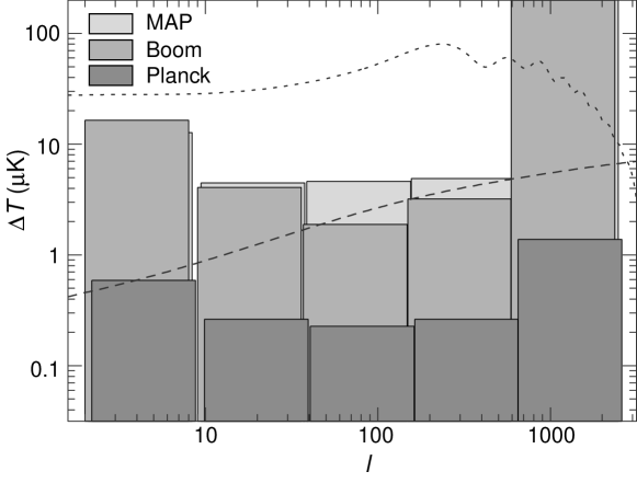
Figure 4.4: Detection thresholds for the SZ effect. Error boxes represent the 1-$\sigma$ rms residual noise in multipole bands and can be interpreted as the detection threshold. Also shown (dotted) is the level of the primary anisotropies that have been subtracted with the technique and the signal (dashed) expected in the simplified model of [Cooray et al.] (2000a).

4.2.2 Detection Threshold

The residual noise variance from each foreground component is then

$$N_{l}^{\rm f}=\sum_{\nu_{i},\nu_{j}}w_{l}(\nu_{i})w_{l}(\nu_{j})\tilde{C}_{l}^{\rm f}(\nu_{i},\nu_{j})\,.$$ (4.10)

with the total

$$N_{l}=\sum_{{\rm f}}N_{l}^{\rm f}\,,$$ (4.11)

where we have restored the multipole index.

Note that the residual noise in the map is independent of assumptions about the SZ signal including whether it is Gaussian or not. However if the foregrounds themselves are non-Gaussian, then this technique only minimizes the variance and may not be optimal for recovery of non-Gaussian features in the SZ map itself. [Bouchet et al] (1995) have shown that similar techniques are quite effective even when confronted with non-Gaussian foregrounds. This is a potential caveat especially for cases in which the residual noise is not dominated by the primary anisotropies or detector noise.

The residual noise sets the detection threshold for the SZ effect for a given experiment. In Fig. 4.2, we show the rms of the residual noise after foreground subtraction for the Boomerang, MAP and Planck experiments assuming the “MID” foreground model from [Tegmark et al.] (1999). With the Boomerang and Planck channels, elimination of the primary anisotropies is excellent up to the beam scale where detector noise dominates. As expected, the MAP channels, which are all on the RJ side of the spectrum, do not allow good elimination of the primary anisotropies.

It is important not to assume that the foregrounds are perfectly correlated in frequency, which is the usual assumption in the literature (e.g., [Hobson et al] 1998). There are two types of errors incurred by doing so. The first is that one underpredicts the amount of residual noise in the SZ map (see Fig. 4.3). The second is that if one calculates the optimal weights in Eq. 4.9 based on this assumption the actual residual noise increases. For Planck it can actually increase the noise beyond the level in which it appears in the $100$GHz maps with no foreground subtraction at all. The reason is that the cleaning algorithm then erroneously uses the contaminated high and low frequency channels to subtract out the small foreground contamination in the central channels. In Planck, the difference between the predicted and actual rms noise from falsely assuming perfect frequency coherence can be more than two orders of magnitude.

For Boomerang and Planck, the largest residual noise component, aside from detector noise, is dust emission and is sufficiently large that one might worry that current uncertainties in our knowledge of the foreground model may affect the implications for the detection of the SZ effect. It is therefore important to explore variations on our fiducial foreground model.

Multiplying the foreground rms amplitudes uniformly by a factor of 2 (and hence the power by a factor of 4), produces less than a factor of 2 increase in the residual noise rms as shown in Fig. 4.3. Likewise, as discussed in [Tegmark et al.] (1999), minor variations in the frequency coherence do not effect the residual noise much in spite of the fact that it is crucial not to assume perfect correlation. We conclude that uncertainties in the properties of currently known foregrounds are unlikely to change our conclusions qualitatively. There is however always the possibility that some foreground that does not appear in the currently-measured frequency bands will affect our results.

The fact that the residual dust contributions are comparable to those of the detector noise for Boomerang and Planck is problematic for another reason. Since the algorithm minimizes to total residual variance, it attempts to keep these two main contributors roughly comparable. However the dust will clearly be non-Gaussian to some extent and one may prefer instead to trade more residual detector noise for dust contamination. One can modify the subtraction algorithm to account for this by artificially increasing the rms amplitude of the dust when calculating the weights in Eq. 4.9 while using the real amplitude in calculating the residual noise in Eq. 4.10. For example we have explored increasing the amplitude by a factor of 4 (power by 16) for the weights. The result is an almost negligible increase in total residual noise rms but an improvement in dust rejection by a factor of 3-4 in rms. For Planck this brings the ratio of dust to total rms to $\sim 10\%$ and recall that the noise adds in quadrature so that the total dust contribution is really $\sim 1\%$ of the total. This more conservative approach is thus advisable but since it leaves the total residual noise rms essentially unchanged, we will adopt the minimum variance noise to estimate the detection threshold.

Fig. 4.2 directly tells us the detection threshold per $(l,m)$ multipole moment. Since the SZ signal is likely to have a smooth power spectrum in $l$, one can average over bands in $l$ to beat down the residual noise. Assuming Gaussian-statistics, the residual noise variance $2N_{l}^{2}$ for the power spectrum estimate is then given by

$$N_{l}^{-2}\Big{|}_{\rm band}={f_{\rm sky}}\sum_{l_{\rm band}}(2l+1)N_{l}^{-2}\,,$$ (4.12)

where $f_{\rm sky}$ accounts for the reduction of the number of independent modes due to the fraction of sky covered. The result for the three experiments is shown in Fig. 4.4. In the absence of a detection, they can be interpreted as the optimal 1 $\sigma$ upper limits on SZ bandpowers achievable by the experiment. Boomerang and MAP can place upper limits on the SZ signal in the interesting $\mu$K regime whereas Planck can detect signals well below a $\mu$K.

This noise averaging procedure in principle implicitly assumes that the statistical properties of the residual noise, and by implication the full covariance matrix of the other foregrounds, is precisely known. In reality, they too must be estimated from the multifrequency data itself through either through the subtraction techniques discussed here or by direct modeling of the foregrounds in the maps. [Tegmark et al.] (1999) found that direct modeling of the foregrounds with hundreds of fitted parameters did not appreciably degrade our ability to extract the properties of the primary anisotropies. The main source of variance there was the cosmic variance of the primary anisotropies themselves whose properties are precisely known. Similarly here the main source of residual variance is either the primary anisotropies (for MAP) or detector noise (for Boomerang and Planck) and their statistical properties may safely be considered known.

4.2.3 Discussion

We have studied the prospects for extracting the statistical properties of the Sunyaev-Zel’dovich (SZ) effect associated with hot gas in large-scale structure using upcoming multifrequency CMB experiments. This gas currently remains undetected but may comprise a substantial fraction of the present day baryons. The SZ effect has a distinct spectral dependence with a null at a frequency of $\sim$ 217 GHz compared with true temperature anisotropies. This frequency dependence is what allows for effective separation of the SZ contribution with multifrequency CMB measurements.

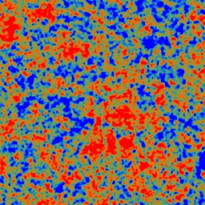
Figure 4.5: Recovery of the SZ signal with Planck. Top-Left: SZ effect in the $\Lambda$CDM assuming pressure traces dark matter density field with a scale independent bias. The field is $6^{\circ}\times 6^{\circ}$ and the range of the map is $-100\mu K,25\mu K$ with an rms of $9\mu K$ and has an approximate angular resolution of $2^{\prime}$. Note the lack of obvious filamentary structures. Form top-left to to bottom-left, model SZ signal with first map smoothed with a top-hat of radius $20^{\prime}$, signal $+$ noise from primary anisotropies and foregrounds, and final recovered map from Planck.

As examples, we have employed the frequency and noise specifications of the Boomerang, MAP, Planck experiments. The MAP satellite only covers frequencies at RJ part of the frequency spectrum. Consequently, only Boomerang and Planck can take full advantage of multifrequency separation of the SZ and primary anisotropies. We have evaluated the detection threshold for SZ power spectrum measurements (see Fig. 4.4). In Fig. 4.5, we demonstrate the ability of Planck mission to produce a map of the SZ effect using the frequency information. Boomerang and MAP should provide limits on the degree scale fluctuations at the several $\mu$K level in rms; Planck should be able to detect sub $\mu$K signals. This statement is independent of our assumptions about the SZ effect, including the non-Gaussianity. The exact detection threshold, however, depends on the assumptions associated with foreground distribution, including whether the foregrounds can be modeled as a Gaussian distribution.

In the next few sections, we will turn to the question on the exact SZ contribution. Since at large scales, the SZ effect can be well modeled with a model in which gas traces the density field with a bias, we can use such a simplified approach to obtain an order of magnitude estimate on the signal-to-noise for the detection of the SZ power spectrum (see, [Cooray et al.] 2000a). We summarize our results in Fig. 4.6. As shown, Planck mission as the greatest potential to detect the SZ effect at large scales while MAP and Boomerang allow useful upper limits on few sigma detections.

In the next section, we use the basic fact that SZ effect traces pressure fluctuations in the universe and study clustering properties of large scale pressure under the halo model. We use these predictions for pressure power spectrum and higher order correlations to study the angular power spectrum, bispectrum and trispectrum of the SZ effect.

Figure 4.6: Cumulative signal-to-noise in the measurement of the SZ power spectrum with Boomerang, MAP and Planck as a function of maximum $l$. The solid line is the maximum signal-to-noise achievable in a perfect experiment with no instrumental noise and full-sky coverage.

4.3 Clustering Properties of Pressure

Following [Scoccimarro et al.] (1999), we can relate the trispectrum to the variance of the estimator of the binned power spectrum

$$\hat{P}_{i}={1\over V}\int_{{\rm s}i}{d^{3}k\over V_{{\rm s}i}}\Pi^{*}(-{\bf k})\Pi({\bf k})\,,$$ (4.13)

where the integral is over a shell in $k$-space centered around $k_{i}$, $V_{{\rm s}i}\approx 4\pi k_{i}^{2}\delta k$ is the volume of the shell and $V$ is the volume of the survey. Recalling that $\delta({\bf 0})\rightarrow V/(2\pi)^{3}$ for a finite volume,

$$C_{ij} \equiv \left<\hat{P}_{i}\hat{P}_{j}\right>-\left<\hat{P}_{i}\right>\left<\hat{P}_{j}\right>$$ (4.14)

$$= {1\over V}\left[{(2\pi)^{3}\over V_{{\rm s}i}}2P_{i}^{2}\delta_{ij}+T_{ij}^{\Pi}\right]\,,$$

where

$$T_{ij}^{\Pi} \equiv \int_{{\rm s}i}{d^{3}k_{i}\over V_{{\rm s}i}}\int_{{\rm s}j}{d^{3}k_{j}\over V_{{\rm s}j}}T_{\Pi}({\bf k}_{i},-{\bf k}_{i},{\bf k}_{j},-{\bf k}_{j})\,.$$ (4.15)

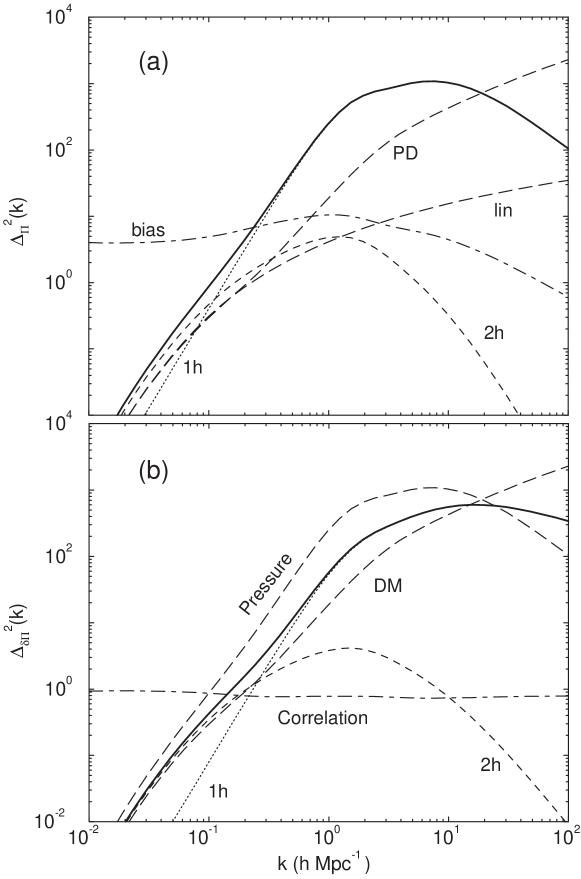
Figure 4.7: The pressure power spectrum (a) and the cross-power spectrum between pressure and dark matter (b) today ($z=0$) broken into individual contributions under the halo description. The lines labeled ’bias’ and “correlations” shows the pressure bias and correlation relative to the dark matter power spectrum under the halo model. The pressure behaves such that it correlates well with dark matter at large scales while there is a breakdown in this correlation at small scales.

Notice that though both terms scale in the same way with the volume of the survey, only the Gaussian piece necessarily decreases with the volume of the shell. For the Gaussian piece, the sampling error reduces to a simple root-N mode counting of independent modes in a shell. The trispectrum quantifies the non-independence of the modes both within a shell and between shells. Calculating the covariance matrix of the power spectrum estimates reduces to averaging the elements of the trispectrum across configurations in the shell.

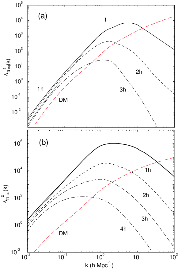
Figure 4.8: The pressure bispectrum (a) and the trispectrum today ($z=0$) broken into individual contributions under the halo description. Here, we show the equilateral configuration for the bispectrum and square configuration for the trispectrum. For comparison, we also show the dark matter bispectrum and trispectrum, under the halo model, for the same configurations.

$k$	0.06	0.07	0.09	0.11	0.14	0.17	0.21	0.25	0.31
0.05	1.00	0.65	0.73	0.74	0.74	0.71	0.70	0.68	0.68
0.07	(0.06)	1.00	0.81	0.87	0.87	0.85	0.83	0.82	0.81
0.09	(0.12)	(0.10)	1.00	0.90	0.93	0.92	0.90	0.89	0.88
0.11	(0.18)	(0.19)	(0.16)	1.00	0.95	0.96	0.95	0.93	0.93
0.14	(0.25)	(0.30)	(0.29)	(0.28)	1.00	0.98	0.97	0.96	0.95
0.17	(0.30)	(0.37)	(0.37)	(0.43)	(0.43)	1.00	0.98	0.97	0.96
0.21	(0.33)	(0.33)	(0.41)	(0.54)	(0.58)	(0.59)	1.00	0.98	0.97
0.25	(0.34)	(0.34)	(0.42)	(0.58)	(0.69)	(0.74)	(0.75)	1.00	0.99
0.31	(0.33)	(0.33)	(0.41)	(0.57)	(0.70)	(0.78)	(0.84)	(0.86)	1.00
$\sqrt{\frac{C_{ii}}{C_{ii}^{G}}}_{\rm\Pi}$	1.29	1.64	1.95	2.24	3.58	6.09	9.27	16.4	21.2
$\sqrt{\frac{C_{ii}}{C_{ii}^{G}}}_{\rm\delta}$	1.02	1.03	1.04	1.07	1.14	1.23	1.38	1.61	1.90

Table 4.2: Diagonal normalized covariance matrix of the binned pressure (upper triangle) and dark matter density field (lower triangle) power spectrum with $k$ values in units of h Mpc^-1. Lower triangle (parenthetical numbers) displays the covariance from halo model in [Cooray & Hu] (2001b). Final line shows the fractional increase in the errors (root diagonal covariance) due to non-Gaussianity as calculated under the halo model for pressure and dark matter density field.

4.3.1 Discussion

In Fig. 4.7(a), we show the logarithmic power spectrum of pressure and dark matter such that $\Delta^{2}(k)=k^{3}P(k)/2\pi^{2}$ with contributions broken down to the $1h$ and $2h$ terms today. As shown, the pressure power spectrum depicts an increase in power relative to the dark matter at scales out to few h Mpc^-1, and a decrease thereafter. The decrease in power at small scales can be understood through the relative contribution to pressure as a function of the halo mass.

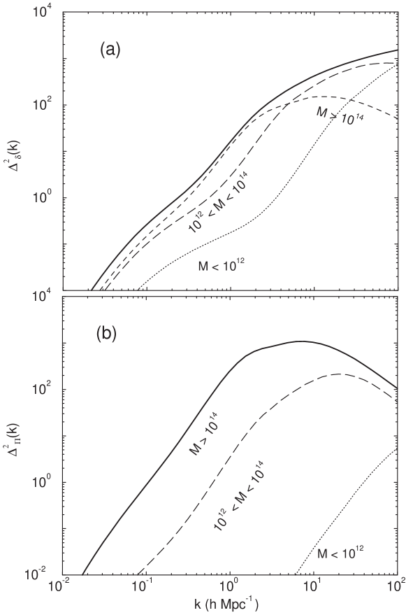
Figure 4.9: The mass dependence on the dark matter power spectrum (a) and pressure power spectrum (b). Here, we show the total contribution broken in mass limits as written on the figure. As shown in (a), the large scale contribution to the dark matter power comes from massive halos while small mass halos contribute at small scales. For the pressure, in (b), only massive halos above a mass of $10^{14}$ M_sun contribute to the power.

In Fig. 4.9, we break the total dark matter power spectrum (a) and the total pressure power spectrum (b), to a function of mass. As shown, contributions to both dark matter and pressure comes from massive halos at large scales and by small mass halos at small scales. The pressure power spectrum is such that through temperature weighing, with $T_{e}\propto M^{2/3}$ dependence, the contribution from low mass halos to pressure is suppressed relative to that from the high mass end. Thus, the pressure power spectrum, at all scales of interest, can be easily described with halos of mass greater than $10^{14}$ $M_{\sun}$. A comparison of the dark matter and pressure power spectra, as a function of mass, in Fig. 4.9 reveals that the turn over in the pressure power spectrum results at an effective scale radius for halos with mass greater than $10^{14}$ M${}_{\sun}$. We refer the reader to [Cooray] (2000) for further details on the pressure power spectrum and its properties.

Similar to the electron temperature dependence on mass in pressure, the description of the galaxy power spectrum under the halo model, as discussed in § 1.7, is such that the number of galaxies as a function of mass has a functional description given by $N_{\rm gal}\propto M^{\alpha}$ with $\alpha\sim 0.7$ to 0.8 (see, [Scoccimarro et al.] 2000). However, there is a significant contribution from low mass halos at small angular scales since the description allows the formation of at least one galaxy in halo down to some low mass limit. Thus, contrary to the behavior in pressure, one finds that there is significant low halo mass contribution to the galaxy power spectrum. We can increase the contribution from low mass halos if we allow for a minimum temperature in electrons, such as due to non-gravitational or so-called preheating. Though we do not include such a minimum temperature here, we will address how one can observationally determine such a minimum temperature for electrons later.

For the covariance of pressure, and also for the covariance of the SZ power spectrum, we are mainly interested in terms of the pressure trispectrum involving configurations that result in $T_{\Pi}({\bf k}_{1},-{\bf k}_{1},{\bf k}_{2},-{\bf k}_{2})$, i.e. parallelograms which are defined by either the length $k_{12}$ or the angle between ${\bf k}_{1}$ and ${\bf k}_{2}$. For illustration purposes we will take $k_{1}=k_{2}$ and the angle to be $90^{\circ}$ (${\bf k}_{2}={\bf k}_{\perp}$) such that the parallelogram is a square. It is then convenient to define

$$\Delta^{2}_{\Pi\rm sq}(k)\equiv\frac{k^{3}}{2\pi^{2}}T_{\Pi}^{1/3}({\bf k},-{\bf k},{\bf k}_{\perp},-{\bf k}_{\perp})\,,$$ (4.16)

such that this quantity scales roughly as the logarithmic power spectrum itself $\Delta^{2}(k)$. This spectrum is shown in Fig. 4.8(b) with the individual contributions from the 1h, 2h, 3h, 4h terms shown. As shown, almost all contributions to the pressure trispectrum come from the single halo term.

Using the pressure trispectrum, we can now predict the pressure covariance and, more appropriately, correlations in the binned measurements of the pressure. The predictions made here with the halo model to describe pressure can easily be tested in numerical simulations and the accuracy of the halo model can be further studied. For this purpose, we calculate the covariance matrix $C_{ij}$ from Eq. 4.15 with the bins centered at $k_{i}$ and volume $V_{{\rm s}i}=4\pi k_{i}^{2}\delta{k_{i}}$. The binning scheme used here is the one we utilized in [Cooray & Hu] (2001b) to calculate the binned dark matter power spectrum correlations.

In Table 4.2, we tabulate the pressure (upper triangle), and for comparison dark matter (lower triangle), correlation coefficients

$$\hat{C}_{ij}={C_{ij}\over\sqrt{C_{ii}C_{jj}}}\,.$$ (4.17)

The dark matter correlations are from the halo based predictions by [Cooray & Hu] (2001b). There, for the dark matter, we suggested that the halo model predicted correlations agree with numerical simulations of [Meiksin & White] (1999) typically better than $\pm 0.1$, even in the region where non-Gaussian effects dominate, and that the the qualitative features such as the increase in correlations across the non-linear scale are preserved. As we do not have measurements of the pressure correlations from simulations, we cannot perform a detailed comparison on the accuracy of the halo model predictions for pressure here.

A further test on the accuracy of the halo approach is to consider higher order real-space moments such as the skewness and kurtosis. In [Cooray] (2000), we discussed the SZ skewness under the halo model. As discussed in detail by [Refregier & Teyssier] (2001), halo model predictions agree remarkably well with numerical simulations, especially for the pressure and SZ power spectra, though, detailed comparisons still remain to be made with respect to bispectrum and trispectrum.

Even though the dark matter halo formalism provides a physically motivated means of calculating the statistics of the dark matter density field and associated properties such as pressure, there are several limitations of the approach that should be borne in mind when interpreting results. The approach assumes all halos to share a parameterized spherically-symmetric profile and this assumption is likely to affect detailed results on the configuration dependence of the bispectrum and trispectrum. Since we are considering a weighted average of configurations, our predictions presented here may be insufficient to establish the validity of the trispectrum modeling in general. Further numerical work is required to quantify to what extent the present approach reproduces simulation results for the full trispectrum. We do not consider such comparisons here, other than to suggest that the halo model has provided, at least qualitatively, a consistent description better than any of the arguments involving a biased description of gas tracing the dark matter etc.

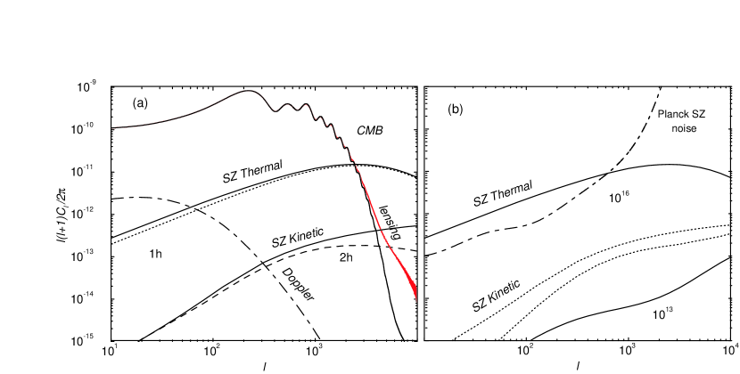
Figure 4.10: The angular power spectra of SZ thermal and kinetic effects. As shown in (a), the thermal SZ effect is dominated by individual halos, and thus, by the single halo term, while the kinetic effect is dominated by the large scale structure correlations depicted by the 2-halo term. In (b), we show the mass dependence of the SZ thermal and kinetic effects with a maximum mass of $10^{16}$ and $10^{13}$ M${}_{\sun}$. The SZ thermal effect is strongly dependent on the maximum mass, while due to large scale correlations, kinetic effect is not.

4.4 SZ Power Spectrum, Bispectrum and Trispectrum

The Sunyaev-Zel’dovich (SZ; [Sunyaev & Zel’dovich] 1980) effect arises from the inverse-Compton scattering of CMB photons by hot electrons along the line of sight. The temperature decrement along the line of sight due to SZ effect can be written as the integral of pressure along the same line of sight

$$y\equiv\frac{\Delta T}{T_{\rm CMB}}=g(x)\int dra(r)\frac{k_{B}\sigma_{T}}{m_{e}c^{2}}n_{e}(r)T_{e}(r)\,$$ (4.18)

where $\sigma_{T}$ is the Thomson cross-section, $n_{e}$ is the electron number density, $r$ is the comoving distance, and $g(x)=x{\rm coth}(x/2)-4$ with $x=h\nu/k_{B}T_{\rm CMB}$ is the spectral shape of SZ effect. At Rayleigh-Jeans (RJ) part of the CMB, $g(x)=-2$. For the rest of this paper, we assume observations in the Rayleigh-Jeans regime of the spectrum; an experiment such as Planck with sensitivity beyond the peak of the spectrum can separate out these contributions based on the spectral signature, $g(x)$ ([Cooray et al.] 2000a).

The SZ power spectrum, bispectrum and trispectrum are defined in the flat sky approximation in the usual way

$$\left<y({\mathbf{l}}_{1})y({\mathbf{l}}_{2})\right> = (2\pi)^{2}\delta_{\rm D}({\mathbf{l}}_{12})C_{l}^{\rm SZ}\,,$$

$$\left<y({\mathbf{l}}_{1})y({\mathbf{l}}_{2})y({\mathbf{l}}_{3})\right>_{c} = (2\pi)^{2}\delta_{\rm D}({\mathbf{l}}_{123})B^{\rm SZ}({\mathbf{l}}_{1},{\mathbf{l}}_{2},{\mathbf{l}}_{3})\,,$$

$$\left<y({\mathbf{l}}_{1})\ldots y({\mathbf{l}}_{4})\right>_{c} = (2\pi)^{2}\delta_{\rm D}({\mathbf{l}}_{1234})T^{\rm SZ}({\mathbf{l}}_{1},{\mathbf{l}}_{2},{\mathbf{l}}_{3},{\mathbf{l}}_{4})\,.$$ (4.19)

These can be written as a redshift projection of the pressure power spectrum, bispectrum and trispectrum, respectively:

$$C_{l}^{\rm SZ} = \int dr\frac{W^{\rm SZ}(r)^{2}}{d_{A}^{2}}P_{\Pi}^{\rm t}\left(\frac{l}{d_{A}},r\right)\,,$$ (4.20)

$$B^{\rm SZ} = \int dr\frac{W^{\rm SZ}(r)^{3}}{d_{A}^{4}}B_{\Pi}\left(\frac{{\mathbf{l}}_{1}}{d_{A}},\frac{{\mathbf{l}}_{2}}{d_{A}},\frac{{\mathbf{l}}_{3}}{d_{A}},;r\right)\,,$$

$$T^{\rm SZ} = \int dr\frac{W^{\rm SZ}(r)^{4}}{d_{A}^{6}}T_{\Pi}\left(\frac{{\mathbf{l}}_{1}}{d_{A}},\frac{{\mathbf{l}}_{2}}{d_{A}},\frac{{\mathbf{l}}_{3}}{d_{A}},\frac{{\mathbf{l}}_{4}}{d_{A}},;r\right)\,.$$ (4.21)

Here, $d_{A}$ is the angular diameter distance. At RJ part of the frequency spectrum, the SZ weight function is

$$W^{\rm SZ}(r)=-2\frac{k_{B}\sigma_{T}\bar{n}_{e}}{a(r)^{2}m_{e}c^{2}}$$ (4.22)

where $\bar{n}_{e}$ is the mean electron density today. In deriving Eq. 4.21, we have used the Limber approximation [Limber] by setting $k=l/d_{A}$ and flat-sky approximation.

4.4.1 Discussion

Figure 4.11: Flat band power in the fiducial $\Lambda$CDM model with the pressure power spectrum related to a filtered version of the non-linear dark matter power spectrum (dotted lines). From top to bottom $k_{F}=\infty,10,5,2,1,0.5,0.2$. With a dashed line, we have also shown the SZ power spectrum derived in typical numerical simulations (e.g., [Seljak et al.] 2000). The solid line shows the prediction based on the halo approach. We also plot the 68% confidence on a preliminary detection of anisotropies at small angular scales using the BIMA interferometer by [Dawson et al.] (2000).

In Fig. 4.10(a), we show the SZ power spectrum due to baryons present in virialized halos. As shown, most of the contributions to SZ power spectrum comes from individual massive halos, while the halo-halo correlations only contribute at a level of 10% at large angular scales. This is contrary to, say, the lensing convergence power spectrum discussed in [Cooray et al] (2000b), where most of the power at large angular scales is due to the halo-halo correlations. The difference can be understood by noting that the SZ effect is strongly sensitive to the most massive halos due to $T\propto M^{2/3}$ dependence in temperature and to a lesser, but somewhat related, extent that its weight function increases towards low redshifts. The lensing weight function selectively probes the large scale dark matter density power spectrum at comoving distances half to that of background sources ($z\sim 0.2$ to 0.5 when sources are at a redshift of 1), but has no extra dependence on mass. The fact that the SZ power spectrum results mainly from the single halo term also results in a sharp reduction of power when the maximum mass used in the calculation is varied. For example, as discussed in [Cooray] (2000) and illustrated in Fig 4.10(b), with the maximum mass decreased from $10^{16}$ to $10^{13}$ M${}_{\sun}$, the SZ power spectrum reduced by a factor nearly two orders of magnitude in large scales and an order of magnitude at $l\sim 10^{4}$.

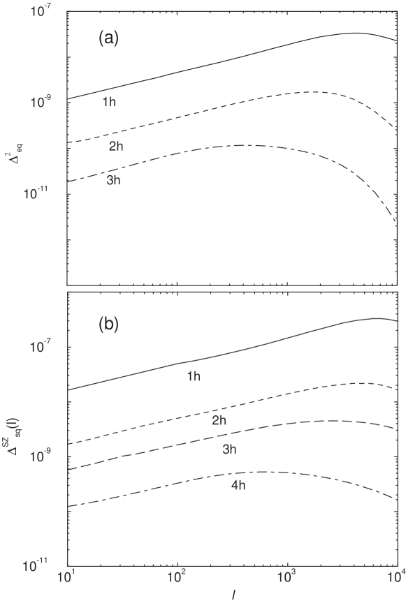
Figure 4.12: SZ bispectrum (a) and trispectrum (b) for configurations that involve equilateral triangles and squares, respectively, under the halo model. As shown, single halo term dominates the contribution to bispectrum and trispectrum at all multipoles ranging from large angular scales to small angular scales. The dependence on the single halo term is consistent with the general non-Gaussian behavior of the SZ effect and its significant non-linearity.

In addition to the halo model, we can also consider another semianalytic approach to calculate the SZ power spectrum using a filtered version of the non-linear dark matter power spectrum. It is well known that the non-linear effects generally enhances power at small scales, though, due to pressure cut-off clustering of pressure is not expected to occur down to smallest scales. In fact, Pen (1999), based on his simulations and numerical calculations, argue that large scale structure gas does not cluster at scales less than $\sim$ 850 kpc. Similar cutoffs due to pressure has also been studied in Gnedin & Hui (1998) using various filtering mechanisms. To get a qualitative understanding of any filtering effects of the gas power spectrum on the SZ effect, we consider a simple filtered version of the gas power spectrum given by

$$P^{\rm fil}_{\Pi}(k)=\exp(-k^{2}/k_{F}^{2})b^{2}_{\Pi}P_{\delta}(k)$$ (4.23)

where $k_{F}$ is the filtering scale and $b_{\Pi}$ is the large scale bias of pressure related to the non-linear dark matter power spectrum. Here, we use the constant bias value at large scales. The resulting temperature fluctuations for the SZ power spectrum for various numerical values of $k_{F}$ are shown in Fig. 4.11. For comparison, we also show prediction based on the halo model and predictions generally from numerical simulations; Note that simulations underestimate the SZ effect at large scales due to numerical issues related to volume of the simulation and resolution. As shown, a constant bias with a filtering scheme for the non-linear power spectrum does not fully produce the halo model. Of course, if one uses the scale dependent bias (as shown in Fig. 4.7), the non-linear dark matter power spectrum produces the SZ effect with no filtering. In Fig. 4.11, we also show a recent preliminary detection of the temperature fluctuations at small angular scales by [Dawson et al.] (2000). With improvements in the experimental side, it is likely that future measurements of the SZ power spectrum will greatly constrain the underlying physics that generate the temperature fluctuations. We will discuss such a possibility with the generation of the full SZ covariance, including non-Gaussianities.

Figure 4.13: The fractional errors in the measurements of the SZ band powers. Here, we show the fractional errors under the Gaussian approximation, and the total including non-Gaussianities. As shown, the total contribution as a function of mass is sensitive to the presence of most massive halos in the universe. The non-Gaussian term is essentially dominated by the single halo term.

Figure 4.14: The non-Gaussian correlation coefficient $\hat{C}_{ij}^{\rm NG}$, of the SZ power spectrum, involving only the configuration of the SZ trispectrum that contribute to the SZ power spectrum covariance (see, Eq. 4.30). The correlations are such that they tend to 1 as $l_{i}\rightarrow l_{j}$ and is fully described by the contribution to the trispectrum by the single halo term.

4.5 SZ Power Spectrum Covariance

For the purpose of this calculation, we assume that upcoming weak lensing convergence power spectrum will measure binned logarithmic band powers at several $l_{i}$’s in multipole space with bins of thickness $\delta l_{i}$.

$${\cal C}_{i}=\int_{{\rm s}i}{d^{2}l\over{A_{{\rm s}i}}}\frac{l^{2}}{2\pi}y(\bf l)y(-\bf l)\,,$$ (4.24)

where $A_{\rm s}(l_{i})=\int d^{2}l$ is the area of the two-dimensional shell in multipole and can be written as $A_{\rm s}(l_{i})=2\pi l_{i}\delta l_{i}+\pi(\delta l_{i})^{2}$.

We can now write the signal covariance matrix as

$$C_{ij} = {1\over A}\left[{(2\pi)^{2}\over A_{{\rm s}i}}2{\cal C}_{i}^{2}+T^{\rm SZ}_{ij}\right]\,,$$ (4.25)

$$T^{\rm SZ}_{ij} = \int{d^{2}l_{i}\over A_{{\rm s}i}}\int{d^{2}l_{j}\over A_{{\rm s}j}}{l_{i}^{2}l_{j}^{2}\over(2\pi)^{2}}T^{\rm SZ}({\mathbf{l}}_{i},-{\mathbf{l}}_{i},{\mathbf{l}}_{j},-{\mathbf{l}}_{j})\,,$$ (4.26)

where $A$ is the area of the survey in steradians. Again the first term is the Gaussian contribution to the sample variance and the second term is the non-Gaussian contribution. A realistic survey will also have an additional noise variance due to the instrumental effects and a covariance resulting from the uncertainties associated with the separation of the SZ effect from thermal CMB and other foregrounds.

$\ell_{\rm bin}$	529	739	1031	1440	2012	2802	3905	5432	7568
529	1.00	0.88	0.69	0.48	0.30	0.17	0.17	0.11	0.07
739	(0.00)	1.00	0.88	0.68	0.49	0.38	0.28	0.20	0.13
1031	(0.00)	(0.00)	1.00	0.87	0.68	0.56	0.43	0.31	0.21
1440	(0.00)	(0.00)	(0.00)	1.00	0.88	0.69	0.61	0.45	0.31
2012	(0.00)	(0.00)	(0.01)	(0.05)	1.00	0.88	0.69	0.60	0.42
2802	(0.00)	(0.00)	(0.02)	(0.09)	(0.39)	1.00	0.88	0.70	0.56
3905	(0.00)	(0.00)	(0.02)	(0.08)	(0.36)	(0.84)	1.00	0.87	0.70
5432	(0.00)	(0.00)	(0.01)	(0.06)	(0.29)	(0.65)	(0.86)	1.00	0.88
7568	(0.00)	(0.00)	(0.01)	(0.04)	(0.20)	(0.53)	(0.70)	(0.88)	1.00

Table 4.3: Covariance of the binned power spectrum for the SZ effect. Upper triangle displays the covariance found when a perfect frequency cleaned SZ map is used to determine the SZ power spectrum. Lower triangle (parenthetical numbers) displays the covariance found when the variance is dominated by the primary anisotropy contribution, as in a measurement of the SZ power spectrum in a CMB primary fluctuations dominated map.

In Fig 4.12(b), we show the scaled trispectrum

$$\Delta^{\rm SZ}_{\rm sq}(l)=\frac{l^{2}}{2\pi}T^{\rm SZ}({\bf l},-{\bf l},{\bf l}_{\perp},-{\bf l}_{\perp})^{1/3}\,.$$ (4.27)

where $l_{\perp}=l$ and ${\bf l}\cdot{\bf l}_{\perp}=0$. The projected SZ trispectrum again shows the same behavior as the pressure trispectrum with similar conditions on ${\bf k}_{i}$’s. As shown, the contributions to the trispectrum essentially comes from the single halo term at all multipoles. This is consistent with our observation that SZ power spectrum is essentially dominated by the correlations of pressure within halos. As discussed in [Cooray] (2000), and shown in Fig. 4.12(a), the SZ bispectrum, shown here for the equilateral triangular configuration such that $l_{1}=l_{2}=l_{3}=l$, is also dominated by the single halo term. Given this dependence on the single halo term, for the rest of the discussion involving SZ covariance, we will only use the single halo term and ignore the contributions arising from large scale correlations associated with halos.

We can now use this trispectrum to study the contributions to the covariance, which is what we are primarily concerned here. In Fig. 4.13, we show the fractional error,

$${\Delta{\cal C}_{i}\over{\cal C}_{i}}\equiv{\sqrt{C_{ii}}\over{\cal C}_{i}}\,,$$ (4.28)

for bands $l_{i}$ given in Table 4.3 following the binning scheme used in [Cooray & Hu] (2001b) for the weak lensing power spectrum.

In Fig. 4.13, the dashed line shows the Gaussian error while the solid line shows the total covariance with the addition of the SZ trispectrum (Eq. 4.26). At all multipoles, the non-Gaussianities from the trispectrum dominates the variance. As we discussed for the power spectrum, however, a reduction in the maximum mass of the halos used for the SZ calculation leads to a sharp decreases in the non-Gaussianities. With a mass cut at 10¹⁴ $M_{\sun}$, shown by the dotted line, we see that the total variance is consistent with the Gaussian variance out to $l\sim 1000$.

We can now write the correlation between the bands as

$$\hat{C}_{ij}\equiv\frac{C_{ij}}{\sqrt{C_{ii}C_{jj}}}\,.$$ (4.29)

In Table 4.3 we tabulate the SZ correlations under the assumption that the SZ power spectrum is measured independently, say in a frequency cleaned map, (upper triangle) and is measured in the CMB primary dominated map (lower triangle). The correlations along individual columns increase (as one goes to large $l$’s or small angular scales) and the maximum values are reached at $l\sim 5000$ consistent with the general behavior of the trispectrum.

In Fig. 4.14, we show the non-Gaussian trispectrum correlation coefficient given by

$$\hat{C}^{\rm NG}_{ij}=\frac{T_{ij}}{\sqrt{T_{ii}T_{ij}}}\,.$$ (4.30)

As shown here, the coefficient increases to higher $l$ to a maximum value of unity. The gradual increase is consistent with the fact that at all scales its the single halo term that dominates the non-Gaussian contribution. Since the power spectrum is dominated by correlations in single halos, the fixed profile of the halos correlate the power in all the modes and the correlations between adjacent modes are significant.

The calculation, or experimental measurement, of the full SZ covariance is necessary for the interpretation of observational results on the power spectrum. The upcoming SZ surveys, where the power spectrum will be measured, is likely to be limited to a small area on the sky. Thus, in the absence of many fields where the covariance can be estimated directly from the data, the halo model based approach suggested here provides a useful, albeit model dependent, quantification of the covariance. As suggested for weak lensing observations in [Hu & White] (2000) and discussed in [Cooray & Hu] (2001b), as a practical approach one could imagine taking the variances estimated from the survey under a Gaussian approximation, after accounting for uneven sampling and edge effects, and scaling it up by the non-Gaussian to Gaussian variance ratio of the halo model along with inclusion of the band power correlations. Additionally, using the covariance as the one calculated here, one can use the approach well known in the fields of CMB and galaxy power spectrum measurements to decorrelate band powers (e.g., [Hamilton] 1997; [Hamilton & Tegmark] 2000).

4.6 Astrophysical Uses of the SZ Power Spectrum

The calculation of the full covariance matrix now allows us to study how well the SZ power spectrum measures certain astrophysical and cosmological parameters. The upcoming CMB power spectrum measurements, complemented by the related local universe observations such as the galaxy power spectrum or supernovae, are expected to constrain most of the cosmological parameters to a reasonable accuracy (e.g., [Eisenstein et al.] 2000). Thus, we ignore the possibility that the SZ effect can be used as a probe of cosmology and only concentrate on the astrophysical uses of the SZ effect. This is a reasonable approach to take since there are many unknown astrophysics associated with the SZ effect involving the clustering of gas and its temperature. Such an approach allows us not to complicate the parameter measurements by adding both astrophysical and cosmological parameters. Assuming the cosmology will be safely known, we now ask the question what additional astrophysical parameters one can hope to extract from the SZ effect under the present halo model.

There are many approaches to parameterize the unknown astrophysics of the SZ power spectrum. Some possibilities have already been suggested in the literature, essentially involving the gas evolution (e.g., [Holder & Carlstrom] 1999; [Majumdar] 2001). Since the SZ effect involves both gas and temperature as a product, ie. the pressure, one may be led to conclude that it is not possible to separate effects associated with temperature from those associated with gas. Given the dependence of temperature on the pressure profile, independent of gas, however, it is expected that this degeneracy between gas properties and temperature effects can be partly broken.

As discussed earlier, the clustering of pressure power spectrum has a turnover corresponding to an equivalent scale radius of pressure. Through the gas pressure profile, this turn over can be characterized by the parameter $b$ and the dark matter scale radius $r_{s}$. Note that $b\propto 1/T_{e}$, so its measurement is essentially a probe of the electron temperature, though, it is unlikely that one can obtain all information on temperature and its evolution from one parameter measurement. Thus, instead of $b$, we take temperature itself to be one interesting astrophysical parameter and consider its evolution such that

$$T(M,z)=T_{0}\left(\frac{M}{10^{15}h^{-1}M_{\sun}}\right)^{T_{1}}(1+z)^{T_{\rm evol}}+T_{\rm min}\,.$$ (4.31)

Here, the four parameters represent the temperature-mass normalization, $T_{0}$, which in the fiducial case has the value given by the virial equation, the mass dependence slope, $T_{1}$, with a fiducial value of $2/3$, an redshift dependent evolutionary parameter, $T_{\rm evol}$, with a fiducial value of 1, and a minimum temperature for gas independent of mass and redshift $T_{\rm min}$, with a value of zero in the fiducial case. This latter parameter accounts for any possible preheating of gas before virializing in halos due to effects associated with some unknown astrophysics, such as the reionization process. A measurement of $T_{\rm min}$ would be interesting given that observational data from clusters to cluster groups suggest possible preheating of gas before virialization in halos. We note here that a redshift independent value for $T_{\rm min}$ may be too extreme since one expects preheating temperature to vary with redshift and mass such that all three parameters, $T_{0}$, $T_{1}$ and $T_{\rm evol}$, are affected. Still, we interested in the possibility of knowing how well we can establish a mass independent temperature value such as $T_{\rm min}$ through the SZ angular power spectrum. In Fig. 4.15, we show the variation in the redshift evolution of the density weighted temperature of electrons about the fiducial model. The density weight temperature was calculated following Eq. 1.76.

Figure 4.15: The variation in the density weighted temperature of electron as a function of redshift. The solid line shows the redshift evolution of the temperature under the fiducial model while variations about this model are shown as labeled.

In addition to the temperature, the SZ effect also depends on the number density of electrons in clusters. So far, we have considered this number through the universal baryon fraction in the universe such that $f_{g}\equiv M_{g}/M_{\delta}=\Omega_{g}/\Omega_{m}$. This assumption ignores any possible effects associated with the evolution of the gas fraction in halos, independent of any evolution that may be associated with temperature. It’ll be interesting to study to what extent future observations will allow the measurement of the fraction of baryons that is responsible for the SZ effect, and any evolution that may be associated with this fraction. Thus, a second set of parameters one can hope to extract from SZ observations involves gas mass fraction of halos and its evolution.

To study such gas properties, we parameterize the gas mass fraction such that

$$f_{g}=f_{0}\left(\frac{M}{10^{15}h^{-1}M_{\sun}}\right)^{f_{1}}(1+z)^{f_{\rm evol}}\,.$$ (4.32)

In a recent paper, [Majumdar] (2001) has suggested the strong possibility a measurement of any mass and redshift dependence of gas mass fraction in clusters, given that the SZ power spectrum was observed to vary significantly with changes in these two parameters. Since the SZ power spectrum essentially is sensitive to $\sim f_{g}^{2}T_{e}^{2}$, however, such a suggestion for measurement of gas evolution is not independent of any variations associated with temperature, which was ignored in the study of [Majumdar] (2001; also, [Holder & Carlstrom] 1999). Our general parameterization above involving both temperature and gas allows us to quantify how well independent statements can be made on possible measurement of gas density and temperature evolution, under the assumption that cosmology is known. Note that gas evolution is not present in our fiducial model since we take the gas fraction to be independent of mass and redshift with $f_{1}=0$ and $f_{\rm evol}=0$, respectively.

We now have a total of seven parameters we wish to extract from a measurement of the SZ power spectrum. In order to perform this calculation we take a Fisher matrix based approach. The Fisher matrix is simply a projection of the covariance matrix onto the basis of astrophysical parameters $p_{i}$ (see, Eq. 3.11). Note that under the approximation of Gaussian shot noise, the covariance reduces to replacing $C^{\rm SZ}_{l}\rightarrow C^{\rm SZ}_{l}+C^{\rm Noise}_{l}$ in the expressions leading up to the covariance Eq. 4.26. The noise power spectrum includes the noise associated with detectors, beam size and variance resulting from the separation of the SZ effect from other temperature fluctuations in multifrequency data.

Under the approximation that there are a sufficient number of modes in the band powers that the distribution of power spectrum estimates is approximately Gaussian, the Fisher matrix quantifies the best possible errors on cosmological parameters that can be achieved by a given survey. In particular $F^{-1}$ is the optimal covariance matrix of the parameters and $(F^{-1})_{ii}^{1/2}$ is the optimal error on the $i$th parameter. Implicit in this approximation of the Fisher matrix is the neglect of information from the parameter dependence of the covariance matrix of the band powers themselves. We neglect this information due to computational restrictions on the calculation of covariance for all variations in parameters within a reasonable amount of time. We do not expect this exclusion to change our results significantly. Also, here, we are mostly interested in an order of magnitude estimate on how well the SZ power spectrum can constrain astrophysics associated with large scale pressure.

The Fisher matrix approach allows us to address how well degeneracies are broken in the parameter space and under the assumption of a fiducial model for the parameters. For the purpose of this calculation, we take binned measurements of the SZ power spectrum following the binning scheme in Table 2. We consider a perfect SZ experiment with no noise contribution to the covariance and observations out to $l\sim 10^{4}$. To consider a real world scenario, we also study the astrophysical uses of the SZ power spectrum that can be extracted from the Planck mission. Here, we use the SZ noise power spectrum calculated for Planck with detector noise and uncertainties in the separation of SZ from CMB and other foreground in [Cooray et al.] (2000a). This SZ noise power spectrum is shown in Fig. 4.10(b).

$p_{i}$	$T_{0}$	$T_{1}$	$T_{\rm evol}$	$T_{\rm min}$	$f_{0}$	$f_{1}$	$f_{\rm evol}$
$T_{0}$	8.80	1.32	3.67	-1.93	-0.21	-1.69	-3.36
$T_{1}$		0.51	1.08	-0.18	-0.04	-0.41	-0.07
$T_{\rm evol}$			2.69	-0.62	-0.11	-0.94	-2.11
$T_{\rm min}$				0.48	0.04	0.29	0.67
$f_{0}$					0.006	0.05	0.09
$f_{1}$						0.39	0.73
$f_{\rm evol}$							1.67

Table 4.4: Inverse Fisher matrix ($\times 10^{2}$) for the SZ effect with seven parameters and full non-Gaussian errors. The error on an individual parameter is the square root of the diagonal element of the Fisher matrix for the parameter while off-diagonal entries of the inverse Fisher matrix shows correlations, and, thus, degeneracies, between parameters. We have assumed a perfect experiment with a full sky survey ($f_{\rm sky}=1$). The seven parameters are described in § 3.3.

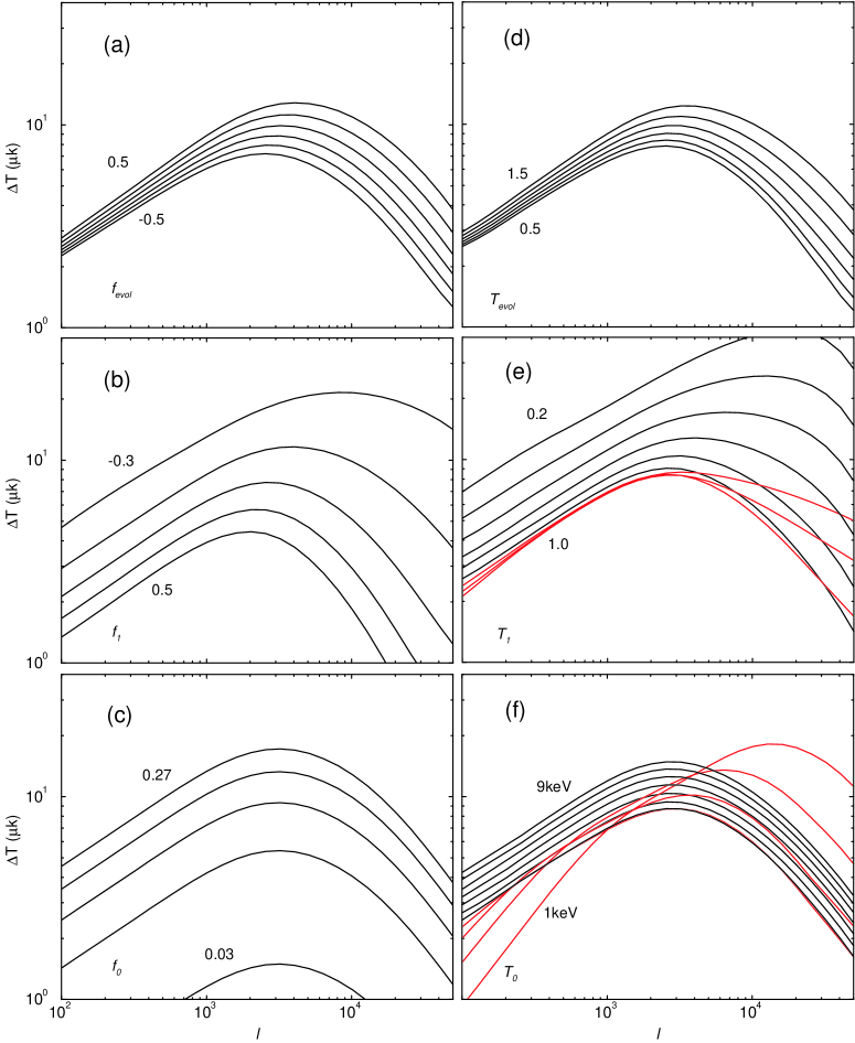
Figure 4.16: The temperature fluctuations of the SZ effect through variations in the astrophysical parameters under the halo model. From (a) to (c), we show the variations associated with gas evolution while from (d) to (f), we show variations involved with temperature. The parameters are described in § 3.3.

4.6.1 Discussion

In Fig. 4.16, we show the variation associated with SZ temperature fluctuations written such that $\Delta T=\sqrt{l(l+1)/(2\pi)C_{l}}T_{\rm CMB}$ for six of the seven parameters involved with gas, from (a) to (c), and temperature, (d) to (f), evolution. These plots allow us to understand some of the degeneracies associated with the description. For example, as shown, the gas and temperature redshift evolution essentially predicts similar behavior for the SZ temperature fluctuation, though there are minor differences due to the temperature dependence on the pressure profiles of halos. For the most part, variations due to temperature evolution is due to the normalization and not due to variations in the profile shape. In (b) and (e), we show variations due to the mass slope of the gas evolution and temperature evolution, respectively. Here again, we see similar behavior. When the slope of the mass-temperature relation, as a function of mass, is greater than 0.7, we see significant differences, especially involving an increase in temperature fluctuations at small scales. This is due to the relatively increasing weighing of small mass halos.

In (c) and (f), we show variations associated with gas evolution normalization $f_{0}$ and temperature-mass normalization $T_{0}$. The variation associated with $f_{0}$ is easily understood since the effect is only a change in the overall normalization of the power spectrum. The variation with temperature-mass normalization shows both effects due to normalization and the profile. When the normalization is low, gas clusters to small radii in low mass halos leading to an increase in power at small scales. As the temperature normalization is increased, gas profile varies such that there is a reduction in small scale power and the angular multipole of the turn-over scale shifts to low values. When the temperature normalization is sufficiently high, the overall weighing resulting from the overall temperature multiplicative factor becomes important. Now, the power spectrum behaves as a simple normalization change, similar to the variation in power due to gas evolution normalization. As shown in Fig. 4.16(a) to (f), there are significant degeneracies involved with astrophysical parameters that lead to the SZ effect.

In Table 4.5, we tabulate the errors on these seven parameters using the inverse Fisher matrix for a possible SZ power spectrum measurement. Here, we have considered the possibility that parameter extraction will be limited to 3, 5 and 7 parameters. The increase in number of parameters to be measured from a SZ power spectrum increases degeneracies associated with the set of parameters resulting in their accuracies. In the case of the 3 parameters involving temperature-mass normalization, $T_{0}$, a minimum temperature for all halos $T_{\rm min}$, and the gas mass fraction $f_{0}$, in a perfect experiment, all three parameters can be extracted such that they will be provide essentially very strong constraints. For example, the error on $f_{0}$ is such that one can identify the gas fraction of clusters responsible for SZ effect from the cosmic mean of $\Omega_{g}/\Omega_{m}=0.05/0.3$ with an error of $4\times 10^{-4}$. With Planck, one can constrain the preheating temperature at the level of $\sim$ 0.75 keV, and since current predictions for possible preheating is also at the level of few tenths keV, Planck SZ power spectrum can either confirm or put a useful limit on preheating temperature at current expectations.

As tabulated, however, the accuracy to which parameters can be determined from SZ power spectrum reduces significantly when the number of parameters to be determined is increased. For example, Planck mission will only set a limit at $\sim$ 1.7 keV, if one were to study both the mass and redshift dependence of electron temperatures. Such an upper limit is unlikely to be useful for current studies related to preheating of gas. Given that we cannot obtain useful errors with Planck for 5 parameters, we suggest that Planck may not be useful for the purpose of studying the full parameter space suggested here. This is understandable since Planck only allows the measurement of the SZ power spectrum out to $l\sim$ 1500, while most of the variations due to parameters under discussion here happens at $l\sim 5000$ where the turnover in the SZ power spectrum is observed. The Planck mission, however, allows one to obtain reasonable errors on parameters which generally define the normalization of the power spectrum, such as the temperature-mass normalization or the normalization of gas mass fraction. The normalization for gas mass fraction from Planck will be useful for the purpose of understanding what fraction of cosmic baryons reside in massive halos and contribute to the SZ effect and to look for any discrepancy of such a value from the total baryon content predicted by big bang nucleosynthesis arguments. In order to obtain reliable measurements of evolution of gas and temperature, a small scale experiment sensitive to multipoles out to $l\sim 10^{4}$ will be necessary.

For a perfect experiment, we show the errors on seven parameters also in Table 4.5. The inverse Fisher matrix in this case is tabulated in Table 4.4. The diagonals of the inverse Fisher matrix show the variance of individual parameters, while, more importantly, the off diagonals show the covariance between parameters. These covariances allow one to understand the degeneracies between parameters. In Table 4.5, we show the full extent to which parameters degrade the accuracies by tabulating degradation factors associated with the seven parameters. The degradation factor list the increase in parameter error from what can be achieved if all other parameters are known to what can be achieved when all parameters are to be retrieved from data. The degradation factors are at the level of one hundred or more for some parameters, suggesting that there are significant degeneracies associated with the parameterization of the temperature and gas fraction as a function of mass and redshift. Our result generally suggest that significant estimations of gas evolutionary properties, in the presence of unknown temperature properties, is not possible.

In addition to the parameter degeneracies, the non-Gaussianities associated with the SZ effect also increase the errors on parameters. For example, for the seven parameters under discussion here and again for a perfect and full sky experiment, we list the errors on parameters one can obtain if one were to ignore the non-Gaussian contributions to the covariance. As tabulated, non-Gaussianities increase the error on parameters by up to factors of 1.5, suggesting that the ignoring the non-Gaussianities will lead to a significant underestimate of the errors in parameters. This should be considered under the context that the SZ effect is significantly non-Gaussian at all scales of interest and that ability to distinguish parameters happen only at multipoles of a few thousand where the non-Gaussianities in fact dominate.

	$T_{0}$	$T_{1}$	$T_{\rm evol}$	$T_{\rm min}$	$f_{0}$	$f_{1}$	$f_{\rm evol}$
Perfect	0.04			0.002	0.0004
Planck	0.79			0.75	0.03
Perfect	0.13	0.02	0.06	0.05	0.002
Planck	1.39	0.41	1.22	1.37	0.05
Perfect	0.30	0.07	0.17	0.07	0.008	0.06	0.13
Degradation	47	184	133	34	82	240	130
Gaussian	0.18	0.04	0.10	0.04	0.005	0.04	0.08
Increase (%)	64	70	77	81	73	60	68

Table 4.5: Parameter errors, $(F^{-1})_{ii}^{1/2}$, using the halo model and the full covariance for the SZ effect. We tabulate these errors for a perfect experiment with no instrumental noise and full sky observations out to $l\sim 10^{4}$. We also show the expected errors for Planck mission with a useful sky fraction of 65% ($f_{\rm sky}=0.65$), and with the noise power spectrum shown in Fig. 4.10(b). The parameters are described in § 3.3. We break the parameter estimation to consider recovery of 3, 5 and 7 parameters. Under “Degradation” we tabulate the degradation factors, $(F)_{ii}^{-1/2}/(F^{-1})_{ii}^{1/2}$, due to parameter degeneracies. We also list the parameter errors expected if one were to assume Gaussian sample variance only for the SZ power spectrum and were to ignore the non-Gaussian covariance. The increase in error on individual parameters, with the introduction of the full covariance matrix, ranges from 40% to nearly 100%.

4.7 Weak Lensing-SZ Correlation: Non-Gaussianities in CMB

Large-scale structure deflects CMB photons in transit from the last scattering surface. These structures also give rise to secondary anisotropies. The result is a correlation between the temperature fluctuations and deflection angles. This effect cannot be seen in the two point function since gravitational lensing preserves surface brightness: deflections only alter the temperature field on the sky in the presence of intrinsic, primary, anisotropies in the unlensed distribution. The lowest order contribution thus comes from the three-point function or bispectrum.

In weak gravitational lensing, the deflection angle on the sky is given by the angular gradient of the lensing potential which is itself a projection of the gravitational potential (see e.g. [Kaiser] 1992),

$$\Theta(\hat{\bf m}) = -2\int_{0}^{r_{0}}dr\frac{d_{A}(r_{0}-r)}{d_{A}(r)d_{A}(r_{0})}\Phi(r,\hat{{\bf m}}r)\,.$$ (4.33)

This quantity is simply related to the more familiar convergence

$$\kappa(\hat{\bf m}) = {1\over 2}\nabla^{2}\Theta(\hat{\bf m})$$

$$= -\int_{0}^{r_{0}}dr\frac{d_{A}(r)d_{A}(r_{0}-r)}{d_{A}(r_{0})}\nabla_{\perp}^{2}\Phi(r,\hat{{\bf m}}r)\,,$$

where note that the 2D Laplacian operating on $\Phi$ is a spatial and not an angular Laplacian. The two terms $\kappa$ and $\Theta$ contain superficial differences in their radial and wavenumber weights which we shall see cancel in the appropriate Limber approximation. In particular, their spherical harmonic moments are simply proportional

$$\Theta_{lm} = -{2\over l(l+1)}\kappa_{lm}=\int d{\hat{\bf n}}Y_{l}^{m}{}^{*}(\hat{\bf n})\Theta(\hat{\bf n})$$ (4.35)

$$= i^{l}\int{d^{3}{\bf k}\over 2\pi^{2}}\delta({\bf k})Y_{l}^{m}{}^{*}(\hat{\bf k})I_{\ell}^{\rm def}(k)$$

with

$$I_{\ell}^{\rm def}(k) = \int_{0}^{r_{0}}drW^{\rm def}(k,r)j_{l}(kr)\,,$$

$$W^{\rm def}(k,r) = -3\Omega_{m}\left({H_{0}\over k}\right)^{2}F(r){d_{A}(r_{0}-r)\over d_{A}(r)d_{A}(r_{0})}\,.$$ (4.36)

Here, we have used the Rayleigh expansion of a plane wave (Eq. 2.8), and the fact that $\nabla^{2}Y_{l}^{m}=-l(l+1)Y_{l}^{m}$. In an open universe, one simply replaces the spherical Bessel functions with ultraspherical Bessel functions in expressions such as Eq. (4.36).

As pointed out by [Goldberg & Spergel] (1999), it does however have an effect on the bispectrum which is in principle observable. The lensed temperature fluctuation in a given direction is the sum of the primary fluctuation in a different direction plus the secondary anisotropy

$$T(\hat{\bf n}) = T^{\rm P}(\hat{\bf n}+\nabla\Theta)+T^{\rm S}(\hat{\bf n})$$

$$\approx \sum_{lm}\Big{[}(a_{lm}^{\rm P}+a_{lm}^{\rm S})Y_{l}^{m}(\hat{\bf n})+a_{lm}^{\rm P}\nabla\Theta(\hat{\bf n})\cdot\nabla Y_{l}^{m}(\hat{\bf n})\Big{]}\,,$$

or

$$a_{lm} = a_{lm}^{\rm P}+a_{lm}^{\rm S}+\sum_{l^{\prime}m^{\prime}}a_{l^{\prime}m^{\prime}}^{\rm P}\int d\hat{\bf n}Y_{l}^{m}{}^{*}(\hat{\bf n})\nabla\Theta(\hat{\bf n})\cdot\nabla Y_{l^{\prime}}^{m^{\prime}}(\hat{\bf n})\,.$$ (4.38)

Utilizing the definition of the bispectrum in Eq. 1.28, we obtain

$$B_{l_{1}l_{2}l_{3}} = \sum_{m_{1}m_{2}m_{3}}\left(\begin{array}[]{ccc}l_{1}&l_{2}&l_{3}\\ m_{1}&m_{2}&m_{3}\end{array}\right)$$ (4.42)

$$\times\int d\hat{\bf m}d\hat{\bf n}Y_{l_{2}}^{m_{2}}{}^{*}(\hat{\bf m})Y_{l_{3}}^{m_{3}}{}^{*}(\hat{\bf n})C_{l_{1}}\nabla Y_{l_{1}}^{m_{1}}{}^{*}(\hat{\bf m})\cdot\langle\nabla\Theta(\hat{\bf m})T^{\rm S}(\hat{\bf n})\rangle+{\rm Perm.}$$

where the five permutations are with respect to the ordering of $(l_{1},l_{2},l_{3})$.

Integrating by parts and simplifying further following [Goldberg & Spergel] (1999) leads to a bispectrum of the form:

$$B_{l_{1}l_{2}l_{3}}=-\left(\begin{array}[]{ccc}l_{1}&l_{2}&l_{3}\\ 0&0&0\end{array}\right)\sqrt{\frac{(2l_{1}+1)(2l_{2}+1)(2l_{3}+1)}{4\pi}}$$

$$\times \left[\frac{l_{2}(l_{2}+1)-l_{1}(l_{1}+1)-l_{3}(l_{3}+1)}{2}C_{l_{1}}b^{\rm S}_{l_{3}}+{\rm Perm.}\right]\,,$$

where we have employed Eq. 2.19 to perform the angular integration.

Figure 4.17: The power spectra of correlation between lensing deflections in CMB and the integrated Sachs-Wolfe effect ([Sachs & Wolfe] 1967) and the SZ thermal effect. The correlations are such that potentials responsible for the ISW effect correlate with lensing at large angular scales while SZ effect correlates with lensing at medium angular scales.

The quantity of interest here is the correlation between the deflection potential and the SZ effect, or any other secondary effect,

$$T^{\rm SZ}(\hat{\bf n})=\sum a_{lm}^{\rm SZ}Y_{l}^{m}(\hat{\bf n}),$$ (4.47)

which becomes

$$\langle\Theta(\hat{\bf n})T^{\rm SZ}(\hat{\bf m})\rangle = \sum_{lm}\left<\Theta_{lm}^{*}a_{lm}^{\rm SZ}\right>Y_{l}^{m}{}^{*}(\hat{\bf n})Y_{l}^{m}(\hat{\bf m})\,.$$ (4.48)

Statistical isotropy guarantees that we may write the correlation as

$$\left<\Theta_{lm}^{*}a_{lm}^{\rm SZ}\right> \equiv b_{l}\equiv{-2\over l(l+1)}C_{l}^{{\rm SZ}\kappa}\,,$$

$$= \frac{2}{\pi}\int k^{2}dkP_{\Pi\delta}(k)I_{l}^{\rm SZ}(k)I_{l}^{\rm def}(k)\,,$$

$$\approx \int\frac{dr}{d_{A}^{2}}W^{\rm SZ}(r)W^{\rm def}(r)P_{\Pi\delta}\left({l\over d_{A}}\right)\,,$$

where we have used Eq. 4.35 to relate the power spectrum $b_{l}$ defined by [Goldberg & Spergel] (1999) and the $\kappa$-secondary cross power spectrum defined by [Seljak & Zaldarriaga] (1999). The last line represents the Limber approximation.

The full signal-to-noise ratio of the bispectrum is

$$\left({S\over N}\right)^{2}=f_{\rm sky}\sum_{l_{1},l_{2},l_{3}}{B_{l_{1}l_{2}l_{3}}^{2}\over 6C_{l_{1}}^{\rm t}C_{l_{2}}^{\rm t}C_{l_{3}}^{\rm t}}\,,$$ (4.50)

where

$$C_{l}^{\rm tot}=C_{l}^{\rm SZ}+N_{l}\,.$$ (4.51)

Recall that the residual noise $N_{l}$ was defined in equation (4.11) and includes contributions from detector noise. We plot the bispectrum cumulative signal-to-noise as a function of signal $l_{3}$, summed over $l_{1}$ and $l_{2}$. We refer the reader to [Cooray & Hu] (2000) for a detailed discussion on the bispectrum, its variance and the calculation of signal-to-noise ratio.

4.8 Discussion

The SZ effect and weak gravitational lensing of the CMB both trace large-scale structure in the underlying density field. By measuring the correlation, one can directly test the manner in which gas pressure fluctuations trace the dark matter density fluctuations. The correlation vanishes in the two-point functions since the lensing does not affect an isotropic CMB due to conservation of surface brightness.

The same correlation manifests itself as a non-vanishing bispectrum in the CMB at RJ frequencies ([Goldberg & Spergel] 1999; [Cooray & Hu] 2000). Again the cosmic variance from the primary anisotropies presents an obstacle for detection of the effect above the several arcminute scale ($l\sim 2000$). With the multifrequency cleaning of the SZ map presented here one can enhance the detectability of the effect.

Consider the bispectrum composed of one $a_{lm}$ from the cleaned SZ map and the other two from the CMB maps. Call this the SZ-CMB-CMB bispectrum. The noise variance of this term will be reduced by a factor of $C_{l}^{\rm t}/C_{l}^{\Theta}$ compared with the CMB-CMB-CMB bispectrum. As one can see from Fig. 4.2 this can be up to a factor of $10^{3}$ in the variance. Details for the calculation of the CMB-CMB-CMB bispectrum are given in [Cooray & Hu] (2000). Here we have updated the normalization for SZ effect, taken $f_{{\rm sky}}=0.65$ for Planck’s useful sky coverage, and compared the $S/N$ of the two bispectra. As shown in Fig. 4.18, the measurement using foreground cleaned Planck SZ and CMB maps has a substantially higher signal-to-noise than that from using the Planck CMB map alone for multipoles $l\sim 10^{2}-10^{3}$.

Our simple model assumes that the pressure is correlated with lensing potentials through the halo model. Thus, to the extent that the lensing and SZ signals can be determined separately from other measurements, the cross-correlation can be used to constrain the stochastic nature of the bias.

Beyond the improvement in signal-to-noise, however, there is an important advantage in constructing the SZ-lensing bispectrum using SZ and CMB maps. A mere measurement of the bispectrum in CMB data can lead to simultaneous detection of non-Gaussianities through processes other than just SZ-lensing cross-correlation. As discussed in [Goldberg & Spergel] (1999) and extended in [Cooray & Hu] (2000), gravitational lensing also correlates with other late time secondary anisotropy contributors such as integrated Sachs-Wolfe (ISW; [Sachs & Wolfe] 1967) effect and the reionized Doppler effect. In addition to lensing correlations, non-Gaussianities can also be generated through reionization and non-linear growth of perturbations ([Spergel & Goldberg] 1999; [Goldberg & Spergel] 1999; [Cooray & Hu] 2000). Bispectrum measurements at a signle frequency can result in a confusion as to the relative contribution from each of these scenarios. In [Cooray & Hu] (2000), we suggested the possibility of using differences in individual bispectra as a function of multipoles, however, such a separation can be problematic given that these differences are subtle (e.g., Fig 6 of [Cooray & Hu] 2000).

The construction of the SZ-lensing bispectrum using SZ and CMB maps has the advantage that one eliminates all possibilities, other than SZ, that result in a bispectrum. For effects related to SZ, the cross-correlation of lensing and SZ should produce the dominant signal; as shown in [Cooray & Hu] (2000), bispectra signal through SZ and reionization effects, such as Ostriker-Vishniac (OV; [Ostriker & Vishniac] 1986), are considerably smaller.

Conversely, multifrequency cleaning also eliminates the SZ contribution from the CMB maps and hence a main contaminant of the CMB-CMB-CMB bispectrum. This assists in the detection of smaller signals such as the ISW-lensing correlation, Doppler-lensing correlation or the non-Gaussianity of the initial conditions. Such an approach is highly desirable and Planck will allow such detailed studies to be carried out.

A potential caveat is that as noted above, the full bispectrum in an all-sky satellite experiment will be difficult to measure. [Zaldarriaga & Seljak] (1999) have developed a reduced set of three-point statistics optimized for lensing studies, based on a two point reconstruction of the lensing-convergence maps from the products of temperature gradients. They show that most of the information is retained in these statistics. Multifrequency cleaning improves the signal-to-noise for these statistics by exactly the same factor as for the full bispectrum.

Figure 4.18: Cumulative signal-to-noise in the measurement of the SZ-weak gravitational lensing cross-correlation through the bispectrum measurement in CMB data. Compared are the expected signal-to-noise with (SZ-CMB-CMB) and without (CMB-CMB-CMB) multifrequency isolation of the SZ effect for Planck and a perfect/cosmic variance limited experiment. Multifrequency isolation provides additional signal-to-noise and the opportunity to uniquely identify the bispectrum contribution with the SZ effect.

The cross-correlation coefficient between the SZ effect and CMB weak lensing is relatively modest ($\sim$ 0.5, see [Seljak et al.] 2000). This is due to the fact that the SZ effect is a tracer of the nearby universe while CMB lensing is maximally sensitive to structure at $z\sim 3$. A higher correlation is expected if SZ is cross-correlated with an external probe of low redshift structure. [Peiris & Spergel] (2000) suggested the cross-correlation of MAP CMB data and Sloan galaxy data. An improved approach would be to use the Planck derived SZ map rather than a CMB map. Using a SZ map reduces noise from the primary anisotropies and guarantees that any detection is due to correlations with the SZ effect. Extending the calculations in [Peiris & Spergel] (2000) with the Planck generated SZ map, we find signal-to-noise ratios which are on average greater by a factor of $\sim$ 10 when compared to signal-to-noise values using MAP CMB map. In fact with redshifts for galaxies, Planck SZ map can be cross-correlated in redshifts bins to study the redshift evolution of the gas. Other promising possibilities include cross correlation with soft X-ray background measurements, as well as ultraviolet and soft X-ray absorption line studies.

Chapter 5 Kinetic Sunyaev-Zel’dovich effect

5.1 Introduction

Extending our calculation on the contribution of large scale structure gas distribution to CMB anisotropies through SZ effect, we also study an associated effect involving baryons associated with halos in the large scale structure. It is well known that the peculiar velocity of galaxy clusters, along the line of sight, also lead to a contribution to temperature anisotropies. This effect is commonly known as the kinetic, or kinematic, Sunyaev-Zel’dovich effect and arises from the baryon density modulation of the Doppler effect associated with the velocity field ([Sunyaev & Zel’dovich] 1980). Given that both density and velocity fields are involved, the kinetic SZ effect is essentially second order, where as the thermal SZ effect, involving scattering of CMB photons is first order. Though the kinetic SZ effect was first described in [Sunyaev & Zel’dovich] (1980) using massive galaxy clusters, the same effect has been introduced under a different context by Ostriker and Vishniac (OV; [Ostriker & Vishniac] 1986; also, [Vishniac] 1987). The OV effect has been described as the contribution to temperature anisotropies due to baryon modulated Doppler effect in the linear regime of fluctuations. The kinetic SZ effect can be considered as the OV effect extended to the non-linear regime of baryon fluctuations, however, it should be understood that the basic physical mechanism responsible for the two effects is the same and that there is no reason to describe them as separate contributions. For the purpose of this presentation, we will treat both OV effect and the SZ kinetic effect as one contribution, though it may be easier to think of OV as the linear contribution while kinetic SZ, extending to non-linear regime will contain the total contribution. Such a description has been provided in [Hu] (2000a).

We calculate the kinetic SZ/OV effect, hereafter simply referred to as the kinetic SZ effect, using the model we developed to study the thermal SZ effect. We further extend this calculation to consider the correlation between SZ thermal and SZ kinetic effects. Since there is no first order cross-correlation, the lowest order contribution to the correlation comes from a three-point function, or a bispectrum. We discussed this bispectrum in [Cooray & Hu] (2000). Here, we consider an additional possibility to measure the SZ thermal-kinetic cross-correlation via a two-point correlation function which involves squares of the temperature, instead of the usual temperature itself. The power spectrum of squared temperatures probes one aspect of the trispectrum resulting through the pressure-baryon cross-correlation probed separately by the thermal SZ and kinetic SZ effects, respectively. Here, we show that there is adequate signal-to-noise for a reliable measurement of the SZ thermal-SZ kinetic squared power spectrum measurement in upcoming small angular scale experiments.

The Ostriker-Vishniac effect arises from the second-order modulation of the Doppler effect by density fluctuations (Ostriker & Vishniac 1986; Vishniac 1987). Its nonlinear analogue is the kinetic SZ effect from large-scale structure (Hu 1999). Due to its density weighting, the kinetic SZ effect peaks at small scales: arcminutes for $\Lambda$CDM. For a fully ionized universe, contributions are broadly distributed in redshift so that the power spectra are moderately dependent on the optical depth $\tau$. Here, we assume an optical depth to ionization of 0.1, consistent with current upper limits on the reionization redshift from CMB (e.g., [Griffiths et al.] 1999) and other observational data (see, e.g., [Haiman & Knox] 1999 and references therein).

5.2 Calculational Method

The kinetic SZ temperature fluctuations, denoted as ${\rm kSZ}$, can be written as a product of the line of sight velocity and density

$$T^{\rm kSZ}(\hat{\bf n})=\int drg(r)\hat{\bf n}\cdot{\bf v}_{g}(r,\hat{\bf n}r)n_{e}(r,\hat{\bf n}r)\,.$$ (5.1)

The first order contribution here now comes from the velocity field with the mean number density of electrons, $n_{e}=\bar{n}_{e}$. This contribution is discussed in [Kaiser] (1984) where it was shown to be insignificant at small scales due to significant mode cancellations. It should be understood that, contrary to the common thought, this does not mean that the contribution to temperature fluctuations from the velocity field is exactly zero. As discussed in [Kaiser] (1984) and [Cooray & Hu] (2000), double scattering effects, which are again due to the the velocity fluctuations, leave a non-zero signal at large scales. Also, single scattering effects are sensitive to how one models the transition to reionization; if the transition is instantaneous mode cancellations are not exact leaving behind a non-zero signal. The contribution we show as “Doppler” in Fig. 4.10 due to velocity fields assume reionization at a redshift of $\sim$ 13 ($\tau=0.1$), and a width $\Delta z$ of 0.1 (see, [Cooray & Hu] 2000).

Including density fluctuations, the full contribution is

$$T^{\rm kSZ}(\hat{\bf n}) = \int drg(r)\hat{\bf n}\cdot{\bf v}_{g}(r,\hat{\bf n}r)\bar{n}_{e}(1+\delta_{e})(r,\hat{\bf n}r)$$

$$= -i\int drg\int\frac{d^{3}{\bf k}}{(2\pi)^{3}}\int\frac{d^{3}{\bf k}^{\prime}}{(2\pi)^{3}}\delta_{v}({\bf k}-{\bf k}^{\prime})\delta_{g}({\bf k^{\prime}})e^{i{\bf k}\cdot\hat{\bf n}r}\left[\hat{\bf n}\cdot\frac{{\bf k}-{\bf k}^{\prime}}{|{\bf k}-{\bf k}^{\prime}|^{2}}\right]\,,$$

Note that one can use the linear theory to obtain the large scale velocity field in terms of the linear dark matter density field. The multiplication between the velocity and density fields in real space has been converted to a convolution between the two fields in Fourier space. The second line only includes the contribution from $v\delta$ term since the $v$ term is the linear Doppler effect.

We can now expand out the temperature perturbation due to kinetic SZ effect, $T^{\rm kSZ}$, into spherical harmonics:

$$a_{lm}^{\rm kSZ} = -i\int d\hat{\bf n}\int dr\;(g)\int\frac{d^{3}{\bf k_{1}}}{(2\pi)^{3}}\int\frac{d^{3}{\bf k_{2}}}{(2\pi)^{3}}\delta_{v}({\bf k_{1}})\delta_{g}({\bf k_{2}})$$ (5.3)

$$\times e^{i({\bf k_{1}+k_{2}})\cdot\hat{\bf n}r}\left[\frac{\hat{\bf n}\cdot{\bf k}_{1}}{k_{1}^{2}}\right]Y_{l}^{m\ast}(\hat{\bf n})\,,$$

where we have symmetrizised by using ${\bf k}_{1}$ and ${\bf k}_{2}$ to represent ${\bf k}-{\bf k}^{\prime}$ and ${\bf k}^{\prime}$ respectively. Using

$$\hat{\bf n}\cdot{\bf k}=\sum_{m^{\prime}}\frac{4\pi}{3}kY_{1}^{m^{\prime}}(\hat{\bf n})Y_{1}^{m^{\prime}\ast}(\hat{{\bf k}})\,,$$ (5.4)

and the Rayleigh expansion (Eq. 2.8), we can further simplify and rewrite the multipole moments as

$$a_{lm}^{\rm kSZ}=-i\frac{(4\pi)^{3}}{3}\int dr\int\frac{d^{3}{\bf k}_{1}}{(2\pi)^{3}}\int\frac{d^{3}{\bf k}_{2}}{(2\pi)^{3}}\sum_{l_{1}m_{1}}\sum_{l_{2}m_{2}}\sum_{m^{\prime}}$$ (5.5)

$$\times(i)^{l_{1}+l_{2}}g\frac{j_{l_{1}}(k_{1}r)}{k_{1}}j_{l_{2}}(k_{2}r)\delta_{v}({\bf k_{1}})\delta_{g}({\bf k_{2}})Y_{l_{1}}^{m_{1}}(\hat{{\bf k}}_{1})Y_{1}^{m^{\prime}}(\hat{{\bf k}}_{1})Y_{l_{2}}^{m_{2}}(\hat{{\bf k}}_{2})$$

$$\times \int d\hat{\bf n}Y_{l}^{m\ast}(\hat{\bf n})Y_{l_{1}}^{m_{1}\ast}(\hat{\bf n})Y_{l_{2}}^{m_{2}\ast}(\hat{\bf n})Y_{1}^{m^{\prime}\ast}(\hat{\bf n})\,.$$

We can construct the angular power spectrum by considering $\langle a_{l_{1}m_{1}}a^{*}_{l_{2}m_{2}}\rangle$. Under the assumption that the temperature field is statistically isotropic, the correlation is independent of $m$, and we can write the angular power spectrum as

$$\langle a_{l_{1}m_{1}}^{*,{\rm kSZ}}a_{l_{2}m_{2}}^{\rm kSZ}\rangle=\delta^{\rm D}_{l_{1}l_{2}}\delta^{\rm D}_{m_{1}m_{2}}C_{l_{1}}^{\rm kSZ}\,.$$ (5.6)

The correlation can be written using

$$\langle a^{\ast,{\rm kSZ}}_{l_{1}m_{1}}a^{\rm kSZ}_{l_{2}m_{2}}\rangle=\frac{(4\pi)^{6}}{9}\int dr_{1}g\int dr_{2}g$$ (5.7)

$$\times \int\frac{d^{3}{\bf k_{1}}}{(2\pi)^{3}}\frac{d^{3}{\bf k_{2}}}{(2\pi)^{3}}\frac{d^{3}{\bf k_{1}^{\prime}}}{(2\pi)^{3}}\frac{d^{3}{\bf k_{2}^{\prime}}}{(2\pi)^{3}}\langle\delta_{v}({\bf k_{1}^{\prime}})\delta_{g}({\bf k_{2}^{\prime}})\delta_{\delta}^{\ast{\rm lin}}({\bf k_{1}})\delta_{g}^{\ast}({\bf k_{2}})\rangle$$

$$\times \sum_{l_{1}^{\prime}m_{1}^{\prime}l_{1}^{\prime\prime}m_{1}^{\prime\prime}m_{1}^{\prime\prime\prime}l_{2}^{\prime}m_{2}^{\prime}l_{2}^{\prime\prime}m_{2}^{\prime\prime}m_{2}^{\prime\prime\prime}}(-i)^{l_{1}^{\prime}+l_{1}^{\prime\prime}}(i)^{l_{2}^{\prime}+l_{2}^{\prime\prime}}j_{l_{2}^{\prime}}(k_{1}^{\prime}r_{2})\frac{j_{l_{2}^{\prime\prime}}(k_{2}^{\prime}r_{2})}{k_{2}^{\prime}}\frac{j_{l_{1}^{\prime}}(k_{1}r_{1})}{k_{1}}j_{l_{1}^{\prime\prime}}(k_{2}r_{1})$$

$$\times \int d\hat{\bf m}Y_{l_{2}m_{2}}(\hat{\bf m})Y_{l_{2}^{\prime}m_{2}^{\prime}}^{\ast}(\hat{\bf m})Y_{l_{2}^{\prime\prime}m_{2}^{\prime\prime}}^{\ast}(\hat{\bf m})Y_{1m_{2}^{\prime\prime\prime}}^{\ast}(\hat{\bf m})$$

$$\times \int d\hat{\bf n}Y_{l_{1}m_{1}}^{\ast}(\hat{\bf n})Y_{l_{1}^{\prime}m_{1}^{\prime}}(\hat{\bf n})Y_{l_{1}^{\prime\prime}m_{1}^{\prime\prime}}(\hat{\bf n})Y_{1m_{1}^{\prime\prime\prime}}(\hat{\bf n})$$

$$\times \int d\hat{{\bf k}_{1}^{\prime}}\int d\hat{{\bf k}_{2}^{\prime}}Y_{l_{2}^{\prime}m_{2}^{\prime}}(\hat{{\bf k}_{1}^{\prime}})Y_{1m_{2}^{\prime\prime\prime}}(\hat{{\bf k}_{2}^{\prime}})Y_{l_{2}^{\prime\prime}m_{2}^{\prime\prime}}(\hat{{\bf k}_{1}^{\prime}})$$

$$\times \int d\hat{{\bf k}_{1}}\int d\hat{{\bf k}_{2}}Y_{l_{1}^{\prime}m_{1}^{\prime}}^{\ast}(\hat{{\bf k}_{1}})Y_{1m_{1}^{\prime\prime\prime}}^{\ast}(\hat{{\bf k}_{1}})Y_{l_{1}^{\prime\prime}m_{1}^{\prime\prime}}^{\ast}(\hat{{\bf k}_{2}})\,.$$

We can separate out the contributions such that the total is made of correlations following $\langle v_{g}v_{g}\rangle\langle\delta_{g}\delta_{g}\rangle$ and $\langle v_{g}\delta_{g}\rangle\langle v_{g}\delta_{g}\rangle$ depending on whether we consider cumulants by combining ${\bf k}_{1}$ with ${\bf k}_{1}^{\prime}$ or ${\bf k}_{2}^{\prime}$ respectively. After some straightforward but tedious algebra, and noting that

$$\sum_{m_{1}^{\prime}m_{2}^{\prime}}\left(\begin{array}[]{ccc}l_{1}^{\prime}&l_{2}^{\prime}&l_{1}\\ m_{1}^{\prime}&m_{2}^{\prime}&m_{1}\end{array}\right)\left(\begin{array}[]{ccc}l_{1}^{\prime}&l_{2}^{\prime}&l_{2}\\ m_{1}^{\prime}&m_{2}^{\prime}&m_{2}\end{array}\right)=\frac{\delta_{m_{1}m_{2}}\delta_{l_{1}l_{2}}}{2l_{1}+1}$$ (5.8)

we can write

$$C_{l}^{\rm kSZ}=\frac{2^{2}}{\pi^{2}}\sum_{l_{1}l_{2}}\left[\frac{(2l_{1}+1)(2l_{2}+1)}{4\pi}\right]\left(\begin{array}[]{ccc}l&l_{1}&l_{2}\\ 0&0&0\end{array}\right)^{2}$$

$$\times \int dr_{1}g\int dr_{2}g\int k_{1}^{2}dk_{1}\int k_{2}^{2}dk_{2}$$

$$\times \Big{(}P_{vv}(k_{1})P_{gg}(k_{2})j_{l_{1}}(k_{2}r_{2})j_{l_{1}}(k_{2}r_{1})\frac{j_{l_{2}}^{\prime}(k_{1}r_{1})}{k_{1}}\frac{j_{l_{2}}^{\prime}(k_{1}r_{2})}{k_{1}}$$

$$+ P_{vg}(k_{1})P_{vg}(k_{2})j_{l_{2}}(k_{2}r_{1})\frac{j_{l_{1}}^{\prime}(k_{1}r_{1})}{k_{1}}j_{l_{1}}(k_{1}r_{2})\frac{j_{l_{2}}^{\prime}(k_{2}r_{2})}{k_{2}}\Big{)}\,.$$

Here, the first term represents the contribution from $\langle v_{g}v_{g}\rangle\langle\delta_{g}\delta_{g}\rangle$ while the second term is the $\langle v_{g}\delta_{g}\rangle\langle v_{g}\delta_{g}\rangle$ contribution, respectively. In simplifying the integrals involving spherical harmonics, we have made use of the properties of Clebsh-Gordon coefficients, in particular, those involving $l=1$. The integral involves two distances and two Fourier modes and is summed over the Wigner-3$j$ symbol to obtain the power spectrum. The above equation for the all-sky angular power spectrum of kinetic SZ, or OV effect, is exact, in that we have made no assumptions or simplifications in the derivation, as have been done in the prior calculations. Note that the integrals over spherical Bessel functions and their derivatives, and sums over Wigner symbols, are equivalent to the mode-coupling integrals one usually encounters in flat-sky coordintes. We will further explore the relation between the two approaches later.

We are primary interested in the contribution at small angular scales here. We will model the velocity field using linear theory. The assumption then is that the on-linear contribution to the velocity field due to virial motions within halos do not contribute to the temperature fluctuations; this is true since virial motions are random. Also, the correlation between large scale bulk flows and non-linear density field within halos is subdominant. At small scales, we only consider the contribution that results from baryon-baryon and linear density-density correlations (related to velocities). In fact, under the halo description provided here, there is no correlation of the baryon field within halos and the velocity field traced by individual halos. Thus, contribution to the baryon-velocity correlation only comes from the 2-halo term of the density field-baryon correlation. This correlation is suppressed at small scales and is not a significant contributor to the kinetic SZ power spectrum (see, [Hu] 2000a).

Similar to the Limber approximation ([Limber] 1954), in order to simplify the calculation associated with $\langle v_{g}v_{g}\rangle\langle\delta_{g}\delta_{g}\rangle$, we use an equation involving completeness of spherical Bessel functions (Eq. 2.27) and apply it to the integral over $k_{2}$ to obtain

$$C_{l}^{\rm kSZ}=\frac{2}{\pi}\sum_{l_{1}l_{2}}\left[\frac{(2l_{1}+1)(2l_{2}+1)}{4\pi}\right]\left(\begin{array}[]{ccc}l&l_{1}&l_{2}\\ 0&0&0\end{array}\right)^{2}$$

$$\times \int dr_{1}\frac{(g\dot{G})^{2}}{d_{A}^{2}}\int k_{1}^{2}dk_{1}P_{\delta\delta}^{\rm lin}(k_{1})P_{gg}\left[\frac{l_{1}}{d_{A}};r_{1}\right]\left(\frac{j_{l_{2}}^{\prime}(k_{1}r_{1})}{k_{1}}\right)^{2}\,.$$

The alternative approach, which has been the calculational method in many of the previous papers ([Vishniac] 1987; [Efstathiou 1998] 1988; [Jaffe & Kamionkowski] 1998; [Dodelson & Jubas] 1995; [Hu] 2000a) is to use a specific coordinate frame with the z-axis along $\vec{\bf k}$. This allows one to simplify the SZ kinetic power spectrum to:

$$C_{l}^{\rm kSZ}=\frac{1}{8\pi^{2}}\int dr\frac{(g\dot{G}G)^{2}}{d_{A}^{2}}P_{\delta\delta}(k)^{2}I_{v}\left(k=\frac{l}{d_{A}}\right)\,,$$ (5.17)

with the mode-coupling integral given by

$$I_{v}(k)=\int dk_{1}\int_{-1}^{+1}d\mu\frac{(1-\mu^{2})(1-2\mu y_{1})}{y_{2}^{2}}\frac{P_{\delta\delta}(ky_{1})}{P_{\delta\delta}(k)}\frac{P_{\delta\delta}(ky_{2})}{P_{\delta\delta}(k)}\,.$$

We refer the reader to [Vishniac] (1987) and [Dodelson & Jubas] (1995) for details on this derivation. In above, $\mu=\hat{\bf k}\cdot\hat{\bf k_{1}}$, $y_{1}=k_{1}/k$ and $y_{2}=k_{2}/k=\sqrt{1-2\mu y_{1}+y_{1}^{2}}$. This flat-sky approximation makes use of the Limber approximation ([Limber] 1954) to further simplify the calculation with the replacement of $k=l/d_{A}$. The power spectra here represent the baryon field power spectrum and the velocity field power spectrum; the former assumed to trace the dark matter density field while the latter is generally related to the linear dark matter density field through the use of linear theory arguments.

The correspondence between the flat-sky and all-sky formulation can be obtained by noting that in the small scale limit contributions to the flat-sky effect comes when $k_{2}=|{\bf k}-{\bf k}_{1}|\sim k$ such that $y_{1}\ll 1$. In this limit, the flat sky Ostriker-Vishniac effect reduces to a simple form given by ([Hu] 2000a)

$$C_{l}^{\rm kSZ}=\frac{1}{3}\int dr\frac{(g\dot{G}G)^{2}}{d_{A}^{2}}P_{gg}(k)v_{\it rms}^{2}\,.$$ (5.19)

Here, $v_{\it rms}^{2}$ is the rms of the uniform bulk velocity form large scales

$$v_{\it rms}^{2}=\int dk\frac{P_{\delta\delta}(k)}{2\pi^{2}}\,.$$ (5.20)

The $1/3$ arises from the fact that rms in each component is $1/3$rd of the total velocity.

The above statement, first used in [Hu] (2000a), is equivalent to the fact that the non-linear momentum density field of the large scale structure, relevant to small angular scales, is equivalent to

$$P_{pp}(k)=P_{\delta\delta}(k)\int dk\frac{P_{vv}(k)}{2\pi^{2}}\,.$$ (5.21)

Sheth et al. (in prepartion) has numnerically tested this statement and has been found to agree with N-body simulations. There is an additional contribution to the momentum power spectrum from the trispectrum formed by the density and velocity fields. Note that in the halo description, the linear velocity fields are uncorrelated with the non-linear density field within halos. Thus, contributions from such a higher order term only comes at large scales from terms in the trispectrum that involve more than one halo. Also, the momentum field contributes through a non-linear analogue of the integrated Sachs-Wolfe effect (ISW; [Sachs & Wolfe] 1967). We will present a detailed description of the relevant contributionto both kinetic SZ and non-linear ISW from momentum density field in a separate paper.

In the same small scale limit, to be consistent with the flat sky expression, we can reduce the all-sky expression such that contributions come from a term that looks like

$$C_{l}^{\rm kSZ}=\int dr\frac{(g\dot{G})^{2}}{d_{A}^{2}}P_{gg}\left[\frac{l}{d_{A}};r_{1}\right]\frac{1}{3}v_{\rm rms}^{2}\,.$$ (5.22)

A comparison of the reduced all-sky (Eq. LABEL:eqn:redallsky) and flat-sky (Eq. 5.19) formula in the small-scale limit suggests that the correspondence between the two arises when

$$\sum_{l_{1}l_{2}}(2l_{1}+1)(2l_{2}+1)\left(\begin{array}[]{ccc}l&l_{1}&l_{2}\\ 0&0&0\end{array}\right)^{2}\left[j_{l_{2}}^{\prime}(kr)\right]^{2}=\frac{1}{3}\,.$$ (5.23)

Numerically, we determined this to be true as long as $l_{2}\ll l$, however, we have not been able to prove this relation analytically. We leave this as a challenge to our readers. It should be understood that the right hand side of the above expression denotes the all-sky equivalent of the integral that leads to a 1/3rd of rms of a randomly directed quantity along one particular line of sight.

Figure 5.1: The temperature fluctuation power $(\Delta T^{2}_{l}=l(l+1)/(2\pi)C_{l}T_{\rm CMB}^{2})$ for a variety of methods to calculate the kinetic SZ effect. Here, we show the contribution for a reionization redshift of $\sim$ 8 and an optical depth to reionization of 0.05. The contributions are calculated under the assumption that the baryon field traces the non-linear dark matter ($P_{g}(k)=P_{\delta}(k)$ with $P_{\delta}(k)$ predicted by the halo model), the linear density field ($P_{g}(k)=P^{\rm lin}(k)$), and the halo model for gas, with total and the 2-halo contributions shown separately. For the most part, the kinetic SZ effect can be described using linear theory, and the non-linearities only increase the temperature fluctuation power by a factor of a few at $l\sim 10^{5}$.

5.3 Discussion

In Fig. 4.10, we show our prediction for the SZ kinetic effect and a comparison with the SZ thermal contribution. As shown, the SZ kinetic contribution is roughly an order of magnitude smaller than the kinetic SZ contribution. There is also a more fundamental difference between the two: the SZ thermal effect, due to its dependence on highest temperature electrons is more dependent on the most massive halos in the universe, while the SZ kinetic effect arises more clearly due to large scale correlations of the halos that make the large scale structure. The difference arises from that fact that kinetic SZ effect is mainly due to the baryons and not the temperature weighted baryons that trace the pressure responsible for the thermal effect. Contributions to the SZ kinetic effect comes from baryons tracing all scales and down to small mass halos. The difference associated with mass dependence between the two effects suggests that a wide-field SZ thermal effect map and a wide-field SZ kinetic effect map will be different from each other in that massive halos, or clusters, will be clearly visible in a SZ thermal map while the large scale structure will be more evident in a SZ kinetic effect map. Numerical simulations are in fact consistent with this picture (e.g., [Springel et al.] 2000).

As shown in Fig. 4.10(b), the variations in maximum mass used in the calculation does not lead to orders of magnitude changes in the total kinetic SZ contribution, which is considerably less than the changes in the total thermal SZ contribution as a function of maximum mass. This again is consistent with our basic result that most contributions come from the large scale linear velocity modulated by baryons in halos. Consequently, while the thermal SZ effect is dominated by shot-noise contributions, and is heavily affected by the sample variance, the same is not true for the kinetic SZ effect.

In Fig. 5.1, we show several additional predictions for the kinetic SZ effect, following the discussion in [Hu] (2000a). Here, we have calculated the kinetic SZ power spectrum under several assumptions, including the case when gas is assumed to trace the non-linear density field and the linear density field. We compare predictions based on such assumptions to those calculated using the halo model. As shown, the halo model calculation shows slightly less power than when using the non-linear dark matter density field to describe clustering of baryons. This difference arises from the fact that baryons do not fully trace the dark matter in halos. Due to small differences, one can safely use the non-linear dark matter power spectrum to describe baryons. Using the linear theory only, however, leads to an underestimate of power at a factor of 3 to 4 at scales corresponding to multipoles of $l\sim 10^{4}$ to $10^{5}$ and may not provide an accurate description of the total kinetic SZ effect.

Since our model for baryons only include those present in halos and given that SZ thermal effect arises essentially from clustering of gravitationally heated baryons in single halos, our model may be more applicable to it. Given that we have ignored the filamentary structure of the large scale structure and associated smaller overdensities, our halo description of baryons to describe the SZ kinetic effect, which includes contributions from all mass scales, may likely to be an incomplete description. Therefore, numerical simulations will certainly be necessary to improve our calculations on the SZ kinetic effect with the inclusion of diffuse baryons in smaller overdensities. Such simulations could also aid in calibration purposes of the halo model predictions only involving virialized halos.

The interesting experimental possibility here is whether one can obtain an wide-field map of the SZ kinetic effect. Since it is now well known that the unique spectral dependence of the thermal SZ effect can be used to separate its contribution ([Cooray et al.] 2000a), at smaller angular scales, it is likely that after the separation, SZ kinetic effect will be the dominant signal, even after accounting for the lensed CMB contribution. For such a separation of the SZ thermal effect to be carried out and such that a detection of the kinetic SZ effect will be possible, observations, at multifrequencies, are needed to arcminute scales. Upcoming interferometers and similar experiments will allow such studies to be eventually carried out. A wide-field kinetic SZ map of the large scale structure will eventually allow an understating of the large scale velocity field of baryons, as the density fluctuations can be identified through cross-correlation of such a map with a similar thermal SZ map. We now discuss the existence of correlations between the SZ thermal and SZ kinetic effect.

Chapter 6 SZ Thermal-SZ kinetic Correlation

6.1 Introduction

The SZ thermal and SZ kinetic effects both trace the large scale structure baryons. One can study a correlation between these two effect to probe the manner in which baryons are distributed in the large scale structure. For example, such a correlation study may allow one to answer to what extent diffuse baryons contribute to thermal SZ when compared to their contribution to kinetic SZ. Given that the SZ kinetic effect is second order in fluctuations, there is no direct two-point correlation function between the temperature anisotropies produced by SZ thermal and kinetic effects. As discussed in [Cooray & Hu] (2000), to the highest order, the correlation between kinetic SZ and thermal SZ manifests as a nonvanishing bispectrum in temperature fluctuations and can be studied by considering a three-point correlation function or associated statistics, such as bispectrum, the Fourier space analog of the three point function, or skewness, a collapsed measurement of the bispectrum.

6.2 SZ thermal-SZ thermal- SZ kinetic bispectrum

The bispectrum formed by the SZ thermal effect and the SZ kinetic effect can be derived following [Cooray & Hu] (2000). Note that in [Cooray & Hu] (2000), we identified this bispectrum as SZ-SZ-OV. Using the multipole expansion of the kinetic SZ effect given in Eq. 5.5 and the multipole moments of the SZ effect as

$$a_{lm}^{\rm SZ} = i^{l}\int{d^{3}{\bf k}\over 2\pi^{2}}\Pi({\bf k})Y_{l}^{m}{}^{*}(\hat{\bf k})I_{l}^{\rm SZ}(k)\,,$$

$$I_{l}^{\rm SZ}(k) = \int drW^{\rm sz}(r)j_{l}(kr)\,,$$ (6.1)

we can write the cumulant formed by $\langle a_{l_{1}m_{1}}^{\rm SZ}a_{l_{2}m_{2}}^{\rm SZ}a_{l_{3}m_{3}}^{\ast{\rm kSZ}}\rangle$ as

$$\langle a_{l_{1}m_{1}}^{\rm SZ}a_{l_{2}m_{2}}^{\rm SZ}a_{l_{3}m_{3}}^{\rm{\rm kSZ}}\rangle = \frac{2^{2}}{\pi^{2}}\int k_{1}^{2}dk_{1}\int k_{2}^{2}dk_{2}P_{\delta\Pi}(k_{1})P_{g\Pi}(k_{2})I_{l_{1}}^{\rm SZ}(k_{1})$$ (6.2)

$$\times I_{l_{2}}^{\rm SZ}(k_{2})[I_{l_{1},l_{2}}^{\rm kSZ}(k_{1},k_{2})+I_{l_{1},l_{2}}^{\rm kSZ}(k_{2},k_{1})]$$

$$\times\int d\hat{\bf n}Y_{l_{3}}^{m_{3}}(\hat{\bf n})Y_{l_{2}}^{m_{2}*}(\hat{\bf n})Y_{l_{1}}^{m_{1}*}(\hat{\bf n})\,,$$

where

$$I^{\rm kSZ}_{l_{1},l_{2}}(k_{1},k_{2}) = \int drW^{\rm kSZ}j_{l_{2}}(k_{2}r)j^{\prime}_{l_{1}}(k_{1}r)\,,$$

$$W^{\rm kSZ}(k_{1},r) = -{1\over k_{1}}g\dot{G}G\,.$$ (6.3)

In simplifying the integrals involving spherical harmonics, we have made use of the properties of Clebsch-Gordon coefficients, in particular, those involving $l=1$.

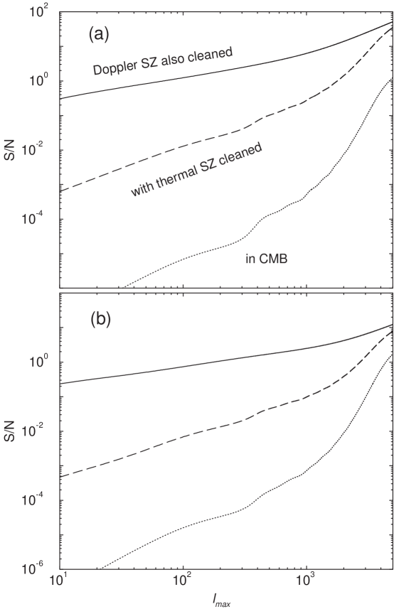
Figure 6.1: Cumulative signal-to-noise for the detection of SZ thermal-SZ thermal-SZ kinetic bispectrum (a) and skewness (b). The dotted line is for the detection of SZ thermal-SZ kinetic correlation using CMB data alone, while the dashed line is the same when the SZ thermal effect has been separated from other CMB contributions and the measurement now involves two points from the SZ map and one point from the CMB. Finally, the solid line is the maximum signal-to-noise for achievable with the separation of the SZ kinetic effect from all contributors to CMB anisotropy.

In order to construct the bispectrum, note that

$$\langle a_{l_{1}m_{1}}^{\rm SZ}a_{l_{2}m_{2}}^{\rm SZ}a_{l_{3}m_{3}}^{\rm kSZ}\rangle=(-1)^{l_{3}}\langle a_{l_{1}m_{1}}^{\rm SZ}a_{l_{2}m_{2}}^{\rm SZ}a_{l_{3}-m_{3}}^{\rm kSZ}\rangle\;.$$ (6.4)

The bispectrum then becomes

$$B_{l_{1}l_{2}l_{3}} = \sum_{m_{1}m_{2}m_{3}}\left(\begin{array}[]{ccc}l_{1}&l_{2}&l_{3}\\ m_{1}&m_{2}&m_{3}\end{array}\right)\Big{(}\langle a^{\rm SZ}_{l_{1}m_{1}}a^{\rm SZ}_{l_{2}m_{2}}a^{\rm kSZ}_{l_{3}m_{3}}\rangle+$$

$$\times\langle a^{\rm SZ}_{l_{2}m_{2}}a^{\rm SZ}_{l_{3}m_{3}}a^{\rm kSZ}_{l_{1}m_{1}}\rangle+\langle a^{\rm SZ}_{l_{3}m_{3}}a^{\rm SZ}_{l_{1}m_{1}}a^{\rm kSZ}_{l_{2}m_{2}}\rangle\Big{)}$$

$$= \sqrt{\frac{(2l_{1}+1)(2l_{2}+1)(2l_{3}+1)}{4\pi}}\left(\begin{array}[]{ccc}l_{1}&l_{2}&l_{3}\\ 0&0&0\end{array}\right)[b^{{\rm S}-{\rm S}}_{l_{1},l_{2}}+{\rm Perm.}]\,,$$ (6.10)

with

$$b^{{\rm SZ}-{\rm SZ}}_{l_{1},l_{2}} = \frac{2^{2}}{\pi^{2}}\int k_{1}^{2}dk_{1}\int k_{2}^{2}dk_{2}P_{\delta\Pi}(k_{1})P_{g\Pi}(k_{2})$$ (6.11)

$$\times I^{\rm kSZ}_{l_{1},l_{2}}(k_{1},k_{2})I_{l_{1}}^{\rm SZ}(k_{1})I_{l_{2}}^{\rm SZ}(k_{2})\,.$$

Note that we have rewritten the $k_{1}\rightarrow k_{2}$ term in Eq. 6.2 as an $l_{1}\rightarrow l_{2}$ interchange so that in Eq. 6.10 “Perm.” means a sum over the remaining 5 permutations of ($l_{1}$,$l_{2}$,$l_{3}$) as usual.

In general, Eq. 6.11 involves five integrations, three over radial distances and two over wavenumbers. These integrals can be simplified using the Limber approximation for sufficiently large $(l_{1},l_{2})$ and we employ the completeness relation of spherical Bessel functions in Eq. 2.27. Applying this to the integral over $k_{2}$ yields

$$b^{{\rm SZ}-{\rm SZ}}_{l_{1},l_{2}}=\frac{2}{\pi}\int\frac{dr}{d_{A}^{2}}W^{\rm SZ}(r)gP_{g\Pi}\left(\frac{l_{2}}{d_{A}};r\right)$$

$$\times \int dr_{1}\int k_{1}dk_{1}P_{\delta\Pi}^{2h}(k_{1};r_{1})W^{\rm SZ}(r_{1})j_{l_{1}}^{\prime}(k_{1}r_{1})j_{l_{1}}(k_{1}r)\,,$$

which we will use to evaluate the SZ thermal-SZ thermal-SZ kinetic bispectrum.

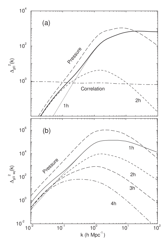
Figure 6.2: The baryon-pressure (a) power spectrum (b) trispectrum today ($z=0$) broken into individual contributions under the halo description. The line labeled ’correlation’ shows the correlation coefficient of gas-pressure correlation with respect to gas-gas and pressure-pressure. For reference, we also show the pressure power spectrum and the trispectrum.

In [Cooray & Hu] (2000), we assumed that pressure traces dark matter to calculate the SZ-SZ-OV bispectrum. Using our halo model, we can now update this calculation to include the bispectrum formed between SZ thermal-SZ thermal-SZ kinetic effects. Additionally, we can investigate the improvements in the signal-to-noise for the bispectrum detections when the SZ thermal effect is separated from CMB. The maximum signal-to-noise for this bispectrum can only be achieved when the SZ kinetic effect is also separated from CMB, though, given that the two effects have the same frequency dependence, it is unlikely that the kinetic SZ effect can be separated from thermal CMB anisotropies. With SZ separated from CMB, however, it is likely that the SZ kinetic effect will dominate the small angular scale signal in the temperature anisotropies. Thus, one can use small angular scale thermal CMB temperature fluctuations for the cross-correlation purposes between thermal SZ and kinetic SZ effects.

In Eq. LABEL:eqn:finalintegral, $P_{g\Pi}$ is the baryon-pressure power spectrum while the $P_{\delta\Pi}$ is the density-pressure power spectrum, with the density field tracing the linear regime of fluctuations. Since there is no contribution coming from the non-linear regime (ie. the 1-halo term), we model this as the large scale density-pressure correlations in the linear regime described by the 2-halo term.

Following [Cooray & Hu] (2000), the signal-to-noise for the detection of the bispectrum is

$$\left(\frac{{\rm S}}{{\rm N}}\right)^{2}\equiv{1\over\sigma^{2}(A)}=\sum_{l_{3}\geq l_{2}\geq l_{1}}\frac{B_{l_{1}l_{2}l_{3}}^{2}}{C_{l_{1}}^{\rm t}C_{l_{2}}^{\rm t}C_{l_{3}}^{\rm t}}\,,$$ (6.13)

where

$$C_{l}^{\rm t}=C_{l}^{\rm CMB}+C_{l}^{\rm sec}+C_{l}^{\rm Noise}\,.$$ (6.14)

In [Cooray et al.] (2000a), we suggested that multifrequency cleaning of SZ effect can be a useful tool for higher order correlation studies and discussed how the signal-to-noise for the detection of SZ-lensing correlation, again through a bispectrum, can be improved by using CMB primary anisotropy separated SZ map. We present the same approach here, where we study the possibility for a detection of the SZ thermal-SZ kinetic correlation by using a frequency cleaned SZ thermal map, which will provide two measurements, and the remainder, which will contain CMB primary, SZ kinetic and other secondary effects and proving a single measurement for the bispectrum.

In Fig. 6.1(a), we update results for the bispectrum given in [Cooray & Hu] (2000), where we only studied the possible detection in CMB data alone and with no consideration for separation of effects, especially the SZ thermal effect. The separation allows a decrease in cosmic variance, as the noise is no longer dominated by CMB primary anisotropies. This leads to an increase in the cumulative signal-to-noise. With SZ thermal effect separated, we see that the signal-to-noise increases by roughly two orders of magnitude. In [Cooray et al.] (2000a), we showed how one can obtain an order of magnitude in signal-to-noise when a CMB separated SZ thermal map is used for a detection of SZ-lensing correlation. Here, we obtain another order of magnitude improvement, since the SZ thermal-SZ kinetic correlation is present with two SZ thermal measurements, instead of one in the case SZ thermal-lensing correlation (in SZ thermal-CMB-CMB bispectrum). Note that one cannot use multifrequency data to separate SZ kinetic from rest of the contributions. Thus, CMB primary anisotropies and other secondary effects still contribute to the variance.

If one can separate the SZ kinetic such that a perfect SZ kinetic map, as well as a perfect SZ thermal map, is available, then one can improve the signal-to-noise for detection significantly such that a detection is possible. Since SZ kinetic is expected to dominate anisotropies at small angular scales, when SZ thermal is removed, an opportunity to detect the SZ thermal-SZ kinetic correlation will likely come from small angular scale multifrequency experiments. One can also improve the possibility of detecting this correlation by noting that the configuration for the bispectrum is such that it peaks for highly flattened triangles (see, [Cooray & Hu] 2000). Thus, in addition to small angular scale experiments, information from large angular scale observations may also be necessary for a detection of this correlation. It is likely that progress in experimental studies will continue to a level where such studies will eventually be possible.

6.2.1 Skewness

Since the bispectrum may be hard to calculate from observational data, we also consider a real space statistic that probes the non-Gaussian information at the three point level. The simplest aspect of the bispectrum that can be measured in real space is the third moment of the map smoothed on some scale with a window $W(\sigma)$

$$\left<\Theta^{3}(\hat{\bf n};\sigma)\right> = {1\over 4\pi}\sum_{l_{1}l_{2}l_{3}}\sqrt{(2l_{1}+1)(2l_{2}+1)(2l_{3}+1)\over 4\pi}$$ (6.17)

$$\times\left(\begin{array}[]{ccc}l_{1}&l_{2}&l_{3}\\ 0&0&0\end{array}\right)B_{l_{1}l_{2}l_{3}}W_{l_{1}}(\sigma)W_{l_{2}}(\sigma)W_{l_{3}}(\sigma)\,,$$

where $W_{l}$ are the multipole moments (or Fourier transform in a flat-sky approximation) of the window. Note that the skewness can then be calculated as $s_{3}=\left<\Theta^{3}(\hat{\bf n};\sigma)\right>/\left<\Theta^{2}(\hat{\bf n};\sigma)\right>^{2}$.

The overall signal-to-noise for the measurement of the third moment is

$$\left({S\over N}\right)^{2}={f_{\rm sky}}{\left<\Theta^{3}(\hat{\bf n};\sigma)\right>^{2}\over{\rm Var}}$$ (6.19)

where the variance, assuming Gaussian statistics, is given by

$${\rm Var} = {1\over(4\pi)^{2}}\sum_{l_{1}l_{2}l_{3}}{(2l_{1}+1)(2l_{2}+1)(2l_{3}+1)\over 4\pi}\left(\begin{array}[]{ccc}l_{1}&l_{2}&l_{3}\\ 0&0&0\end{array}\right)^{2}$$ (6.23)

$$\times W_{l_{1}}^{2}(\sigma)W_{l_{2}}^{2}(\sigma)W_{l_{3}}^{2}(\sigma)6C_{l_{1}}^{\rm t}C_{l_{2}}^{\rm t}C_{l_{3}}^{\rm t}\,.$$

In Fig. 6.1(b), we show the signal to noise for the detection of the third moment. Here, we use a top-hat window in multipole space out to $l_{\rm max}$ so that direct comparison is possible with the signal-to-noise calculation involving the bispectrum. As shown, we find that there is considerably less signal-to-noise in the skewness when compared to the full bispectrum itself. This results from the fact that bispectrum contains all information at the three point level, while with the third moment results in a loss of information. This can also be understood by noting that the signal-to-noise for the bispectrum and skewness is such that in the case of the bispectrum signal-to-noise is calculated for each mode and summed up while for the skewness signal-to-noise is calculated after summing the signal and noise separately over all modes.

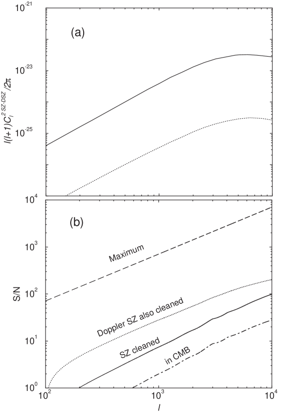
Figure 6.3: (a) The SZ thermal-SZ kinetic power spectrum of squared temperatures. Here, we show the contribution to the power spectrum when only Gaussian terms (dotted line) and when when non-Gaussianities are introduced (solid line). In (b), we show the cumulative signal-to-noise for the detection of the SZ thermal-SZ kinetic squared temperature power spectrum using information in multipoles from 2000 to 10000 and assuming no instrumental or any other noise contributions to the covariance. The signal-to-noise is calculated assuming the power spectrum is measured in CMB data (dot-dashed line), with a perfect frequency cleaned SZ thermal map (solid line) and with a perfect SZ thermal and SZ kinetic effect maps (dotted line).

6.3 The SZ Thermal²-SZ kinetic² Power Spectrum

In addition to the SZ thermal-SZ kinetic-SZ kinetic bispectrum, we can introduce higher order correlations involving the SZ thermal and SZ kinetic effect that probe the correlation between the two. One such a possibility is the trispectrum formed by the SZ thermal and SZ kinetic effect. Given that we do not have a reliable method to measure the bispectrum even, the measurement of such a higher order correlations in experimental data is likely to be challenging.

Here, we focus on a statistic that captures the correlation information coming from higher order, essentially from a trispectrum, but is easily measurable in experimental data since it only involves only a power spectrum. Such a possibility involves the power spectrum of squared temperatures instead of the usual temperature itself. Our motivation for such a statistic came when we inspected the published maps of the large scale SZ thermal and SZ kinetic effects in simulations by [Springel et al.] and realized that there is a significant correlation between the two effects. Since the temperature fluctuations produced by the SZ kinetic effect oscillates between positive and negative values depending on the direction of the velocity field along the line of sight, as stated earlier, a direct two point correlation involving the temperature results in no contribution. A non-zero correlation between the SZ thermal and SZ kinetic effects still manifests if the absolute value of the temperature fluctuation due to kinetic SZ effect is considered. Since absolute value of temperature is equivalent to squaring the temperature, we consider the cross-correlation of SZ thermal and SZ kinetic effects involving the power spectrum of squared temperatures here.

In order to calculate the SZ thermal²-SZ kinetic² power spectrum, we first note that the spherical harmonic coefficient of the squared can be written through a convolution of the spherical moments of the fluctuations

$$a_{lm}^{2} = \int d\hat{\bf n}Y_{l}^{\ast m}T^{2}(\hat{\bf n})$$ (6.24)

$$= \sum_{l_{1}m_{1}}\sum_{l_{2}m_{2}}a_{l_{1}m_{1}}a^{\ast}_{l_{2}m_{2}}\int d\hat{\bf n}Y_{l}^{\ast m}(\hat{\bf n})Y_{l_{1}}^{m_{1}}(\hat{\bf n})Y_{l_{2}}^{\ast m_{2}}(\hat{\bf n})\,,$$

where

$$T(\hat{\bf n})=\sum_{lm}a_{lm}Y_{l}^{\ast m}$$ (6.25)

Note that the integral over three spherical harmonic coefficients can be written through the use of the Gaunt integral.

Using this identity, we can now construct the power spectrum of thermal SZ²-kinetic SZ² as

$$\langle a_{lm}^{{\rm kSZ}^{2}}a_{l^{\prime}m^{\prime}}^{\ast SZ^{2}}\rangle=C_{l}^{2{\rm kSZ}-{\rm SZ}}\delta_{l,l^{\prime}}\delta_{m,m^{\prime}}$$

$$= \sum_{l_{1}m_{1}l_{2}m_{2}}\sum_{l_{3}m_{3}l_{4}m_{4}}\langle a_{l_{1}m_{1}}^{{\rm kSZ}}a_{l_{2}m_{2}}^{\rm kSZ}a_{l_{3}m_{3}}^{\ast SZ}a_{l_{4}m_{4}}^{SZ}\rangle^{\rm t}$$

$$\times \int d\hat{\bf n}Y_{l}^{\ast m}(\hat{\bf n})Y_{l_{1}}^{m_{1}}(\hat{\bf n})Y_{l_{2}}^{\ast m_{2}}(\hat{\bf n})\int d\hat{\bf m}Y_{l^{\prime}}^{m^{\prime}}(\hat{\bf m})Y_{l_{3}}^{\ast m_{3}}(\hat{\bf m})Y_{l_{4}}^{m_{4}}(\hat{\bf m})\,,$$

involving two cumulants of the SZ thermal and SZ kinetic effect, respectively.

After the multipole moments of the SZ effect in Eq. 6.1 and the kinetic SZ effect from Eq. 5.5, we can write the cumulant involving the four moments as

$$\langle a_{l_{1}m_{1}}^{\rm kSZ}a_{l_{2}m_{2}}^{\rm kSZ}a_{l_{3}m_{3}}^{\ast SZ}a_{l_{4}m_{4}}^{SZ}\rangle$$

$$= \frac{(4\pi)^{8}}{9}\int dr_{1}...\int dr_{4}\int{d^{3}{\bf k_{1}}\over(2\pi)^{3}}...\int{d^{3}{\bf k_{6}}\over(2\pi)^{3}}\sum_{l_{1}^{\prime}m_{1}^{\prime}l_{1}^{\prime\prime}m_{1}^{\prime\prime}m_{1}^{\prime\prime\prime}}\sum_{l_{2}^{\prime}m_{2}^{\prime}l_{2}^{\prime\prime}m_{2}^{\prime\prime}m_{2}^{\prime\prime\prime}}i^{l_{1}^{\prime}+l_{1}^{\prime\prime}+l_{4}}(-i)^{l_{2}^{\prime}+l_{2}^{\prime\prime}+l_{3}}$$

$$\times (g\dot{G}G)_{r_{1}}(g\dot{G}G)_{r_{2}}W^{\rm sz}(r_{3})W^{\rm sz}(r_{4})\langle\delta_{\delta}({\bf k_{1}})\delta_{g}({\bf k_{2}})\delta_{\delta}({\bf k_{3}})\delta_{g}({\bf k_{4}})\delta_{\Pi}({\bf k_{5}})\delta_{\Pi}({\bf k_{6}})\rangle$$

$$\times \frac{j_{l_{1}^{\prime}}(k_{1}r_{1})}{k_{1}}j_{l_{1}^{\prime\prime}}(k_{2}r_{1})\frac{j_{l_{2}^{\prime}}(k_{3}r_{2})}{k_{3}}j_{l_{2}^{\prime\prime}}(k_{4}r_{2})j_{l_{3}}(k_{5}r_{3})j_{l_{4}}(k_{6}r_{4})$$

$$\times Y_{l_{1}^{\prime}}^{m_{1}^{\prime}}(\hat{{\bf k}}_{1})Y_{1}^{m_{1}^{\prime\prime\prime}}(\hat{{\bf k}}_{1})Y_{l_{1}^{\prime\prime}}^{m_{1}^{\prime\prime}}(\hat{{\bf k}}_{2})Y_{l_{2}^{\prime}}^{m_{2}^{\prime}}(\hat{{\bf k}}_{3})Y_{1}^{m_{2}^{\prime\prime\prime}}(\hat{{\bf k}}_{3})Y_{l_{2}^{\prime\prime}}^{m_{2}^{\prime\prime}}(\hat{{\bf k}}_{4})Y_{l_{3}}^{m_{3}}(\hat{{\bf k}}_{5})Y_{l_{4}}^{m_{4}}(\hat{{\bf k}}_{6})$$

$$\times \int d\hat{\bf n}Y_{l_{1}}^{m_{1}\ast}(\hat{\bf n})Y_{l_{1}^{\prime}}^{m_{1}^{\prime}\ast}(\hat{\bf n})Y_{l_{1}^{\prime\prime}}^{m_{1}^{\prime\prime}\ast}(\hat{\bf n})Y_{1}^{m_{1}^{\prime\prime\prime}\ast}(\hat{\bf n})$$

$$\times \int d\hat{\bf m}Y_{l_{2}}^{m_{2}\ast}(\hat{\bf m})Y_{l_{2}^{\prime}}^{m_{2}^{\prime}\ast}(\hat{\bf m})Y_{l_{2}^{\prime\prime}}^{m_{2}^{\prime\prime}\ast}(\hat{\bf m})Y_{1}^{m_{2}^{\prime\prime\prime}\ast}(\hat{\bf m})\,.$$

The cumulant involving six density, baryon and pressure fluctuations can be broken in to two parts involving a Gaussian term, with contributions coming from power spectra of velocities and pressure-density correlations, and a non-Gaussian term, with the velocity power spectrum and the pressure-pressure-baryon-baryon trispectrum. Here, we ignore the correlations between pressure and velocity or between baryons and velocities as the scales for such correlations do not match, especially in the small angular scale of interest here. Thus, we write

$$\langle\delta_{\delta}({\bf k_{1}})\delta_{g}({\bf k_{2}})\delta_{\delta}({\bf k_{3}})\delta_{g}({\bf k_{4}})\delta_{\Pi}({\bf k_{5}})\delta_{\Pi}({\bf k_{6}})\rangle$$

$$= \langle\delta_{\delta}({\bf k_{1}})\delta_{\delta}({\bf k_{3}})\rangle\langle\delta_{g}({\bf k_{2}})\delta_{\Pi}({\bf k_{5}})\rangle\langle\delta_{g}({\bf k_{4}})\delta_{\Pi}({\bf k_{6}})\rangle$$

$$+ \langle\delta_{\delta}({\bf k_{1}})\delta_{\delta}({\bf k_{3}})\rangle\langle\delta_{g}({\bf k_{2}})\delta_{\Pi}({\bf k_{5}})\delta_{g}({\bf k_{4}})\delta_{\Pi}({\bf k_{6}})\rangle\,.$$

We first discuss the Gaussian piece given in the first line above. This term, and a permutation, contributes to the cross-correlation and involves the linear density field power spectrum and the non-linear cross-correlation between baryon and pressure fields. Keeping track of the permutation, and after several simplifications, we write

$$\langle a_{l_{1}m_{1}}^{\rm kSZ}a_{l_{2}m_{2}}^{\rm kSZ}a_{l_{3}m_{3}}^{\ast SZ}a_{l_{4}m_{4}}^{SZ}\rangle^{\rm G}$$

$$= \frac{(4\pi)^{8}}{9}\int dr_{1}...\int dr_{4}\int{d^{3}{\bf k_{1}}\over(2\pi)^{3}}\int{d^{3}{\bf k_{2}}\over(2\pi)^{3}}\int{d^{3}{\bf k_{4}}\over(2\pi)^{3}}\sum_{l_{1}^{\prime}m_{1}^{\prime}m_{1}^{\prime\prime\prime}}\sum_{l_{2}^{\prime}m_{2}^{\prime}m_{2}^{\prime\prime\prime}}i^{l_{1}^{\prime}+l_{3}+l_{4}}(-i)^{l_{2}^{\prime}+l_{3}+l_{4}}$$

$$\times (g\dot{G}G)_{r_{1}}(g\dot{G}G)_{r_{2}}W^{\rm sz}(r_{3})W^{\rm sz}(r_{4})P_{\delta\delta}^{\rm lin}(k_{1})P_{g\Pi}(k_{2})P_{g\Pi}(k_{4})$$

$$\times \frac{j_{l_{1}^{\prime}}(k_{1}r_{1})}{k_{1}}j_{l_{3}}(k_{2}r_{1})\frac{j_{l_{2}^{\prime}}(k_{1}r_{2})}{k_{1}}j_{l_{4}}(k_{4}r_{2})j_{l_{3}}(k_{2}r_{3})j_{l_{4}}(k_{4}r_{4})$$

$$\times Y_{l_{1}^{\prime}}^{m_{1}^{\prime}}(\hat{{\bf k}}_{1})Y_{1}^{m_{1}^{\prime\prime\prime}}(\hat{{\bf k}}_{1})Y_{l_{2}^{\prime}}^{m_{2}^{\prime}}(\hat{{\bf k}}_{1})Y_{1}^{m_{2}^{\prime\prime\prime}}(\hat{{\bf k}}_{1})$$

$$\times \int d\hat{\bf n}Y_{l_{1}}^{m_{1}\ast}(\hat{\bf n})Y_{l_{1}^{\prime}}^{m_{1}^{\prime}\ast}(\hat{\bf n})Y_{l_{3}}^{m_{3}\ast}(\hat{\bf n})Y_{1}^{m_{1}^{\prime\prime\prime}\ast}(\hat{\bf n})$$

$$\times \int d\hat{\bf m}Y_{l_{2}}^{m_{2}\ast}(\hat{\bf m})Y_{l_{2}^{\prime}}^{m_{2}^{\prime}\ast}(\hat{\bf m})Y_{l_{4}}^{m_{4}\ast}(\hat{\bf m})Y_{1}^{m_{2}^{\prime\prime\prime}\ast}(\hat{\bf m})\,.$$

Following our derivation of the kinetic SZ power spectrum, we can simplify to obtain

$$\langle a_{l_{1}m_{1}}^{\rm kSZ}a_{l_{2}m_{2}}^{\rm kSZ}a_{l_{3}m_{3}}^{\ast SZ}a_{l_{4}m_{4}}^{SZ}\rangle^{\rm G}=\frac{2^{3}}{\pi^{3}}\int dr_{1}...\int dr_{4}\int k_{1}^{2}dk_{1}\int k_{2}^{2}dk_{2}\int k_{4}^{2}dk_{4}$$

$$\times \sum_{l_{1}^{\prime}}(g\dot{G}G)_{r_{1}}(g\dot{G}G)_{r_{2}}W^{\rm sz}(r_{3})W^{\rm sz}(r_{4})P_{\delta\delta}^{\rm lin}(k_{1})P_{g\Pi}(k_{2})P_{g\Pi}(k_{4})$$

$$\times \frac{j_{l_{1}^{\prime}}^{\prime}(k_{1}r_{1})}{k_{1}}j_{l_{3}}(k_{2}r_{1})\frac{j_{l_{1}^{\prime}}^{\prime}(k_{1}r_{2})}{k_{1}}j_{l_{4}}(k_{4}r_{2})j_{l_{3}}(k_{2}r_{3})j_{l_{4}}(k_{4}r_{4})$$

$$\times \int d\hat{\bf n}Y_{l_{1}}^{m_{1}\ast}(\hat{\bf n})Y_{l_{1}^{\prime}}^{m_{1}^{\prime}\ast}(\hat{\bf n})Y_{l_{3}}^{m_{3}\ast}(\hat{\bf n})\int d\hat{\bf m}Y_{l_{2}}^{m_{2}\ast}(\hat{\bf m})Y_{l_{1}^{\prime}}^{m_{1}^{\prime}\ast}(\hat{\bf m})Y_{l_{4}}^{m_{4}\ast}(\hat{\bf m})\,.$$

Finally, collecting all terms, we write the Gaussian piece of the cross-correlation power between the squared temperatures between thermal SZ and kinetic SZ as

$$\langle a_{lm}^{{\rm kSZ}^{2}}a_{l^{\prime}m^{\prime}}^{\ast SZ^{2}}\rangle^{\rm G}=C_{l}^{\rm G}\delta_{l,l^{\prime}}\delta{m,m^{\prime}}$$

$$= \sum_{l_{1}m_{1}l_{2}m_{2}}\sum_{l_{3}m_{3}l_{4}m_{4}}\sum_{l_{1}^{\prime}}\frac{2^{3}}{\pi^{3}}\int dr_{1}...\int dr_{4}\int k_{1}^{2}dk_{1}\int k_{2}^{2}dk_{2}\int k_{4}^{2}dk_{4}$$

$$\times (g\dot{G}G)_{r_{1}}(g\dot{G}G)_{r_{2}}W^{\rm sz}(r_{3})W^{\rm sz}(r_{4})P_{\delta\delta}^{\rm lin}(k_{1})P_{g\Pi}(k_{2})P_{g\Pi}(k_{4})$$

$$\times \frac{j_{l_{1}^{\prime}}^{\prime}(k_{1}r_{1})}{k_{1}}j_{l_{3}}(k_{2}r_{1})\frac{j_{l_{1}^{\prime}}^{\prime}(k_{1}r_{2})}{k_{1}}j_{l_{4}}(k_{4}r_{2})j_{l_{3}}(k_{2}r_{3})j_{l_{4}}(k_{4}r_{4})$$

$$\times \int d\hat{\bf n}Y_{l_{1}}^{m_{1}\ast}(\hat{\bf n})Y_{l_{1}^{\prime}}^{m_{1}^{\prime}\ast}(\hat{\bf n})Y_{l_{3}}^{m_{3}\ast}(\hat{\bf n})\int d\hat{\bf m}Y_{l_{2}}^{m_{2}\ast}(\hat{\bf m})Y_{l_{1}^{\prime}}^{m_{1}^{\prime}\ast}(\hat{\bf m})Y_{l_{4}}^{m_{4}\ast}(\hat{\bf m})$$

$$\times \int d\hat{\bf n}Y_{l}^{\ast m}(\hat{\bf n})Y_{l_{1}}^{m_{1}}(\hat{\bf n})Y_{l_{2}}^{\ast m_{2}}(\hat{\bf n})\int d\hat{\bf m}Y_{l^{\prime}}^{m^{\prime}}(\hat{\bf m})Y_{l_{3}}^{\ast m_{3}}(\hat{\bf m})Y_{l_{4}}^{m_{4}}(\hat{\bf m})\,.$$

The last four integrals lead to a term that is

$$\sum_{m_{1}m_{2}m_{3}m_{4}}\left(\begin{array}[]{ccc}l_{1}&l_{1}^{\prime}&l_{3}\\ m_{1}&m_{1}^{\prime}&m_{3}\end{array}\right)\left(\begin{array}[]{ccc}l_{2}&l_{1}^{\prime}&l_{4}\\ m_{2}&m_{1}^{\prime}&m_{4}\end{array}\right)\left(\begin{array}[]{ccc}l&l_{1}&l_{2}\\ m&m_{1}&m_{2}\end{array}\right)$$ (6.38)

$$\left(\begin{array}[]{ccc}l^{\prime}&l_{3}&l_{4}\\ m^{\prime}&m_{3}&m_{4}\end{array}\right)=\frac{\delta_{ll^{\prime}}\delta_{mm^{\prime}}}{2l+1}\left\{\begin{array}[]{ccc}l_{4}&l_{2}&l\\ l_{1}&l_{3}&l_{1}^{\prime}\end{array}\right\}$$ (6.43)

Thus, simplifying we obtain

$$C_{l}^{\rm G}=\sum_{l_{1}l_{2}l_{3}l_{4}l_{1}^{\prime}}\frac{\prod_{i=1}^{4}(2l_{i}+1)(2l_{1}^{\prime}+1)}{4\pi}$$

$$\times \left(\begin{array}[]{ccc}l_{1}&l_{1}^{\prime}&l_{3}\\ 0&0&0\end{array}\right)\left(\begin{array}[]{ccc}l_{2}&l_{1}^{\prime}&l_{4}\\ 0&0&0\end{array}\right)\left(\begin{array}[]{ccc}l&l_{1}&l_{2}\\ 0&0&0\end{array}\right)\left(\begin{array}[]{ccc}l&l_{3}&l_{4}\\ 0&0&0\end{array}\right)\left\{\begin{array}[]{ccc}l_{4}&l_{2}&l\\ l_{1}&l_{3}&l_{1}^{\prime}\end{array}\right\}$$

$$\times \frac{2^{3}}{\pi^{3}}\int dr_{1}...\int dr_{4}\int k_{1}^{2}dk_{1}\int k_{2}^{2}dk_{2}\int k_{4}^{2}dk_{4}$$

$$\times (g\dot{G}G)_{r_{1}}(g\dot{G}G)_{r_{2}}W^{\rm sz}(r_{3})W^{\rm sz}(r_{4})P_{\delta\delta}^{\rm lin}(k_{1})P_{g\Pi}(k_{2})P_{g\Pi}(k_{4})$$

$$\times \frac{j_{l_{1}^{\prime}}^{\prime}(k_{1}r_{1})}{k_{1}}j_{l_{3}}(k_{2}r_{1})\frac{j_{l_{1}^{\prime}}^{\prime}(k_{1}r_{2})}{k_{1}}j_{l_{4}}(k_{4}r_{2})j_{l_{3}}(k_{2}r_{3})j_{l_{4}}(k_{4}r_{4})\,.$$

Note that there is an additional term, due to a permutation, which involves by interchanging $l_{3}$ and $l_{4}$ (with $l_{1}^{\prime}$).

Similar to the Limber approximation used with the derivation of the kinetic SZ power spectrum, we can integrate over Bessel functions and simplify to obtain

$$C_{l}^{\rm G}=\sum_{l_{1}l_{2}l_{3}l_{4}l_{1}^{\prime}}\frac{\prod_{i=1}^{4}(2l_{i}+1)(2l_{1}^{\prime}+1)}{4\pi}$$

$$\times \left(\begin{array}[]{ccc}l_{1}&l_{1}^{\prime}&l_{3}\\ 0&0&0\end{array}\right)\left(\begin{array}[]{ccc}l_{2}&l_{1}^{\prime}&l_{4}\\ 0&0&0\end{array}\right)\left(\begin{array}[]{ccc}l&l_{1}&l_{2}\\ 0&0&0\end{array}\right)\left(\begin{array}[]{ccc}l&l_{3}&l_{4}\\ 0&0&0\end{array}\right)\left\{\begin{array}[]{ccc}l_{4}&l_{2}&l\\ l_{1}&l_{3}&l_{1}^{\prime}\end{array}\right\}$$

$$\times \frac{2}{\pi}\int\frac{dr_{1}}{d_{A}^{2}}\int\frac{dr_{2}}{d_{A}^{2}}\int k_{1}^{2}dk_{1}(g\dot{G})_{r_{1}}(g\dot{G})_{r_{2}}W^{\rm sz}(r_{1})W^{\rm sz}(r_{2})$$

$$\times P_{\delta\delta}^{\rm lin}(k_{1})P_{g\Pi}\left(\frac{l_{3}}{d_{A}};r_{1}\right)P_{g\Pi}\left(\frac{l_{4}}{d_{A}};r_{2}\right)\frac{j_{l_{1}^{\prime}}^{\prime}(k_{1}r_{1})}{k_{1}}\frac{j_{l_{1}^{\prime}}^{\prime}(k_{1}r_{2})}{k_{1}}\,.$$

The non-Gaussian piece takes a similar form. After introducing the trispectrum of pressure-pressure-baryon-baryon fluctuations and the power spectrum of velocity correlations, we write

$$\langle a_{l_{1}m_{1}}^{\rm kSZ}a_{l_{2}m_{2}}^{\rm kSZ}a_{l_{3}m_{3}}^{\ast SZ}a_{l_{4}m_{4}}^{SZ}\rangle^{\rm NG}=\frac{(4\pi)^{8}}{9}\int dr_{1}...\int dr_{4}$$

$$\times \int{d^{3}{\bf k_{1}}\over(2\pi)^{3}}\int{d^{3}{\bf k_{2}}\over(2\pi)^{3}}\int{d^{3}{\bf k_{4}}\over(2\pi)^{3}}\int{d^{3}{\bf k_{5}}\over(2\pi)^{3}}\int{d^{3}{\bf k_{6}}\over(2\pi)^{3}}$$

$$\times \sum_{l_{1}^{\prime}m_{1}^{\prime}l_{1}^{\prime\prime}m_{1}^{\prime\prime}m_{1}^{\prime\prime\prime}}\sum_{l_{2}^{\prime}m_{2}^{\prime}l_{2}^{\prime\prime}m_{2}^{\prime\prime}m_{2}^{\prime\prime\prime}}i^{l_{1}^{\prime}+l_{3}+l_{4}}(-i)^{l_{2}^{\prime}+l_{3}+l_{4}}(g\dot{G}G)_{r_{1}}(g\dot{G}G)_{r_{2}}W^{\rm sz}(r_{3})W^{\rm sz}(r_{4})$$

$$\times P_{\delta\delta}^{\rm lin}(k_{1})(2\pi)^{3}T_{\Pi g\Pi g}({\bf k}_{2},{\bf k}_{4},{\bf k}_{5},{\bf k}_{6})\delta_{D}({\bf k}_{2}+{\bf k}_{4}+{\bf k}_{5}+{\bf k}_{6})$$

$$\times \frac{j_{l_{1}^{\prime}}(k_{1}r_{1})}{k_{1}}j_{l_{1}^{\prime\prime}}(k_{2}r_{1})\frac{j_{l_{2}^{\prime}}(k_{1}r_{2})}{k_{1}}j_{l_{2}^{\prime\prime}}(k_{4}r_{2})j_{l_{3}}(k_{2}r_{3})j_{l_{4}}(k_{4}r_{4})$$

$$\times Y_{l_{1}^{\prime}}^{m_{1}^{\prime}}(\hat{{\bf k}}_{1})Y_{1}^{m_{1}^{\prime\prime\prime}}(\hat{{\bf k}}_{1})Y_{l_{2}^{\prime}}^{m_{2}^{\prime}}(\hat{{\bf k}}_{1})Y_{1}^{m_{2}^{\prime\prime\prime}}(\hat{{\bf k}}_{1})Y_{l_{1}^{\prime\prime}}^{m_{1}^{\prime\prime}}(\hat{{\bf k}}_{2})Y_{l_{2}^{\prime\prime}}^{m_{2}^{\prime\prime}}(\hat{{\bf k}}_{4})Y_{l_{3}}^{m_{3}}(\hat{{\bf k}}_{5})Y_{l_{4}}^{m_{4}}(\hat{{\bf k}}_{6})$$

$$\times \int d\hat{\bf n}Y_{l_{1}}^{m_{1}\ast}(\hat{\bf n})Y_{l_{1}^{\prime}}^{m_{1}^{\prime}\ast}(\hat{\bf n})Y_{l_{1}^{\prime\prime}}^{m_{1}^{\prime\prime}\ast}(\hat{\bf n})Y_{1}^{m_{1}^{\prime\prime\prime}\ast}(\hat{\bf n})$$

$$\times \int d\hat{\bf m}Y_{l_{2}}^{m_{2}\ast}(\hat{\bf m})Y_{l_{2}^{\prime}}^{m_{2}^{\prime}\ast}(\hat{\bf m})Y_{l_{2}^{\prime\prime}}^{m_{2}^{\prime\prime}\ast}(\hat{\bf m})Y_{1}^{m_{2}^{\prime\prime\prime}\ast}(\hat{\bf m})\,.$$

To simplify, we expand the delta function associated with the trispectrum in to two separate triangular parts:

$$\delta_{D}({\bf k}_{2}+{\bf k}_{4}+{\bf k}_{5}+{\bf k}_{6})$$

$$= \int\frac{d^{3}{\bf k}^{\prime}}{(2\pi)^{3}}(2\pi)^{3}\delta_{D}({\bf k}_{2}+{\bf k}_{4}+{\bf k}^{\prime})\delta_{D}({\bf k}_{5}+{\bf k}_{6}-{\bf k}^{\prime})$$

$$= \int\frac{d^{3}{\bf x}_{1}}{(2\pi)^{3}}e^{i{\bf x}_{1}\cdot\left({\bf k}_{2}+{\bf k}_{4}+{\bf k}^{\prime}\right)}\int\frac{d^{3}{\bf x}_{2}}{(2\pi)^{3}}e^{i{\bf x}_{2}\cdot\left({\bf k}_{5}+{\bf k}_{6}-{\bf k}^{\prime}\right)}\,.$$

The assumption here is that through this vector expansion, the vectorial representation of the quadrilateral formed by the trispectrum can be expressed through a vectorial configuration of two triangles involving two sides and the diagonal, respectively. With this, the trispectrum is expressed to be dependent only on the magnitude of the vectors ${\bf k}_{2},{\bf k}_{4},{\bf k}_{5},{\bf k}_{6}$ and not on their directions. Using the Rayleigh expansion (Eq. 2.8) in above, we simplify to obtain

$$\langle a_{l_{1}m_{1}}^{\rm kSZ}a_{l_{2}m_{2}}^{\rm kSZ}a_{l_{3}m_{3}}^{\ast SZ}a_{l_{4}m_{4}}^{SZ}\rangle^{\rm NG}=\frac{(4\pi)^{14}}{9}\int dr_{1}...\int dr_{4}\sum_{l_{1}^{\prime}m_{1}^{\prime}l_{1}^{\prime\prime}m_{1}^{\prime\prime}m_{1}^{\prime\prime\prime}}\sum_{l_{2}^{\prime}m_{2}^{\prime}l_{2}^{\prime\prime}m_{2}^{\prime\prime}m_{2}^{\prime\prime\prime}}\sum_{LM}$$

$$\times \int{d^{3}{\bf k_{1}}\over(2\pi)^{3}}\int{d^{3}{\bf k_{2}}\over(2\pi)^{3}}\int{d^{3}{\bf k_{4}}\over(2\pi)^{3}}\int{d^{3}{\bf k_{5}}\over(2\pi)^{3}}\int{d^{3}{\bf k_{6}}\over(2\pi)^{3}}\int{d^{3}{\bf k^{\prime}}\over(2\pi)^{3}}$$

$$\times i^{l_{1}^{\prime}+l_{3}+l_{4}+L}(-i)^{l_{2}^{\prime}+l_{3}+l_{4}-L}i^{l_{1}^{\prime\prime}+l_{2}^{\prime\prime}+l_{3}+l_{4}}$$

$$\times (g\dot{G}G)_{r_{1}}(g\dot{G}G)_{r_{2}}W^{\rm sz}(r_{3})W^{\rm sz}(r_{4})P_{\delta\delta}^{\rm lin}(k_{1})T_{\Pi g\Pi g}(k_{2},k_{4},k_{5},k_{6})$$

$$\times \frac{j_{l_{1}^{\prime}}(k_{1}r_{1})}{k_{1}}j_{l_{1}^{\prime\prime}}(k_{2}r_{1})\frac{j_{l_{2}^{\prime}}(k_{1}r_{2})}{k_{1}}j_{l_{2}^{\prime\prime}}(k_{4}r_{2})j_{l_{3}}(k_{2}r_{3})j_{l_{4}}(k_{4}r_{4})$$

$$\times \int x_{1}^{2}dx_{1}j_{l_{1}^{\prime\prime}}(k_{2}x_{1})j_{l_{2}^{\prime\prime}}(k_{4}x_{1})j_{L}(k^{\prime}x_{1})\int x_{2}^{2}dx_{2}j_{l_{3}}(k_{5}x_{2})j_{l_{4}}(k_{6}x_{2})j_{L}(k^{\prime}x_{2})$$

$$\times Y_{l_{1}^{\prime}}^{m_{1}^{\prime}}(\hat{{\bf k}}_{1})Y_{1}^{m_{1}^{\prime\prime\prime}}(\hat{{\bf k}}_{1})Y_{l_{2}^{\prime}}^{m_{2}^{\prime}}(\hat{{\bf k}}_{1})Y_{1}^{m_{2}^{\prime\prime\prime}}(\hat{{\bf k}}_{1})$$

$$\times \int d\hat{\bf x_{1}}Y_{l_{1}^{\prime\prime}}^{m_{1}^{\prime\prime}}(\hat{\bf x_{1}})Y_{l_{2}^{\prime\prime}}^{m_{2}^{\prime\prime}}(\hat{\bf x_{1}})Y_{L}^{M}(\hat{\bf x_{1}})\int d\hat{\bf x_{2}}Y_{l_{1}^{\prime\prime}}^{m_{1}^{\prime\prime}}(\hat{\bf x_{2}})Y_{l_{2}^{\prime\prime}}^{m_{2}^{\prime\prime}}(\hat{\bf x_{2}})Y_{L}^{M}(\hat{\bf x_{2}})$$

$$\times \int d\hat{\bf n}Y_{l_{1}}^{m_{1}\ast}(\hat{\bf n})Y_{l_{1}^{\prime}}^{m_{1}^{\prime}\ast}(\hat{\bf n})Y_{l_{1}^{\prime\prime}}^{m_{1}^{\prime\prime}\ast}(\hat{\bf n})Y_{1}^{m_{1}^{\prime\prime\prime}\ast}(\hat{\bf n})$$

$$\times \int d\hat{\bf m}Y_{l_{2}}^{m_{2}\ast}(\hat{\bf m})Y_{l_{2}^{\prime}}^{m_{2}^{\prime}\ast}(\hat{\bf m})Y_{l_{2}^{\prime\prime}}^{m_{2}^{\prime\prime}\ast}(\hat{\bf m})Y_{1}^{m_{2}^{\prime\prime\prime}\ast}(\hat{\bf m})\,.$$

Following our derivation of the kinetic SZ power spectrum, and employing the Limber approximation on the Bessel functions, we can simplify further and write the non-Gaussian piece of the correlation between the squared temperatures of SZ thermal and SZ kinetic effects as

$$\langle a_{lm}^{{\rm kSZ}^{2}}a_{l^{\prime}m^{\prime}}^{\ast SZ^{2}}\rangle^{\rm NG}=C_{l}^{\rm NG}\delta_{l,l^{\prime}}\delta{m,m^{\prime}}$$

$$= \frac{2}{\pi}\int\frac{dr}{d_{A}^{6}}\int k_{1}^{2}dk_{1}\sum_{l_{1}^{\prime}m_{1}^{\prime}l_{1}^{\prime\prime}\ m_{1}^{\prime\prime}}\sum_{l_{2}^{\prime\prime}m_{2}^{\prime\prime}LM}\left[(g\dot{G})W^{\rm sz}(r)\right]^{2}$$

$$\times P_{\delta\delta}^{\rm lin}(k_{1})T_{\Pi g\Pi g}\left(\frac{l_{1}^{\prime\prime}}{d_{A}},\frac{l_{2}^{\prime\prime}}{d_{A}},\frac{l_{3}}{d_{A}},\frac{l_{4}}{d_{A}};r\right)\left(\frac{j^{\prime}_{l_{1}^{\prime}}(k_{1}r)}{k_{1}}\right)^{2}$$

$$\times \int d\hat{\bf x_{1}}Y_{l_{1}^{\prime\prime}}^{m_{1}^{\prime\prime}}(\hat{\bf x_{1}})Y_{l_{2}^{\prime\prime}}^{m_{2}^{\prime\prime}}(\hat{\bf x_{1}})Y_{L}^{M}(\hat{\bf x_{1}})\int d\hat{\bf x_{2}}Y_{l_{1}^{\prime\prime}}^{m_{1}^{\prime\prime}}(\hat{\bf x_{2}})Y_{l_{2}^{\prime\prime}}^{m_{2}^{\prime\prime}}(\hat{\bf x_{2}})Y_{L}^{M}(\hat{\bf x_{2}})$$

$$\times \int d\hat{\bf n}Y_{l_{1}}^{m_{1}\ast}(\hat{\bf n})Y_{l_{1}^{\prime}}^{m_{1}^{\prime}\ast}(\hat{\bf n})Y_{l_{1}^{\prime\prime}}^{m_{1}^{\prime\prime}\ast}(\hat{\bf n})\int d\hat{\bf m}Y_{l_{2}}^{m_{2}\ast}(\hat{\bf m})Y_{l_{1}^{\prime}}^{m_{2}^{\prime}\ast}(\hat{\bf m})Y_{l_{2}^{\prime\prime}}^{m_{2}^{\prime\prime}\ast}(\hat{\bf m})$$

$$\times \int d\hat{\bf n}Y_{l}^{\ast m}(\hat{\bf n})Y_{l_{1}}^{m_{1}}(\hat{\bf n})Y_{l_{2}}^{\ast m_{2}}(\hat{\bf n})\int d\hat{\bf m}Y_{l^{\prime}}^{m^{\prime}}(\hat{\bf m})Y_{l_{3}}^{\ast m_{3}}(\hat{\bf m})Y_{l_{4}}^{m_{4}}(\hat{\bf m})\,.$$

Following simplifications used in the case of the Gaussian part, we find

$$C_{l}^{\rm NG}=\sum_{l_{1}l_{2}l_{3}l_{4}l_{1}^{\prime}l_{1}^{\prime\prime}l_{2}^{\prime\prime}}\frac{\prod_{i=1}^{4}(2l_{i}+1)(2l_{1}^{\prime}+1)(2l_{1}^{\prime\prime}+1)(2l_{2}^{\prime\prime}+1)}{(4\pi)^{3}}$$

$$\times \left(\begin{array}[]{ccc}l_{1}&l_{1}^{\prime}&l_{1}^{\prime\prime}\\ 0&0&0\end{array}\right)\left(\begin{array}[]{ccc}l_{2}&l_{1}^{\prime}&l_{2}^{\prime\prime}\\ 0&0&0\end{array}\right)\left(\begin{array}[]{ccc}l&l_{1}&l_{2}\\ 0&0&0\end{array}\right)\left(\begin{array}[]{ccc}l&l_{1}^{\prime\prime}&l_{2}^{\prime\prime}\\ 0&0&0\end{array}\right)\left(\begin{array}[]{ccc}l&l_{3}&l_{4}\\ 0&0&0\end{array}\right)^{2}$$ (6.83)

$$\times \left\{\begin{array}[]{ccc}l_{1}&l_{1}^{\prime}&l\\ l_{2}^{\prime\prime}&l_{1}^{\prime\prime}&l_{2}\end{array}\right\}\frac{2}{\pi}\int\frac{dr}{d_{A}^{6}}\left[(g\dot{G})W^{\rm sz}(r)\right]^{2}$$

$$\times T_{\Pi g\Pi g}\left(\frac{l_{1}^{\prime\prime}}{d_{A}},\frac{l_{2}^{\prime\prime}}{d_{A}},\frac{l_{3}}{d_{A}},\frac{l_{4}}{d_{A}};r\right)\int k_{1}^{2}dk_{1}P_{\delta\delta}^{\rm lin}(k_{1})\left(\frac{j^{\prime}_{l_{1}^{\prime}}(k_{1}r)}{k_{1}}\right)^{2}\,.$$

Note that the total contribution to the thermal SZ²-kinetic SZ² power spectrum is

$$C_{l}^{2{\rm kSZ}-{\rm SZ}}=C_{l}^{\rm G}+C_{l}^{\rm NG}\,.$$ (6.88)

Since the full calculation of the squared power spectra is computationally time consuming, we make several simplifications as outline in the next subsection. These simplifications make use of the fact that at small angular scales, we can utilize flat-sky approximations and that at the same scales, the velocity field is completely independent of the baryon field itself.

6.3.1 Flat-sky approach

Similarly, we can derived the temperature squared power spectrum of kinetic and thermal SZ effects in the flat-sky limit. In the same limit, we also take the velocity field of the kinetic SZ effect to be independent of the baryon fluctuations. Following our previous definitions, we define the flat sky temperature squared power spectrum as

$$\langle\Theta^{2{\rm kSZ}}({\bf l})\Theta^{2{\rm SZ}}({\bf l}^{\prime})\rangle=(2\pi)^{2}\delta_{D}({\bf l}+{\bf l}^{\prime})C_{l}^{2{\rm kSZ}-{\rm SZ}}\,,$$ (6.89)

where the Fourier transform of the squared temperature can be written as a convolution of the temperature transforms

$$\Theta^{2}({\bf l})=\int\frac{d{\bf l}_{1}}{(2\pi)^{2}}\Theta({\bf l}_{1})\Theta({\bf l}-{\bf l}_{1})\,.$$ (6.90)

Here, it should be understood that $\Theta^{2}({\bf l})$ refers to the Fourier transform of the square of the temperature rather than square of the Fourier transform of temperature. We will denote the latter as $[\Theta({\bf l})]^{2}$. To compute the square of the SZ thermal and SZ kinetic temperature power spectrum, we take

$$\langle\Theta^{2{\rm kSZ}}({\bf l})\Theta^{2{\rm SZ}}({\bf l}^{\prime})\rangle=(2\pi)^{2}\delta_{D}({\bf l}+{\bf l}^{\prime})C_{l}$$

$$= \int\frac{d{\bf l}_{1}}{(2\pi)^{2}}\int\frac{d{\bf l}_{2}}{(2\pi)^{2}}\langle\Theta^{\rm kSZ}({\bf l}_{1})\Theta^{\rm kSZ}({\bf l}-{\bf l}_{1})\Theta^{\rm SZ}({\bf l}_{2})\Theta^{\rm SZ}({\bf l}^{\prime}-{\bf l}_{2})\rangle\,.$$

Note that the Fourier transform of the temperature fluctuations in the flat sky is

$$\Theta({\bf l})=\int d^{2}\theta e^{-i{\bf l}\cdot\theta}T(\theta)\,.$$ (6.92)

In the small scale limit where the density field is separated from the velocity field, we can write the above cumulant again in two parts with one involving power spectrum and another with the trispectrum. We first write down the Gaussian-like piece as

$$\langle\Theta^{\rm kSZ}({\bf l}_{1})\Theta^{\rm kSZ}({\bf l}-{\bf l}_{1})\Theta^{\rm SZ}({\bf l}_{2})\Theta^{\rm SZ}({\bf l}^{\prime}-{\bf l}_{2})\rangle^{\rm G}=$$

$$\int\frac{dr_{1}}{d_{A}^{4}}\int\frac{dr_{2}}{d_{A}^{4}}\left[g(r_{1})W^{\rm SZ}(r_{2})\right]^{2}\frac{1}{3}v_{\rm rms}^{2}$$

$$\times \int\frac{dk_{1}}{(2\pi)}\int\frac{dk_{2}}{(2\pi)}e^{ik_{1}r_{1}}e^{ik_{2}r_{2}}\left\langle\delta_{g}\left[\frac{{\bf l}_{1}}{d_{A}},k_{1}\right]\Pi\left[\frac{{\bf l}_{2}}{d_{A}},k_{2}\right]\right\rangle$$

$$\times \int\frac{dk_{3}}{(2\pi)}\int\frac{dk_{4}}{(2\pi)}e^{ik_{3}r_{1}}e^{ik_{4}r_{2}}\left\langle\delta_{g}\left[\frac{{\bf l}-{\bf l}_{1}}{d_{A}},k_{3}\right]\Pi\left[\frac{{\bf l}^{\prime}-{\bf l}_{2}}{d_{A}},k_{4}\right]\right\rangle\,,$$

where we have taken $\langle(\hat{\bf{\theta}}\cdot{\bf v})(\hat{\bf{\theta}}^{\prime}\cdot{\bf v^{\prime}})\rangle\sim 1/3v_{\rm rms}^{2}$ with $1/3$ coming from the fact that only a third of the velocity component contribute to the line of sight rms. We can now introduce the power spectra in above correlators such that

$$\langle\Theta^{\rm kSZ}({\bf l}_{1})\Theta^{\rm kSZ}({\bf l}-{\bf l}_{1})\Theta^{\rm SZ}({\bf l}_{2})\Theta^{\rm SZ}({\bf l}^{\prime}-{\bf l}_{2})\rangle^{\rm G}=$$

$$\int\frac{dr_{1}}{d_{A}^{4}}\int\frac{dr_{2}}{d_{A}^{4}}\left[g(r_{1})W^{\rm SZ}(r_{2})\right]^{2}\frac{1}{3}v_{\rm rms}^{2}$$

$$\times \int\frac{dk_{1}}{(2\pi)}e^{ik_{1}\left(r_{1}-r_{2}\right)}(2\pi)^{2}\delta_{D}\left(\frac{{\bf l}_{1}}{d_{A}}+\frac{{\bf l}_{2}}{d_{A}}\right)P_{g\Pi}\left[\sqrt{\frac{l_{1}^{2}}{r_{1}^{2}}+k_{1}^{2}}\right]$$

$$\times \int\frac{dk_{3}}{(2\pi)}e^{ik_{3}\left(r_{1}-r_{2}\right)}(2\pi)^{2}\delta_{D}\left(\frac{{\bf l}-{\bf l}_{1}}{d_{A}}+\frac{{\bf l}^{\prime}-{\bf l}_{2}}{d_{A}}\right)P_{g\Pi}\left[\sqrt{\frac{|l-l_{1}|^{2}}{r_{1}^{2}}+k_{3}^{2}}\right]\,,$$

and the integrals over the line-of-sight wavevectors behave such that only perpendicular Fourier modes contribute to the projected field, such that $l^{2}/d_{A}^{2}\gg k^{2}$. This is the so-called Limber approximation ([Limber] 1954). Doing the integral over the wavevector, then, results in a delta function in $(r_{1}-r_{2})$ such that only contributions come from the same redshift. Putting the correlator back in the power spectrum equation (Eq. LABEL:eqn:flat), we now get

$$C_{l}^{\rm G}=\int\frac{d^{2}{\bf l}_{1}}{(2\pi)^{2}}\int\frac{dr}{d_{A}^{4}}(g\dot{G})^{2}W^{\rm sz}(r)^{2}2P_{g\Pi}\left(\frac{l_{1}}{d_{A}};r\right)P_{g\Pi}\left(\frac{|{\bf l}-{\bf l}_{1}|}{d_{A}};r\right)\frac{1}{3}v_{\it rms}^{2}\,,$$

where we have introduced a factor of 2 account for the additional permutation involved in the baryon density-pressure correlation.

Similarly, the non-Gaussian piece follows as

$$C_{l}^{\rm NG}=\int\frac{d^{2}{\bf l}_{1}}{(2\pi)^{2}}\int\frac{d^{2}{\bf l}_{2}}{(2\pi)^{2}}\int\frac{dr}{d_{A}^{6}}(g\dot{G})^{2}W^{\rm sz}(r)^{2}\frac{1}{3}v_{\it rms}^{2}$$

$$\times T_{g\Pi g\Pi}\left[\left(\frac{l_{1}}{d_{A}}\right),\left(\frac{|{\bf l}-{\bf l}_{1}|}{d_{A}}\right),\left(\frac{l_{2}}{d_{A}}\right),\left(\frac{|{\bf l}+{\bf l}_{2}|}{d_{A}}\right);r\right]\,.$$

Since we only use the single halo term to calculate $T_{g\Pi g\Pi}$, the arguments are simply scalars and does not dependent on the orientation of the quadrilateral. In general, however, the trispectrum depends on the length of the four sides plus the orientation of at least one of the diagonals.

Comparing the flat sky power spectra written above and the ones derived under the all-sky assumption, we note that the two are related under similar approximations as the ones suggested for comparison between the all-sky and flat-sky kinetic SZ power spectra. For example, for the Gaussian piece, we can obtain the correspondence by setting $l_{1}\sim l_{4}$ and $l_{2}\sim l_{3}$, and further simplifying to separate

$$C_{l}^{\rm G}=\sum_{l_{3}l_{4}}\frac{(2l_{3}+1)(2l_{4}+1)}{4\pi}\left(\begin{array}[]{ccc}l&l_{3}&l_{4}\\ 0&0&0\end{array}\right)^{2}$$

$$\times \int\frac{dr}{d_{A}^{4}}(g\dot{G}G)^{2}W^{\rm sz}(r)^{2}P_{g\Pi}\left(\frac{l_{3}}{d_{A}}\right)P_{g\Pi}\left(\frac{l_{4}}{d_{A}}\right)\frac{1}{3}v_{\it rms}^{2}\,.$$

This requires the sum

$$\sum_{l_{1}l_{2}l_{1}^{\prime}}(2l_{1}+1)(2l_{2}+1)(2l_{1}^{\prime}+1)\left(\begin{array}[]{ccc}l_{1}&l_{1}^{\prime}&l_{2}\\ 0&0&0\end{array}\right)^{2}\left\{\begin{array}[]{ccc}l_{1}&l_{2}&l\\ l_{1}&l_{2}&l_{1}^{\prime}\end{array}\right\}[j^{\prime}_{l_{1}^{\prime}}(kr)]^{2}=\frac{1}{3}\,.$$ (6.105)

We note here that the above relation and the one suggested in Eq. 5.23 agree if we set the index associated with the Bessel function to either $l_{1}$ or $l_{2}$ such that the $l_{1}^{\prime}$ sum reduces to

$$\sum_{l_{1}^{\prime}}(2l_{1}^{\prime}+1)\left\{\begin{array}[]{ccc}l_{1}&l_{2}&l\\ l_{1}&l_{2}&l_{1}^{\prime}\end{array}\right\}=1$$ (6.107)

when $l_{1},l_{2},l$ satisfy the triangular condition. This condition is, in fact, imposed by the Wigner-3$j$ symbol in above.

Finally, the correspondence between the flat sky ${\bf l}$, ${\bf l}_{1}$ and all sky $l,l_{3},l_{4}$ can be noted by introducing ${\bf l}_{3}={\bf l}-{\bf l}_{1}$ and expanding the delta function of $\delta({\bf l}-{\bf l}_{1}-{\bf l}_{3})$ to obtain a Wigner-3$j$ squared symbol in $l,l_{1},l_{3}$ which correspond to $l,l_{3},l_{4}$ in the flat sky formulation. We refer the reader to [Hu] (2000b) for further details in such a reduction. Similarly, we can obtain the correspondence between the flat-sky non-Gaussian expression and the all-sky non-Gaussian expression through a simplification as above for the Wigner-6$j$ symbol. To obtain the correspondence between ${\bf l},{\bf l}_{1},{\bf l}_{2}$ in flat-sky and $l,l_{1},l_{2},l_{3},l_{4}$ we can introduce ${\bf l}_{3}={\bf l}-{\bf l}_{1}$ and ${\bf l}_{4}={\bf l}+{\bf l}_{2}$ to the flat sky expression and break the delta function formed by the flat sky trispectrum involving ${\bf l}_{1}+{\bf l}_{2}+{\bf l}_{3}+{\bf l}_{4}$ to be two parts involving two sides and the diagonal formed by the ${\bf l}$ and expand that as suggested above from [Hu] (2000b). Following simplifications used in the case of the Gaussian part, we find the non-Gaussian piece to be

$$C_{l}^{\rm NG}=\sum_{l_{1}l_{2}l_{3}l_{4}}\frac{\prod_{i=1}^{4}(2l_{i}+1)}{(4\pi)^{2}}\left(\begin{array}[]{ccc}l&l_{1}&l_{2}\\ 0&0&0\end{array}\right)^{2}\left(\begin{array}[]{ccc}l&l_{3}&l_{4}\\ 0&0&0\end{array}\right)^{2}$$

$$\times \int\frac{dr}{d_{A}^{6}}\left[(g\dot{G})W^{\rm sz}(r)\right]^{2}T_{\Pi g\Pi g}\left(\frac{l_{1}^{\prime\prime}}{d_{A}},\frac{l_{2}^{\prime\prime}}{d_{A}},\frac{l_{3}}{d_{A}},\frac{l_{4}}{d_{A}};r\right)\frac{1}{3}v_{\rm rms}^{2}\,.$$

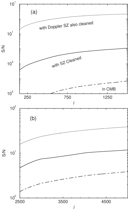
Figure 6.4: The cumulative signal-to-noise for the detection of the thermal SZ-kinetic SZ squared temperature power spectrum. In (a), we consider a large angular scale experiment. The cumulative signal-to-noise, even with a perfectly cleaned SZ map, is significantly less than 1. In (b), we show the cumulative signal-to-noise for a small angular scale experiment; There is now adequate signal-to-noise.

6.3.2 Signal-to-Noise

In order to calculate the possibility for a detection of the thermal SZ²-kinetic SZ² power spectrum, we calculate the signal-to-noise for the detection in couple of experimental possibilities. First, we need to covariance of the estimator involved with the measurement of the squared power spectrum:

$$\hat{C}_{l}^{2{\rm kSZ}-{\rm SZ}}=\frac{A_{f}}{(2\pi)^{2}}\int\frac{d^{2}{\bf l}}{A_{\rm s}}\Theta^{2{\rm kSZ}}({\bf l})\Theta^{2{\rm SZ}}(-{\bf l})\,.$$ (6.114)

Here, $A_{\rm s}=\int d^{2}{\bf l}$ is the area in the two-dimensional shell in Fourier space over which the integral is done and $A_{f}$ is the total area of the survey in Fourier space and can be written as $A_{f}=(2\pi)^{2}/\Omega$ with a total survey area on the sky of $\Omega$. Following [Zaldarriaga] (2000), we can write down the covariance of our estimator as

$${\rm Cov}\left[\left(\hat{C}_{l}^{2{\rm kSZ}-{\rm SZ}}\right)^{2}\right]=\frac{A_{f}}{A_{\rm s}}\left[\left(C_{l}^{2{\rm kSZ}-{\rm SZ}}\right)^{2}+C_{l}^{2{\rm kSZ}-{\rm kSZ}}C_{l}^{2{\rm SZ}-{\rm SZ}}\right]\,,$$

(6.115)

where $C_{l}^{2{\rm kSZ}-{\rm kSZ}}$ is the squared power spectrum of kinetic SZ and thermal SZ while $C_{l}^{2{\rm kSZ}-{\rm kSZ}}$ and $C_{l}^{2{\rm SZ}-{\rm SZ}}$ are the squared power spectra of kinetic SZ and thermal SZ respectively. Here, we assume that squared fields are Gaussian. To calculate $C_{l}^{2{\rm kSZ}-{\rm kSZ}}$ and $C_{l}^{2{\rm SZ}-{\rm SZ}}$ we make several assumptions: We assume that the temperature squared power spectrum will be measured using two maps involving frequency separated SZ contribution (which will have $\Theta^{\rm SZ}+\Theta^{\rm noise}$) and a map with kinetic SZ contribution with the CMB primary component, such that the will be composed of $\Theta^{\rm primary}+\Theta^{\rm kSZ}+\Theta^{{\rm noise}^{\prime}}$. Following such a separation we can write the $C_{l}^{2{\rm SZ}-{\rm SZ}}$ and $C_{l}^{2{\rm kSZ}-{\rm kSZ}}$ as

$$\langle\Theta^{2{\rm SZ}}({\bf l})\Theta^{2{\rm SZ}}({\bf l}^{\prime})\rangle=(2\pi)^{2}\delta_{D}({\bf l}+{\bf l}^{\prime})C_{l}^{2{\rm SZ}-{\rm SZ}}$$

$$= \int\frac{d{\bf l}_{1}}{(2\pi)^{2}}\int\frac{d{\bf l}_{2}}{(2\pi)^{2}}\langle\Theta^{\rm SZ}({\bf l}_{1})\Theta^{\rm SZ}({\bf l}-{\bf l}_{1})\Theta^{\rm SZ}({\bf l}_{2})\Theta^{\rm SZ}({\bf l}^{\prime}-{\bf l}_{2})\rangle\,.$$

$$= \int\frac{d{\bf l}_{1}}{(2\pi)^{2}}\left[2C_{l_{1}}^{\rm SZ}C_{|{\bf l}-{\bf l}_{1}|}^{\rm SZ}+\int\frac{d{\bf l}_{2}}{(2\pi)^{2}}T^{\rm SZ}({\bf l}_{1},{\bf l}-{\bf l}_{1},{\bf l}_{2},-{\bf l}-{\bf l}_{2})\right]\,,$$

where the contributions now come from a Gaussian piece involving the SZ power spectra and a non-Gaussian piece through the SZ trispectrum. Since the primary component fluctuations dominate the kinetic SZ temperature, and that there is no measurable trispectrum for this component under current adiabatic CDM predictions we ignore any non-Gaussian contribution to $C_{l}^{2{\rm kSZ}-{\rm kSZ}}$, and write it as the one with the Gaussian piece in above. This assumption is also safe at small angular scales when $\Theta^{\rm kSZ}>\Theta^{\rm primary}$ since the kinetic SZ effect, under our halo description, is dominated by the large scale correlations and not the single halo term out to $l\sim 10^{4}$.

In the Eq. 6.115, the ratio of $A_{\rm s}/A_{f}$ is the total number of modes that measures the squared power spectrum independently and can be approximated such that $A_{\rm s}/A_{f}=f_{\rm sky}(2l+1)$. To calculate the signal-to-noise involved in the detection of the squared temperature power spectrum, we consider an optimized estimator with weighing factor $W_{l}$ such that

$$\hat{Y}=\sum_{l}W_{l}\hat{C}_{l}^{2{\rm kSZ}-{\rm SZ}}\,,$$ (6.117)

and write the signal-to-noise as

$$\frac{{\rm S}}{{\rm N}}=\left[\frac{\langle\hat{Y}\rangle^{2}}{{\rm Cov}(\hat{Y}^{2})}\right]^{1/2}\,.$$ (6.118)

The weight $W_{l}$ that maximizes the signal-to-noise is $W_{l}=C_{l}^{2{\rm kSZ}-{\rm SZ}}/{\rm Cov}[(C_{l}^{2{\rm kSZ}-{\rm SZ}})^{2}]$ ([Zaldarriaga] 2000) and we can write the required signal-to-noise as

$$\frac{{\rm S}}{{\rm N}}=\left[f_{\rm sky}\sum_{l}(2l+1)\frac{\left(C_{l}^{2{\rm kSZ}-{\rm SZ}}\right)^{2}}{\left(C_{l}^{2{\rm kSZ}-{\rm SZ}}\right)^{2}+C_{l}^{2{\rm kSZ}-{\rm kSZ}}C_{l}^{2{\rm SZ}-{\rm SZ}}}\right]^{1/2}\,.$$

6.4 Discussion

In Fig. 6.3(a), we show the power spectrum of squared temperatures for the SZ thermal and SZ kinetic effects using the halo term. Here, we have separated the Gaussian and non-Gaussian contribution to the squared power spectrum. As shown, the non-Gaussian contribution to the power spectrum is significantly higher than the Gaussian contributions.

The Gaussian contribution to the squared power spectrum traces the pressure-baryon density field power spectrum, which is shown in Fig. 6.2(a) using the halo model. In the same figure, for comparison, we also show the pressure-pressure power spectrum and the correlation coefficient for pressure-baryon with respect to the pressure-pressure and baryon-baryon power spectra. The correlation behaves such that pressure and baryons trace each other at very large scales while the correlation is decreased at small scales due to the turn over in the pressure power spectrum. This is equivalent to the statement that there is no low mass halo contribution to the pressure power spectrum; these halos continue to contribute to the baryon density field power spectrum.

The non-Gaussian contribution to the thermal SZ-kinetic SZ squared temperature power spectrum traces the trispectrum formed by pressure and density field. We show this in Fig. 6.2(b) following the halo model. For comparison, we also show the trispectrum formed by pressure alone in the same figure. The pressure-baryon trispectrum is such that at large scales, corresponding to linear scales, significant contributions come from the correlations between halos instead of the single halo term. If there are significant contributions coming to the squared temperature power spectrum from such linear scales, the Gaussian part of the power spectrum should dominate. Since all contributions to the squared temperature power spectrum comes from small angular scales corresponding to non-linear scales in the pressure-baryon trispectrum, we only use the single halo contribution in calculating the non-Gaussian part of the squared temperature power spectrum. In both Gaussian and non-Gaussian parts of the power spectrum, the velocity field of the halos are taken to be the large scale bulk flows through the linear theory.

In order to assess the maximum possibility for a measurement of the temperature squared power spectrum involving kinetic SZ and thermal SZ, here, we ignore the detector and beam noise contributions to the covariance. Also, we assume full-sky experiments with $f_{\rm sky}=1$.

As written in Eq. LABEL:eqn:conv, the contribution to the covariance comes as a convolution in Fourier space. Thus, even at small angular scales corresponding to high multipoles, noise contributions can come from large angular scales or low wavelength modes. Such modes do not have any signal and by only contributing to the variance, they can reduce the effective signal-to-noise in the measurement. Since the squared power spectrum effectively peaks at multipoles of $\sim$ $10^{4}$, we can essentially ignore any contribution to the signal, as well as noise, from multipoles less than few thousand. These are the same multipoles in which the CMB primary anisotropies dominate, thereby, increasing the effective noise for the measurement. In order to remove the low multipoles, we introduce a filtering scheme to the spherical or Fourier transform of the temperature anisotropy measurements and suppress the low multipole data such that the filter essentially acts as a high pass filter above some $l>l_{\rm min}$.

In Fig. 6.3(b), we show the cumulative signal to noise for the measurement of the thermal SZ-kinetic SZ squared temperature power spectrum. Here, we have assumed an experiment, with no instrumental noise, such that information is only used in multipoles of 2000 to 10000. We find significant signal-to-noise for the detection of the squared temperature power spectrum, especially when using a frequency cleaned SZ map with a CMB map, which has no SZ contribution. One can in fact use the CMB map itself especially if multifrequency information is not available for SZ separation. Since an experiment with multipolar information out to $l\sim 10^{4}$ will not readily be available, we consider two separated realistic cases, involving a large angular scale experiment, similar to Planck, and a small angular scale experiment similar to the ones proposed for the study of SZ effect. We summarize our results in Fig. 6.4. As shown in (a), an experiment only sensitive to multipolar information ranging from 100 to 1500 does not have any signal-to-noise for a detection of the squared power spectrum. With a perfect SZ separated map in this multipolar range, the cumulative signal-to-noise for the squared power spectrum is in the order of $\sim$ 0.01. Thus, it is unlikely that Planck data will be useful for this study. Since we have not included any instrumental noise in calculating signal-to-noise, the realistic signal-to-noise for Planck would be even lower.

Going to smaller angular scales, we find that the signal increases significantly such that an experiment only sensitive to the range of $l\sim 2000$ to 5000 has adequate signal-to-noise for a detection of the squared power spectrum. A multifrequency experiment in the arcminute scales can use its frequency cleaned SZ map to cross-correlate with the CMB map and obtain the squared power spectrum with a cumulative signal-to-noise of order few tens. A comparison to Fig. 6.3(b), suggests that going to lower scales beyond 5000 increases the signal-to-noise, and this is due to the fact that SZ thermal-SZ kinetic squared power spectrum peaks at multipoles of $\sim$ 7000 to 8000, suggesting that for an optimal detection of the squared power spectrum, one should also include observations out to such high multipoles. The increasing activity in the experimental front suggest that such possibilities will soon be available.

Chapter 7 Angular Power Spectrum of Dark Matter Halos as a Cosmological Test

7.1 Introduction

A significant number of observational attempts are now underway to image the large scale structure of the universe out to a redshift of a few. These wide-field surveys involving many tens to thousands of square degrees of angular area on the sky include some of the unique experimental attempts in astronomy: the ongoing Sloan Digital Sky Survey, which measures the distribution of galaxies, the planned weak gravitational lensing shear (see, review by [Bartelmann & Schneider] 2000) observations with dedicated instruments such as the Large Synoptic Survey Telescope (LSST; [Tyson & Angel] 2000) and the Sunyaev-Zel’dovich (SZ; [Sunyaev & Zel’dovich] 1980) effect on the temperature fluctuations of the cosmic microwave background (CMB) at the combined BIMA/OVRO array (CARMA; John Carlstrom, private communication) and with other instruments (e.g., BOLOCAM at CSO; Andrew Lange, private communication). In addition to measurement of properties involved with each of these effects, such as galaxy power spectrum in the case of Sloan or the shear correlations in the case of lensing, these surveys also probe the underlying dark matter distribution of the local universe that define the large scale structure.

Under the context of cold dark matter (CDM) models for structure formation, the dark matter distribution within and between halos has properties that have been intensely studied through analytical techniques and numerical simulations. In particular, analytical descriptions now exist for the abundance (e.g., Press-Schechter mass function; [Press & Schechter] 1974), profile (e.g., Navarro-Frenk-White profile; [Navarro et al] 1996) and correlations of halos of a given mass. Under this halo approach to non-linear clustering, the underlying dark matter distribution of the large scale structure can be described through halos and these halos trace the linear density field power spectrum with a mass and redshift dependent bias given by the halo bias model of [Mo & White] (1996). Using such a halo description, several authors have now shown how to construct the clustering properties of the large scale structure dark matter and other physical properties (e.g., [Seljak] 2000; [Cooray et al] 2000b; [Ma & Fry] 2000a; [Scoccimarro et al.] 2000; [Cooray] 2000).

In [Cooray et al] (2000b), [Cooray & Hu] (2001a) and [Cooray & Hu] (2001b), we studied the statistical properties, mainly the power spectrum, bispectrum and the trispectrum, of weak gravitational lensing convergence of large scale structure through halos. In these papers, we have shown how to construct the statistical measurements of lensing through properties of the dark matter distribution within halos and large scale correlations between halos. The upcoming wide-field weak lensing observations, through galaxy shear data, will essentially measure properties studied in these papers. In addition to statistical properties of weak lensing, the wide-field maps created in the data reduction process is expected to contain additional information such as the spatial distribution of dark matter halos (see, e.g., [Kruse & Schneider] 1999). Similarly, with galaxy imaging data in surveys such as Sloan, one can use the spatial distribution and surface density of galaxies to construct halo catalogs (e.g., [Kepner et al.] 1998).

Thus, it is expected that in wide-field images from current and upcoming surveys, one can identify and produce catalogs of halos responsible for large scale clustering. In fact, with some effects such as the SZ, one should be able to readily identify the halos; in the case of the SZ effect, this is due to fact that large scale pressure power spectrum is mainly due to the massive halos in the universe with highest temperature electrons (see, [Cooray] 2000). Thus, instead of measuring correlation function of the effect itself, one can use the number counts of detected SZ halos as a probe of cosmology (e.g., [Haiman et al.] 2000). In addition to the number counts, important cosmological and astrophysical information can also be obtained through the spatial distribution of halos.

Making an additional use of the spatial distribution of halos in wide-field surveys, we propose the measurement of the comoving angular diameter distance through the angular power spectrum associated with clustering. As in many other classical tests of cosmology, the standard ruler of the proposed test is the shape of the linear power spectrum, which is what will be measured most accurately with upcoming CMB anisotropy observations. With adequate redshift information for halos, such that halo redshift distribution can be binned reliably, we show how one can essentially measure the angular diameter distance to each of the bins through information related to projected linear density power spectrum. Under a cosmological description of the distance, and the evolution of growth, one can determine parameters such as an equation of state for an additional energy density component.

Our proposed cosmological test can be performed easily with upcoming wide-field surveys and will provide an additional use of the data. To a large extent, the method is independent of assumptions such as the mass function which is necessary in many cosmological tests related to number counts. To fully exploit the method, however, a proper understanding of halo bias is needed. Since dark matter halos are involved, necessary information on bias comes directly from N-body simulations. The method can be performed with sources such as galaxies, though, fully understanding galaxy bias can be a problem due to uncertainties associated with galaxy formation etc. Also, since more than one galaxy is present in halos, redshifts for halos can be accurately obtained through photometric techniques than for an individual galaxy. Here, we make the assumption that halo bias is scale independent, though, we will investigate the effect of a scale dependence and suggest that a sharp variation in the halo bias from constant linear value at large scales to a scale-dependent value, say due to the onset of on-linearities, produce a sharp feature in the halo angular power spectrum; such features increase the ability of the halo angular power spectrum as a probe of cosmology. Also, features such as the oscillations due to baryons provide a direct method to calibrate the distance scale independent of other measures of distance. Thus, the technique has the added advantage that it may provide absolute measures of distance.

In the next section, we make predictions for the halo angular power and show that it can be detected in upcoming wide-field surveys. For the illustration of our results, we take a $\Lambda$CDM cosmology with parameters $\Omega_{m}=0.35$ for the matter density, $\Omega_{b}=0.05$ for the baryon density, $\Omega_{\Lambda}=0.65$ for the cosmological constant, $h=0.65$ for the dimensionless Hubble constant, and a scale-invariant spectrum of primordial fluctuations, normalized to galaxy cluster abundances ($\sigma_{8}=0.9$; see, [Viana & Liddle]). For the linear power spectrum, we take the fitting formula for the transfer function given in [Eisenstein & Hu] (1999). We use Press-Schechter (PS; [Press & Schechter] 1974) based theory to define halo redshift distribution. For the illustration of results, we assume a survey of 4000 degrees² with a sensitivity to a minimum halo mass of $10^{14}$ M${}_{\sun}$; The survey area and threshold mass are consistent with planned upcoming lensing and SZ effect surveys (for discussions, see [Kruse & Schneider] 1999; [Holder et al.] 2000; Joffre et al. in preparation).

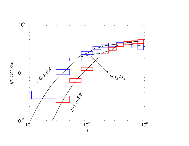
Figure 7.1: Angular power spectrum of halos in a wide-field survey in redshift bins of 0.3 to 0.4 and 1.0 and 1.2. The binned errors assume a survey of 4000 deg², consistent with upcoming weak lensing and SZ surveys. The angular power spectrum at high redshifts is shifted towards the right essentially by the relative change in the comoving angular diameter distance. The oscillations in the angular power spectra are due to baryons in our fiducial cosmological model as calculated numerically with CMBFAST ([Seljak & Zaldarriaga] 1996).

7.2 Angular Power Spectrum

The halo angular power spectrum probes the statistical properties of the halo density field on the sky which is a weighted projection of the matter distribution along the line of sight. We define the angular power spectrum of halos in the flat sky approximation in the usual way

$$\left<n_{h}({\mathbf{l}}_{1})n_{h}({\mathbf{l}}_{2})\right>=(2\pi)^{2}\delta_{\rm D}({\mathbf{l}}_{1}+{\mathbf{l}}_{2})C_{l}\,.$$ (7.1)

Through radial distance projection, we can write (e.g., [Kaiser] 1992)

$$C_{l}=\int dr{W^{2}(r)\over d_{A}^{2}}P_{hh}\left(\frac{l}{d_{A}};r\right)\ \,.$$ (7.2)

Here, $r$ is the comoving radial distance, $d_{A}$ is the comoving angular diameter distance, and $W(r)$ is the normalized radial distribution of the halos. In deriving Eq. 7.2, we have utilized the Limber approximation ([Limber] 1954) by setting $k=l/d_{A}$.

Assuming that halos trace the linear density field, we can write the large scale halo power spectrum as

$$P_{hh}(k;r)=\left<b_{M}\right>^{2}(r)P^{\rm lin}(k;r)$$ (7.3)

where the mass-averaged bias is

$$\left<b_{M}\right>(z)=\frac{1}{\bar{n}_{h}(z)}\int_{M=M_{\rm min}}^{M_{\rm max}}dM\frac{dn(M,z)}{dM}b_{h}(M,z)$$ (7.4)

with the mean number density of halos, as a function of redshift, given by $\bar{n}_{h}(z)=\int dMdn(M,z)/dM$. The halo bias parameters follow from [Mo & White] (1996) and [Mo et al.] (1997):

$$b_{h}(M,z)=1+\frac{\left[\nu^{2}(M,z)-1\right]}{\delta_{c}}\,,$$ (7.5)

where $\nu(M,z)=\delta_{c}/\sigma(M,z)$ is the peak-height threshold. $\sigma(M,z)$ is the rms fluctuation within a top-hat filter at the virial radius corresponding to mass $M$, and $\delta_{c}$ is the threshold overdensity of spherical collapse. Useful fitting functions and additional information on these quantities could be found in [Henry] (2000). The halo mass distribution as a function of redshift $[dn(M,z)/dM]$ is determined through the Press-Schechter (PS; [Press & Schechter] 1974) formalism.

Using bias and the fact that in linear theory the density field is simply scales to higher redshifts through the growth function $G(z)$ where $\delta^{\rm lin}(k;r)=G(r)\delta^{\rm lin}(k;0)$ ([Peebles] 1980), we can write the angular power spectrum of halos between redshift $z_{i}$ and $z_{i}+\Delta z_{i}$ as

$$C_{l}^{i}=\int dzW_{i}(z)^{2}F_{i}(z)P^{\rm lin}\left(\frac{l}{d_{A}^{i}}\right)\,,$$ (7.6)

where the function $F_{i}(z)$, associated with redshift bin $i$, now contains information related to halo bias, growth related to linear evolution, the power spectrum normalization, and terms related to 3-d to 2-d projection (such as a $1/d_{A}^{2}$ term; see, Eq. 7.2).

As written in Eq. 7.6, we can now understand how the halo angular power spectrum allows a determination of the angular diameter distance. Here, $W_{i}(z)$ involves the redshift distribution of halos and this information comes straight from observations while $F_{i}(z)$ contains all other unknowns associated with bias, and thus, the halo mass function, and power spectrum normalization. Our main interest involves the effect of 3-d density field power spectrum and its projection to 2-d angular power spectrum through the Limber form involving $k=l/d_{A}^{i}$. For a given $k$, since $l$ increases as $d_{A}$ is increased, we propose the measurement of angular diameter distance $d_{A}^{i}$ through the relative shift in the halo angular power spectrum in multipole, or Fourier, space.

7.2.1 Theoretical Expectations

In order to discuss the extent to which halos can be used to measure $d_{A}$, we use simple predictions based on the PS description of halo mass function $[dn(M,z)/dM]$. We use the linear mass-averaged bias, $\left<b_{M}\right>(z)$, following the description from [Mo & White] (1996). Since information related to bias is contained within $F_{i}(z)$, its exact value is not important since we construct both the angular diameter distance $d_{A}^{i}$ and $F_{i}(z)$. The exact properties of bias will be necessary, say, if one were to separately study bias from linear evolution of growth. We will later use reasonable priors on bias to estimate errors on $w$, the equation of state of the dark-energy component, using both comoving angular diameter distance and linear evolution of growth.

Following previous studies on the abilities of large structure observations as a probe of cosmology (e.g., [Hu & Tegmark] 1999), we can write the error on the determination of the angular power spectrum of halos as

$$\Delta C_{l}=\sqrt{2\over(2l+1)f_{\rm sky}}\left(C_{l}+C_{l}^{\frac{{\rm S}}{{\rm N}}}\right)\,,$$ (7.7)

where $f_{\rm sky}=\Theta_{\rm deg}^{2}\pi/129600$ is the fraction of the sky covered by a survey of dimension $\Theta_{\rm deg}$ in degrees and $C^{\frac{{\rm S}}{{\rm N}}}$ is the shot-noise power spectrum of halos. Here, we have made the assumption that halo angular power spectrum covariance is described by Gaussian statistics. This is a reasonable assumption to take since we are considering the large scale clustering of halos and that we do not expect non-Gaussianities due to a trispectrum to dominate covariance at such large scales (see, [Cooray & Hu] (2001b) for a discussion of non-Gaussian contribution to the covariance in the case of weak gravitational lensing).

The shot-noise power spectrum is given by the surface-density of halos $C_{l}^{\frac{{\rm S}}{{\rm N}}}\equiv 1/\bar{N}$, which will be available from observations. For calculational purposes here, we again use PS theory to calculate $\bar{N}$

$$\bar{N}=\int dz\frac{d^{2}V}{d\Omega dz}\left[\int dM\frac{dn(M,z)}{dM}\right]\,.$$ (7.8)

Though we calculate the shot-noise term using PS mass function, it is simply the surface density of halos observed in the survey. The shot noise power varies with the mass thresholds detectable in a survey, but in all interesting cases, sets the $l$ at which shot noise from the finite number of halos becomes important. The first term is simply the sampling error assuming Gaussian statistics for the underlying field and makes the fractional errors of order unity at the scale of the survey $l\sim 2\pi/\Theta_{\rm deg}$.

In Fig. 7.1, we illustrate the measurement of the angular diameter distance. The two curves show the halo angular power spectra in two arbitrarily chosen redshift bins of 0.3 to 0.4 and 1.0 to 1.2. The curve corresponding to the higher redshift bin is clearly shifted relative to the one for the lower redshift bin. Note that the oscillatory features corresponding to baryons in our fiducial model is horizontally shifted and this shift simply corresponds to the relative change in the angular diameter distance. In addition to specific features such as oscillations, which may not be easily detectable, one can use the broad feature involving the turnover of the angular halo power spectrum for the purpose of distance determination. Since the scale of baryon oscillations will be known in Mpc^-1 from CMB and will be observed through projection in $h$ Mpc${{}^{-}1}$ with halos, one can use clustering to absolutely calibrate the distance scale through a precise measurement of $h$. Since there may be complications associated with bias and the shot-noise removal, we ignore cosmological information contained in features and only concentrate on the use of overall shape.

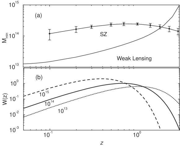
Figure 7.2: (a) The limiting mass for a weak lensing survey (Joffre et al. in preparation) and for a SZ survey ([Holder et al.] 2000). For the purpose of this calculation, we take a constant minimum mass of $10^{14}$ M${}_{\sun}$ out to a redshift of 2. In (b), for reference we show the redshift distribution of halos, as calculated using PS mass function, with minimum masses as noted.

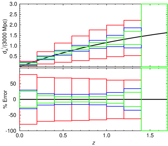
Figure 7.3: (a) The error on angular diameter distance as a function of redshift. We have binned the halos to 9 redshift bins between 0 and 2. The larger errors are with no prior assumption on the cosmological parameters that define the transfer function while the smaller errors are with weak and strong priors (see text). We have taken $l_{\rm max}$ of 1000. In (b), we show relative errors on distance.

7.3 Parameter Estimation

To estimate how well halo clustering can recover certain cosmological and astrophysical parameters, we construct the Fisher matrix:

$${\bf F}_{\alpha\beta}=-\left<\partial^{2}\ln L\over\partial p_{\alpha}\partial p_{\beta}\right>_{\bf x}\,,$$ (7.9)

where $L$ is the likelihood of observing a data set ${\bf x}$ given the true parameters $p_{1}\ldots p_{n}$. With equation (7.7), the Fisher matrix for halo power becomes

$${\bf F}_{\alpha\beta}=\sum_{i=1}^{{\rm N_{\rm bins}}}\sum_{l=l_{\rm min}}^{l_{\rm max}}{f_{\rm sky}(l+1/2)\over(C_{l}^{i}+C_{\frac{{\rm S}}{{\rm N}}}^{i})}{\partial C_{l}^{i}\over\partial p_{\alpha}}{\partial C_{l}^{i}\over\partial p_{\beta}}\,,$$ (7.10)

with the $i$ sum representing the sum over the total number of redshit bins. Since the variance of an unbiased estimator of a parameter $p_{\alpha}$ cannot be less than $({\bf F}^{-1})_{\alpha\alpha}$, the Fisher matrix quantifies the best statistical errors on parameters possible with a given data set.

We choose $l_{\rm min}=2\pi/\Theta_{\rm deg}$ when evaluating equation (7.10) as it corresponds roughly to the survey size. The precise value does not matter for parameter estimation due to the increase in sample variance on the survey scale. We choose a value for $l_{\rm max}$ where $C_{l}^{\frac{{\rm S}}{{\rm N}}}=C_{l}$, which generally ranges from 200 at low redshift bins to 400 at high redshift bins. At low redshifts, this cut off is slightly in the non-linear regime though at redshifts greater than 0.8 or so, one is well within the linear regime. We also use a fix $l_{\rm max}$ of 1000 in all bins, in order to understand the gain in information going to such a high $l$. Using information out to such a high multipole value for cosmological purposes will require a detailed understanding of shot-noise substraction.

Due to the dependence on the linear density field power spectrum, all cosmological parameters that change the shape of the power spectrum across the scales probed by halos also affect the measurement of distance. The shape of the transfer function is determined by $\Omega_{m}h^{2}$ and $\Omega_{b}h^{2}$ while the overall tilt is determined by a scalar tilt $n_{s}$ which we defined to be around a fixed scale. Note that these are the cosmological parameters that will be easily determined from CMB anisotropy observations. When estimating expected errors on distance, we will consider two sets of priors on these cosmological parameters: a prior set consistent with expected errors from MAP missions with $\sigma(\ln\Omega_{m}h^{2})=0.2$ and $\sigma(n_{s})$= 0.11, and a prior set consistent with Planck mission with $\sigma(\ln\Omega_{m}h^{2})=0.064$ and $\sigma(n_{s})$=0.041 (see, [Eisenstein et al.] 2000). In constructing the equation of state for an dark energy, $w$, we make use of the information present in both $d_{A}$ and $G$ by separating $F(z)$ to bias, growth, amplitude of the normalization and information related to radial projection. Since we do not consider information present in baryon oscillations, our predictions for angular diameter distance or associated cosmology is not strongly sensitive to $\Omega_{b}h^{2}$.

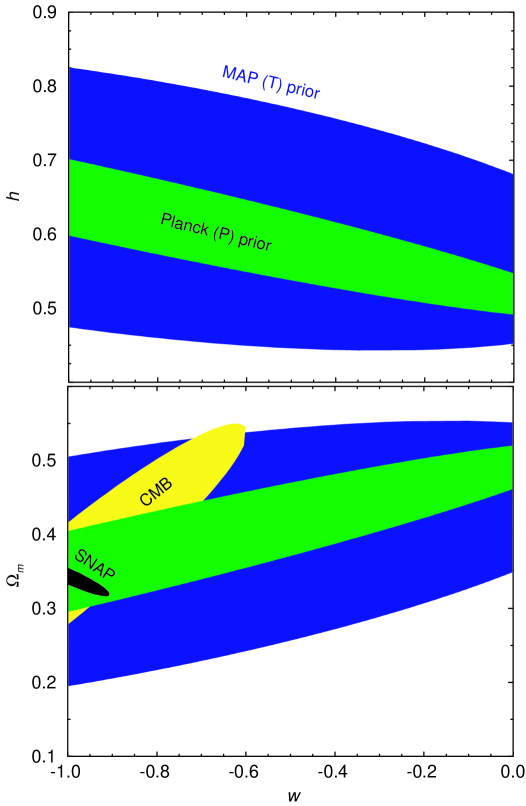
Figure 7.4: (a) The error on parameter $w$, the equation of state for the additional energy density, and $h$ and (b) $w$ and $\Omega_{m}$. We use distance information only. Here, we e show errors for halos with priors following MAP Temp and Planck Temp+Pol.In (b), for reference, we also show errors on $\Omega_{m}$ and $w$ from CMB (involving Planck temperature and polarization) and Type Ia SNe with SNAP mission.

Figure 7.5: The 1-$\sigma$ error on $w$ as a function of the prior on the produce of normalization and bias. The four curves assume Planck (Pol) priors on $\Omega_{m}h^{2}$, $n_{s}$ and $\Omega_{b}h^{2}$ to define the linear power spectrum. The soild line is with no prior on $\ln A$, and $h$. The dotted line includes a prior of 0.2 in $\ln A$, while the long dashed line is with an addition prior of 0.1 in $h$. The dot-dashed line is an highly optimistic scenario with exact $A$, a prior of 0.1 in $h$ and using halo angular power spectrum information out to $l_{\rm max}$ of 1000.

7.4 Results & Discussion

As the first step in distance construction through halo clustering, we consider a non-parametric approach and study the possibility for a measurement of comoving angular diameter distance $d_{A}^{i}$ to each redshift bin $i$. In addition to the distance measurement, we also estimate errors on $F_{i}(z)$, the normalization, which includes details on bias, growth etc. The non-parametric approach to construct $d_{A}^{i}$ is such that it is independent of a particular cosmological model (e.g., open or flat) or the form of the additional energy density at low redshifts, such as a cosmological constant. At each redshift bin, we consider a mean comoving angular diameter distance value valid for that bin $\left<d_{A}^{i}\right>$ and replace this mean value in Eq. 7.6. This mean distance parameter can take any value in each of the bins, independent of its value in adjacent redshift bins. Note that the normalization of the power spectrum, in addition to bias and growth, is included in $F_{i}(z)$ and we do not need to specify them separately here.

In Fig. 7.3(a), we show three sets of errors: the largest errors assume no prior knowledge on the transfer function, while the smaller errors correspond to priors from MAP (Temp) and Planck (Pol) respectively. In Fig. 7.3(b), we show the fractional percentage errors on the distance. The errors in the lowest bins tells us how well one can estimate the Hubble constant, while the slope of $d_{A}(z)$ around $z\sim 1$ provides information on cosmology. Though we have parametrized the distance in each of the redshift bins as an independent quantity, through gloabl parameters such as $\Omega_{m}h^{2}$, the errors on each of these distance estimates are correlated with each at the 5% level.

In a realistic cosmology $d_{A}(z)$ is expected to be sufficiently smooth so as to be adequately parameterized by a small number of parameters at the redshifts in question. Since $\Omega_{m}h^{2}$ is already taken as a parameter, we choose the remaining parameters to be the Hubble constant $H_{0}$ and the equation of state of the dark energy $w$ assuming a flat Universe.

To compare with other cosmological probes we also show the constraints in the $h$-$w$ and $\Omega_{m}$-$w$ plane in Fig. 7.4. The constraints from halos comes directly on the $h$-$w$ plane. As shown in Fig. 7.4(b), note that different linear combinations of $\Omega_{m}$ and $w$ will be determined by halos (which probe $d_{A}$ at $z\sim 1$) and the CMB (which probes $d_{A}$ at $z\sim 1000$), which in the case of CMB is shown for the Planck (with information through polarization also). Although each constraint alone may not be able to pin down $w$, the combined region on $\Omega_{m}$ and $w$ probed by halos and CMB allow very interesting constraints even under our conservative assumptions. We bin halos following the binning scheme in Fig. 7.3, which is somewhar arbitrarily chosen in equal redshift bin sizes at low redshifts. We expect that more information, however, can be gained by optimizing the binning strategies; we relegate these issues to future work.

We now investigate how the relative linear evolution of growth improve constraints on $\Omega_{m}$ and $w$. To obtain interesting constraints, we need to impose the prior on bias, $\left<b_{M}\right>$, and the power spectrum normalization, $A$, separately. In Fig. 7.5, we plot marginalized error on $w$ as a function of the assumed fractional prior on the quantity of $\ln\left<b_{M}\right>$ and for various assumptions with regards to how well we will know $\ln A$ and $h$. Note that the power spectrum normalization, $A$, results in an overall scaling, while the bias, which we parametrize by independent values in each redshift bin, allows for relative variations; Since $A$ affects only an overall scaling and cosmological information from growth comes from relative variations, the effect of an unknown $A$ is minimal. The difference between an unknown $A$ and a prior of 0.2 in $\ln A$ only results in a maximum change of $\sim$ 25% in the error in $w$.

Finally let us address the issue of the scale-dependence of the bias. A scale-dependent bias that can be predicted in fact aids in the determination of angular diameter distances: the scale-dependence acts as another standardizable ruler for the test. Indeed, the scale-dependence of the bias as a function of halo mass is something that can be precisely determined from $N$-body simulations [Kravstov & Klypin] (1999). A more subtle problem is introduced by uncertainties in the mass threshold or selection function. Since the bias is also mass dependent, this translates into uncertainties in the predictions for scale-dependence. To investigate the effects of this sort of uncertainty we can add in an additional parameter and marginalize its effects. We take

$$b_{M}(k,z)=\left<b_{M}\right>(z)\left[1+f\left(\sqrt{\frac{P^{\rm NL}(k;z)}{P^{\rm lin}(k;z)}}-1\right)\right]\,.$$ (7.11)

where $f$ is dimensionless parameter meant to interpolate between the linear and non-linear mass power spectra $P^{\rm NL}$ [Peacock & Dodds] (1996) which has an inflection at the non-linear scale. Under the halo model, a halo power spectrum equal to the non-linear mass power spectrum is the extreme limit since there would then be no room for intrahalo power associated with their profiles. Taking a fiducial model with $f=0$ to be conservative, we find that, in the case with MAP (Temp) priors, error on $w$ increases by less than ten percent from 0.86 to 0.92.

In addition to the scale-dependent bias, the proposed test can be affected by any process that changes the shape of the power spectrum as a function of redshift, e.g. an eV mass neutrino and a running tilt. For neutrinos, while a precise measurement of the linear power spectrum at low redshifts will help resolve any ambiguities, we do not expect a running tilt to be a problem since the decade of scales in the power spectrum probed by CMB is also what is used for the present test.

In spite of these caveats, it is clear that future surveys which can identify dark matter halos as a function of redshift contain valuable information beyond the evolution in their number abundance. As the theoretical modelling of the halo distribution and empirical modelling of the selection process improves, the correlation function of the halos can provide not only the angular diameter distance measures emphasized here but also direct measures of the growth of large-scale structure itself.

Appendix A Trispectrum Under the Halo Model

In this appendix, we discuss the derivation of the trispectrum under the halo model. Even though we limit this discussion to the trispectrum, this derivation can easily be extended to any n-point correlation function in Fourier space. For the purpose of this discussion, we take the approach presented in [Scherrer & Bertschinger] (1991) and write the connected four-point correlation function in real space and take the Fourier transform to construct the trispectrum.

First, we write the dark matter is distribution in halos such that the density at location ${\bf x}$ is $\rho_{h}({\bf x};M)$ and the overdensity as $y({\bf x};M)$. We also take a mass function for halos given by $\frac{d\bar{n}}{dM}$. The Fourier transform of the dark matter distribution within a halo of mass $M$ is

$$\hat{\rho}_{h}({\bf k};M)=\int d^{3}{\bf x}\rho_{h}({\bf x};M)e^{-i{\bf k}\cdot{\bf x}}\,,$$ (A.1)

and we take this to be related to the fourier transform of the overdensity: $y(k,M)=\hat{\rho}_{h}({\bf k};M)/\rho_{b}$, with background mean density of $\rho_{b}$. In addition to dark matter density field, this description applies to any property associated with halos, such as pressure. One has to simply substitute the Fourier transform of the relevant distribution function for $y(k,M)$ for the property of interest. In the rest of the discussion, we will generalize the derivation with an index $i$ in $y_{i}$.

In our simplifications, we will make use of the fact that

$$\delta_{D}({\bf k}_{1234})=\int\frac{d^{3}{\bf x}}{(2\pi)^{3}}e^{-i{\bf x}\cdot({\bf k}_{1}+...+{\bf k}_{4})}\,,$$ (A.2)

where ${\bf k}_{1234}={\bf k}_{1}+{\bf k}_{2}+{\bf k}_{3}+{\bf k}_{4}$.

A fundamental assumption in the halo approach to describe non-linear clustering is that halos themselves are clustered following fluctuations in the linear density field. Using the halo power spectrum, $P_{hh}(k)$, bispectrum, $B_{hhh}({\bf k}_{1},{\bf k}_{2},{\bf k}_{3})$ and trispectrum, $T_{hhhh}({\bf k}_{1},{\bf k}_{2},{\bf k}_{3},{\bf k}_{4})$, we can write the two-point

$$\zeta^{2}_{hh}(M_{1},M_{2};{\bf x}_{1},{\bf x}_{2})=\int\frac{d^{3}{\bf k}^{i}}{(2\pi)^{3}}(2\pi)^{3}P_{hh}(k^{i};M_{1},M_{2})e^{i{\bf k}^{i}\cdot({\bf x}_{1}-{\bf x}_{2})}\,$$ (A.3)

three point

$$\zeta^{3}_{hhh}(M_{1},M_{2},M_{3};{\bf x}_{1},{\bf x}_{2},{\bf x}_{3})=\int\frac{d^{3}{\bf k}^{i}}{(2\pi)^{3}}...\int\frac{d^{3}{\bf k}^{k}}{(2\pi)^{3}}$$

$$B_{hhh}({\bf k}^{i},{\bf k}^{j},{\bf k}^{k};M_{1},M_{2},M_{3})(2\pi)^{3}\delta_{D}({\bf k}_{ijk})e^{i({\bf k}^{i}\cdot{\bf x}_{1}+...+{\bf k}^{k}\cdot{\bf x}_{3})}\,,$$

and four-point

$$\zeta^{4}_{hhhh}(M_{1},M_{2},M_{3},M_{4};{\bf x}_{1},{\bf x}_{2},{\bf x}_{3},{\bf x}_{4})=\int\frac{d^{3}{\bf k}^{i}}{(2\pi)^{3}}...\int\frac{d^{3}{\bf k}^{l}}{(2\pi)^{3}}$$

$$T_{hhhh}({\bf k}^{i},{\bf k}^{j},{\bf k}^{k},{\bf k}^{l};M_{1},M_{2},M_{3},M_{4})(2\pi)^{3}\delta_{D}({\bf k}_{ijkl})e^{i({\bf k}^{i}\cdot{\bf x}_{1}+...+{\bf k}^{l}\cdot{\bf x}_{4})}\,,$$

correlation functions of halos in real space.

Following the arguments presented in § 1.4, we take halos to be clustered following the linear theory, such that the halo power spectrum

$$P_{hh}(k;M_{1},M_{2})=\prod_{i=1}^{2}b_{i}(M_{i})P^{\rm lin}(k)\,,$$ (A.6)

bispectrum

$$B_{hhh}({\bf k}_{1},{\bf k}_{2},{\bf k}_{3};M_{1},M_{2},M_{3})=$$

$$\prod_{i=1}^{3}b_{i}(M_{i})\left[B^{\rm lin}({\bf k}_{1},{\bf k}_{2},{\bf k}_{3})+\frac{b_{2}(M_{3})}{b_{1}(M_{3})}P^{\rm lin}(k_{1})P^{\rm lin}(k_{2})\right]\,,$$

and, trispectrum

$$T_{hhhh}({\bf k}_{1},{\bf k}_{2},{\bf k}_{3},{\bf k}_{4};M_{1},M_{2},M_{3},M_{4})=\prod_{i=1}^{4}b_{i}(M_{i})$$ (A.8)

$$\times \left[T^{\rm lin}({\bf k}_{1},{\bf k}_{2},{\bf k}_{3},{\bf k}_{4})+\frac{b_{2}(M_{4})}{b_{1}(M_{4})}P^{\rm lin}(k_{1})P^{\rm lin}(k_{2})P^{\rm lin}(k_{3})\right]\,,$$

trace the linear theory power spectra and higher order correlations with an $i$th-order bias $b_{i}(M)$ for a halo of mass $M$ relative to the linear dark matter density field. These biases could be found in [Mo et al.] (1997). The linear density field power spectrum comes directly from linear perturbation theory, while the bispectrum and trispectrum requires second-order perturbation theory (see, e.g., [Fry] 1984; [Goroff et al] 1986).

Given a profile, a mass function, and a description of halo clustering, we can now write the four-point correlation functions in real space. We will then consider the Fourier transform of these correlations functions to obtain the trispectrum.

A.0.1 Real Space Four Point Correlation

Following [Scherrer & Bertschinger] (1991), we can separate contributions to the four point correlation function as those arising from one to four halos. Thus,

$$\eta({\bf r}_{1},{\bf r}_{2},{\bf r}_{3},{\bf r}_{4})=\eta^{1h}({\bf r}_{1},{\bf r}_{2},{\bf r}_{3},{\bf r}_{4})+\eta^{2h}({\bf r}_{1},{\bf r}_{2},{\bf r}_{3},{\bf r}_{4})$$ (A.9)

$$+ \eta^{3h}({\bf r}_{1},{\bf r}_{2},{\bf r}_{3},{\bf r}_{4})+\eta^{4h}({\bf r}_{1},{\bf r}_{2},{\bf r}_{3},{\bf r}_{4})\,.$$

Here, ${\bf r}_{i}$ are position vectors from an arbitrary origin. It should be understood that this is the non-Gaussian part of the four point function and that there are no contribution from any Gaussian terms.

The correlation functions involving one to four halos can now be written as integrals over the spatial distribution of the number of halos involved and their mass functions. We first write the four point correlations within a single halo

$$\eta^{1h}({\bf r}_{1},{\bf r}_{2},{\bf r}_{3},{\bf r}_{4})=\int d^{3}{\bf x}_{1}\int dM_{1}\frac{d\bar{n}}{dM_{1}}y_{i}({\bf r}_{1}-{\bf x}_{1};M_{1})...y_{i}({\bf r}_{4}-{\bf x}_{1};M_{1})$$

The two-halo term contains two parts with one involving three point in one halo and the fourth in the second halo and another part with two points in each of the two halos. We write the 3-1 combination first and then the 2-2 combination:

$$\eta^{2h}({\bf r}_{1},{\bf r}_{2},{\bf r}_{3},{\bf r}_{4})=\Big{[}\int d^{3}{\bf x}_{1}\int dM_{1}\frac{d\bar{n}}{dM_{1}}y_{i}({\bf r}_{1}-{\bf x}_{1};M_{1})...y_{i}({\bf r}_{3}-{\bf x}_{1};M_{1})$$ (A.11)

$$\times \int d^{3}{\bf x}_{2}\int dM_{2}\frac{d\bar{n}}{dM_{1}}y_{i}({\bf r}_{4}-{\bf x}_{2};M_{2})$$

$$+ \int d^{3}{\bf x}_{1}\int dM_{1}\frac{d\bar{n}}{dM_{1}}y_{i}({\bf r}_{1}-{\bf x}_{1};M_{1})y_{i}({\bf r}_{2}-{\bf x}_{1};M_{1})\int d^{3}{\bf x}_{2}$$

$$\times \int dM_{2}\frac{d\bar{n}}{dM_{2}}y_{i}({\bf r}_{3}-{\bf x}_{2};M_{2})y_{i}({\bf r}_{4}-{\bf x}_{2};M_{2})\Big{]}\zeta^{2}_{hh}(M_{1},M_{2};{\bf x}_{1},{\bf x}_{2})\,,$$

with $\zeta^{2}_{hh}$ as defined above. Through permutations, the 3 points in one and one point in 2nd term contains a total of four terms while the second part with two point each contains a total of three terms (see, [Scherrer & Bertschinger] 1991).

The three halo term can be written with two points in one halo and a point in each of the other two halos

$$\eta^{3h}({\bf r}_{1},{\bf r}_{2},{\bf r}_{3},{\bf r}_{4})=\int d^{3}{\bf x}_{1}\int dM_{1}\frac{d\bar{n}}{dM_{1}}y_{i}({\bf r}_{1}-{\bf x}_{1};M_{1})y_{i}({\bf r}_{2}-{\bf x}_{1};M_{1})$$ (A.12)

$$\times \int d^{3}{\bf x}_{2}\int dM_{2}\frac{d\bar{n}}{dM_{2}}y_{i}({\bf r}_{3}-{\bf x}_{2};M_{2})\int d^{3}{\bf x}_{3}\int dM_{3}\frac{d\bar{n}}{dM_{3}}y_{i}({\bf r}_{4}-{\bf x}_{3};M_{3})$$

$$\times \zeta^{3}_{hhh}(M_{1},M_{2},M_{3};{\bf x}_{1},{\bf x}_{2},{\bf x}_{3})\,,$$

with the halo three-point correlation function $\zeta^{3}_{hhh}$. Through permutations, with respect to the ordering of ${\bf r}_{1}$ to ${\bf r}_{4}$, there are total of 6 terms involving three halos that contribute to the four point correlations function.

The four halo term involves a point in each of the four halos

$$\eta^{4h}({\bf r}_{1},{\bf r}_{2},{\bf r}_{3},{\bf r}_{4})=\int d^{3}{\bf x}_{1}\int dM_{1}\frac{d\bar{n}}{dM_{1}}y_{i}({\bf r}_{1}-{\bf x}_{1};M_{1})$$

$$\times \int d^{3}{\bf x}_{2}\int dM_{2}\frac{d\bar{n}}{dM_{2}}y_{i}({\bf r}_{3}-{\bf x}_{2};M_{2})\int d^{3}{\bf x}_{3}\int dM_{3}\frac{d\bar{n}}{dM_{3}}y_{i}({\bf r}_{4}-{\bf x}_{3};M_{3})$$

$$\times \int d^{3}{\bf x}_{4}\int dM_{4}\frac{d\bar{n}}{dM_{4}}y_{i}({\bf r}_{4}-{\bf x}_{4};M_{4})\zeta^{4}_{hhhh}(M_{1},M_{2},M_{3},M_{4};{\bf x}_{1},{\bf x}_{2},{\bf x}_{3},{\bf x}_{4})\,,$$

and is proportional to the halo four point correlation function $\zeta^{4}_{hhhh}$.

A.0.2 Trispectrum

In order to derive the dark matter trispectrum using halos, we again break the contributions to four parts involving one to four halos

$$T({\bf k}_{1},{\bf k}_{2},{\bf k}_{3},{\bf k}_{4})=T^{1h}({\bf k}_{1},{\bf k}_{2},{\bf k}_{3},{\bf k}_{4})+T^{2h}({\bf k}_{1},{\bf k}_{2},{\bf k}_{3},{\bf k}_{4})$$ (A.14)

$$+ T^{3h}({\bf k}_{1},{\bf k}_{2},{\bf k}_{3},{\bf k}_{4})+T^{4h}({\bf k}_{1},{\bf k}_{2},{\bf k}_{3},{\bf k}_{4})$$

and define the trispectrum such that

$$\eta({\bf r}_{1},{\bf r}_{2},{\bf r}_{3},{\bf r}_{4})=\int\frac{d^{3}{\bf k}_{1}}{(2\pi)^{3}}...\int\frac{d^{3}{\bf k}_{4}}{(2\pi)^{3}}T({\bf k}_{1},{\bf k}_{2},{\bf k}_{3},{\bf k}_{4})\delta_{D}({\bf k}_{1234})e^{i({\bf k}_{1}\cdot{\bf r}_{1}+...+{\bf k}_{4}\cdot{\bf r}_{4})}\,.$$

We now take the Fourier transform of each of the four terms associated with the real space four-point correlation function.

First, the term involving one halo can be written as

$$\eta^{1h}({\bf r}_{1},{\bf r}_{2},{\bf r}_{3},{\bf r}_{4})=\int\frac{d^{3}{\bf k}_{1}}{(2\pi)^{3}}...\int\frac{d^{3}{\bf k}_{4}}{(2\pi)^{3}}\int dM_{1}\frac{d\bar{n}}{dM_{1}}\hat{y}_{i}({\bf k}_{1};M_{1})...\hat{y}_{i}({\bf k}_{4};M_{1})$$ (A.16)

$$\times e^{i({\bf k}_{1}\cdot{\bf r}_{1}+...+{\bf k}_{4}\cdot{\bf r}_{4})}\int d^{3}{\bf x}_{1}e^{-i{\bf x}_{1}\cdot({\bf k}_{1}+...+{\bf k}_{4})}\,$$

which can be used to write the one-halo contribution to the trispectrum as

$$T^{1h}({\bf k}_{1},{\bf k}_{2},{\bf k}_{3},{\bf k}_{4})=\int dM_{1}\frac{d\bar{n}}{dM_{1}}\hat{y}_{i}({\bf k}_{1};M_{1})...\hat{y}_{i}({\bf k}_{4};M_{1})$$

$$\equiv I^{0}_{4,iiii}(k_{1},k_{2},k_{3},k_{4})$$ (A.17)

Similarly, the term involving two halos is

$$\eta^{2h}({\bf r}_{1},{\bf r}_{2},{\bf r}_{3},{\bf r}_{4})=\int\frac{d^{3}{\bf k}_{1}}{(2\pi)^{3}}...\int\frac{d^{3}{\bf k}_{4}}{(2\pi)^{3}}$$ (A.18)

$$\int dM_{1}\frac{d\bar{n}}{dM_{1}}\hat{y}_{i}({\bf k}_{1};M_{1})...\hat{y}_{i}({\bf k}_{3};M_{1})\int dM_{2}\frac{d\bar{n}}{dM_{2}}\hat{y}_{i}({\bf k}_{4};M_{2})$$

$$\times \int d^{3}{\bf x}_{1}e^{-i{\bf x}_{1}\cdot({\bf k}_{1}+...+{\bf k}_{3})}\int d^{3}{\bf x}_{2}e^{-i{\bf x}_{2}\cdot{\bf k}_{4}}$$

$$\times e^{i({\bf k}_{1}\cdot{\bf r}_{1}+...+{\bf k}_{4}\cdot{\bf r}_{4})}\int\frac{d^{3}{\bf k}}{(2\pi)^{3}}P_{hh}(k,M_{1},M_{2})e^{-i{\bf k}\cdot({\bf x}_{1}-{\bf x}_{2})}$$

$$+ \int\frac{d^{3}{\bf k}_{1}}{(2\pi)^{3}}...\int\frac{d^{3}{\bf k}_{4}}{(2\pi)^{3}}\int dM_{1}\frac{d\bar{n}}{dM_{1}}\hat{y}_{i}({\bf k}_{1};M_{1})\hat{y}_{i}({\bf k}_{2};M_{1})$$

$$\times \int dM_{2}\frac{d\bar{n}}{dM_{2}}\hat{y}_{i}({\bf k}_{3};M_{2})\hat{y}_{i}({\bf k}_{4};M_{2})$$

$$\times \int d^{3}{\bf x}_{1}e^{-i{\bf x}_{1}\cdot({\bf k}_{1}+{\bf k}_{2})}\int d^{3}{\bf x}_{2}e^{-i{\bf x}_{2}\cdot({\bf k}_{3}+{\bf k}_{4})}$$

$$\times e^{i({\bf k}_{1}\cdot{\bf r}_{1}+...+{\bf k}_{4}\cdot{\bf r}_{4})}\int\frac{d^{3}{\bf k}}{(2\pi)^{3}}P_{hh}(k,M_{1},M_{2})e^{-i{\bf k}\cdot({\bf x}_{1}-{\bf x}_{2})}\,$$

where we have also expanded the two-point correlation function in real space. Integrating over ${\bf x}_{2}$ first and then ${\bf k}$, we write

$$\eta^{2h}({\bf r}_{1},{\bf r}_{2},{\bf r}_{3},{\bf r}_{4})=\int\frac{d^{3}{\bf k}_{1}}{(2\pi)^{3}}...\int\frac{d^{3}{\bf k}_{4}}{(2\pi)^{3}}$$ (A.19)

$$\times \int dM_{1}\frac{d\bar{n}}{dM_{1}}\hat{y}_{i}({\bf k}_{1};M_{1})...\hat{y}_{i}({\bf k}_{3};M_{1})\int dM_{2}\frac{d\bar{n}}{dM_{2}}\hat{y}_{i}({\bf k}_{4};M_{2})$$

$$\times \int d^{3}{\bf x}_{1}e^{-i{\bf x}_{1}\cdot({\bf k}_{1}+...+{\bf k}_{4})}e^{i({\bf k}_{1}\cdot{\bf r}_{1}+...+{\bf k}_{4}\cdot{\bf r}_{4})}P_{hh}(k_{4},M_{1},M_{2})$$

$$+ \int\frac{d^{3}{\bf k}_{1}}{(2\pi)^{3}}...\int\frac{d^{3}{\bf k}_{4}}{(2\pi)^{3}}\int dM_{1}\frac{d\bar{n}}{dM_{1}}\hat{y}_{i}({\bf k}_{1};M_{1})\hat{y}_{i}({\bf k}_{2};M_{1})$$

$$\times \int dM_{2}\frac{d\bar{n}}{dM_{2}}\hat{y}_{i}({\bf k}_{3};M_{2})\hat{y}_{i}({\bf k}_{4};M_{2})\int d^{3}{\bf x}_{1}e^{-i{\bf x}_{1}\cdot({\bf k}_{1}+...+{\bf k}_{4})}$$

$$\times e^{i({\bf k}_{1}\cdot{\bf r}_{1}+...+{\bf k}_{4}\cdot{\bf r}_{4})}P_{hh}(|{\bf k}_{3}+{\bf k}_{4}|,M_{1},M_{2})\,.$$

We can now write the contribution to the two halo part of the trispectrum as

$$T^{2h}({\bf k}_{1},{\bf k}_{2},{\bf k}_{3},{\bf k}_{4})=\int dM_{1}\frac{d\bar{n}}{dM_{1}}\hat{y}_{i}({\bf k}_{1};M_{1})...\hat{y}_{i}({\bf k}_{3};M_{1})$$

$$\times \int dM_{2}\frac{d\bar{n}}{dM_{2}}\hat{y}_{i}({\bf k}_{4};M_{2})P_{hh}(k_{4},M_{1},M_{2})$$

$$+ \int dM_{1}\frac{d\bar{n}}{dM_{1}}\hat{y}_{i}({\bf k}_{1};M_{1})\hat{y}_{i}({\bf k}_{2};M_{1})$$

$$\times \int dM_{2}\frac{d\bar{n}}{dM_{2}}\hat{y}_{i}({\bf k}_{3};M_{2})\hat{y}_{i}({\bf k}_{4};M_{2})P_{hh}(|{\bf k}_{3}+{\bf k}_{4}|,M_{1},M_{2})$$

$$\equiv I^{1}_{3}(k_{1},k_{2},k_{3})I_{1}^{1}(k_{4})P^{\rm lin}(k_{4})+I_{2}^{1}(k_{1},k_{2})I_{2}^{1}(k_{3},k_{4})P^{\rm lin}(|{\bf k}_{34}|)$$

The term involving three halos is

$$\eta^{3h}({\bf r}_{1},{\bf r}_{2},{\bf r}_{3},{\bf r}_{4})=\int\frac{d^{3}{\bf k}_{1}}{(2\pi)^{3}}...\int\frac{d^{3}{\bf k}_{4}}{(2\pi)^{3}}$$ (A.21)

$$\times \int dM_{1}\frac{d\bar{n}}{dM_{1}}\hat{y}_{i}({\bf k}_{1};M_{1})\hat{y}_{i}({\bf k}_{2};M_{1})\int dM_{2}\frac{d\bar{n}}{dM_{2}}\hat{y}_{i}({\bf k}_{3};M_{2})$$

$$\times \int dM_{3}\frac{d\bar{n}}{dM}(M_{3})\hat{y}_{i}({\bf k}_{4};M_{3})$$

$$\times \int d^{3}{\bf x}_{1}e^{-i{\bf x}_{1}\cdot({\bf k}_{1}+{\bf k}_{2})}\int d^{3}{\bf x}_{2}e^{-i{\bf x}_{2}\cdot{\bf k}_{3}}\int d^{3}{\bf x}_{3}e^{-i{\bf x}_{3}\cdot{\bf k}_{4}}$$

$$\times e^{i({\bf k}_{1}\cdot{\bf r}_{1}+...+{\bf k}_{4}\cdot{\bf r}_{4})}\int\frac{d^{3}{\bf k}^{i}}{(2\pi)^{3}}...\int\frac{d^{3}{\bf k}^{k}}{(2\pi)^{3}}\delta_{D}({\bf k}_{ijk})$$

$$\times B_{hhh}({\bf k}^{i},{\bf k}^{j},{\bf k}^{k};M_{1},M_{2},M_{3})e^{i({\bf k}^{i}\cdot{\bf x}_{1}+...+{\bf k}^{k}\cdot{\bf x}_{3})}\,,$$

where we have also expanded the three-point correlation function. Integrating over ${\bf x}_{1}$, ${\bf x}_{2}$ and ${\bf x}_{3}$ simultaneously and then ${\bf k}^{i}$, ${\bf k}^{j}$ and ${\bf k}^{k}$, we write

$$\eta^{3h}({\bf r}_{1},{\bf r}_{2},{\bf r}_{3},{\bf r}_{4})=\int\frac{d^{3}{\bf k}_{1}}{(2\pi)^{3}}...\int\frac{d^{3}{\bf k}_{4}}{(2\pi)^{3}}$$

$$\times \int dM_{1}\frac{d\bar{n}}{dM_{1}}\hat{y}_{i}({\bf k}_{1};M_{1})\hat{y}_{i}({\bf k}_{2};M_{1})$$

$$\times \int dM_{2}\frac{d\bar{n}}{dM_{2}}\hat{y}_{i}({\bf k}_{3};M_{2})\int dM_{3}\frac{d\bar{n}}{dM}(M_{3})\hat{y}_{i}({\bf k}_{4};M_{3})$$

$$\times e^{i({\bf k}_{1}\cdot{\bf r}_{1}+...+{\bf k}_{4}\cdot{\bf r}_{4})}\delta_{D}({\bf k}_{1234})B_{hhh}({\bf k}_{1}+{\bf k}_{2},{\bf k}_{3},{\bf k}_{4};M_{1},M_{2},M_{3})$$

We can now write the contribution to the three halo part of the trispectrum as

$$T^{3h}({\bf k}_{1},{\bf k}_{2},{\bf k}_{3},{\bf k}_{4})=\int dM_{1}\frac{d\bar{n}}{dM_{1}}\hat{y}_{i}({\bf k}_{1};M_{1})\hat{y}_{i}({\bf k}_{2};M_{1})$$

$$\times \int dM_{2}\frac{d\bar{n}}{dM_{2}}\hat{y}_{i}({\bf k}_{3};M_{2})\int dM_{3}\frac{d\bar{n}}{dM_{3}}\hat{y}_{i}({\bf k}_{4};M_{3})$$

$$\times B_{hhh}({\bf k}_{1}+{\bf k}_{2},{\bf k}_{3},{\bf k}_{4};M_{1},M_{2},M_{3})$$

$$\equiv I_{2}^{1}(k_{1},k_{2})I_{1}^{1}(k_{3})I_{1}^{1}(k_{4})\left[B^{\rm lin}(|{\bf k}_{12}|,k_{3},k_{4})+\frac{I_{2}^{2}}{I_{2}^{1}}P^{\rm lin}(k_{3})P^{\rm lin}(k_{4})\right]$$

Finally, the term involving four halos is

$$\eta^{4h}({\bf r}_{1},{\bf r}_{2},{\bf r}_{3},{\bf r}_{4})=\int\frac{d^{3}{\bf k}_{1}}{(2\pi)^{3}}...\int\frac{d^{3}{\bf k}_{4}}{(2\pi)^{3}}$$ (A.24)

$$\times \int dM_{1}\frac{d\bar{n}}{dM_{1}}\hat{y}_{i}({\bf k}_{1};M_{1})\int dM_{4}\frac{d\bar{n}}{dM_{4}}\hat{y}_{i}({\bf k}_{4};M_{4})$$

$$\times \int d^{3}{\bf x}_{1}e^{-i{\bf x}_{1}\cdot{\bf k}_{1}}...\int d^{3}{\bf x}_{4}e^{-i{\bf x}_{4}\cdot{\bf k}_{4}}$$

$$\times e^{i({\bf k}_{1}\cdot{\bf r}_{1}+...+{\bf k}_{4}\cdot{\bf r}_{4})}\int\frac{d^{3}{\bf k}^{i}}{(2\pi)^{3}}...\int\frac{d^{3}{\bf k}^{l}}{(2\pi)^{3}}e^{i({\bf k}^{i}\cdot{\bf x}_{1}+...+{\bf k}^{l}\cdot{\bf k}_{4})}$$

$$\times \delta_{D}({\bf k}_{ijkl})T_{hhhh}({\bf k}^{i},{\bf k}^{j},{\bf k}^{k},{\bf k}^{l};M_{1},M_{2},M_{3},M_{4})\,,$$

where we have also expanded the four point correlation function of halos. Integrating over ${\bf x}_{1}$, ${\bf x}_{2}$, ${\bf x}_{3}$, ${\bf x}_{4}$ simultaneously and then ${\bf k}^{i}$, ${\bf k}^{j}$, ${\bf k}^{k}$ and ${\bf k}^{l}$, we write

$$\eta^{4h}({\bf r}_{1},{\bf r}_{2},{\bf r}_{3},{\bf r}_{4})=\int\frac{d^{3}{\bf k}_{1}}{(2\pi)^{3}}...\int\frac{d^{3}{\bf k}_{4}}{(2\pi)^{3}}$$

$$\times \int dM_{1}\frac{d\bar{n}}{dM_{1}}\hat{y}_{i}({\bf k}_{1};M_{1})...\int dM_{4}\frac{d\bar{n}}{dM_{4}}\hat{y}_{i}({\bf k}_{4};M_{4})$$

$$\times e^{i({\bf k}_{1}\cdot{\bf r}_{1}+...+{\bf k}_{4}\cdot{\bf r}_{4})}\delta_{D}({\bf k}_{1234})T_{hhhh}({\bf k}_{1},{\bf k}_{2},{\bf k}_{3},{\bf k}_{4};M_{1},M_{2},M_{3},M_{4})$$

We can now write the contribution to the four halo part of the trispectrum as

$$T^{4h}({\bf k}_{1},{\bf k}_{2},{\bf k}_{3},{\bf k}_{4})=$$ (A.26)

$$\int dM_{1}\frac{d\bar{n}}{dM_{1}}\hat{y}_{i}({\bf k}_{1};M_{1})...\int dM_{4}\frac{d\bar{n}}{dM_{4}}\hat{y}_{i}({\bf k}_{4};M_{4})$$

$$\times T_{hhhh}({\bf k}_{1},{\bf k}_{2},{\bf k}_{3},{\bf k}_{4};M_{1},M_{2},M_{3},M_{4})$$

$$\equiv I^{1}_{1}(k_{1})I_{1}^{1}(k_{2})I_{1}^{1}(k_{3})I_{1}^{1}(k_{4})\Big{[}T^{\rm lin}({\bf k}_{1},{\bf k}_{2},{\bf k}_{3},{\bf k}_{4})$$

$$+ \frac{I_{1}^{2}(k_{1})}{I_{1}^{1}(k_{1})}P(k_{2})P(k_{3})P(k_{4})\Big{]}\,.$$

References

- [Aghanim et al.] Aghanim, N., Desert, F.X., Puget, J.L, & Gispert, R. 1996, A&A, 311, 1.
- [Bacon et al] Bacon, D., Refregier, A., Ellis R. 2000, MNRAS submitted, astro-ph/0003008.
- [Bartelmann & Schneider] Bartelmann, M., Schnerider, P. 2000, Physics Reports in press, astro-ph/9912508.
- [Benson et al.] Benson, A. J., Cole, S., Frenk, C. S., Baugh, C. M., Lacey, C. G. 1999, MNRAS in press, astro-ph/9903343.
- [Bernardeau et al] Bernardeau, F., van Waerbeke, L., Mellier, Y. 1997, A&A, 322, 1.
- [Bryan] Bryan, G. 2000, ApJ in press, astro-ph/0009286.
- [Blandford et al] Blandford, R. D., Saust, A. B., Brainerd, T. G., Villumsen, J. V. 1991, MNRAS 251, 60.
- [Bouchet & Gispert] Bouchet, F., Gispert, R., 1999, NewAstronomy, 4, 443.
- [Bouchet et al] Bouchet, F. R., Juszkiewicz, R., Colombi, S. Pellat, R. 1992, ApJ, 394, L5.
- [Bouchet et al] Bouchet, F. R. et al. 1995, Space Sci Rev., 84, 37.
- [Boulade et al] Boulade, O., Vigroux, L., Charlot, X. et al. 1998, SPIE, 3355, 1.
- [Bullock et al] Bullock, J. S., Kolatt, T. S., Sigad, Y. et al. 2000, MNRAS in press, astro-ph/9908159.
- [Bunn & White] Bunn, E. F., White, M. 1997, ApJ, 480, 6.
- [Carlstrom et al.] Carlstrom, J. E., Joy, M., Grego, L. 1996, ApJ, 456, L75.
- [Catelan et al] Catelan, P., Kamionkowski, M., Blandford, R. D. 2000, MNRAS submitted, astro-ph/0005470.
- [Cen et al] Cen, R., Kang, H., Ostriker, J. P., Ryu, D. 1995, ApJ, 451, 436.
- [Cen & Ostriker] Cen, R., & Ostriker, J. P. 1999, ApJ, 514, 1.
- [Cole & Kaiser] Cole, S., Kaiser, N. 1988, MNRAS, 233, 637.
- [Cooray] Cooray, A. R. 1999, A&A, 348, 673.
- [Cooray] Cooray, A. 2000, Phys. Rev. D., 62, 103506.
- [Cooray & Hu] Cooray, A., Hu, W. 2000, ApJ, 534, 533.
- [Cooray & Hu] Cooray, A., Hu, W. 2001a, ApJ in press, astro-ph/0004151.
- [Cooray & Hu] Cooray, A., Hu, W. 2001b, ApJ, in press, astro-ph/0012087.
- [Cooray et al.] Cooray, A., Hu, W., Tegmark, M. 2000, ApJ, 544, 1.
- [Cooray et al] Cooray, A., Hu, W., Miralda-Escudé, J. 2000b, ApJ, 536, L9.
- [Croft & Metzler] Croft, R. A., & Metzler, C. 2000, ApJ submitted, astro-ph/0005384.
- [da Silva et al.] da Silva, A. C., Barbosa, D., Liddle, A. R., Thomas, P. A. 1999, MNRAS, submitted, astro-ph/9907224.
- [David et al.] David, L.P., Jones, C., Forman, W. 1995, ApJ, 445, 578.
- [Dawson et al.] Dawson, K. S., Holzapfel, W. L., Carlstrom, J. E., Joy, M., LaRoque, S. J., & Reese, E. D. 2000, ApJ submitted, astro-ph/0012151.
- [de Bernardis et al.] de Bernardis, P., Ade, P. A. R., Bock, J. J. et al. 2000, Nature, 404, 955.
- [Dodelson & Jubas] Dodelson, S. Jubas, J. M. 1995, ApJ, 439, 503.
- [Efstathiou 1998] Efstathiou, G. 1998, in Large Scale Motions in the Universe. A Vatican Study Week, ed. V. C. Rubin & G. V. Coyne (Princeton: Princeton University Press), 299.
- [Eisenstein & Hu] Eisenstein, D.J. & Hu, W. 1999, ApJ, 511, 5.
- [Eisenstein et al.] Eisenstein, D. J., Hu, W., Tegmark, M. 1999, ApJ, 518, 2.
- [Eisenstein & Zaldarriaga] Eisenstein, D. J. & Zaldarriaga, M. 2001, 546, 2.
- [Ferreira et al.] Ferreira, P.G., Magueijo, J. & Gorksi, K.M. 1998, ApJ, 503, 1.
- [Fischer et al.] Fischer, P., Mckay, T. A., Sheldon, E. et al. 2000, AJ, 120, 1198.
- [Fry] Fry, J. N. 1984, ApJ, 279, 499.
- [Fukugita et al] Fukugita, M., Hogan, C. J., Peebles, P. J. E. 1998, ApJ, 503, 518.
- [Gangui & Martin] Gangui, A. & Martin, J., MNRAS submitted, astro-ph/9908009.
- [Gangui et al] Gangui, A., Lucchin, F., Matarrese, S. & Mollerach, S. 1994, ApJ, 430, 447.
- [Gnedin & Hui] Gnedin, N. Y., Hui L. 1998, MNRAS, 296, 44.
- [Goldberg & Spergel] Goldberg, D. M. & Spergel, D. N. 1999, Phys. Rev. D., 59, 103002.
- [Goroff et al] Goroff, M. H., Grinstein, B., Rey, S.-J., Wise, M. 1986, ApJ, 311, 6.
- [Griffiths et al.] Griffiths, L. M., Barbosa, D., Liddle, A. R. 1999, MNRAS, 308, 845.
- [Gruzinov & Hu] Gruzinov, A. & Hu, W. 1998, ApJ, 508, 435.
- [Guzik & Seljak] Guzik, J. & Seljak, U. 2000, MNRAS submitted, astro-ph/0007067.
- [Haehnelt & Tegmark] Haehnelt M. G., Tegmark, M. 1996, MNRAS, 279, 545.
- [Haiman & Knox] Haiman, Z., & Knox, L. 1999, in Microwave Foregrounds, ed. A. de Oliveira-Costa & M. Tegmark (ASP: San Fransisco), astro-ph/9902311.
- [Haiman et al.] Haiman, Z., Mohr, J. J., Holder, G. P. 2000, astro-ph/0002336
- [Hamilton] Hamilton, A. J. S. 1997, MNRAS, 289, 285.
- [Hamilton] Hamilton, A. J. S. 2000, MNRAS, 312, 257.
- [Hamilton & Tegmark] Hamilton, A. J. S. & Tegmark, M. 2000, MNRAS, 312, 285.
- [Heavens et al.] Heavens, A., Refregier, A., Heymans, C. 2000, MNRAS submitted, astro-ph/0005269.
- [Henry] Henry, J. P. 2000, ApJ in press, astro-ph/0002365.
- [Hinshaw et al] Hinshaw, G., Banday, A.J., Bennett, C.L., Gorski, K.M., & Kogut, A 1995, ApJ, 446, 67.
- [Hobson et al] Hobson, M. P., Jones, A. W., Lasenby, A. N., Bouchet, F. R. 1998, MNRAS, 299, 895.
- [Hogg] Hogg, D. W., 1999, preprint, astro-ph/9905116
- [Holder & Carlstrom] Holder, G., Carlstrom, J. 1999, in in Microwave Foregrounds, ed. A. de Oliveira-Costa & M. Tegmark (ASP: San Fransisco).
- [Holder et al.] Holder, G. P., Mohr, J. J., Carlstrom, J. E., Evrard, A. E. & Leitch, E. M. 2000, ApJ, 544, 629.
- [Hu] Hu, W. 2000a, ApJ, 529, 12.
- [Hu] Hu, W. 2000b, Phys. Rev. D., 62, 043007.
- [Hu & Cooray] Hu, W., Cooray, A. 2001, Phys. Rev D., in press.
- [Hu & Tegmark] Hu W., Tegmark M. 1999, ApJ, 514, L65.
- [Hu & White] Hu, W. & White M. 1996, A&A, 315, 33.
- [Hu & White] Hu W., White M. 2000, ApJ submitted, astro-ph/0010352.
- [Hui] Hui, L. 1999, ApJ, 519, L9.
- [Jaffe & Kamionkowski] Jaffe, A. H., Kamionkowski, M. 1998, Phys. Rev. D., 58, 043001.
- [Jain & Seljak] Jain B., Seljak U. 1997, ApJ, 484, 560
- [Jain et al] Jain, B., Seljak, U. & White, M. 2000, ApJ, 530, 547.
- [Jain & van Waerbeke] Jain B., van Waerbeke, L. 1999, ApJ in press, astro-ph/9910459.
- [Jing] Jing, Y. P. 2000, ApJ, 535, 30.
- [Jing & Suto] Jing, Y. P., & Suto, Y. 2000, ApJ, 529, L69.
- [Jones et al] Jones, M. Saunders, R., Alexander, P., et al. 1993, Nature, 365, 320.
- [Juszkiewicz et al] Juszkiewicz, R., Weinberg, D. H., Amsterdamski, P., Chodorowski, M., Bouchet, F. 1995, ApJ, 442, 39.
- [Kaiser] Kaiser, N. 1984, ApJ, 282, 374.
- [Kaiser] Kaiser, N. 1992, ApJ, 388, 286.
- [Kaiser] Kaiser, N. 1998, ApJ, 498, 26.
- [Kaiser et al] Kaiser, N., Wilson, G., Luppino, G.A., 2000, ApJ submitted, astro-ph/0003338.
- [Kamionkowski & Buchalter] Kamionkowski, M., Buchalter, A. 1999, ApJ, 514, 7.
- [Kepner et al.] Kepner, J., Fan, X., Bahcall, N., Gunn, J., Lupton, R. & Xu, G. 1998, ApJ, 517, 78.
- [Komatsu & Kitayama] Komatsu, E. Kitayama, T., 1999, ApJ, 526, L1.
- [Kravstov & Klypin] Kravtsov, A. V., Klypin, A. A. 1999, ApJ, 520, 437.
- [Kruse & Schneider] Kruse, G., Schneider, P. 1999, MNRAS, 302, 821.
- [Limber] Limber, D. 1954, ApJ, 119, 655.
- [Ma & Fry] Ma, C.-P., Fry, J. N. 2000a, ApJ, 531, L87.
- [Ma & Fry] Ma, C.-P., Fry, J. N. 2000b, ApJ submitted, astro-ph/0003343.
- [Ma & Fry] Ma, C.-P., Fry, J. N. 2000c, ApJ, 538, L107.
- [Majumdar] Majumdar, S. 2001, ApJ submitted, astro-ph/0102430.
- [Makino et al.] Makino, N., Sasaki, S., Suto, Y. 1998, ApJ, 497, 555.
- [McClelland & Silk] McClelland, J. & Silk, J. 1978, ApJS, 36, 389.
- [Meiksin & White] Meiksin, A. & White, M. 1999, MNRAS, 308, 1179.
- [Miralda-Escudé] Miralda-Escudé J. 1991, ApJ, 380, 1.
- [Mo et al.] Mo, H. J., Jing, Y. P., White, S. D. M. 1997, MNRAS, 284, 189.
- [Mo & White] Mo, H. J., White, S. D. M. 1996, MNRAS, 282, 347.
- [Mohr & Evrard] Mohr, J. J. Evrard, A. E. 1997, ApJ, 491, 38.
- [Moore et al.] Moore, B., Quinn, T., Governato, F., Stadel, J., & Lake, G. 1999, MNRAS, 310, 1147.
- [Munshi & Jain] Munshi, D. & Jain, B. 1999, MNRAS submitted, astro-ph/9911502.
- [Navarro et al] Navarro, J., Frenk, C., White, S. D. M., 1996, ApJ, 462, 563.
- [Nayman & Scott] Nayman, J. & Scott, E. L. 1952, ApJ, 116, 144.
- [Nusser & Dekel] Nusser, A. & Dekel, A. 1993, ApJ, 405, 437.
- [Ostriker & Vishniac] Ostriker, J.P., & Vishniac, E.T. 1986, Nature, 322, 804.
- [Peacock & Dodds] Peacock, J.A., Dodds, S.J. 1996, MNRAS, 280, L19.
- [Peebles] Peebles, P. J. E. 1974, A&A, 32, 197.
- [Peebles] Peebles, P. J. E. 1980, The Large-Scale Structure of the Universe, (Princeton: Princeton Univ. Press).
- [Peebles] Peebles, P.J.E. 1993, Principles of Physical Cosmology, (Princeton: Princeton Univ. Press)
- [Peebles] Peebles, P. J. E. 2001, in Historical Development of Modern Cosmology, eds. V. J. Martinez, V. Trimble, & M. J. Pons-Borderia, ASP Conference Series (San Fransisco), astro-ph/0103040.
- [Pen] Pen, U.-L. 1999, ApJ, 510, 1.
- [Persi et al] Persi, F. M., Spergel, D. N., Cen, R., Ostriker, J. P. 1995, ApJ, 442, 1.
- [Peiris & Spergel] Peiris, H. V., Spergel, D. N. 2000, ApJ submitted, astro-ph/001393.
- [Pierre et al.] Pierre, M., Bryan, G., Gastaud, R. 2000, A&A, 356, 403.
- [Pointecouteau et al] Pointecouteau, E., Giard, M., Barret, D. 1998, A&A, 336, 44.
- [Press & Schechter] Press, W. H., Schechter, P. 1974, ApJ, 187, 425.
- [Rees & Sciama] Rees, M. J. & Sciama, D. N. 1968, Nature, 519, 611.
- [Refregier et al.] Refregier, A., Komatsu, E., Spergel, D. N., Pen, U.-L. 1999, Phys. Rev. D. submitted, astro-ph/9912180.
- [Refregier & Teyssier] Refegier, A., Teyssier, R. 2001, Phys. Rev. D. submitted, astro-ph/0012086.
- [Renzini] Renzini, A. 1997, ApJ, 488, 35.
- [Sachs & Wolfe] Sachs, R. K., & Wolfe, A. M., 1967, ApJ, 147, 73.
- [Scargle] Scargle, J. D. 1981, ApJ, 45, 1.
- [Scherrer & Bertschinger] Scherrer, R.J., Bertschinger, E. 1991, ApJ, 381, 349.
- [Schneider et al] Schneider P., van Waerbeke, L., Jain, B., Guido, K. 1998, MNRAS, 296, 873.
- [Scoccimarro et al.] Scoccimarro, R., Zaldarriaga, M. & Hui, L. 1999, ApJ, 527, 1.
- [Scoccimarro et al.] Scoccimarro, R., Sheth, R., Hui, L. & Jain, B. 2000, astro-ph/0006319.
- [Scoccimarro & Frieman] Scoccimarro, R. & Frieman, J. 1999, ApJ, 520, 35.
- [Scoccimarro & Couchman] Scoccimarro, R., Couchman, H. M. P. 2000, MNRAS submitted, astro-ph/0009427.
- [Seljak] Seljak, U. 1996a, ApJ, 460, 549.
- [Seljak] Seljak, U. 1996b, ApJ, 463, 1.
- [Seljak] Seljak, U. 2000, Phys. Rev. D. submitted, astro-ph/0001493.
- [Seljak & Zaldarriaga] Seljak, U. & Zaldarriaga, M. 1996, ApJ, 469, 437.
- [Seljak et al.] Seljak, U, Burwell, J., Pen, U.-L. 2000, Phys. Rev. D. submitted, astro-ph/001120.
- [Seljak & Zaldarriaga] Seljak, U. & Zaldarriaga, M. 1999, preprint, astro-ph/9811123.
- [Sheth & Lemson] Sheth, R. K., & Lemson, G. 1999, MNRAS, 304, 767.
- [Sheth & Tormen] Sheth, R. K., & Tormen, B. 1999, MNRAS, 308, 119.
- [Sheth & Jain] Sheth, R. K., & Jain, B. 1997, MNRAS, 285, 231
- [Smail et al] Smail, I., Hogg, S. W., Yan, L., & Cohen, J. G. 1995, ApJ, 449, L105.
- [Spergel & Goldberg] Spergel, D. N. & Goldberg, D. M. 1999, Phys. Rev. D., 59, 103001
- [Springel et al.] Springel, V., White, M., Hernquist, L. 2000, ApJ in press, astro-ph/0008133.
- [Squires & Kaiser] Squires, G., & Kaiser, N. 1996, ApJ, 473, 65.
- [Sunyaev & Zel’dovich] Sunyaev, R.A. & Zel’dovich, Ya. B. 1980, MNRAS, 190, 413.
- [Suto et al.] Suto, Y., Sasaki, S., Makino, N. 1998, ApJ, 509, 544.
- [Tegmark & Peebles] Tegmark, M., Peebles, P. J. E. 1998, ApJ, 500, 79.
- [Tegmark et al.] Tegmark, M., Eisenstein, D.J., Hu, W., de Oliveira-Costa, A. ApJ, 1999, in press, astro-ph/9905257.
- [Tripp et al.] Tripp, T. M., Savage, B. D., Jenkins, E. B. 2000, ApJ submitted, astro-ph/0003277.
- [Tyson & Angel] Tyson, A., Angel, R. 2000, The Large-Aperture Synoptic Survey Telescope, in “New Era of Wide-Field Astronomy”, ASP Conference Series.
- [Van Waerbeke et al] Van Waerbeke, L., Bernardeau, F., Mellier, Y. 1999, A&A, 342, 15.
- [Van Waerbeke et al] Van Waerbeke, L., Mellier, Y., Erben, T. et al. 2000a, A&A submitted, astro-ph/0002500.
- [Van Waerbeke et al] Van Waerbeke, L., Hamana, T., Scocimarro, R., Colombi, S., Bernardeau, F. 2000b, MNRAS submitted, astro-ph/0009426.
- [Viana & Liddle] Viana, P. T. P., Liddle, A. R. 1999, MNRAS, 303, 535.
- [Vishniac] Vishniac, E.T. 1987, ApJ, 322, 597.
- [White & Hu] White, M., Hu, W. 1999, ApJ, 537, 1.
- [White et al.] White, M., Carlstrom, J.E., Dragovan, M. & Holzapfel, W.L. 1999 ApJ, 514, 12.
- [Wittman et al] Wittman, D. M., Tyson, J. A., Kirkman, D., Dell’Antonio, I., Bernstein, G. 2000, Nature submitted, astro-ph/0003014.
- [Zaldarriaga & Seljak] Zaldarriaga, M. & Seljak, U. 1997, Phys. Rev. D., 55, 1830.
- [Zaldarriaga & Seljak] Zaldarriaga, M., Seljak, U. 1999, Phys. Rev. D. 59, 123507
- [Zaldarriaga] Zaldarriaga, M. 2000, preprint, astro-ph/9910498.