The Frequency of Binary Stars in the Core of 47 Tucanae

Abstract

Differential time series photometry has been derived for 46422 main-sequence stars in the core of 47 Tucanae. The observations consisted of near-continuous 160 $s$ exposures alternating between the F555W and F814W filters for 8.3 days in 1999 July with WFPC2 on the Hubble Space Telescope.

Using Fourier and other search methods, eleven detached eclipsing binaries and fifteen W UMa stars have been discovered, plus an additional ten contact or near-contact non-eclipsing systems. After correction for non-uniform area coverage of the survey, the observed frequencies of detached eclipsing binaries and W UMa’s within 90 arcseconds of the cluster center are 0.022% and 0.031% respectively.

The observed detached eclipsing binary frequency, the assumptions of a flat binary distribution with $\log$ period and that the eclipsing binaries with periods longer than about 4 days have essentially their primordial periods, imply an overall binary frequency of $13\pm 6$ %.

The observed W UMa frequency and the additional assumptions that W UMa’s have been brought to contact according to tidal circularization and angular momentum loss theory and that the contact binary lifetime is $10^{9}$ years, imply an overall binary frequency of $14\pm 4$ %.

An additional 71 variables with periods from 0.4 – 10 days have been found which are likely to be BY Draconis stars in binary systems. The radial distribution of these stars is the same as that of the eclipsing binaries and W UMa stars and is more centrally concentrated than average stars, but less so than the blue straggler stars. A distinct subset of six of these stars fall in an unexpected domain of the CMD, comprising what we propose to call red stragglers.

1 Introduction

The central regions of globular clusters represent rich environments for the study of dynamical processes in stellar systems (Meylan & Heggie, 1997). Of particular interest is the study of the formation and evolution of close binary stars and their evolutionary products (Hut et al., 1992). These include blue straggler stars (Shara, Saffer, & Livio, 1997), cataclysmic variables (Edmonds et al., 1999) , millisecond pulsars (Camilo et al., 2000; D’Amico et al., 2001) and low-mass X-ray binaries (Callanan, Penny, & Charles, 1995).

Knowledge of the fraction of binary stars in a globular cluster is critical for the understanding of its evolution. Mass segregation, caused by two-body relaxation in a cluster, tends to transfer kinetic energy outwards from the core and move the cluster towards higher central condensation. This “gravothermal collapse” can be profoundly modified by the existence of even a small binary star population (Heggie & Aarseth, 1992). Through encounters with single stars, the gravitational binding energy of binaries can be extracted and converted into kinetic energy, halting the runaway collapse of the core. The efficiency of this process depends on the frequency of binary stars, effectively the “heat source” for the cluster.

Previous searches for photometric binaries in 47 Tucanae have been made by Shara et al. (1988), Edmonds et al. (1996), Kaluzny et al. (1997a) and Kaluzny et al. (1998a). Other globular clusters previously surveyed for binary stars include M71 (Yan & Mateo, 1994), M5 (Yan & Reid, 1996), $\omega$ Cen (Kaluzny et al., 1996, 1997b), M4 (Kaluzny, Thompson, & Krzeminski, 1997), NGC 4372 (Kaluzny & Krzeminski, 1993) and NGC 6397 (Rubenstein & Bailyn, 1996; Kaluzny, 1997). A summary of contact binaries found in globular clusters has recently been published by Rucinski (2000). All of these surveys suffer from some degree of limitation. Rarely have they been deep enough to extend to main sequence stars, except those right at cluster turnoff. The ground-based work has been restricted by crowding constraints to either sparse clusters or regions outside the cores of dense clusters like 47 Tuc and studies using the Hubble Space Telescope (HST) have been limited by observing-time constraints to relatively short temporal coverage.

Estimates of the binary frequency in globular clusters include the work of Yan & Mateo (1994) and Yan & Reid (1996) who derived overall binary frequencies of 22% and 28% (with large uncertainties) for M71 and M5 respectively. These estimates are based on the discovery of a handful of contact or near-contact binaries, and the assumption of a flat frequency distribution of binaries with $\log P$. It is also assumed that initially detached binaries with short periods are brought into contact through the braking effect of a magnetic stellar wind. In the dense core of a globular cluster such as 47 Tuc, these assumptions are subject to modification by the effects of stellar dynamics. Binary stars, being more massive on average than single stars, will preferentially sink towards the center of the cluster’s gravitational potential well. In addition, interactions between and among binary and single stars can result in the formation and destruction of binaries (Heggie, 1975; Hills, 1975, 1992; Goodman & Hut, 1993; Sigurdsson & Phinney, 1995; Davies, 1995; Bacon, Sigurdsson, & Davies, 1996; Heggie, Hut, & McMillan, 1996; McMillan & Hut, 1996; Portegies Zwart et al., 1997).

Others have taken the route of using single-epoch photometry to derive binary frequencies from color-magnitude-diagram morphology. This requires very precise photometry and is also reliant on assumptions regarding the binary mass-ratio distribution. Estimates of the binary star frequency by this method include those of Rubenstein & Bailyn (1997), who found likely values in the range 15–38% for NGC 6752, and Elson et al. (1988) who derived 35% for the core and 20% for the outer parts of the young LMC cluster NGC 1818.

In this paper we present the results of a new search for binary stars in the core of 47 Tucanae using HST. This is by far the deepest survey of this type ever made, extending from the main sequence turnoff of the cluster at $V=17$, down to magnitudes as faint as $V=25$. §2 through 8 will discuss the observations and results for various classes of binary stars detected within this primary sample of over 46000 stars that never saturate the detectors. For completeness (but not factored into statistics on frequencies), variables detected using lower quality photometry on some 3000 saturated stars extending upwards to $V$ = 11 will be discussed in §9. Near-continuous observations for 8.3 days have created the best-sampled time-series data of any globular cluster observed with HST, or even from the ground for a comparable temporal window.

2 Observations

The data were taken over an 8.3-day period, 1999 July 3-11, during which HST was pointed continuously at 47 Tuc. The primary goal of the campaign was a search for close-in, Jupiter-size planets by detection of transits. The results of this search are described in Gilliland et al. (2000).

Only one field was observed, with the PC1 CCD including cluster center. During the observations, a series of 160s exposures were made with WFPC2, alternating between the F555W and F814W filters. Gaps in the data occurred during Earth occultations and South-Atlantic-anomaly passages. A deliberate program of uniform subpixel dithering was introduced between exposures in order that a spatially-oversampled mean image could be created from the combined images, and to provide a stationary distribution of offsets in support of robust time series. A total of 636 F555W ($V$) and 653 F814W ($I$) exposures were obtained in these primary time series. An additional set of 26 F336W exposures were obtained in orbits with extended visibility periods (as the target neared the Continuous Viewing Zone for HST) to provide $U$-band colors and modest time series information. A few much shorter $V$ and $I$ exposures were also taken to allow photometry on stars above the turnoff.

The data frames were initially put through the standard HST calibration pipeline which involves bias and dark subtraction and flat-field correction. For the purposes of creating good star lists and absolute photometry, image combinations were performed using methods fully described in Gilliland et al. (2001, in preparation). Briefly, a polynomial representation was developed for the mean intensity as a function of dither offsets within each pixel by combining the individual undersampled dithered images and making use of consistently developed registrations. An oversampled combined image was created and the positions and magnitudes of the individual stars found using DAOPHOT II (Stetson, 1987, 1992). Stars for which $>$ 90 % of the light within nominal apertures of radius 5 (PC1), 4 (WF chips) pixels comes from neighbors, or for which the aperture would include any pixels from bleeding trails on neighbouring saturated stars, are excluded. The master star list was generated based on the F555W and F814W data only.

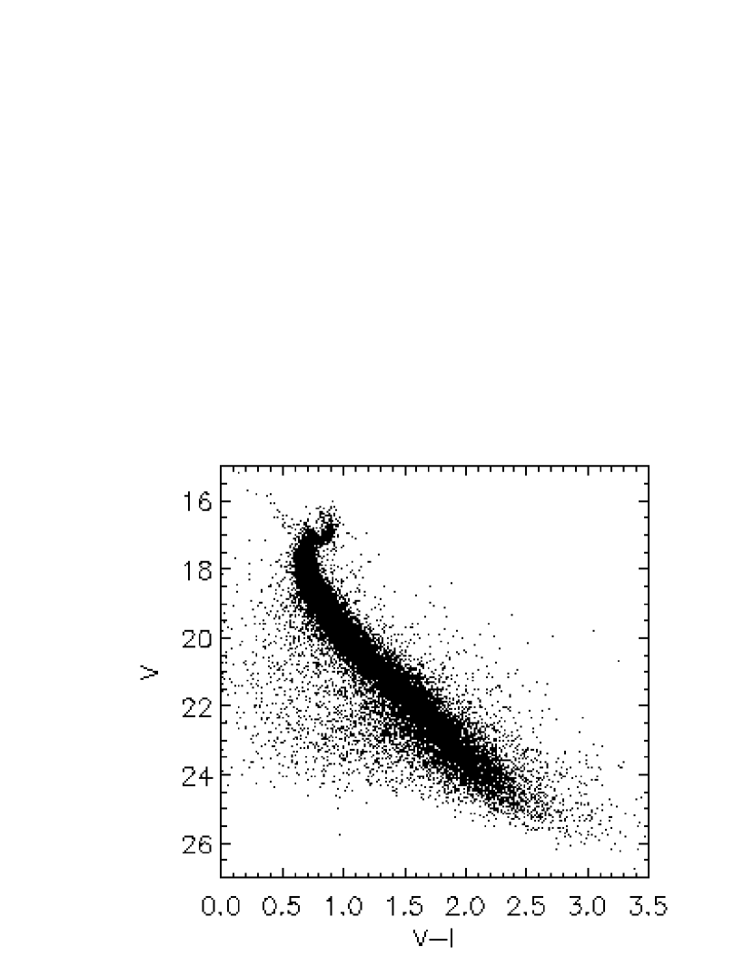
Figure 1: The combined 47 Tuc color-magnitude diagram for all four WFPC2 CCDs for the sample of 46422 stars that remain unsaturated in the primary exposures.

The absolute photometry used here incorporates all standard corrections for CTE with WFPC2 (Whitmore, Heyer, & Casertano, 1999) and filter color terms from Holtzman et al. (1995). Zero points were determined by matching the magnitudes of identifiable portions of the cluster main sequence to those measured for 47 Tuc by other investigators. $V$ has been set by forcing $V$ = 17.14 for a first moment centroid over $0.78<(V-I)<0.83$. This value was selected as a representative average of Hesser et al. (1987) ($V$ = 17.12), unpublished results from RLG (17.14), Kaluzny et al. (1998b) (17.20), and Alcaino, & Liller (1987) (17.22). For $I$, an adjustment to $V-I$ = 0.69 is forced over 17.48 $<$ $V$ $<$ 17.73, based on values for the position of bluest extent of the main sequence from Alcaino, & Liller (1987) ($V-I$ = 0.68) and Kaluzny et al. (1998b) (0.71). Systematic errors of 0.05 magnitudes for the zero point uncertainty of the absolute photometry scales should be carried. The color-magnitude diagram from all four CCDs combined is shown in Fig. 1.

To generate time series for each star, the oversampled representation was subtracted from each individual image by evaluating it at the appropriate dither position and convolving with a compensation kernel, calculated for each frame to represent focus variations due to thermal changes in the telescope. Difference-photometry time series were developed for each star by fitting a PSF (evaluated from isolated stars in each direct image) at the known star position in the difference images. The resulting counts in the time series were then normalised by the total expected in direct images based on star-by-star magnitudes. These time series were cleaned by removal of residual, small linear correlations with changes in the ensemble-average relative intensity and with terms up to cubic in the combination of $x$ and $y$ dither locations.

The difference-image photometry approach (e.g., see Alard (1999), and Alcock et al. (1999)), as extended here to under-sampled data, provides near-optimal results even for stars that are strongly blended with neighbors. As shown in Gilliland et al. (2000), time series precisions range from 0.003 near cluster turnoff at $V\>\sim$ 17, to 0.01 at $V\>\sim$ 19.5, 0.03 at $V\>\sim$ 21, and 0.1 at $V\>\sim$ 23, extending the earlier results beyond the limit for which giant planets might be detected. The difference-image photometry solutions are intimately linked with the process that develops the over-sampled combined images. In particular, the underlying assumption is that the intensity registered for any pixel can be represented as a function of a constant source and changes only as a result of $x$, $y$ offsets and focus changes image-to-image. Thus for the vast majority of non-variable stars precisions near the fundamental limit imposed by Poisson statistics of the source, background and readout noise are maintained.

For large-amplitude variables, excess noise can arise since the solution may not properly decouple intensity changes in a given pixel that arise from $x$, $y$ offsets of under-sampled PSFs rather than intrinsic variations. This makes the time series of some variables noisier than for non-variable stars at similar magnitudes. We have investigated the characteristics of this excess “model” noise in some detail. For all the variable stars we detect, we calculate the magnitude of the model noise by subtracting in quadrature the mean rms for non-variables of the same $V$-magnitude from the rms scatter of the variable star measured from bins of 0.05 in phase. (By measuring in such small phase bins we eliminate most of the intrinsic variability.) In Fig. 2 we plot this excess noise as a function of amplitude for the variables stars we detected on the PC1 CCD with $17<V<19$. It is clear that the model noise of the detected variables scales with amplitude of variability. The upper limit in the non-variable population is 5 mmag. (The few stars that lie above this boundary are affected by cosmetics such as diffraction spikes from nearby saturated stars and show photometric variations at the HST orbital frequency.) Such plots for other CCDs and magnitude ranges show similar behaviour, although the derived upper limit is obviously higher for fainter magnitudes.

To illustrate the relative unimportance of this excess model noise for variable star detection, we consider the following scenarios. At amplitude 0.1 mag, the model noise is $\sim$ 0.015 mag. Given our time coverage with about 600 points in each of the $V$ and $I$ bandpasses, we ask what is the signal-to-noise of a coherent signal with amplitude 0.1 mag and noise 0.015 mag. From Scargle (1982), the signal-to-noise of the peak periodogram power is $N(A/2\sigma)^{2}$, where $N$ is the number of observations, $A$ is the signal amplitude and $\sigma$ is the noise. If the model noise dominates the intrinsic rms noise, the S/N in each bandpass is greater than 6000. If we consider the regime where $A=0.02$ mag with model noise 0.004 mag, a bright star will have a similar level of intrinsic noise so that the total noise (adding in quadrature) is $\sim$ 0.006 mag. The S/N is then $\sim$ 1000 per bandpass. If the amplitude is only 0.002 mag, even retaining the same noise level still gives a S/N of $\sim$ 17 per bandpass. For fainter stars, the intrinsic noise is always dominant at low signal levels. In summary, for small intrinsic amplitudes, excess model noise is negligible in comparison to the intrinsic noise; by the point at which large amplitudes may lead to significant excess noise, the variation is sufficiently large to be quite obvious.

In many cases the initial variability search returned multiple variables with similar periods in close spatial proximity. Where stars are close enough that their point spread functions overlap to a significant degree (which is common in such a crowded field) the extracted time series for each will reflect the variability. In order to determine which of several blended stars is the true variable, we used the measured time variation to choose difference images near both the maximum and minimum for each variable. We then subtracted the average of the near-minimum images from the average of the near-maximum images. This phased, difference-image sum was then compared to a sum of the direct images for the same exposures. The true variable appeared in the difference-based sum as an isolated PSF; comparison with the direct image then provided a secure identification of the intrinsic variable. Instances were found in this way of apparently-bright, low-amplitude variables having arisen from blending with nearby fainter variables with intrinsically large amplitudes. Also, cases were turned up in which an apparent faint variable resulted from contamination via the wings of a moderately-distant, saturated, intrinsically-variable star.

As noted at the beginning of this section, our observations were all taken at a single pointing, with the center of the globular cluster on the PC1 CCD. Out to a radial distance of $\sim$ 10 arcseconds, our area coverage is complete. Beyond this, the non-uniform shape of the array of WFPC2 CCD’s meant that our spatial sampling was lower. In several parts of the remainder of this paper, we calculate binary-frequency statistics from our observations. Since we expect binary stars to have a different degree of central concentration than single stars (this is born out in § 7), we need to be aware of bias which may be introduced by the non-uniform radial sampling of our survey. To this end we have calculated the radial area completeness function (Fig 3) which we use later to correct our statistics. For consistency with Howell, Guhathakurta, & Gilliland (2000), we take cluster center to be at J2000 coordinates (00:24:05.87, -72:04:51.2) from Guhathakurta et al. (1992). Such a correction implicitly assumes azimuthal symmetry for the cluster. Normally our correction will be to a circular region within 90 arcseconds of the cluster center.

3 Variable Stars

The time-series data were searched for variability by several different methods. For near-sinusoidal signals, the Lomb-Scargle (LS) periodogram is the most useful search technique. For some other types of variability, such as the lightcurves of detached eclipsing binaries, the LS periodogram is rather insensitive. In order not to miss any non-sinusoidal variability we searched for lightcurves where the mean of the lowest five consecutive points deviated from the lightcurve mean by a factor of 2 or more times that of the highest five points (this test is sensitive to eclipsing binaries) and vice versa (sensitive to microlensing or flaring phenomena). In practice, all the variable stars found by this method were also found with the LS method. All of the variables found in the primary search (of a smaller subset of 34091 stars) for planet transits using matched-filter-convolution approaches that are optimally sensitive to detecting repeated eclipses (Gilliland et al. (2000), Brown et al. (2001), in preparation) were recovered with these independent searches.

The 160-$s$ time-series exposures were obtained at 240-$s$ intervals, providing a formal Nyquist sampling frequency of 180 $d^{-1}$. The LS periodogram was thus calculated over the period range $0.005-10.0$ $d$, frequencies $0.1-200$ $d^{-1}$.

In order to investigate the appropriate cutoff point for LS false alarm probabilities in our time series, we have calculated 10 000 Gaussian-noise time series at the same sampling as our data. These were passed through the same LS analysis and the highest periodogram peak and its false alarm probability evaluated for each. The lowest false alarm probability recorded in each of the $I$- and $V$- band simulation sets was $1.26\times 10^{-4}$. Guided by this we set the false alarm probability threshold at $10^{-4}$ for the analysis of our data. The lightcurves for all stars in our sample having a LS false alarm probability less than this were examined in more detail. We excluded from this procedure periods within $1\%$ of a multiple of $1$ or $2$ times the HST orbital period (96.66 minutes). In order to pass our test for variability, we required that a peak greater than the false-alarm probability threshold be present in either the $I$- or $V$-band power spectra and that a peak at the same frequency be recognisable by visual inspection of the power spectrum of the other band.

In order to test our ability to find regular variability, we have performed tests with simulated data. Sinusoidal signals of random frequency and phase were injected into the lightcurve data for random stars (excluding the small fraction of stars which had been found to be variable) from the PC1 and WF2 CCDs. Because we sample randomly from the population of non-variable stars, the actual distribution of noise is automatically taken into account. The chosen periods were drawn with equal probability in $\log P$ over the range $0.005<P<12$ days. The same amplitude was used for $V$ and $I$, with discrete values $\frac{\delta(intensity)}{intensity}=(0.002,0.005,0.010,0.020,0.100)$ and with $100,000$ simulations for each amplitude. The resulting simulated lightcurves were passed through the same search procedure as the real data. From this we have characterized our variability recovery rate as a function of signal-period, signal-amplitude and mean $V$-magnitude (Fig. 4). The recovery rate is relatively independent of period except at the long period end where there is a drop-off in sensitivity.

In Fig.5 we plot the fraction of the recovered variables for which the period was determined correctly to within 10% of the input period. There is a rapid decrease at the long-period end, especially for low-amplitude signals. For example, this implies that at magnitude $V=20.5$ only half of the variables we have detected with half-amplitudes $\sim 5$ mmag will have periods accurate to within $10\%$. This is not as problematical as it may seem since (see Fig. 4) our recovery rate is already low in this regime.

A total of 114 variable stars were detected out of the 46422 non-saturated stars found on the four CCDs. Nearly all the variable stars detected are believed to be binaries. At periods from 0.2 days extending up to 1.1 days we find a number of contact binaries with obvious W UMa lightcurves. Interspersed in period with these, and with periods extending up to the $\sim$ 10 day limit to our sensitivity, are many regular variables with near-sinusoidal to decidedly non-sinusoidal lightcurves. We interpret these stars as being BY Draconis variables - rotating, chromospherically-active main-sequence stars. Since the timescale for spin-down of a young main-sequence star is vastly shorter than the age of 47 Tucanae, these stars must also be in (presumably tidally affected) binary systems. In addition (but not distinct from the previous category) we find a number of eclipsing systems. Finally, there are a few stars which do not fit into these categories.

In this paper we adopt a convention where we number variable stars separately for each of the four WFPC2 CCDs. Since the PC1 field overlaps with our previous observations (Edmonds et al., 1996; Gilliland et al., 1998), we keep the same numbering for the variable stars found in those studies. Thus (PC1-V01,…,PC1-V16) in this paper are the same stars as (V1,…,V16) in Edmonds et al. (1996) and Gilliland et al. (1998). For the other CCDs we begin numbering from unity (e.g. the variables found in the WF2 field are named WF2-V01, WF2-V02,…).

4 Detached Eclipsing Binaries

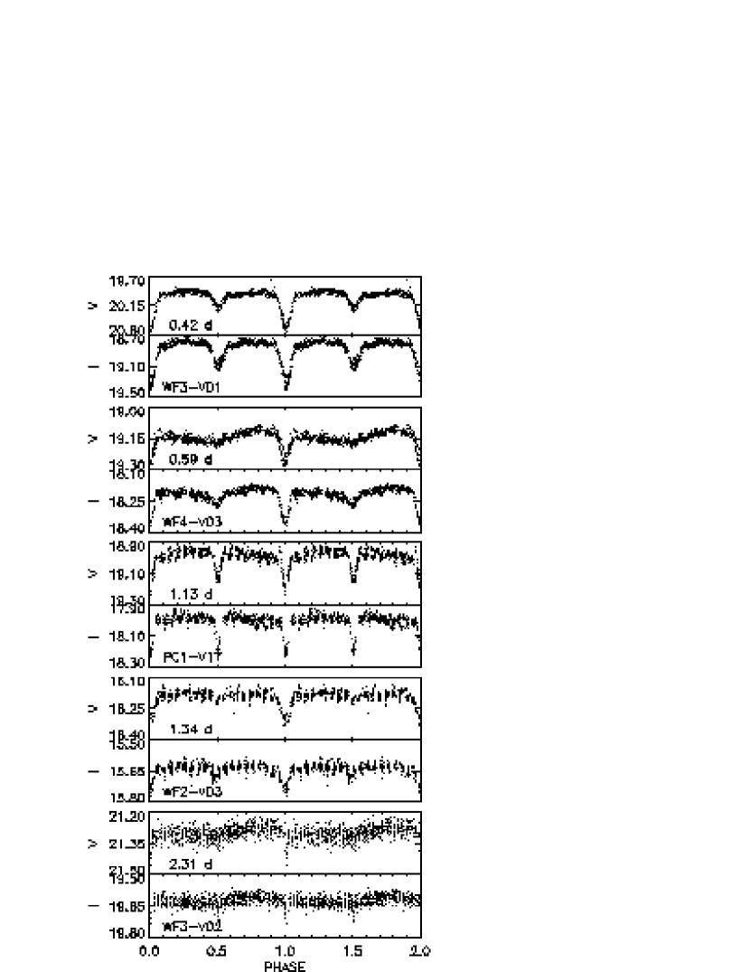
Figure 6: Lightcurves of eclipsing binaries with periods shorter than 4 days. Upper panel of pairs provides F555W results with F814W in the lower panel. Periods in days and reference names corresponding to Table 1 entries are displayed for each case.

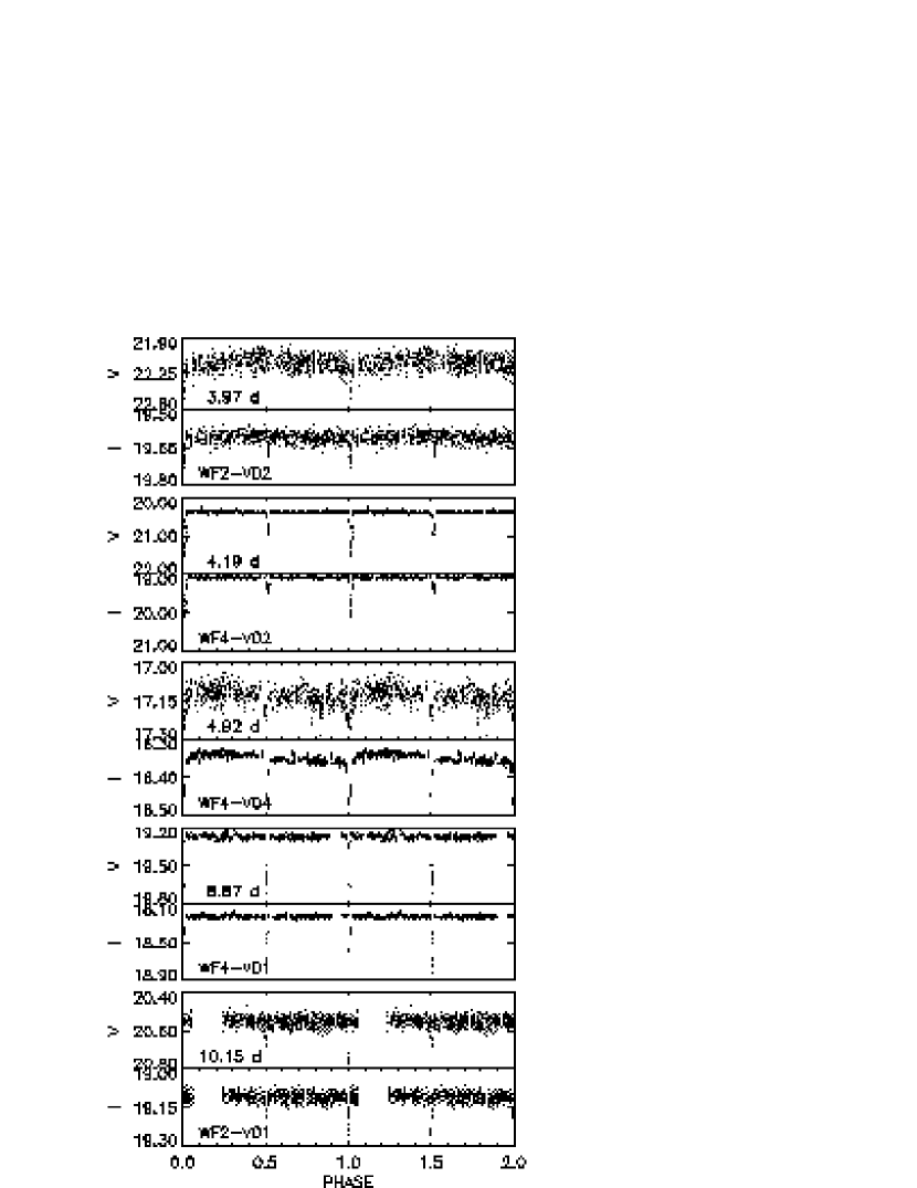
Figure 7: Lightcurves of eclipsing binaries with periods $\gtrsim$ 4 days.

Ten of the stars in our sample (Figs 6,7, Table 1), by visual examination, are obvious detached eclipsing binaries with characteristic primary and secondary dips in their lightcurves. An additional eclipsing binary was found which showed only one eclipse during our observation period and this is grouped with the miscellaneous variables in §8. The periods of eclipsing binaries we observe today may not be their primordial periods. Over time, tidal effects tend to circularize and then bring together initially-detached binaries. The upper cutoff period for tidal circularization increases with age and is likely to be in the range 13–18 days for a population with age of 47 Tucanae (Mathieu, 1994). With subsequent angular momentum loss, many binaries with periods less than some cutoff period will have evolved to significantly shorter periods during the lifetime of the cluster. We have used the model of Vilhu (1982) (see also Bradstreet & Guinan (1994)), through which the decrease of spin angular momentum by magnetic braking is coupled to an increase of orbital angular momentum (and hence a shorter period) to calculate this cutoff period. Applied to a 0.9 $M_{\odot}$ star, we calculate that 4 days is the cutoff period for binaries in 47 Tuc with mass ratio $q\sim 0.3$. Those with smaller q would have evolved to contact in less than 11 Gy. (Note that this model does not apply to very low values of $q$, such as for planets, where there is no significant tidal affect on the more massive component.) For binaries where $q\sim 0.9$, none would have evolved to contact over the cluster lifetime, assuming they had primordial periods greater than 2.5 days.

We thus consider here the five eclipsing binaries with periods $\gtrsim$ 4 days as being an “unevolved sample” and ask what their numbers imply about the fraction of primordial binary stars in the core of 47 Tuc.

We assume that we have detected all the binary stars in our sample which show two eclipses during the time span of the observations. This places an upper limit of $\sim$ 16.6 days to the periods we could have detected, assuming that both primary and secondary eclipses are visible. Using Kepler’s third law and geometry, the probability of detecting eclipses in a given binary with magnitude $V$ and period $P$ in days is

$$D(V,P)=\frac{\zeta R_{1}+R_{2}}{4.21(M_{1}+M_{2})^{1/3}P^{2/3}}\times\max(0,\min(1,\frac{2\tau_{obs}}{P}-1))$$ (1)

where $M_{1},M_{2}$ and $R_{1},R_{2}$ are the mass and radius in solar units of each component (inferred from $V$), $1-\zeta$ is the minimum fraction of the eclipsed star’s radius we require to be obscured for a detectable eclipse and $\tau_{obs}$ is the observation period, 8.29 days. For any assumed mass ratio, the masses and radii of the components can be drawn from a suitable isochrone after allowing for partition of the observed luminosity between each star in the appropriate ratio.

For a flat primordial frequency distribution of binaries, $\frac{df}{d\log P}=\beta_{0}$, where $f$ is the cumulative fraction of binaries with periods less than $P$,

$$f_{0}=\beta_{0}(\log P_{max}-\log P_{min}),$$ (2)

where $f_{0}$ is the fraction of primordial “hard” binaries (those where the orbital velocity is greater than the velocity dispersion of the cluster). “Soft” binaries are expected to be quickly disrupted through interactions with other stars (Hills, 1984). The central velocity dispersion of 47 Tuc is 11.6 km s^-1 (Meylan & Mayor, 1986), implying a maximum orbital period for “hard” binaries of $\sim$ 50 years. (This limit will be smaller if a sufficient binary population exists to allow the larger cross sections of binary-binary interactions to be important in disrupting systems.) $P_{min}$ = 2.5 d is the minimum observed period in zero-age binary star populations (Mathieu, Walter, & Myers, 1989). Thus, for an observational sample with $N_{V}dV$ stars in each $V$-magnitude interval $dV$, the number of eclipsing binaries we expect to detect over a period range $P_{1}$ to $P_{2}$ and magnitude range $V_{1}$ to $V_{2}$ is

$$N_{P_{1},P_{2}}^{eclipsing}=\int_{V_{1}}^{V_{2}}\int_{\log P_{1}}^{\log P_{2}}N_{V}D(V,P)\beta_{0}d\log PdV,$$ (3)

which is a linear function of $f_{0}$.

Figure 8 shows this relation for 47 Tuc, where we have used the 11 Gy VandenBerg (2000) isochrone for the masses and radii, have assumed equal masses, and that $\zeta=0.9$. We have detected five eclipsing binaries with periods between 4 and 16 days, which implies that the primordial hard binary fraction of the cluster core is 13 $\pm$ 6 %. For this calculation and in the remainder of this paper we define the binary fraction as being the number of binary stars relative to the number of main sequence stars searched. The error we quote here is due entirely to the $\sqrt{n}$ Poisson uncertainty in the number of detections, which far outweighs internal errors in any of the measurements or parameters. For instance, using $\zeta=0.8$ increases the derived binary fraction by less than 1% and using a mass ratio $q=0.5$ increases the derived binary fraction by $\sim$2%.

We can also examine the sensitivity of our model to assumptions about the binary period cutoff and the shape of the frequency distribution. If the efficiency of disruption of binaries is much greater than expected and the upper limit to binary periods is 5 years rather than 50 years, then the binary fraction we derive is 10 $\pm$ 4 %. If the frequency distribution of binaries is not flat, but rather follows the exponential function of Duquennoy & Mayor (1991) (found from nearby G dwarfs), $f=\beta_{0}e^{-0.095(\log P-4.8)^{2}}$, the derived binary fraction becomes 17 $\pm$ 8 %.

As noted in § 2, our observations are subject to bias because of radial incompleteness in the area coverage. For the eclipsing binaries considered here, the correction factor is negligible, changing the estimated binary fraction by ¡ 0.2 %.

We can ask whether the periods of the stars we have detected are consistent with flat or exponential distributions. In practice, $D(V,P)$ is almost independent of V, thus simplifying a search for period dependence. Unfortunately two of the five eclipsing binaries being considered each show only two eclipses during the time of observation so there is a slight ambiguity as to whether these are primary and secondary eclipses (in which case the periods are 8.87 and 10.15 d) or primary eclipses only (in which case the periods are half these values). In fact, detailed inspection of the lightcurves argues for the former. For WF4-V01, the depths of the two observed $V$–band eclipses differ. For WF2-V01, the depths of the two observed eclipses are very similar but there is no apparent eclipse at the phase midway between them. If there was an unobserved secondary eclipse at this phase then this would place such a small upper limit on the radius of the secondary that the primary eclipse would have a flat bottom, which is not the case. In Fig. 9 we show the cumulative period distribution compared with the models for flat and exponential distributions. The cumulative distribution is driven mainly by the geometric factor for probability of eclipses given random orientations, so in practice does not provide a good discriminant between models. The Kolmogorov-Smirnov statistic (Press et al., 1992) for the maximum difference between the distributions of the flat model and observed periods is 0.33 with a formal probability of 54% that the observations are drawn from the model population.

5 W Ursa Majoris Binaries

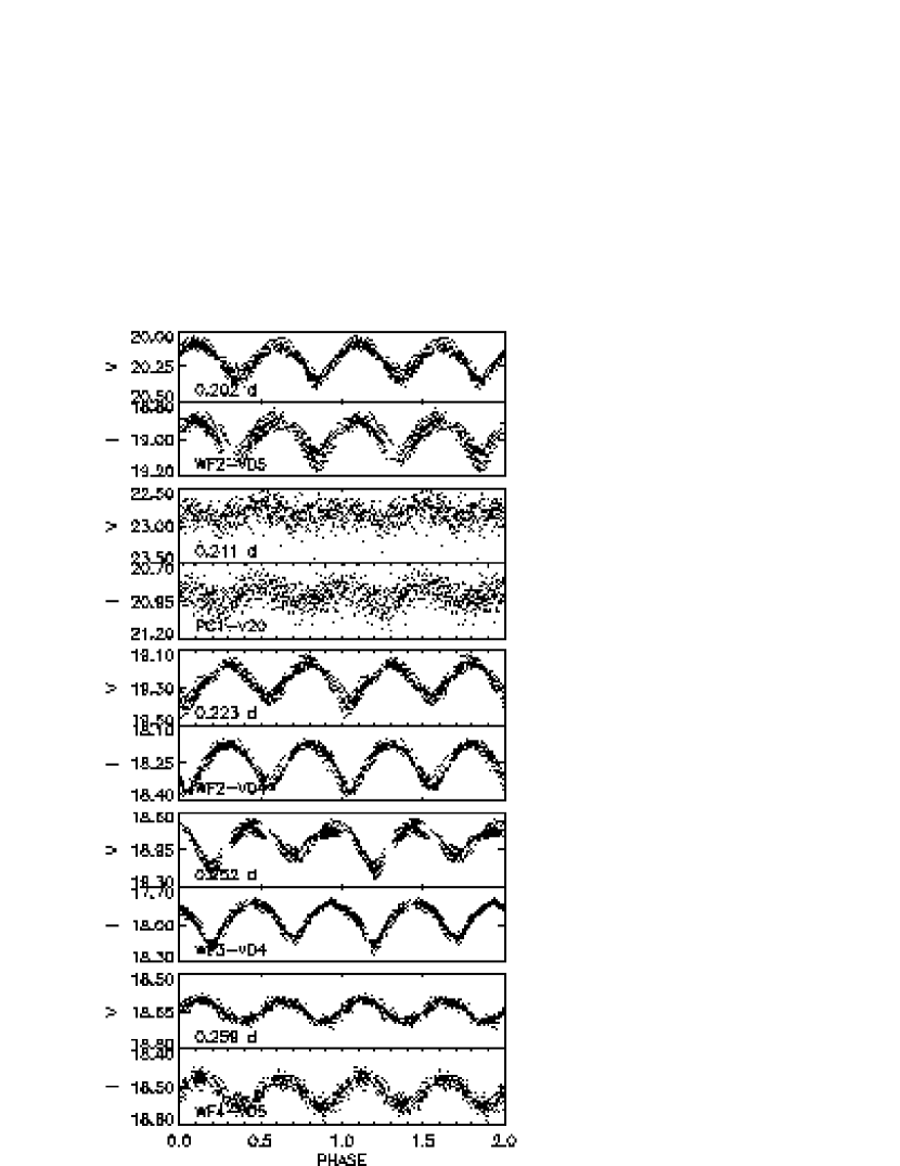
Figure 10: Lightcurves of W UMa and near-contact binaries.

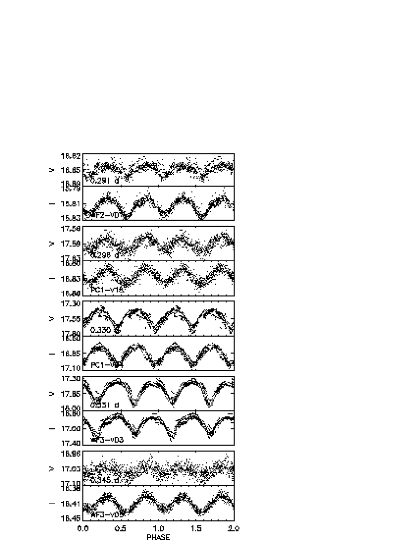
Figure 11: Lightcurves of W UMa and near-contact binaries.

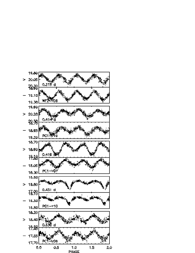
Figure 12: Lightcurves of W UMa and near-contact binaries.

Fifteen of the stars in our sample have, by visual examination, characteristic W UMa lightcurves (Figs. 10, 11, 12, Table 2). These were initially assumed to be contact binary systems. The generally accepted theory for the formation of such systems is that detached binaries lose orbital angular momentum by a magnetic braking mechanism when their spin and orbital angular momentum become tidally coupled (Vilhu, 1982; Eggen & Iben, 1989). The rate of approach increases as the separation decreases because the strength of the magnetic stellar wind increases with higher rotational velocities (Skumanich, 1972). For nearly equal mass stars, a rapid initial mass transfer will occur after first contact is established (Flannery, 1976; Robertson & Eggleton, 1977; Iben & Livio, 1993) because, for a main sequence star with a convective envelope, the Roche-lobe radius shrinks faster in response to mass loss than does the stellar radius. Subsequent mass-transfer oscillations (for part of which time the system may be in a semi-detached state) result in a system with mass ratio varying over the range $0.61<q<0.79$. An important consequence is that the total luminosity of a nearly-equal-mass pre-contact binary will increase as the system adjusts to a different mass ratio (Vilhu, 1982). For instance, a binary with initial component masses of 0.75 $M_{\odot}$ will be brighter by 0.34 mag after it evolves to a mass ratio $q=0.8$. The brighter component will also be bluer leading to a tendency for bright W UMa systems to be blue stragglers.

As shown by Rucinski (1994, 1995), contact binaries are observed to obey a period-luminosity-color-metallicity relation,

$$M_{V}=-4.43\log P+3.63(V-I)_{0}-0.31-0.12[Fe/H],$$ (4)

with P in days and $M_{V}$ magnitude at maximum. In Fig. 13 we show the apparent distance modulus of the W UMa stars as a function of their periods, where we have used Eqn. 4 and followed Kaluzny et al. (1998a) in assuming $[Fe/H]=-0.76$ and $E(V-I)=0.05$ (Harris, 1996). For reference, the apparent distance modulus of 47 Tuc listed in Harris (1996) is $(m-M)_{V}=13.37$ while Zoccali et al. (2001) found $(m-M)_{V}=13.27$. In the diagram, we have grouped the stars into those that are consistent with the Rucinski calibration (Group 1) and those that are not (Group 2), plotted as different symbols. The criterion we used for Group 1 membership was that a star had an apparent distance modulus within 0.3 magnitudes of 13.1 in Fig. 13. We retain these groupings and plot the color-magnitude diagram (Fig 14) and period-luminosity diagram (Fig 15) for the same stars. In Fig. 15 we also show fiducial lines representing equal-mass Roche-lobe filling and primary and secondary Roche-lobe filling for a binary with mass ratio $q=0.61$. These lines were calculated using the condition that the radius of each component star is equal to the volume-averaged radius of its Roche lobe (Paczynski, 1971; Eggleton, 1983),

$$R_{L}=\frac{0.49q^{2/3}a}{0.6q^{2/3}+\ln(1+q^{1/3})},$$ (5)

where $q$ is the mass ratio and $a$ is the separation. The orbital period follows from Kepler’s third law, taking the main-sequence masses and radii from the Z=0.004 Padova isochrone (Bertelli et al., 1994). (We use here the Padova isochrone because it extends further down the main sequence than the Vandenberg isochrone used in §4.) The 11 Gy isochrone was used for the secondary component but for the primary-star we used the 1 Gy isochrone. This is appropriate because, assuming the binaries have not been in contact for a time comparable to the cluster age, mass transferred to the primary will not have caused it to evolve off the main sequence (i.e. it will appear in a retarded evolutionary state relative to single stars in the cluster with the same mass).

The Group 1 stars all lie on or very close to the binary main sequence in Fig 14 or are blue stragglers. In Fig. 15 these stars are found on or very close to the equal-mass main-sequence critical contact line or (for the brightest few stars) are consistent with being secondary-Roche-lobe filled binaries with mass ratios $\sim 0.8$. These stars are normal contact binaries.

The stars in Group 2 do not obey the Rucinski calibration and require other explanations. The star that deviates the most from the calibrated absolute magnitude (WF4-V05) lies on the equal-mass critical contact line in Fig. 15 but is found far to the blue of the main sequence in Fig 14. The lightcurve (Fig. 10) appears to have unequal eclipse maxima indicating a semi-detached system. The very blue colors may indicate mass transfer from the secondary causing a hot spot on the surface of the primary or a surrounding accretion disk. The star may be a cataclysmic variable.

The star in Fig. 13 with the next-highest positive deviation (WF2-V06) also has rather blue colors but this time is found on the long period side of the Roche-lobe-filling lines in Fig. 15. This star may be a semi-detached low-mass ratio binary undergoing mass transfer.

The star which falls below the Rucinski calibration in Fig. 13 (WF2-V07) is a subgiant. In Fig. 15, it lies close to the line of primary Roche-lobe filling for $q=0.61$, so should be a contact binary if $q\gtrsim 0.6$. Since it deviates strongly from the Rucinski calibration, it may have a low mass companion and be a semi-detached system.

The four remaining Group 2 stars have longer periods than the secondary-Roche-lobe-filling condition for $q=0.61$ (Fig. 15) and lie below or just on the equal-mass binary main sequence (Fig. 14). These are most probably semi-detached systems.

We can use our Group 1 stars to re-derive a distance modulus to 47 Tuc based on the Rucinski calibration. The mean distance modulus of our 8 Group 1 stars is $(m-M)_{V}=13.10\pm 0.15\pm 0.23$ where the quoted uncertainties are random followed by systematic. (We have assumed systematic uncertainties of 0.05 mag in $V$ and in $V-I$. A reduction in these with more definitive absolute photometry, particularly for $V-I$, could significantly lower the systematic error on the distance modulus.) This can be compared with the recent Zoccali et al. (2001) value $(m-M)_{V}=13.27\pm 0.14$ based on the position of the white dwarf cooling sequence. We note that Zoccali et al. (2001) used $E(B-V)=0.055$ which, with $A_{V}=3.2E(B-V)$ and $A_{I}/A_{V}=0.6$ (Schlegel et al., 1998), corresponds to $E(V-I)=0.072$. If we use this value, rather than $E(V-I)=0.05$ (Harris, 1996), then we derive $(m-M)_{V}=13.17\pm 0.15$, in agreement with Zoccali et al. (2001). The W UMa-derived distance modulus favors a distance at least as low as the white dwarf-determined value.

The timescale for initially-detached binaries to evolve to contact is rather poorly known. The model of Bradstreet & Guinan (1994) predicts that binaries with primordial component masses $\sim$ 0.7–0.9 $M_{\odot}$ and mass ratios greater than $\sim$ 0.7 will have evolved to contact in a cluster-age time if their initial orbital periods were $\sim$ 2–4 days. (Values of $q$ near unity and lower masses give the longest initial orbital periods.) Binaries with periods longer than this will not have undergone a significant change in their orbital period due to magnetic braking over the cluster lifetime. We assume the lowest primordial orbital period is 2.5 days and the highest that could have evolved in the age of 47 Tuc to contact is 4 days.

After contact is established, estimates of the timescale for a binary to merge and become a single star are $\sim 10^{9\pm 1}$ years (Vilhu, 1982; Rahunen, 1981). Out of the 46422 stars we have observed, we have estimated that 15 are the contact or near-contact products of angular-momentum-loss evolution. The observed W UMa frequency of our sample is therefore 0.032 %. Because of non-uniform area coverage, our survey is skewed towards preferential detection of variables within 10 arcseconds of the cluster center (see § 2). We can correct for this bias by weighting each star by the inverse of the radial area completeness function (Fig 3), which we use out to a radial distance of 90 arcseconds. Applying this correction, we have 22.6 W UMa stars detected out of a total of 67004.6 stars. Thus the true observed W UMa frequency within 90 arcseconds of the cluster center is 0.033 %, one per 3010 stars. This is an order of magnitude lower than the rate of one W UMa per 250-300 main-sequence stars in the disk of the Galaxy (Rucinski, 1997). It is also about 1.5 times higher than (but probably in statistical agreement with) the observed main-sequence W UMa frequency in the previous HST survey of the core of 47 Tuc by Edmonds et al. (1996). Our observed frequency is three times higher than the frequency observed by Kaluzny et al. (1998a) over a large area surrounding but outside of the core. This result is not unexpected since there is an appreciable mass segregation in 47 Tucanae (see §7).

Doubling the observed number of W UMa’s to allow for unfavorable orientations for eclipses and adopting $10^{9}$ years for the contact-binary lifetime requires that 1 new contact binary be formed every $2.2{\times}10^{7}$ years from our sample. Over the 11 Gy lifetime of the cluster, $\sim$ 490 such contact systems would have formed. If all the binary systems with primordial periods between 2.5 and 4 days have evolved to contact or near-contact then our numbers imply a primordial binary frequency of 0.73% for those with initial orbital periods between 2.5 and 4 days. If we make the further assumption (as in §4) of a flat distribution of primordial binaries with $\log P$, this implies a total primordial binary fraction of 14 $\pm$ 4 % (where the quoted error is the lower limit from Poisson statistics). This result is in remarkable (but likely fortuitous) agreement with the value derived from longer period eclipsing binaries in §4. We stress that the binary frequency derived here is inversely proportional to the adopted contact binary lifetime. If the lifetime is $10^{10}$ years rather than $10^{9}$ years then the derived binary frequency becomes 1.4 $\pm$ 0.4 %.

In order to compare our value with that for field stars in the solar neighbourhood, we adopt both a field-star binary frequency (65 %) and the ’exponential’ period distribution from Duquennoy & Mayor (1991). Considering only periods between 2.5 days and 50 years, this binary frequency among solar-like stars is 26 %. Thus, given the assumptions that entered our calculations, the binary frequency in the core of 47 Tuc (within 90 arcseconds of the center) is about half the frequency among field solar-type stars.

6 Other short-period variables

In addition to those binaries discussed above, we have found a further 15 photometric variables with doubled periods (i.e. twice the observed periods) of between 0.1 and 1.5 days. Classification of these stars as contact or semi-detached binaries or BY Dra stars is not possible on the basis of lightcurve morphology (in the majority of cases) because the amplitude of variability is too low. Some of them (particularly with periods less than 0.6 d) may be either contact or semi-detached binary systems where the orbital inclination is low relative to the plane of the sky. In these stars the orbital period will be twice the period we detect.

Others have clearly non-sinusoidal lightcurves. These stars are unlikely to be pulsators since they are not found in any particular variable-star region of the color-magnitude diagram. From Hesser et al. (1987), we estimate that at most 2 stars in our sample could be SMC horizontal-branch stars (most of which would be non-variable) and these would appear to the blue of the 47 Tuc main sequence at $V=19.4$. Our provisional interpretation is that they are most likely BY Draconis variables. These are defined as low amplitude variables with periods of a few days where the source of variability is rotational modulation by starspots (Bopp & Evans, 1973). In these cases the rotation period is the same as the photometric period. Amplitudes of photometric variability are typically a few hundredths to a few tenths of a magnitude in $V$ (Cutispoto, 1993) although there is probably a strong selection effect against discovery of lower amplitude variables. Spectral observations of nearby BY Dra stars imply that many but not all of them are binaries (Bopp & Fekel, 1977) but that rapid rotation is the condition necessary for the BY Dra phenomenon (Vogt, Penrod, & Soderblom, 1983). Since the spin-down time for primordial rotating single stars is small compared to the age of 47 Tuc (Skumanich, 1972; Soderblom, 1983; Siess & Livio, 1997), the stars in our sample are also likely to be tidally coupled binaries.

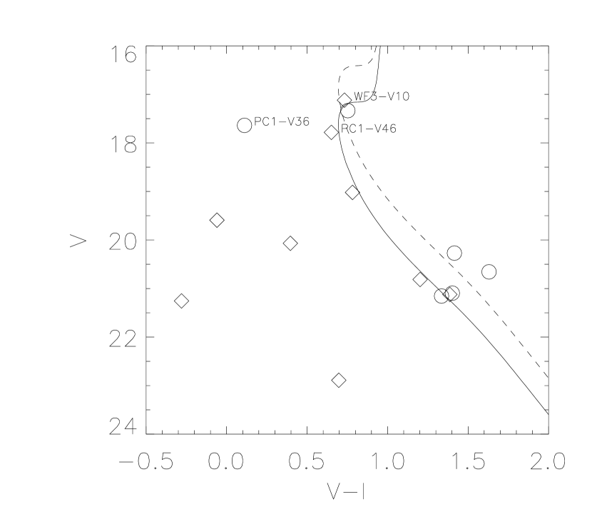
Figure 17: Color-magnitude diagram of the short-period non-eclipsing variables. The solid line is the fiducial ridge line for 47 Tuc. The dashed line is this line shifted upwards by 0.75 mag, i.e. the equal-mass binary sequence. Symbols are as in Fig. 16.

As mentioned earlier, classification of most of these low-amplitude variables from their lightcurve morphology is not possible. To ask which of them are consistent with being contact binaries, we again turn to the absolute magnitude calibration of Rucinski (1995) (Fig. 16) and the period–luminosity (Fig. 18) and color–magnitude (Fig. 17) diagrams.

In Fig. 16 we indicate the box where the contact W Uma binaries were found in §5 and divide the stars into two groups based on their (double) periods. There is an apparent period gap between 0.4 and 0.8 days and we hypothesize that the double period is incorrect for the longer period group. From Fig. 18, even the single periods of these stars are generally too long for secondary Roche lobe filling and their absolute magnitudes are inconsistent with the Rucinski calibration for contact binaries. In Fig. 17, this group, with one exception, lie on or near the single or binary main sequences. These are most likely BY Draconis stars. We note overlap between these stars and the longer period variables considered in §7.

The properties of the one member of this group with very blue colors (PC1-V36) is rather puzzling. In the period-luminosity diagram Fig. 18 it lies in the region where secondary Roche lobe filling should have occured if the period we observe (0.4 d) is the rotation period, not half the rotation period. If the Roche lobe has been filled however, we should observe ellipsoidal variability at half the rotation period. On the other hand, if the rotation period is 0.8 d then we would not expect Roche lobe filling and the consequential ellipsoidal variability. However, if the secondary star in this system is of very low mass, then Roche lobe filling may still have occurred, even at a period of 0.8 d. The blue $V-I$ colour is indicative of ongoing mass transfer. We suggest this as a likely scenario for this star, and hence that the true rotation period is 0.8d. If this is the case then the star belongs with the short-period group discussed next and is not a BY Dra star.

The short-period group of stars are found in Fig. 16 in the same region or extending above the W UMa binaries in Fig. 13. Stars PC1-V46 and WF3-V10 are consistent with the Rucinski calibration and have periods and luminosities in Fig. 18 consistent with having filled their primary and secondary Roche lobes for $q\sim 0.8$. These are likely to be contact binaries. (We elect to keep them in a separate group from the W UMa stars since our classification is not on the basis of lightcurve morphology.) The remaining stars have blue colors and have periods consistent with being close to secondary Roche lobe filling. These are probably the non-eclipsing counterparts of the mass-transferring semi-detached binaries found in §5. The observed parameters of these non-eclipsing contact or semi-detached binaries are listed in Table 3.

7 Longer-period variables: the BY Dra stars

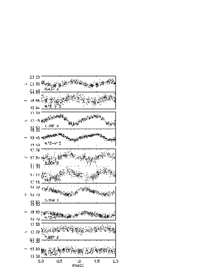
Figure 19: Lightcurves of sample BY Dra stars.

Additional to the stars classified as BY Dra in §6 and extending to periods as long as 10 days, we have found a further 69 variables which we also suspect to be of this type. Sample lightcurves for a representative range of periods are shown in Fig. 19. Several of the variables are of very low amplitude and are only recognized as such through their power spectra.

The color–magnitude diagram for these stars (and also those thought to be BY Dra type in §6) is plotted in Fig. 20. The majority of stars are within the band defined by single and binary main sequences (Table 4). Notable are a group of six red stars in a box slightly below subgiant magnitudes at $V\>\sim\>17.5$ (Table 5, which we discuss further in §7.1), two blue stragglers and three fainter stars with very blue $V-I$ color (Table 6).

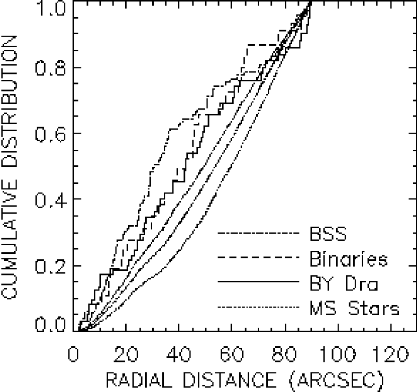
Figure 21: Cumulative distribution with cluster radial distance out to 90 arcseconds of the suspected BY Dra stars compared with binaries (includes contact, semi-detached and eclipsing), blue-straggler stars and main sequence stars from three successive 1.5 magnitude bins below cluster turnoff. The highest MS-star distribution is for the brightest magnitude bin and the lowest is for the faintest bin. The distributions shown have been corrected for radial incompleteness in the area coverage of our survey.

A powerful test of the binary hypothesis for this group of stars is to compare their radial distribution with that of the main-sequence stars in the cluster, the blue straggler stars (BSS) and that of the contact, semi-detached and eclipsing binaries. The cumulative distributions for these samples are shown in Fig. 21 where we have excluded the two blue stragglers, the three very blue variables and the six red stars from the BY Dra sample. (The faint blue variables may be candidates for cataclysmic variables and will be considered in a separate study by Edmonds et al. 2001, in preparation.) These distributions have been corrected for radial area incompleteness using Fig 3. A shoulder in the distributions near a radial distance of 20 arcsec (which was stronger before the radial area coverage correction) is still noticeable. This is due to a higher level of crowding (relative to pixel size) in the WF CCD’s than in the PC at the same radial distance from the center of the cluster. As noted in § 2, our master star list does not contain any stars where more than 90 % of the light within an aperture of radius 5 (PC) or 4 (WF) pixels centered on the source comes from neighbouring stars. Such a bias will preferentially act against fainter stars being included. We have made no attempt to correct for this effect here.

To emphasize the degree of mass segregation in the cluster, we have split the main-sequence stars into three groups; $17.0\leq V<18.5$, $18.5\leq V<20$, $20\leq V<21.5$. The main-sequence stars show an increasing degree of central concentration with brightness, perfectly illustrating the mass-segregation effect. (We have not included corrections for incompleteness as a function of radius and magnitude, but expect such to be small even for the last main-sequence bin which extends only to $V$ of 21.5; these details will be explored in Guhathakurta et al. 2001, in preparation.) The cumulative distributions for the suspected BY Dra stars and the other binaries are very similar and show a higher degree of central concentration than the most massive main sequence stars. The blue stragglers are the most centrally concentrated of all and are likely to be close binaries or their merged remnants. Since the majority of blue stragglers are found more than 0.75 magnitudes above the main-sequence turnoff, at least one of the component masses in these systems is likely greater than the current main-sequence turn-off mass.

To formalize the differences between the distributions, we have used the Kolmogorov-Smirnov test. Applied to the BY Dra and binary samples, the KS statistic (the maximum difference between distributions) is 0.13 with a 85.5% probability that they are drawn from the same population. The difference between the BY Dra and brightest main-sequence group is slightly greater (KS statistic 0.15) with only a 12.5% probability that they are drawn from the same population. This is convincing evidence that our suspected BY Dra stars are indeed binaries.

From the distributions Fig. 21, we can investigate (in a broad sense) how the binary fraction of the cluster changes as a function of radius. Combining the BY Dra and “Binary” distributions, we have compared the fraction of detections in three radius bins, $0\leq r<1$, $1\leq r<2$ and $2\leq r<3$, where $r$ is the radial distance from the cluster center in units of 24 arcseconds, the core radius (Howell, Guhathakurta, & Gilliland, 2000). Scaled to match an overall binary frequency of 13.5 % within 90 arcseconds (an average from §4, 5), the binary frequency in the three radial bins is 20.3 %, 18.3 % and 7.7 %, indicating a relatively constant fraction within two core radii, decreasing rapidly outside of that.

Since the BY Dra stars are presumably the non-eclipsing counterparts of the detached eclipsing binaries discussed in §4, we expect that their amplitudes of variability should be consistent with those of the eclipsing binaries outside of eclipses (that is, the O’Connell effect). In Fig. 22 we plot the semi-amplitudes of variation for these two groups as a function of period, again excluding the blue stragglers and fainter blue variables. As a separate grouping, we include the six red variables from the box in Fig. 20. There is a tendency for variability amplitude to decrease with increasing period. Overall, the distribution of amplitudes is consistent between the BY Dra stars and the eclipsing binaries. Two of the six red variables have amplitudes much greater than the eclipsing binaries.

The large population of BY Dra variables was unexpected and deserves further comment both as a general class and for what they imply for binary fraction inferences, and also for an interesting sub-grouping of these within the CMD. In order to have enhanced activity we rely on the assumption that the stellar rotation rate is rapid due to synchronous rotation with the binary orbit. The radial concentration of this class of objects (see Fig. 21) supports the assumption that these are binaries. For circular orbits the rotation and binary periods would be equal. If the orbit is eccentric, then the rotation period may be much shorter than the binary period, as driven by the much higher orbital velocity at periastron. The binary S1242 in M67 has $e$ = 0.66 and an orbital period of 31.8 days (VandenBerg, Verbunt, & Mathieu, 1999) based on radial velocities. Gilliland et al. (1991) reported a photometric period of 4.88 days at 0.0025 mag amplitude. VandenBerg, Verbunt, & Mathieu (1999) note that the photometric period corresponds to corotation with the orbit at periastron. With the synchronization timescale scaling as $(a/R_{*})^{6}$ (Keppens, 1997) it is easy to see how such a system can arise.

The timescale for rotational synchronization should be short enough to enforce rapid rotation for all binaries with $P\>\lesssim$ 10 days (or equivalent periastron values), even for systems significantly younger than the age of 47 Tuc, but the theory is complex with uncertainties remaining (Keppens, 1997; Keppens, Solanki, & Charbonnel, 2000). We may reasonably assume that any binaries with periods less than or comparable to our sample length of 8.3 days will have synchronously rotating stars. Vogt, Penrod, & Soderblom (1983) surveyed BY Dra stars and found that whether single or in binaries, rotation was more rapid than for other dwarfs and concluded that 5 $km~{}s^{-1}$ or faster rotation was the underlying cause of BY Dra activity. A rotational velocity of 5 $km~{}s^{-1}$ corresponds to $P_{rot}\>\sim$ 8 days for a 47 Tuc K dwarf with $V\>\sim$ 19.5. The general decline of amplitude with period shown in Fig. 20 is expected, but our recovery rate for BY Dra stars in the cluster depends on the (unknown) underlying distribution of BY Dra star amplitudes.

We may use the BY Dra variables to obtain a lower limit to the binary fraction. We have detected 31 BY Dra stars and 5 eclipsing variables with periods longer than 4 days. If we assume that these represent all the binary stars in our sample in this period range and again make the assumptions of a flat primordial binary distribution with $\log P$ truncated at 2.5 days and 50 years then (after a slight adjustment for area-incompleteness) the total binary fraction is 0.76 %. This is a factor 17 lower than the estimates from the numbers of eclipsing binaries and W UMa stars. In Fig. 22, a significant number of BY Dra stars are detected with millimagnitude amplitudes in $V$ and there may well be large numbers at levels undetectable in our data. From Fig 4, our theoretical detection efficiency drops to close to zero for stars fainter than $V=18.5$ and $V$–amplitudes of 5 mmag. For 1 mmag amplitudes the loss of detectability occurs at $V\sim 17$. Thus, the observed BY Dra frequency is probably low because of incompleteness of the sample, but it is also possible that low-amplitude surface activity is a transient phenomenon in these stars.

The prevalence of BY Dra stars in 47 Tuc emphasizes the importance of including angular momentum loss from stellar winds (e.g.. Keppens, Solanki, & Charbonnel (2000)) in any general consideration of binary evolution once the period has dropped below about 10 days. Single stars (e.g. Sun at 5 Gyr old) are rapidly braked to rotation periods $>$ 20 days at which point activity levels drop. In a binary with forced synchronous rotation, magnetic braking feeds back on the orbit which leads to a decreasing orbital period and hence greater activity in response to increasingly rapid rotation. The large angular momentum reservoir of the binary can force high rotation rates for extended periods. Soderblom (1990) noted that field BY Dra stars are a dynamically young (1 – 2 Gyr) population, hence raising the lifetime issue in using BY Dra stars (or eclipsing binaries) to infer an overall binary fraction. The median period of BY Dra stars surveyed by Soderblom (1990) was 3.0 days, not significantly different from the 47 Tuc sample.

7.1 Red stragglers: a distinct sub-class?

Several stars in Fig. 18 fall well away from the primary stellar sequences (main sequence, binary sequence, subgiants, giants, and blue stragglers). The three stars fainter and bluer than the main sequence may be cataclysmic variables and should not be counted as BY Dra, or related stars. The six stars falling within $17.25\lesssim V\lesssim 17.75$ and well to the red of primary main sequence do not have a ready explanation. We propose to call variables in this region of the color-magnitude diagram red straggler stars.

Inspection of color-magnitude diagrams for fields off the core of 47 Tuc region (Hesser et al., 1987; Zoccali et al., 2001) shows that the background SMC giant branch intersects the 47 Tuc main sequence at $V=20$ and passes through the red straggler region. If the ratio of giants to main sequence stars is similar in the SMC as for 47 Tuc, then from Zoccali et al. (2001) we might expect 1 SMC giant to appear in our red straggler box. However, if the red stragglers were truly background SMC stars then we would expect them to lie in a diagonal sequence in $V,V-I$, not a near-horizontal grouping. A Kolmogorov-Smirnov test of the radial distribution from the cluster center of the five stars plus PC1-V11 (a known cataclysmic variable found in the same location in the CM diagram - see below) compared to the radial distribution of area on the sky covered by the WFPC2 CCDs (SMC stars should be distributed equally in area) gives only a 12% probability that they are drawn from the same distribution.

Noting that (a) these are closest in the CMD to subgiants, and (b) similarly very red variables do not appear at fainter levels to the right of the main sequence suggests that their origin is associated with subgiants or giants. Two stars (S1063 and S1113) in M67 (a rich open cluster, but with order 1% the total population of 47 Tuc) fall in the red straggler region of the CMD (compensating for relative distance modulii they fall within the small $V$, $V-I$ box in Fig 20) and have been explicitly commented on in a number of studies by Belloni, Verbunt, & Mathieu (1998), VandenBerg, Verbunt, & Mathieu (1999), and Mathieu et al. (2000) (where they are referred to as “sub-subgiant” stars). The two M67 stars in the corresponding CMD location are: (a) spectroscopic binaries with periods of 2.82 and 18.4 days, (b) X-ray sources, (c) active stars with both Ca II H & K emission and photometric variability noted. All three referenced studies of these well-observed M67 stars note that no ready explanation for stars in this region of the CMD exist and that their origin and evolutionary status remains unknown. VandenBerg, Verbunt, & Mathieu (1999) do note that in principle a subgiant or giant can become underluminous when it transfers mass to a companion, but also that the high eccentricity of one of the M67 stars (S1063 at $e$ = 0.2 and $P$ = 18.4 days) is hard to reconcile with this since rapid circularization of the orbit is expected during mass transfer. The range of observational data for the corresponding 47 Tuc red stragglers is much less complete as compared to the M67 cases.

The evidence strongly suggests that these variables and the corresponding ones in M67 form a distinct class: not only are they clearly variable, but in a CMD with 40000+ entries, they dominate the membership in the small CMD box that they occupy. From the photometry of the non-saturated stars, 5 out of the 17 stars from Fig. 1 which lie in the red straggler box indicated in Fig 20 are variables. Redward of $V-I=0.94$, 4 out of 5 are variables. We posit that a plausible explanation for these stars is a deflated radius from subgiant or giant origins as the result of mass transfer initiated by Roche-lobe contact by the evolved star, for which the secondary has a lower mass. The subsequent evolution as the orbit contracts will force a smaller stellar radius.

Gilliland (1982) discusses subgiant evolution with mass loss for the long-period cataclysmic variable BV Cen - a star in an analogous state. Indeed, the observed $V$ and $V-I$ for BV Cen (Menzies, O’Donaghue, & Warner, 1986) adjusted for distance and differential reddening also place it within our Fig. 20 red straggler box at a location near that for PC1-V11 (AKO 9). The expected lifetime of stars like BV Cen exceeds 10⁹ years (Gilliland, 1982). We also note that the expanded envelopes of these deflated subgiants/giants will have longer convective turnover timescales (Gilliland, 1985) relative to main sequence stars at the same color or luminosity, and thus smaller Rossby number (rotation period divided by convective turnover timescale). This, coupled with enforced synchronous, rapid (relative to other similar stars) rotation in a short period binary, provides a ready explanation (Gilliland, 1985) for heightened activity such as for WF2-V31 which is an outlier in the amplitude – period diagram of Fig. 22.

It is also interesting to note that the 1.108 day period eclipsing-variable PC1-V11 = AKO 9 (Knigge et al., 2000), which has clear spectroscopic signatures in the UV consistent with a long period CV (i.e., the system contains a white dwarf), falls within this red-straggler domain in a $V$, $V-I$ CMD. The presence of a white dwarf primary and accretion disk leads, however, to a much brighter $U$ magnitude than for the other stars in this $V$, $V-I$ region. BV Cen, as noted above, falls in this domain in $V$, $V-I$ but, like AKO 9 , has a strong UV excess. Perhaps the companions for the other red straggler variables in this domain are main sequence stars, not white dwarfs, which may explain their lack of excess UV emission.

At least two of the six red stragglers detected here have also been detected with Chandra (Edmonds et al., 2001 in preparation), and have X-ray luminosities similar to those of S1063 and S1113 in M67 (Belloni, Verbunt, & Mathieu, 1998) and similar to those of field RS CVns (Dempsey et al., 1997). One other red straggler in 47 Tuc, lying outside our field of view, has been found using archival HST analysis and this star is also likely to be a Chandra source (Edmonds et al. 2001). These observations strengthen our argument that the red stragglers in 47 Tuc and M67 form a distinct class with properties explained by mass transfer, rapid rotation and enhanced activity. We suggest that stars in other clusters falling within this red-straggler domain (e.g. the two stars within this domain in the high-quality NGC 6752 CMD of Rubenstein & Bailyn (1997)) are prime candidates as variables and X-ray sources.

8 Miscellaneous variables

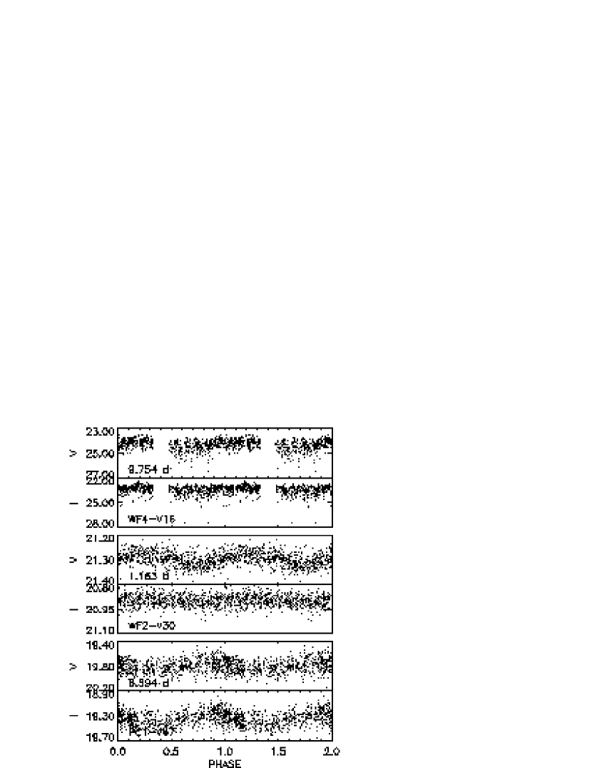
Figure 23: Phased lightcurves for three miscellaneous periodic variables.

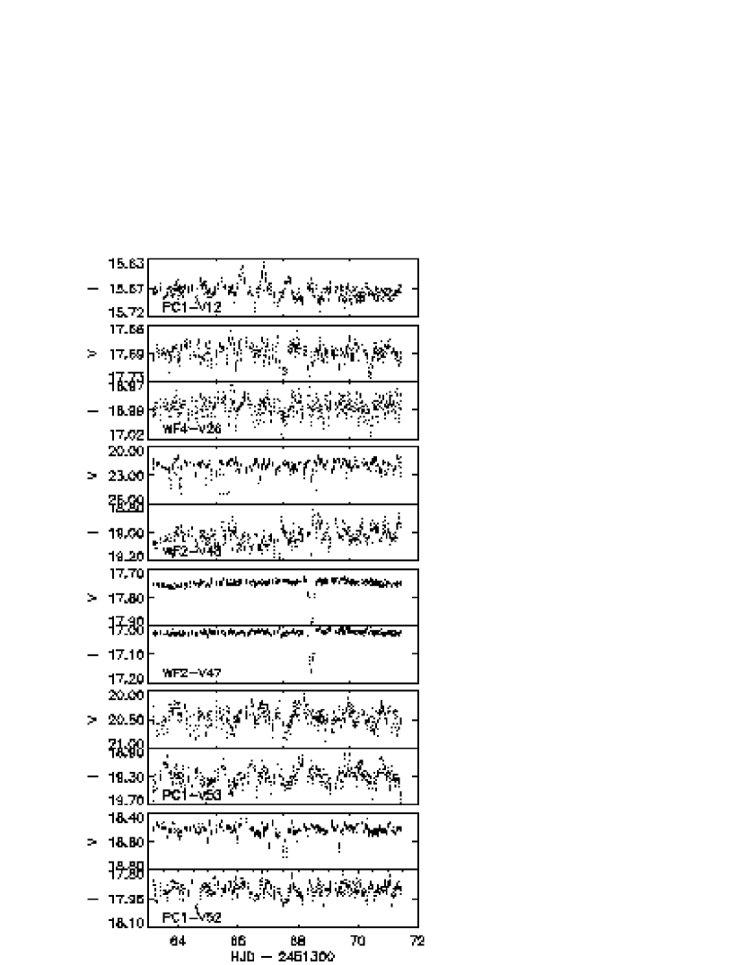
Figure 24: Lightcurves for miscellaneous irregular variables.

A small number of stars that do not fit into any of the categories considered were also found to be variable. These are listed in Table 6 and their lightcurves shown in Figs 23 and 24. The three periodic variables (PC1-V47, WF2-V30, WF4-V16; Fig 23) are the blue stars we excluded from the BY Dra sample in §7. These are candidates for being long period cataclysmic variables. WF2-V47 is an eclipsing binary which showed only one eclipse during the time of our observations. PC1-V12 is a blue straggler whose variability amplitude seemed to grow and then decline during the time we observed it. (Unfortunately this star was saturated in $V$ and attempts at $V$-band photometry were unsuccessful.) The remaining four stars (PC1-V52, PC1-V53, WF2-V48, WF4-V26) have irregular lightcurves. PC1-V53 and WF2-V48 have rather blue $U-V$ colors and WF2-V48 is also unusually red in $V-I$. We caution that WF2-V48 lies on or very close to a diffraction spike from a nearby bright star, which may have influenced the photometry. PC1-V52 lies blueward of the main sequence in $V-I$. These stars are also candidate cataclysmic variables.

9 Giant stars

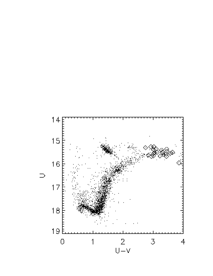
Figure 25: Color–magnitude diagram from the saturated–star photometry for all four CCDs with the variable stars indicated.

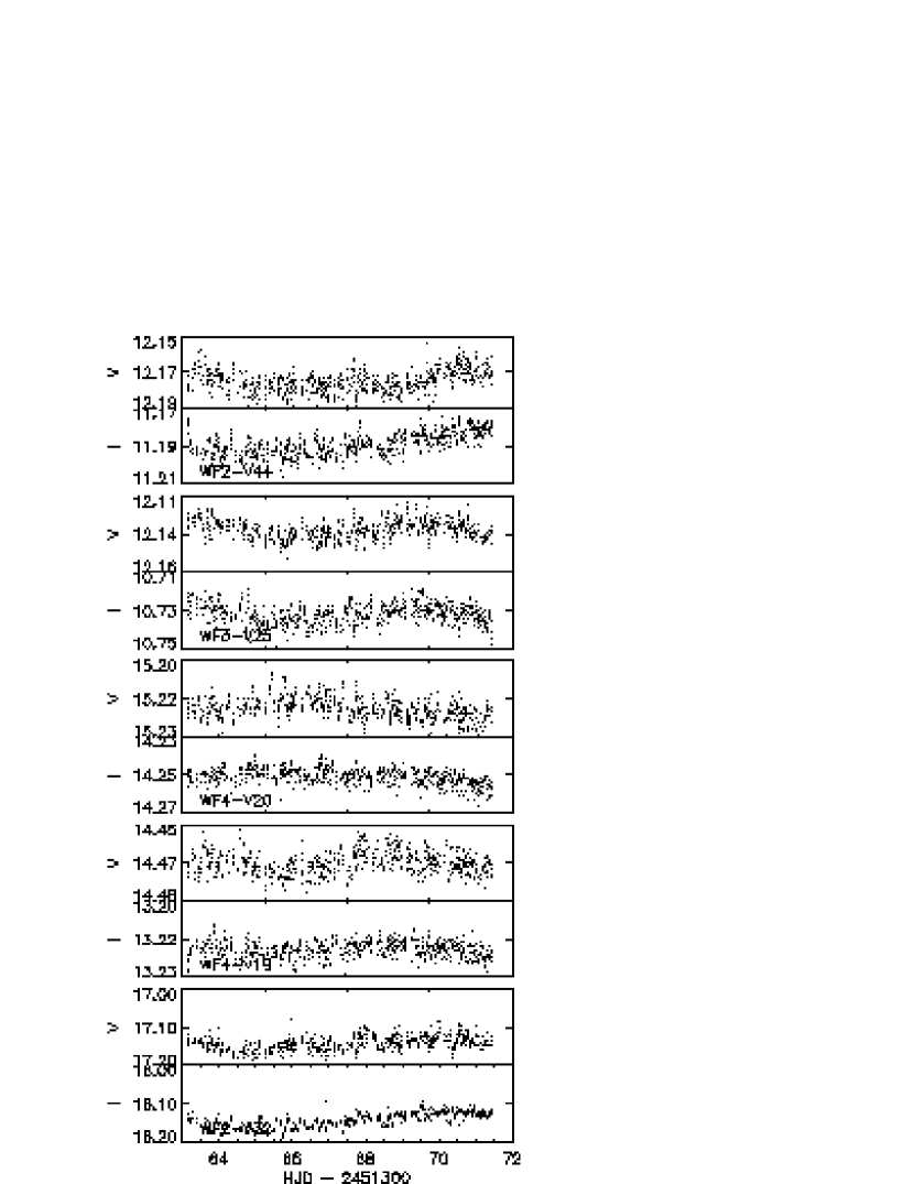
Figure 26: Sample lightcurves of variable red giants (WF2-V32, WF4-V19, WF4-V20) and RGB-AGB stars (WF3-V25, WF2-V44) from saturated-star photometry.

Using the methods of Gilliland (1994), time series photometry for $\sim$3000 saturated stars have been extracted. The quality of this photometry is not as good (typical errors of 1 – 3%) as for the unsaturated stars and the errors are not likely to be normally distributed. Nevertheless, we have searched these time series for stellar variability using the same methods and criteria as for the unsaturated stars and have found 27 giant stars which appear to be periodic variables (Tables 7 and 8). (The noise level and its time-correlated non-Gaussian characteristics meant that the saturated photometry was insensitive to detecting the $\lesssim$ 1% amplitude variables with several-day periods discussed in Edmonds & Gilliland (1996).) The distribution of the identified variables in the color–magnitude diagram is shown in Fig. 25. Since the most strongly saturated stars have extremely poor $I$–band photometry, we show this diagram in $U$, $U-V$ rather than $V$, $V-I$. The three least-saturated of these stars are also plotted in Fig. 20. Two stars, WF4-V19 and WF4-V20 (Table 7, which we label RGB), are giant-branch stars with $V$–magnitudes fainter than the horizontal branch. They may be RS CVn systems. One star, WF2-V32 at $V$ = 17.14, $V-I$ = 0.96, is located in the red straggler domain discussed in the previous section. The remaining 24 stars (Table 8, labeled RGB-AGB) are all $\sim$2 magnitudes brighter in $V$ than the horizontal branch. Most of them are probably pulsating semi-regular variables (Frogel & Whitelock, 1998) and the periods we have found from the Fourier analysis are likely underestimates. Lightcurves are shown in Fig. 26 for the two red giants, the red-straggler star and two of the RGB-AGB stars.

10 Summary

From an 8.3–day photometric campaign on the core of 47 Tucanae using WFPC2 on the Hubble Space Telescope, we have for the first time searched for variability among the main sequence stars from the cluster turnoff at $V=17$ down to magnitudes as faint as $V=25$. A total of 114 variable stars were found out of the 46422 non-saturated stars considered.

A total of 11 detached eclipsing binaries were detected, thus the observed frequency of these stars is 0.02%. Additionally we detected 15 W UMa stars corresponding to an observed frequency of 0.03%. If the angular momentum loss scenario is correct, and the distribution of binaries with log period is flat, this results in two independent estimates of 13% and 14% for the main-sequence binary frequency in the cluster core based on the detached eclipsing binaries and on the W UMa’s respectively.

Ten low-amplitude, short-period variables were identified that we assume to be the non-eclipsing counterparts of the W UMa stars.

A further 65 new variable stars have been found that are most likely BY Dra stars in binary systems. These stars are much more strongly concentrated towards the core of the cluster than single stars and follow the same spatial distribution as other binary stars.

We identify a distinct class of variables, the red stragglers, found in the (V,V-I) color-magnitude diagram slightly below and extending redwards from the subgiant branch. Six of these stars were found in our survey. We propose that these may be binary systems in which the more massive component is losing a small amount of mass to its companion or out of the system after reaching the subgiant stage of its evolution.

Figure 2: Excess “model” noise in the photometric time series. Top panel: histogram of RMS time series variations for stars with $17<V<19$ on PC1. Known variable stars have been excluded. Lower panel: Excess noise in the time series of variable stars in the same magnitude range after subtraction (in quadrature) of the mean RMS of the non-variable sample. The dotted line represents the upper envelope of such noise for non-variables.

Figure 3: The completeness of the area coverage of our survey as a function of radial distance from the center of 47 Tuc.

Figure 4: Recovery rate of simulated variables as a function of period, $V$-magnitude and signal amplitude for PC1 (left) and WF2 (right).

Figure 5: Fraction of recovered variables with periods correct to within 10% as a function of period, signal-amplitude and $V$-magnitude for PC1 (left) and WF2 (right).

Figure 8: Number of detectable eclipsing binaries vs binary fraction of the cluster. Indicated is the observed number of eclipsing binaries and its statistical error.

Figure 9: Cumulative distributions with period of the expected and observed eclipsing binaries. The solid curved line is the flat model and the dashed line the exponential model of Duquennoy & Mayor (1991). The dotted stepped line represents the observed periods.

Figure 13: Distance modulus of the 14 W UMa and near-contact binaries according to the calibration of Rucinski (1995). The eight stars consistent with being in full contact are shown with diamonds (Group 1 in text), triangles (Group 2) indicate likely semi-detached systems.

Figure 14: Color-magnitude diagram of the W UMa variables. The solid line is the fiducial main sequence ridge line of all the photometered stars. The dashed line is this line shifted upwards by 0.75 mag, i.e. the equal-mass binary main sequence. Symbols are as in Fig. 13

Figure 15: The period-luminosity diagram for the W UMa variables. Shown are lines representing equal-mass Roche-lobe filling and primary and secondary Roche-lobe filling for a binary with mass ratio $q=0.61$. Dotted parts of the curves were calculated using isochrones we have extrapolated to lower mass. Symbols are as in Fig. 13

Figure 16: Distance modulus of the short-period non-eclipsing variables according to the calibration of Rucinski (1995). Stars are plotted assuming their rotation periods are twice the observed periods. Probable contact or semi-detached systems are plotted as diamonds. Circles represent a longer-period group of stars which are probably not in or close to contact. Arrows indicate the positions of the longer period group if their observed periods are the periods of rotation, in which case near-contact conditions hold.

Figure 18: The period-luminosity diagram for the short-period non-eclipsing variables. Shown are lines representing equal-mass Roche-lobe filling and primary and secondary Roche-lobe filling for a binary with mass ratio $q=0.61$. Symbols are as in Fig. 16. Arrows show possible locations for cases in which a factor of two rotation-period abiguity remains.

Figure 20: Color-magnitude diagram of the suspected BY Dra variables. The solid line is the fiducial ridge line for 47 Tuc. The dashed line is this line shifted upwards by 0.75 mag, i.e. the equal-mass binary main sequence. Symbols are: diamonds, suspected BY Dra stars; triangles, variables from saturated-star photometry; filled circle, PC1-V11 (a known cataclysmic variable). The box near $V=17.5$ outlines the proposed red straggler domain (see text § 7.1).

Figure 22: The distribution of semi-amplitudes of the BY Dra variables (diamonds) eclipsing binaries outside of eclipse (crosses) and red straggler stars (plus signs).

Table 1: Eclipsing binaries. Phase is the epoch of primary minimum, HJD - 2451300

Name	Period (d)	Phase (d)	$V$	$U$–$V$	$V$–$I$	$\alpha$	$\delta$
PC1-V17	1.128	65.920	18.994	1.068	0.992	00:24:09.2475	-72:05:04.546
WF2-V01	10.15	70.87	20.553	2.760	1.442	00:24:05.8876	-72:04:24.816
WF2-V02	3.97	67.96	22.137	1.738	2.525	00:24:04.8394	-72:04:04.308
WF2-V03	1.340	65.442	16.194	0.402	0.550	00:24:15.4294	-72:04:41.234
WF3-V01	0.4174	65.703	19.985	1.582	1.139	00:24:19.1672	-72:04:31.339
WF3-V02	2.31	67.22	21.297	2.734	1.672	00:24:30.4310	-72:04:46.812
WF4-V01	8.87	63.53	19.276	1.503	1.043	00:24:04.7093	-72:06:08.576
WF4-V02	4.19	65.62	20.384	1.663	1.281	00:24:11.8666	-72:05:07.737
WF4-V03	0.5875	65.682	19.147	0.899	0.931	00:24:18.4695	-72:06:02.872
WF4-V04	4.92	64.85	17.129	0.669	0.778	00:24:08.2956	-72:05:35.004

Table 2: W UMa binaries

Name	Period (d)	$V$	$U$–$V$	$V$–$I$	$\alpha$	$\delta$	classification
PC1-V04	0.3301	17.523	0.479	0.668	00:24:07.5247	-72:04:58.241	contact
PC1-V07	0.4188	18.857	1.012	0.886	00:24:04.9480	-72:04:51.168	semi-detached
PC1-V08	0.5305	18.383	0.812	0.842	00:24:03.1840	-72:05:05.123	semi-detached
PC1-V10	0.4309	16.761	0.324	0.502	00:24:07.6423	-72:05:01.828	semi-detached
PC1-V18	0.2956	17.596	0.725	0.770	00:24:07.0787	-72:05:04.067	contact
PC1-V19	0.4145	20.137	1.819	1.199	00:24:04.0533	-72:05:01.221	semi-detached
PC1-V20	0.2114	22.805	1.808	1.907	00:24:06.3777	-72:04:49.255	contact
WF2-V04	0.2234	19.250	1.304	1.014	00:24:09.5679	-72:03:47.627	contact
WF2-V05	0.2021	20.184	1.959	1.212	00:24:10.6619	-72:03:52.601	contact
WF2-V06	0.3747	20.001	0.892	0.905	00:24:06.0725	-72:04:16.835	semi-detached
WF2-V07	0.2907	16.654	1.051	0.841	00:24:09.7762	-72:04:51.612	semi-detached
WF3-V03	0.3311	17.532	0.403	0.683	00:24:15.0189	-72:04:56.576	contact
WF3-V04	0.2516	18.852	0.914	0.924	00:24:18.3647	-72:04:55.203	contact
WF3-V05	0.3450	17.040	0.386	0.626	00:24:24.9261	-72:05:07.236	contact
WF4-V05	0.2588	18.643	0.122	0.131	00:24:14.6191	-72:05:40.371	semi-detached

Table 3: Non-eclipsing contact and semi-detached binaries

Name	Period (d)	$V$	$U$–$V$	$V$–$I$	$\alpha$	$\delta$	classification
PC1-V21	0.3916	21.143	2.414	1.387	00:24:05.3106	-72:04:56.160	semi-detached
PC1-V36	0.3972	17.653	0.247	0.111	00:24:06.2184	-72:04:52.168	semi-detached
PC1-V46	0.2656	17.785	0.589	0.651	00:24:05.7776	-72:04:49.139	contact
WF2-V08	0.4011	21.277	-1.875	-0.280	00:24:15.1166	-72:03:36.569	semi-detached
WF2-V09	0.2405	20.137	-1.246	0.396	00:24:16.7173	-72:04:27.124	semi-detached
WF3-V06	0.2316	22.929	0.500	0.697	00:24:25.4577	-72:04:38.204	semi-detached
WF3-V07	0.3163	19.597	-0.066	-0.060	00:24:14.2860	-72:04:54.745	semi-detached
WF3-V08	0.2108	20.832	2.853	1.202	00:24:15.7319	-72:04:51.695	semi-detached
WF3-V09	0.3311	19.022	0.723	0.782	00:24:11.9652	-72:05:00.108	semi-detached
WF3-V10	0.3325	17.120	0.639	0.732	00:24:13.3209	-72:05:06.947	contact

Table 4: BY Draconis variables. $A_{V}$ is the $V$-band semi-amplitude (mag).

Name	Period (d)	$A_{V}$	$V$	$U$–$V$	$V$–$I$	$\alpha$	$\delta$
PC1-V22	2.50	0.012	17.839	0.633	0.724	00:24:04.7693	-72:04:56.028
PC1-V23	4.36	0.030	16.985	0.593	0.791	00:24:06.0691	-72:04:52.698
PC1-V24	2.43	0.024	17.363	0.589	0.764	00:24:06.9408	-72:04:57.384
PC1-V25	1.03	0.022	20.849	1.891	1.139	00:24:06.5582	-72:04:55.926
PC1-V26	2.43	0.005	17.653	0.462	0.713	00:24:06.4777	-72:04:46.016
PC1-V27	4.03	0.009	18.121	0.552	0.718	00:24:08.4830	-72:05:00.408
PC1-V28	1.16	0.036	20.135	1.351	1.017	00:24:04.6105	-72:04:59.546
PC1-V29	0.528	0.038	21.136	2.206	1.402	00:24:07.8785	-72:05:13.195
PC1-V30	0.798	0.015	19.279	1.079	1.073	00:24:03.8530	-72:05:12.300
PC1-V31	4.35	0.024	19.334	1.013	0.947	00:24:06.8886	-72:04:48.795
PC1-V32	1.64	0.008	18.858	0.910	0.792	00:24:05.4040	-72:04:52.316
PC1-V33	1.74	0.011	19.075	0.880	0.952	00:24:06.6562	-72:04:44.424
PC1-V34	1.38	0.017	20.382	1.744	1.118	00:24:06.9072	-72:04:52.677
PC1-V35	4.86	0.004	17.695	0.498	0.779	00:24:06.7297	-72:04:42.026
PC1-V37	4.86	0.010	19.283	1.255	1.045	00:24:04.2535	-72:04:56.922
PC1-V38	6.89	0.007	19.285	1.271	1.008	00:24:05.9036	-72:04:57.097
PC1-V39	4.73	0.005	18.435	0.725	0.757	00:24:04.9713	-72:05:00.590
PC1-V40	4.47	0.005	18.569	0.944	0.887	00:24:05.6368	-72:04:53.466
PC1-V41	5.02	0.002	17.625	0.867	0.704	00:24:08.4775	-72:05:07.420
PC1-V42	0.521	0.015	21.170	1.634	1.335	00:24:01.7154	-72:05:01.649
PC1-V43	5.16	0.003	18.933	0.839	0.924	00:24:06.5748	-72:04:44.095
WF2-V10	9.18	0.009	17.487	0.553	0.776	00:24:15.5759	-72:04:33.326
WF2-V11	0.843	0.074	20.025	1.299	1.044	00:24:13.7868	-72:04:02.830
WF2-V12	1.18	0.061	19.437	1.059	1.000	00:24:13.2504	-72:04:47.190
WF2-V13	5.93	0.005	18.066	0.444	0.713	00:24:13.2992	-72:04:36.197
WF2-V14	4.14	0.004	17.986	0.476	0.714	00:24:08.1418	-72:04:26.200
WF2-V15	1.29	0.007	18.192	0.642	0.700	00:24:10.8166	-72:04:43.935
WF2-V16	1.74	0.037	21.491	2.472	1.660	00:24:14.9671	-72:03:32.018
WF2-V17	0.633	0.003	17.338	0.463	0.753	00:24:06.2042	-72:04:30.219
WF2-V18	3.06	0.014	18.312	0.872	0.936	00:24:12.3851	-72:04:22.230
WF2-V19	1.56	0.033	21.188	2.083	1.682	00:24:07.0542	-72:04:14.252
WF2-V20	2.58	0.049	20.886	2.162	1.391	00:24:04.5152	-72:03:56.537
WF2-V21	1.50	0.023	20.800	2.184	1.428	00:24:09.7754	-72:04:26.184
WF2-V22	0.549	0.054	20.713	1.325	1.603	00:24:06.8901	-72:04:20.155
WF2-V23	7.20	0.008	18.894	1.313	0.871	00:24:12.2897	-72:04:11.555
WF2-V24	6.39	0.006	17.966	0.425	0.659	00:24:15.1099	-72:04:23.037
WF2-V25	6.62	0.004	17.712	0.400	0.678	00:24:04.8793	-72:04:24.885
WF2-V26	5.70	0.007	20.312	1.091	1.107	00:24:22.4470	-72:04:05.321
WF2-V27	2.47	0.003	18.024	0.636	0.793	00:24:05.7002	-72:04:18.673
WF2-V28	6.39	0.004	19.265	0.954	0.889	00:24:14.5934	-72:04:05.350
WF2-V29	3.76	0.002	17.547	0.405	0.700	00:24:11.1291	-72:04:40.100
WF3-V11	7.20	0.003	17.468	0.624	0.715	00:24:14.4423	-72:05:05.259
WF3-V12	1.78	0.006	17.479	0.493	0.722	00:24:16.4839	-72:04:47.005
WF3-V13	1.99	0.003	17.582	0.448	0.700	00:24:22.8584	-72:05:31.781
WF3-V14	5.16	0.028	19.669	1.262	1.033	00:24:21.0290	-72:05:02.810
WF3-V15	0.437	0.023	20.294	1.917	1.415	00:24:24.3744	-72:05:00.255
WF3-V16	2.50	0.010	19.257	1.066	0.954	00:24:14.7970	-72:05:02.997
WF3-V17	7.89	0.011	19.875	1.410	0.953	00:24:21.7737	-72:04:25.483
WF3-V18	5.70	0.008	19.728	1.388	0.921	00:24:26.8360	-72:05:25.692
WF3-V19	1.88	0.041	22.996	0.254	1.975	00:24:28.6891	-72:05:00.584
WF3-V20	7.57	0.013	21.514	2.808	1.585	00:24:19.8193	-72:05:25.453
WF3-V21	4.03	0.015	21.420	2.867	1.998	00:24:18.5850	-72:05:04.426
WF3-V22	0.893	0.010	20.764	3.050	1.501	00:24:15.0728	-72:04:49.656
WF3-V23	9.75	0.001	17.501	0.474	0.670	00:24:16.0377	-72:04:59.281
WF3-V24	7.89	0.020	22.160		1.714	00:24:24.5505	-72:04:53.861
WF4-V06	6.13	0.031	17.120	0.505	0.735	00:24:10.2673	-72:05:06.501
WF4-V07	1.44	0.026	19.894	1.173	1.138	00:24:12.2932	-72:05:21.804
WF4-V08	2.04	0.013	20.670	2.291	1.462	00:24:07.2830	-72:06:19.875
WF4-V09	1.37	0.019	20.743	2.111	1.270	00:24:07.4045	-72:05:53.703
WF4-V10	2.62	0.007	19.767	2.320	1.324	00:24:06.3807	-72:05:42.025
WF4-V11	8.72	0.016	20.604	1.865	1.142	00:24:14.9759	-72:05:29.017
WF4-V12	6.13	0.004	17.624	0.461	0.650	00:24:04.5026	-72:05:37.311
WF4-V13	9.18	0.013	20.911		1.297	00:24:13.0519	-72:06:04.108
WF4-V14	4.35	0.004	18.180	0.640	0.730	00:24:09.5175	-72:06:00.822
WF4-V15	0.903	0.028	21.813		1.734	00:24:08.1056	-72:06:21.536

Table 5: Red Straggler variables

Name	Period (d)	$A_{V}$	$V$	$U$–$V$	$V$–$I$	$\alpha$	$\delta$
PC1-V11	1.108	0.117	17.391	0.287	0.941	00:24:04.6452	-72:04:55.300
PC1-V48	6.71	0.005	17.386	1.147	0.989	00:24:10.1782	-72:04:59.780
WF2-V31	5.34	0.073	17.576	1.301	1.139	00:24:14.9180	-72:04:43.454
WF2-V32	9.2	0.011	17.141	1.013	0.997	00:24:13.5415	-72:03:34.452
WF4-V17	4.86	0.003	17.567	2.573	1.294	00:24:11.5517	-72:06:31.694
WF4-V18	5.90	0.020	17.277	0.769	0.870	00:24:11.7456	-72:05:12.414

Table 6: Other variables

Name	Period (d)	$V$	$U$–$V$	$V$–$I$	$\alpha$	$\delta$
PC1-V12		16.076	0.318	0.397	00:24:06.1630	-72:04:45.264
PC1-V47	6.39	19.772	-0.904	0.456	00:24:03.9773	-72:04:57.885
PC1-V52		18.514	0.561	0.615	00:24:05.9771	-72:04:45.979
PC1-V53		20.411	-1.028	1.138	00:24:05.7208	-72:04:56.015
WF2-V30	1.16	21.295	-1.624	0.400	00:24:14.8416	-72:03:44.793
WF2-V47		17.750	1.247	0.725	00:24:08.2107	-72:04:27.204
WF2-V48		21.677	-0.434	2.657	00:24:15.6337	-72:04:36.312
WF4-V16	9.75	24.070		0.918	00:24:04.6068	-72:06:05.958
WF4-V26		17.694	0.571	0.702	00:24:14.5067	-72:05:59.154

Table 7: Variable giants

Name	Period (d)	$V$	$U$–$V$	$V$–$I$	$\alpha$	$\delta$
WF4-V19	5.9	14.465	1.865	1.246	00:24:07.5500	-72:05:20.097
WF4-V20	$>$10	15.219	1.377	0.968	00:24:10.9840	-72:05:08.778

Table 8: Variable RGB-AGB stars

Name	Period (d)	$V$	$U$–$V$	$V$–$I$	$\alpha$	$\delta$
PC1-V49	7.51	12.152	3.435	1.440	00:24:08.4012	-72:05:11.301
PC1-V50	7.2	12.108	3.857	1.364	00:24:10.5132	-72:05:02.312
WF2-V33	6.36	12.341	2.930	0.730	00:24:03.4806	-72:04:17.984
WF2-V34	5.5	12.266	3.341	1.203	00:24:08.1873	-72:04:35.784
WF2-V35	5.7	12.238	3.025		00:24:14.4012	-72:04:27.294
WF2-V36	2.85	12.789	2.841		00:24:01.6237	-72:04:04.320
WF2-V37	6.5	12.245	3.437		00:24:13.0092	-72:03:55.552
WF2-V38	9	11.214	3.640		00:24:14.5151	-72:04:44.337
WF2-V39	6.1	12.432	3.230		00:24:12.5795	-72:03:38.357
WF2-V40	9	12.011	3.451		00:24:01.6279	-72:04:09.160
WF2-V41	6.6	12.195	3.313		00:24:07.5314	-72:04:23.170
WF2-V42	$>$10	11.868	3.642		00:24:11.3878	-72:03:25.178
WF2-V43	5.9	12.558	2.748		00:24:10.3531	-72:04:40.807
WF2-V44	$>$10	12.175	3.287		00:24:17.0016	-72:04:30.134
WF2-V45	5	12.264	3.100		00:24:06.5038	-72:04:25.938
WF2-V46	3.5	12.648	3.008		00:24:13.5246	-72:04:28.373
WF3-V25	6.1	12.132	3.278	1.400	00:24:28.5997	-72:04:42.486
WF3-V26	9	11.919	3.449	1.534	00:24:13.4766	-72:04:52.361
WF3-V27	7.5	11.962	3.579	1.484	00:24:19.0539	-72:05:18.956
WF4-V21	7	12.383	3.016	1.699	00:24:09.9840	-72:05:33.961
WF4-V22	5	12.477	3.046	1.585	00:24:20.0184	-72:05:51.770
WF4-V23	3.9	12.530	3.018	1.353	00:24:06.6003	-72:06:15.451
WF4-V24	9	12.741	2.944	1.271	00:24:11.0310	-72:05:35.552
WF4-V25	$>$10	12.387	3.126	1.605	00:24:20.2301	-72:05:58.480

References

- Alard (1999) Alard C., 1999, A&A, 343, 10
- Alcaino, & Liller (1987) Alcaino, G., & Liller, W., 1987, ApJ, 319, 304
- Alcock et al. (1999) Alcock, C. et al., 1999, ApJ, 521, 602
- Bacon, Sigurdsson, & Davies (1996) Bacon, D., Sigurdsson, S., & Davies, M.B., 1996, MNRAS, 281, 830
- Belloni, Verbunt, & Mathieu (1998) Belloni, T., Verbunt, F., & Mathieu, R.D. 1998, A&A, 1998, 339, 431
- Bertelli et al. (1994) Bertelli, G., Bressan, A., Chiosi, C., Fagotto, F., & Nasi, E., 1994, A&AS, 106, 275
- Bopp & Evans (1973) Bopp, B.W., & Evans, D.S., 1973, MNRAS, 164, 343
- Bopp & Fekel (1977) Bopp, B.W., & Fekel, F., 1977, AJ, 82, 490
- Bradstreet & Guinan (1994) Bradstreet, D.H., & Guinan, E.F., 1994, in ASP Conf. Ser. 56, Interacting Binary Stars, ed. A.W. Shafter (San Francisco:ASP), 228
- Callanan, Penny, & Charles (1995) Callanan, P.J., Penny, A.J., & Charles, P.A., 1995, MNRAS, 273, 201
- Camilo et al. (2000) Camilo, F., Lorimer, D.R., Freire, P., Lyne, A.G., & Manchester, R.N., 2000, ApJ, 535, 975
- Cutispoto (1993) Cutispoto, G., 1993, A&AS, 102, 655
- D’Amico et al. (2001) D’Amico, N., Lyne, A.G., Manchester, R.N., Possenti, A., & Camilo, F., 2001, ApJ, 548, 171
- Davies (1995) Davies, M.B., 1995, MNRAS, 276, 887
- Dempsey et al. (1997) Dempsey, R.C., Linsky, J.L., Fleming, T.A., & Schmitt, J.H.M.M., 1997, ApJ, 478, 358
- Duquennoy & Mayor (1991) Duquennoy, A., & Mayor, M., 1991, A&A, 248, 485
- Edmonds & Gilliland (1996) Edmonds, P.D., & Gilliland, R.L., 1996, ApJ, 464, 157
- Edmonds et al. (1996) Edmonds, P.D., Gilliland, R.L., Guhathakurta, P., Petro, L.D., Saha, A., & Shara, M.M., 1996, ApJ, 468, 241
- Edmonds et al. (1999) Edmonds, P.D., Grindlay, J.E., Cool, A., Cohn, H., Lugger, P., & Bailyn, C., 1999, ApJ, 516, 250
- Eggen & Iben (1989) Eggen, O.J., & Iben, I. Jr, 1989, AJ, 97, 431
- Eggleton (1983) Eggleton, P.P., 1983, ApJ, 268, 368
- Elson et al. (1988) Elson, R.A.W., Sigurdsson, S., Davies, M., Hurley, J., & Gilmore, G., 1998, MNRAS, 300, 857
- Flannery (1976) Flannery, B.P., 1976, ApJ, 205, 217
- Frogel & Whitelock (1998) Frogel, J.A., & Whitelock, P.A., 1998, AJ, 116, 754
- Gilliland (1982) Gilliland, R.L. 1982, ApJ, 263, 302
- Gilliland (1985) Gilliland, R.L. 1985, ApJ, 299, 286
- Gilliland et al. (1991) Gilliland, R.L., et al., 1991, AJ, 101, 541
- Gilliland (1994) Gilliland, R.L., 1994, ApJ, 435, L63
- Gilliland et al. (1998) Gilliland, R.L., Bono, G., Edmonds, P.D., Caputo, F., Cassisi, S., Petro, L.D., Saha, A., & Shara, M.M., 1998, ApJ, 507, 818
- Gilliland et al. (2000) Gilliland, R.L., et al., 2000, ApJ, 545, L47
- Goodman & Hut (1993) Goodman, J., & Hut, P., 1993, ApJ, 403, 271
- Guhathakurta et al. (1992) Guhathakurta, P., Yanny, B., Schneider, D.P., & Bahcall, J.N., 1992, AJ, 104, 1790
- Harris (1996) Harris, W.E., 1996, AJ, 112, 1487
- Heggie (1975) Heggie, D.C., 1975, MNRAS, 173, 729
- Heggie & Aarseth (1992) Heggie, D.C., & Aarseth, S.J., 1992, MNRAS, 257, 513
- Heggie, Hut, & McMillan (1996) Heggie, D.C., Hut, P., & McMillan, S.L.W., 1996, ApJ, 467, 359
- Hesser et al. (1987) Hesser, J.E., Harris, W.E., Vandenberg, D.A., Allwright, J.W.B., Shott, P., & Stetson, P.B., 1987, PASP, 99, 739
- Hills (1975) Hills, J.G., 1975, AJ, 80, 809
- Hills (1984) Hills, J.G., 1984, AJ, 89, 1811
- Hills (1992) Hills, J.G., 1992, AJ, 103, 1955
- Holtzman et al. (1995) Holtzman, J.A., Burrows, C.J., Casertano, S., Hester, J.J., Trauger, J.T., Watson, A.M., & Worthey, G. 1995, PASP, 107, 1065
- Howell, Guhathakurta, & Gilliland (2000) Howell, J.H., Guhathakurta, P., & Gilliland, R.L., 2000, PASP, 112, 1200
- Hut et al. (1992) Hut, P., et al., 1992, PASP, 104, 981
- Iben & Livio (1993) Iben, I. Jr, & Livio, M., 1993, PASP, 105, 1373
- Kaluzny & Krzeminski (1993) Kaluzny, J., & Krzeminski, W., 1993, MNRAS, 264, 785
- Kaluzny et al. (1996) Kaluzny, J., Kubiak, M., Szymanski, M., Udalski, A., Krzeminski, W., & Mateo, M., 1996, A&AS, 120, 139
- Kaluzny (1997) Kaluzny, J., 1997, A&AS, 122, 1
- Kaluzny, Thompson, & Krzeminski (1997) Kaluzny, J., Thompson, I.B., & Krzeminski, W., 1997, AJ, 113, 2219
- Kaluzny et al. (1997a) Kaluzny, J., Krzeminski, W., Mazur, B., Wysocka, A., & Stepien, K., 1997a, Acta Astronomica, 47, 249
- Kaluzny et al. (1997b) Kaluzny, J., Kubiak, M., Szymanski, M., Udalski, A., Krzeminski, W., Mateo, M., & Stanek, K., 1997b, A&AS, 122, 471
- Kaluzny et al. (1998a) Kaluzny, J., Kubiak, M., Szymanski, M., Udalski, A., Krzeminski, W., Mateo, M., & Stanek, K., 1998a, A&AS, 128, 19
- Kaluzny et al. (1998b) Kaluzny, J., Wysocka, A., Stanek, K.Z., & Krzeminski, W., 1998b, Acta Astronomica, 48, 439
- Keppens (1997) Keppens, R. 1997, A&A, 318, 275
- Keppens, Solanki, & Charbonnel (2000) Keppens, R., Solanki, S.K., & Charbonnel, C. 2000, A&A, 359, 552
- Knigge et al. (2000) Knigge, C., Shara, M.M., Zurek, D.R., Long, K.S., & Gilliland, R.L., 2000, preprint, astro-ph/0012187
- Mathieu, Walter, & Myers (1989) Mathieu, R.D., Walter, F.M., & Myers, P.C., 1989, AJ, 98, 987
- Mathieu (1994) Mathieu, R.D., 1994, ARA&A, 32, 465
- Mathieu et al. (2000) Mathieu, R.D., Latham, D.W., Stassun, K.G., Torres, G., van den Berg, M., & Verbunt, F., 2000, AAS, 197, 4111.
- McMillan & Hut (1996) McMillan, S.L.W., & Hut, P., 1996, ApJ, 467, 348
- Menzies, O’Donaghue, & Warner (1986) Menzies, J.W., O’Donaghue, D., & Warner, B., 1986, Ap&SS, 122, 73
- Meylan & Mayor (1986) Meylan, G., & Mayor, M., 1986, A&A, 166, 122
- Meylan & Heggie (1997) Meylan, G., & Heggie, D.C., 1997, A&A Rev., 8, 1
- Paczynski (1971) Paczynski, B., 1971, ARA&A, 9, 183
- Portegies Zwart et al. (1997) Portegies Zwart, S.F., Hut, P., McMillan, S.L.W., & Verbunt, F., 1997 A&A, 328, 143
- Press et al. (1992) Press, W.H., Teukolsky, S.A., Vetterling, W.T., & Flannery, B.P., 1992, Numerical Recipes in C, 2nd Edition (Cambridge:Cambridge University Press)
- Rahunen (1981) Rahunen, T., 1981, A&A, 102, 81
- Robertson & Eggleton (1977) Robertson, J.A., & Eggleton, P.P., 1977, MNRAS, 179, 359
- Rubenstein & Bailyn (1996) Rubenstein, E.A., & Bailyn, C.D., 1996, AJ, 111, 260
- Rubenstein & Bailyn (1997) Rubenstein, E.A., & Bailyn, C.D., 1997, ApJ, 474, 701
- Rucinski (1994) Rucinski, S.M., 1994, PASP, 106, 462
- Rucinski (1995) Rucinski, S.M., 1995, PASP, 107, 648
- Rucinski (1997) Rucinski, S.M., 1997, AJ, 113, 407
- Rucinski (2000) Rucinski, S.M., 2000, AJ, 120, 319
- Scargle (1982) Scargle J.D., 1982, ApJ, 263, 835
- Schlegel et al. (1998) Schlegel D.J., Finkbeiner D.P., Davis M., 1998, ApJ, 500, 525
- Shara et al. (1988) Shara, M.M., Kaluzny, J., Potter, M., & Moffat, A.F.J., 1988, ApJ, 328, 594
- Shara, Saffer, & Livio (1997) Shara, M.M., Saffer, R.A., & Livio, M., 1997, ApJ, 489, L59
- Siess & Livio (1997) Siess, L., & Livio, M., 1997, ApJ, 490, 785
- Sigurdsson & Phinney (1995) Sigurdsson, S., & Phinney, E.S., 1995, ApJS, 99, 609
- Skumanich (1972) Skumanich, A., 1972, ApJ, 171, 565
- Soderblom (1983) Soderblom, D.R., 1983, ApJS, 53, 1
- Soderblom (1990) Soderblom, D.R. 1990, AJ, 100, 204
- Stetson (1987) Stetson, P.B., 1987, PASP, 99, 191
- Stetson (1992) Stetson, P.B., 1992, in ASP Conf. Ser. 25, Astronomical Data Analysis Software, ed., D.M. Worrell, G. Biemsdorfer, J. Bernas (San Francisco:ASP), 297
- VandenBerg (2000) VandenBerg, D.A. 2000, ApJS, 129, 315
- VandenBerg, Verbunt, & Mathieu (1999) VandenBerg, M., Verbunt, F., & Mathieu, R.D. 1999, A&A, 347, 866
- Vilhu (1982) Vilhu, O., 1982, A&A, 109, 17
- Vogt, Penrod, & Soderblom (1983) Vogt, S.S., Penrod, G.D., & Soderblom, D.R. 1983, ApJ, 269, 250
- Whitmore, Heyer, & Casertano (1999) Whitmore, B., Heyer, I., & Casertano, S., 1999, PASP, 111, 1559
- Yan & Mateo (1994) Yan, L., & Mateo, M., 1994, AJ, 108, 1810
- Yan & Reid (1996) Yan, L., & Reid, I.N., 1996, MNRAS, 279, 751
- Zoccali et al. (2001) Zoccali, M., et al., 2001, ApJ, in press, (astro-ph/0101485)