Search for Supernova Neutrino-Bursts with the Amanda Detector

Abstract

The core collapse of a massive star in the Milky Way will produce a neutrino burst, intense enough to be detected by existing underground detectors. The AMANDA neutrino telescope located deep in the South Pole ice can detect MeV neutrinos by a collective rate increase in all photo-multipliers on top of dark noise. The main source of light comes from positrons produced in the CC-reaction of anti-electron neutrinos on free protons $\mbox{${\bar{\nu}}_{e}$}+p\rightarrow e^{+}+n$. This paper describes the first supernova search performed on the full sets of data taken during 1997 and 1998 (215 days of live time) with 302 of the detector’s optical modules. No candidate events resulted from this search. The performance of the detector is calculated, yielding a 70$\%$ coverage of the Galaxy with one background fake per year with 90$\%$ efficiency for the detector configuration under study. An upper limit at the 90$\%$ c.l. on the rate of stellar collapses in the Milky Way is derived, yielding 4.3 events per year. A trigger algorithm is presented and its performance estimated. Possible improvements of the detector hardware are reviewed.

, , , , , , , , , , , , , , , , , , , , , , , , , , , , , , , , , , , , , , , , , , , , , , , , , , , , , , , , , , , , , , , , , , , , , , , , , , , , , , , , , , , , , , , , , , , , , , , , , , , , ,

1 Introduction

Astronomical observations have customarily been carried out by detecting photons, from radio-waves to gamma rays, with each new range of energy uncovered leading to fresh discoveries. Over the years, the electro-magnetic spectrum has been well covered, leaving no new frequency-gaps to explore.

Neutrino astronomy is still in its infancy, but it is a field which has been growing over the past few decades. Besides providing a new probe to investigate the universe, the neutrino is also fundamentally different from the photon in that it interacts only weakly and can thus still be observed after passing through large amounts of matter. This is a mixed blessing, however, since the detection of neutrinos on Earth is made more difficult by the very same reason and requires correspondingly large detector volumes. Furthermore, neutrinos remain undeflected by magnetic fields.

Until now, the only extra-terrestrial sources of neutrinos that have been observed are the Sun and the supernova SN1987A. In both cases, the energies seen were at or below a few tens of MeV. The ${\bar{\nu}}_{e}$ -burst emitted in the 1987 supernova event was detected simultaneously by the IMB [1] and Kamiokande II [2, 3] water detectors, a few hours ahead of its optical counterpart. Due to the distant location of the supernova in the Large Magellanic Cloud ($\sim$52 kpc from us), only 20 neutrinos were collected in total. This was still enough to confirm that most of the energy was released in the form of neutrinos and also to validate the essential predictions of models describing the mechanism of gravitational collapse supernovae. SN1987A proved also that relevant particle physics information can be extracted from astrophysical events. The data was used to set an upper limit on the mass of the ${\bar{\nu}}_{e}$, its lifetime, its magnetic moment and the number of leptonic flavours.

However, although the rough features in terms of energies, duration and flux were supported by the observations, they said next to nothing about the details of the burst development. For this, hundreds if not thousands of neutrinos would be needed. Furthermore, both experiments were insensitive to flavors other than ${\bar{\nu}}_{e}$, which are expected to carry away most of the supernova energy. The detection of a type II supernova in the Milky Way would provide us with a unique opportunity to study the details of the gravitational collapse of a star. Several low-energy neutrino detectors exist already (LVD, Super-Kamiokande, SNO [4] and Baksan [5]) which will be able to shed light on the core collapse of a massive star, should such an event occur during their lifetime.

Amanda (Antarctic Muon and Neutrino Detector Array [6]) is one of several high energy neutrino telescopes. Another existing detector is NT200 in lake Baikal [7], whereas others are under development (ANTARES [8], NESTOR [9] and NEMO [10]). Amanda consists of optical modules (OMs) buried 1500-2000 m deep in the Antarctic ice sheet. Each OM is made up of a photo-multiplier tube (PMT) enclosed in a pressure-resistant glass vessel and connected to the surface electronics by an electrical cable supplying power and transmitting the PMT signals.

Amanda is designed for the observation of TeV neutrino-sources, utilizing the large volume of transparent glacier ice available at the South Pole as a Cherenkov medium. In spite of the much lower neutrino energies of ${\mathcal{O}}$(10 MeV) involved in a burst, it has been shown [11] that a detector of this type could also be used successfully to monitor our Galaxy for supernova events (the description of a method for neutrino telescopes using ocean water can be found in [12]). Since the cross-section for inverse $\beta$ decay reaction on protons $\mbox{${\bar{\nu}}_{e}$}+p\rightarrow n+e^{+}$ in the ice exceeds the cross-sections for the other neutrino flavors and targets, ${\bar{\nu}}_{e}$ events are dominating . During the estimated $\sim$ 10 sec duration of a neutrino-burst, the Cherenkov light produced by the positron tracks will increase the counting rate of all the PMTs in the detector above their average value. This effect, when considered as a collective behavior, could be seen clearly even if the increase in each PMT would not be statistically significant. An observation made over a time window of several sec could therefore provide a detection of a supernova, before its optical counterpart is observed. The stable and low background noise in Amanda (absence of ${}^{40}K$ and of bioluminescence in the ice) is a clear asset for this method.

In this paper, the 302 OMs of the Amanda B10 stage completed in 1997 are used for the analysis. In the next section, we summarize the theoretical expectations for the neutrino burst which is emitted when a massive star undergoes gravitational core collapse. An account is then given of the detector hardware, as well as of the data collected with it. The analysis method is explained next and the results obtained from its application to experimental data are presented. A study of the detector performance follows. Next, the principle of an online trigger algorithm is described. We end with a discussion of possible improvements of the detector. Early searches for supernova neutrino-burst signals with the Amanda detector have been presented in [13, 14, 15].

2 Theoretical preliminaries

When the core of a massive star ($M\geq 8M_{\odot}$) runs out of nuclear fuel, it collapses and ejects the outer mantle in a SN explosion of type II/Ib/Ic  [16]. Only $\sim 1\%$ of the energy is released in kinetic and optical form, whereas the remaining $99\%$ of the gravitational binding energy change, about $3\times 10^{53}$ ergs, is carried away by neutrinos [17].

During the process, the inner core reaches nuclear densities, bringing the collapse to an abrupt stop, and a shock-wave is formed. The front of this shock is driven outward, through the in-falling material, passing through the neutrinosphere (the location where the material changes from opaque to transparent to neutrinos) on its way, until a point where it stalls .

During the first 10 msec, a $\nu_{e}$ burst from the neutronization process $e^{-}+p\rightarrow n+\mbox{$\nu_{e}$}$ releases $\sim 10^{52}$ ergs. Although neutrinos interact only weakly, the densities built up during the collapse are so high that they cannot stream out. Instead, they are trapped and diffuse out over a time scale of several sec. When they finally reach the neutrinosphere they can escape, with a thermal spectrum which is approximately Fermi-Dirac [17]. The trapped neutrinos are produced in pairs through the reaction $e^{-}+e^{+}\stackrel{{\scriptstyle Z}}{{\rightarrow}}\nu+\bar{\nu}$ for all lepton flavors. In addition, the $\nu_{e}$${\bar{\nu}}_{e}$ pairs are also produced via $p(n)+e^{-(+)}\stackrel{{\scriptstyle W}}{{\rightarrow}}n(p)+\stackrel{{\scriptstyle(-)}}{{\nu_{e}}}$. They are produced with distinctive energies, because the neutrino-spheres for each type are located at depths with different temperatures. The $\nu_{\mu}$ and $\nu_{\tau}$ and their anti-particles have a mean energy of $\left<E\right>\approx 25\rm\,MeV$. The ${\bar{\nu}}_{e}$ have a mean energy $\left<E\right>\approx 16\rm\,MeV$ and the corresponding value for $\nu_{e}$ neutrinos is $\left<E\right>\approx 11\rm\,MeV$ [18]. In total, the radiated energy is expected to be equally distributed over each flavor of neutrinos and anti-neutrinos [19]. The luminosity-profile can be described by a quick rise over a few msec and more and then falling over a time of $\mathcal{O}({\mbox{several sec}})$, roughly like an exponential with a time constant $\tau=3~{}\rm sec$ [20]. During the late phase the neutrino luminosity possibly follows a power law with index $\sim 1\pm 0.5$ [17]. The detailed form of the neutrino luminosity used below is less important than the general shape features and their characteristic durations [20].

Figure 1: The distribution $f(r)$ of progenitor stars in the Milky Way, located within a distance $r$ from the Earth. Inset: the corresponding cumulative distribution $F(r)$ (taken from a model by Bahcall & Soneira [21, 22]). The steep behavior around $\sim$ 8 kpc is due to the high star density in the Galactic bulge.

Currently, the rate of galactic stellar collapses is estimated to be one every 40 years [23], with a best experimental upper limit of 1 every 5 years [5]. At least three underground neutrino detectors (Super-Kamiokande [24], Baksan [5], LVD [25]) have a sensitivity high enough to cover the Galaxy and beyond ( the distribution of progenitor stars in the Milky Way is shown in Fig.1).

3 Description of the detector

The Amanda detector has been deployed over several years[6]. Each deployment phase consists of drilling holes in the ice and lowering strings of OMs connected to electrical cables (see Fig.2). In this text, we will limit ourselves to the study of data taken in 1997 and 1998, with ten strings (302 OMs) in operation during these two years.

The first four strings were deployed in 1995-1996, using coaxial cable. Strings 5-10 followed in 1996-1997, using twisted-pair cable. Hamamatsu photo-multipliers (PMTs) of type R5912-02 were used in all OMs. The PMTs of strings 1-4 are enclosed in spheres manufactured by Billings, whereas the remaining strings use spheres with better transparency [14], produced by Benthos company. The AMANDA-supernova detector was part of the AMANDA-SNMP (SuperNova-MonoPole) data-acquisition system (DAQ) [14], which operates independently from the AMANDA muon-trigger and DAQ. It consisted of custom-made CAMAC modules and is read out by a Macintosh via a standard SCSI interface.

The idea is to continuously measure the counting rates of all OM channels separately and store that data for further analysis. For this, each channel counted the arriving OM-pulses synchronously into a separate 12-bit counter during a fixed time interval of 500 msec which is synchronized by a GPS-clock.

Correlated noise following OM-pulses was suppressed by a common programmable dead-time in the range of 100 ns to 12.8 $\mu$s (which was set to 10 $\mu$s).

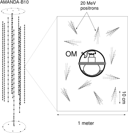
Figure 2: View of the detector and of the expected positron tracks produced in CC $\bar{\nu_{e}}$ interactions within Amanda

The present detector configuration has nine additional strings, bringing the total number of OMs to 680, and the data is currently taken with an upgraded VME/Linux based DAQ.

3.1 Low-energy ${\bar{\nu}}_{e}$ in Amanda

The anti-electron neutrinos produced in a supernova follow a Fermi-Dirac distribution with $\left<E_{\mbox{${\bar{\nu}}_{e}$}}\right>\approx 16\rm\>MeV$ , which leads to a peak value of the positron energy distribution $E_{\mathrm{e^{+}}}^{\mathrm{peak}}\sim$ 20 MeV [11]. The corresponding track length is thus $\sim$12 cm [26, 27, 28]. The expected signal for a SN1987A-type supernova has been simulated [27, 28], yielding a predicted excess in the number of photo-electrons per PMT:

$$N_{\mathrm{p.e.}}\sim 11\cdot\left[\frac{\rho_{\mathrm{ice}}\cdot V_{\mathrm{eff}}}{M_{\mathrm{Kam}}}\right]\left[\frac{52~{}{\rm kpc}}{d_{{\rm kpc}}}\right]^{2}$$ (1)

where 11 is the number of events detected by Kamiokande II, ${M_{\mathrm{Kam}}}$ is the effective mass of Kamiokande II and ${d_{{\rm kpc}}}$ is the distance between the supernova and Earth. The value of ${M_{\mathrm{Kam}}}$ is 2.14 kton, times a factor 0.8 to correct for the fact that Kamiokande II had an energy threshold, whereas the Amanda supernova system does not (see [28]). The ice density, $\rho_{\mathrm{ice}}$, is 0.924 $\mathrm{g/cm^{3}}$. In preliminary studies, the effective volume $V_{\mathrm{eff}}$ of one OM was found to be approximately proportional to the absorption length of ice and estimated to be $414~{}\rm{m^{3}}$ (using an ice-model with 90 m absorption length) [28]. A subsequent detailed treatment was made, based on the depth-dependent ice properties described in [29]. This showed that $V_{\mathrm{eff}}$ varies, depending on the OM location. The resulting values for string 1 as a function of OM number are shown in Fig.3. The different absorption of Benthos and Billings glass spheres has also been taken into account.

Figure 3: Effective volume as a function of OM number in string 1. The variations are due to the change in ice properties as a function of depth. The OMs are numbered from their highest to lowest location.

Following Eq.1, we expect $\sim$100 counts/OM during 10 sec [11] for a SN1987A-like supernova at 8 kpc distance from the Earth.

The summed rate over $N_{\mathrm{OM}}$ optical modules in the presence of a supernova is:

$$S_{\mathrm{tot}}=S_{\mathrm{noise}}+S_{\mathrm{signal}}=$$

$$\hskip 56.9055pt\sum_{i=1}^{N_{\mathrm{OM}}}(R^{\mathrm{noise}}_{i}+R^{\mathrm{signal}}_{i})$$

$S_{\mathrm{noise}}$ is the dark noise summed over all OMs and $S_{\mathrm{signal}}$ is the summed rate of photo-electrons resulting from ${\bar{\nu}}_{e}$-interactions. $R^{\mathrm{noise}}_{i}$ and $R^{\mathrm{signal}}_{i}$ are the rates of background and signal counts, respectively, for each individual OM. If a supernova would occur, one should observe a sudden increase in $S_{\mathrm{tot}}$, from $S_{\mathrm{noise}}$ to $S_{\mathrm{noise}}+S_{\mathrm{signal}}$ [11].

3.2 The noise background

Thanks to the low temperature in the ice, $\sim-35^{\circ}\mathrm{C}$, the PMT noise is strongly reduced. Furthermore, the ice is a low-noise medium, free from natural radioactivity and bioluminescence. However, in order to detect a small excess due to the signal, it is not the level of the dark-noise $S_{\mathrm{noise}}$, as much as its fluctuation that has to be kept low. If the dark noise from the OMs would be purely Poissonian, the fluctuation of $S_{\mathrm{noise}}$ during $\Delta t=10$ sec would be:

$$\sigma_{S_{\mathrm{noise}}}=\sqrt{\Delta t\cdot R_{\mathrm{noise}}\cdot N_{\mathrm{OM}}}$$ (3)

where $R_{\mathrm{noise}}$ is the typical OM noise rate in Hz.

In reality, the situation has been found to be more complex and the Poisson assumption had to be modified for various reasons. Measurements in the laboratory have revealed two types of after-pulses due to ionized rest gases, one delayed by $\sim$1.5 $\mu$s and the other by $\sim$6 $\mu$s. This situation has been improved, by implementing a 10 $\mu$s artificial dead-time to suppress after-pulsing [14].

At that stage the OM dark-noise follows a Gaussian distribution with average rates of 300 Hz for OMs in strings 1-4 and 1100 Hz for OMs in strings 5-10. The difference between the two groups is due to the higher potassium content of the spheres used in the second set. One of the processes by which $\beta$-decaying ${}^{40}K$ increases the counting rates is by scintillation, where the primary electrons produce secondary photons. This non-Poissonian process has been studied and is described in [30]. Estimates of the potassium content in the different spheres used were made in the laboratory, yielding 2$\%$ for Benthos and $\sim 0.1\%$ for Billings spheres. The potassium content of the PMT glass is only $0.013\%$; moreover, the PMT envelope is much thinner than the glass vessel.

Figure 4: F as a function of the noise, showing the strong correlation with the average of the measured rates. Note that the ordinate starts at $F=1.5$.

It was observed that the variance of the OM dark-noise is larger than expected. A Fano factor can be used to describe this deviation from a Poissonian behavior (see [30]), $F=\sigma^{2}(N)/\langle N\rangle$, where $\langle{N}\rangle$ is the average number of counts during a 10 sec intervals. For a Poisson process, $F=1$. We get $F\approx 2.2$ for strings 1-4 and $F\approx 3$ for strings 5-10. This is shown in Fig.4, where the behavior of $F$ as a function of the dark noise is fitted with a line.

Another part of the dark noise is due to Cherenkov light from atmospheric muons passing nearby. Even though the muon flux is considerably attenuated by the ice-cover, this contribution is not completely negligible. We have estimated a noise rate of 25 Hz due to muon light at the topmost OM and 12 Hz at the bottom.

4 Data

The data were rebinned before analysis, using a time window of 10 sec for the rate calculation instead of the original 0.5 sec used in the DAQ. Henceforth, each 10 sec interval will be referred to as an event and all rates will be expressed in [Hz]. Each run has a typical length 14.6 hour.

The quality of the data depends on two main factors: the stability of each OM over long-term periods and external disturbances of the DAQ which can render a run useless.

Figure 5: Top: summed counting rate $S_{\mathrm{tot}}$ as a function of time for the selected OMs. The full line represents the moving average. Bottom: the corresponding $S_{\mathrm{tot}}$-distribution (dots) fitted with a Gaussian (curve).

Data-quality varied considerably over the year for several OMs. In order to reach a state where a fixed subset of OMs were stable in a fixed collection of runs, we developed an iterative selection algorithm. As an input, we produced a binary table describing the quality of each OM in each run, a 1 representing a ‘good’ OM in the corresponding data-run and a 0 representing a low quality OM in that run. An OM is meant to be ‘good’ in a run if it exhibits a Gaussian behaviour with a noise rate consistent with its average over a year.

The resulting matrix was then processed iteratively according to the following steps:
1. The sum of each row and each column is calculated.
2. The OM or run corresponding to the smallest sum found in step (1) is removed from the table. Here, the basic assumption is that OMs and runs are of equal value for the analysis.
3. The iteration is stopped if there are no 0’s left in the table, i.e. when each OM left is stable in each run left. Otherwise, the procedure is repeated by going back to step (1).

1997	Runs	Days	OMs
Available	318	185	302
After cleaning	179	103	224
1998	Runs	Days	OMs
Available	299	164	302
After cleaning	205	112	235

Table 1: Summary of the effect of data-cleaning, both for 1997 and 1998.

Table 1 summarizes the effect that the cleaning has on the live-time and number of selected OMs. The OM set is almost the same in both 1997 and 1998 and the live-time difference is mainly due to calibration activity involving laser light in 1997, which caused more runs to be rejected by the algorithm that year. Of the 224 OMs selected in 1997 and 235 in 1998, 52 come from the 80 OMs in strings 1-4 and the remainder come from strings 5-10.

The variation of ${S_{\mathrm{tot}}}$ is shown for one ’good’ run in Fig.5 (top). Possible deviations from a Gaussian distribution which are due to slow drifts of the noise rates over time (see Fig.5, bottom) can be corrected for, as described below.

5 Analysis

Though long enough to cover the supernova burst when synchronized with it, an arbitrarily located time window of 10 sec will (on average) not match the onset of a supernova signal (see Fig.6).

Figure 6: The location of the time window of observation and the SN burst are uncorrelated, resulting in a reduced sensitivity.

If we consider the canonical supernova neutrino-burst time profile mentioned in Sec.1, the loss in signal due to the time-window location is $\sim 20\%$.

The OM-stability is a crucial parameter for our purposes and it can be influenced by several factors. Some of them, such as high-voltage variations, are of known origin and their effect can be both understood and estimated. Long-time trends are also present. E.g., due to PMT aging, the dark noise decreases by $\sim 2\%$ per year. These variations are beyond our control and can only be monitored. Other disturbances are more irregular, such as human interventions on the front end electronics, or periods of severe weather conditions at the South Pole which have been observed to interfere with the data-taking.

In order to remove monotonic trends and periodical fluctuations on a scale of several hours and longer, we subtract a moving average ($MA$) from the $S_{\mathrm{tot}}$ values. The residual deviation $RES$, defined by the difference between $S_{\mathrm{tot}}$ and $MA$ for each event ($i$), should then yield a time series stationary on scales of the order of an hour and longer[31]:

$$RES(S_{\mathrm{tot}}(i))=$$ (4)

$$\hskip 48.36958ptS_{\mathrm{tot}}(i)-MA(S_{\mathrm{tot}}(i))$$

with the average taken over a time window of length ($\mbox{$n_{\mathrm{window}}$}+1$) bins:

$$MA(S_{\mathrm{tot}}(i))={\frac{1}{(\mbox{$n_{\mathrm{window}}$}+1)}}\times$$ (5)

$$\hskip 48.36958pt\sum_{j=-\mbox{$n_{\mathrm{window}}$}/2}^{\mbox{$n_{\mathrm{window}}$}/2}S_{\mathrm{tot}}(i+j)$$

The $MA$-subtraction acts like a high-pass filter and was checked not to affect our SN-burst signal detection ability.

For this off-line analysis, the sum is taken symmetrically over $(\mbox{$n_{\mathrm{window}}$}+1)$ time-bins around the studied event and will therefore be referred to as $MA_{\mathrm{sym}}$. We found that 1000 sec was an appropriate interval, correcting for most of the variations observed in the data, as shown in Fig.7.

Figure 7: The same time series as in Fig.5, after moving-average subtraction and shifted by $\left<S_{tot}\right>$.

Fig.8 shows the residuals of the summed noise, histogrammed for the 215 days of live-time for 1997 and 1998 combined. The peak of the distribution is very well fit by a Gaussian distribution.

Figure 8: Distribution of residual summed noise $RES$ for 215 days live-time of 1997 and 1998 data. A Gaussian fit of the peak of the distribution yields a standard deviation $\sigma=265$ Hz.

Assuming that the dark noise peak is Gaussian and that the data from the different OMs are uncorrelated, we sould expect one entry per year above a value of $1235$ Hz and 1 entry per 215 days for $\mbox{$RES$}>1200$ Hz.

In order to get rid of more background events with large $RES$, we need to develop new tools using the more detailed data information at our disposal. We can distinguish between three classes of events in the experimental data:

1. pure dark noise background,

2. supernova signal + pure dark noise (i.e. our signal events),

3. events where instrumental noise is present.

We will start by assuming that the dark noise, as well as the excess counts caused by the signal, are Gaussian and that all OMs are equivalent. If a supernova would be responsible for an event with high $RES$, we would expect the noise rates of all OMs to increase coherently. The first and second classes can easily be separated by cutting on the value of the summed noise residual $RES$. The third class is more problematic, since those events can yield a large $RES$-value due to an increase in noise rates caused by disturbances occurring outside the detector itself. In that case, it is reasonable to suspect that the parts of the front-end detector which are affected are located in the control room at the surface of the ice and that different components of the electronics pick up noise in different ways. If such events are caused by some unstable channels, rather than by an overall increase of the noise in the detector, this should be a clear signature for a background event.

With the aim to remove these fake supernova candidates, we consider the likelihood of each event. Furthermore, since the rates are nearly Gaussian, a $\chi^{2}$ function can be used instead of a likelihood function:

$$\chi^{2}=\sum_{i=1}^{N_{\mathrm{OM}}}\left(\frac{n_{i}-\mu_{i}-\Delta\mu}{\sigma_{i}}\right)^{2}$$ (6)

where $n_{i}$ is the measured noise of each of the $N_{\mathrm{OM}}$ optical modules and $\mu_{i}$ is its expectation value –the moving average of the $i$:th OM will be used as an approximation.

The difference ($n_{i}-\mu_{i}$) is the deviation of the noise from its moving average. $\Delta\mu$ represents the expected number of counts per OM per sec, which are caused by the signal, and comes in addition to the mean dark noise. Typically 100 counts in 10 sec, or 10 Hz per OM would be caused by a SN1987A-type supernova at the center of the Milky Way. Finally, $\sigma_{i}$ is the standard deviation for OM number ($i$). The corresponding variance is $\sigma_{i}^{2}=\sigma_{\mathrm{OM}_{i}}^{2}+\mbox{ $\Delta\mu$}/{\Delta t}$, where the term $\mbox{ $\Delta\mu$}/{\Delta t}$ is added quadratically to the spread of the OM dark noise $\sigma_{\mathrm{OM}_{i}}$ to account for fluctuations in the signal, keeping in mind that $\Delta\mu$ is a rate measured over ${\Delta t}=10$ second but given in [Hz]. For each analyzed run, a Gaussian fit is made of the noise rate of OM number $i$ after the moving-average correction and the resulting standard deviation $\sigma_{\mathrm{OM}_{i}}$ is used.

Note that the same $\chi^{2}$ function as in Eq.6 would be set up in the hypothetical situation where one would measure a standard supernova-signal $N_{\mathrm{OM}}$ times using only one OM. In the case of classes (1) and (2) of events with homogeneous noise, the $\chi^{2}$-value will be small. By contrast, that value is expected to be large for any $\Delta\mu$ if the noise recorded by the OMs is not uniform throughout the detector. By cutting on $\chi^{2}$, one can thus expect to reject events of class (3) above.
Near the background, i.e. when $\mbox{ $\Delta\mu$}/{\Delta t}<<\sigma_{\mathrm{OM}_{i}}^{2}$, we can solve for $\Delta\mu$, by minimizing Eq. 6 w.r.t. $\Delta\mu$:

$$\Delta\mu=\frac{1}{\sum_{i=1}^{N_{\mathrm{OM}}}{1/\sigma_{i}^{2}}}\times$$ (7)

$$\hskip 56.9055pt\sum_{i=1}^{N_{\mathrm{OM}}}\frac{1}{\sigma_{i}}\left(\frac{n_{i}-\mu_{i}}{\sigma_{i}}\right)$$

so that we get an actual measurement of the supernova-induced rate excess per OM, $\Delta\mu$, predicted in Eq. 1. With the assumption that all OMs are equivalent, the variable $RES$ is the product $N_{\mathrm{OM}}\times\Delta\mu$. The standard deviation of $\Delta\mu$ is:

$$\sigma_{\Delta_{\mu}}^{\mathrm{noise}}=\sqrt{\frac{1}{\sum_{i=1}^{N_{\mathrm{OM}}}{1/\sigma_{i}^{2}}}}$$ (8)

This expression for $\sigma_{\Delta_{\mu}}^{\mathrm{noise}}$ yields the standard deviation of the background distribution, i.e. when $\Delta\mu=0$ (see Fig.10). The characteristics of the individual OMs are taken into account in the computation of $\Delta\mu$ with the different values of ${\sigma_{i}}$.

We can also introduce a module-dependent sensitivity in Eq.6 to treat properly the variation of the absorption-length of the ice as a function of depth [29], modifying Eqs.6 and 8:

$$\chi^{2}=\sum_{i=1}^{N_{\mathrm{OM}}}\left(\frac{n_{i}-\mu_{i}-\epsilon_{i}\cdot\Delta\mu}{\sigma_{i}}\right)^{2}$$ (9)

$$\sigma_{\Delta_{\mu}}^{\mathrm{noise}}=\sqrt{\frac{1}{\sum_{i=1}^{N_{\mathrm{OM}}}{(\epsilon_{i}/\sigma_{i})^{2}}}}$$ (10)

Here $\epsilon_{i}$ is the relative sensitivity of ${\mathrm{O}M}_{i}$, calculated as $V^{i}_{\mathrm{eff}}/V^{0}_{\mathrm{eff}}$ where $V^{0}_{\mathrm{eff}}=414\>{\mathrm{m}^{3}}$ is the reference volume mentioned is section 3.1.

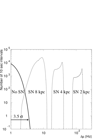
Figure 9: Background distribution and expected SN signal of $\Delta\mu$ for supernovae at different distances, in kpc. The smearing of the signal due to the fixed 10 sec observation window is taken into account (see Fig.6). Notice the logarithmic scale in $\Delta\mu$.

Fig.9 shows the distribution of the $\Delta\mu$ signal expectation for supernovae of type SN1987-A located at different distances, including the effect of the fixed 10 sec time-window location. The expected distribution in the absence of a supernova is also shown, for comparison.

The resulting $\Delta\mu$ distribution for the combined 1997 and 1998 data-sets can be seen in Fig.10, where a total live-time of 215 days has been accumulated. A cut on $\chi^{2}/\mathrm{n.d.f.}<1.3$ has been applied (leaving 99.9$\%$ of events), removing fake events which could still be seen in Fig.8. Without the $\chi^{2}/\mathrm{n.d.f.}$ cut, but cutting on $\mbox{ $\Delta\mu$}>4.0$ Hz, we have 1.7 background events per week. The spread of the background $\sigma_{\Delta\mu}^{\mathrm{noise}}=0.8$ Hz is the same for both years. This reflects the fact that the eleven additional OMs used in the 1998 set have high noise levels, and their spreads contribute little to reducing the total spread in Eq.10.

Figure 10: Distribution of $\Delta\mu$ after application of cuts, for 215 days of live-time. The vertical line is set at the level where we get a rate of one background event per year. 90$\%$ of supernova neutrino bursts located at 9.8 kpc distance would be seen above that cut.

Considering the background distribution of Fig.10, a SN signal detected with $90\%$ efficiency at a distance of 8, 4 and 2 kpc would correspond to an excess of 7, 29 and 116 standard deviations (see Fig.9). The line on Fig.10 indicates the $\Delta\mu$-level ($=4$ Hz) above which we would expect one fake event per year. Since the distribution in the figure is well fitted with a Gaussian, this number is found by fitting the data and integrating from that point and up to infinity. A cut on $\Delta\mu\geq 4$ Hz corresponds to a $90\%$ efficiency for a SN 1987A-like supernova located at a distance of 9.8 kpc.

6 Supernova sensitivity

The results of the analysis, along with numerical simulations, can be used to further assess the performance of Amanda as a supernova-burst detector.

Since the fitted noise-rate excess per OM is centered at zero in the absence of any supernova and has a known Gaussian spread, the number of dark noise background events is easily calculated for a given cut on $\Delta\mu$.

The signal that we expect to see is characterized by a frequency and a magnitude, both of which must be estimated to decide how to compute our signal-to-noise. The more elaborate estimates of the frequency of gravitational collapses are made using various methods and combining them [23]. We will limit ourselves to the most conservative guess of 1 supernova/century given in [32], since the performance of the detector does not depend strongly on that number, as will be shown.

The size of the signal depends on the distribution of progenitor stars in the Galaxy [22] and on the supernova neutrino-luminosity. The fraction of stars which could undergo a gravitational collapse is shown in Fig.1. We decided to use the measured luminosity of SN 1987A as an estimate of the signal-strength, since it is so far the only observation of an actual event.

Figure 11: Expected $\Delta\mu$ distributions at (full curve) and within (dotted curve) a distance of 10 kpc, shown in log-log scale. The dominant contribution to the signal is given by the closest stars, which appear in the tail of the distributions at high $\Delta\mu$ values. The vertical lines mark the $90\%$ detection efficiency lower limit.

Simulation studies were made in order to estimate the signal, for which we used the time-profile described in section 2. The effect of the 10 sec time-window inefficiency (see Sec.4) , as well as the Gaussian smearing due to dark-noise fluctuations, was then applied to a signal of strength given by Eq. 1. As an example, the resulting $\Delta\mu$-distribution for a supernova occurring at a distance of 10 kpc can be seen in Fig.11(full curve). If we fold in the probability distribution shown in Fig.1, we can also obtain the signal distribution for supernovae occurring within, rather then at a radius of 10 kpc from the Earth (see Fig.11, dotted curve).

With these definitions of background and signal (i.e. everything within a sphere of a given radius), it is now possible to define a performance parameter which we call signal-to-noise $S/N$ at a given distance. For this purpose, the $\Delta\mu$-distribution of progenitor stars within that distance is computed as well as the lower cut which keeps $90\%$ of stars above it. The signal $S$ above the $\Delta\mu$-cut is calculated, taking all efficiencies into account, as well as the estimated rate. Finally, the noise $N$ from the dark noise background for the same period of time and same cut on $\Delta\mu$ is readily computed from the Gaussian assumptions. Fig.12 shows the resulting $S/N$ parameter as a function of distance from the Earth. At a characteristic radius, a drastic drop in $S/N$ from very large values down to essentially zero occurs, which characterizes the detector performance.

Figure 12: The $S/N$-ratio as a function of distance for strings 1-10 ($S/N>1$ within 11 kpc, i.e. 60% of the Galaxy). $S/N=1$ corresponds to a cut at $\Delta\mu=5.5$ Hz. Inset: the same curve seen in a logarithmic scale.

We will therefore take the point at which $S/N=1$ as a natural measure of the performance of different detector configurations. Note that the distance that corresponds to that point does not depend strongly on the chosen $S/N$ value, due to the sharpness of the drop. For instance, a larger estimate for the gravitational collapse rate would not change that characteristic distance significantly. Indeed, using the different estimates found in the literature, of 1 SN every 100 [32], 47 [23] and 11 [33] years, the $S/N=1$ point would be located at 11 ($\sim 60\%$ Galaxy coverage), 11.3($63\%$) and 11.8($66\%$) kpc, respectively. The small differences are due to the steepness of the curve (see Fig.12). Amanda B10 is thus able to detect supernovae within a distance of 11 kpc with a S/N $>1$, i.e. to cover $\sim 60\%$ of the stars in the Milky Way with one background fake per century. The coverage for detector configurations with other $\sigma_{\Delta\mu}^{\mathrm{noise}}$-values is shown in Fig.13.

Figure 13: Percentage of the Galaxy coverage versus $\sigma_{\Delta\mu}^{\mathrm{noise}}$. Note that no specific detector setup is assumed in this figure.

If one lowers the requirement to accepting one background event per year and a supernova detection probability of $90\%$, the Galactic coverage is $70\%$. Even though the additional OMs in strings 5-10 have worse noise characteristics, they provide a significant improvement. Observe however, that this is mainly due to the very steep behavior of the distribution in Fig.1 in the range of 7-14 kpc around the bulge, where the star density is the highest.

The non-observation of any supernova signal can be used to put an upper limit on the rate of gravitational stellar collapses:

$$R_{\mathrm{c.l.}}=\frac{n_{\mathrm{c.l.}}}{\eta\epsilon\times T}$$ (11)

where $n_{\mathrm{c.l.}}$ is the upper bound at the 90$\%$ c.l. on the expected number of events, $\eta$ is the Galactic coverage (70$\%$), $\epsilon$ is the detection efficiency ($90\%$) and $T$ is the live time (215 days). Using the procedure described in [34] (with no candidates observed and one estimated background fake per year), we obtain an upper limit on the rate of gravitational stellar collapses at the $90\%$ c.l., of 4.3 events per year.

7 Amanda Supernova Trigger Algorithm (Asta)

The goal of the trigger is to detect a supernova event in real time, in order to send out a prompt alarm to the astronomical community, ahead of its optical observation. A future implementation of Asta  at the South Pole will make it possible to join SNEWS [35], a supernova early warning network of neutrino detectors. A first version of Asta  based on 11 days of data was presented in [36].

The online algorithm must be able to suppress background events which could fake a SN neutrino burst, especially those due to non-Gaussian variations of the noise rates. We must use a moving average which uses exclusively events occurring to the left, i.e. before the considered time-bin. We will refer to it as $MA_{\mathrm{left}}$, as opposed to $MA_{\mathrm{sym}}$, with the difference that the sum in Eq.5 is now taken from $(i-\mbox{$n_{\mathrm{window}}$})$ to $i$. In order to accommodate for faster variations of the data, we define an additional variable, the derivative of $MA_{\mathrm{left}}$ for each event $(i)$:

$$DER(i)=$$

$$[MA_{\mathrm{left}}(i)-MA_{\mathrm{left}}(i-1)]/{\Delta t}$$

where $\Delta t=100$ sec. It has been tested with numerical simulations that during normal data-taking conditions, the occurrence of a SN signal should not increase $DER(i)$ significantly.

Using the same OM selection as in the offline-analysis was found to be unsuitable for Asta, rejecting a large percentage of the events after applying a cut on $\chi^{2}/\mathrm{n.d.f.}<1.3$. Instead, we removed 117 known unstable OMs and then applied the cleaning algorithm described in section 4 on the 1998 data sample. This resulted in a set of 170 OMs that were then used to test the cuts on both the 1997 and 1998 data.

Figure 14: Tail of the background distribution after different cut levels: (dotted line) ’no cuts’, (dashed line) ’$\chi^{2}+DER$ cut’, (solid line) ’all cuts’. The vertical line indicates the $\Delta\mu$-cut that leaves one statistical fake per year. The live time is 296 days.

Fast time variations of the data ($S_{\mathrm{tot}}$) are not always corrected fully by moving-average subtraction. Taking this into account we decided to iterate, i.e. apply the moving-average correction a second time, on $RES$:

$$RES_{\mathrm{iter}}(RES(i))=$$ (13)

$$\hskip 14.22636ptRES(i)-MA_{\mathrm{left}}(RES(i))$$

A new $\Delta\mu$ can be calculated, as well as new variables $\chi^{2}_{\mathrm{iter}}$ and $DER_{\mathrm{iter}}$. The final cuts applied are: $\Delta\mu>4.1$ Hz, $|DER|<1\,\mathrm{s^{-2}}$, $\chi^{2}/\mathrm{n.d.f.}<1.3$, $|DER_{\mathrm{iter}}|<1\,\mathrm{s^{-2}}$ and $\chi^{2}_{\mathrm{iter}}/\mathrm{n.d.f.}<1.3$, leaving five triggers only, i.e. one every two months (see Fig.14). Note that these requirements leave the efficiency to trigger on a SN during stable data-taking conditions unaffected. In order to estimate the performance of the cuts as previously, we use $\sigma_{\Delta\mu}^{\mathrm{noise}}=0.85$ Hz and the cut $\Delta\mu>4.1$ Hz, resulting in a $65\%$ coverage of the Galaxy with $90\%$ detection efficiency. On top of the five fakes found experimentally, we expect statistically one background event per year. We note that all fakes have low significance and that already a cut on $\Delta\mu>5$ Hz can get rid of them, which would lower the Galactic coverage to $55\%$.

8 Discussion

The good overall performance of the detector is mainly due to the low noise of the OMs in strings 1-4. However, even if all OMs would be of the same type as those, 800 of them would still be required to cover $100\%$ of the Milky Way. From Eq.10 and Fig.13, it is clear that $\sigma_{\Delta\mu}^{\mathrm{noise}}$ is a crucial parameter for the detector performance and must be kept as small as possible.

Assuming a uniform detector with only one type of OMs, Eq.10 becomes:

$$\sigma_{\Delta_{\mu}}^{\mathrm{noise}}=\frac{\sigma_{\mathrm{OM}}}{\epsilon\sqrt{N_{\mathrm{OM}}}}$$ (14)

One sees from Eq.14 that increasing $N_{\mathrm{OM}}$ is a less efficient way of reducing $\sigma_{\Delta\mu}^{\mathrm{noise}}$ than increasing the collection efficiency $\epsilon$ or reducing $\sigma_{\mathrm{OM}}$, the spread in the dark-noise rate of each OM. Several technical improvements to the OMs can be considered, which affect $\sigma_{\mathrm{OM}}$, $\epsilon$ and $\sigma_{\Delta\mu}^{\mathrm{noise}}$:

• coating the OMs with wavelength-shifters would increase the photon-collection efficiency without affecting the noise rates.

• using PMTs with a larger cathode area would increase the efficiency, even though the noise level would go up.

• reducing the potassium levels in the pressure glass would reduce the dark noise spread.

• Fig.3 shows that there are ice-depths with larger transparency which are most suitable for SN detection. In fact, the transparency is expected to be extremely good at shallower depths [37, 38]. However, the muon flux is larger closer to the ice surface, producing more background Cherenkov light.

All these improvements have been investigated and we estimate that they can reduce the value of $\sigma_{\Delta\mu}^{\mathrm{noise}}$ by $20-40\%$ each.

Detailed investigations on after-pulsing in the range up to 1 msec are currently being pursued in order to optimize the choice of artificial dead-time. The effects of raising the PMT thresholds remain to be investigated. Finally, it may be noted that a sliding time-window, fitted to the supernova time-profile, rather than applied at arbitrary times, would increase the galactic coverage of the detector studied in this paper by an estimated $11\%$. One could even optimize the size of the window to fit the peaked part of the profile so that the ratio $\epsilon/\sigma_{\mathrm{OM}}$ is maximized. An additional $10\%$ could be gained in this way, even though it is clear that such optimization is partly model-dependent (for the model used here, a 4 sec time window would be optimal).

An uncertainty in the strength of the signal is the ${\bar{\nu}}_{e}$ temperature. In this paper, we use the same assumption as in [11] ($T_{\mbox{${\bar{\nu}}_{e}$}}=4$ MeV), but there is no precise prediction for this value and it may be lower (see e.g. [39]). Furthermore, corrections to inverse beta-decay cross-sections due to recoil and weak magnetism [40] would lower the resulting positron energy somewhat. On the other hand, this can be compensated in some measure by the performance of the present detector (680 OMs), which is expected to be higher than the configuration studied in this paper. With the planned transition to a detector of kilometer-cubed size, using thousands of OMs, full coverage of the Galaxy will be attained.

One of the greatest assets of Amanda with its low background rate is that it has the potential to see a supernova independently from other detectors. In the event of a discovery, the time profile and intensity of the burst could be studied. These aspects will be investigated in the future. Should an event occur in our Galaxy, the information that could presently be provided to the rest of the supernova community, is an estimate of $\Delta\mu$ and a time stamp associated with the event.

9 Conclusions

Amanda primarily aims at detecting high-energy neutrinos. However, by monitoring bursts of low-energy neutrinos, it is operating as a gravitational collapse detector as well. In the course of this analysis, a method has been developed and applied to filter the data and remove unstable periods and OMs. from disturbances. Furthermore, the $\chi^{2}$-based analysis method used here takes into account the varying statistical properties of different OMs. The sets of data taken in 1997 and 1998, corresponding to 215 days of live-time after cleaning, have been fully searched for supernova bursts occurring in our galaxy. No significant candidates were found. A conservative model of the supernovae-distribution in space and time has been used to assess the performance of the detector, resulting in an estimated coverage of the galaxy of $70\%$ with $90\%$ efficiency, with one expected background fake per year. This performance is satisfying, the more so since the primary design of Amanda is for high-energy neutrino detection. A real-time supernova detection algorithm, has been developed and tested on the 296 days of live time available. The algorithm turned out to be sufficiently robust and resulted in five fakes with the set of cuts chosen. We find that 800 OMs of the same type as those used in the first four strings of the array would suffice to cover the entire galaxy. It is also shown that this number can be reduced significantly, either by reducing the spread of the dark noise, or by improving the collection sensitivity of the OMs.

References

- [1] R. M. Bionta et al., Phys. Rev. Lett. 58 (1987) 1494–1496.
- [2] K. Hirata, et al., Phys. Rev. Lett. 58 (1987) 1490–1493.
- [3] K. Hirata, et al., Phys. Rev. D 38 (1988) 448–458.
- [4] K. Scholberg, in: 19th International Conference on Neutrino Physics and Astrophysics, 2000, hep-ex/0008044.
- [5] E. Alexeyev, et al., Nucl. Phys. B Suppl. 35 (1994) 270–272.
- [6] E. Andres, et al., Astropart. Phys. 13 (2000) 1–20.
- [7] V. A. Balkanov, et al., Phys. Atom. Nucl. 63 (2000) 951.
- [8] C. Carloganu, Nucl. Phys. Proc. Suppl. 85 (2000) 146–152.
- [9] S. Bottai, et al., Nucl. Phys. Proc. Suppl. 85 (2000) 153–156.
- [10] T. Montaruli, et al., Proceedings of the 26th International Cosmic Ray Conference (ICRC 99), Salt Lake City, UT HE.6.3.06.
- [11] F. Halzen, J. E. Jacobsen, E. Zas, Phys. Rev. D 49 (1994) 1758–1761.
- [12] C. Pryor, C. Roos, M. Webster, Astrophys. J. 329 (1988) 335–338.
- [13] R. Wischnewski, et al., in: Proceedings of the 24th International Cosmic Ray Conference, Rome, Vol. 1, Italy, 1995, pp. 658–661.
- [14] A.Biron, et al., Proposal submitted to the Physics Research Committee, DESY, PRC 97/05 (1997).
- [15] R. Wischnewski et al., Proceedings of the 26th International Cosmic Ray Conference (ICRC 99), Salt Lake City, UT HE.4.2.07.
- [16] R. C. Kennicutt, Astrophys. J. 277 (1984) 361.
- [17] A. Burrows, D. Klein, R. Gandhi, Phys. Rev. D 45 (1992) 3361–3385.
- [18] G. Raffelt, Stars as laboratories for fundamental physics, The University of Chicago Press, 1996.
- [19] J. F. Beacom, P. Vogel, Phys. Rev. D 58 (1998) 053010.
- [20] J. F. Beacom, P. Vogel, Phys. Rev. D 60 (1999) 033007.
- [21] J. N. Bahcall, R. M. Soneira, Astrophys. J. 44 (1980) 73.
- [22] J. N. Bahcall, T. Piran, Astrophys. J. 267 (1983) L77.
- [23] G. A. Tammann, W. Löffler, A. Schröder, Astrophys. J. Suppl. 92 (1994) 487–493.
- [24] Y. Fukuda, in First International Workshop on the Supernova Early Alert Network, Boston University, unpublished, 1998.
- [25] The LVD Collaboration, in: Proceedings of the 26th International Cosmic Ray Conference (ICRC 99), Salt Lake City, UT, 1999, HE.4.2.08.
- [26] F. Halzen, T. Stanev, E. Zas, Phys. Rev. D 45 (1992) 362–376.
- [27] F. Halzen, J. E. Jacobsen, E. Zas, Phys. Rev. D 53 (1996) 7359.
- [28] J. E. Jacobsen, Ph.D. thesis, University of Wisconsin, Madison (1996).
- [29] K. Woschnagg et al., Proceedings of the 26th International Cosmic Ray Conference (ICRC 99), Salt Lake City, UT HE.4.1.15.
- [30] B. E. A. Saleh, J. T. Tavolacci, M. C. Teich, IEEE J. Quant. Electron. QE-17 (1981) 2341–2350.
- [31] P. J. Brockwell, R. A. Davis, Introduction to Time Series and Forecasting, Springer Verlag, 1996.
- [32] A. Suzuki, Supernova Neutrinos, in Physics and Astrophysics of Neutrinos, Springer Verlag, 1994.
- [33] J. N. Bahcall, Neutrino Astrophysics, Cambridge University Press, 1989.
- [34] G. Feldman, R. Cousins, Phys. Rev. D 57 (1998) 3873–3889.
- [35] K. Scholberg, in: Proceedings of the 3rd Amaldi Conference on Gravitational Waves, 1999, astro-ph/9911359.
- [36] A. Silvestri, Diploma thesis: DESY-THESIS-2000-028, Zeuthen, ISSN 1435-8085 (2000).
- [37] P.Askebjer, et al., Science 267 (1995) 1147.
- [38] S.Tilav, et al., in: Proceedings of the 24th International Cosmic Ray Conference, Rome, Vol. 1, 1995, p. 1011.
- [39] B. Jegerlehner, F. Neubig, G. Raffelt, Phys. Rev. D 54 (1996) 1194–1203.
- [40] P. Vogel, J. Beacom, Phys. Rev. D 60 (1999) 053003.