Stellar radio astrophysics

Abstract

Radio emission has been detected from all the stages of stellar evolution across the HR Diagram. Its presence reveals both astrophysical phenomena and stellar activity which, otherwise, would not be detectable by other means. The development of large, sensitive interferometers has allowed us to resolve the radio structure of several stellar systems, providing insights into the mass transfer process in close binary systems. I review the main characteristics of the radio emission from several kinds of stars, paying special attention to those cases where such an emission originates in relativistic jets.

1 Introduction

If the stellar radio emission was restricted to solar-like activity levels, our knowledge of the Galaxy in radio wavelenghts would be significantly lesser. The radio flux density $S_{\nu}$ at a frequency $\nu$ of a star, measured at the earth, can be expressed in terms of the Rayleigh-Jeans approximation to the black body formula

$$S_{\nu}={2k\nu^{2}T_{\rm B}\Omega_{\rm S}\over c^{2}},$$ (1)

where $k$ is the Boltzmann’s constant, $T_{\rm B}$ is the brightness temperature and $\Omega_{\rm S}$ is the solid angle subtended by the star. The maximum distance at which a star like the Sun would be observable at 5 GHz with a radio telescope, assuming a typical minimum flux density of 1 mJy, is 0.2 pc for the quiet Sun, 0.3 pc for the slowly varying component, and 7.6 pc for the very strong solar radio bursts. If we take into account that the nearest star, Proxima Centauri, is 1.3 pc away, the solar-like emission would be observed only from a few nearby stars. In fact, the first radio stars detected were not really stars emitting at radio wavelengths but strong extragalactic sources.

Fortunately, the situation is much better. Since $S_{\nu}\propto T_{\rm B}\Omega_{\rm S}$, it is possible to detect radio stars that have either unusually large emitting surfaces, generally associated to stars having massive stellar winds, or enhanced brightness temperatures, associated to stars exhibiting powerful non-thermal radio emission.

Early efforts to observe radio stars concentrated on the nearby red supergiants. Kellermann & Pauliny-Toth ([1966]) reported a signal of 0.11$\pm$0.03 Jy while observing Betelgeuse at 2.8 cm, although no signal was detected on the next 11 nights. Seaquist ([1967]) reported the detection of Betelgeuse, with a flux density of 0.023$\pm$0.006 Jy at 2.8 cm, and $\pi$Aurigae, with a flux density of 0.031$\pm$0.009 Jy. However, none of these stars has been detected at such flux levels since then. The results obtained in these pioneering observations could have been affected by different factors, such as unknown problems with the equipment, the intrinsic variability of most radio stars, and confusion with background sources.

The fact that most of the solar radio emission occurs in a large variety of flares of varying lifetimes inspired the study of radio emission from non-solar type stars. Red dwarf stars were known to exhibit flares at optical wavelengths, and became obvious candidates for radio flare searches. In 1969 Bernard Lovell, at Jodrell Bank, pioneered these observations. The first indisputable observations of radio flare star emission were the detections of a radio flare in YZ CMi and in UV Ceti at 408 MHz, obtained using long baseline interferometers (Davis et al. [1978]). The construction of large aperture synthesis arrays in the mid 1970s allowed to perform reliable measurements of radio emission and marked the beginning of the stellar radio astronomy.

The advent of radio interferometry prompted a significant advance in the knowledge of radio stars. Thanks to this technique it was possible to obtain a) accurate positions, which allow to see if the position of a radio source coincides with that of a star, b) higher sensitivity, because all the data collected for long observing times can be added together, and c) a better determination of the variability, since a time-variable event is most certain if independent subsets of an array are detecting the same time-variable event. Since then, the field of stellar radio astronomy has advanced explosively. We are now able to image radio emission from stellar sources with unprecedented resolution and sensitivity. Thanks to these observational advances, the number and classes of stars known to be sources of radio emission have increased dramatically. As we will see, radio emission has been detected from all the stages of stellar evolution, from birth to death, and has revealed astrophysical phenomena and stellar activity that are not detectable by other means.

To illustrate the progress made in the field of stellar radio astrophysics, it is worth noting that two dedicated conferences were conducted in the past two decades. In 1984, a workshop on stellar continuum radio astronomy was held in Boulder (Hjellming & Gibson [1985]). That workshop reviewed the observational and theoretical work on radio stars from the first decade of the interferometer era. In 1995, a workshop was held in Barcelona, providing an overview of the rich and powerful sets of new radio observations accumulated over the past decade and new theoretical ideas and models arising from them (Taylor & Paredes [1996]).

2 Types of radio stars

The catalogue of Wendker ([1995]) of radio continuum emission from stars contains 3021 systems: 821 were detected at least once, and 2192 have only upper limits. A first look at this catalogue evidences both the variability and the low level of radio emission from the stars. The Hertzprung-Russell diagram for a subset of stellar detections is shown in Figure 1. The radio luminosity is indicated by the size of each circle. Radio emission has been detected from all the stages of stellar evolution across the HR diagram. The evolutionary state of a star in the diagram is closely related to its radio activity. Most of the main sequence and sub-giant objects are non-thermal emitters. In contrast, most of the giants and many O-B stars are thermal emitters, but they can be detected because of their large sizes. Novae and X-ray binaries are not shown since the active source is related to accretion onto a white dwarf and a neutron star or black hole, respectively, and not directly to their evolutionary state.

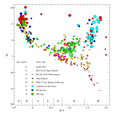
Figure 1: HR diagram showing the distribution of several types of stars (from Güdel [2002]).

The radio stars can be classified according to the underlaying cause of their enhanced radio luminosity (see also Seaquist [1993]). We can distinguish the following classes:

2.1 Stars undergoing mass loss

OB and Wolf-Rayet stars: These stars produce free-free (FF) emission associated to an optically thick wind. Non-thermal emission is also observed, due either to relativistic electrons embedded in the wind produced by Fermi acceleration in shock fronts or to collision between the winds of the two components of a binary.

Be stars: The FF emission is produced as a consequence of mass loss through an equatorial disk by centrifugal effects caused by the rapid rotation of the star.

Single red giants and supergiants: The winds of these evolved stars are cool and only partially ionized. They are detectable if the star is relatively nearby.

VV Cephei stars: Binaries containing a cool supergiant and a main sequence B companion. The FF emission comes from a subregion of the supergiant wind ionized by UV photons from the hotter companion.

Pre-main sequence stars: T Tauri stars that can be subdivided into two classes: classical T Tauri stars (CTT), which emit FF emission from ionized gas, and weak-lined T Tauri stars (WTT), which emit non-thermal radio emission from magnetically active regions.

2.2 Stars exhibiting enhanced solar activity

The sun exhibits non-thermal emission and flare activity associated with high-energy particles in the chromosphere and corona. The same phenomenon on larger scales is characteristic of many cool (primarily K-M) stars on and above the main sequence. The energy supply is thought to be the release of stellar magnetic field energy by reconnection of field lines. The magnetic fields may be generated by a dynamo mechanism.

Flare stars: Single stars that exhibit intense flares from X-rays to radio waves. The coronal gas is bound by magnetic loops of several 1000 G covering most of the stellar surface. The stellar flares are due to coherent emission (at lower frequencies) and incoherent gyrosynchrotron emission (at higher frequencies). Prototype stars are UV Ceti, YZ CMi and AD Leo.

Close binaries: The typical components of the RS Canis Venaticorum (RS CVn) binary systems are a solar-type star and a more evolved, cool subgiant. Their radio emission is generally accounted for by a gyrosynchrotron emission mechanism. The magnetic activity is enhanced by the high rotation rate of the active subgiant, which is synchronised to the period of orbital revolution by tidal coupling. Particle acceleration may also occur in the intrabinary plasma if the interaction between the fields of the two stars produce reconnection. These mechanisms may also occur in semi-detached systems (Algol binaries) and in contact binaries (W Ursae Majoris stars). The radio properties of Algols are similar to those of RS CVn systems, while W UMa stars are less luminous. The characteristics of the RS CVn systems are discussed in more detail in Section 4.

Pre-main sequence stars: Some of the properties of WTT stars are similar to those of RS CVn stars. The mechanism for producing the radio emission is gyrosynchrotron emission from starspot regions.

2.3 Chemically peculiar stars

CP stars or Bp-Ap stars: Main sequence stars characterized by over and under abundances of certain chemical elements and by strong (1-10 kG) dipolar magnetic fields. There are no convection motions in their stellar envelopes, and the magnetic field is thought to be a fossil remnant of the dynamo fields generated in the pre main-sequence phase. Their radio properties (flat radio spectrum, circular polarization, non-thermal $T_{\rm B}$) are consistent with gyrosynchrotron emission.

2.4 Radio emission related to mass transfer in binaries

The transfer process may involve Roche lobe overflow or stellar wind accretion from a normal star to a white dwarf (WD), neutron star (NS) or black hole (BH).

Cataclysmic variables: Classical novae are semi-detached binaries containing a main-sequence star and a WD. Nova outbursts (intervals of $\sim$10⁴ yr) occur when the accreted H-rich material accumulates on the outer surface of the WD and leads to a thermal runaway and explosive ejection of the outer envelope. FF emission comes from the expanding ionized ejecta. It is observed synchrotron radiation from particles accelerated in a shock (within the ejecta or in the interaction between the nova ejecta and a dense gas cloud). The magnetic cataclysmic variables (DQ Her and AM Her systems) contain a late-type MS and a magnetic WD, and the mass transfer process is modified by the presence of strong magnetic fields of 10⁵–10⁷ G. It has been observed highly variable flare-like non-thermal radio emission. Symbiotic stars are interacting binaries containing a cool (red) giant and a hot companion. These systems emit FF emission from a circumstellar ionized envelope.

X-ray binaries: The X-ray emission is produced by accretion of matter onto a compact companion. See more details in Section 5.

3 Linking the radio and optical reference frames

The determination of a suitable celestial reference frame is of fundamental importance in astronomy, in particular when dealing with the highly increasing accuracy of the observations. The International Celestial Reference System (ICRS) is a quasi-inertial reference system based upon the positions of a number of extragalactic objects. The International Celestial Reference Frame (ICRF) is the radio realization of the ICRS, and it is defined by the positions of 212 extragalactic radio sources derived from VLBI observations (Ma et al. [1998]). The ICRF is the most precise reference system ever materialized. On the other hand, the Hipparcos astrometry space mission has observed $\sim$120 000 objects evenly distributed over the sky, providing astrometric parameters with a precision of $\sim$1 mas and $\sim$1 mas yr^-1. The positions and proper motions of the Hipparcos Catalogue define an optical reference frame that represents a materialization of the ICRS at optical wavelenghts.

Thus, to determine the best celestial reference frame for astronomical purposes, it becomes necessary to link the Hipparcos Reference Frame to the ICRF through objects whose positions and/or proper motions can be referred to both systems. The observation of radio stars is one of the methods used for this link. For these observations, it is important to select targets with small angular diameters (non-thermal emitters) and bright enough in the radio band to provide accurate positions. Multiple-epoch phase referenced VLBI observations of selected radio stars (active non-thermal radio emitters which are also optically bright) have been conducted as part of an on-going astrometric program to link the Hipparcos reference frame to the extragalactic reference frame (Lestrade et al. [1999]). The observational campaigns performed for this link prompted a significant advance in the study of radio stars. The preferred radio sources for these observations were RS CVn binaries and X-ray binaries. These systems will be discussed in detail in the following sections.

4 RS CVn binaries

RS CVn are one of the most common kind of radio detected stars. RS CVn systems are close, chromospherically active binary systems whose enhanced emission can be detected over a wide range of the spectral domain, from the X-ray to the radio region. Most of the phenomena observed in these systems at different wavelengths are attributed to the presence of magnetic fields generated by a dynamo mechanism.

In general, the radio emission from RS CVn binary systems is quite variable, with luminosity levels in the range 10¹⁴$-$10¹⁹ erg s^-1 Hz^-1 at centimeter wavelengths (Morris & Mutel [1988]; Drake et al. [1992]). Typical features of the radio emission from these systems are: a) low-level (quiescent) emission with moderately circularly polarized emission (degree of circular polarization $\pi_{\rm c}\leq$30–40%) and flat or negative spectrum (spectral index $\alpha\leq 0$, where $S_{\nu}\propto\nu^{\alpha}$); or b) high-level (flaring) emission, unpolarized or weakly polarized ($\pi_{\rm c}\leq 10$%), and with positive spectral index $\alpha$; or c) high-intensity, short-duration outbursts with high degrees of circular polarization (see Gunn [1996] for a review on RS CVn binary systems). The mechanisms generally invoked to account for the observed radio emission are gyrosynchrotron, synchrotron and coherent (electron-cyclotron maser or plasma radiation) processes. For reviews on these radio emission mechanisms see, for instance, Dulk ([1985]) and Güdel ([2002]).

Linear polarization is not expected to be present in the radio emission from RS CVn systems due to the large Faraday rotation in the stellar coronae. Circular polarization measurements are, thus, the main input for the understanding of the magnetic fields of these stars. Mutel et al. ([1987]) studied a small sample of late-type binaries, mainly of the RS CVn class, and found that non-eclipsing (low inclination angle) systems have an average circular polarization in their quiescent emission significantly larger than that for eclipsing systems. Multifrequency polarization observations (e.g., Mutel et al. [1987]; Umana et al. [1993]; White & Franciosini [1995]; García-Sánchez et al. [2003]) revealed properties of both low-level and high-level emission sources, showing a reversal in the sense of polarization between 1.4 GHz and 5 GHz for non-eclipsing systems. White & Franciosini ([1995]) proposed that weak, highly polarized, coherent plasma emission may be associated with the polarization inversion observed at low frequencies. In addition, White & Franciosini ([1995]) found an increase of the degree of polarization with increasing frequency at high frequencies, independently of the shape of the spectrum, contrary to what is expected according to gyrosynchrotron models.

The large coronal sizes of active RS CVn systems could be accounted for by the gradual release of magnetic free energy built up by the interaction of the stellar magnetic fields of the two components of the binary (Uchida & Sakurai [1983]). Differential rotation in the stars may produce a twisting of magnetic flux tubes, and the reconnection of loops can give rise to a extended corona between the two components. VLBA and VLA observations of the quiescent emission from UX Ari by Beasley & Güdel ([2000]) resolved the source on linear scales comparable to the projected separation of the components, which indicates the existence of large magnetic structures. They also detected circular polarization with a polarization gradient across the radio source, which suggests the existence of interacting magnetic fields between the components or a large magnetic loop anchored to one component.

The non-thermal nature of the electron distribution responsible for the flaring emission from RS CVn systems seems to be well established. The quiescent emission has been interpreted in two different ways, based on different assumptions for the distribution of the population of electrons responsible for the emission observed, namely gyrosynchrotron emission from a Maxwellian (thermal) distribution or from a power-law (non-thermal) distribution (Drake et al. [1992]; Chiuderi-Drago & Franciosini [1993]). However, a thermal gyrosynchrotron emission model with uniform magnetic field predicts a spectral index $\alpha=-8$ after the peak, whereas the spectra observed are much flatter. Thermal emission in a magnetic field $B$ decreasing as $B\propto r^{-1}$, where $r$ is the distance from the active star, may reproduce the observed quiescent spectrum, but the magnetic field structure seems unrealistic. Emission from a non-thermal distribution appears to be the most plausible explanation for the observed properties of the quiescent emission.

One of the most active sources at radio wavelengths is the system UX Ari. The radio emission of this system is highly variable. VLBI observations of UX Ari have shown that also the source structure is variable. During strong flares a compact bright source of stellar size and a fainter component of dimensions comparable to the binary separation are observed, as can be seen in the left image plotted in Figure 2, obtained by Mutel et al. (1985). At lower flux levels, however, only the extended component is present (Massi et al. [1988]). The $T_{\rm B}$, the sizes measured by VLBI and the moderate circular polarization are consistent with gyrosynchrotron radiation by electrons of a few MeV or less spiraling in fields of $\sim$10 to $\sim$100 G (Dulk [1985]). VLBI maps showing a clear variation of the source structure with time have been obtained by Franciosini et al. ([1999]). Another example of the core-halo morphology is the VLBI image of the binary system HR 5110 obtained by Ransom et al. ([2003]), in which the core source has a smaller size than that of the chromospherically active K subgiant component, whereas the halo size is almost twice as much as the separation of the centers of the K and F stars.

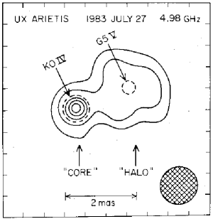
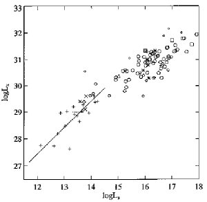
Figure 2: Left: VLBI map of the RS CVn system UX Ari. A core-halo structure is visible (from Mutel et al. [1985]). Right: Correlation between radio and X-ray luminosities of different types of active stars. The RS CVn binaries are marked as circles (from Güdel & Benz [1993]).

A correlation between quiescent radio (5–8 GHz) and X-ray luminosity of magnetically active stars has been found (see Figure 2, right), which suggests that radio and X-ray emissions are activity indicators that reflect the level of magnetic activity (Güdel & Benz [1993]). In particular, for RS CVn and Algol systems, the correlation between the radio and the X-ray luminosities is $L_{\rm R}\propto L_{\rm X}^{1.0-1.3}$. Assuming that the release of magnetic energy accumulated by the stretching of magnetic lines caused by turbulent motions is a heating mechanism of coronal loops, Chiuderi-Drago & Franciosini ([1993]) estimated that if this energy is radiated away in the form of X-rays, then $L_{\rm X}\propto B^{2}V$, where $B$ is the magnetic field and $V$ is the loop’s volume. On the other hand, these authors assumed a power-law electron population of index $\delta$ in the same loop emitting optically thin gyrosynchrotron emission, so the radio luminosity is $L_{\rm R}\propto B^{-0.22+0.96\delta}V$. From the above relationships it follows that $L_{\rm R}\propto L_{\rm X}^{0.45\delta-0.11}V^{1.11-0.45\delta}$. For $\delta=3$, neglecting the volume correction, they found $L_{\rm R}\propto L_{\rm X}^{1.24}$, in agreement with the empirical values.

The characteristics of the radio and X-ray emission from Algol systems are very similar to those of RS CVn binaries. In fact, some binaries like HR 5110 show typical features of both systems, and their classification as belonging to one class or the other is not simple. Unlike RS CVn binaries, the radio emission from Algol systems is usually unpolarized or very weakly polarized even during quiescence. A VLBA image of Algol by Mutel et al. ([1998]) represents the first evidence for double-lobed structure in the radio corona of an active late-type star in the quiescent state. The individual lobes are strongly circularly polarized and of opposite helicity, although the total emission is only weakly polarized. The radio emission is suggested to be gyrosynchrotron emission from optically thin emission regions containing mildly relativistic electrons in a dipolar magnetic field. Using VLBI astrometry, Lestrade et al. ([1993]) found that the radio emission from Algol is related to the magnetically active K subgiant component.

5 X-ray binaries

An X-ray binary is a binary system containing a compact object, either a neutron star or a stellar-mass black hole, that emits X-rays as a result of a process of accretion of matter from the companion star. Several scenarios have been proposed to explain this X-ray emission, depending on the nature of the compact object, its magnetic field in the case of a neutron star, and the geometry of the accretion flow. The accreted matter is accelerated to relativistic speeds, transforming its potential energy provided by the intense gravitational field of the compact object into kinetic energy. Assuming that this kinetic energy is finally radiated, the accretion luminosity can be computed, finding that this mechanism provides a very efficient source of energy, even much higher efficiency than that for nuclear reactions.

On its way to the compact object, the accreted matter carries angular momentum and usually forms an accretion disk around it. The matter in the disk looses angular momentum due to viscous dissipation, which produces a heating of the disk, and falls towards the compact object in a spiral trajectory. The black body temperature of the last stable orbit in the case of a BH accreting at the Eddington limit is given by:

$$T\sim 2\times 10^{7}M^{-1/4}$$ (2)

where $T$ is expressed in Kelvin and $M$ in $M_{\odot}$ (Rees 1984). For a compact object of a few solar masses, $T\sim 10^{7}$ K. At this temperature the energy is mainly radiated in the X-ray domain.

In High Mass X-ray Binaries (HMXBs) the donor star is an O or B early type star of mass in the range $\sim 8$–$20$ $M_{\odot}$ and typical orbital periods of several days. HMXBs are conventionally divided into two subgroups: systems containing a B star with emission lines (Be stars), and systems containing a supergiant (SG) O or B star. In the first case, the Be stars do not fill their Roche lobe, and accretion onto the compact object is produced via mass transfer through a decretion disk. Most of these systems are transient X-ray sources during periastron passage. In the second case, OB SG stars, the mass transfer is due to a strong stellar wind and/or to Roche lobe overflow. The X-ray emission is persistent, and large variability is usual. The most recent catalogue of HMXBs was compiled by Liu et al. ([2000]), and contains 130 sources.

In Low Mass X-ray Binaries (LMXBs) the donor has a spectral type later than B, and a mass $\leq 2$ $M_{\odot}$. Although typically is a non-degenerated star, there are some examples where the donor is a WD. The orbital periods are in the range 0.2–400 hours, with typical values $<24$ hours. The orbits are usually circular, and mass transfer is due to Roche lobe overflow. Most of LMXBs are transients, probably as a result of an instability in the accretion disk or a mass ejection episode from the companion. The typical ratio between X-ray to optical luminosity is in the range $L_{\rm X}/L_{\rm opt}\simeq 100$–$1000$, and the optical light is dominated by X-ray heating of the accretion disk and the companion star. Some LMXBs are classified as ‘Z’ and ‘Atoll’ sources, according to the pattern traced out in the X-ray color-color diagram. ‘Z’ sources are thought to be weak magnetic field neutron stars of the order of $10^{10}$ G with accretion rates around 0.5–1.0 $\dot{M}_{\rm Edd}$. ‘Atoll’ sources are believed to have even weaker magnetic fields of $\leq 10^{8}$ G and lower accretion rates of 0.01–0.1 $\dot{M}_{\rm Edd}$. The most recent catalogue of LMXBs was compiled by Liu et al. (2001), and contains 150 sources.

Recently, Grimm et al. ([2002]) estimated that the total number of X-ray binaries in the Galaxy brighter than 2$\times 10^{34}$ erg s^-1 is about 705, being distributed as $\sim$325 LMXBs and $\sim$380 HMXBs.

5.1 Radio emitting X-ray binaries (REXBs)

The first X-ray binary known to display radio emission was Sco X-1 in the late 1960s. Since then, many X-ray binaries have been detected at radio wavelengths with flux densities $\geq 0.1$–$1$ mJy. The flux densities detected are produced in small angular scales, which rules out a thermal emission mechanism. The most efficient known mechanism for production of intense radio emission from astronomical sources is the synchrotron emission mechanism, in which highly relativistic electrons interacting with magnetic fields produce intense radio emission that tends to be linearly polarized. The observed radio emission can be explained by assuming a spatial distribution of non-thermal relativistic electrons, usually with a power-law energy distribution, interacting with magnetic fields.

Since some REXBs, like SS 433, were found to display elongated or jet-like features, like in AGN and quasars, it was proposed that flows of relativistic electrons were ejected perpendicular to the accretion disk, and were responsible for synchrotron radio emission in the presence of a magnetic field. Models of adiabatically expanding synchrotron radiation-emitting conical jets may explain some of the characteristics of radio emission from X-ray binaries (Hjellming & Johnston [1988]). Several models have been proposed for the formation and collimation of the jets, including the presence of an accretion disk close to the compact object, a magnetic field in the accretion disk, or a high spin for the compact object. However, there is no clear agreement on what mechanism is exactly at work.

There are eight radio emitting HMXBs and 35 radio emitting LMXBs. Since the strong magnetic field of the X-ray pulsars disrupts the accretion disk at several thousand kilometers from the neutron star, there is no inner accretion disk to launch a jet and no synchrotron radio emission has ever been detected in any of these sources. Although the division of X-ray binaries in HMXBs and LMXBs is useful for the study of binary evolution, it is probably not important for the study of the radio emission in these systems, where the only important aspect seems to be the presence of an inner accretion disk capable of producing radio jets. However, the eight radio emitting HMXBs include six persistent and two transient sources, while among the 35 radio emitting LMXBs we find 11 persistent and 24 transient sources. The difference between the persistent and transient behavior clearly depends on the mass of the donor.

Excluding X-ray pulsars, $20$ to $25\%$ of the catalogued galactic X-ray binaries have been detected at radio wavelengths regardless of the nature of the donor. The corresponding ratio of detected/observed sources is probably much higher. However, it is difficult to give reliable numbers, since observational constrains arise when considering transient sources observed in the past (large X-ray error boxes, single dish and/or poor sensitivity radio observations, etc.), and likely many non-detections have not been published.

5.2 Microquasars

A microquasar is a radio emitting X-ray binary displaying relativistic radio jets. The name was given not only because of the observed morphological similarities between these sources and the distant quasars but also because of physical similarities, since when the compact object is a black hole, some parameters scale with the mass of the central object (Mirabel & Rodríguez [1999]). A schematic illustration comparing some parameters in quasars and microquasars is shown in Figure 3.

From Eq. 2, a typical temperature of a microquasar containing a stellar-mass black hole is $T\sim 10^{7}$ K, while that of a quasar containing a supermassive black hole ($10^{7}$–$10^{9}$ $M_{\odot}$) is $T\sim 10^{5}$ K. This explains why in microquasars the accretion luminosity is radiated in X-rays, while in quasars it is radiated in the optical/UV domain. The characteristic jet sizes seem to be proportional to the mass of the black hole. Radio jets in microquasars have typical sizes of a few light years, while in quasars may reach distances of up to several million light years. The timescales are also directly scaled with the mass of the black hole following $\tau\simeq R_{\rm S}/c=2GM_{\rm X}/c^{3}\propto M_{\rm X}$. Therefore, phenomena that take place in timescales of years in quasars can be studied in minutes in microquasars. Thus, microquasars mimic, on smaller scales, many of the phenomena seen in AGNs and quasars, but allow a better and faster progress in the understanding of the accretion/ejection processes that take place near compact objects.

The current number of microquasars is $\sim$16 among the 43 catalogued REXBs. Some authors (Fender 2001) have proposed that all REXBs are microquasars, and would be detected as such provided that there is enough sensitivity and/or resolution in the radio observations. The known microquasars, compiled from different sources, are listed in Table 1.

Table 1: Microquasars in our Galaxy

Name $\&$ Position	System	$D$	$P_{\rm orb}$	$M_{\rm compact}$	Activity	$\beta_{\rm apar}$	$\theta$(c)	Jet size
(J2000.0)	type(a)	(kpc)	(d)	$(M_{\odot})$	radio(b)			(AU)
High Mass X-ray Binaries (HMXB)
LS I +61 303	B0V	2.0	26.5	$-$	p	$\geq$0.4	$-$	10$-$700
$02^{\rm h}40^{\rm m}$31 ${\hbox to0.0pt{.\hss}}^{\rm s}$66	+NS?
$+61^{\circ}13^{\prime}$45${\hbox to0.0pt{.\hss}}^{\prime\prime}$6
V4641 Sgr	B9III	$\sim 10$	2.8	9.6	t	$\geq 9.5$	$-$	$-$
$18^{\rm h}19^{\rm m}$21${\hbox to0.0pt{.\hss}}^{\rm s}$48	+BH
$-25^{\circ}25^{\prime}$36${\hbox to0.0pt{.\hss}}^{\prime\prime}$0
LS 5039	O6.5V((f))	2.9	4.4	1$-$3	p	$\geq 0.15$	$<81^{\circ}$	10$-$1000
$18^{\rm h}26^{\rm m}$15${\hbox to0.0pt{.\hss}}^{\rm s}$05	+NS?
$-14^{\circ}50^{\prime}$54${\hbox to0.0pt{.\hss}}^{\prime\prime}$24
SS 433	evolved A?	4.8	13.1	11$\pm$5?	p	0.26	$79^{\circ}$	$\sim 10^{4}$$-$$10^{6}$
$19^{\rm h}11^{\rm m}$49${\hbox to0.0pt{.\hss}}^{\rm s}$6	+NS
$+04^{\circ}58^{\prime}58^{\prime\prime}$
Cygnus X-1	O9.7Iab	2.5	5.6	10.1	p	$-$	40∘	$\sim 40$
$19^{\rm h}58^{\rm m}$21${\hbox to0.0pt{.\hss}}^{\rm s}$68	+BH
$+35^{\circ}12^{\prime}$05${\hbox to0.0pt{.\hss}}^{\prime\prime}$8
Cygnus X-3	WNe	9	0.2	$-$	p	0.69	73∘	$\sim 10^{4}$
$20^{\rm h}32^{\rm m}$25${\hbox to0.0pt{.\hss}}^{\rm s}$78	+BH?
$+40^{\circ}57^{\prime}$28${\hbox to0.0pt{.\hss}}^{\prime\prime}$0
Low Mass X-ray Binaries (LMXB)
XTE J1118+480	K7V$-$M0V	1.9	0.17	6.9$\pm$0.9	t	$-$	$-$	$\leq 0.03$
$11^{\rm h}18^{\rm m}$10${\hbox to0.0pt{.\hss}}^{\rm s}$85	+BH
$+48^{\circ}02^{\prime}$12${\hbox to0.0pt{.\hss}}^{\prime\prime}$9
Circinus X-1	Subgiant	5.5	16.6	$-$	t	$\geq 0.1$	$>70^{\circ}$	$>10^{4}$
$15^{\rm h}20^{\rm m}$40${\hbox to0.0pt{.\hss}}^{\rm s}$9	+NS
$-57^{\circ}10^{\prime}01^{\prime\prime}$
XTE J1550$-$564	G8$-$K5V	5.3	1.5	9.4	t	$>2$	$-$	$\sim 10^{3}$
$15^{\rm h}50^{\rm m}$58${\hbox to0.0pt{.\hss}}^{\rm s}$70	+BH
$-56^{\circ}28^{\prime}$35${\hbox to0.0pt{.\hss}}^{\prime\prime}$2
Scorpius X-1	Subgiant	2.8	0.8	1.4	p	$0.68$	$44^{\circ}$	$\sim 40$
$16^{\rm h}19^{\rm m}$55${\hbox to0.0pt{.\hss}}^{\rm s}$1	+NS
$-15^{\circ}38^{\prime}25^{\prime\prime}$
GRO J1655$-$40	F5IV	3.2	2.6	7.02	t	1.1	$72^{\circ}$$-$$85^{\circ}$	8000
$16^{\rm h}54^{\rm m}$00${\hbox to0.0pt{.\hss}}^{\rm s}$25	+BH
$-39^{\circ}50^{\prime}$45${\hbox to0.0pt{.\hss}}^{\prime\prime}$0
GX 339$-$4	$-$	$\sim 4$	1.76	5.8$\pm$0.5	t	$-$	$-$	$<$ 4000
$17^{\rm h}02^{\rm m}$49${\hbox to0.0pt{.\hss}}^{\rm s}$5	+BH
$-48^{\circ}47^{\prime}23^{\prime\prime}$
1E 1740.7$-$2942	$-$	8.5?	12.5?	$-$	p	$-$	$-$	$\sim 10^{6}$
$17^{\rm h}43^{\rm m}54$${\hbox to0.0pt{.\hss}}^{\rm s}$83	+BH ?
$-29^{\circ}44^{\prime}$42${\hbox to0.0pt{.\hss}}^{\prime\prime}$60
XTE J1748$-$288	$-$	$\geq 8$	?	$>4.5$?	t	1.3	$-$	$>10^{4}$
$17^{\rm h}48^{\rm m}$05${\hbox to0.0pt{.\hss}}^{\rm s}$06	+BH?
$-28^{\circ}28^{\prime}$25${\hbox to0.0pt{.\hss}}^{\prime\prime}$8
GRS 1758$-$258	$-$	8.5?	18.5?	$-$	p	$-$	$-$	$\sim 10^{6}$
$18^{\rm h}01^{\rm m}$12${\hbox to0.0pt{.\hss}}^{\rm s}$40	+BH ?
$-25^{\circ}44^{\prime}$36${\hbox to0.0pt{.\hss}}^{\prime\prime}$1
GRS 1915+105	K$-$M III	12.5	33.5	14$\pm$4	t	1.2$-$1.7	$66^{\circ}$$-$$70^{\circ}$	$\sim 10$$-$$10^{4}$
$19^{\rm h}15^{\rm m}$11${\hbox to0.0pt{.\hss}}^{\rm s}$55	+BH
$+10^{\circ}56^{\prime}$44${\hbox to0.0pt{.\hss}}^{\prime\prime}$7

Notes: ^(a) NS: neutron star; BH: black hole. ^(b) p: persistent; t:transient. ^(c) jet inclination.

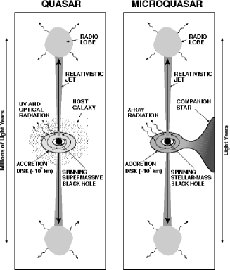
Figure 3: Comparative illustration of the analogy between quasars and microquasars. Note the extreme differences in the order of magnitude of the physical parameters involved (from Mirabel & Rodríguez [1998]).

5.2.1 Relativistic effects

The modern interferometers, working at radio wavelengths, are the only instruments that have provided a direct view of the most spectacular phenomena in microquasars. Their angular resolution well below the sub-arcsecond level allow us to follow the path and brightness decay of plasma clouds (plasmons) ejected along the relativistic jets into opposite directions. Due to the huge velocities involved, the effects predicted by the theory of Special Relativity must be taken into account for a correct interpretation of the observed data. Among them, we have the illusion of superluminal motion, as well as the difference in apparent brightness between the approaching and the receding jet due to relativistic aberration of light.

a) Apparent superluminal motion:

Let us assume that a source ejects two identical plasma clouds into opposite directions. The illusion of superluminal motion occurs for an ejection velocity $v=\beta c$ close to the speed of light and a rather small angle $\theta$ with respect to the line of sight. The fact that the approaching condensation reduces its distance to the observer by an amount $vt\cos{\theta}$ makes the light travel time towards the observer progressively shorter. The apparent velocity measured is thus given by:

$$v_{\rm a,r}={v\sin{\theta}\over(1\mp\beta\cos{\theta})},$$ (3)

for the approaching and the receding clouds, respectively. The minus sign, corresponding to the approaching case, may lead to a value of $v_{\rm a}$ arbitrarily large provided that $\beta$ and $\cos{\theta}$ approach unity. The first galactic object observed with superluminal motion was the microquasar GRS 1915+105 (Mirabel & Rodríguez [1994]). Until then, such relativistic illusion had been observed only in extragalactic objects like quasars. Figure 4 shows the time evolution of a GRS 1915+105 eruption in 1994, a bipolar ejection of two plasmons going away from the central core. Assuming a kinematical distance estimate to GRS 1915+105 of 12.5 kpc, the observed proper motions of the plasma clouds translate into apparent velocities of 1.25 and 0.65 times the speed of light. Other confirmed cases of superluminal sources in the Galaxy are the microquasars GRO J1655$-$40, XTE J1748$-$288, V4641 Sgr and XTE J1550$-$564.

Figure 4: VLA multiepoch observations at 3.6 cm wavelength of the superluminal ejection of GRS 1915+105 in 1994. The approaching component, to the left, appeared to move at $1.25c$ and be brighter than the receding one, to the right, which moved with an apparent velocity of $0.65c$ (from Mirabel & Rodríguez [1994]).

b) Relativistic aberration:

This effect is usually know as Doppler boosting. As above, let us assume that the two plasma clouds ejected into opposite directions are identical, with a radiation flux density $S_{0}$ in their respective reference frame. The synchrotron spectrum of each cloud, as a function of frequency $\nu$, follows a power-law $S_{0}\propto\nu^{\alpha}$, being $\alpha$ the so-called spectral index (usually $\alpha\simeq-0.7$). In the reference frame of the observer, the resulting flux density appears to be different from $S_{0}$. Let $S_{\rm a,r}$ be the flux density observed from the approaching and the receding clouds, respectively. The relationship between the emitted and observed flux density is given by:

$$S_{\rm a,r}={S_{0}\over\left[\Gamma(1\mp\beta\cos{\theta})\right]^{k-\alpha}},$$ (4)

where $\Gamma=1/\sqrt{1-\beta^{2}}$ is the bulk Lorentz factor, and the constant $k$ takes the values 3 or 2 depending on the case of discrete clouds or a continuous jet, respectively.

If $\theta$ is small ($\leq 10^{\circ}$) and $\beta$ close to unity, the brightness of the approaching cloud is considerably boosted and it may look thousands of times brighter than the receding one. This is the so-called Doppler favouritism, which only allows to see one side of the jet condensations in very distant quasars, where a strong amplification is needed for the emission to be detectable. This effect is shown in Figure 4, where the approaching jet seems to be faster and clearly brighter than the opposite counter-jet.

5.2.2 Accretion disk and jet ejection

The theoretical models attempting to understand the jet formation and its connection with the accretion disk had a seminal contribution in the works by Blandford & Payne ([1982]). These authors explored the possibility of extracting energy and angular momentum from the accretion disk by means of a magnetic field whose lines extend towards large distances from the disk surface. Their main result was the confirmation of the theoretical possibility to generate a flow of matter from the disk itself towards outside, provided that the angle between the disk and the lines was smaller than 60^∘. Later on, the flow of matter is collimated at large distances from the disk by the action of a toroidal component of the magnetic field. In this way, two opposite jets could be formed flowing away perpendicularly to the accretion disk plane.

To confirm observationally the link between accretion disk and the genesis of the jets is by no means an easy task. The collimated ejections in GRS 1915+105 provide one of the best studied cases supporting the proposed disk/jet connection. In Figure 5, from Mirabel et al. ([1998]), simultaneous observations are presented at radio, infrared and X-ray wavelengths. The data show the development of a radio outburst, with a peak flux density of about 50 mJy, as a result of a bipolar ejection of plasma clouds. However, previous to the radio outburst there was a clear precursor outburst in the infrared. The simplest interpretation is that both flaring episodes, radio and infrared, were due to synchrotron radiation generated by the same relativistic electrons of the ejected plasma. The adiabatic expansion of plasma clouds in the jets causes losses of energy of these electrons and, as a result, the spectral maximum of their synchrotron radiation is progressively shifted from the infrared to the radio domain.

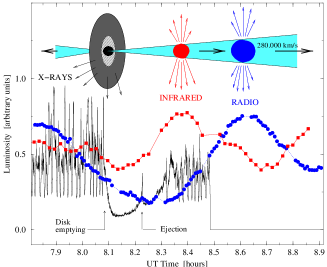
Figure 5: Multi-wavelength behaviour of the microquasar GRS 1915+105 as observed in September 8th 1997 (Mirabel et al. [1998]). The radio data at 3.6 cm (grey squares) were obtained with the VLA interferometer; the infrared observations at 2.2 micron (black squares) are from the UKIRT; the continuous line is the X-ray emission as observed by RXTE in the 2–50 keV range.

It is also important to note the behaviour of the X-ray emission in Figure 5. The emergence of jet plasma clouds, that produces the infrared and radio flares, seems to be accompanied by a sharp decay and hardening of the X-ray emission (8.08–8.23 h UT in the figure). The X-ray fading is interpreted as the disappearance, or emptying, of the inner regions of the accretion disk (Belloni et al. [1997]). Part of the matter content in the disk is then ejected into the jets, perpendicularly to the disk, while the rest is finally captured by the central black hole. Additionally, Mirabel et al. ([1998]) suggest that the initial time of the ejection coincides with the isolated X-ray spike just when the hardness index suddenly declines (8.23 h UT). The recovery of the X-ray emission level at this point is interpreted as the progressive refilling of the inner accretion disk with a new supply of matter until reaching the last stable orbit around the black hole.

This behaviour in the light curves of GRS 1915+105 has been repeatedly observed by different authors (e.g. Fender et al. [1997]; Eikenberry et al. [1998]), providing thus a solid proof of the so-called disk/jet symbiosis in accretion disks. All the observed events took less than half an hour to occur, and their equivalent in quasars, or AGNs, would require a much longer time span, a minimum of some few years. Despite the complexity in the GRS 1915+105 light curves, the episodes of X-ray emission decay with associated hardening are reminiscent of the well known low/hard state typical of persistent black hole candidates (Cygnus X-1, 1E 1740.7$-$2942, GRS 1758$-$258 and GX 339$-$4). The transitions towards this state are often accompanied by radio emission with flat spectrum, interpreted as due to the continuous creation of compact synchrotron jets partially self-absorbed.

It is worth mentioning the observational work by Marscher et al. ([2002]), who presented evidence of the disk/jet symbiosis also in an AGN, the active galaxy 3C 120. Using VLBI techniques they observed episodes of ejection of superluminal plasma just after the decay and hardening of the X-ray emission. This is precisely the same behaviour displayed by GRS 1915+105. The events in 3C 120 seem to be recurrent with an interval of one year, which is consistent with a mass of the compact object of $\sim 10^{7}$ $M_{\odot}$. Such observations strongly support the idea of continuity between galactic microquasars and AGNs in the Universe.

5.2.3 Precession

Historically, the first microquasar discovered was SS 433 (see Margon 1984). For many years it was considered a mere curiosity in the galactic fauna. Its plasma jets are ejected into the interstellar space at a speed of 0.26c, and precess with a period of 163 days. The flight of plasma clouds along the jets can be followed spectroscopically by means of their emission lines, whose redshift or blueshift agrees with a simple model of conical precession. SS 433 is the only microquasar where such lines have been detected so far, thus demonstrating the barionic nature of the ejecta at least in one case. The kinematic twin-jet model for SS 433 explains not only the radial velocity behaviour of the optical jets, but also the details of the proper motions of radio jets to scales of a few arc seconds (Figure 6) (Hjellming & Johnston [1981]; Stirling et al. [2002]). Other microquasars, such as LS I +61 303, V4641 Sgr, GRO J1655$-$40 and GRS 1915+105, might also be precessing systems, although this possibility needs further confirmation.

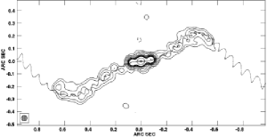
Figure 6: Left: 5 GHz image of SS 433 obtained with MERLIN. A kinematic model locus has been plotted (from Stirling et al. [2002]). Right: VLA image at 1465 MHz of the W50 nebula surrounding SS 433 at the center. Traces of the interaction of the jets of SS 433 with the surrounding gas are visible (from Dubner et al. [1998]).

5.2.4 Strong radio events

Cygnus X-3 has been the subject of intensive study during the last decades, specially after the discovery of its giant radio outbursts in 1972 (Gregory et al. [1972]). During strong outbursts, its radio emission rises up to three orders of magnitude in just a few days. As a result, radio jets moving with relativistic speeds are formed. Several authors have provided strong observational evidence indicating that flaring radio emission originates in expanding collimated jet-like structures (see, e.g., Martí et al. [2001], and references therein). The highest resolution maps of the ejecta have been provided by Mioduszewski et al. ([2001]), who observed Cygnus X-3 with VLBA soon after a giant outburst event in 1997. Further support for the jet scenario comes from the agreement between the radio light curves and the predictions from theoretical models of synchrotron emitting radio jets (see e.g. Hjellming & Johnston [1988]; Martí et al. [1992]).

5.2.5 High energy emission

The instrument COMPTEL on board the Compton Gamma-ray Observatory detected some microquasars at energies of several MeV. For example, Cygnus X-1 was detected several times and it may be even brighter above 1 MeV in the soft/high state (McConnell et al. [2000]). GRO J1655$-$40 was also detected up to $\sim$1 MeV (Grove et al. 1998). In the extreme energy range of TeV $\gamma$-rays, a flux of the order of 0.25 Crab was detected from GRS 1915+105 during the period May-July 1996, when the source was in an active state (Aharonian & Heinzelmann [1998]). However, this result needs further confirmation given the marginal confidence of the detection.

Microquasars appear as a possible explanation for some of the unidentified sources of high energy $\gamma$-rays detected by the experiment EGRET on board the satellite COMPTON-GRO. The possible association between the microquasar LS 5039 and the high energy ($E>$100 MeV) $\gamma$-ray source 3EG J1824$-$1514 provides observational evidence that microquasars could also be sources of high energy $\gamma$-rays (Paredes et al. [2000]). LS I +61 303 has also been proposed to be associated with the $\gamma$-ray source 2CG 135+01 (=3EG J0241+6103) (Kniffen et al. [1997]).

6 Summary and prospects

The study of radio emission from the stars has advanced significantly over the last decades, both theoretically and observationally, thanks to the development of large and sensitive interferometers. We are now able to measure the mass loss rates in hot stars, to estimate the magnetic fields through polarization measurements, to map stellar structures at milliarcsecond level, and to study the processes involved in the particle energization. The mechanisms for producing the stellar radio emission are now better understood. Different energy sources have been invoked to explain the stellar radio emission. For RS CVn systems the energy source is the magnetic field, whereas for X-ray binaries and microquasars it is the mass accretion onto the compact companion. The study of radio stars also contributes to issues not directly related to the astrophysical phenomena that characterize these sources, as the matching between the radio and the optical reference systems.

Some aspects of the interpretation of the radio emission in active close binaries remain still unclear or need additional observational support. Further advances in the understanding of stellar radio emission are limited by sensitivity and resolution. Furthermore, only a few hundred stellar radio sources are currently known. In this sense, the development of the Square Kilometer Array (SKA) and the Expanded Very Large Array (EVLA) in the near future, interferometers with much better sensitivity and spatial resolution as well as larger frequency coverage than current ones, will undoubtedly prompt a tremendous advance in stellar radio astronomy. For instance, the number of stellar radio sources is expected to increase at least by about four orders of magnitude, providing thus a much larger census of properties that will allow us to better address fundamental questions in astronomy. Also, the discovery of new classes of radio stars will likely bring unexpected phenomena to our attention.