Chandra observation of an unusually long and intense X-ray flare from a young solar-like star in M 78

LkH$α$ 312 has been observed serendipitously with the ACIS-I detector on board the Chandra X-ray Observatory with 26 h continuous exposure. This H$\alpha$ emission line star belongs to M 78 (NGC 2068), one of the star-forming regions of the Orion B giant molecular cloud at a distance of 400 pc. From the optical and the near-infrared (NIR) data, we show that LkH$\alpha$ 312 is a pre-main sequence (PMS) low-mass star with a weak NIR excess. This genuine T Tauri star displayed an X-ray flare with an unusual long rise phase ($\sim$8 h). The X-ray emission was nearly constant during the first 18 h of the observation, and then increased by a factor of 13 during a fast rise phase ($\sim$2 h), and reached a factor of 16 above the quiescent X-ray level at the end of a gradual phase ($\sim$6 h) showing a slower rise. To our knowledge this flare, with $\sim$0.4–$\sim$0.5 cts s^-1, has the highest count rate observed so far with Chandra from a PMS low-mass star. By chance, the source position, $8.2\arcmin$ off-axis, protected this observation from pile-up. We make a spectral analysis of the X-ray emission versus time, showing that the plasma temperature of the quiescent phase and the flare peak reaches 29 MK and 88 MK, respectively. The quiescent and flare luminosities in the energy range 0.5–8 keV corrected from absorption ($N_{\rm H}\approx 1.7\,10^{21}$ cm^-2) are $6\,10^{30}$ erg s^-1 and $\sim$10³² erg s^-1, respectively. The ratio of the quiescent X-ray luminosity on the LkH$\alpha$ 312 bolometric luminosity is very high with $\log(L_{\rm X}/L_{\rm bol})=-2.9$, implying that the corona of LkH$\alpha$ 312 reached the ‘saturation’ level. The X-ray luminosity of the flare peak reaches $\sim$2% of the stellar bolometric luminosity. The different phases of this flare are finally discussed in the framework of solar flares, which leads to the magnetic loop height from 3.1$\,10^{10}$ to $10^{11}$ cm (0.2-0.5 R_⋆, i.e., 0.5–1.3 R_⊙).

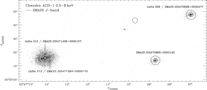
Figure 1: Chandra observation of LkH$\alpha$ 312 on October 18, 2000. The background image is the ACIS-I observation in the energy range 0.5–8 keV of LkH$\alpha$ 312, located at $\sim 8\arcmin$ off-axis (the pixel size is 0$\aas@@fstack{\prime\prime}$25). The color scale is stretched logarithmically to enhance the point spread function (PSF) features, note the $2\arcsec$ asymmetric cusp surrounded by a $10\arcsec$ elliptical halo. The contour map displays arbitrary intensities from the 2MASS $J$-band image using linear scale. The positions of X-ray sources detected above the threshold of $3\,10^{-7}$ are marked with ‘$\times$’. Their infrared positions in the 2MASS survey are marked by ‘+’.

1 Introduction

Since the first X-ray observations of star-forming regions (SFR) with the Einstein Observatory, young PMS low-mass stars, T Tauri stars (TTS), are known to be variable in X-rays (Feigelson & Decampli (1981); Montmerle et al. (1983)). TTS, as active stars, display X-ray flares triggered by magnetic reconnection events occurring in their stellar coronae (see reviews by Feigelson & Montmerle (1999), and Favata & Micela (2003)). The Chandra X-ray Observatory, thanks to its highly elliptical orbit that permits continuous observation over many hours, has collected a real zoo of X-ray flares from TTS in several SFR (e.g., Preibisch & Zinnecker (2002), Feigelson et al. (2002a), Imanishi et al. (2003)). The X-ray flares of TTS are generally impulsive, displaying a fast rise phase ($\sim$2 h) corresponding to a heating phase, followed by an exponential decay corresponding to a cooling phase (e.g., Imanishi et al. (2003)). Only a few long duration flares have been observed from TTS with the previous generation of X-ray satellites, ROSAT and ASCA (SR13, Casanova (1994); objectV773 Tau, Skinner et al. (1997); P1724, Stelzer et al. (1999)). Stelzer et al. (1999) showed that these light curves can be reproduced by the rotational modulation of the exponential decay of a cooling flare. Feigelson et al. (2002a), investigating the variability of young solar-like stars (M_⋆=0.7–1.4 M_⊙) in the Orion Nebula Cloud, find several likely long-duration flares but the low count rates of these events prevent a time-dependent spectroscopy analysis.

M 78 (NGC 2068) is a reflection nebula illuminated by a B1.5V star (HD 38563 North; Mannion & Scarrott (1984)), and located in the northern part of the closest giant molecular cloud, Orion B (L 1630), at a distance of $\sim$400 pc (Anthony-Twarog (1982)). The star-forming region M 78 has been observed with the ACIS-I detector aboard Chandra with 26 h exposure on October 18, 2000 (sequence number 200100). We report here the study of the brightest X-ray source detected during this observation, LkH$\alpha$ 312, located $\sim 10\arcmin$ at the South-East of the optical emission nebula M 78. This source displays an intense X-ray flare with an unusually long rise phase. We describe the ACIS-I data reduction and the X-ray detection of LkH$\alpha$ 312 in §2. The evolutionary status of LkH$\alpha$ 312 is determined from the optical and the NIR data in §3. The Chandra light curve of the flare is presented in §4. The time-dependent spectra is investigated in §5. Finally, the different phases of this flare are discussed in the framework of solar flares in §6. Concluding remarks are presented in §7.

2 Chandra ACIS-I observation

The telemetry format of this observation is ‘Timed Exposure’ with 3.2 s for the frame time, combined with the ACIS mode ‘Faint’. The aimpoint of the ACIS-I detector is $\alpha_{\mathrm{J2000}}=05^{\mathrm{h}}46^{\mathrm{m}}44\aas@@fstack{s}2$, $\delta_{\mathrm{J2000}}=+00\degr 03\arcmin 46\aas@@fstack{\prime\prime}0$ ($l=205.3\degr$, $b=-14.3\degr$), centered on the optical emission nebula M 78.

Table 1: Chandra X-ray sources with 2MASS counterpart in the vicinity of LkH$\alpha$ 312 and their X-ray count rates on October 18, 2000.

CXOU 0547	Count ratea	2MASS J0547	rb	LkH$\alpha$
	[cts ks-1]		[$\arcsec$]
06.9+000047	6.8$\pm$0.3	0696+0000477	0.3	309
08.7+000013	5.7$\pm$0.3	0868+0000140	0.5
14.0+000015	149.8$\pm$1.3	1408+0000157	0.1	312

• In the energy range 0.5–8 keV, from wavdetect taking 93859 s for the exposure.

• Offsets between X-ray and NIR positions.

Following Feigelson et al. (2002b) we start our data analysis from the level 1 processed event list provided by the Chandra X-ray Center (CXC) with the pipeline processing version R4CU5UPD11. We first use the tool acis_process_events of the Chandra Interactive Analysis of Observations (CIAO) package (version 2.2.1 and 2.3) to remove the unnecessary $\pm 0.25\arcsec$ randomization introduced by the pipeline processing on each event position, and we select events belonging to Good Time Intervals (GTI) provided by the CXC. The observation time corrected from deadtime (after each CCD exposure 0.04 s are lost to read the CCD chip) is 93859 s, i.e., more than 26 h. Second we correct the energy and grade of each event using the Penn State’s Charge Transfer Inefficiency (CTI) corrector package (version 1.41; Townsley et al. (2000); Townsley et al. (2002)), which models the CTI characteristics of each CCD chip. The most fundamental result of this CTI correction is the improvement in spectral resolution. Third we clean the data by selecting only events with ASCA grade (0, 2, 3, 4, and 6) and energy in the range 0.5–8 keV after CTI correction. Bad pixels and hot columns are rejected by selecting only events with status bits 1–15 and 20–32 equal to zero. Remaining events with non zero status bits are events which were identified by the pipeline processing as produced by cosmic ray afterglows. However few of them are obvious events from bright X-ray sources misclassified by the pipeline. Hence we reject these events only during X-ray source detection to avoid spurious X-ray sources, but we use them for source spectral analysis. Finally to improve the absolute event positional accuracy, we correct the aspect offset using the fix offsets thread.

Fig. 1 presents an enlargement of the resulting X-ray image at an off-axis angle $\theta\sim 8\arcmin$. Three X-ray sources counterparts of optical emission-line stars (Herbig & Kuhi (1963)) and/or NIR 2MASS sources (all-sky data release; Cutri et al. (2003)) are visible. To obtain accurate X-ray positions and to detect weaker X-ray sources in this area, we use the tool wavdetect of the CIAO package, with the threshold probability of $3\,10^{-7}$, and 11 wavelet scales ranging from $0.5\arcsec$ to $16\arcsec$ in power of $\sqrt{2}$. Table 1 gives the list of the Chandra X-ray sources in Fig. 1 identified with 2MASS counterparts. We find that the agreement between the X-ray and the NIR positions is better than 0$\aas@@fstack{\prime\prime}$5. No X-ray source is detected at the position of LkH$α$ 313, but $4\arcsec$ away we find the remarkable X-ray detection of LkH$α$ 312 with more than 14,000 counts, i.e., an average count rate of $\sim$0.15 cts s^-1.

Table 2: ROSAT/HRI observation of LkH$\alpha$ 312 from September 5 to October 5, 1997.

ROR	Exp.	RX J0547	$\cal L^{\mathrm{a}}$	CRb
2025	[ks]			[cts ks-1]
21h-1	26.7	14.1+000011	213	8.3$\pm$0.7

• $\cal L$ is the likelihood of existence.

• The count rate is for the ROSAT energy band, 0.1–2.4 keV.

Figure 2: ROSAT/HRI X-ray light curve of LkH$\alpha$ 312 obtained from September 5 to October 5, 1997. Crosses show the X-ray light curve and one-sigma error bars in the energy range 0.1-2.4 keV for each observational segment ($\sim$20 min). Background count rates are shown as upper limits when the background subtracted count rate is negative.

We find a previous X-ray detection of this source made from September 5 to October 5, 1997, with the High Resolution Imager (HRI) on board ROSAT in the energy range 0.1-2.4 keV. Table 2 gives the results of our analysis of the archived ROSAT Observation Request (ROR) with the EXSAS package (Zimmermann et al. (1997)). The total exposure of 26.7 ks is the sum of several $\sim 20$ min segment observations spread over one month. We extract source events from the 95% encircled energy radius and produce a background subtracted light curve (corrected from the PSF fraction) with one bintime per segment (Fig. 2). As the HRI has no spectral resolution, we estimate the ROSAT/HRI count rate of the quiescent level with W3PIMMS using the Chandra light curve and spectroscopy results (see low §4 and §5), which give a Chandra quiescent count rate of 0.035 cts s^-1, and a Chandra spectrum model with $N_{\rm H}=1.73\,10^{21}$ cm^-2, $Z\sim 0.2\,Z_{\odot}$, $<kT>$=2.5 keV. We find 0.004 cts s^-1, which is consistent with the low level detected visible in the light curve. This source is clearly variable, however the poor sampling of the light curve precludes obtaining its detailed shape.

3 Evolutionary status of LkH$\alpha$ 312

LkH$\alpha$ 312 was originally selected due to its (weak) H$\alpha$ line emission in slitless grating survey of M 78 (Herbig & Kuhi (1963)). An optical spectrum with 7 Å resolution has been obtained in 1977 by Cohen & Kuhi (1979), leading to its M0 spectral type classification, and its H$\alpha$ equivalent width, EW(H$\alpha$)=8.2 Å (see Table 3). We note that this star is not classified as a TTS in the catalog of Herbig & Bell (1988), probably due to its low EW(H$\alpha$) value. Martín (1997) considers that classical TTS (CTTS) should have EW(H$\alpha$) larger than expected from the average chromospheric activity for their spectral type, and adopts EW(H$\alpha$)=10 Å for early-M stars as a lower limit, instead of the classical EW(H$\alpha$)=5 Å limit. On the basis only of its EW(H$\alpha$), LkH$\alpha$ 312 could then be either an non-accreting PMS star of M 78 or a foreground main-sequence dwarf with H$\alpha$ emission, a dMe star. Of course the detection of the Li I 6707 absorption line would definitively demonstrate the youthfulness of this star, but this observation is not available.

Table 3: Optical and available near-infrared data for the emission line stars discussed in this article. See corresponding $J-H$, $H-K_{\rm S}$ diagram in Fig. 5, spectral energy distributions in Fig. 4, and H.-R. diagram in Fig. 3.

LkH$\alpha$	Cohen & Kuhi (1979)				2MASS					This work
	Spec.	Teff	H$\alpha$	$V$	$J^{\mathrm{a}}$	$H^{\mathrm{a}}$	$K_{\mathrm{S}}$a	$J$-$H$	$H$-$K_{\mathrm{S}}$	AV	Lbolb
#	type	[K]	[$\mathrm{\AA}$]	[mag]	[mag]	[mag]	[mag]	[mag]	[mag]	[mag]	[L⊙]
309⋆	K7	4000	51.2	15.1	11.35$\pm$0.04	10.57$\pm$0.04	10.22$\pm$0.04	0.78$\pm$0.08	0.35$\pm$0.08	2.0$\pm$0.5	1.6$\pm$0.2
312	M0	3917	8.2	15.1	11.32$\pm$0.05	10.52$\pm$0.06	10.12$\pm$0.06	0.80$\pm$0.11	0.40$\pm$0.12	1.8$\pm$0.5	1.5$\pm$0.3
313⋆	M0.5	3802	19.6	15.9	10.75$\pm$0.09	9.79$\pm$0.09	9.23$\pm$0.07	0.95$\pm$0.18	0.57$\pm$0.16	3.5$\pm$0.5	3.9$\pm$0.5

• The errors are the total magnitude uncertainties given at the 90% confidence level.

• From fits of Fig. 4 and taking $d=400$ pc.

• Classified as classical T Tauri star in Herbig & Bell (1988).

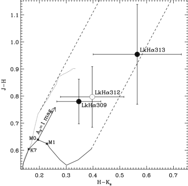
Figure 3: $J-H$, $H-K_{\mathrm{S}}$ diagram of LkH$\alpha$ 312 (open dot). Magnitude error bars are the total magnitude uncertainties at the 90% confidence level. The intrinsic colors of giants (dotted line) and A0–M6 dwarfs (continuous line) from Bessel & Brett (1988), adapted for the 2MASS photometric system using the 2MASS color transformations (Carpenter 2001; Cutri et al. 2003), are plotted for comparison. The extinction law of Cohen et al. (1981), also adapted for the 2MASS photometric system, is drawn for giants and M9 stars. The arrow indicates a visual extinction of 1 mag. Black dots mark the position of known classical T Tauri stars in the vicinity of LkH$\alpha$ 312 (Herbig & Bell 1988).

Figure 4: Spectral energy distributions. The optical spectra and the NIR photometry come from Cohen & Kuhi (1979) and 2MASS, respectively. Dashed line shows the absorbed black body spectrum having the effective temperature found by (Cohen & Kuhi 1979), coinciding with the $J$-band photometry, and consistent with the optical spectra. Upper and lower dotted lines show the same black body spectrum for minus and plus 0.5 mag extinction,respectively. We give the resulting bolometric luminosities, including typical ranges for a typical extinction error of 0.5 mag.

Recently Preibisch & Zinnecker (2002) have shown in the young star cluster IC 348 that H$\alpha$ emission is a poor indicator of circumstellar material around TTS. More precisely, an IR excess in the $L$-band or beyond may be present at the same time as weak H$\alpha$ emission, indicating that such objects are in fact surrounded by a hollow circumstellar disk but currently are accretion quiet. A similar conclusion was drawn by André & Montmerle (1994) based on a sample of $\rho$ Ophiuchi dark cloud’s TTS. Preibisch & Zinnecker (2002) use $K-L$ to trace the infrared excess, but $L$-band photometry is not available for LkH$\alpha$ 312. We have found in the ISO archives, 6.7 $\mu$m and 14.3 $\mu$m ISOCAM detections of the TTS LkH$\alpha$ 313, but the poor angular resolution of ISOCAM ($\sim$6″) cannot resolve the emission of LkH$\alpha$ 312 only $4\arcsec$ away. Fig. 3 displays in a $J-H$, $H-K_{\mathrm{S}}$ diagram the position of two known TTS of M 78 selected due to their strong H$\alpha$ line emission in the vicinity of LkH$\alpha$ 312 (see Table 3). Both TTS have a visual extinction, $A_{\rm V}$, greater than 1 mag. The NIR colors of LkH$\alpha$ 312 are very similar to those of the accreting TTS LkH$\alpha$ 309, and can be retrieved from the intrinsic color of a M0 star by applying $\sim$1.8 mag of visual extinction combined with a small NIR excess, which is maybe produced by a circumstellar disk with an inner hole (André & Montmerle (1994)). This extinction is consistent with LkH$\alpha$ 312 being a young star of M 78 rather than a foreground main-sequence dwarf.

We note that the extinction derived from the color-color diagram for LkH$\alpha$ 312 is a factor of $\sim$4 larger than the one found by Cohen & Kuhi (1979) from optical spectroscopy. The extinction values obtained by Cohen & Kuhi (1979) for LkH$\alpha$ 309 and LkH$\alpha$ 313 are also smaller than the one measured in our color-color diagram. Moreover the bolometric luminosities, $L_{\rm bol}$, given by Cohen & Kuhi (1979) for these objects “represents solely the optical data (extrapolated [with a black body] to infinite wavelength from 0.67 $\mu$m)” (see their Table 5, note of columm 17). To investigate this extinction discrepancy and to udpate the bolometric luminosities, we build spectral energy distributions (SED; Fig. 4). The optical spectra were copied directly from the Fig. 23 of Cohen & Kuhi (1979). The 2MASS photometry was first transformed to the UKIRT system (Carpenter 2001; Cutri et al. 2003), and then converted to flux densities (Cox (2000)). We compute the black body spectrum having the effective temperature found by Cohen & Kuhi (1979), we apply using Fitzpatrick (1999) the extinction given by Cohen & Kuhi (1979), and we scale the absorbed black body spectrum for coincidence with the 0.67 $\mu$m photometry. The obtained SED are far below the NIR data for all the stars of Table 3, hence both the extinction and the bolometric luminosity of Cohen & Kuhi (1979) are underestimated, and need to be udpated. Taking the value found by Cohen & Kuhi (1979) for the effective temperature, we adjust the extinction to obtain an absorbed black body SED, coinciding with the 2MASS photometry in the $J$-band (the contribution of infrared-excess, if any, is negligible at this wavelength), and consistent with the optical spectrum. Fig. 4 displays our best absorbed black body, with the resulting $L_{\rm bol}$ estimate. We consider a typical $A_{\rm V}$ error of 0.5 mag. We list in Table 3 our values of $A_{\rm V}$ and $L_{\rm bol}$ for LkH$\alpha$ 309, LkH$\alpha$ 312, and LkH$\alpha$ 313. The estimated extinctions are now consistent with the ones derived from the color-color diagram.

Fig. 5 shows the H.-R. diagram with the PMS tracks of Baraffe et al. (1998) fitting the Sun (i.e., having the mixing length parameter, $l_{\mathrm{mix}}$, equal to 1.9 times the pressure scale height, $H_{\mathrm{p}}$), with the position of LkH$\alpha$ 312 assuming that LkH$\alpha$ 312 and the other stars of Table 3 are at the distance of M 78 ($d\sim 400$ pc). Considering LkH$\alpha$ 312 as a main sequence star would put it on the 120 Myr isochrone revising down its distance to only $d\sim 90$ pc. This would locate LkH$\alpha$ 312 in the Local Bubble where $N_{\mathrm{H}}\sim 5\,10^{19}$ cm^-2 (Sfeir et al. (1999)). This small distance would not be consistent with the extinction of this object, $A_{\mathrm{V}}\sim 1.8$ mag, which implies $N_{\mathrm{H}}\sim 3.2\,10^{21}$ cm^-2 ( using, e.g., the $N_{\mathrm{H}}/A_{\mathrm{V}}$ conversion factor of Predehl & Schmitt (1995)). Therefore we consider LkH$\alpha$ 312 as a PMS star of M 78.

From the Baraffe et al. (1998) PMS tracks we find that LkH$\alpha$ 312 is located above the 1 Myr isochrone, among known CTTS of M 78, with a stellar mass of 0.7–0.75 M_⊙. We also note that if LkH$\alpha$ 313 were a close binary system the luminosity of the individual components would be decreased by a factor of $\sim$2 (see Fig. 5). In this case LkH$\alpha$ 309, LkH$\alpha$ 312, and LkH$\alpha$ 313 would all be coeval, and LkH$\alpha$ 312 and LkH$\alpha$ 313 would form a gravitationally bound system since their separation is only 4″ on the sky.

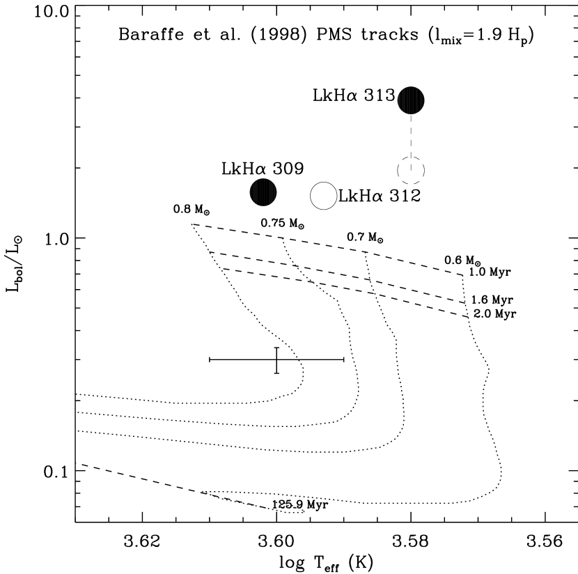
Figure 5: H.-R. diagram of LkH$\alpha$ 312 (open dot). Dotted lines show Baraffe et al. (1998) PMS tracks (with the mixing length required to fit the Sun, $l_{\mathrm{mix}}=1.9\,H_{\mathrm{p}}$, with $H_{\mathrm{p}}$ the pressure scale height). Dashed lines show the corresponding isochrones. Black dots mark the position of known classical T Tauri stars in the vicinity of LkH$\alpha$ 312 (Herbig & Bell 1988). The dashed circle marks the position of LkH$\alpha$ 313 in case of binarity. Error bar shows the typical error on the effective temperature (Cohen & Kuhi 1979), and on the bolometric luminosity (see Fig. 4).

Our final conclusion on the evolutionary status of LkH$\alpha$ 312 is that it is a genuine TTS, with maybe a transition circumstellar disk, belonging to the M 78 star-forming region. Combining $T_{\rm eff}=3917$ K and $L_{\rm bol}=1.5$ L_⊙ leads to the stellar radius $R_{\star}=2.6$ R_⊙.

4 Variability study

4.1 Chandra X-ray light curve

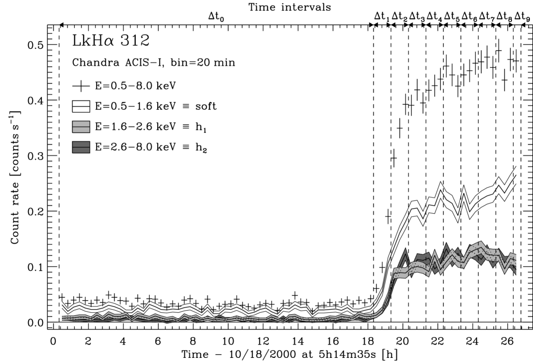
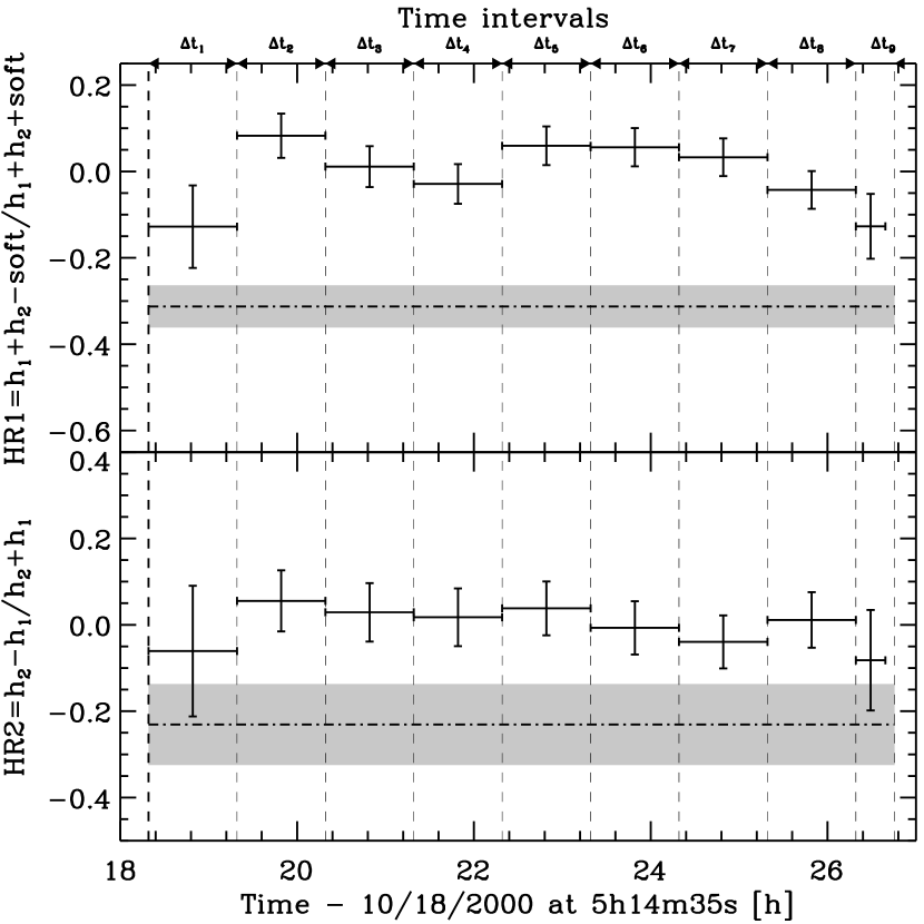
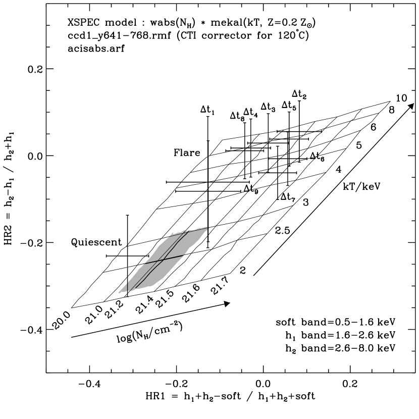
Figure 6: Chandra background subtracted X-ray light curves of LkH$\alpha$ 312. The time binning is 20 min. Crosses show the X-ray light curve and one-sigma error bars in the energy range 0.5-8 keV. The stripes show the X-ray light curves including one-sigma errors corresponding to the energy ranges 0.5–1.6 keV ($soft$ band), 1.6–2.6 keV ($h_{1}$ band), and 2.6–8 keV ($h_{2}$ band). Vertical dashed lines and horizontal arrows define the time intervals, $\Delta$t_i, used for the time-dependent spectroscopy. The quiescent, fast rise, and gradual phases correspond to the time intervals $\Delta$t₀, $\Delta$t₁–$\Delta$t₂, and $\Delta$t₃–$\Delta$t₉, respectively.

Figure 7: Left panel : hardness ratios of LkH$\alpha$ 312 versus time. The top and bottom panels show respectively the hardness ratio $HR1$ and $HR2$, computed from the counts collected in three energy bands ($soft$, $h_{1}$, and $h_{2}$, see Fig. 7), with $1.64\,\sigma$ error bars. The grey stripe indicates the average hardness ratio of the quiescent phase. Right panel : hardness ratios of LkH$\alpha$ 312 compared to spectral models. Iso-energy and iso-absorption lines correspond to absorbed optically thin one-temperature plasma spectra model with 0.2 solar abundances, and show the correspondence between the hardness ratio pair ($HR1$, $HR2$) and the absorption/temperature pair ($N_{\rm H}$, $T$). The grey area shows the average of two plasma temperatures weighted over the emission measure found from spectral fitting of the quiescent phase (see below §5.2, Table 4).

We extract source events from the 99% encircled energy radius, $R(99\%EE)$. We use the empirical fit given by Feigelson et al. (2002b), $R(99\%EE)=8+0.2\,\theta$ (with $\theta$ the off-axis position), which leads for $\theta=8.2\arcmin$ to $R(99\%EE)=9.6\arcsec$. The background is taken from a larger area free of sources. We use the CIAO tool lightcurve, which takes into account Good Time Intervals, to produce background subtracted light curves (corrected from the PSF fraction) with 20 min bintime, and energy filtering.

Fig. 7 shows the light curve of LkH$\alpha$ 312 in the energy range 0.5–8 keV. The X-ray emission was nearly constant during the first 18 h of the observation, defined as the time interval $\Delta$t₀, corresponding to the quiescent phase. The count rate was then multiplied by a factor of 13 during a fast rise phase ($\sim$2 h) corresponding to $\Delta$t₁–$\Delta$t₂, and reached a factor of 16 above the quiescent X-ray level at the end of a gradual phase ($\sim$6 h) showing a slower rise and corresponding to $\Delta$t₃–$\Delta$t₉. The duration of the fast rise phase is similar to the one observed in other TTS (e.g., Imanishi et al. (2003)), however the gradual phase is really unusual. The light curve shape is reminiscent of one of the egress phase of an eclipse; however, as we will see below, this event was triggered by plasma heating. Therefore LkH$\alpha$ 312 displayed a long duration X-ray flare, in contrast to an impulsive flare, during the phase $\Delta$t₁–$\Delta$t₉. Some roughly similar events were already observed by Chandra in the Orion Nebula Cluster (see for example, JW 567 and JW 738 in Fig. 3 of Feigelson et al. (2002a)), or in IC 348 (CXOPZ J034416.4+320955 in Fig. 3 of Preibisch & Zinnecker (2002)) but the X-ray counts were lower, and the datastream was shorter.

The flare count rate was very high, $\sim$0.4–$\sim$0.5 cts s^-1, allowing time-dependent spectroscopy (see §5). To our knowledge this event has the highest count rate observed so far from a PMS low-mass star with Chandra. Such a high count rate implies a pile-up fraction of $\sim$20% for an on-axis source, however for $\theta=8.2\arcmin$ the PSF spreading reduces the pile-up fraction to a value lower than $1\%$ (see The Chandra Proposers’ Observatory Guide), and hence we do not need to worry about this effect in our spectral studies.

4.2 Hardness ratios

Before applying automatic fitting procedures to spectra in §5, we investigate count ratios (‘hardness ratio’ equivalent to ‘X-ray colors’) variation, to assess absorption and/or temperature changes during the flare. We split the 0.5-8.0 keV energy band into three parts : the $soft$ band, the $h_{1}$, and $h_{2}$ hard bands, corresponding to the energy ranges 0.5–1.6 keV, 1.6–2.6 keV, and 2.6–8 keV, respectively. Fig. 7 shows the light curves of these three different bands. The global shape of these light curves is very similar to the full energy band light curve. We compute the following hardness ratios : $HR1\equiv(h_{1}+h_{2}-soft)/(h_{1}+h_{2}+soft)$, and $HR2\equiv(h_{2}-h_{1})/(h_{1}+h_{2})$, with associated errors computed using Gaussian error propagation. The left panel of Fig. 7 shows the flare hardness ratios versus time. They display higher values during the flare phase than during the quiescent phase.

We use rmf and arf files of the quiescent phase of LkH$\alpha$312 (see method to compute these files below §5.1) to simulate with XSPEC synthetic Chandra spectra of absorbed (wabs model with Morrison & McCammon (1983) cross-sections) optically thin one-temperature plasma (mekal model; Kaastra et al. (1996)) with $Z=0.2\,Z_{\odot}$ (found from the spectral fitting of the quiescent phase, see below §5.2 Table 4), for a grid of absorption ($N_{\rm H}$) and temperature ($T$) values, and we compute their corresponding hardness ratios. The right panel of Fig. 7 shows the resulting spectral model grid in the hardness-space with iso-energy and iso-absorption lines. Indeed the energy bands were designed to have the best separation of these iso-energy and iso-absorption lines, which allow a direct correspondence between the hardness ratio pair ($HR1$, $HR2$) and the absorption/temperature pair ($N_{\rm H}$, $T$).

The quiescent phase corresponds in this one-temperature plasma model to $\log N_{\rm H}\sim 20.7$, and $kT\sim 2.7$ keV. However as will be shown below in §5 the quiescent phase is in fact better modeled by a two-temperature plasma. The plasma temperature found with the hardness ratio method is consistent with the average of the plasma temperatures weighted over the emission measures, but the absorption estimate is here clearly underestimated, because as it will see below in §5 (Table 4) the spectral fitting leads to $\log N_{\rm H}=21.2$ with a 90% confidence interval $\log N_{\rm H}$=21.1–21.4. We add in Fig. 7 our best estimate of the ($N_{\rm H}$, $T$) pair for the quiescent phase from our spectral fitting. We can only conclude with these hardness ratios that during the flare the temperature of the plasma increases to $\sim$7 keV on average. There are no variations of the column density.

Table 4: Best fit parameters of the time-dependent spectroscopy with their errors at the 90% confidence levels ($\Delta\chi^{2}$=2.71; corresponding to $\sigma=1.64$ for Gaussian statistics). $\eta\equiv\log{(L_{\mathrm{X,intr}}/L_{\mathrm{bol}})}$.

				Temperature		Emission Measure				$\log L_{\mathrm{X,intr}}$	$\eta$
$\Delta$ti	$N$	$N_{\mathrm{H,21}}$	$Z$	$kT_{\mathrm{low}}$	$kT_{\mathrm{high}}$	$EM_{\mathrm{low}}$	$EM_{\mathrm{high}}$	$\chi^{2}_{\nu}$ ($\nu$)	$\cal{Q}$	0.5–2/2–8/0.5–8
	[cts]	[cm-2]	[$Z_{\odot}$]	[keV]		[$10^{54}$ cm-3]			[%]	[erg s-1]
0	2207	1.7${}_{-0.5}^{+0.6}$	0.2${}_{-0.1}^{+0.2}$	1.0${}_{-0.1}^{+0.2}$	3.1${}_{-0.6}^{+1.8}$	0.2${}_{-0.1}^{+0.4}$	0.5${}_{-0.2}^{+0.1}$	1.08 ( 79)	29	30.6 30.4 30.8	-2.9
1	392	1.2${}_{-1.2}^{+1.3}$	0.2${}_{-....}^{+1.1}$		4.6${}_{-1.4}^{+3.1}$		1.9${}_{-0.6}^{+0.6}$	1.04 ( 14)	41	31.0 31.1 31.4	-2.4
2	1195	2.4${}_{-0.7}^{+0.7}$	0.5${}_{-....}^{+1.6}$		6.9${}_{-1.7}^{+3.3}$		5.8${}_{-1.4}^{+1.1}$	1.14 ( 48)	23	31.5 31.8 32.0	-1.8
3	1394	1.9${}_{-0.6}^{+0.7}$	2.1${}_{-1.4}^{+3.9}$		6.4${}_{-1.4}^{+1.8}$		5.0${}_{-1.8}^{+1.5}$	1.15 ( 54)	21	31.6 31.9 32.0	-1.7
4	1493	1.7${}_{-0.6}^{+0.6}$	0.5${}_{-0.4}^{+0.6}$		5.6${}_{-1.1}^{+1.6}$		6.9${}_{-1.0}^{+1.1}$	0.68 ( 57)	97	31.6 31.8 32.0	-1.7
5	1561	2.2${}_{-0.5}^{+0.6}$	0.0${}_{-....}^{+0.4}$		7.6${}_{-1.7}^{+3.2}$		8.0${}_{-0.8}^{+0.7}$	0.85 ( 63)	80	31.6 31.8 32.1	-1.7
6	1590	2.8${}_{-0.6}^{+0.6}$	0.1${}_{-....}^{+0.3}$		5.3${}_{-1.0}^{+1.5}$		9.0${}_{-1.0}^{+1.1}$	0.86 ( 61)	77	31.7 31.8 32.1	-1.7
7	1642	2.1${}_{-0.5}^{+0.6}$	0.5${}_{-0.4}^{+0.4}$		5.1${}_{-0.8}^{+1.2}$		7.8${}_{-0.9}^{+1.0}$	1.06 ( 62)	36	31.7 31.8 32.1	-1.7
8	1641	2.1${}_{-0.5}^{+0.5}$	0.1${}_{-....}^{+0.3}$		4.8${}_{-0.8}^{+1.1}$		8.6${}_{-1.0}^{+1.1}$	1.11 ( 62)	26	31.7 31.8 32.0	-1.7
9	715	1.6${}_{-0.8}^{+0.9}$	0.0${}_{-....}^{+0.4}$		3.8${}_{-0.8}^{+1.2}$		9.1${}_{-1.7}^{+1.8}$	0.56 ( 28)	97	31.7 31.7 32.0	-1.8
1–9	11327	2.6${}_{-0.3}^{+0.4}$	0.3${}_{-0.1}^{+0.1}$	0.8${}_{-0.4}^{+0.5}$	5.1${}_{-0.4}^{+0.5}$	0.3${}_{-0.2}^{+0.3}$	7.4${}_{-0.3}^{+0.3}$	1.09 (227)	17	31.6 31.8 32.0	-1.7

5 Time-dependent spectroscopy

5.1 Methodology

The spectral analysis is performed with XSPEC (version 11.2). Plasma models are convolved with the response matrix file (rmf) describing the spectral resolution of the detector as a function of energy, and an auxiliary response file (arf) describing the telescope and ACIS detector effective area as a function of energy and location in the detector. Reduction in exposure times due to telescope vignetting, and possible bad CCD columns moving on the source with satellite aspect dithering, is included in the arf file. We use the rmf files and the quantum efficiency uniformity (QEU) files provided with the CTI corrector package. These QEU files are used by mkarf to generate arf file consistent with our CTI corrected events. We note that for LkH$\alpha$ 312 (I1 chip, row 749) far away from the readout node (I1 chip, row 1), the CTI correction improves the energy resolution from FWHM$\sim$130 eV to 110 eV in the soft part of the spectrum, and from FHWM$\sim$260 eV to 190 eV in the hard part of the spectrum (see Townsley et al. (2002)). We apply the acisabs model to the arf file to take into account the contamination of the ACIS optical blocking filter. For our observation 453 days after launch, this correction is negligible above $\sim$1 keV, but leads to a decrease of 20% of the effective area at 0.5 keV, which is not negligible to determine an accurate value of hydrogen column density on the line of sight. Best-fit model parameters are found by comparing models with the pulse height distribution of the extracted events using $\chi^{2}$ minimization. The source spectrum is rebinned with grppha in the ftools package to a minimum of 20 source counts per spectral bin. The model is improved until obtaining $\chi^{2}_{\nu}\sim 1$ and ${\cal Q}\geq 5\%$, with $\chi^{2}_{\nu}$ the reduced $\chi^{2}$ (i.e., $\chi^{2}$ over the degree of freedom, $\nu$), and ${\cal Q}$ the probability that one would observe $\chi^{2}_{\nu}$, or a larger value, if the assumed model is true, and the best-fit model parameters are the true parameter values. The parameter error at the 90% confidence level ($\Delta\chi^{2}$=2.71; corresponding to $\sigma=1.64$ for Gaussian statistics) is computed with the commands error and steppar.

5.2 Multi-temperature plasma model

We first model the plasma in XSPEC with an optically thin single-temperature plasma model (mekal model; Kaastra et al. (1996)), combined with photoelectric absorption using Morrison & McCammon (1983) cross-sections (wabs model). We are led to increase the number of plasma component to improve the goodness-of-fit.

5.2.1 Quiescent emission and flare spectra

Fig. 8 shows the quiescent and the flare spectra for comparison. Both phases require more than a one-temperature plasma model to be fitted, and we use a two-temperature model. The resulting fit parameters are listed in Table 4. The quiescent spectrum is featureless, no emission lines are visible. Approximatively 70% of the X-ray emission comes from a high temperature plasma at energy $kT=3.1$ keV. The plasma abundance is $Z\sim 0.2\,Z_{\odot}$ (this is the value that was used previously for hardness ratio study in §4.2). The average plasma energy, weighted over the emission measure, is $<kT>$=2.5 keV, corresponding to an average temperature of 29 MK, similar to the temperature found in the previous section with the hardness ratio method. The absorption is low with $N_{\rm H}=1.3$–$2.3\,10^{21}$ cm^-2 corresponding to $A_{\rm V}\sim$0.7–1.3 mag (Predehl & Schmitt (1995)).

The intrinsic luminosity in the energy range 0.5–8 keV is $L_{\rm X,intr}=6\,10^{30}$ erg s^-1. From the stellar radius $R_{\star}=2.6\,R_{\odot}$ inferred from the H.-R. diagram (see above §3), we find a high X-ray stellar flux, $F_{\rm X}=1.4\,10^{7}$  erg cm^-2 s^-1. To quantify the X-ray activity we use the logarithm of the ratio of the X-ray luminosity corrected from absorption on the bolometric luminosity, $\eta\equiv\log(L_{\rm X,intr}/L_{\rm bol})$. (This indicator is independent of the source distance.) The quiescent phase displays $\eta=-2.9$. This value is very high compared with the average value for TTS, $\eta\sim-4$, and implies that the corona of LkH$\alpha$ 312 reached the saturation  level.

Figure 8: Chandra ACIS-I spectra of LkH$\alpha$ 312. The upper panel displays separately the ACIS-I data for the quiescent (circle mark) and flare phases. The lines are the corresponding models, a two-temperature plasma combined with photoelectric absorption (see Table 4 for details). The lower panel shows the residual $\chi$ of the modeling.

The large number of events collected during the flare phase (about 12,000) unveils in the flare spectral residual a pseudo-absorption line at 1.785 keV, which is due to a calibration problem of the quantum efficiency just below the Si absorption edge at 1.839 keV. We suppress the corresponding energy channels for the flare phase fitting, which improves greatly the goodness-of-fit. This calibration problem is not visible in spectra with only a few thousand counts, and we will neglect it in §5.2.2. The flare spectrum is also nearly featureless, with only the He-like line of the Fe XXV visible at 6.7 keV. Approximatively 95% of the X-ray emission comes from a high energy plasma at $kT=5.1$ keV. We detect a lower energy plasma, which is similar to the one found during the quiescent phase, with $kT\sim 1$ keV and $EM\sim 0.2\,10^{54}$ cm^-3. The flare abundance is also comparable with the quiescent one; we detect no metallicity enhancement as found in the bright X-ray flares of active stars (e.g., Güdel et al. (2001)). We obtain during the flare phase an accurate measurement of the absorption, $N_{\rm H}=2.3$–$3.0\,10^{21}$ cm^-2 corresponding to $A_{\rm V}\sim$1.3–1.7 mag (Predehl & Schmitt (1995)), which is consistent with the optical extinction obtain previously from SED in §3.

Thanks to the high count rate of this flare we can make a time-dependent spectroscopy of the rise phase to investigate the physical properties of this event.

Figure 9: Time-dependent flare spectra. Time interval spectra are plotted from bottom to top with their one-temperature fit (see Table 4 for details) multiplied by an arbitrary constant.

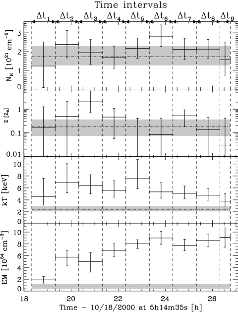
Figure 10: Flare parameters versus time (crosses) compared with the quiescent preflare values (grey stripes) from values in Table 4. The measured values for the quiescent phase are indicated with a dashed-dot line, with a range shown as a grey stripe. Time sampling is defined in Fig. 7. Since the flare spectra can each be fitted with a single temperature, we take for comparison with the quiescent preflare temperature the average of the two plasma temperatures weighted over the emission measures, and for the quiescent preflare emission measure the sum of the two emission measures.

5.2.2 Time-dependent spectroscopy of the flare phase

Fig. 9 shows the flare spectra for the time intervals $\Delta\mathrm{t}_{1}$–$\Delta\mathrm{t}_{9}$, which all have a duration of 1 h at the exception of the shorter interval $\Delta\mathrm{t}_{9}$ having only about 25 min. This bin selection is a compromise between larger bins, which would smooth short term phenomena, and shorter bins, which would reduce the number of count. One-hour bins are long enough here to collect $\sim$1,500 counts and hence have enough statistics to derive accurate physical parameters. The spectra are featureless, there is not enough statistics to detect the 6.7 keV iron line, which becomes appearent only by adding all these time intervals (see Fig. 8). We find a reliable fit only with a high temperature plasma. We tried to add a low temperature plasma having the same properties than the one found during the quiescent state, but this did not improve significantly the fitting result. The X-ray emission of the flare plasma is hence dominated by this high temperature component. However as we saw previously in §5.2.1 by adding all the flare time intervals, it is possible with enough statistics to constrain this low temperature emission. We list all the fit parameters in Table 4.

Fig. 10 plots the flare spectral parameters with their errors at the 90% confidence level versus time compared to their quiescent values. The absorption is consistent during the flare with its quiescent value. The plasma abundance is also consistent during the flare with its quiescent value with maybe the exception of the interval $\Delta\mathrm{t}_{3}$ where the metallicity is increased by a factor of 10. This metallicity enhancement could be explained by photospheric evaporation produced by the flare as seen in active stars (e.g., Güdel et al. (2001)). However assuming that the metallicity keeps its quiescent value during the flare, this deviant bin is consistent with being a statistical fluctuation, as in 10 independent measurements one discrepant value is expected at the 90% confidence level. The emission measure increases until $\Delta\mathrm{t}_{6}$, and saturates.

The emission measure behaviour is hence totally different from a rotational modulation of a flare decay (Stelzer et al. (1999)), where the emission measure decreases exponentially. The plasma temperature is greater than the average quiescent temperature during all the flare, and reaches its maximum for $\Delta\mathrm{t}_{5}$ with $kT=7.6$ keV. We will consider this maximum as the peak flare in the following section. The temperature interval $\Delta\mathrm{t}_{5}$–$\Delta\mathrm{t}_{9}$ is reminiscent of the cooling phase of an impulsive flare, which displays both an exponential decrease of the temperature and the emission measure, however here no decay is visible for the emission measure.

The luminosity in the energy range 0.5–8 keV corrected for absorption is $L_{\mathrm{X,intr}}\sim 1\times 10^{32}$ erg s^-1 throughout nearly all the flare. The X-ray luminosity of the flare peak reaches $\sim$2% of the stellar bolometric luminosity. The total energy released by this flare is $E_{\mathrm{X}}=7.2\,10^{33}$ erg in 8.5 h.

6 Discussion

The LkH$\alpha$ 312 flare detected here is extraordinary in its X-ray luminosity and, due to the serendipitous nature of the off-axis location, in the quality of the X-ray data. It thus provides a valuable opportunity to examine the applicability of established theories for solar-type magnetic reconnection flaring in the limit of high power and long duration. Note that we consider the absorption, consistent with a constant value of $N_{\mathrm{H}}\approx 1.7\,10^{21}$ cm^-2, to be external to the flare environment and of no interest here.

6.1 Quiescent emission

The low X-ray emission prior to a major flares, such as we see in the first 5 hours of the $Chandra$ observation, is usually considered to be a ‘quiescent’ plasma component distributed over large regions as in the solar corona. But the quiescent emission here is much hotter and more luminous than the solar corona, with the bulk of temperatures ranging from 10–35 MK with an average (weighted over the emission measure) of 29 MK (see §5.2.1, Table 4). In contrast, the non-flaring solar corona has average (weighted over the emission measure) temperature of $\sim 2$ MK (Peres et al. (2000)). The intrinsic quiescent X-ray luminosity in LkH$\alpha$ 312 is $6\,10^{30}$ erg s^-1 in the Chandra band (0.5–8 keV) and probably $\sim 10^{31}$ erg s^-1 in a full bolometric X-ray band. In contrast, the bolometric X-ray luminosity of the non-flaring solar corona is only $3\,10^{27}$ erg s^-1 during solar minimum to $3\,10^{28}$ erg s^-1 during solar maximum (Peres et al. (2000)). Note that the surface area of LkH$\alpha$ 312 is only 6.8 times that of the Sun (see §5.2.1), so the X-ray luminosity difference of a factor of order 1,000 cannot be attributed to a larger surface area.

The higher temperature of the LkH$\alpha$ 312 quiescent X-ray emission could be attributed to enhanced coronal processes. Theories for solar coronal heating based on the release of magnetic energy (Parker (1979); Parker (1988); Priest & Forbes (2000)) have $kT\simeq f\,B^{2}/(8\pi\,n_{\mathrm{c}})$, where $n_{\mathrm{c}}$ is the coronal electron density and $f$ is the fraction of the coronal magnetic field which is converted into heat. A 4-fold increase on average magnetic field strength, for example, could account for the temperature difference. But it seems unlikely that the enormous difference in luminosities can be explained in this fashion. Since $L_{\mathrm{X,quiescent}}\propto n_{\mathrm{c}}^{2}\,V_{\mathrm{c}}$ where $V_{\mathrm{c}}$ is the coronal volume, and since $n_{\mathrm{c}}$ cannot be significantly raised without lowering the temperature, a $\sim 10^{3}$ increase in coronal volume would have to be present to give the $10^{31}$ erg s^-1 quiescent luminosity. The corona would have to extend $>$10 stellar radii without significant density decrease, which seems quite unrealistic. Alternatively the X-ray volume filling factor in the corona of LkH$\alpha$ 312 could be 1,000 times higher than in the solar corona.

The quiescent emission may also arise from the sum of many eruptive flares while not excluding a contribution from coronal heating processes. This is suggested by the growing evidence for microflaring as the origin of most of the quiescent X-ray emission from magnetically active stars (Güdel et al. (2003), and references therein). At least 10 flares each with $L_{\mathrm{X,flare}}\leq 10^{30}$ erg s^-1 must continuously be active over the stellar surface. The lack of variation in flux or temperature during the quiescent phase suggests a large number of small and moderate-sized flares are present, which in turn suggests a dense coverage of the stellar surface with high-strength magnetic fields and hence a high surface filling factor. This is consistent with the fact that the quiescent X-ray luminosity is found to reach the saturation level as shown in §5.2.1.

As the quiescent level appears remarkably stable and bright, our understanding of the strong microflaring of LkH$\alpha$ 312 could be advanced by a follow-up X-ray observation with high spectral resolution. In particular, the density of the flare plasmas can be estimated using He-like line ratios. Ne IX at 0.92 keV is sensitive to densities from a few $10^{10}$ to a few $10^{12}$ cm^-3 (Porquet & Dubau (2000)). However, the ionization fraction of Ne IX may be low due to the high temperatures : only 0.4% for plasma at $kT$=1 keV and 0.007% at 3 keV (Arnaud & Rothenflug (1985)). Mg XI at 1.34 keV with a ionization fraction of 6.8% at $kT$=1 keV should then be easier to detect, but it probes only higher density from a few $10^{11}$ to a few $10^{13}$ cm^-3 (Porquet & Dubau (2000)). While the current mission gratings with CCD detectors are maybe not sufficiently sensitive for this investigation, it will be possible with the forthcoming X-ray spectrometer aboard ASTRO-E2, a next generation instrument using X-ray bolometers.

6.2 Rise phase

The morphology of the LkH$\alpha$ 312 flare rise is distinctively slow ($\tau\simeq 120$ min) in contrast to a typical solar flare rise ($\tau_{\odot}\simeq 5$ min), and smooth with no precursors, shoulders or secondary events. The smoothness may indicate a relatively simple magnetic geometry such as a single bipolar loop or bipolar loop arcade without adjacent multipolar magnetic areas. The scale length of the loops can be tentatively constrained by assuming that the magnetic structure confining the X-ray emitting plasma is stable during the slow and smooth rise. Loops suffer magnetohydrodynamical instabilities with characteristic growth timescale, $\tau$, corresponding to the length scale of the pre-eruption region, $l$, divided by the ambient Alfvèn speed (Priest & Forbes (2000)), $V_{\mathrm{A}}\propto B\,n_{\mathrm{c}}^{-1/2}$, with $B$ the average magnetic field strength, and $n_{\mathrm{c}}$ the pre-flare coronal density. We scale the LkH$\alpha$ 312 values to the solar values : $l_{\odot}=5\,10^{10}$ cm for an average CME (Gilbert et al. (2001), and references therein), $B_{\odot}\sim 100$ G (e.g., Parker (1988)), and $n_{\mathrm{c,\odot}}\sim 10^{9}$ cm^-3 (see Shibata & Yokoyama (2002), and references therein). We obtain :

$$l=l_{\mathrm{\odot}}\,(\tau/\tau_{\odot})\,(B/B_{\odot})\,(n_{\mathrm{c}}/n_{\mathrm{c,\odot}})^{-1/2}\,.$$ (1)

We point out that this scale length is the scale for the volume of erupted field. Generally, it can be larger than the volume from which the X-ray emission arises, and in the case of the solar flares the scale length of the erupted region may be 2 to 3 times greater than the scale of the flaring region. Therefore we estimate the following upper limit for the height, $h$, of a semi-circular magnetic loop filled by the X-ray emitting plasma :

$$h_{\mathrm{max}}=0.5\times l/3\,,$$ (2)

$$h_{\mathrm{max}}=2\,10^{11}\,\mathrm{cm}\times(B/100\,\mathrm{G})\,(n_{\mathrm{c}}/10^{9}\,\mathrm{cm^{3}})^{-1/2}\,.$$ (3)

Replacing the loop height by the loop half-length, $L=\pi\,h/2$, leads to the following constraint :

$$L\leq 10^{8}\,\mathrm{cm}\times B\,n_{\mathrm{c,12}}^{-1/2}\,.$$ (4)

This formula will be used in the next section combined with an estimate of $L$ and $B$, to derive a lower limit estimate of the pre-flare coronal density.

6.3 Peak properties

Both X-ray (Favata & Micela (2003)) and radio (Güdel (2002)) stellar peak flare properties show that magnetic loop scaling relationships can be derived from the corresponding solar flare properties. We use here the work of Shibata & Yokoyama (1999, 2002) which is based on a scaling law relation for the maximum temperature of reconnection heated plasma and magnetic field strength derived from MHD simulations (Yokoyama & Shibata 1998, 2001). We note, however, that this work is based on MHD simulations where the effect of the radiative cooling can be neglected, so scaling laws which include the cooling switching from conductive to radiative as time proceeds (Cargill et al. (1995)) have not yet been numerically tested.

The theory of Shibata & Yokoyama involves a roughly semi-circular magnetic loop with half-length $L$, magnetic field $B$, and electron density after chromospheric evaporation $n_{\mathrm{e}}$. These parameters are derived from the peak X-ray temperature and emission measure together with prior knowledge of the pre-flare coronal electron density $n_{\mathrm{c}}$, using the following scaling formulae where $kT$ is expressed in keV :

$$L=2\,10^{11}\,\mathrm{cm}\times EM_{54}^{3/5}\,kT^{-8/5}\,n_{\mathrm{c,12}}^{-2/5}\,\rm,$$ (5)

$$B=32\,\mathrm{G}\times EM_{54}^{-1/5}\,kT^{17/10}\,n_{\mathrm{c,12}}^{3/10}\,\rm,$$ (6)

$$n_{\mathrm{e}}=10^{10}\,\mathrm{cm}^{-3}\times EM_{54}^{-2/5}\,kT^{12/5}\,n_{\mathrm{c,12}}^{3/5}\,\rm.$$ (7)

The loop parameters are hence function of $n_{\mathrm{c,12}}$, which can be constrained. First, for consistency with the chrosmospheric evaporation assumption, the flare coronal density must be lower than the pre-flare coronal density, which leads using (7) to the following upper limit estimate for $n_{\mathrm{c,12}}$ :

$$n_{\mathrm{c,12}}\leq 10^{-5}\,EM_{54}^{-1}\,kT^{\,6}\,\rm.$$ (8)

Second, from (4) and using (5)–(6) leads to a lower limit on $n_{\mathrm{c,12}}$ :

$$n_{\mathrm{c,12}}\geq 10^{9}\,EM_{54}^{4}\,kT^{-33/2}\,.$$ (9)

As the LkH$\alpha$ 312 peak flare values ($EM_{54}=8.0$ and $kT=7.6$ keV) are consistent with the empirical correlation (see Fig. 1 of Shibata & Yokoyama (2002)), no special scaling laws are required for this flare. Applying the previous set of formulae, we find :

$$0.01\leq n_{\mathrm{c,12}}\leq 0.24\,\rm,$$ (10)

$$L=2.3\,10^{10}\,\mathrm{cm}\times n_{\mathrm{c,12}}^{-2/5}\,\rm,$$ (11)

$$B=670\,\mathrm{G}\times n_{\mathrm{c,12}}^{3/10}\,\rm,$$ (12)

$$n_{\mathrm{e}}=6.4\,10^{11}\,\mathrm{cm}^{-3}\times n_{\mathrm{c,12}}^{3/5}\,.$$ (13)

Numerically, we find that the loop half-length ranges from 4.8–16$\,10^{10}$ cm (0.3–0.9 R${}_{\star})$, the loop height ranges from 3.1–10$\,10^{10}$ cm (0.2–0.5 R_⋆, i.e., 0.5–1.3 R_⊙), the magnetic field from 430–180 G, and the flare loop densities from 2.4–0.4$\times 10^{11}$ cm^-3.

6.4 Gradual phase and decay phase

The gradual phase, which has a slower rise and follows the fast rise phase, is really unusual. It may be explained by the rapid fall of the stellar magnetic field with height. Indeed in this situation when the magnetic loop system rises, the reconnection site is continually moving up into a weaker field region, which produces the decline of the rate of magnetic energy release.

Much of solar and stellar flare loop modelling is based on the decay phase of the flare when the loop plasma is cooling (see review by Reale (2002); e.g., Reale et al. (1997)). Unfortunately, only the beginning of this phase may have been observed in LkH$\alpha$ 312 in the second part of the gradual phase where we find a decrease of the plasma temperature from 88 MK (7.6 keV) to 44 MK (3.8 keV) over 5 hours using one-hour averaged spectra (Figure 10). However during this period, the broad-band luminosity remained constant, which is rather unusual for a cooling period, so that the emission measure (density and/or volume) increased somewhat as the plasma cooled, or short heating phases may occur which are smoothed by the averaged spectra.

7 Conclusions

So far, LkH$\alpha$ 312 was considered from $\sim$30-yr old H$\alpha$ prism surveys as an unremarkable, weak-activity star at the periphery of M 78, until Chandra unveiled its extraordinary activity in X-rays. Our study based on the available optical and IR data shows that it is likely a $<1$ Myr-old T Tauri star similar to the Sun ($M_{\star}\sim 0.7$–0.75 M${}_{\odot},R_{\star}\sim 2.6$ R_⊙), about as luminous ($L_{\mathrm{bol}}\sim 1.5$ L_⊙), and surrounded by a hollow circumstellar disk. It is therefore perhaps a transition object between an active accreting ‘classical’ T Tauri star, and a genuine disk-free ‘weak-line’ T Tauri star.

In contrast with these fairly unoriginal properties of LkH$\alpha$ 312, our Chandra observations revealed a particularly long and intense X-ray flare, in addition to a bright quiescent emission. Because of the intensity of the flare ($\sim 0.5$ Chandra cts s^-1) and its favorable far off-axis position on the ACIS-I detector which prevented pile-up, the quiescent state as well as the rise phase of the flare could be studied at an unprecedented level of detail, yielding spectroscopy resolved on a time scale of down to 1 h out of a 26 h-long observation. The flare itself is quite remarkable, with its high X-ray luminosity (comparable to that of only a handful of TTS so far) and slow rise, but so is the level of the quiescent emission, which is saturated. The high intensity of the quiescent level was already perceptible in the ROSAT/HRI observation of 1997, so it is likely not a brief, transient phenomenon.

Quantitatively, the X-ray properties derived from our Chandra observations are as follows : (i) the quiescent emission of LkH$\alpha$ 312 is stable over 18 h of observation and saturated at a high level of activity ($L_{\mathrm{X}}/L_{\mathrm{bol}}\sim 10^{-3}$, with $L_{\mathrm{X}}\sim 6\times 10^{30}$ erg s^-1); (ii) LkH$\alpha$ 312 also displayed an unusually long and intense X-ray flare, showing a long rise phase extending over several hours. This flare was bright, reaching $L_{\mathrm{X}}\sim 10^{32}$ erg s^-1, i.e., $\sim$2% of the bolometric luminosity. Perhaps more remarkably, the peak temperature was quite high ($kT\sim 7$ keV). (iii) In terms of solar-type magnetic confinement of the plasma, the application of the scaling laws found by Shibata & Yokoyama shows that the flare corresponds to a fairly large volume (maximum height of about 1 R_⊙), and typical solar coronal densities ($\sim 10^{11}\,{\rm cm}^{-3}$).

The problem is to understand the reasons for these rather extreme X-ray properties, both in the quiescent state and in the flaring state. The first, “standard” way is to address the problem in the framework of solar physics. This is how we derived the flare properties (size and density of the confining magnetic loop, strength of the magnetic field). As discussed in §6.1, one could invoke enhanced coronal processes and/or microflaring, 1,000 times more intense than the quiet Sun, or a volume filling factor in the LkH$\alpha$ 312 corona 1,000 times larger than in the solar corona, but the physical reasons for such an enhancement are unclear. This is in fact a general problem for pre-main sequence stars : the mechanism for magnetic field generation leading to the high level of X-ray activity is still not well understood. For instance, the lack of an X-ray luminosity/rotation correlation on large samples like in Orion is perhaps due to the fact that an $\alpha^{2}$ (turbulent) dynamo operates at the young TTS stage, as opposed to the standard rotation-convection induced $\alpha-\omega$ dynamo which holds in late-type main-sequence stars (Feigelson et al. (2003)).

An alternative way is to consider that the enhanced X-ray activity of LkH$\alpha$ 312, and perhaps more generally of at least some other, very X-ray luminous TTS, is triggered by an external cause such as a close, faint companion like a brown dwarf or even a planet. Indeed, as shown by Cuntz et al. (2000), planets can cause enhanced magnetic activity if they are sufficiently massive and close to the parent star, like 51 Peg-like planet-bearing stars. The general idea is that tidal effects can enhance the dynamo by altering the outer convective zone, and/or, if the planet is magnetized, the star and the planet can interact magnetically via shearing and reconnections, for instance as in the star-disk magnetic interaction mechanism proposed by Montmerle et al. (2000) to explain the triple X-ray flare of the YLW15 protostar. In such a framework, the rotation information would be important : although a slow rotation would not be conclusive, a fast rotation (periods of days or less) could be indicative of a tidally locked, RS CVn-like binary system. We note that the circumstellar disk of LkH$\alpha$ 312 is hollow, with no accretion taking place, which is indeed consistent with the possible presence of a planet clearing the inner disk (e.g., Nelson (2003)).

Both ground and space follow-up observations will be needed to investigate the coronal properties of LkH$\alpha$ 312 as a genuine TTS and its influence on its circumstellar material : medium resolution optical spectroscopy, to confirm its youthfulness with Li I 6707 absorption line measurement, to check that the H$\alpha$ emission has not changed, and to estimate its projected equatorial velocity; to determine its rotational period from the photometric modulation of starspots; high-resolution IR spectroscopy to detect the possible presence of a very low mass companion; near-IR high resolution imagery to study a possible transition circumstellar disk; and of course high resolution X-ray spectroscopy to probe the density of its coronal plasma.