Cosmic Microwave Background Polarization: constraining models with a double reionization

Neutral hydrogen around high–$z$ QSO and an optical depth $\tau\sim 0.17$ can be reconciled if reionization is more complex than a single transition at $z\simeq 6-8$. Tracing its details could shed a new light on the first sources of radiation. Here we discuss how far such details can be inspected through planned experiments on CMB large-scale anisotropy and polarization, by simulating an actual data analysis. By considering a set of double reionization histories of Cen (cen (2003)) type, a relevant class of models not yet considered by previous works, we confirm that large angle experiments rival high resolution ones in reconstructing the reionization history. We also confirm that reionization histories, studied with the prior of a single and sharp reionization, yield a biased $\tau$, showing that this bias is generic. We further find a monotonic trend in the bias for the models that we consider, and propose an explanation of the trend, as well as the overall bias. We also show that in long-lived experiments such a trend can be used to discriminate between single and double reionization patterns.

1 Introduction

The first–year WMAP data release detected a strong anisotropy–polarization cross–correlation at low $l$ (Kogut et al.  wmap:kogut (2003)). Previous analyses suggested that the Intergalactic Medium (IGM) had reionized at a redshift $z\simeq 6$–8, and led one to expect an optical depth for Thomson-scattering $\tau\la 0.05$ (Miralda–Escudè  mira (2003)). Observations of the Gunn-Peterson effect in high–$z$ QSO, requiring a fraction of neutral hydrogen at $z\sim 6$–7, agreed with this scheme (Djorgovski et al. djor (2001), Becker et al. becker (2001); see however Malhotra & Rhoads malho (2004)). On the contrary, the level of anisotropy–polarization correlation, in WMAP data, indicates $\tau\approx 0.17$ (Kogut et al. wmap:kogut (2003)) and reionization at $z\ga 16$, assuming a single-step reionization model. If so, the reionization history could have been quite complex. In turn, data on CMB anisotropy and polarization could shed new light on the birth and evolution of primeval objects

Different options on the nature of primeval objects have been considered. Ciardi et al. (ciardi (2003)) showed that metal–free stars in early galaxies may account for a depth up to $\tau\approx 0.15$, although this seems an upper limit to such a picture (Ricotti & Ostriker 2004a ). Various authors also considered an early pre-ionization due to black holes in small galaxies (Ricotti & Ostriker 2004b ) or miniquasars (Madau et al. madau (2004)), or even the effects of sterile neutrino decay (Hansen & Haiman haha (2004)).

Independently of the ionizing mechanism, however, comparing WMAP and QSO data suggests that reionization is not achieved in a single, rapid step, but involves at least two different stages. Double reionization models were suggested, even before WMAP, by Cen (cen (2003)), Wyithe et al. (wsl (2003) ), Sokasian et al. (soka (2004)), Ricotti & Ostriker (2004a ) and others. In these models the ionization fraction attains a value $x_{e}\approx 1$, at some high $z$, then partial recombination occurs, while a second reionization takes place at $z=6$–8 and then $x_{e}=1$ (for discussion purposes, we neglect Helium ionization).

Haiman & Holder (haho (2003)) also considered another option, that the Universe partially reionized (up to $x_{e}\sim 0.5$–0.8) at a high $z_{r}$, to achieve a complete reionization at $z\simeq 6$–8. A similar 2–step reionization was also schematically considered by Kaplinghat et al. kap (2003), for its effects on CMB. Still different reionization patterns were treated by Bruscoli et al. (bruscoli (2002)), Hu & Holder (huho (2003) ), Naselsky & Chiang (nachiang (2004)) and Colombo (colombo (2004)), confirming the interest in the relation between CMB data and early reionization, although often specifying no link with early object formation models. The present work is based on the dependence of the low–$l$ behavior of the $C_{l}^{E}$ spectra on the whole reionization history, and aims to predict the actual detectability of $\tau$, as well as of the reionization redshift(s), the ionization rate(s), etc., with data on large angular scales. When dealing with full–sky small–angle experiments, the high number of pixels forces one to work in harmonic space which, under the assumption of a Gaussian signal, allows a fair information compression. For large–angle data, working directly in pixel space, as opposed to harmonic space, is numerically feasible and allows one to take into account a number of features that experiments can hardly avoid.

In particular, the actual CMB signal can be recovered only on a portion of the celestial sphere. An example of such a limitation is the effect of Galactic contamination, making anisotropy data unreliable within $\sim 20\degr$ of the galactic plane. On the other hand, first year WMAP data indicate that the main polarized foreground at frequencies up to 70 GHz is Galactic synchrotron (Bennett et al. wmap:bennett (2003)), whose polarization spectrum has a steep dependency on frequency. According to the synchrotron template by Bernardi et al. (bernardi (2004)), a lesser contamination is expected in polarization and the analysis can avoid Galactic cuts for such a signal.

Combining temperature and polarization data covering different sky areas is straightforward when working in pixel space, an important feature due to the different Galactic cuts possible for these two data sets. Taking them into account in the harmonic space requires either analytical approximations, which do not suite large–angle experiments well (see, e.g., Ng & Liu ng (1999)), or extensive Monte–Carlo simulations to calibrate suitable window functions.

In this work we perform a likelihood analysis of double reionization models of the Cen (cen (2003)) type. The reionization history is described by two parameters: besides $\tau$, which is regarded as the reionization parameter more directly constrained by experiments, we consider $z_{r}$, the redshift at which the IGM ionizes for the first time. A second reionization is then assumed to occur at $z=7$. The duration of the first ionized period is fixed once by assuming that, between the two ionized eras, $x_{e}=1/3$. This category of reionization histories is meant to approach the pattern indicated by Cen (cen (2003)). We consider a grid of models spanning a large portion of the parameter space, and take into account temperature, polarization and temperature–polarization cross–correlation spectra.

All of our analyses have been performed considering the features of the SPOrt experiment, including its sky coverage which avoids the Celestial polar caps. In addition, we have simulated higher sensitivities in order to set experiment requirements to significantly measure both relevant parameters, taking into account Cosmic Variance (CV).

Cosmic reionization has its main impact on the harmonics linked to angular scales subtending the cosmological horizon at reionization. Accordingly, a knowledge of spectra above $l\sim 30$ has a modest impact, so that the effect of using an angular resolution $\sim 5\degr$–$7\degr$ is also modest. The resolution of SPOrt ($\sim 7\degr$) allows then a fair inspection of polarization features related to this epoch (patchiness effects, altering $l\ga 1500$ multipoles, are not considered here). A wide beam implies that beam smoothing must be taken into account in data analysis (on the contrary, the low–$l$ multipoles are almost free of beam effects in high–resolution experiments). Here we verify that an accurate treatment implies no serious limitation in reconstructing the history of physical events, in a $7\degr$ experiment.

Similar analyses have been performed in previous works using different reionization histories. Kaplinghat et al. (kap (2003)) modeled a two–step reionization, while Holder et al. (bias (2003)) simulated reionization histories based on physical models of formation and evolution of the first ionizing sources. At variance with the double reionization model by Cen (cen (2003)) and with models considered here, almost all models discussed in these works display a monotonic increase of the ionized fraction with time.

All of these analyses coherently imply that, with levels of sensitivity similar to WMAP, information on reionization going beyond the integral $\tau$ value is hardly obtainable. An important finding of Holder et al. (bias (2003)) is that $\tau$ estimates resulting from fitting a sharp reionization history to models characterized by more complex reionization, are affected by a bias. Their numerical analysis shows that, at the WMAP sensitivity level, the estimate of $\tau$ lays within 1–$\sigma$ from the actual value. However, they show that the bias grows with sensitivity and the discrepancy between the actual and the estimated values can even go beyond $\sim 10\,\sigma$ for CV–limited experiments.

This behavior is found also for the double–reionization patterns considered in this work. We also find that, for the noise range discussed here, the $\tau$ estimate shifts to greater values as sensitivity improves. In particular, at sensitivity $\sim$ WMAP, the optical depth tends to be underestimated, while a decrease of noise by a factor $\sim 10$ leads to an overestimated $\tau$, well outside 3 $\sigma$, if a sharp reionization is assumed. We also provide an interpretation of why this trend occurs, and suggest that a test of the shape of the reionization pattern can be performed, in long term experiments, by comparing $\tau$ estimates performed on data obtained in shorter or longer periods.

The paper is organized as follows: in section 2 we provide more details on the reionization histories that we considered and describe how the publically available code CMBFAST was modified to allow power spectrum computation for such histories. In section 3 we describe the likelihood analysis. In section 4 we discuss the results of the analysis and in section 5 we draw our conclusions.

2 Reionization pattern and $E$–mode spectrum

When the Universe reionizes, the CMB photon distribution has a relevant quadrupole term, greatly enhanced with respect to the last scattering epoch. This enables Thomson scattering polarization to be preserved in the distribution of scattered photons. Accordingly, the CMB polarization rate (CMBP) depends on the scattered fraction and, therefore, on $\tau$. The polarization distribution on spherical harmonics, instead, depends on the evolution of the ionized fraction, so that the polarization spectrum bears an imprint of the reionization history (see, e.g., Zaldarriaga zald97 (1997), Kaplinghat et al. kap (2003), Holder et al. bias (2003), Naselsky & Chiang nachiang (2004)). A quantitative evaluation of these effects can only be done numerically. Here we report results obtained by suitably modifying the publically available linear code CMBFAST (Seljak & Zaldarriaga selza96 (1996)).

We select a flat $\Lambda$CDM cosmology with Hubble parameter (in units of 100 km/s/Mpc) $h=0.71$ and density parameters $\Omega_{m}h^{2}=0.148$, $\Omega_{b}h^{2}=0.024$. We then take a grid of points in the $\tau$–$z_{r}$ parameter plane, spanning the intervals $0.07<\tau<0.30$ and $10<z_{r}<39$ (see Figure 1).

Double reionization allows the same value of $\tau$ with different $z_{r}$. The minimal allowed $z_{r}$ for such a $\tau$ value is obtained for a single sharp reionization occurring at a suitable $z$; this sets the lower side of the shaded area in Figure 1.

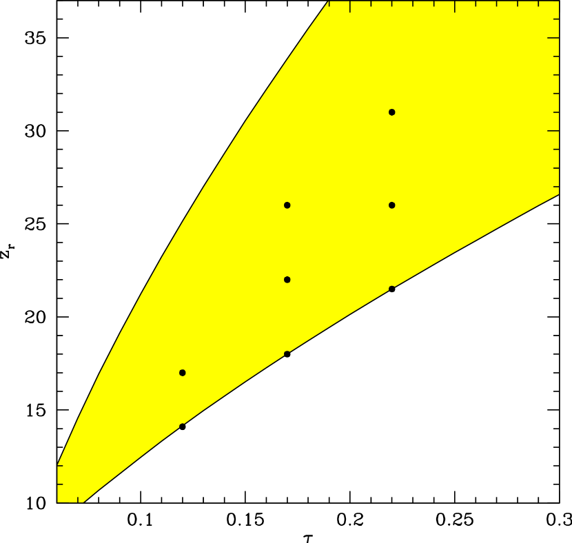
Figure 1: The parameter space allowed in our investigations in the plane $\tau$–vs–$z_{r}$. Dots show the position of fiducial models analyzed in this work. Fiducial models falling on the bottom edge have a single reionization.

Then, the low–ionization period, lasting from a redshift $z_{1}$ to $z_{2}=7$, reduces to zero. For any greater $z_{r}$,

$$\tau\simeq\tau_{2}+{\rho_{b}(z_{2})\over m_{p}}\sigma_{T}ct_{2}\left[\big{(}{1+z_{r}\over 1+z_{2}}\big{)}^{3\over 2}-{2\over 3}\big{(}{1+z_{1}\over 1+z_{2}}\big{)}^{3\over 2}-{1\over 3}\right]$$ (1)

Here $\sigma_{T}$ is the Thomson cross–section, $m_{p}$ is the average baryon mass, $\rho_{b}(z_{2})$ the baryon matter density at redshift $z_{2}$; $t_{2}$ is the time corresponding to $z_{2}$, $\tau_{2}$ is the optical depth due to full reionization since $t_{2}$. In eq. (1) a matter dominated expansion is assumed, since $z_{r}$ to $z_{2}=7$, yielding an error of a few percent. Given $\tau$ and the $(1+z_{r})/(1+z_{2})$ ratio, eq. (1) fixes the ratio $(1+z_{1})/(1+z_{2})$. There is however a top value for $z_{r}$, achieved when $z_{r}=z_{1}$; this sets the upper side of the shaded area in Figure 1 (obtained through exact numerical integration). Then, the first $x_{e}=1$ period, lasting from $z_{r}$ to $z_{1}$, reduces to zero.

A first reionization occurring at a redshift $z_{r}\gg 30$ is unlikely under most models of ionizing sources (see, e.g., Haiman & Holder haho (2003)); therefore, not all points falling within the shaded area of Fig. 1 bear the same physical relevance, in spite of being compatible with the parametrization of reionization discussed here.

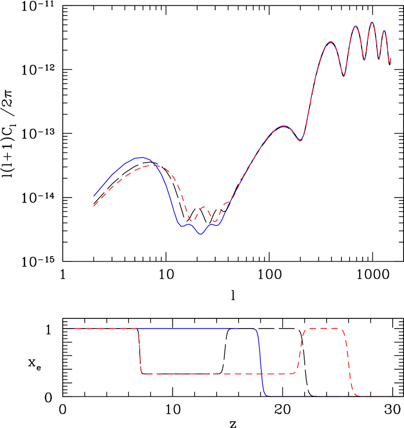
Figure 2: E-mode angular power spectra (top panel) and ionization history (bottom panel) for three different models considered in our analysis with $\tau=0.17$. Solid line represent a ionization profile with $z_{r}=18$, long–dashed line has $z_{r}=22$ and short–dashed line $z_{r}=26$. Different ionization levels are connected by a fast but smooth transition in order to guarantee stability in numerical integration.

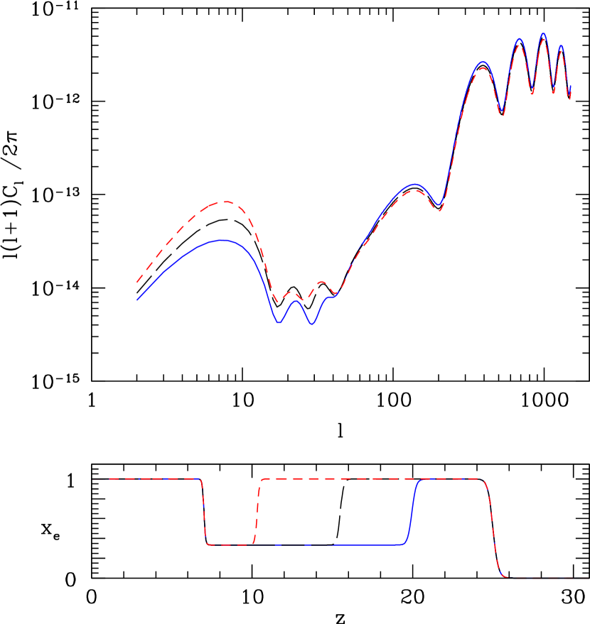
Figure 3: $C_{l}^{E}$ power spectra and ionization histories for three models with $z_{r}=25$ and $\tau=0.17$ (solid line), $\tau=0.21$ (long-dashed line), $\tau=0.25$ (short-dashed line).

When modifying the CMBFAST linear code, we are very careful in treating on ionization transients. Analytical and numerical approximations at each shift are the same as used in CMBFAST when dealing with a single reionization event. In particular, to avoid instabilities in numerical integration, due to fast variations in $x_{e}$, we adopt grid steps $s_{\tau}=.01$ and $s_{z}=1$.

In Figure 2, we show the varying ionization rates and the resulting CMBP $E$–mode spectra for a set of models with equal $\tau$ but different $z_{r}$. Conversely, in Figure 3, we show models where the first reionization redshift $z_{r}$ is kept constant and $\tau$ is variable. The models of Figure 2 lie on a vertical line of Figure 1, those of Figure 3 lie on a horizontal line in the same figure. Power spectra are clearly sensitive to the ionization history and potentially encode information on it. Notice that varying $\tau$ has effects extending to greater $l$, while varying $z_{r}$ produces effects limited to $l\la 50$. In the next sections we discuss how far these variations are detectable at different levels of instrumental sensitivity.

3 Likelihood Analysis

Large angular scales are significantly affected by CV and a given model can yield significantly different skies. To evaluate how far large angle CMB experiments can recover the reionization history, we adopt a Monte Carlo approach.

The basic outline of our approach is as follows. We select a fiducial cosmological model $\tilde{\cal M}$ and generate 5000 sky maps, with resolution and beam smoothing similar to those of actual experiments. To each CMB map we add a noise map; the resulting maps for the anisotropy $T$ and the $Q$, $U$ Stokes parameters are then used for likelihood evaluation. The probability distribution function (p.d.f.) for the parameters characterizing the model $\tilde{\cal M}$ is then simply the distribution of the best–fit parameters in the likelihood analysis of such maps.

In this work we deal with polarization data similar to those expected from the SPOrt experiment, however allowing for a higher sensitivity, while temperature data are supposed to come from an experiment similar to WMAP. Simulated maps are generated using the HEALPix package. Both $T$ and $Q,U$ data are smoothed with a $7\degr$ FWHM Gaussian filter and we chose a HEALPix resolution $N_{side}=16$ (corresponding to a pixel width of $\sim 3.5\degr$). This approach results in a rather low number of pixels, while parameter extraction is sensitive only to $l\la 40$ multipoles. Each simulated map represents a random realization of the process $\tilde{\cal M}+{\cal N}$. The noise model ${\cal N}$ is assumed to be uniform and white, and is then fully defined by the rms noise values $\sigma_{T}$ and $\sigma_{P}$ for $T$ and $Q,\leavevmode\nobreak\ U$ pixels.

As explained in the Introduction, we remove the region with Galactic latitude $|b|<20\degr$ from $T$ maps, where Galactic contamination strongly surpasses the CMB signal. On the other hand, the synchrotron template developed by Bernardi et al. (2004) shows that at 90 GHz the synchrotron polarized emission in the Galactic Plane is at most comparable with the CMB polarization signal for a cosmological model with optical depth $\tau=0.17$. Taking into account that foreground removing techniques allow one to lower the foreground contamination by a significant amount (by a factor $\sim 5$–10), the residual contamination is likely to affect the CMB polarization analysis to a negligible extent, and we choose not to remove the Galactic Plane in the present analysis of ($Q,\leavevmode\nobreak\ U$) maps. Still, part of the Galactic Plane is cut out by excluding declinations $|\delta|>51.6\degr$, which SPOrt is unable to inspect. (In addition, we notice that polarized emission by dust grains is expected to lie safely below synchrotron, at least up to $l\simeq 50$; see Fabbri fabbri (2004) for a more detailed discussion).

Simulated data are ordered into a vector ${\bf x}\equiv\{T(i=1,...,N_{T}),Q(i=1,....,N_{P}),U(i=1,....,N_{P})\}$, $N_{T}$ and $N_{P}$ being respectively the number of anisotropy and polarization pixels. The likelihood of a model ${\cal M}$ is then given by a multivariate Gaussian:

$${\cal L}({\cal M}|{\bf x})={1\over(2\pi)^{N_{T}+2N_{P}}}{1\over\sqrt{\det{\bf C}}}\exp\left(-{1\over 2}{\bf x}^{\rm T}{\bf C}^{-1}{\bf x}\right)\leavevmode\nobreak\ ;$$ (2)

where the correlation matrix reads:

$${\bf C}_{ij}\equiv\langle{\bf x}^{T}_{i}{\bf x}_{j}\rangle={\bf S}_{ij}+{\bf N}_{ij}$$ (3)

(brackets mean ensemble average). Its elements represent the expected correlation between elements of the vector ${\bf x}$. For example, the expected correlation between $T$ signals in the $i$ and $j$ pixels, at an angular distance $\vartheta_{ij}$, reads

$$\langle T_{i}T_{j}\rangle=\sum_{l}{2l+1\over 4\pi}C^{T}_{l}P_{l}(\cos\vartheta_{ij})B^{2}_{l}+(\sigma_{T})^{2}\delta_{ij};$$ (4)

here $C^{T}_{l}$ is the anisotropy spectrum of the model, $P_{l}(\cos\theta)$ are Legendre polynomials, while the coefficients $B^{2}_{l}$ account for pixelization and beam smoothing. For a FWHM of $7\degr$, the correction $B^{2}_{l}$ is relevant even for the lowest harmonics. Similar expressions, taking into account the tensor nature of polarization, hold for correlations involving $Q$ and $U$ data (see, e.g., Zaldarriaga zald98 (1998), Ng & Liu ng (1999)). The effects of sky cuts, here, are directly set by the $i,j$ index domains. This is a clear advantage of working in the coordinate space. (As already outlined, in the harmonic space, $f_{sky}$ corrections are unsafe for large angle experiments or when $T$ and $Q,U$ data cover different portions of the sky.)

For each sky realization, we seek the values of the reionization parameters which maximize the likelihood function $\cal L$. Repeating the operation for a set of realizations allows us to study the resulting distributions.

The fiducial models considered in this work are shown in Figure 1. Each model was tested at 3 levels of sensitivity for the polarization measures: $\sigma_{P}=1.50,\leavevmode\nobreak\ 0.45,\leavevmode\nobreak\ 0.15\,\mu$K for $\sim 7\degr$ pixels, corresponding to $\sim 10,\,3,\,1\,\mu$K–degree. The first value is the expected sensitivity for the 90GHz SPOrt channel. The pixel noise for $T$ data is set at the reference value $\sigma_{T}=1\mu$K. For such $\sigma_{T}$, uncertainties on measurement of $T$–multipoles are dominated by the CV up to $l\approx 500$ while, with our beamwidth and pixelization, only the first $\la 40$-50 multipoles matter. Thus, a $\sigma_{T}$ reduction would not yield a significant gain. On the contrary, as polarization is $\sim 100$ times smaller than anisotropy, sensitivity increases like those considered here improve the ratio between CV and noise variance, mainly in the harmonic range we are exploring. How the different $\sigma_{P}$ values interfere with polarization multipoles must be considered in detail, to understand our results, and will be discussed below.

The distribution of the best fit parameters, among the 5000 CMB realizations of each fiducial model, at the three noise levels, provides a frequentist estimate of the probability density function (p.d.f.) of model parameters. To ensure that CV did not introduce spurious effects in the comparisons of different models, we used the same set of random seeds and of noise maps for all fiducial models. Therefore: (i) Differences between sets of sky maps with the same noise level are due only to changes in the CMB power spectra between the fiducial models. (ii) Differences between sets of maps at different sensitivities (but corresponding to the same model) are only due to variations in the noise.

4 Results

All fiducial models were analyzed first assuming a single reionization, then considering reionization histories of the kind described in Sec. 2. We compare the probability distributions on $\tau$, to test the bias induced by the prior of sharp reionization.

Table 1: Fiducial models: $\tau$ is the total optical depth, $z_{r}$ is the redshift of the first reionization. Models with the superscript $s$ have a sharp reionization history, other models assume that the Universe is completely reionized at $z<7$, while between these two reionization periods $x_{e}$ drops to 1/3.

	${\cal A}^{s}$	$\cal B$	${\cal C}^{s}$	$\cal D$	$\cal E$	${\cal F}^{s}$	$\cal G$	$\cal H$
$\tau$	0.12	0.12	0.17	0.17	0.17	0.22	0.22	0.22
$z_{r}$	14.1	17	18.0	22	26	21.4	26	31

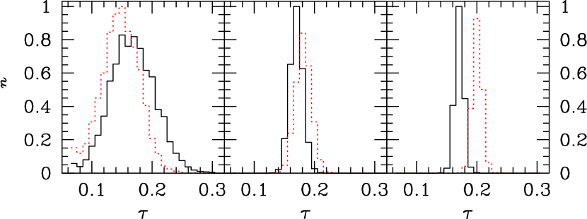
Figure 4: Distribution of $\tau$ for models ${\cal D}$, at different noise sensitivity (left to right, $\sigma_{P}=1.50,\,0.45,\,0.15\,\mu$K). Solid lines show results obtained marginalizing over $z_{r}$, dotted lines refer to results of checking the same realizations against single reionization models. At high sensitivity, the latter prior give rise to a noticeable bias.

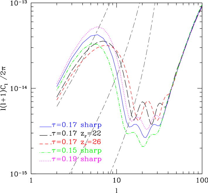
Figure 5: E–mode angular power spectra for models ${\cal C}$ (solid lines), ${\cal D}$ (long–dashed lines), ${\cal E}$ (short–dashed) and two sharp reionization models with $\tau=0.15$, 0.19 (dot–dashed and dotted lines respectively). At given value of the optical depth, spectra of models with double reionization fall below the APS of a sharp reionization with same $\tau$ for $l\leavevmode\nobreak\ {\tilde{<}}\leavevmode\nobreak\ 8$–10 and above for $10\leavevmode\nobreak\ {\tilde{<}}\leavevmode\nobreak\ l\leavevmode\nobreak\ {\tilde{<}}\leavevmode\nobreak\ 40$. The long–short dashed lines, instead, show the noise spectra for different pixel noises on polarization (top to bottom $\sigma_{P}=1.50,\,0.45,\,0.15\,\mu$K), corrected for pixelization and beam smoothing.

In Fig. 4, we compare the $\tau$ distributions obtained under the prior of single reionization (dotted lines) with those obtained after marginalizing over $z_{r}$ the joint distribution on $\tau$ and $z_{r}$ (solid lines). The three plots account for three polarization noise levels. At each level, no significant difference between the width of the two distributions is apparent. However, while all marginalized distributions peak at the true optical depth $\tau=0.17$, the single reionization distributions show a bias, depending on $\sigma_{P}$, similarly to Holder et al. (bias (2003)). Let us however outline a further trend: if $\sigma_{P}=1.50\,\mu$K, the single reionization prior leads to underestimating $\tau$, although within the (still wide) statistical error; as $\sigma_{P}$ decreases, the peak $\tau$–value increases and, at the top sensitivity considered, $\tau$ is overestimated by more than two standard deviations.

This happens because the range of $C^{E}_{l}$ significantly affecting the estimates is strongly related to $\sigma_{P}$, for the sensitivity levels we are considering. In fact, $\tau$ accounts for the number of scattered CMB photons, which can affect the total amount of large scale polarization (Zaldarriaga zald97 (1997)). Therefore, the $E$–spectra, for models with different $\tau$ but equal $z_{r}$, differ mainly in the height of the first reionization peak. But a variation of $z_{r}$ – at fixed $\tau$ – also shifts the peak in $l$. Fig. 5 shows the $E$–spectra for the models ${\cal C,D,E}$, plus two single reionization models, with $\tau=0.15$ and $\tau=0.19$. For models with $\tau=0.17$, when $z_{r}$ increases, the first reionization peak moves to greater $l$ and its height slightly decreases: then $l\la 8$ harmonics of models ${\cal D}$ and ${\cal E}$ approach those for single reionization with lower $\tau$; the same models, in the range $8\la l\la 20$, resemble a single reionization with greater $\tau$.

When $\sigma_{P}=1.50\,\mu$K (top noise level considered), reionization parameters are mostly determined by the first 6–7 multipoles, the only ones clearly above noise (see Fig. 5). Trying to fit a single reionization to a double reionization history therefore leads to underestimating $\tau$. As the noise decreases and multipoles in the range $10\la l\la 20$ acquire a greater weight, a double reionization history can be misinterpreted as single reionization with a greater $\tau$.

The shift of the reionization peak to greater $l$ is typical of models with complex reionization histories. Hence, this low–$\sigma$ high–$\tau$ effect, when a single reionization is assumed, should be independent of reionization details, for the range of sensitivities considered here. For higher sensitivities, when multipoles $20\la l\la 40$ affect the $\tau$ determination, the $E$–spectrum exhibits further peaks, whose details are related to model features, and the trend will depend on the set of models considered.

In general, the bias is stronger for greater $\tau$ and, at fixed $\tau$, it increases with $z_{r}$. At noise levels accessible to current experiments’ statistical errors exceed the bias, and $\tau$ estimates are safe, although systematically smaller than the real values. In higher sensitivity experiments, wrong priors can cause a $\tau$ overestimate, exceeding several standard deviations. An opposite behavior is found when single reionization models are analyzed assuming a two–reionization history. In this case, however, the bias is not so severe.

The low–$\sigma$ high–$\tau$ effect can be used to test the reionization pattern, by comparing early and late outputs, in a long lived experiment. Detecting a clear trend requires a sensitivity increase by at least a factor $\ga 3$. As we are considering low multipoles, early outputs must cover the whole sky with a reasonable sensitivity. Assuming that a full sky coverage requires $\sim 6$ months, the total experimental lifetime should be $\sim 5$–6 years. The required increase is unlikely within the planned lifetime of current experiments, but could be an option for future polarization missions.

We performed some more detailed tests of this point. (i) For each realization we labeled $\tau^{s}_{1.50},\,\tau^{s}_{0.45}\,\tau^{s}_{0.15}$ ($\tau^{d}_{1.50},\,\tau^{d}_{0.45}\,\tau^{d}_{0.15}$) the optical depth estimated at $\sigma_{P}=1.5,\leavevmode\nobreak\ 0.45,\leavevmode\nobreak\ 0.15\,\mu$K, under a single (double) reionization prior. (ii) We selected the realizations where the $\tau$ estimates, under a single reionization prior, increased at both noise reductions ($\tau^{s}_{1.50}<\tau^{s}_{0.45}<\tau^{s}_{0.15}$). (iii) Among them we kept those for which the shift $\tau^{s}_{0.15}-\tau^{s}_{1.50}$ exceeded twice $\tau^{d}_{0.45}-\tau^{d}_{1.50}$. This residual fraction averages $\sim 65\%$; although varying from $\sim 20\%$ (model ${\cal B}$) to more than $90\%$ (model ${\cal H}$). A progressive shift to higher values in single–reionization $\tau$ estimates, when sensitivity increases, therefore can be considered as a hint that a more refined description of reionization is needed.

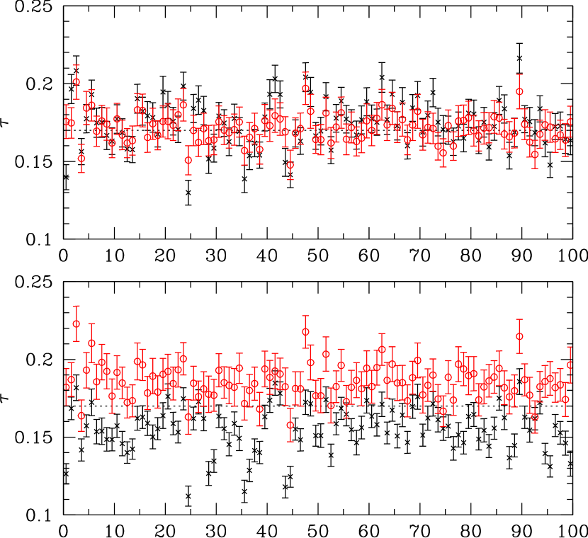
Figure 6: Top. Open circles: $\tau$ from a WMAP+SPOrt–like experiment, with $\sigma_{P}=0.40\mu$K in 5 years, for 100 realizations of model ${\cal D}$, and with a fair double reionization prior. Crosses: average $\tau$ obtained by dividing the whole data set into 10 subsets (6 months observation time). Error bars yield the 1–$\sigma$ c.l. Bottom. The same as Top panel but assuming a sharp reionization prior. Global (averaged) estimates are shifted up(down)–ward in respect to the actual $\tau$ value.

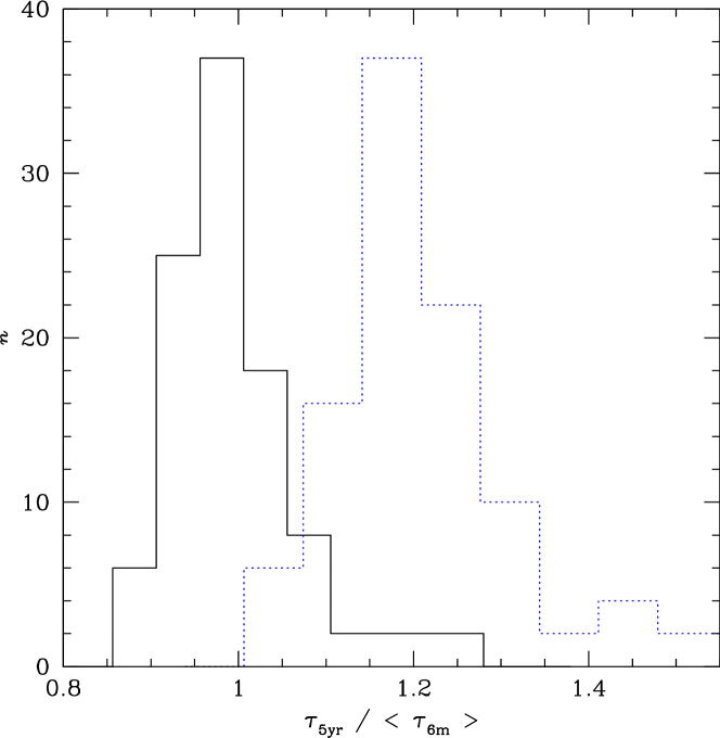
Figure 7: Distribution of the ratio between global and averaged $\tau$ estimates in 100 realizations of model ${\cal D}$, assuming either double realizations (solid line) or sharp reionization (dotted line) priors.

An additional test, for long lived experiments, is provided by dividing the global dataset into subsets corresponding to shorter observation periods, and comparing the $\tau$ value estimated by the analysis of the full dataset with the weighted average of the estimates in the smaller subsets. For reference purposes, we considered a SPOrt–like experiment lasting 5 years, and achieving a polarization pixel sensitivity $\sigma_{P}=0.40\mu$K ($N_{side}=16$). Neglecting correlated noise effects and assuming that a full sky coverage requires 6 months of observations, the global data can be divided into 10 smaller subsets, characterized by $\sigma_{P}\sim 1.25\mu$K. We then compared the global $\tau$ estimate with the average of the estimates in the smaller subsets. Repeating this analysis for 100 random realizations of model $\cal D$, we found global and averaged estimates to be consistent with each other and with the actual $\tau$, when correct priors are made (top panel in Fig. 6). On the contrary, when sharp reionization is assumed, averaged estimates are systematically lower than the correct value, while global measurements overestimate it (bottom panel in Fig. 6). Then, in Fig. 7, we plot the distribution of the ratio between the full 5–year estimate and the averaged 6–month estimates. Assuming a correct prior, such ratio averages $\tau_{5yr}/\langle\tau_{6m}\rangle\,=0.99\pm 0.07$, while for sharp reionization $\tau_{5yr}/\langle\tau_{6m}\rangle\,=1.20\pm 0.10$.

We now adopt a double reionization prior, and discuss the precision by which $\tau$ and $z_{r}$ can be recovered. Marginalizing the joint probability distribution in the $\tau-z_{r}$ plane on either parameter provides the 1D probability density for the other parameter. The variances of these distributions, averaged over fiducial models, tell us how far the models can be discriminated at each sensitivity; results are displayed in Table 2: two equal–$\tau$ models can be distinguished if their $z_{r}$ are farther apart than $\sim$twice the value shown. These uncertainties are close to those obtained in the analysis of the performance of high resolution experiments with equivalent sensitivities (see, e.g., Kaplinghat et al. kap (2003)). Thus, low angular resolution is not a serious impediment in reionization studies.

Table 2: Average statistical errors for the recovered parameters as a function of polarization sensitivity $\sigma_{P}\,(\mu$K).

$\sigma_{P}$	$\Delta_{\tau}$	$\Delta_{z_{r}}$
1.50	0.037	5.0
0.45	0.012	2.6
0.15	0.008	1.4

Within the allowed region of parameter space (see Fig. 1 and discussion), Table 2 implies that $\tau$ is better fixed than $z_{r}$, if the priors on the reionization history are correct. This confirms that also for double reionization, optical depth is the most relevant parameter. At a fixed noise level, models with higher $\tau$ generally allow for a better estimation of both parameters, due to their higher signal-to-noise (S/N) ratio; among models with the same optical depth those with lower $z_{r}$ have slightly sharper redshift distributions, because for very early first reionization, the differences between spectra with distinct $z_{r}$ are less pronounced.

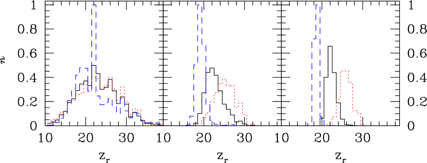
Figure 8: Distribution of maximum likelihood $z_{r}$, after marginalizing over $\tau$, for 5000 realizations of models ${\cal C}$ (dashed lines), ${\cal D}$ (solid lines) and ${\cal E}$ (dotted lines). From left to right, panels refer to $\sigma_{P}=1.50,\,0.45,\,0.15\,\mu$K, respectively.

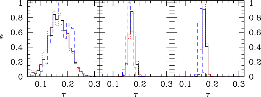
Figure 9: Same as Fig. 8, but for $\tau$ after marginalization over $z_{r}$.

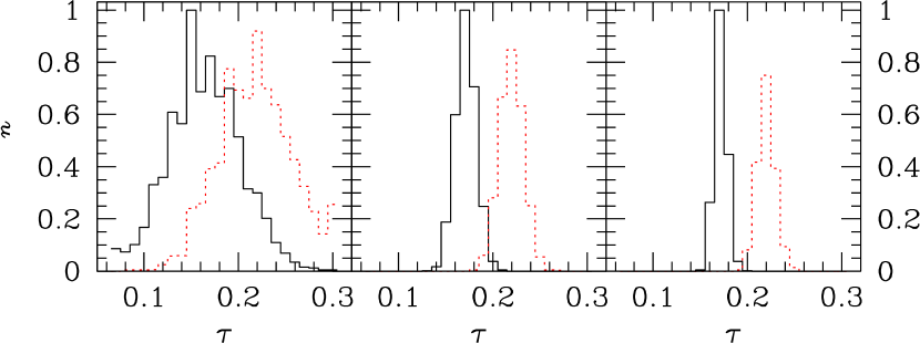
Figure 10: Same as Fig. 9, but for models ${\cal E}$ (solid lines) and ${\cal G}$ (dotted lines).

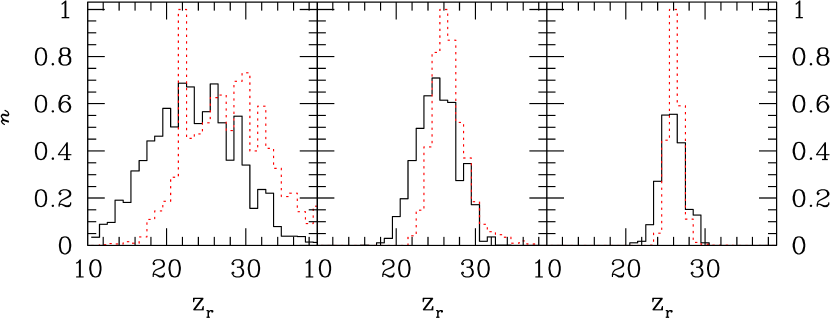
Figure 11: Same as Fig. 10, but for $z_{r}$.

In more detail, Fig. 8 shows the distribution of $z_{r}$ for models with $\tau=0.17$ (see caption for details). For $\sigma_{P}=1.50\mu$K (left panel), the probability distributions overlap significantly, and $z_{r}$ cannot be recovered, while for $\sigma_{P}=0.15\mu$K (right panel) they are almost completely distinguished. The middle panel displays an intermediate situation where models with single reionization can be distinguished from double reionization models with $z_{r}$ in the upper half of the allowed range (i.e. $z_{r}\ga 25$ for $\tau=0.17$). Moreover, distributions on $z_{r}$, in double reionization models, are wider by a factor $\sim 2$ than in single reionization models. Figure 9 shows that the probability distributions on $\tau$, in models ${\cal D}$ and ${\cal E}$, are indistinguishable at all sensitivities; thus, differences in $z_{r}$ do not greatly affect the ability to recover $\tau$, if correct priors are used. Model ${\cal C}$, instead, displays a bias, as discussed above. In this case, $\tau$ is progressively underestimated for decreasing $\sigma_{P}$, as a single reionization model is analyzed assuming a double reionization prior.

In Fig. 10 we plot the distributions on $\tau$ for models with equal $z_{r}$ but different $\tau$ (${\cal E}$ and ${\cal G}$). Even at the highest noise, a difference can be seen; for $\sigma_{P}=0.45\,\mu$K the two distributions are clearly separated. In both cases, the correct $\tau$ is recovered. Figure 11, instead, shows results for $z_{r}$. The probability distributions of both models exhibit a significant overlap and correctly peak at the true value of the reionization redshift. Model ${\cal G}$, however, is characterized by a sharper and better defined distribution, due to its higher S/N ratio.

We can summarize our findings as follows. (i) Constraints on the reionization history from large–angle experiments are similar to those by high–resolution experiments with equivalent sensitivity. For instance, a polarization noise $\sigma_{P}=1.50\,\mu$K allows one to constrain the total optical depth with an accuracy of $\sim 20\%$ for $\tau=0.17$. Increasing sensitivity by an order of magnitude allows for a simultaneous detection of $\tau$ and $z_{r}$, with an accuracy $\la 5\%$. (ii) A wrong prior on the reionization history causes a bias in the $\tau$ estimate. For $\sigma_{P}=1.50\,\mu$K the statistical uncertainty exceeds the bias, while for $\sigma_{P}=0.15\,\mu$K the bias may exceed 3 standard deviations. This point, too, agrees with previous works studying the capabilities of high resolution CMB polarization measurements. Thus high resolution, by itself, does not provide more reliable estimates. (iii) At current noise levels, $\tau$ is underestimated, while, for increasing sensitivities, it tends to be overestimated. This is likely due to the first reionization peak moving to higher $l$’s in models with complex reionization, with respect to sharp reionization models with the same $\tau$.

(iv) Finally, we suggest an observational approach to discriminate between single and double reionization histories, based on such low–$\sigma$ high–$\tau$ effect. For illustration, we considered a mission lasting $5\,$years, allowing a pixel sensitivity $\sigma_{P}\sim 0.4\,\mu$K. We assumed that full sky coverage requires 6 months so that the full dataset can be divided into 10 smaller subsets, with a sensitivity worse by a factor $\sim 3$. Assuming no systematic effects, the 10 subsets provide as many independent $\tau$ estimates. When the correct priors on reionization are assumed, the global estimate is consistent with the average of the estimates from the smaller subsets; on the contrary, assuming a sharp reionization prior, the 5–year $\tau$ value systematically exceeds both the correct value and the average of the 6–month estimates. Accordingly, in future low–noise experiments, it can be significant to compare whole–run $\tau$ estimates, with full sensitivity, with averages among short run estimates. Similar error bars are expected, but a shift of the estimated $\tau$ would indicate that the assumed reionization pattern could be a source of bias.

5 Conclusions

In this work we discussed a class of physically motivated double reionization models, characterized by two parameters: the total optical depth $\tau$, and the first reionization redshift $z_{r}$. We determined at which sensitivity level their features can be recovered by large angle CMBP measurements. We find that wrong priors on the history of reionization can lead to a bias in $\tau$ estimates, in agreement with findings for high resolution experiments (Holder et al. bias (2003)). At the WMAP or SPOrt noise level, the bias is well within statistical errors; at higher sensitivities the $\tau$ estimate can lie several standard deviations from its true value. Holder et al. (bias (2003)) argue that fitting a two–step reionization to the models they considered allows one to significantly reduce the bias. In addition we find that, for the class of models considered here, the biased $\tau$ estimates exhibit a characteristic dependence on experimental sensitivity. Testing this low–$\sigma$ high–$\tau$ effect in actual experiments provides an indication of the fairness of priors.

Within the context of double reionization models, a pixel noise $\sigma_{P}=1.50\,\mu$K for $7\degr$ pixels, allows one to constrain $\tau$ with an accuracy $\sim 20\%$; an increase in sensitivity by a factor $\sim 3$ enables us to distinguish single reionization models from models with an early reionization (i.e. $z_{r}\ga 25$ for $\tau=0.17$) followed by a partial recombination period. Models of ionizing sources rarely yield $z_{r}\ga 30$. Firm measurements of both $\tau$ and $z_{r}$, with precisions $\sim 5\%$, require a sensitivity increase by an order of magnitude. Greater spatial resolution, instead, is not very relevant, as most information on reionization is carried by the first 30–40 multipoles of the $E$–spectrum.

Measures of $C_{l}^{E}$ at large angular scales are an important probe of the evolution of ionizing sources at redshifts $10\la z\la 30$. However, as finer data become available, the situation becomes more and more risky. Unless an accurate class of models is fitted to data, parameter misestimates can occur: apparent errors can seem small, while true values lie well off the 3 $\sigma$ error interval. A test of the reliability of the overall $\tau$ estimate can be however performed by comparing estimates from the whole data set with those from smaller representative subsets. A clear detection of this low–$\sigma$ high–$\tau$ effect requires an increase in sensitivity by a factor $\sim 3$. Assuming that full sky coverage requires 6 months, the effect can be evident in experiments lasting $\sim 5$–6 years.

- (1) Becker, R.H., Fan, X., White, R.L., et al., 2001, AJ, 122, 2850
- (2) Bennett, C.L., Hill, R.S., Hinshaw, G., et al., 2003 ApJS, 148, 97
- (3) Bernardi, G., Carretti, E., Fabbri, R., et al. 2004 MNRAS, 351, 436
- (4) Bruscoli, M., Ferrara, A., & Scannapieco, E. 2002 MNRAS, 330, L43
- (5) Cen, R. 2003, ApJ, 591, 12
- (6) Ciardi, B., Ferrara, A., & White, S.D.M., 2003, MNRAS, 344, L7
- (7) Colombo, L.P.L. 2004, JCAP, 3, 3
- (8) Cortiglioni, S., Bernardi, G., Carretti, E., et al. 2004, New A, 9, 297
- (9) Djorgovski, S.G., Castro, S., Sterm, D., & Mahabal, A.A. 2001, ApJ, 560, L5
- (10) Fabbri, R. 2004, in Proceedings of the 2004 SAIT meeting ’ 48-esimo Congresso della Societ Astronomica Italiana: I Colori dell’Universo - Astronomia Italiana dalla Terra e dallo Spazio’ eds. Wolter, A., Isreal, G. & Bacciotti, F. 2004, in press
- (11) Haiman, Z., & Holder, G.P. 2003, ApJ, 595, 1
- (12) Hansen, S.H. & Haiman, Z. 2004, ApJ, 600, 24
- (13) Holder, G.P., Haiman, Z., Kaplinghat, M., & Knox, L. 2003, ApJ, 595, 13
- (14) Hu, W., & Holder, G.P. 2003, Phys. Rev. D, 68, 3001
- (15) Kaplinghat, M., Chu, M., Haiman, Z., et al. 2003, ApJ, 583, 24
- (16) Kogut, A., Spergel, D.N., Barnes, C., et al. 2003, ApJS, 148, 161
- (17) Madau, P., Rees, M.J., Volonteri, M., Haardt, F., & Oh, S.P. 2004, ApJ, 604, 484
- (18) Malhotra, S., & Rhoads, J. 2004, ApJ, submitted, astro-ph/0407408
- (19) Miralda–Escudè, J. 2003, ApJ, 596, 66
- (20) Naselsky, P., & Chiang, L.Y. 2004, MNRAS, 347, 975
- (21) Ng, K.–W. & Liu, G.–C. 1999, Int. J. Mod. Phys. D8, 61
- (22) Ricotti, M., & Ostriker, J.P. 2004, MNRAS, 350, 539
- (23) Ricotti, M., & Ostriker, J.P. 2004, MNRAS, 352, 547
- (24) Seljak, U., & Zaldarriaga, M, 1996, ApJS, 469, 473
- (25) Sokasian, A., Yoshida, N., Abel, T., Hernquist, L., & Springel, V. 2004, MNRAS, 350, 47
- (26) Wyithe, J., Stuart, B., & Loeb, A. 2003, ApJ, 586, 693
- (27) Zaldarriaga, M. 1997, Phys. Rev. D, 55, 1822
- (28) Zaldarriaga, M. 1998, ApJ, 503, 1