Evolving dark energy equation of state and CMB/LSS cross-correlation

Abstract

CMB power spectra and the SNIa luminosity-redshift curves have difficulty distinguishing between models with the same average value of the dark energy equation of state. We propose using the cross-correlation of the CMB temperature anisotropy with large scale structure to help break this degeneracy.

The evidence for Dark Energy (DE), a dark component causing the accelerated expansion of the universe, comes from several complementary sources. The analysis of the cosmic microwave background (CMB) shows that the total energy density of the universe is very close to the critical density, i.e. the universe it flat. At the same time, large scale structure (LSS) measurements suggest that no more than a third of the critical energy density can be in the form of clustering matter. While CMB and LSS measurements, if considered separately, can be explained without invoking DE, they require DE for consistency with each other. wmap_spergel ; tegmark_etal . A more direct evidence for DE comes from measurements of the luminosity distance vs redshift for supernovae type Ia (SNIa) Riess ; Perlmutter revealing an accelerated expansion of the universe. For a flat Freedman-Robertson-Walker (FRW) universe acceleration implies domination by a substance with negative pressure, such as vacuum energy. Another direct evidence which has recently become available is the detection of the Integrated Sachs-Wolfe (ISW) effect using the CMB/LSS cross-correlation xray ; nolta ; fosalba ; scranton ; afshordi03 ; vielva04 ; padma04 . This evidence is of complementary nature to the SNIa data. Rather than probing the accelerated expansion it reflects the slow down in the growth of density perturbations expected in a non-matter dominated universe.

The cosmological constant $\Lambda$ is the simplest DE model giving a satisfactory fit to the existing data. Observations are also consistent with an evolving dark energy, such as the scalar field Quintessence wetterich ; peebles ; caldwell98 . Establishing whether the dark energy is constant or evolving is one of the main challenges for modern cosmology. In the FRW universe the large scale evolution of DE is determined by its equation of state defined as the ratio of pressure to energy density: $w\equiv p/\rho$. For scalar field Quintessence $w$ also determines the clustering properties of DE. Depending on the model $w$ can be constant or change with time. Models with $w\neq-1$ correspond to evolving DE, while $w=-1$ corresponds to $\Lambda$.

Much work has been done on trying to constrain the change in $w$ by fitting various forms of $w(z)$ to the SNIa luminosity distance-redshift data, often in combination with constraints from the CMB power spectrum. It is known, however, that these observables depend on $w(z)$ via one or more integrals over the redshift huey99 ; maor01 ; maor_prd ; dave02 ; ng ; saini03 . As we illustrate below, the CMB power spectra and the luminosity distance curves for models with varying $w(z)$ can be difficult to distinguish from predictions of the model with a constant $w$ equal to the average of $w(z)$ defined as

$$<w>\equiv{\int_{a_{*}}^{1}da\ w(a)\ \Omega_{D}(a)\over\int_{a_{*}}^{1}da\ \Omega_{D}(a)}\ ,$$ (1)

where $a$ is the scale factor, $a=1$ today, $a_{*}$ is the scale factor at the last scattering and $\Omega_{D}(a)$ is the ratio of the DE energy density to the critical density.

The LSS measurements probe the net growth of cosmic structures. Provided other parameters are known, LSS can differentiate between a constant and a time-varying $w$, especially if one had the information about the growth factor at different redshifts linder03 .

Measurements of the ISW effect can provide another probe of the evolution of $w(z)$. In a way, they are more sensitive to the change in $w(z)$ because ISW depends on the growth rate of cosmic structures (the time-derivative of the growth factor) in addition to the total growth (see CHB03 for a useful discussion). In this letter we build on the methods and results of GPV04 and illustrate the potential of the CMB/LSS cross-correlation for constraining the change in $w(z)$. For this purpose we will consider four Quintessence models with the same average $<w>$ shown in Fig. 1. These four models are deliberately chosen to illustrate a point and do not necessarily represent particularly well-motivated quintessence potentials. The ansatz for $w(z)$ used to construct our models is:

$$w(z)=\left[{w_{+}+w_{-}\over 2}\right]+\left[{w_{+}-w_{-}\over 2}\right]\ {\rm tanh}([z-z_{0}]/\delta z)\ .$$ (2)

It is similar in spirit to that of copeland03 and describes a transition from $w_{+}\equiv w(z=+\infty)$ to $w_{-}\equiv w(z=-\infty)$ with parameters $\delta z$ and $z_{0}$ describing the width and the central redshift of the transition. The values of the ansatz parameters used for the four models in Fig. 1 are given in Table 1. The shapes of the corresponding Quintessence potentials can be reconstructed from $w(z)$, if it was desired. These four models have one thing in common – they all have the same $<w>=-0.8$, as defined in eq. (1). This value, $<w>=-0.8$, corresponds to the upper boundary of the $95\%$ confidence region obtained from the combined analysis of the WMAP, SDSS and SNIa data (Fig. 13 of tegmark_etal ).

Model / line type	$w_{-}$	$w_{+}$	$z_{0}$	$\delta z$
$w=-0.8$, solid	-0.8	-0.8	*	*
dot	-0.3	-1	0.15	0.22
short dash	-1	-0.58	0.39	0.09
long dash	-0.4	-1	-0.1	1.55
dot-dash	-1	-0.5	1.	1.98

Table 1: Models considered in the paper.

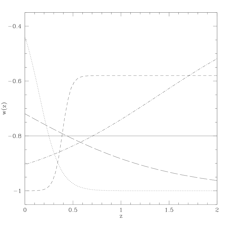
Figure 1: $w$ vs $z$ for the four varying $w(z)$ models considered in this paper. They all have the same average value $<w>$ (solid line) given by eq. 1.

In Fig. 2 we show the CMB spectra for the models in Table 1. The cosmological parameters are the same for all models. Through the paper we assume a flat universe with the Hubble parameter $h=0.66$, baryon density $\Omega_{b}h^{2}=0.024$, total matter density $\Omega_{M}h^{2}=0.14$, spectral index $n_{s}=0.99$, optical depth $\tau=0.166$ and the amplitude of scalar fluctuations $A_{s}=0.86$ (as defined in wmap_verde .) As evident from Fig. 2, all four varying $w$ models fit the WMAP data very well and are indistinguishable from each other and from the model with a constant $w=-0.8$. This agrees with other studies (e. g.  corasaniti03 ) and supports the point made in (among other papers) dave02 that CMB spectra are mainly sensitive to the averaged value of $w$, as defined in eq. (1) .

Figure 2: CMB temperature angular power spectrum (TT) and the temperature-polarization cross-correlation (TE) for the five models in Fig. 1 (using the same conventions for the different line types) with the WMAP’s first year data.

Figure 3: The percent difference in $d_{L}(z)$ for the five models in Fig. 1 and the $\Lambda$CDM model (thick solid line).

The degeneracy between the models persists to a large extent in the luminosity-redshift curves. The SNIa measurements probe the luminosity distance $H_{0}d_{L}(z)$, where

$$d_{L}(z)=(1+z)\int_{0}^{z}{dz^{\prime}\over H(z^{\prime})}\ ,$$ (3)

$H(z)$ is the Hubble parameter and $H_{0}$ is its current value. In Fig. 3 we plot the percent difference between each of the models with varying $w$ and the model of constant $w=-0.8$. As can be seen from the figure, the differences from the $w=const$ case do not exceed $5\%$, which is just about, if not slightly below, the current level of accuracy with which $d_{L}(z)$ is extracted from SNIa. Therefore, a significantly varying $w(z)$ can be consistent with SNIa if the model has a reasonable average $<w>$. Most optimistically, future SNIa data can improve the accuracy in determination of $d_{L}(z)$ to the level of $1-2\%$ maor_prd . As the solid, dash-dot and long dash lines in Fig. 3 show, the future SNIa data may be able to distinguish between an increasing and a decreasing $w(z)$, but there is still likely to be a constant $w$ that gives a very similar $d_{L}$ for the same cosmological parameters. This point was previously emphasized in maor01 ; maor_prd . Fig. 3 also shows a clear difference in predictions of the $w=-0.8$ model and the $\Lambda$CDM model. The $\Lambda$CDM model requires $h=0.72$ for the same $\Omega_{M}h^{2}$ in order to fit the CMB power spectra, hence the $\Lambda$CDM curve in Fig. 3 corresponds to a smaller $\Omega_{M}$.

Figure 4: The linear matter power spectrum for the five models in Fig. 4. The SDSS data points sdss_pk are plotted to show current experimental error bars.

Fig. 4 shows the matter power spectra for the models considered in the paper. Plotted are the linear CDM spectra at $z=0$. A proper accounting for the non-linear effects as well as for the redshift space distortion introduces non-negligible modifications to the amplitudes and the shapes of the spectra. We did not attempt to do that here, assuming that changes in the differences between the curves would be small. The SDSS data points are only plotted to show the uncertainty in the current determination of P(k). Not surprisingly, the models in which $w$ decreases with time are easier to distinguish, because the dark energy component becomes significant and starts to affect the growth of fluctuations early. On the other hand, in models with increasing $w(z)$ the growth of fluctuations is not significantly affected until very recently and the change in $w$ with time is harder to detect. Knowing the matter power spectrum at different redshifts could provide a useful handle on the time-variation of $w$ linder03 .

If one assumes a flat universe with adiabatic initial conditions then the combination of the CMB with SNIa data provides the information about the cosmological parameters and $<w>$. The LSS data tightens the range of parameter values, fixes the galaxy bias and can give some information about the time variation of $w$. Measurements of the CMB/LSS cross-correlation can play a complementary role and provide further constraints on the time variation of $w$. What makes the cross-correlation interesting for this purpose is that it depends not only on the total growth of cosmic structure but on the growth rate as well.

Cross-correlating the CMB with LSS with the purpose of detecting the ISW effect was first proposed in turok96 . Let us define

$$\Delta(\hat{\bf n})\equiv T(\hat{\bf n})-\bar{T}$$ (4)

and

$$\delta(\hat{\bf n})\equiv{\rho(\hat{\bf n})-{\bar{\rho}}\over{\bar{\rho}}}\ ,$$ (5)

where $T(\hat{\bf n})$ is the CMB temperature measured along the direction $\hat{\bf n}$, $\rho(\hat{\bf n})$ is the mass density along $\hat{\bf n}$, and $\bar{T}$ and $\bar{\rho}$ are the averaged CMB temperature and the matter density. The temperature anisotropy due to the ISW effect is an integral over the conformal time:

$${\Delta(\hat{\bf n})\over\bar{T}}=\int_{\eta_{r}}^{\eta_{0}}d\eta(\dot{\Phi}-\dot{\Psi})\left[(\eta_{0}-\eta)\hat{\bf n},\eta\right],$$ (6)

where $\eta_{r}$ is some initial time deep in the radiation era, $\eta_{0}$ is the time today, $\Phi$ and $\Psi$ are the Newtonian gauge gravitational potentials, and the dot denotes differentiation with respect to $\eta$. The quantity $\delta(\hat{\bf n})$ contains contributions from astrophysical objects (e. g. galaxies) at different redshifts and can also be expressed as an integral over the conformal time:

$$\delta(\hat{\bf n})=\int_{\eta_{r}}^{\eta_{0}}d\eta\ {dz\over d\eta}\ W_{g}(z(\eta))\ {\delta}((\eta_{0}-\eta)\hat{\bf n},\eta),$$ (7)

where $W_{g}(z)$ is a normalized galaxy selection function. We do not explicitly include a possible bias factor, assuming it is determined from the measurements of the LSS. We are interested in calculating the cross-correlation function

$$X(\theta)\equiv X(|\hat{\bf n}_{1}-\hat{\bf n}_{2}|)\equiv\langle\Delta(\hat{\bf n}_{1})\delta(\hat{\bf n}_{2})\rangle\ ,$$ (8)

where the angular brackets denote ensemble averaging and $\theta$ is the angle between directions $\hat{\bf n}_{1}$ and $\hat{\bf n}_{2}$. It can be written as GPV04

$$X(\theta) = {9\over 25}\int_{\eta_{r}}^{\eta_{0}}d\eta_{1}\int_{\eta_{r}}^{\eta_{0}}d\eta_{2}\ \dot{z}(\eta_{2})\ W_{g}(z(\eta_{2}))$$

$$\times \int{dk\over k}\Delta_{\cal R}^{2}(k)\ {{\rm sin}(kR)\over kR}\ F(k,\eta_{1},\eta_{2})\ ,$$

where $k$ is the wave-number, $\Delta_{\cal R}^{2}(k)$ is the primordial curvature power spectrum, $F(k,\eta_{1},\eta_{2})$ describes the time-evolution of $(\dot{\Phi}-\dot{\Psi})$ and $\delta$, $R\equiv\sqrt{r_{1}^{2}+r_{2}^{2}-2r_{1}r_{2}{\rm cos}\theta}$ and $r\equiv\eta_{0}-\eta$ (see GPV04 for more details) .

The galaxy window function $W_{g}(z)$ plays an important role as it essentially zooms in on the ISW effect over a particular redshift range. To help one decide on the selection of $W_{g}(z)$ it is useful to define $I(\theta,z)$ as

$$I(\theta,z)\equiv{9\over 25}\int_{\eta_{r}}^{\eta_{0}}d\eta_{1}\int{dk\over k}\Delta_{\cal R}^{2}(k)\ {{\rm sin}(kR)\over kR}\ F(k,\eta_{1},\eta_{2})\ ,$$ (10)

so that eq. (LABEL:wtg3) can be written as

$$X(\theta) = \int_{z_{r}}^{0}dz\ W_{g}(z)I(z,\theta)\ .$$ (11)

Typically, the theoretical prediction for the cross-correlation approaches a flat plateau for $\theta<0.2^{\circ}$ and the hight of the plateau is a good measure of the overall signal. In Fig. 5 we plot $I(z,\theta=0.2^{\circ})$ vs $z$ for the models considered in the paper. From this plot one can guess where to place the window function to see the maximum difference in $X(\theta)$ for the models. This, however, may not correspond to the choice that gives the highest signal-to-noise ratio. Due to the arbitrary nature of the models considered in the paper we did not search for the optimal window function(s) that would maximize the difference between the models while minimizing the statistical uncertainty in $X(\theta)$. Such optimization procedure, however, would be necessary if the cross-correlation was used to study properties of dark energy.

Figure 5: The integrand $I(z,\theta=0.2^{\circ})$ for the five models in Fig. 4. Plotted on top (long dash-dot) are the two choices of window functions used in the paper, rescaled to fit the box.

For computational purposes it is advantageous to decompose $X(\theta)$ into a Legendre series,

$$X(\theta)=\sum_{l=2}^{\infty}{2\ell+1\over 4\pi}X_{\ell}P_{\ell}({\rm cos}\ \theta)\ .$$ (12)

In Fig. 6 we show results for the angular cross-correlation $l(l+1)X_{\ell}/2\pi$ for the two choices of Gaussian window functions shown in Fig. 5. One is centered at $z_{w}=0.3$ and the other at $z_{w}=0.6$, both have a standard deviations of $\Delta z=0.15$. The two window functions are chosen so that the first one results in the larger difference between the models, while the second one gives the larger signal-to-noise ratio. Theoretical uncertainties in individual $X_{\ell}$ are too large to allow comparing the models at each $\ell$.

Figure 6: The angular cross-correlation, $l(l+1)X_{l}/2\pi$ for the five models in Fig. 4 and two choices of window functions. Theoretical uncertainties in individual $X_{\ell}$, if plotted, would be well outside the boundaries of the box. Instead, we propose using the cumulative cross-correlation (summed over $\ell$) to differentiate between the models.

Instead one could calculate the total signal, $X_{T}$, for each model by summing $(2l+1)X_{\ell}/4\pi$ over $\ell$:

$$X_{T}=\sum_{\ell=2}^{\ell_{\rm max}}{2\ell+1\over 4\pi}X_{\ell}\ .$$ (13)

Note that, for $l_{\rm max}=\infty$, $X_{T}=X(\theta=0)$. The best achievable signal-to-noise in determination of $X_{T}$ is approximately given by

$$\left({S\over N}\right)^{2}\approx f_{\rm sky}\sum_{\ell=2}^{\ell_{\rm max}}(2\ell+1){X_{\ell}^{2}\over C_{\ell}^{TT}C_{\ell}^{MM}}\ ,$$ (14)

where $f_{\rm sky}$ is the surveyed fraction of the sky, $C_{\ell}^{TT}$ is the angular CMB temperature power spectrum and $C_{\ell}^{MM}$ is the analogously defined matter angular spectrum inside a given window $W_{g}(z)$. Table 2 contains $X_{T}$ for each model for the two choices of the window functions.

Model/line type	$X_{T}(z_{w}=0.3)$	$X_{T}(z_{w}=0.6)$
$w=-0.8$, thick solid	0.167	0.125
dot	0.187	0.137
short dash	0.132	0.108
long dash	0.175	0.132
dot-dash	0.144	0.106

Table 2: The cumulative cross-correlation $X_{T}$, in $\mu K$, for $\ell_{\rm max}=300$ for the models considered in the paper and the two choices of window functions.

The table shows differences of up to $\sim 35\%$ in $X_{T}$ for the window function centered at $z_{w}=0.3$ and up to $\sim 25\%$ for the one centered at $z_{w}=0.6$. The signal-to-noise does not significantly depend on the particular model. Typically, $S/N\approx 2$ for the window function with $z_{w}=0.3$ and $S/N\approx 3$ for $z_{w}=0.6$, assuming complete sky coverage ($f_{\rm sky}=1$) and that $C_{\ell}^{TT}$ contains not just the ISW contribution but the entire CMB anisotropy on relevant scales. Neither choice of the window function would distinguish between the models considered in the paper. There is hope, however, that the uncertainty in $X_{T}$ can be reduced to the level that would allow model comparison.

The potential accuracy that can be achieved in cross-correlation measurements was studied in cooray ; afshordi04 ; scranton04 . The main theoretical uncertainty arises from limitations imposed by cosmic variance and the fact that, in addition to the ISW contribution, the CMB signal has a sizable primary component. A possible way to increase the signal to noise, proposed in afshordi04 , is to consider the cross-correlation in multiple redshift shells. If the shells could be selected in a way that they were nearly uncorrelated then one could treat the cross-correlation in each shell as a separate measurement. Based on the results of afshordi04 it appears that the best accuracy one could hope for is about $10\%$. If this was the case, the cross-correlation could be useful for adding to the constraints on rapidly varying $w(z)$. The CMB/LSS correlation could also help with constraining the clustering properties of Dark Energy (see e.g. scranton04 ; ps05 ).

There is still room for a better understanding of the inherent limitations of the cross-correlation analysis. In particular, there is need for a procedure that would optimize the selection of redshift shells to maximize the signal to noise. This, as well as the constraints from the existing data on the variation of $w(z)$, is a subject of ongoing work RobBobP .

- (1) D. Spergel et al (WMAP collaboration), Astrophys. J. Suppl. 148, 175 (2003).
- (2) M. Tegmark et al (SDSS collaboration), Phys. Rev. D69 103501 (2004).
- (3) A. Riess et al, Astron. J. 116, 1009 (1998).
- (4) S. Perlmutter et al, Astrophys. J. 517, 565 (1999).
- (5) S. Boughn and R. Crittenden, astro-ph/0305001; Nature 427, 45 (2004).
- (6) M. R. Nolta et al, Ap. J. 608, 10 (2004).
- (7) P. Fosalba, E. Gaztanaga, MNRAS 350, L37 (2004); P. Fosalba, E. Gaztanaga, and F. Castander, Astrophys. J. Lett. 597, L89 (2003).
- (8) R. Scranton et al, astro-ph/0307335, submitted to PRL.
- (9) N. Afshordi, Y. S. Loh and M. A. Strauss, Phys. Rev. D69, 083524 (2004).
- (10) P. Vielva, E. Martinez-Gonzalez, M. Tucci, astro-ph/0408252.
- (11) N. Padmanabhan et al, astro-ph/0410360.
- (12) M. Reuter, C. Wetterich, Phys. Lett. B188, 38 (1987).
- (13) B. Ratra and P. J. E. Peebles, Phys. Rev. D37, 3406 (1988).
- (14) R. R. Caldwell, R. Dave, Paul J. Steinhardt, Phys. Rev. Lett. 80, 1582 (1998).
- (15) G. Huey, L. Wang, R. Dave, R. R. Caldwell, P. J. Steinhardt, Phys. Rev. D59, 063005 (1999).
- (16) I. Maor, R. Brustein, P. J. Steinhardt, Phys. Rev. Lett. 86, 6 (2001); Erratum-ibid. 87, 049901 (2001).
- (17) I. Maor, R. Brustein, J. McMahon, P. J. Steinhardt, Phys. Rev. D65, 123003 (2002).
- (18) R. Dave, R. R. Caldwell, P. J. Steinhardt, Phys. Rev. D66, 023516 (2002).
- (19) T. D. Saini, T. Padmanabhan, S. Bridle, MNRAS 343, 533 (2003).
- (20) W. Lee, K.-W. Ng, Phys. Rev. D67, 107302 (2003).
- (21) R. G. Crittenden and N. Turok, Phys. Rev. Lett. 76, 575 (1996).
- (22) E. V. Linder and A. Jenkins, MNRAS 346, 573 (2003).
- (23) A. Cooray, D. Huterer and D. Baumann, Phys. Rev. D69, 027301 (2004).
- (24) J. Garriga, L. Pogosian and T. Vachaspati, Phys. Rev. D69, 063511 (2004).
- (25) P. S. Corasaniti, E. J. Copeland, Phys.Rev. D67 (2003) 063521.
- (26) L. Verde et al (WMAP collaboration), Astrophys. J. Suppl. 148, 195 (2003); H. V. Peiris et al (WMAP collaboration), Astrophys. J. Suppl. 148, 213 (2003).
- (27) P. S. Corasaniti, B. A. Bassett, C. Ungarelli, E. J. Copeland, Phys. Rev. Lett. 90, 091303 (2003).
- (28) H. K. Jassal, J. S. Bagla, T. Padmanabhan, astro-ph/0404378.
- (29) P. S. Corasaniti et al., Phys. Rev. D70, 083006 (2004).
- (30) S. Hannestad and E. Mortsell, JCAP 0409, 001 (2004).
- (31) M. Tegmark et al (SDSS collaboration), Ap. J. 606, 702 (2004).
- (32) A. Cooray, Phys. Rev. D65, 103510 (2002).
- (33) N. Afshordi, astro-ph/0401166.
- (34) W. Hu, R. Scranton, Phys.Rev. D70 (2004) 123002.
- (35) P. S. Corasaniti, T. Giannantonio, A. Melchiorri, astro-ph/0504115
- (36) L. Pogosian, P. S. Corasaniti, C. Stephan-Otto, R. Crittenden, and R. Nichol, in preparation
- (37) M. Zaldariaga and U. Seljak, Astrophys. J. 469, 437 (1996); http://www.cmbfast.org