Clusters of galaxies in the microwave band: influence
of the motion of the Solar System

In this work we consider the changes of the SZ cluster brightness, flux and number counts induced by the motion of the Solar System with respect to the frame defined by the cosmic microwave background (CMB). These changes are connected with the Doppler effect and aberration and exhibit a strong spectral and spatial dependence. The correction to the SZ cluster brightness and flux has an amplitude and spectral dependence, which is similar to the first order cluster peculiar velocity correction to the thermal SZ effect. Due to the change in the received cluster CMB flux the motion of the Solar System induces a dipolar asymmetry in the observed number of clusters above a given flux level. Similar effects were discussed for $\gamma$-ray bursts and radio galaxies, but here, due to the very peculiar frequency-dependence of the thermal SZ effect, the number of observed clusters in one direction of the sky can be both, decreased or increased depending on the frequency band. A detection of this asymmetry should be possible using future full sky CMB experiments with mJy sensitivities.

1 Introduction

Due to the thermal SZ effect (Sunyaev & Zeldovich, 1972, 1980a) clusters of galaxies (after our own Galaxy) are one the most important and brightest foreground sources for CMB experiments devoted to studying the primordial temperature anisotropies. Given the strong and very peculiar frequency-dependence of the SZ signature (the flux changes sign at $\nu\sim 217\,$GHz) it is possible to extract these sources and thereby open the way for deeper investigations of the primordial temperature anisotropies, which for $l\gtrsim 3000$ are weaker than the fluctuations due to clusters of galaxies. Within the next 5 years several CMB experiments like Planck, Spt, Act, Quiet, Apex and Ami will perform deep searches for clusters with sensitivity limits at the level of $1-10\,$mJy and in the future CMB missions such as Cmbpol should reach sensitivities 20-100 times better than those of Planck by using even currently existing technology (Church, 2002). Many tens of thousands of clusters will be detected allowing to carry out detailed studies of cluster physics and to place constraints on parameters of the Universe like the Hubble parameter, the baryonic matter, dark matter and dark energy content (for review see Birkinshaw, 1999; Carlstrom et al., 2002).

Under this perspective several groups have derived relativistic corrections to the thermal (Sunyaev & Zeldovich, 1972) and kinetic SZ (Sunyaev & Zeldovich, 1980b) effect as series expansions in the dimensionless electron temperature, $k\,T_{\rm e}/m_{\rm e}c^{2}$, and the clusters peculiar velocity, ${\beta_{\rm c}}=v_{\rm c}/c$ (Rephaeli, 1995; Challinor & Lasenby, 1998; Itoh et al., 1998; Nozawa et al., 1998; Sazonov & Sunyaev, 1998).

Motivated by the rapid developments in CMB technology the purpose of this paper is to take into account the changes in the SZ signal, which are induced by the motion of the Solar System relative to the CMB rest frame. Assuming that the observed CMB dipole is fully motion-induced it implies that the Solar System is moving with a velocity of ${\beta_{\rm o}}=v_{\rm o}/c=1.241\cdot 10^{-3}$ towards the direction $(l,b)=(264.14^{\circ}\pm 0.15^{\circ},48.26^{\circ}\pm 0.15^{\circ})$ (Smoot et al., 1977; Fixsen et al., 1996). As will be shown here, in the lowest order of ${\beta_{\rm o}}$ the motion-induced correction to the thermal SZ effect (th-SZ) exhibits an amplitude and spectral dependence, which is similar to the first order ${\beta_{\rm c}}$ correction to the th-SZ, i.e. the SZ signal $\propto\tau\,{\beta_{\rm c}}\,k\,T_{\rm e}/m_{\rm e}c^{2}$, with Thomson optical depth $\tau$, whereas the observers frame transformation of the kinetic SZ effect (k-SZ) leads to a much smaller y-type spectral distortion with effective $y$-parameter $\propto\tau\,{\beta_{\rm c}}\,{\beta_{\rm o}}$.

Future CMB experiments like Planck, Spt and Act will not resolve the central regions for most of the detected clusters. Therefore here we are not only discussing the change in the brightness of the CMB in the direction of a cluster but also the corrections to the flux as measured for unresolved clusters due to both the motion-induced change of surface brightness and the apparent change of their angular dimension. All these changes are connected with the Doppler effect and aberration, which also influence the primordial temperature fluctuations as discussed by Challinor & van Leeuwen (2002).

Another important consequence of the motion of the Solar System with respect to the CMB rest frame is the dipole anisotropy induced in the deep number counts of sources. This effect was discussed earlier in connection with the distribution of $\gamma$-ray bursts (Maoz, 1994; Scharf et al., 1995) – identical to the Compton-Getting effect (Compton & Getting, 1935) for cosmic rays – and radio and IR sources (Ellis & Baldwin, 1984; Baleisis et al., 1998; Blake & Wall, 2002). The motion-induced change in the source number counts strongly depends on the slope of $\log N$-$\log F$ curve and the spectral index of the source (Ellis & Baldwin, 1984), which makes it possible to distinguish the signals arising from different astrophysical populations. Here we show that a similar effect arises for the number counts of SZ clusters. Due to the very peculiar frequency-dependence of the th-SZ, the number of observed clusters in one direction of the sky can be both, decreased or increased depending on the frequency band.

2 General transformation laws

A photon of frequency $\nu$ propagating along the direction $\mbox{\boldmath${n}$\unboldmath}=(\phi,\theta)$ in the CMB rest frame $S$ due to Doppler boosting and aberration is received at a frequency $\nu^{\prime}$ in the direction $\mbox{\boldmath${n}$\unboldmath}^{\prime}=(\phi,\theta^{\prime})$ by an observer which is moving with the velocity ${\beta_{\rm o}}=v_{\rm o}/c$ along the $z$-axis:

$$\nu =\gamma\nu^{\prime}(1-{\beta_{\rm o}}\mu^{\prime}) \mu =\frac{\mu^{\prime}-{\beta_{\rm o}}}{1-{\beta_{\rm o}}\,\mu^{\prime}}\,.$$ (1)

Here $\gamma=1/\sqrt{1-{\beta_{\rm o}^{2}}}$ is the Lorentz factor, $\mu=\cos\theta$ and all the primed quantities denote the corresponding variables in the observers frame $S^{\prime}$. It was also assumed that the $z^{\prime}$-axis is aligned with the direction of the motion. For a given spatial and spectral distribution of photons in $S$, in lowest order of ${\beta_{\rm o}}$ the Doppler effect leads to spectral distortions, whereas due to aberration the signal on the sky is only redistributed.

Transformation of the spectral intensity

The transformation of the spectral intensity (or equivalently the surface brightness) $I(\nu,\@vec{n})$ at frequency $\nu$ and in the direction $\@vec{n}$ on the sky into the frame $S^{\prime}$ can be performed using the invariance properties of the occupation number, $n(\nu,\@vec{n})=I(\nu,\@vec{n})/\nu^{3}$:

$$I^{\prime}(\nu^{\prime},\@vec{n}^{\prime})=\frac{{\nu^{\prime}}^{3}}{\nu^{3}}\,I(\nu,\@vec{n})\,.$$ (2)

Here $I^{\prime}(\nu^{\prime},\@vec{n}^{\prime})$ is the spectral intensity at frequency $\nu^{\prime}$ in the direction $\@vec{n}^{\prime}$ as given in the rest frame of the observer. In lowest order of ${\beta_{\rm o}}$ it is possible to separate the effects of Doppler boosting and aberration:

$$I^{\prime}(\nu^{\prime},\@vec{n}^{\prime})\approx I(\nu^{\prime},\@vec{n}^{\prime})+\Delta I_{\rm D}(\nu^{\prime},\@vec{n}^{\prime})+\Delta I_{\rm A}(\nu^{\prime},\@vec{n}^{\prime})\,.$$ (3a)

with the Doppler and aberration correction

$$\Delta I^{\prime}_{\rm D}(\nu^{\prime},\@vec{n}^{\prime}) \approx{\beta_{\rm o}}\,\mu^{\prime}\left[3-\nu^{\prime}\partial_{\nu^{\prime}}\right]I(\nu^{\prime},\@vec{n}^{\prime})$$ (3b)

$$\Delta I^{\prime}_{\rm A}(\nu^{\prime},\@vec{n}^{\prime}) \approx{\beta_{\rm o}}\,\sqrt{1-\mu^{\prime 2}}\,\partial_{\theta^{\prime}}I(\nu^{\prime},\@vec{n}^{\prime})\,.$$ (3c)

Equation (3b) only includes the effects due to Doppler boosting, whereas (3c) arises solely due to aberration.

With (3a) it becomes clear that in first order of ${\beta_{\rm o}}$ any maximum or minimum of the intensity distribution on the sky will suffer only from Doppler boosting. This implies that due to aberration the positions of the central regions of clusters of galaxies will only be redistributed on the sky: in the direction of the motion clusters will appear to be closer to each other while in the opposite direction their angular separation will seem to be bigger. Another consequence of the observers motion is that a cluster with angular extension $\Delta\ll 1$ in $S$, will appear to have a size $\Delta^{\prime}=\Delta[1-{\beta_{\rm o,\parallel}}]$ in the observers frame $S^{\prime}$. Therefore in $S^{\prime}$ a clusters will look smaller by a factor of $1-{\beta_{\rm o}}$ in the direction of the motion and bigger by $1+{\beta_{\rm o}}$ in the opposite direction. This implies that in the direction of the observers motion cluster profiles will seem to be a little steeper and more concentrated.

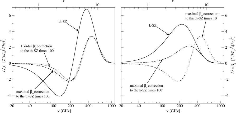
Figure 1: Frequency-dependence of the SZ brightness due the non-relativistic th- and k-SZ and the corresponding corrections induced by the motion of the Solar System relative to the CMB rest frame for a cluster with electron temperature $k\,T_{\rm e}=5.1\,$keV, which is moving with ${\beta_{\rm c}}=10^{-3}$ towards the observer and is located at the maximum of the CMB dipole, i.e. ${\beta_{\rm o,\parallel}}=1.241\cdot 10^{-3}$. In addition the first order ${\beta_{\rm c}}$ correction to the th-SZ (dash-dotted line in the left panel) is shown. Note that for convenience all the velocity corrections are multiplied by some factor as given in the labels.

Transformation of the measured flux

The spectral flux $F(\nu,\mbox{\boldmath${n}$\unboldmath}_{0})$ from a solid angle area $\mathcal{A}$ in the direction $\mbox{\boldmath${n}$\unboldmath}_{0}$ on the sky in $S$ is given by the integral $F(\nu,\mbox{\boldmath${n}$\unboldmath}_{0})=\int\nolimits_{\mathcal{A}}I(\nu,\mbox{\boldmath${n}$\unboldmath})\,\mu_{0}{\,\rm d}\Omega$, where we defined $\mu_{0}=\mbox{\boldmath${n}$\unboldmath}\cdot\mbox{\boldmath${n}$\unboldmath}_{0}$. If one assumes that the angular dimension of $\mathcal{A}$ is small, then using (3a) in the observers frame $S^{\prime}$ the change of the flux due to Doppler boosting and aberration is given by

$$\Delta F^{\prime}_{\rm D}(\nu^{\prime},\mbox{\boldmath${n}$\unboldmath}^{\prime}_{0}) \approx{\beta_{\rm o,\parallel}}\,\left[3-\nu^{\prime}\partial_{\nu^{\prime}}\right]F(\nu^{\prime},\mbox{\boldmath${n}$\unboldmath}^{\prime}_{0})$$ (4a)

$$\Delta F^{\prime}_{\rm A}(\nu^{\prime},\mbox{\boldmath${n}$\unboldmath}^{\prime}_{0}) \approx{\beta_{\rm o,\parallel}}\,\int\nolimits_{\mathcal{A}}\,\theta^{\prime 2}\,\partial_{\theta^{\prime}}I(\nu^{\prime},\mbox{\boldmath${n}$\unboldmath}^{\prime}){\,\rm d}\theta^{\prime}{\,\rm d}\phi^{\prime}\,.$$ (4b)

Assuming that the area $\mathcal{A}$ contains an unresolved object, which contributes most of the total flux and vanishes on the boundaries of the region, then the term arising due to aberration only can be rewritten as

$$\Delta F^{\prime}_{\rm A}(\nu^{\prime},\mbox{\boldmath${n}$\unboldmath}^{\prime}_{0}) =-2\,{\beta_{\rm o,\parallel}}\,F(\nu^{\prime},\mbox{\boldmath${n}$\unboldmath}^{\prime}_{0})\,.$$ (5)

This can be simply understood considering that in the direction of the motion the solid angle covered by an object is smaller by a factor $[1-{\beta_{\rm o,\parallel}}]^{2}\approx 1-2\,{\beta_{\rm o,\parallel}}$. In this case the total change in the spectral flux $F^{\prime}(\nu^{\prime},\mbox{\boldmath${n}$\unboldmath}^{\prime}_{0})$ is

$$\frac{\Delta F}{F}=\frac{F^{\prime}(\nu^{\prime},\mbox{\boldmath${n}$\unboldmath}^{\prime}_{0})-F(\nu^{\prime},\mbox{\boldmath${n}$\unboldmath}^{\prime}_{0})}{F(\nu^{\prime},\mbox{\boldmath${n}$\unboldmath}^{\prime}_{0})}={\beta_{\rm o,\parallel}}\left[1-\frac{\displaystyle\partial\ln F}{\displaystyle\partial\ln\nu^{\prime}}\right]\,.$$ (6)

Integrating the flux $F^{\prime}(\nu^{\prime},\mbox{\boldmath${n}$\unboldmath}^{\prime}_{0})$ over frequency $\nu^{\prime}$ it is straightforward to obtain the change of the total bolometric flux $F^{\prime}_{\rm bol}(\mbox{\boldmath${n}$\unboldmath}^{\prime}_{0})=\int F^{\prime}(\nu^{\prime},\mbox{\boldmath${n}$\unboldmath}^{\prime}_{0}){\,\rm d}\nu^{\prime}$ in the observers frame $S^{\prime}$:

$$\frac{\Delta F_{\rm bol}}{F_{\rm bol}}=\frac{F^{\prime}_{\rm bol}(\mbox{\boldmath${n}$\unboldmath}^{\prime}_{0})-F_{\rm bol}(\mbox{\boldmath${n}$\unboldmath}^{\prime}_{0})}{F_{\rm bol}(\mbox{\boldmath${n}$\unboldmath}^{\prime}_{0})}=2\,{\beta_{\rm o,\parallel}}\,.$$ (7)

This results can also be easily understood considering the transformation law for the total bolometric intensity $I_{\rm bol}=\int I(\nu){\,\rm d}\nu$, i.e. $I^{\prime}_{\rm bol}=I_{\rm bol}/[\gamma(1-{\beta_{\rm o}}\mu^{\prime})]^{4}$, and the transformation of the solid angle ${\,\rm d}\Omega^{\prime}=[\gamma(1-{\beta_{\rm o}}\mu^{\prime})]^{2}{\,\rm d}\Omega$.

Transformation of the number counts

Defining $\frac{{\,\rm d}N}{{\,\rm d}\Omega}(F,\@vec{n})$ as the number of objects per solid angle ${\,\rm d}\Omega$ above a given flux $F$ at some fixed frequency $\nu$ and in some direction $\@vec{n}$ on the sky in the CMB rest frame $S$, then the corresponding quantity in the observers frame $S^{\prime}$ is given by

$$\frac{{\rm d}N^{\prime}}{{\rm d}\Omega^{\prime}}(F^{\prime},\@vec{n}^{\prime}) =\frac{{\rm d}N}{{\rm d}\Omega}(F,\@vec{n})\,\frac{{\rm d}\Omega}{{\rm d}\Omega^{\prime}}\,,$$ (8)

where $F$ and ${n}$ are functions of $F^{\prime}$ and $\mbox{\boldmath${n}$\unboldmath}^{\prime}$. Now, assuming isotropy in $S$, in first order of ${\beta_{\rm o,\parallel}}$ one may write

$$\frac{{\rm d}N^{\prime}}{{\rm d}\Omega^{\prime}}(F^{\prime},\@vec{n}^{\prime})\approx\frac{{\rm d}N}{{\rm d}\Omega}(F^{\prime})\\ \times\left[1+2\,{\beta_{\rm o,\parallel}}-\frac{\Delta F}{F}\,\frac{\partial\ln\frac{{\rm d}N}{{\rm d}\Omega}(F^{\prime})}{\partial\ln F^{\prime}}\right]\,,$$ (9)

with $\Delta F=F^{\prime}-F$. For unresolved objects $\Delta F/F$ is given by equation (6). Here we made use of the transformation law for the solid angles and performed a series expansion of $\frac{{\,\rm d}N}{{\,\rm d}\Omega}(F)$ around $F^{\prime}$.

If one assumes $\frac{{\,\rm d}N}{{\,\rm d}\Omega}(F)\propto F^{-\lambda}$ and $F(\nu)\propto\nu^{-\alpha}$, it is straightforward to show that for unresolved sources $\frac{{\,\rm d}N^{\prime}}{{\,\rm d}\Omega^{\prime}}(F^{\prime},\@vec{n}^{\prime})\approx\frac{{\,\rm d}N}{{\,\rm d}\Omega}(F^{\prime})\left[1+{\beta_{\rm o,\parallel}}(2+\lambda[1+\alpha])\right]$. This result was obtained earlier by Ellis & Baldwin (1984) for the change of the radio source number counts due to the motion of the observer. Dependent on the sign of the quantity $\Sigma=2+\lambda[1+\alpha]$ there is an increase or decrease in the number counts in one given direction. However, in the case of clusters $\alpha$ is a strong function of frequency, which makes the situation more complicated.

3 Transformation of the cluster signal

For an observer at rest in the frame $S$ defined by the CMB the change of the surface brightness in the direction $\@vec{n}$ towards a cluster of galaxies is given by the sum of the signals due to the th-SZ, ${I_{\,\rm th}}(\nu,\@vec{n})$ and the k-SZ, ${I_{\,\rm k}}(\nu,\@vec{n})$:

$${I_{\,\rm SZ}}(\nu,\@vec{n})={I_{\,\rm th}}(\nu,\@vec{n})+{I_{\,\rm k}}(\nu,\@vec{n})\,.$$ (10)

In the non-relativistic case these contributions are given by (see Zeldovich & Sunyaev, 1969; Sunyaev & Zeldovich, 1980a, b):

$${I_{\,\rm th}}(\nu,\@vec{n}) =y\,\frac{x\,e^{x}}{e^{x}-1}\left[x\,\frac{e^{x}+1}{e^{x}-1}-4\right]I_{0}(\nu)$$ (11a)

$${I_{\,\rm k}}(\nu,\@vec{n}) =\tau\,{\beta_{\rm c,\parallel}}\,\frac{x\,e^{x}}{e^{x}-1}\,I_{0}(\nu)\,,$$ (11b)

where $I_{0}(\nu)=\frac{2h}{c^{2}}\,\frac{\nu^{3}}{e^{x}-1}$ denotes the CMB monopole intensity with temperature $T_{0}$, $y=\int\frac{k\,T_{\rm e}}{m_{\rm e}c^{2}}\,n_{\rm e}\,\sigma_{\rm T}{\,\rm d}l$ is the Compton $y$-parameter, with the electron number density $n_{\rm e}$, and we introduced the abbreviation $x=h\nu/k\,T_{0}$. Here we are only interested in the correction to the intensity in the central region of the cluster, where the spatial derivative of $y$ is small and the effects of aberration may be neglected. Using equations (3b) and (11) one may find

$${\Delta I^{\prime}_{\rm D,th}}(\nu^{\prime},\@vec{n}^{\prime}) =y\,I_{0}(\nu^{\prime})\,\frac{x^{\prime}e^{x^{\prime}}}{e^{x^{\prime}}-1}\,{\mathcal{C}_{\rm th}}(x^{\prime})\cdot{\beta_{\rm o}}\,\mu^{\prime}$$ (12a)

$${\Delta I^{\prime}_{\rm D,k}}(\nu^{\prime},\@vec{n}^{\prime}) =\tau\,{\beta_{\rm c,\parallel}}\,I_{0}(\nu^{\prime})\,\frac{x^{\prime}e^{x^{\prime}}}{e^{x^{\prime}}-1}\,{\mathcal{C}_{\rm k}}(x^{\prime})\cdot{\beta_{\rm o}}\,\mu^{\prime}$$ (12b)

for motion-induced change of the cluster brightness. Here the functions ${\mathcal{C}_{\rm th}}({\hat{x}})$ and ${\mathcal{C}_{\rm k}}({\hat{x}})$ are defined by

$${\mathcal{C}_{\rm th}}({\hat{x}}) =4-6\,\mathcal{X}+\mathcal{X}^{2}+\frac{1}{2}\mathcal{S}^{2}$$ (13a)

$${\mathcal{C}_{\rm k}}({\hat{x}}) =\mathcal{X}-1$$ (13b)

and the notations $\mathcal{X}=x\,\coth(\frac{x}{2})$, $\mathcal{S}=x/\sinh(\frac{x}{2})$ were introduced.

In Fig. 1 the spectral dependence of ${\Delta I^{\prime}_{\rm D,th}}$ and ${\Delta I^{\prime}_{\rm D,k}}$ is illustrated. The transformation of the th-SZ leads to a spectral distortion which is very similar to the first order ${\beta_{\rm c}}$ correction to the th-SZ. In the Rayleigh-Jeans limit ${\mathcal{C}_{\rm th}}({\hat{x}})\rightarrow-2$ and therefore is 5 times bigger than the ${\beta_{\rm c}}$ correction to the th-SZ. The maximum/minimum of ${\Delta I^{\prime}_{\rm D,th}}$ is at $x=7.97\,/\,3.31$ and ${\Delta I^{\prime}_{\rm D,th}}$ vanishes at $x=5.10$ ($x=1$ corresponds to $\nu=56.8\,$GHz). On the other hand the transformation of the k-SZ leads to a y-type spectral distortion with the corresponding y-parameter ${y_{\rm kin}}=\tau\,{\beta_{\rm c,\parallel}}\,{\beta_{\rm o}}\,\mu^{\prime}\sim 10^{-8}\,\mu^{\prime}$. The maximum of ${\Delta I^{\prime}_{\rm D,k}}$ is at $x=5.10$. Fig. 1 clearly shows, that the motion-induced correction to the th-SZ easily reaches the level of a few percent in comparison to the k-SZ (e.g. at $\nu=400\,$GHz it contributes $\sim 14$% to the k-SZ signal for a cluster with $k\,T_{\rm e}=5.1\,$keV and ${\beta_{\rm c}}=10^{-3}$).

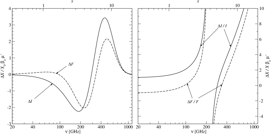
Figure 2: Motion-induced change of the CMB spectral brightness $\Delta I$ and flux $\Delta F$ for a cluster of galaxies resting with respect to the CMB. Left panel: Absolute change of the cluster brightness (solid line) with $X_{0}=2.70\times 10^{11}\,y\,$mJy/sr and the flux for an unresolved cluster (dashed line) with $X_{0}=7.17\,\left<y/10^{-4}\,r_{\rm c}^{2}\right>_{\rm cl}(r_{\rm c}/30^{\prime\prime})^{2}\,$mJy, where $r_{\rm c}$ is the core radius and where $\left<u\right>_{\rm cl}=\int_{\rm cl}u{\,\rm d}\Omega/4\pi$ denotes the cluster average of the quantity $u$. Right panel: Relative change of the brightness (solid line) and flux for an unresolved cluster (dashed line). Here $\Delta I/I={\beta_{\rm o}}\,\mu^{\prime}\,(3+\alpha)$ and $\Delta F/F={\beta_{\rm o}}\,\mu^{\prime}\,(1+\alpha)$ (cf. Equ. (15)).

In order to obtain the motion-induced change of the flux for unresolved clusters one has to integrate the surface brightness over the surface of the cluster. In the following we neglect the k-SZ, since its contribution only becomes important close to the crossover frequency. Then it follows that $\Delta F(\nu,\@vec{n})\propto\Delta I(\nu,\@vec{n})$, implying that ${\,\rm d}\ln F/{\,\rm d}\ln\nu^{\prime}={\,\rm d}\ln I/{\,\rm d}\ln x^{\prime}$. Comparing equations (3b) and (12) one can define the effective spectral index of the SZ signal by

$$\alpha=-\frac{{\,\rm d}\ln F(x^{\prime})}{{\,\rm d}\ln x^{\prime}}=\frac{{\mathcal{C}_{\rm th}}(x^{\prime})}{Y_{0}(x^{\prime})}-3\,,$$ (14)

with $Y_{0}(x)=\mathcal{X}-4$. Using equation (14) one can write the central brightness, flux and number count for unresolved clusters as

$${I^{\prime}_{\,\rm SZ}}(\nu^{\prime},\@vec{n}^{\prime}) ={I_{\,\rm SZ}}(\nu^{\prime},\@vec{n}^{\prime})\,\left[1+{\beta_{\rm o}}\,\mu^{\prime}(3+\alpha)\right]$$ (15a)

$${\Delta F^{\prime}_{\,\rm SZ}}(\nu^{\prime},\@vec{n}^{\prime}) ={\Delta F_{\,\rm SZ}}(\nu^{\prime},\@vec{n}^{\prime})\,\left[1+{\beta_{\rm o}}\,\mu^{\prime}(1+\alpha)\right]$$ (15b)

$$\frac{{\,\rm d}N^{\prime}_{\rm SZ}}{{\,\rm d}\Omega^{\prime}}(F^{\prime},\@vec{n}^{\prime}) =\frac{{\,\rm d}N_{\rm SZ}}{{\,\rm d}\Omega}(F^{\prime})\,\left[1+{\beta_{\rm o}}\,\mu^{\prime}\Sigma\right]\,,$$ (15c)

with $\Sigma=2+\lambda(1+\alpha)$ and $\lambda=-\frac{\partial\ln\frac{{\,\rm d}N}{{\,\rm d}\Omega}(F^{\prime})}{\partial\ln F^{\prime}}$. Fig. 2 shows the change of the central brightness and the flux for an unresolved cluster. It is obvious that only in the RJ region of the CMB spectrum the SZ brightness and flux follow a power-law. The change of the number counts will be discussed below (see Sect. 4.1).

4 Multi-frequency observations of clusters

The observed CMB signal in the direction of a cluster consists of the sum of all the contributions mentioned above, including the relativistic correction to the SZ effect. Given a sufficient frequency coverage and spectral sensitivity one may in principle model the full signal for even one single cluster, but obviously there will be degeneracies which have to be treated especially if noise and foregrounds are involved. Therefore it is important to make use of the special properties of each contribution to the total signal, such as their spectral features and spatial dependencies.

One obstacle for any multi-frequency observation of cluster is the cross-calibration of different frequency channels. Some method to solve this problem was discussed in Chluba & Sunyaev (2004) using the spectral distortions induced by the superposition of blackbodies with different temperatures. In the following we assume that the achieved level of cross-calibration is sufficient.

The largest CMB signal in the direction of a cluster (after elimination of the CMB dipole) is due to the th-SZ. In order to handle this signal one can make use of the zeros of the spectral functions describing the relativistic corrections. In addition, future X-ray spectroscopy will allow us to accurately determine the mean temperature of the electrons inside clusters. This additional information will place useful constraints on the parameters describing the th-SZ and therefore may bring us down to the effects connected with the peculiar velocities of the cluster and the observer.

The temperature difference connected with the non-relativistic k-SZ is frequency-independent and therefore may be eliminated by multi-frequency observations. As mentioned above (see Fig. 1) the motion-induced spectral distortion to the th-SZ has an amplitude and spectral dependence, which is very similar to the effect connected with the first order ${\beta_{\rm c}}$ correction to the th-SZ. For many clusters on the other hand one can expect that the signals proportional to ${\beta_{\rm c,\parallel}}$ average out. This implies that for large cluster samples ($\sim 10^{3}-10^{4}$) only the signals connected with the th-SZ are important.

4.1 Dipolar asymmetry in the number of observed clusters

Integrating (15c) over solid angle leads to the observed number of clusters in a given region of the sky. If one assumes that the observed region is circular with radius ${\theta^{\prime}_{\rm r}}$ centered in the direction $\mbox{\boldmath${n}$\unboldmath}_{0}^{\prime}=(\phi^{\prime}_{0},\theta_{0}^{\prime})$ then the total observed number of clusters is given by

$$N^{\prime}_{\rm SZ}(F^{\prime}) =N_{\rm SZ,eff}(F^{\prime})\,\left[1+{\beta_{\rm o}}\,\mu^{\prime}_{0}\,\frac{1+{\mu^{\prime}_{\rm r}}}{2}\,\Sigma\right]\,,$$ (16)

where $N_{\rm SZ,eff}(F^{\prime})=4\pi\,\frac{{\,\rm d}N_{\rm SZ}}{{\,\rm d}\Omega}\,\frac{1-{\mu^{\prime}_{\rm r}}}{2}$ is the effective number of clusters inside the observed patch with fluxes above $F^{\prime}$, ${\mu^{\prime}_{\rm r}}=\cos{\theta^{\prime}_{\rm r}}$ and $\mu_{0}^{\prime}=\cos\theta_{0}^{\prime}$. For two equally sized patches in separate directions on the sky the difference in the number of observed clusters will then be

$$\Delta N^{\prime}={\beta_{\rm o}}\,N_{\rm SZ,eff}\,\Delta\mu^{\prime}_{0}\,\frac{1+{\mu^{\prime}_{\rm r}}}{2}\,\Sigma\,,$$ (17)

with $\Delta\mu^{\prime}_{0}=\mu^{\prime}_{0,1}-\mu^{\prime}_{0,2}$, where $\mu^{\prime}_{0,i}=\cos\theta_{0,i}^{\prime}$ for patch $i$. Centering the first patch on the maximum and the second on the minimum of the CMB dipole leads to the maximal change in the number of observed clusters at a given frequency ($\Delta\mu^{\prime}_{0}=2$). To estimate the significance of this difference we compare $\Delta N^{\prime}$ to the Poissonian noise in the number of clusters for both patches, which is given by $\sqrt{N^{\prime}_{\rm SZ,1}+N^{\prime}_{\rm SZ,2}}\approx\sqrt{2\,N_{\rm SZ,eff}}$. To obtain a certain signal to noise level $q$ the inequality

$${\beta_{\rm o}}\,|\Sigma|\,\Delta\mu^{\prime}_{0}\,[1+{\mu^{\prime}_{\rm r}}]\,\sqrt{1-{\mu^{\prime}_{\rm r}}}\geq\frac{4\,q}{\sqrt{N_{\rm SZ,f}}}$$ (18)

has to be fulfilled. We defined $N_{\rm SZ,f}=4\pi\,\frac{{\,\rm d}N_{\rm SZ}}{{\,\rm d}\Omega}$ as the number of clusters on the whole sky above a given flux level $F^{\prime}$. Here two effects are competing: the smaller the radius of each patch, the smaller the number of observed clusters above a given flux but the larger the effective $\left<{\beta_{\rm o,\parallel}}\right>$. The optimal radius is ${\theta_{\rm r}}\sim\leavevmode\nobreak\ 70^{\circ}$ but for a given $q$ and sensitivity the size in principle can be smaller.

4.2 Numerical estimates for the dipolar asymmetry in the cluster number counts

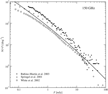
Figure 3: $\log N$-$\log F$: Number of clusters per square degree with flux level above $F$ at observing frequency $\nu=150\,$GHz. The solid line shows the modified Press-Schechter prescription as used in this work.

In this section we present results for the SZ cluster number counts using a simple Press-Schechter (Press & Schechter, 1974) prescription for the mass function of halos as modified by Sheth et al. (2001) to include the effects of ellipsoidal collapse. Since we are interested in unresolved objects we only need to specify the cluster mass-temperature relation and baryonic fraction. For the former we apply the frequently used scaling relation and normalization as given by Bryan & Norman (1998), whereas for the latter we simply assume a universal value of $\Omega_{\rm b}/\Omega_{\rm m}$, which is rather close to the local values as derived from X-ray data (e.g. Mohr et al., 1994) independent of cluster mass and redshift. We note that these two assumptions are the biggest source of uncertainty in our calculations and the use of them is only justified given the lack of current knowledge about the detailed evolution of the baryonic component in the Universe. In spite of these gross simplifications our results on cluster number counts agree very well with those obtained in state-of-the-art hydrodynamical simulations by Springel et al. (2001) and White et al. (2002) as demonstrated in Fig. 3. Here the counts are calculated for the $\Lambda$CDM concordance model (Spergel et al., 2003) assuming observing frequency of $150\,$GHz. The first set of simulations included only adiabatic gas physics whereas for the second also gas cooling and feedback from supernovae and galactic winds was taken into account. We also plot the results obtained by Rubiño-Martín & Sunyaev (2003) using a Monte-Carlo simulations based on a Press-Schechter approach. In the estimates presented below we will use the curve given by the solid line in Fig.3, which in the most interesting range of lower flux limits ($1\,$mJy -$10\,$mJy) has an effective power-law slope of $\lambda\sim 1.10-1.25$.

In Fig. 4 we compare the motion-induced dipolar asymmetry in number counts as a function of the observing frequency using the optimal patch radius $\theta_{\rm r}=70^{\circ}$ for both sides of the sky with the $1\sigma$ Poisson noise level for the two lower flux limits of $1\,$mJy and $10\,$mJy. In addition we mark the regions where we expect an increase of the number of negative sources and a decrease/increase of the number of positive sources, respectively, if one is observing only in the direction of the maximum of the CMB dipole. It is important to note that the motion-induced change in the cluster number counts vanishes at frequencies $\nu\sim\leavevmode\nobreak\ 300\,$GHz. The exact value of this frequency depends both on the slope of the number count curve and the spectral index.

Fig. 5 presents the sensitivity limits where the motion-induced signal is equal to the $3\sigma$ and $5\sigma$ Poissonian noise levels for different observing frequencies. Taking into account that new generation of SZ dedicated surveys (e.g. Spt and Act) will have mJy sensitivities, we see that for experiments covering the full sky a detection of the motion-induced signal is clearly within the reach of the capabilities of modern technology especially at frequencies in the range $\nu=400-500\,$GHz. Combining the data of different experiments with limited sky coverage may lead to a sufficient total sample (see Fig. 6).

It is important to mention that in our simplistic calculations we assumed that all the clusters remain unresolved, which is a good approximation for the Planck, Spt and Act. For experiments with higher angular resolution a significant population of clusters will be resolved and hence the number count curves presented here will change accordingly.

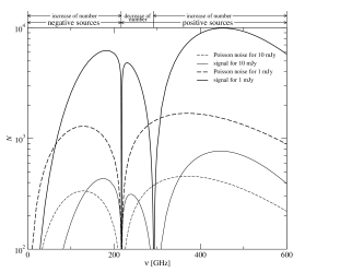
Figure 4: Motion-induced dipolar asymmetry in number counts (solid lines) as a function of the observing frequency using the optimal patch radius $\theta_{\rm r}=70^{\circ}$ for both patches, where the first is centered on the maximum, the second on the minimum of the CMB dipole. For comparison we give the corresponding $1\sigma$ Poissonian noise level (dashed curves). In addition we mark the regions where we expect an increase of the number of negative sources and a decrease/increase of the number of positive sources, respectively, if one is observing only in the direction of the maximum of the CMB dipole.

From Fig. 5 we also see that the most promising frequencies for a detection of the motion-induced asymmetries are around the crossover frequency (i.e.$\sim 217\,$GHz) and in the range $\nu\sim 400-500\,$GHz. Clearly, for a proper modeling near the crossover frequency one has to take into account the contribution from the k-SZ, which has been neglected so far. It is evident that the k-SZ is contributing symmetrically to channels around $217\,$GHz in the sense that the number of positive and negative sources is approximately equal. On the other hand in the range $\nu\sim 400-500\,$GHz other astrophysical source start to contribute to the source counts (see Sect. 4.3).

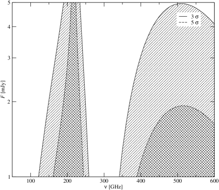
Figure 5: Required sensitivities for a $3\sigma$ and $5\sigma$-detection of the motion-induced dipolar asymmetry in number counts as a function of frequency. The shaded areas indicate regions where a detection above $3\,\sigma$ and $5\,\sigma$ level is possible, respectively.

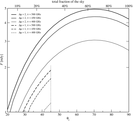
Figure 6: Required sensitivity limits for a $3\sigma$ detection of the number count asymmetry in the frequency range $400-500\,$GHz as a function of patch radius. One patch is centered on the maximum of the CMB dipole. Note that for $\Delta\mu=1$ and $\theta_{\rm r}>\leavevmode\nobreak\ 45^{\circ}$ the two patches start to overlap and therefore the corresponding curves were not presented here.

Finally, in Fig. 6 we illustrate the dependence of the required sensitivities for a $3\sigma$ detection of the number count asymmetry on the radius of the two compared patches close to the frequency $\nu\sim 500\,$GHz. The first patch is centered on the maximum of the CMB dipole, whereas for the second we choose the two cases $\theta_{0,2}=90^{\circ}$ and $180^{\circ}$, i.e. $\Delta\mu_{0}=1$ and $2$, respectively. This Figure shows that for frequencies below $\sim 400-500\,$GHz and separation angles smaller than $90^{\circ}$ a detection of the asymmetry will only be feasible for experiments with sub-mJy sensitivity.

4.3 Source count contribution from non-SZ populations

In the range $\nu\sim 400-500\,$GHz, which is most promising for a detection of the motion-induced number count asymmetry, other foreground sources begin to play a role, e.g. dusty high redshift galaxies (Blain et al., 2002). In the microwave band these galaxies have extremely peculiar spectrum $F(\nu)\propto\nu^{-\alpha_{\rm d}}$, with $\alpha_{\rm d}$ ranging from $-3$ to $-4$. Using formula (9) it is easy to show that the observed properties of this population will also be influenced by the motion of the Solar System, but in a completely different way than clusters: in the direction of our motion relative to the CMB rest frame their brightness and fluxes decrease when for clusters they increase. This implies that in the frequency range $\nu\sim 400-500\,$GHz the motion-induced dipolar asymmetry in the number counts for these sources has the opposite sign in comparison to clusters, i.e. $\Delta N^{\prime}_{\rm d}<0$ when $\Delta N^{\prime}_{\rm cl}>0$. Detailed multi-frequency observations should allow distinguishing the source count contributions of these two classes of objects, but nevertheless it is interesting that they a different sign of the motion-induced flux dipole.

5 Conclusion

In this paper we derived the changes to the SZ cluster brightness, flux and number counts induced by the motion of the Solar System with respect to the CMB rest frame. These corrections to the SZ cluster brightness and flux have similar spectral behavior and amplitude as the first order velocity correction to the th-SZ (see Fig. 1) and thus need to be taken into account for the precise modeling of the cluster signal. Since both the amplitude and direction of the motion of the Solar System is known with a high precision it is easy to correct for these changes.

The dipolar asymmetry induced in the SZ cluster number counts in contrast to the counts of more conventional sources can change polarity dependent on the observational frequency (see Sect. 4.3). This behavior is due to the very specific frequency dependence of the SZ effect. We find that frequencies around the crossover frequency $\sim 217$ GHz and in the range $\sim 400-500$ GHz are the most promising for a detection of this motion-induced number count asymmetry (see Fig. 5).