Testing for double inflation with WMAP

Abstract

With the WMAP data we can now begin to test realistic models of inflation involving multiple scalar fields. These naturally lead to correlated adiabatic and isocurvature (entropy) perturbations with a running spectral index. We present the first full (9 parameter) likelihood analysis of double inflation with WMAP data and find that despite the extra freedom, supersymmetric hybrid potentials are strongly constrained with less than $7\%$ correlated isocurvature component allowed when standard priors are imposed on the cosomological parameters. As a result we also find that Akaike & Bayesian model selection criteria rather strongly prefer single-field inflation, just as equivalent analysis prefers a cosmological constant over dynamical dark energy in the late universe. It appears that simplicity is the best guide to our universe.

I Introduction

Our universe shows evidence of complexity and, at the same time, great simplicity. Our universe appears entirely consistent with being a “double-de Sitter sandwich” - radiation and matter dominated phases caught between two de Sitter phases at low and high energies respectively.

Recent work jochen ; params has shown that a cosmological constant provides a better fit than dynamical dark energy to current CMB and SNIa data if one computes the Bayesian evidence or uses information criteria for model selection. In this paper we will show that, at least within a class of double, hybrid inflation models, the same is true for the early universe. One might envisage various infrared-ultraviolet dualities to explain such behaviour.

Despite this apparent “asymptotic blandness ” there is interesting tentative evidence to the contrary. The WMAP data show unusual characteristics such as “oscillations” oscil which may disappear with more data or may be the first signs of new physics. Similarly there is evidence for a feature in the power spectrum feature which can easily be produced by the subtle dynamics of multiple light scalar fields during inflation.

Multiple light fields during inflation automatically widens the narrow predictions of single-field inflation for now there are multiple entropy perturbations PS -GV which are, in general, correlated to some degree with the standard adiabatic mode Langlois -Crotty . Correlations are produced when the valley of the effective potential is curved Gordon and this also leads to non-gaussianity nongauss . Since the effective masses of the various fields typically depend on the vacuum expectation values of the other (dynamical) fields these are time-dependent and can cause violations of standard slow-roll conditions and spectral indices for the perturbations which run with scale Tsuji .

This is a crucial aspect of this present work because previous analyses of correlated adiabatic and entropy (isocurvature) perturbations have always assumed power-law spectra for all the perturbations Amen ; BMT ; WM ; VM ; Crotty . When applied to the WMAP data they found that with standard priors on cosmological parameters the degree of correlation allowed is small (although see cons ). Allowing running of the spectral index, at least in the supersymmetric hybrid models we study, does not change this conclusion.

The code we have developed allows us to numerically study any inflationary model without approximation (except in the treatment of spinodal/tachyonic instabilities) and builds on that used in Tsuji . Future work will consider more fields where sharp features can occur, something which does not occur in the two-field double-inflation models we study here.

II General formalism

We consider two minimally coupled scalar fields, $\phi$ and $\chi$, with an effective potential $V(\phi,\chi)$. Our main interest is the case of double inflation in which two stages of inflation are realized. General scalar metric perturbations about the flat Friemann-Lemaitre-Robertson-Walker background can be written as (see e.g. Gordon )

$$ds^{2} = -(1+2A)dt^{2}+2a(t)B_{,i}dx^{i}dt$$

$$+a^{2}(t)[(1-2\psi)\delta_{ij}+2E_{,ij}]dx^{i}dx^{j}\,,$$

where $a(t)$ is the scale factor. The comoving curvature perturbation in our two-field system is then given by

$${\cal R}\equiv\psi+\frac{H(\dot{\phi}\delta\phi+\dot{\chi}\delta\chi)}{\dot{\phi}^{2}+\dot{\chi}^{2}}\,,$$ (2)

where $H\equiv\dot{a}/a$ is a Hubble rate, and $\delta\phi$ and $\delta\chi$ are the perturbations of the fields $\phi$ and $\chi$, respectively.

The perturbation equations are given in Refs. Gordon ; Bartolo and one can numerically evaluate the power spectrum, ${\mathcal{P}}_{{\cal R}}\equiv(k^{3}/2\pi^{2})|{\cal R}|^{2}$, at the end of inflation Tsuji (here $k$ is comoving momentum). In the multi-field system we also need to account for the spectra of isocurvature perturbations, ${\mathcal{P}}_{S}$, and correlated adiabatic and isocurvature perturbations, ${\mathcal{P}}_{C}$ (see Ref. Bartolo ; Tsuji for their definitions). The quantity $r_{C}$ defined by $r_{C}={\mathcal{P}}_{C}/\sqrt{{\mathcal{P}}_{\mathcal{R}}{\mathcal{P}}_{S}}$ is the measure of the strength between adiabatic and isocurvature perturbations.

The system possesses several model parameters associated with the potential. We assume slow-roll conditions apply $|\ddot{\phi}|\ll|3H\dot{\phi}|$ and $|\ddot{\chi}|\ll|3H\dot{\chi}|$, for the initial conditions of background fields, so that the $\ddot{\phi}$ and $\ddot{\chi}$ terms are neglected. Then the initial conditions of $\dot{\phi}$ and $\dot{\chi}$ are determined by $\phi_{\rm in}$ and $\chi_{\rm in}$ (the subscript “in” denotes the initial values). We perform the likelihood analysis over the initial conditions $\phi_{\rm in}$, $\chi_{\rm in}$.

Note that the number of inflationary model parameters depends explicitly on the inflaton potential and typically requires at least three parameters in the context of double inflation.

We impose the condition that the total number of $e$-folds during inflation must exceed $N_{\rm T}=50$ to solve flatness and horizon problems. We find the cosmologically relevant perturbation modes with comoving wavenumbers $k$ and numerically evolve the background and all perturbation equations through inflation, giving us the three power spectra $({\mathcal{P}}_{{\cal R}},{\mathcal{P}}_{S},{\mathcal{P}}_{C})$, as described in Tsuji .

It is important to solve the perturbation equations without approximation right up to the end of inflation, since the curvature perturbation is not necessarily conserved after Hubble radius crossing GW , unlike the case of single-field inflation.

The resulting data: $P_{i}=\log{\mathcal{P}}(k_{i})$ given at a wave number of $x_{i}=\log k_{i}$, $i=1,..m$, are optimally fitted with a polynomial function $P_{\rm fit}(x)=a+bx+cx^{2}$ by minimizing $\bar{\chi}^{2}=\sum_{i}(a+bx_{i}+cx_{i}^{2}-P_{i})^{2}$.

For each set of parameters we derive the best-fit coefficients $a,b,c$ for each of the three power spectra. It is worth mentioning that the coefficients $b$ and $c$ are intimately linked to the spectral index $n_{s}$ and its running of scalar perturbations by the relations $n_{s}=b+1$ and $\alpha_{s}=2c$. We check that our fitting method agrees very well with numerically obtained power spectra and is sufficient to accurately capture any running of the spectral index over cosmologically relevant scales.

We assume, as is standard, that the field $\phi$ decays to ordinary matter like photons, neutrinos and baryons, whereas the field $\chi$ decays into cold dark matter (CDM) Langlois ; Gordon . In this case the mixing between two scalar fields is negligible and the CDM isocurvature perturbations and correlations remain after reheating. Relaxing this assumption will introduce extra parameters into the analysis.

The CMB temperature anisotropies are given in general by

$$C_{\ell}=(4\pi)^{2}\int k^{2}dk\Delta_{\ell}^{2}\langle k,\tau_{0}\rangle,$$ (3)

where $\Delta_{\ell}(k,\tau_{0})$ is the $\ell$-multipole of the $k$-th wavenumber temperature anisotropy at the present time $\tau_{0}$. For a general set of correlated initial conditions, one has

$$\Delta(k,\tau_{0})=P_{\mathcal{R}}^{1/2}\Delta_{\mathcal{R}}(k,\tau_{0})+P_{S}^{1/2}\Delta_{S}(k,\tau_{0}),$$ (4)

where $\langle\Delta_{\mathcal{R}}^{2}(k,\tau_{\rm in})\rangle=\langle\Delta_{S}^{2}(k,\tau_{\rm in})\rangle=1$ and $\langle\Delta_{\mathcal{R}}(k,\tau_{\rm in})\Delta_{S}(k,\tau_{\rm in})\rangle=r_{C}$. Then we get

$$C_{\ell} = (4\pi)^{2}\int k^{2}dk[P_{\mathcal{R}}\Delta_{\ell,\mathcal{R}}^{2}+P_{S}\Delta_{\ell,S}^{2}+2r_{c}\langle\Delta_{\ell,\mathcal{R}}\Delta_{\ell,S}\rangle]$$ (5)

$$\equiv C_{\ell,\mathcal{R}}+C_{\ell,S}+2C_{\ell,C}\,.$$

It is possible to obtain the three multipole spectra required for any general set of initial perturbations using the following simple scheme. Let us denote $C(A_{1},A_{2})$ as the $C_{\ell}$ spectrum obtained with completely correlated initial conditions with a given adiabatic spectrum $A_{1}$ and given isocurvature spectrum $A_{2}$. A typical Boltzmann code can produce only $C(A_{1},0)$ (pure adiabatic), $C(0,A_{2})$ (pure isocurvature) or $C(A_{1},A_{1})$ (completely correlated mixture of adiabatic and isocurvature with the same initial spectrum). It is not difficult to see that the general spectrum is given by:

$$C(A_{1},A_{2}) = C(A_{1},0)+C(0,A_{2})+2[C(A_{12},A_{12})$$ (6)

$$-C(0,A_{12})-C(A_{12},0)]\,,$$

where in our case $A_{12}=\sqrt{P_{C}}$ , $A_{1}=\sqrt{P_{\mathcal{R}}}$ and $A_{2}=\sqrt{P_{S}}$. One needs therefore five evaluations for each combination of $P_{\mathcal{R},S,C}$. We make use of a modified version of the CAMB Boltzmann solver Lewis to evaluate the CMB power spectrum by this scheme.

In addition to $\phi_{\rm in}$, $\chi_{\rm in}$ and the inflationary potential parameters discussed in the next section, we varied 4 cosmological parameters: $\Omega_{b}h^{2}$, $\Omega_{c}h^{2}$, $\tau$, $H_{0}$; namely the baryon and cold dark matter density, the reionisation optial depth and the Hubble constant today. We assume spatial flatness, so $\Omega_{\Lambda}=1-\Omega_{b}-\Omega_{c}$.

It is well-known that the allowed ranges for these parameters has a large impact on the acceptable amount of correlated isocurvature perturbations cons2 . We choose fairly standard priors, allowing the above variables to vary in the ranges: $\tau\in[0,0.3]$, $H_{0}\in[50,90]$ with $\Omega_{b}$ and $\Omega_{c}$ both varying over the full unit interval, $[0,1]$. We choose very wide domains for $\phi_{\rm in}$ and $\chi_{\rm in}$ and found that the results depended very weakly on these boundaries.

We then use the first year WMAP TT and TE data Verde in our analysis to constrain the various parameters.

III A realistic double inflation model and likelihood results

Let us consider a fairly realistic multi-field inflation model with potential

$$V=\frac{\lambda}{4}\left(\chi^{2}-\frac{M^{2}}{\lambda}\right)^{2}+\frac{1}{2}g^{2}\phi^{2}\chi^{2}+\frac{1}{2}m^{2}\phi^{2}\,,$$ (7)

corresponding to the original version of the hybrid inflation Linde . This is closely linked with those obtained in supersymmetric theories Copeland ; Randall ; LR , which generically leads to a very strong correlation between the adiabatic and isocurvature perturbations due to the presence of a tachyonic instability between the two phases of inflation Tsuji . In this work we concentrate on the supersymmetric case with $g^{2}/\lambda=2$. Then we have three potential parameters: $\lambda$, $M$ and $m$, which are constrained by our likelihood analysis.

We can have two stages of inflation for the potential (7) depending upon the model parameters. One corresponds to the stage with $\phi>\phi_{c}\equiv M/g$ driven by the slow-roll evolution of $\phi$ during which the potential is approximately described by $V\simeq M^{4}/4\lambda+m^{2}\phi^{2}/2$. Another inflationary stage is the one with $\phi<\phi_{c}$ driven by the field $\chi$ with a tachyonic instability.

When the condition $M\gtrsim m$ is satisfied, then $M^{4}/\lambda\gtrsim m^{2}\phi_{c}^{2}$, and so the Hubble rate is roughly constant with a value $H=\sqrt{2\pi/3\lambda}M^{2}/m_{p}$, around $\phi=\phi_{c}$ (here $m_{p}$ is the Planck mass). We can estimate the condition for double inflation by estimating the effective masses of the two fields, i.e., $m_{\phi}^{2}\simeq m^{2}$ and $m_{\chi}^{2}\simeq g^{2}\phi^{2}-M^{2}$. Double inflation occurs when both of the masses of the two fields are smaller than $H$, which gives the condition

$$M^{2}\gtrsim mm_{p}\sqrt{3\lambda/2\pi}\,,$$ (8)

$$(M/m_{p})^{2}\gtrsim 3\lambda/2\pi\,.$$ (9)

We are mainly interested in the double inflation scenario in which the second stage of inflation occurs after the symmetry breaking. Since $m_{\chi}$ is smaller than $H$ around $\phi=\phi_{c}$, the field $\chi$ is hardly suppressed during the first stage of inflation, unless $\phi$ is not too much larger than $\phi_{c}$.

On the other hand, when $(M/m_{p})^{2}\ll\lambda$, the field $\chi$ is exponentially suppressed for $\phi>\phi_{c}$ and rapidly waterfalls toward the global minimum of the potential after symmetry breaking. This corresponds to the original version of the hybrid inflation without a second stage of inflation Linde .

In this case the homogeneous mode of $\chi$ can be vanishingly small relative to its fluctuations, so the analysis using linear perturbations is not fully trustworthy. In our work the linear perturbation equations in Ref. Tsuji are used to evaluate the three power spectra at the end of inflation. While the system is stable for the parameter range in which double inflation occurs, we found a strong numerical instability for perturbations in the tachyonic instability region when the field $\chi$ is strongly suppressed before symmetry breaking. Thus the latter case is effectively excluded from our analysis. In this case we need to account for the effect of diffusion using e.g., a Fokker Planck equation Randall ; Garcia , but we do not consider this here.

In order to constrain the double inflation model given by (7), we perform a likelihood analysis over 9 parameters: 5 inflationary $(M,\lambda,m,\phi_{\rm in},\chi_{\rm in})$ and 4 cosmological $(H_{0},\Omega_{b}h^{2},\Omega_{c}h^{2},\tau)$.

A grid-based analysis over all 9 parameters would require a great deal of time and computing resources, and would still lead to very coarse sampling of the parameter space. Instead we conducted the analysis using a Markov Chain Monte Carlo (MCMC) approach. We ran independent chains on different HPC facilities and used the Gelman and Rubin statistic to test for convergence and mixing of our MCMC chains, as discussed in Verde ; GRS .

Our 2d likelihood plots show two different results for the 1 and 2-$\sigma$ contours cosmomc . The filled contours are computed by binning the MCMC chains, and drawing contours around points where the likelihood $\bar{\chi}^{2}$ has dropped to 0.32 (1-$\sigma$) and 0.05 (2-$\sigma$) respectively.

On the other hand, the unfilled line contours show the regions which contain $68\%$ (1-$\sigma$) and $95\%$ (2-$\sigma$) of all the points in our chains (after burn-in phases are removed). We define the burn-in point for a chain to be the place where the $\bar{\chi}^{2}$ of the chain drops below the global median $\bar{\chi}^{2}$ for the first time, as in sdss .

III.1 Inflationary parameters

In Fig. 1 we show the 2-dimensional likelihood plots for various combinations of dimensionless inflationary parameters: $(M/m_{p},(M/m_{p})^{2}/\lambda)$ and $(m/M,(M/m_{p})^{2}/\lambda)$. From the left panel it is clear that the 2-$\sigma$ likelihood area is clustered in a small region around $\lambda\sim(M/m_{p})^{2}$. The square of the effective mass of $\chi$ relative to $H^{2}$ is given as $|m_{\chi}^{2}/H^{2}|\simeq 0.5|(\phi/\phi_{c})^{2}-1|$ for $\lambda\sim(M/m_{p})^{2}$. Therefore $|m_{\chi}|$ is smaller than $H$ for $\phi<\phi_{c}$, which means that the second stage of inflation occurs after the symmetry breaking. When $\lambda\sim(M/m_{p})^{2}$, the condition (8) translates into $M\gtrsim\sqrt{3/2\pi}\,m$. From the right panel of Fig. 1 one finds that $m/M$ varies in the range $0.2<m/M<0.7$, in which case the condition for the first stage of inflation is satisfied. Therefore double inflation actually occurs within the 2-$\sigma$ likelihood region of Fig. 1.

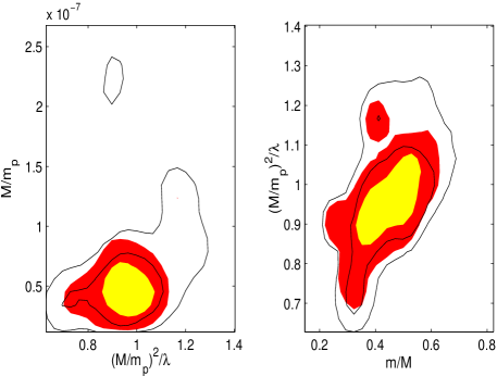
Figure 1: 2-dimensional likelihood constraints for the double inflationary parameters for the potential (7). We show $1\sigma$ and $2\sigma$ contour bounds from $\bar{\chi}^{2}$ data (shaded contours) and the contours which contain $68\%$ and $95\%$ of all the points in our MC chains (solid lines, see discussion in the text).

In Fig. 2 we plot the likelihood constraints for the initial values of the scalar fields. These are also constrained to lie in a narrow region in the range $1.1<\phi_{\rm in}/\phi_{c}<1.8$ and $2\times 10^{-3}<\chi_{\rm in}/\chi_{0}<8\times 10^{-3}$ (here $\chi_{0}\equiv M/\sqrt{\lambda}$). This means that initial values of $\phi$ close to $\phi=\phi_{c}$ are favoured. Since $m_{\chi}$ is much larger than $H$ for $\phi\gg\phi_{c}$, the field $\chi$ is strongly suppressed for the initial conditions $\phi_{\rm in}/\phi_{c}\gg 1$. This corresponds to the case in which the perturbations exhibit violent growth in the tachyonic region, thus effectively ruled out in our linear analysis. The initial value of $\chi$ affects the number of $e$-folds during the second stage of inflation ($=N_{\rm 2nd}$). We obtain smaller $N_{\rm 2nd}$ for larger $\chi_{\rm in}/\chi_{0}$. As we find in Fig. 3, the likely values for the number of $e$-folds is $50\lesssim N_{\rm 2nd}\lesssim 65$ which corresponds to initial conditions $\chi_{\rm in}/\chi_{0}$ of order $10^{-3}$–$10^{-2}$.

It is rather surprising that the likelihood contours of $N_{\rm 2nd}$ are clustered in the region with cosmologically relevant scales. In order to obtain this result we did not put any prior for the maximum values of the total number of $e$-folds. We found that it is difficult to satisfy the conditions of COBE normalization and suppressed isocurvature perturbations unless $N_{\rm 2nd}$ ranges in the region $50\lesssim N_{\rm 2nd}\lesssim 65$. This implies that double inflation has a rich and complex structure relative to single-field inflation.

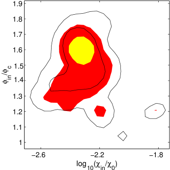
Figure 2: 2-dimensional likelihood constraints for the initial conditions of the field, $\{\phi_{\rm in}/\phi_{c},\chi_{\rm in}/\chi_{0}\}$.

Figure 3: Marginalised 1-d likelihood of the number of $e$-folds occurring during the 2nd phase of inflation. The solid line is based on the number of MCMC points, while the dotted line weighs each point based on its $\bar{\chi}^{2}$ value, as described in the caption to Fig. 1.

III.2 Power Spectrum

In this subsection we consider the contribution of isocurvature perturbations to the CMB anisotropies. In Fig. 4 we plot observational contour bounds for the amplitude ${\mathcal{P}}_{\cal R}$ and the two ratios ${\mathcal{P}}_{S}/{\mathcal{P}}_{\cal R}$, ${\mathcal{P}}_{C}/{\mathcal{P}}_{\cal R}$. The most likely value of ${\mathcal{P}}_{\cal R}$ is around ${\mathcal{P}}_{\cal R}=2.5\times 10^{-9}$, which is similar to the case of single-field inflation WM ; single .

The contribution of isocurvature perturbations is required to be small relative to adiabatic ones to be compatible with CMB anisotropies. As shown in Fig. 5 the TT spectrum in the isocurvature dominated case does not fit with the WMAP data at all. When isocurvature perturbations are comparable in magnitude to the adiabatic spectrum (labelled “mixed”), the spectrum shows significant deviations from the WMAP data on larger scales. We found the $2\sigma$ bounds: ${\mathcal{P}}_{S}/{\mathcal{P}}_{\cal R}<0.004$ and ${\mathcal{P}}_{C}/{\mathcal{P}}_{\cal R}<0.07$ in order to be consistent with WMAP.

In Fig. 6 we plot the observational contour bounds on $N_{\rm 2nd}$ and the spectral index $n_{s}$. There are some regions in which the spectrum of scalar perturbations is blue-tilted ($n_{s}>1$) with $N_{\rm 2nd}\lesssim 55$. Since the power spectra generated in the first and second stages of inflation are blue- and red-tilted respectively Tsuji , it is possible to have some suppression of power at low multipoles provided that the number of $e$-folds during the second stage of inflation satisfies $51\lesssim N_{\rm 2nd}\lesssim 55$. We show one example of the power spectrum in such a case in Fig. 5. Although strong suppression around $\ell=2,3$ is not easily achieved unless the spectrum is highly blue-tilted in this region (see e.g. Piao ), it is intriguing that this double inflation scenario provides a possibility to get a better fit on large scales.

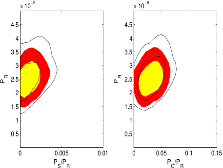
Figure 4: 2-dimensional likelihood contours for the amplitudes of the power spectra, with adiabatic against isocurvature (left) and adiabatic against correlated (right). Despite the freedom in allowing running of the spectra index the isocurvature component is severely constrained.

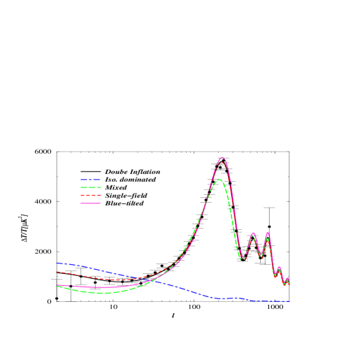
Figure 5: The CMB angular power spectra for five different cases:
(i) our best-fit double inflation model,
(ii) isocurvature dominating over the adiabatic,
 (iii) the isocurvature is comparable to the adiabatic (mixed),
(iv) the best fit single-field model with potential (12) and
(v) a model with blue-tilted spectrum ($n_{s}>1$) on large scales. The spectra are significantly different from the standard one when the isocurvature is dominant.

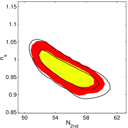
Figure 6: 2-dimensional likelihood contours for the spectral index $n_{s}$ and the number of $e$-folds during the second stage of inflation $N_{\rm 2nd}$.

IV Double inflation versus single-field inflation

A natural question is whether the extra complexity and fine-tuning involved in double inflation is actually preferred by the data over standard single-field inflation. This can be addressed by using the Akaike information criterion (AIC) and Bayesian Information criterion (BIC) bic . These two criteria are defined as:

$${\rm AIC} = -2\ln\,{\cal L}+2K\,,$$ (10)

$${\rm BIC} = -2\ln\,{\cal L}+K\ln\,N_{p}\,.$$ (11)

Here ${\cal L}$ is the maximum value of the likelihood, $K$ is the number of parameters and $N_{p}=1348$ is the number of WMAP data points. The optimal model minimises the AIC or BIC. In the limit of large $N_{p}$, AIC tends to favour models with more parameters while BIC more strongly penalises them (since the second term diverges in this limit). BIC provides an estimate of the posterior evidence of a model assuming no prior information. Hence BIC is a useful approximation to a full evidence calculation when we have no prior on the set of models (in this case single versus double inflation). In this case, we have no strong reason a priori to favour double inflation over single field inflation so BIC provides sensible approximation to a full evidence calculation.

Our double inflation model has 5 inflationary parameters ($M$, $m$, $\lambda$, $\phi_{\rm in}$, $\chi_{\rm in}$). We compare this with a single-field scenario with potential

$$V=\frac{\lambda}{4}\left(\chi^{2}-\frac{M^{2}}{\lambda}\right)^{2}\,.$$ (12)

This has 3 inflationary parameters ($\lambda$, $M$, $\chi_{\rm in}$). There are also 4 cosmological parameters, common to both models. In Table 1 we show the best-fit $\bar{\chi}^{2}$ and the values taken by the criteria for the models we have considered.

Model	$-2\ln\,{\cal L}$	AIC	BIC
Double inflation	1428.85	1446.85	1493.70
Single-field	1430.99	1444.99	1480.43

Table 1: The best-fit $\bar{\chi}^{2}$ ($=-2\ln\,{\cal L}$) and best Akaike and Bayesian Information criteria (AIC and BIC) for single and double inflation. Both criteria favour single field inflation.

We find that the best-fit value of $-2\ln\,{\cal L}$ in double inflation is smaller than in the case of single-field inflation. However both the AIC and BIC values for double inflation are significantly larger than those in the latter case, which suggests that single-field inflation is favoured relative to double inflation. In addition one could argue that single light-field inflation should theoretically be preferred a priori since it does not require fine-tuning to achieve more than one field to be light relative to the Hubble constant. Adding this prior will further favour single-field inflation.

We have only included WMAP data. Evidence for running of the spectral index from WMAP and lyman-$\alpha$ data run would favour double inflation models in which tilt is generic Tsuji . However evidence for running is currently weak recentrun and hence should not affect our conclusions significantly. Strong evidence for running in future data might change the situation however.

V Conclusions

In this paper we have studied observational constraints on double inflation using the WMAP first year data. The model we adopted is the supersymmetric hybrid potential given in Eq. (7). The presence of a tachyonic instability region after symmetry breaking leads to the correlation between adiabatic and isocurvature perturbations, which can significantly alter the CMB power spectrum compared to the case of adiabatic perturbations alone.

Comparing with first year WMAP CMB data we found that the correlated isocurvature component can be at most $7\%$ of the total contribution which is dominated by the adiabatic spectrum.

We carried out likelihood analysis in terms of 5 inflationary parameters and 4 cosmological parameters. The likelihood values of inflationary parameters are clustered in a narrow region around $M/m_{p}\sim 5.0\times 10^{-8}$, $\lambda\sim(M/m_{p})^{2}$ and $m/M\sim 0.5$ (see Fig. 1).

In spite of the large number of freedom of model parameters relative to single-field inflation, the parameter space of double inflation is severely constrained. This comes from the fact that it is not so easy to satisfy all constraints including COBE normalization and sufficiently suppressed isocurvature perturbations.

We also found that the number of $e$-folds in the second stage of inflation are constrained to lie in the range $50\lesssim N_{\rm 2nd}\lesssim 65$. Loss of power on large scales (relevant to achieving suppressed CMB low multipoles) is possible when the number of $e$-folds is around $51\lesssim N_{\rm 2nd}\lesssim 55$.

We also compared double inflation with single-field inflation by using the Akaike (AIC) and Bayesian information criteria (BIC). While the minimum value of $\bar{\chi}^{2}$ in double inflation is slightly smaller than in single-field inflation, the information criteria strongly support single-field inflation over the supersynmmetric hybrid double inflation models we studied.

Nevertheless we need to caution that the minimum $\bar{\chi}^{2}$ is still larger than the number of data points $N_{p}$ in current observations. We expect that future high-precision data such as the Planck satellite will provide more sophisticated information to distinguish between double inflation and single-field inflation.

In this regard it will be interesting to extend our analysis to include more fields, so that the matter power spectrum can exhibit sharp features, and to allow more realistic treatment of reheating. Both of these will increase the number of inflationary parameters (by about 2 or 3 each) and it is difficult to imagine them producing smaller values of the AIC and BIC as a result.

It seems likely therefore that single field inflation will continue to be the scenario to beat. It is intriguing that both the early and late universe seem well-described by very simple inflationary stages, and perhaps even two pure de Sitter phases. Finding a theoretical basis for this perplexing high-energy/low-energy duality may become a dominant quest in cosmology in the coming years.

References

- (1) T. D. Saini, J. Weller and S. L. Bridle, Mon. Not. Roy. Astron. Soc. 348, 603 (2004).
- (2) B. A. Bassett, P. S. Corasaniti and M. Kunz, arXiv:astro-ph/0407364.
- (3) J. Martin and C. Ringeval, Phys. Rev. D 69, 083515 (2004); P. Hunt and S. Sarkar, arXiv:astro-ph/0408138.
- (4) P. Mukherjee and Y. Wang, Astrophys. J. 599, 1 (2003); N. Kogo, M. Matsumiya, M. Sasaki and J. Yokoyama, Astrophys. J. 607, 32 (2004); D. Tocchini-Valentini, M. Douspis and J. Silk, arXiv:astro-ph/0402583; N. Kogo, M. Sasaki and J. Yokoyama, arXiv:astro-ph/0409052.
- (5) D. Polarski and A. A. Starobinsky, Phys. Rev. D 50, 6123 (1994).
- (6) A. A. Starobinsky and J. Yokoyama, arXiv:gr-qc/9502002.
- (7) J. Garcia-Bellido and D. Wands, Phys. Rev. D 53, 5437 (1996).
- (8) M. Sasaki and E. D. Stewart, Prog. Theor. Phys. 95, 71 (1996).
- (9) T. Chiba, N. Sugiyama and J. Yokoyama, Nucl. Phys. B 530, 304 (1998).
- (10) T. Kanazawa, M. Kawasaki, N. Sugiyama and T. Yanagida, Phys. Rev. D 61, 023517 (2000).
- (11) S. Tsujikawa and H. Yajima, Phys. Rev. D 62, 123512 (2000).
- (12) A. A. Starobinsky, S. Tsujikawa and J. Yokoyama, Nucl. Phys. B 610, 383 (2001).
- (13) J. c. Hwang and H. Noh, Class. Quant. Grav. 19, 527 (2002).
- (14) S. Tsujikawa and B. A. Bassett, Phys. Lett. B 536, 9 (2002).
- (15) S. Groot Nibbelink and B. J. W. van Tent, Class. Quant. Grav. 19, 613 (2002).
- (16) D. Langlois, Phys. Rev. D 59, 123512 (1999); D. Langlois and A. Riazuelo, Phys. Rev. D 62, 043504 (2000).
- (17) R. Trotta, A. Riazuelo and R. Durrer, Phys. Rev. Lett. 87, 231301 (2001).
- (18) C. Gordon, D. Wands, B. A. Bassett and R. Maartens, Phys. Rev. D 63, 023506 (2001).
- (19) N. Bartolo, S. Matarrese and A. Riotto, Phys. Rev. D 64, 123504 (2001).
- (20) D. Wands, N. Bartolo, S. Matarrese and A. Riotto, Phys. Rev. D 66, 043520 (2002).
- (21) S. Tsujikawa, D. Parkinson and B. A. Bassett, Phys. Rev. D 67, 083516 (2003).
- (22) F. Di Marco, F. Finelli and R. Brandenberger, Phys. Rev. D 67, 063512 (2003).
- (23) L. Amendola, C. Gordon, D. Wands and M. Sasaki, Phys. Rev. Lett. 88, 211302 (2002).
- (24) H. V. Peiris et al., Astrophys. J. Suppl. 148, 213 (2003).
- (25) M. Bucher, K. Moodley, N. Turok, Phys. Rev. D62, 083508 (2000); M. Bucher, K. Moodley, N. Turok, Phys. Rev. D66, 023528 (2002).
- (26) J. Valiviita and V. Muhonen, Phys. Rev. Lett. 91, 131302 (2003).
- (27) P. Crotty, J. Garcia-Bellido, J. Lesgourgues and A. Riazuelo, Phys. Rev. Lett. 91, 171301 (2003).
- (28) N. Bartolo, S. Matarrese and A. Riotto, Phys. Rev. D 65, 103505 (2002); F. Bernardeau and J. P. Uzan, Phys. Rev. D 66, 103506 (2002).
- (29) K. Moodley, M. Bucher, J. Dunkley, P. G. Ferreira and C. Skordis, arXiv:astro-ph/0407304.
- (30) A. Lewis and A. Challinor, Phys. Rev. D. 66, 023531 (2002).
- (31) M. Bucher, J. Dunkley, P. G. Ferreira, K. Moodley, C. Skordis, Phys. Rev. Lett. 93, 081301 (2004)
- (32) L. Verde et al., Astrophys. J. Suppl. 148, 195 (2003).
- (33) A. D. Linde, Phys. Rev. D 49, 748 (1994).
- (34) E. J. Copeland, A. R. Liddle, D. H. Lyth, E. D. Stewart and D. Wands, Phys. Rev. D 49, 6410 (1994).
- (35) L. Randall, M. Soljacic and A. H. Guth, Nucl. Phys. B 472, 377 (1996).
- (36) D. H. Lyth and A. Riotto, Phys. Rept. 314, 1 (1999).
- (37) J. Garcia-Bellido, A. D. Linde and D. Wands, Phys. Rev. D 54, 6040 (1996).
- (38) W. R. Gilks, S. Richardson & D. J. Spiegelhalter, Markov Chain Monte Carlo in practice, Chapman & Hall: London (1996).
- (39) A. Lewis and S. Bridle, Phys. Rev. D 66, 103511 (2002).
- (40) M. Tegmark et al., Phys. Rev. D 69, 103501 (2004).
- (41) V. Barger, H. S. Lee, and D. Marfatia, Phys. Lett. B 565, 33 (2003); W. H. Kinney, E. W. Kolb, A. Melchiorri and A. Riotto, Phys. Rev. D 69, 103516 (2004); S. M. Leach and A. R. Liddle, Phys. Rev. D 68, 123508 (2003); S. Tsujikawa and A. R. Liddle, JCAP 0403, 001 (2004); G. Calcagni and S. Tsujikawa, arXiv:astro-ph/0407543.
- (42) Y. S. Piao, S. Tsujikawa and X. Zhang, Class. Quant. Grav. 21, 4455 (2004).
- (43) H. Akaike, IEEE Trans. Auto. Control, 19, 716 (1974); G. Schwarz, Annals of Statistics, 5, 461 (1978); T. T. Takeuchi, Astrophys. Space Sci. 271, 213 (2000); A. Nakamichi and M. Morikawa, PhysicaA 341, 215 (2004); A. R. Liddle, arXiv:astro-ph/0401198.
- (44) D. N. Spergel et al., Astrophys. J. Suppl. 148, 175 (2003).
- (45) M. Viel, J. Weller and M. Haehnelt, arXiv:astro-ph/0407294.