Dynamical state and star formation properties of the merging galaxy cluster Abell 3921

We present the analysis and results of a new VRI photometric and spectroscopic survey of the central $\sim\leavevmode\nobreak\ 1.8{\times}1.2\leavevmode\nobreak\ {\rm Mpc}^{2}$ region of the galaxy cluster A3921 ($z=0.094$). We detect the presence of two dominant clumps of galaxies with a mass ratio of $\sim$5: a main cluster centred on the BCG (A3921-A), and a NW sub-cluster (A3921-B) hosting the second brightest cluster galaxy. The distorted morphology of the two sub-clusters suggests that they are interacting, while the velocity distribution of 104 confirmed cluster members does not reveal strong signatures of merging. By applying a two-body dynamical formalism to the two sub-clusters of A3921, and by comparing our optical results to the X-ray analysis of A3921 based on XMM observations (Belsole et al. 2004), we conclude that A3921-B is probably tangentially traversing the main cluster along a SW/NE direction. The two sub-clusters are observed in the central phase of their merging process ($\pm$ 0.3 Gyr), with a collision axis nearly perpendicular to the line of sight. Based on the spectral features of the galaxies belonging to A3921, we estimate the star formation properties of the confirmed cluster members. Substantial fractions of both emission-line ($\sim$13%) and post-star-forming objects (k+a’s, $\sim$16%) are detected, comparable to those measured at intermediate redshifts. Our analysis reveals a lack of bright post-star forming objects in A3921 with respect to higher redshift clusters, while the fraction of k+a’s increases towards fainter magnitudes ($M_{R_{\rm AB}}>-20$). Similar results were obtained in Coma cluster by Poggianti et al. 2004, but at still fainter magnitudes, suggesting that the maximum mass of actively star-forming galaxies increases with redshift (“downsizing effect”). The spatial and velocity distributions of k+a’s galaxies do not show significant differences to that of the passive population, and to the whole cluster. Most of these objects show relatively red colours and moderate Balmer absorption lines, which suggest star formation has ceased $\sim 1-1.5$ Gyr ago. Their presence is therefore difficult to relate to the on-going merging event. We find that star forming galaxies share neither the same kinematics, nor the same projected distribution of the passive cluster members. Moreover, most of emission-line galaxies are concentrated in A3921-B and in the region between the two sub-clusters. We therefore suggest that the ongoing merger may have triggered the star-formation episode in at least a fraction of the observed emission-line galaxies.

1 Introduction

In the standard cosmological scenario of hierarchical structure formation, bound objects form from the collapse of initial density fluctuations that grow under the influence of gravity through merging of smaller structures that have formed before. As optical and X-ray studies reveal that clusters of galaxies are still forming at the present epoch (e.g. Jones & Forman 1992, West et al. 1995, Donnelly et al. 2001), merging clusters provides a unique tool to test or analyze the physics of structure formation and evolution.

Major cluster–cluster collisions are the most energetic events that have occurred in the Universe since the Big Bang, as they release total energies up to $3\leavevmode\nobreak\ {\times}\leavevmode\nobreak\ 10^{64}$ erg (Sarazin 2003), and their effects on all cluster components are far from being fully understood. The intra-cluster gas experiences compression, rarefaction and shock waves (Schindler & Müller 1993), and shows characteristic features such as cold fronts (Markevitch et al. 2000). Additionally, on the side of the galaxy distribution, the velocity dispersion of the cluster members can increase up to a factor of two during the merger event (Schindler and Böhringer 1993). While the effects on the intra-cluster medium and on cluster internal dynamics have been analyzed in some details, the effects on the galaxies are still debated. Caldwell et al. (1993) showed that strong Balmer-line absorption galaxies are distributed between the main Coma cluster and the merging SW sub-cluster, suggesting star formation is triggered by the merging event. However, various physical mechanisms have been shown to affect the process of star formation within clusters. Changes of the tidal gravitational field during cluster merging could affect star formation in galaxies (e.g. Bekki 1999). The increasing external pressure following the infall of galaxies into the dense intra-cluster gas may trigger star formation (Dressler & Gunn 1983, Evrard 1991), while gas stripping in galaxies due to ram-pressure exerted by the ICM could weaken the starburst phenomenon during cluster–cluster collisions (Fujita et al. 1999). So far it is not clear which one of these competing effects is the dominant one, since results in favour of the former (e.g. Abraham et al. 1996, Wang, Ulmer & Lavery 1997, Moss & Whittle 2000, Flores et al. 2000, Gavazzi et al. 2003, Poggianti et al. 2004) and the latter (e.g. Tomita et al. 1996, Balogh et al. 1997, 1998, Baldi, Bardelli & Zucca 2001) were obtained.

Combined optical and X-ray studies have been particularly successful in revealing the complex dynamics of merging clusters (e.g. Davis et al. 1995, Lemonon et al. 1997, Roettiger et al. 1998, Durret et al. 1998, Arnaud et al. 2000, Donnelly et al. 2001, Ferrari et al. 2003). The X-ray properties of merging clusters are currently being investigated through a set of XMM observations (XMM guaranteed time, Sauvageot et al. 2001), together with the properties of their galaxy distribution through optical observations by our group, hence providing a unique combined analysis. In this paper we will concentrate on the optical analysis of the merging cluster Abell 3921, and our results will be compared to conclusions obtained from the X-ray analysis of XMM data by Belsole et al. 2004.

Abell 3921 is a R=2, BM II Abell cluster at $z=0.094$ (Katgert et al. 1998). Previous ROSAT and Ginga observations revealed the presence of a main cluster and a substructure with a very perturbed morphology, interpreted as falling onto the main component (Arnaud et al. 1996). Following XMM-Newton/EPIC observations (Sauvageot et al. 2001) confirmed the presence of a two component structure. This motivated new optical observations in order to better characterize the merger scenario of this complex cluster. In this paper, we analyze the spectroscopic and photometric galaxy catalogues of the central $\sim\leavevmode\nobreak\ 1.8{\times}1.2\leavevmode\nobreak\ {\rm Mpc}^{2}$ region of the cluster, with new data of multi-object spectroscopy (239 new spectra) and VRI-bands imaging, obtained with EFOSC2 at the 3.6m ESO telescope and with WFI at the 2.2m ESO telescope respectively. Sect. 2 briefly describes the observations, the data processing technique and the completeness level achieved by the new spectroscopic sample. In Sect. 3 cluster members are identified and in Sect. 4 the optical morphology of the cluster is studied. In Sect. 5 we perform a kinematical and dynamical analysis of the cluster. The optical masses of the two main subclusters are estimated in Sect. 6, and we solve the two-body problem for these two systems. The photometric and spectral properties of the cluster members are investigated in Sect. 7, allowing to define several subsamples whose spatial and velocity distributions are analyzed. The main results and their interpretation are summarized in the final Sect. 8. All numbers are expressed as a function of $h_{75}$, the Hubble constant in units of 75 km/s/Mpc. We have used the $\Lambda$CDM model with $\Omega_{m}=0.3$ and $\Omega_{\Lambda}=0.7$, then 1 arcmin corresponds to $\sim$0.097 ${{h}_{75}}^{-1}$ Mpc in the following.

2 The data

2.1 Imaging

The optical observations of Abell 3921 were carried out using the Wide Field Imager (WFI) mounted at the Cassegrain focus of the MPG/ESO 2.2m telescope at La Silla observatory. WFI is a mosaic camera with 4$\times$2 CCD chips covering a total area of 34$\times$33 arcmin². To cover the gaps between the eight individual chips of the camera we adopted a standard dithering sequence. The field centred on $\alpha=22^{h}49^{m}44^{s}$ $\delta=-64\hbox{${}^{\circ}$}22^{m}15^{s}$ was observed in service mode in the V,R and I passbands. The data, including photometric calibration images, were obtained between August 20th and 23rd, 2001. In Table 1, we summarize the observations.

Filter	ESO id	Nr. of Exp.	Total Exp.	Seeing	Mag.limit (AB)
			(s)	(arcsec)	(5$\sigma$,2$\times$FWHM)
V	V/89	5	750	1.35	22.5
R	Rc/162	5	750	1.15	22.7
I	Ic/Iwp	10	1800	1.25	21.5

Table 1: Imaging: summary of the observations

The data reduction was performed using the package ”alambic” developed by B.Vandame based on tools available from the multi-resolution visual model package (MVM) by Bijaoui and collaborators (Bijaoui & Rué 1995, Rué & Bijaoui 1997). The photometric calibration was obtained using several standard stars from Landolt (1992) over a large range of airmasses, leading to an accuracy of the photometry of $\sim 0.05$mag.

The SExtractor software package (Bertin & Arnouts 1996) was used to identify all sources in the field as well as to classify them and measure their magnitudes. The latter were corrected for galactic absorption using $E(B-V)=0.027$ as derived from Schlegel et al. (1998), yielding $A_{V}=0.09$mag, $A_{R}=0.07$mag and $A_{I}=0.05$mag. They were also transformed to the AB system given by the following relations: $V_{\rm AB}=V-0.01$, $R_{\rm AB}=R+0.19$, $I_{\rm AB}=I+0.49$.

2.2 Spectroscopy

In this paper we present the results of the analysis of new spectroscopic data obtained through two sessions of observations at the ESO 3.6 m telescope (2 nights in September 2001, 2 nights in October 2002). We used the ESO Faint Object and Camera (EFOSC2) with grism#03 and a punching head of 1.35”, obtaining a spectral resolution of FWHM$\sim$7.5 Å over the wavelength range 3050-6100 Å. For each frame we made at least two science exposures, in order to eliminate cosmic rays, with an integrated exposure time of 5400 s for brighter objects ($R_{\rm AB}<$18) and of 7200 s for fainter ones (${\rm R}_{\rm AB}<$19). We made a standard spectroscopic reduction using our automated package for multi–object spectroscopy based on the task “apall” in IRAF. Spectra were wavelength calibrated using the Helium–Argon lamp spectra taken after each science exposure. We determined redshifts using the cross–correlation technique (Tonry & Davis, 1981) implemented in the task “xcsao” of the RVSAO package. Spectra of late–type stars were used as radial velocity standards.

In Table 9 (available in the electronic version of the paper) we list the results of our spectroscopic observations in the following way: Col. 1: identification number of each target galaxy; Cols. 2 and 3: right ascension and declination (J2000.0) of the target galaxy; Cols. 4, 5 and 6: the V, R and I band magnitudes in the AB system; Cols. 7 and 8: best estimate of the heliocentric redshift (expressed as $cz$) and associated error from the cross-correlation technique (those values have been set to “-2” if the object is a star and to “-1” if we have no redshift information); Col. 9: run of observations; Col. 10: a quality flag for the redshift determination: 1=good determination (R parameter of Tonry & Davis $\geq$ 3), 2=uncertain determination, 3=no determination; Cols. 11 and 12: the equivalent widths (negative or positive in the case of emission or absorption features respectively) for [OII]$\lambda$3727 and ${\rm H}_{\delta}$ ($\lambda$=4101 Å) lines, measured only for the cluster members; Col. 13: the spectral classification of the galaxy members.

A total of 239 new spectra have been obtained, among which 56 are stars, 100 are galaxies with a very good redshift determination and 83 are spectra with $R<3$. In the following analysis, we also consider the redshifts measured in the region of A3921 by other authors (ENACS collaboration, Katgert et al. 1996, Mazure et al. 1996). We compare the values of the redshifts of 11 galaxies obtained from the common sample to those published (35) and we obtain a mean difference of -12.7$\pm$75.8 km/s, which shows a good consistency between the two datasets. The final sample includes our 239 redshifts and 24 available redshifts from the ENACS catalogue (Katgert et al. 1996, Mazure et al. 1996), among which 22 with quality flag=1 following our criterion. It covers a field of ${\sim}25.5^{\prime}{\times}25^{\prime}$, slightly larger than the size of our own spectroscopic follow-up (${\sim}18^{\prime}{\times}12.5^{\prime}$).

The $R$–band magnitude distribution of the whole spectroscopic sample of galaxies is presented in Fig. 1 (207 galaxies), and compared to the distribution of galaxies with a good redshift determination, i.e. quality flag=1 (122 galaxies), and among them, those belonging to A3921 (104 galaxies, see Sect. 3).

Figure 1: R-band magnitude distributions of the galaxies of our spectroscopic sample (207 objects - doted line), of all the galaxies with good velocity determination (122 - dashed line), and, among them, of those belonging to A3921 (104 - shaded area).

The ratio of the number of galaxies with measured redshift to the total number of galaxies detected within the central field of $18{\times}12.5\leavevmode\nobreak\ {\rm arcmin}^{2}$ covered by our last observations is plotted in Fig. 2 as a function of the $R$–band magnitude. The spectroscopic catalogue is complete at more than 50% level up to $R_{\rm AB}=18.5$ ($R_{\rm AB}^{*}$+2.1).

Figure 2: Completeness of the spectroscopic sample as a function of the R-band magnitude in the central $18{\times}12.5\leavevmode\nobreak\ {\rm arcmin}^{2}$ field for all galaxies observed (dashed line) and for those that led to a Quality Flag=1 (solid line).

Among the 263 objects of our spectroscopic sample, we will consider in the following only the 122 galaxies with redshifts determined with a quality flag=1 (i.e. our new 100 high quality spectra plus 22 published previously).

3 Cluster membership

Figure 3: Apparent radial velocity ($cz$) histogram of the galaxies in the central field of the cluster A3921, with a binning of 500 km/s.

Fig. 3 shows the radial velocity ($cz$) distribution of this dataset in bins of 500 km/s. The bulk of the cluster is concentrated between 25400 and 30400 km/s. Four objects have $cz$ higher than 75000, one galaxy appears to be in the foreground, while 13 are located between 31000 and 50000 km/s and most of them (12) are also spatially concentrated in the region around the two brightest objects of the West side of the cluster, BG2 and BG3. If we consider only the 8 galaxies around 40000 km/s, they correspond to a peak located at ${C}_{BI}=40378$ km/s ($\bar{z}=0.135$) with a velocity dispersion $S_{BI}=427$ km/s, indicating that they could be a background group.

In order to eliminate the galaxies not belonging to the cluster, we apply the standard iterative 3$\sigma$ clipping (Yahil & Vidal 1977). 104 cluster members with $cz$ between 25400 and 30400 km/s are selected. Note that the background peak being located $\sim$10000 km/s behind the mean velocity of the cluster is excluded as a subgroup of the cluster. Fig. 4 shows the location of the 104 identified members superimposed to a fraction of the R-band image.

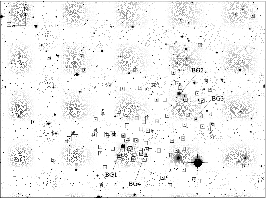
Figure 4: Galaxies identified as members of A3921 (squares), superimposed to a fraction of the R-band image (27’${\times}20^{\prime}$).

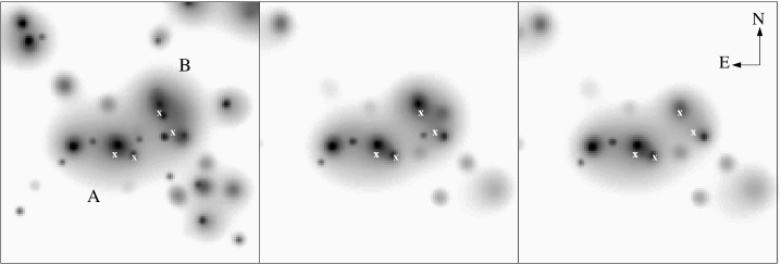
Figure 5: Projected galaxy density maps (with $R_{\rm AB}\leq 19$) on a 34${\times}34{\rm arcmin}^{2}$ field centred on A3921. Left panel: All galaxies; central panel: the red sequence galaxies, and right panel: same as central panel but removing galaxies known not to be cluster members from spectroscopy. The white crosses show the positions of the four brightest galaxies indicated in Fig. 4.

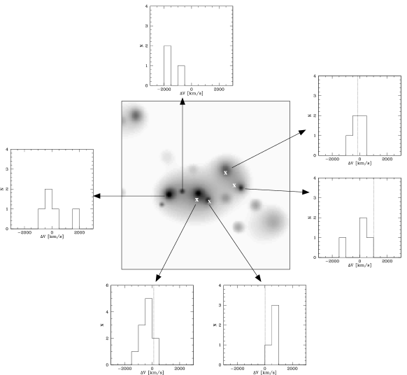
Figure 6: Velocity distributions of the main structures of the projected galaxy density map (same as the right panel of Fig. 5). The dotted line in the histogram indicate the relative velocity of the neighbouring brightest galaxy. At the level of $R_{\rm AB}=19$ all the selected clumps have a 100% coverage except the eastern group with 70% completeness.

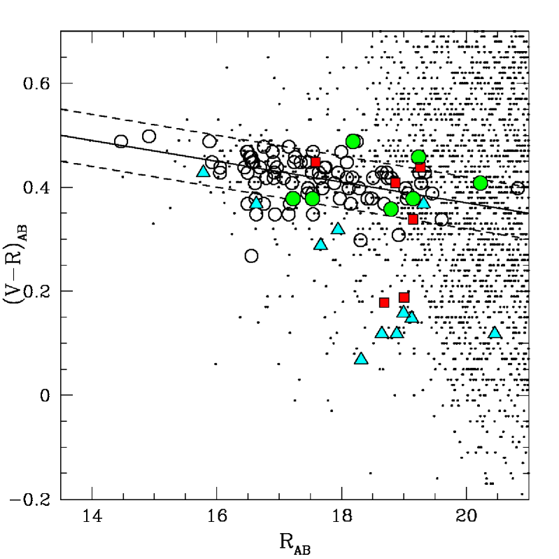
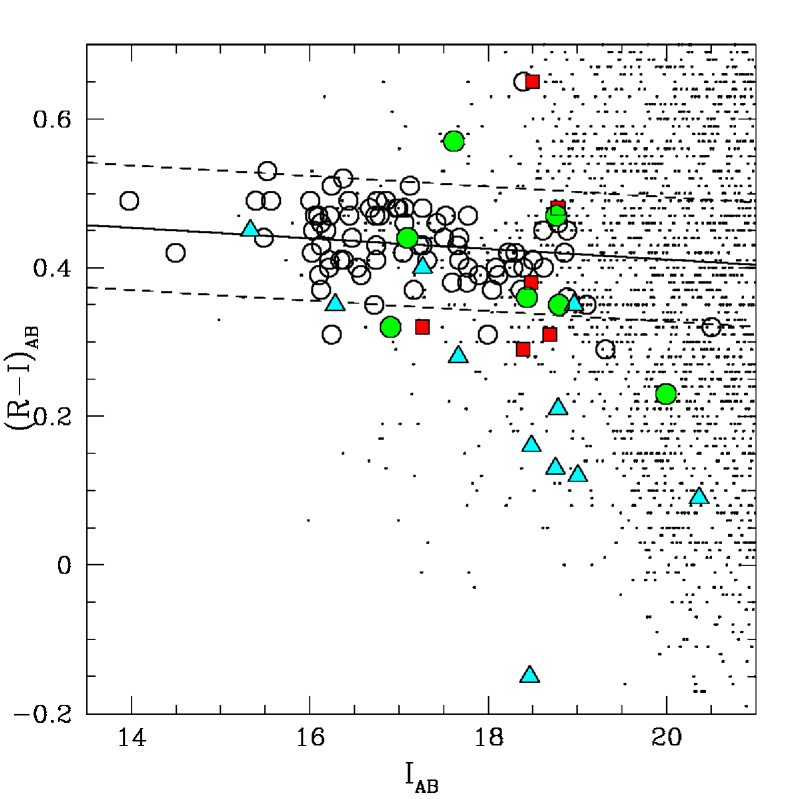
Figure 7: $(V-R)_{\rm AB}$ vs $R_{\rm AB}$ (left) and $(R-I)_{\rm AB}$ vs $I_{\rm AB}$ (right) colour-magnitude diagrams. All galaxies within 34$\times$34 ${\rm arcmin}^{2}$ are shown. Big symbols correspond to confirmed cluster members whereas dots correspond to galaxies without spectroscopic information. Triangles correspond to emission line galaxies, squares to k+a type, circles to galaxies presenting an H-K inversion following the classification described in the text. The solid line is the best linear-fit to the red sequence of the cluster, while the dotted line is at $\pm 1\sigma_{\rm RS}$.

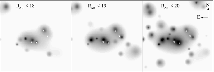
Figure 8: Projected galaxy density maps (using red sequence galaxies and excluding galaxies known not to be cluster members from spectroscopy, as in the right panel of Fig. 5) on a 34${\times}34{\rm arcmin}^{2}$ field centred on A3921 and for three magnitude cuts. The white crosses indicate the positions of the four brightest galaxies indicated in Fig. 4.

4 Colour properties and spatial morphology of A3921

In order to investigate the projected spatial morphology of A3921 several density maps of the galaxy distribution are built on the basis of a multi-scale approach. The adopted algorithm is a 2D generalization of the algorithm presented in Fadda et al. (1998). It involves a wavelet decomposition of the galaxy catalogue performed on five successive scales from which the significant structures are recombined into the final map (following the equation [C7] of Fadda et al. 1998). These significant structures are obtained by thresholding each wavelet plane at a level of three times the variance of the coefficients of each plane except for the two smallest scales for which the threshold is increased to four and five times the variance in order to reduce false detections due to the very low mean density of the Poisson process at these scales (0.01 for a chosen grid of 128$\times$128 ${\rm pixel}^{2}$).

Such density maps are presented in Fig. 5 for three input catalogues. In the left panel, all galaxies with $R_{\rm AB}<19$ (${\rm R}_{\rm AB}^{*}$+2.6) are used, leading to a map revealing two dominant clumps in the central part of the field (hereafter A3921-A in the centre and A3921-B to the NW) in the central $\sim$ 34$\times$34 ${\rm arcmin}^{2}$. In order to avoid possible projection effects, we isolate galaxies likely to be early-types at the same redshift on the basis of their colour properties. Indeed, despite the bimodal structure of A3921 one can notice in the two colour magnitude diagrams of Fig. 7 a well defined red sequence, the characteristic linear structure defined by the bulk of early-type galaxies in a cluster. The determination of the slope, intercept and width of these ”red sequences” is performed using the technique described in Appendix A. The central panel of Fig. 5 shows the resulting red sequence density map (keeping only galaxies at $\pm 1\sigma$ around the red-sequence), where one can notice that several small-scale clumps in the cluster core disappear as well as in its surroundings, leaving the larger-scale structure of the two main clumps unaffected.

In order to go one step further in avoiding projection effects we take advantage of our spectroscopic follow up. Even if it is complete down to a level of 50% at $R_{\rm AB}=19$, most of the clumps seen visually have been spectroscopically sampled allowing us to discard possible external groups. For example, as mentioned in the previous section, the background redshift-peak group may lead to an over-density unrelated to the cluster in the iso-density map. Therefore, from the sample of red sequence galaxies we additionally exclude galaxies known from spectroscopy not to be cluster members. The result is shown in the right panel of Fig. 5, which is quite similar to the map in the central panel except that the location of clump B is shifted towards South and its central peak is shifted close to the position of the BG2. If we can trust in the high confidence level that the sub-structures still visible are part of A3921, it is still not clear whether or not they are projection effects within the cluster. In Fig. 6 the relative velocity distributions of these various sub-structures are presented using the available redshifts. At the level of ${\rm R}_{\rm AB}=19$ these clumps actually have full spectroscopic coverage except for the eastern group with 5 confirmed cluster members out of 7 galaxies belonging to the red sequence. The strong clustering in redshift space for all the sub-structures confirms the accuracy of the picture reflected by this density map.

In Fig. 8 the same maps are presented for three magnitude cuts. The global bi-modal structure of the cluster remains unchanged with luminosity. This is particularly true for the central parts of clumps A and B. However, note that the eastern group, more compact than the clump B, is stronger at fainter levels.

The results given above are based on the only red sequence galaxies. In Fig. 9 the galaxies bluer than the red sequence are presented, superimposed on the red sequence iso-density map. These blue galaxies appear much less clustered than the redder ones over the whole field and show only little correlation with the red density peaks except in the case of clump B showing an excess of blue galaxies relative to the other clumps and in particular to the center of the clump A. This asymmetry is also present in the distribution of emission line galaxies as it will be shown and discussed in Sect. 7.3.1.

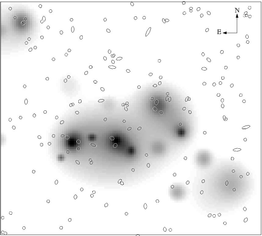
Figure 9: Projected galaxy density map (34$\times$34 ${\rm arcmin}^{2}$) of the red-sequence galaxies (see Fig.6). The symbols represent the galaxies with $R_{\rm AB}<20$ and bluer than the red sequence galaxies.

To summarize, A3921 is characterized by a) a bimodal morphology, b) the presence of several substructures inside each of the two main clumps, c) an offset of the BCG from the main density peak of clump A, and d) an excess of blue galaxies around the clump B. These results suggest that this system is out of dynamical equilibrium and that it is probably composed of a main cluster interacting with at least two groups, one to the North-East (clump B) and one to the East, the latter being significantly less luminous than the former. In the following section, we will analyze the dynamical properties of A3921 in order to understand which phase of the merging process we are witnessing.

5 Cluster Kinematics

5.1 Velocity distribution of the whole cluster

Using the biweight estimators for location and scale (Beers et al. 1990), we find a mean apparent velocity of $C_{BI}=28047^{+76}_{-77}$ km/s, corresponding to a mean redshift of $\bar{z}{\simeq}0.0936$, and a velocity dispersion of $S_{BI}=831^{+100}_{-76}$ km/s (at $1\sigma$ significance level, see Table 2). Fig. 10 shows the histogram of the cosmologically and relativistically corrected velocity offsets from the mean cluster redshift ($\Delta{v}=c(z-\bar{z})/(1+\bar{z})$) of the 104 cluster members. Contrary to the projected morphology on the sky we do not find any bi-modal structure in the velocity distribution. In dissipationless systems, gravitational interactions of cluster galaxies over a relaxation time generate a Gaussian distribution of their radial velocities; possible deviations from Gaussianity could provide important indications of ongoing dynamical processes. In the following, we are therefore interested in measuring a possible departure of the observed cluster velocity distribution from a Gaussian.

Subsample	$N_{gal}$	${C}_{BI}$	${S}_{BI}$	Skewness	AI	Kurtosis	TI
		[km/s]	[km/s]	%	%	%	%
Whole sample	104	$28047^{+76}_{-77}$	$831^{+100}_{-76}$	$\geq$10	$>$20	$\leq$10	$\leq$1
A3921-A	41	$28017^{+145}_{-173}$	$1008^{+156}_{-106}$	$>$10	$>$20	$>$20	$>$20
A3921-B	20	$27920^{+88}_{-86}$	$451^{+215}_{-80}$	$<$10	$<$5	$>$20	$>$10

Table 2: Properties of the $cz$ distribution and significance levels of shape estimators for various subsamples of A3921. ${C}_{BI}$ and ${S}_{BI}$ are the mean velocity and the velocity dispersion of the different distributions (biweight estimators for location and scale, Beers et al. 1990)

Figure 10: Top: Stripe density plot of the radial velocity offsets of the 104 A3921 members from $\bar{z}$ (corrected for cosmological and relativistic effects). The position of the gap detected in the cluster velocity distribution is indicated by an arrow. Bottom: Velocity histogram of the confirmed cluster galaxies in bins of 200 km/s. The Gaussian best–fit to the velocity distribution is superimposed.

A light–tailed velocity distribution can indicate the presence of two or more overlapping Gaussian components in the whole velocity histogram, while an asymmetric distribution can be the result of the contemporary presence of subclusters with different numbers of galaxies (Ashman et al. 1994). We use two kinds of shape estimators: the traditional third and fourth moments, i.e. skewness and kurtosis, and the asymmetry and tail indices (Bird & Beers, 1993). In Table 2 we report the corresponding values and significance levels, estimated from Table 2 in Bird & Beers 1993 under the null hypothesis of a Gaussian distribution.

The values obtained for Skewness and AI show that the velocity histogram is quite symmetric (significance level $>$10%). Values observed for kurtosis and TI indicate a heavy–tailed distribution, rejecting the Gaussian hypothesis at $\sim$10% significance level the first, even better than 1% the second. While light-tailed distributions indicate multi-modality, heavy populated tails could be due to contamination by non-cluster galaxies. We think that the analysis of Sect. 3 excludes this possibility, but we apply an additional test in order to definitively reject the presence of outliers in our velocity sample of 104 galaxies. Extensive data available for low-$z$ clusters show that most ($\geq$95%) of the galaxies in the central region of the clusters have radial velocities within $\pm$3500 km/s of the mean cluster redshift (Postman et al. 1998). We thus verify that all the 104 galaxies of our final sample have $|\Delta{v}|<$3500 km/s (with $\Delta{v}$ defined at the beginning of this section). In any case, the shape parameters do not show strong evidence of subcomponents in velocity space.

7 of the 13 normality tests performed by ROSTAT reject the Gaussian hypothesis at better than 10% significance level (see Table 3). Moreover, we find one significant weighted gap in our dataset (Beers et al. 1990) at $cz=27381.9$ km/s (shown in Fig. 10) and characterized by a normalized size of 2.47 and a significance of 3%. On the contrary, among the 6 tests performed by ROSTAT that do not reject the Gaussian hypothesis, the DIP test (Hartigan & Hartigan 1985) accepts the unimodal hypothesis at better than 99% level, in agreement with the conclusions obtained with the symmetry tests (i.e. Skewness and AI).

Classical tests of Gaussianity give therefore controversial results about the kinematical properties of A3921.

	Whole cluster
Statistical Test	Value	Significance
A	0.735	$<$1%
B2	3.567	8.8%
I	1.099	$<$5%
KS	0.901	5.0%
V	1.621	2.5 %
${\rm W}^{2}$	0.163	1.6%
${\rm U}^{2}$	0.159	1.2%
${\rm A}^{2}$	0.907	2.1%
	A3921-A
Statistical Test	Value	Significance
None	-	-
	A3921-B
Statistical Test	Value	Significance
A	0.684	$<5\%$
U	4.822	$\sim$1%
B1	-0.657	7.8%
B2	4.738	2.1%
B1 & B2	6.123	4.7%

Table 3: 1-D statistical tests performed in ROSTAT package that exclude the hypothesis of a single Gaussian distribution for the different velocity datasets considered in the paper. In Cols. 1 and 2 we report the name and the value of the statistics, while Col. 3 indicate their significance levels.

5.2 Analysis of a possible partition in redshift space and kinematical indicators of subclustering

Figure 11: Profile of the velocity means (top) and dispersions (bottom) in the cluster: left: as a cumulative function of galaxies centred on BG1 position - right: differential values as a function of radius in rings with 13 galaxies; the last point is far from the others due to the lower degree of completeness reached by spectroscopic data in the external regions of the cluster (out of the central $\sim$12’).

Due to the uncertain results obtained in previous section, we apply the KMM mixture-modeling algorithm of McLachlan & Basford (1988) which, using a maximum-likelihood technique, assigns each galaxy to a possible parent population, and evaluates the improvement in fitting a multiple–component model over a single–one. First of all, we try to allocate the 104 galaxies of our dataset into two possible subclusters, respectively with mean velocity lower and higher than the gap position. Several tests are then performed by changing both the estimated mean velocities and the estimated mixing proportion for each group, but we always obtain the same result: the KMM algorithm tries to fit a 2–group partition from these guesses, obtaining intermediate confidence levels that cannot reject the null hypothesis of unimodal distribution. This result actually agrees both with the DIP test and with what is observed from the shape parameters of the velocity distribution, the absence of light–populated tails and of a significant asymmetry in the histogram excluding the possible presence of several overlapping subunits populated differently.

Classical statistical tests for sub–clustering are then applied to the 104 cluster members in order to look for the existence of correlated substructures in velocity and spatial distributions (Dressler & Shectman, 1988; Bird, 1994; West & Bothun, 1990). The results, obtained by the bootstrap technique and 1000 Monte Carlo models, are presented in Table 4.

Indicator	Value	Significance
$\Delta$	109.284	0.680
$\epsilon$	${0.991}{\times}{10}^{+27}\leavevmode\nobreak\ {\rm kg}$	0.353
$\alpha$	0.129 ${{h}_{75}}^{-1}$ Mpc	0.914

Table 4: 3-D substructure indicators for the sample of 104 objects with quality flag=1 in the velocity range 25400$\div$30400 km/s

Both $\Delta$ and $\alpha$ parameters do not find evidence of substructures with a high significance level, while $\epsilon$ test has an intermediate and not conclusive value. Fig. 12 shows graphically the results obtained with the $\Delta$ test.

Figure 12: Projected positions, centred on BG1 coordinates, of the galaxies with $v_{r}=25400{\div}30400$. Each galaxy is represented by a circle, whose dimension is weighted by the estimator of Dressler & Shectman (1988). Filled circles (red in the electronic version of the paper) are centred on the three BGs positions.

In conclusion, while no bi-modality is shown in the velocity distribution, the various tests of gaussianity and subclustering do not reach a consensus, but do not show ”extreme” departures from gaussianity.

5.3 Radial profile of the velocity dispersion

The analysis of the mean velocity and particularly of the radial profile of the velocity dispersion provides a useful tool for investigating the dynamics of galaxy clusters, as they can reveal signs of subclustering and ongoing merging (Quintana et al. 1996, Muriel et al. 2002). Such integrated measurements are therefore performed with the 104 members of A3921 up to a distance of $\sim$ 2 ${{h}_{75}}^{-1}$ Mpc from the cluster centre (taken to be at the position of BG1), and are presented in the left panels of Fig. 11. The mean velocity has a very constant value ($\sim$28000 km/s) from the centre of the cluster to its outer edges. Following the classification of the radial profiles of the velocity dispersions of den Hartog & Katgert (1996), A3921 presents an ”inverted” shape: the cumulative velocity dispersion shows an initial increase with radius up to $\sim$4 arcmin apart from the cluster centre and then decreases nearly to its first bin value ($\sim$900 km/s). Finally, the velocity dispersion becomes flat in the external regions of the cluster ($\geq$1 ${{h}_{75}}^{-1}$ Mpc). This result suggests that this final value is representative of the total kinetic energy of the cluster members (Fadda et al. 1996). A similar shape was detected by den Hartog & Katgert (1996) and Nikogossyan et al. (1999) in the case of the galaxy cluster A194, and these authors interpreted such a profile as originated in a nearly relaxed region. Therefore, both the integrated radial profiles of the velocity dispersion and of the mean velocity do not reveal the presence of significant velocity gradients that could be produced by the presence of internal sub-structures. These results are confirmed by the right panels of Fig. 11, where mean velocities and velocity dispersions are estimated in rings containing the same number of galaxies (13). The shapes of these differential profiles agree with the integrated ones, presenting again an inverted shape. Its minimum velocity dispersion corresponds to the ring containing the group of galaxies located around BG2. Within error bars, mean velocities are nearly constant around 28000 km/s, as for the integrated profile.

5.4 Velocity distributions of A3921-A and A3921-B

Figure 13: Completeness of the spectroscopic sample for the two clumps A3921-A (solid line) and in A3921-B (dashed line).

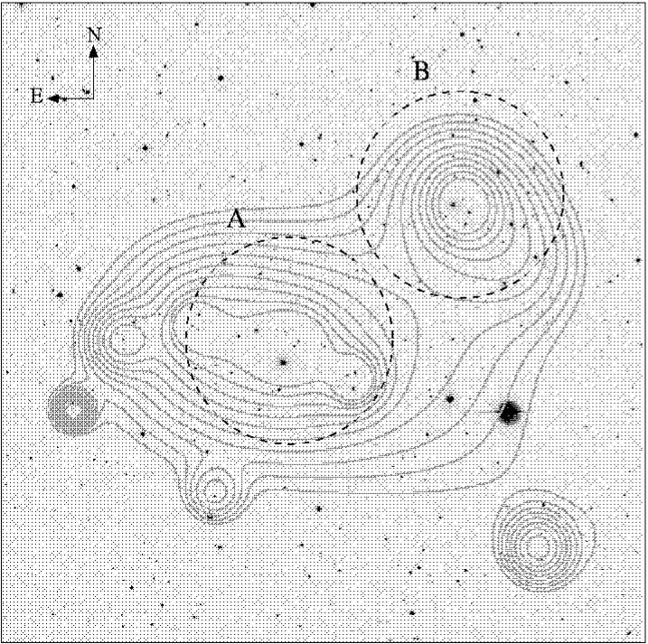
Figure 14: Iso-density contours of the projected distribution of the red-sequence galaxies (with $R_{\rm AB}\leq 18$ and after removing galaxies known not to be cluster members from spectroscopic data) superimposed to the central 22$\times$22 ${\rm arcmin}^{2}$ of the R–band image of A3921. The dynamical analysis of the two clumps A and B is performed based on the galaxies selected inside the two dashed circles (R$\simeq$ 0.34 Mpc).

As shown above, the dynamical and kinematical properties of the whole cluster do not reveal strong signatures of merging. More indications on the dynamical state of the cluster could come from the analysis of the velocity distribution of the two main subclusters detected on the iso-density maps separately. For this, our velocity sample is divided into two datasets, containing the confirmed cluster members in the two circles displayed in Fig. 14, chosen as the largest without intersecting. The radius of the two circles is $\simeq$ 0.34 Mpc and they are centred on the density peaks previously detected (Sect. 4). We plot in Fig. 13 the ratio of the number of galaxies with very good redshift determination (Q.F.=1) to the total number of objects detected in the two circles of Fig. 14 as a function of $R$–band magnitude; the spectroscopic sampling of these two regions, and in particular of A3921-A, appears quite good, with completeness levels $\geq$50% for $R_{\rm AB}\leq$19.5 ($\simeq R_{\rm AB}^{*}$+3.1).

Fig. 15 shows the velocity distributions of the two datasets and in Table 2 we quote their velocity means and dispersions. Both datasets show a velocity location very close to each other and to the whole cluster value (the velocity offset $\Delta{v}$ between A3921-A and A3921-B mean velocities is of only $89^{+155}_{-177}$ km/s); the clump A is characterized by the highest velocity dispersion.

Most (8) of the 13 normality tests contained in ROSTAT package accept the hypothesis of Gaussianity for the velocity distribution of the A3921-B component, and actually all of them do not reject the null hypothesis for the radial velocities of the clump A3921-A (Table 3). Shape parameters (Table 2) accept the Gaussian hypothesis at more than 10% significance level, with the exception of the skewness and of the kurtosis, that indicates the possible presence of an asymmetric velocity distribution (significance level lower than 10%) and of heavy populated tails (significance level lower than 5%) in the A3921-B velocity histogram.

Summarizing, Gaussianity tests suggest that the merging event has not strongly affected the internal dynamics of the two sub-clusters.

Figure 15: Velocity histogram, with a binning of 200 km/s, of the galaxies in A3921-A (solid line) and in A3921-B (dotted line), according to the division showed in Fig. 14. The relative Gaussian best–fits to the velocity distributions are superimposed. Arrows show the radial velocities of the three brightest cluster galaxies.

6 Dynamical study of the system

6.1 Mass estimate of the two main clumps

Determining the respective masses of A3921-A and A3921-B requires idealized assumptions which cannot be strictly valid for an interacting system. However, as seen in section  5.4, the dynamics of the central regions of the two clumps appears to be relatively unaffected by the merging event.

We have therefore assumed that each subcluster is virialized. As in the case of velocity dispersions, the virial radius of each clump was estimated selecting only those galaxies within a projected distance of $\sim$ 0.34 ${{h}_{75}}^{-1}$  Mpc from its center (see Fig. 14). In order to have a better statistics and at the same time to minimize biases due to spectral incompleteness and background contamination, we included all the galaxies belonging to the red sequence (thus assuming that early–type galaxies trace the mass profile; see Katgert, Biviano & Mazure 2004), except for those with a measured redshift and identified as outliers on the basis of our previous analysis.

The mass was calculated with the classical virial equation:

$$M_{vir}=\frac{r_{vir}\sigma_{vir}^{2}}{G}$$ (1)

where $\sigma_{vir}$ is the three–dimensional velocity dispersion of the system, and $r_{vir}$ is the virial radius:

$$r_{vir}\equiv-\frac{GM_{vir}^{2}}{U}=N^{2}\left(\sum_{i<j}^{N-1}\sum_{j=i+1}^{N}\frac{1}{r_{ij}}\right)^{-1}=\frac{2N}{N-1}r_{h}$$ (2)

In equation (2) $U$ is the potential energy of the system and $r_{h}$ is the mean harmonic radius, defined as:

$$r_{h}=\frac{N(N-1)}{2}\left(\sum_{i<j}^{N-1}\sum_{j=i+1}^{N}\frac{1}{r_{ij}}\right)^{-1}$$ (3)

where $r_{ij}$ is the separation between the $i$th and $j$th galaxies, and $N$ is the total number of objects in the system).

We have to apply the above relations to projected separations, so that we can estimate the projected mean harmonic radius $R_{H}$ and obtain the corresponding projected virial radius $R_{vir}$. Assuming spherical symmetry, $r_{vir}=(\pi/2)R_{vir}$ (see Limber & Mathews 1960) and $\sigma_{vir}=3\sigma_{r}$, where $\sigma_{r}$ is the radial velocity dispersion of the system.

The above method is based on the pairwise estimator of the harmonic radius: an alternative is the so–called ringwise estimator (see Carlberg et al. 1996). We have applied both methods, finding no significant difference (notice that this is not true in general).

$R_{vir}$ (A)	$R_{vir}$ (B)	$M_{vir}$ (A)	$M_{vir}$ (B)	$M_{vir}$ (A) / $M_{vir}$ (B)
0.39$\pm$0.02	0.38$\pm$0.02	$4.3^{+1.4}_{-1.0}$	$0.8^{+0.7}_{-0.3}$	$5.2^{+4.4}_{-2.5}$

Table 5: Columns 1 & 2: projected virial radii of A3921-A and A3921-B; columns 3 & 4: virial mass estimates for A3921-A and A3921-B; column 5: mass ratio. Masses are in $10^{14}{M}_{\odot}$ units and radiii in $h^{-1}$ Mpc units.

The results obtained applying the pairwise method along with the corresponding 1$\sigma$ errors, are shown in Table 5. The values of the virial radii are relatively small (only slightly larger than the window radius): we have to take into account the the possibility that they are underestimated, although they could be appropriate for subcluster systems.

Given our cosmology with $\Omega_{M}+\Omega_{\Lambda}=1$, we would expect $\bar{\rho}(r_{vir})\sim 100\rho_{c}$ (see e.g. Eke et al. 1996), where $\bar{\rho}(r_{vir})$ is the mean density within $r_{vir}$ and $\rho_{c}$ is the critical density. The ratio between these two quantities is related to the virial radius according to the following equation (always derived for our flat cosmology):

$$\frac{\bar{\rho}(r_{vir})}{\rho_{c}(z)}=\frac{1}{\rho_{c}(z)}\frac{3M_{vir}}{4\pi r_{vir}^{3}}=\frac{\sigma_{r}^{2}}{r_{vir}^{2}}\frac{6}{H_{0}^{2}[\Omega_{M}(1+z)^{3}+\Omega_{\Lambda}]}$$ (4)

Putting into the above equation the mean cluster redshift and the estimated values of the three-dimensional virial radii, $r_{vir}=\pi R_{vir}/2$, we find $\bar{\rho}(r_{vir})$ $\sim 2670\rho_{c}$ and $\sim 560\rho_{c}$ respectively for A3921-A and A3921-B, which indicates that we are probably underestimating the virial radii. A further uncertainty is associated to the surface pressure term, which acts in the opposite direction with respect to the previous correction for the underestimate of the virial radius (Carlberg et al. 1996 and references therein). However, while the exact values of the virial masses might be larger, it is clear that A3921 is made up by two unequal mass systems, with $M_{A}/M_{B}\sim 5$, a value which essentially reflects the factor 2 ratio between the velocity dispersion of the two clumps.

6.2 Two-body dynamical model

In this section, we apply the two-body dynamical formalism (Gregory and Thomson 1984, Beers et al. 1992) to the two sub-clusters of A3921. By assuming that at $t$=0 the two subclusters were at zero separation, parametric solutions to the equations of motion can be derived both in the bound:

$$R = \frac{R_{m}}{2}\leavevmode\nobreak\ (1-{\rm cos}{\chi})$$ (5)

$$t = \left(\frac{{R_{m}}^{3}}{8GM}\right)^{1/2}\leavevmode\nobreak\ (\chi-{\rm sin}{\chi})$$ (6)

$$V = \left(\frac{2GM}{R_{m}}\right)^{1/2}\leavevmode\nobreak\ \frac{{\rm sin}{\chi}}{1-{\rm cos}{\chi}},$$ (7)

and in the unbound case:

$$R = \frac{GM}{{V_{\infty}}^{2}}\leavevmode\nobreak\ ({\rm cosh}{\chi}-1)$$ (8)

$$t = \frac{GM}{{V_{\infty}}^{3}}\leavevmode\nobreak\ ({\rm sinh}{\chi}-\chi)$$ (9)

$$V = V_{\infty}\leavevmode\nobreak\ \frac{{\rm sinh}{\chi}}{{\rm cosh}{\chi}-1},$$ (10)

where $R_{m}$ is the separation of the two subclusters at maximum expansion, $M$ is the total mass of the system, $\chi$ is the developmental angle and $V_{\infty}$ is the asymptotic expansion velocity. The relative velocity $V$ and the spatial separation $R$ between the substructures are respectively related to their radial ($\Delta{v}$) and projected components ($R_{p}$) through the following relations:

$$V=\Delta{v}/{\rm sin}{\alpha};\leavevmode\nobreak\ \leavevmode\nobreak\ \leavevmode\nobreak\ R=R_{p}/{\rm cos}{\alpha}$$

where $\alpha$ is the angle between the plane of the sky and the line connecting the centres of the two clumps.

We close the system of equations taking our measured values of $R_{p}{\simeq}$0.74 Mpc and $\Delta{v}$=89 km/s, and assuming different values for $t_{0}$, i.e. the epoch of the last encounter between the two clumps (Gregory & Thompson 1984 and Barrena et al. 2002). This implies in each case a relationship between the total mass of the system $M$ and the angle $\alpha$ which is displayed in Fig.16.

In the first case, we set $t_{0}=12.6$ Gyr, i.e. the age of the Universe in our cosmology. This suggests that subclusters are moving apart or together for the first time. We are then in the pre-merger scenario. In the case of A3921, the measured total mass of the two sub-clusters is $M=5.2^{+1.6}_{-0.1}{\times}10^{14}\leavevmode\nobreak\ h_{75}^{-1}\leavevmode\nobreak\ {M}_{\odot}$ (Sect. 6.1). The top, left panel of Fig. 16 shows that the possible solutions for this value are bound. In the incoming case, two solutions are possible, with respectively a very high and a very low value for the projection angle $\alpha$, while in the outgoing case only a high value of $\alpha$ is allowed (cases (a) Table 6).

We then suppose we are witnessing the sub-clusters after the collision, testing the possible solutions for $t_{0}=$0.3 Gyr (case (b)), 0.5 Gyr(case (c)), and 1 Gyr (cases (d)). In all the cases, the possible solutions are bound as shown in Fig. 16 (top, right and bottom panels). For both the smaller values of $t_{0}$ (0.3 and 0.5 Gyr), there is only one outgoing solution possible, leading to increasing values of $\alpha$ for higher $t_{0}$ (see Table 6). At larger times after merging ($t_{0}=1$ Gyr), three values of $\alpha$ are possible, two for incoming solutions and one in the outgoing configuration (see Table 6). At this stage, apart from the fact that the sub-clusters are bound with a very high probability, it is difficult to discriminate between the various merging scenarios from the dynamical analysis of the galaxies alone.

Scenario	${\rm T}_{0}$	$\alpha$	V	R	Solutions
	[Gyr]	[deg]	[km/s]	[Mpc]
a1	12.6	84.3	89.4	7.5	outgoing
a2	12.6	83.5	89.6	6.5	incoming
a3	12.6	2.2	2318.4	0.7	incoming
b	0.3	4.9	1041.9	0.7	outgoing
c	0.5	27.8	190.8	0.8	outgoing
d1	1.0	55.2	108.4	1.3	outgoing
d2	1.0	50.6	115.2	1.2	incoming
d3	1.0	4.7	1086.2	0.7	incoming

Table 6: Col.1: name of the scenario in the text – Col.2: time since last interaction between the two clumps – Col.3: angle between the plane of the sky and the line connecting the centres of the two clumps – Col.4: relative velocity between the two clumps – Col.5: spatial separation between the two systems – Col.6: state of the systems for the possible solutions

Figure 16: The total mass of the two clumps as a function of the angle $\alpha$ between the plane of the sky and the line connecting the centres of the two sub-clusters. The horizontal solid line represents the sum of the pairwise projected masses as estimated in section 6.1; the associated 1$\sigma$ confidence level domain is limited by the two dot-dashed lines. Top left (cases a1, a2, a3 in Table 6): the solid line shows the bound-incoming and -outgoing solutions, while the dashed line corresponds to the unbound solutions. These solutions have been estimated under the hypothesis that the two systems were at zero separation 12.6 Gyr ago (i.e. the age of the Universe in our cosmology). Top right (case b): the same but assuming that the two systems were at zero separation 0.3 Gyr ago. The only possible configuration shows that the two clumps are bound and the system is expanding. Bottom (cases c and d1, d2, d3): same as in the top right panel, but by assuming that the collision took place 0.5 (left) and 1.0 (right) Gyr ago respectively.

7 Spectral properties of the cluster members

7.1 Measurements of the equivalent widths

In the following, we wish to assess the star formation properties of the galaxies belonging to A3921, and in particular to identify galaxies with signatures of recent star activity from an older population, as well as galaxies with emission lines, reflecting present star formation. This analysis is based on our high S/N spectra catalog, therefore restricted to 83 A3921 members. To reach this goal, the first step is to classify objects of our spectroscopic catalog of galaxies. Various methods have been used in the literature, using generally the presence and strength of the [OII] ($\lambda$=3727 Å) line and of Balmer lines (typically one or a combination of ${\rm H}_{\delta}$, ${\rm H}_{\gamma}$, and ${\rm H}_{\beta}$ lines). In principle, as shown by Newberry et al. 1990, the most robust approach to detect post-starburst galaxies would make full use of all three Balmer lines. However, our limited spectral range does not allow us to include ${\rm H}_{\beta}$ in numerous cases, and the S/N ratio of the ${\rm H}_{\gamma}$ line is generally poor. Therefore, we use the combination of [OII] and of the ${\rm H}_{\delta}$ line to establish our spectral classification, as in Dressler et al. (1999).

We apply two methods for measuring the equivalent widths of these lines, using respectively the tasks “splot” and “sbands” in IRAF on our continuum normalized spectra. The continuum is fitted by a spline function of high order (generally 9), and the quality of the best fit verified for each spectrum. In particular, special attention is paid to the good quality of the fit in the vicinity of the line to measure, which is crucial for a reliable measurement of the EW. While “splot” fits a gaussian for the line, “sbands” measures the decrement or increment in signal relative to the fitted continuum in an interval containing the line to be measured. We check the consistency of the measures with the two methods, and choose the Gaussian fitting technique because it gives more accurate measurements for the following analysis. These measurements are listed in Table 9, with equivalent widths of absorption and emission features defined as positive and negative respectively. We estimate the minimum measurable EW of each spectrum as in Barrena et al. (2002), taking the width of a line spanning 3.1 Å (our dispersion) in wavelength, and with an intensity three times the noise r.m.s. in the adjacent continuum. A minimum (maximum) measurable EW of $\sim$ 2.8(-2.8) Å results in the case of an absorption (emission) lines.

7.2 E+A galaxies

The fraction of poststarburst galaxies in galaxy clusters, (the so called E+A’s objects; Dressler & Gunn 1983, also referred more recently as “k+a” and “a+k” types by Franx 1993, Dressler et al. 1999, or ${\rm H}\delta$-strong galaxies by Couch & Sharples 1987) has been a quite controversial topic in the last decade. While the general property of these objects is the presence of a young stellar population (A type) superimposed to an older one, a strict consensus does not yet exist between the authors on the criteria used for their definition as shown in Table 3 of Tran et al. 2003. This can lead to significant differences when estimating and comparing the fraction of these objects in various samples of clusters. The high frequency of these objects at high redshift (up to $\sim$26% in the MORPHS survey Dressler et al. 1999) is at contrast with the very low fraction obtained at low redshift (around $1\%$, Dressler 1987). These objects are considered to have undergone a recent (younger than 1.5 Gyr) activity of star formation, followed by a quiescent phase. The situation at intermediate redshifts is still debated, with low fractions obtained by Balogh et al. 1999 on the CNOC1 survey ($\leq 5\%$ for 0.18${\leq}z{\leq}$0.55), to higher values of $\sim 7\%-13\%$ obtained by Tran et al. 2003. However these discrepancies could be explained by differences in the selection criteria and in correction for incompleteness. This population of E+A galaxies was suggested to be recently accreted field galaxies, with suppression of the star formation activity by ram pressure stripping by the ICM. The evolution of the fraction of such objects with redshift has often been interpretated as a consequence of both a higher star formation density and infall rate (Kauffmann 1995) at high redshift. Recent analyses also show a luminosity/mass effect, with an observed decrease in the characteristic E+A mass (see Poggianti et al. 2004, and Tran et al. 2003). We will present hereafter the analysis of the E+A galaxies in A3921.

7.2.1 Selection criteria and fractions

In a first step, we adopt the criteria defined by Dressler et al. 1999, dividing E+A galaxies in k+a’s and a+k’s, and defining k+a and a+k objects from spectra presenting an intermediate and strong ${\rm H}_{\delta}$ line in absorption respectively, with no detectable [OII] line in emission (with the criteria ${\rm EW([OII])}>-5\AA$, and $3\AA<{\rm EW({\rm H}_{\delta})}<8\AA$ for k+a, ${\rm EW({\rm H}_{\delta})}>8\AA$ for a+k). We detect 6 k+a objects in our sample, corresponding to a fraction of $7.2\%$ of the sample, and no a+k galaxies. As we are interested in all objects with signs of recent star formation activity, we also consider spectra presenting a clear inversion of the intensities of the K and H calcium lines, due to the presence of a blend of the H line with the Balmer line ${\rm H}\epsilon$. We measured the ratio of the line intensities ${\rm H}+{\rm H}\epsilon/{\rm K}$, shown by Rose et al. (1985) to have a low value for young populations and to reach a plateau at $\sim 1.2$ for older ones. We select a sample of objects with a ratio of ${\rm H}+{\rm H}\epsilon/{\rm K}<1$ as candidates of k+a galaxies (coded in our Table 9 with k+a?). We detect 11 objects, with four of them included in the previous sample (${\rm EW({\rm H}_{\delta})}>3$), and the remaining ones spreading within the range ($2.5<{\rm EW({\rm H}_{\delta})}<3$). When taking altogether these objects as candidates of galaxies having recently undergone star formation, we obtain a fraction of 15.6% of our sample. A quantitative comparison of the observed fraction of active galaxies in A3921 to those measured in other clusters is however difficult as it can be affected by several factors like the size of the field where spectroscopy was performed, the spatial sampling of the galaxies or the way active galaxies were defined. Nevertheless, the measured fraction of E+A galaxies seems to be relatively large for a cluster at low redshift.

7.2.2 Luminosity effect

In order to compare our results to those of Dressler et al. 1999, we convert their spectroscopic limit $M_{V}=-19.0+5logh$ to our $R_{AB}$ band, taking into account the different cosmological models used. This leads to $M_{R_{AB}}=-20.0$ (using a mean $V-R=0.5$ as in Poggianti et al. 1999, and $R_{AB}-R=0.193$). Applying this magnitude cutoff, we obtain respectively 1 secure k+a galaxy, and 3 k+a candidates.

As seen from the histogram displayed in Fig. 17, our secure k+a and ”k+a candidates” (k+a?) are spread in the magnitude range $-21.1{\leq}M_{R_{AB}}{\leq}-18.0$, with the majority of objects lying between $-20.0<M_{R_{AB}}<-19.0$. Taking $M_{R_{AB}}=-20$ as a frontier in absolute magnitude, we consider two sub-samples corresponding to faintest and brightest objects, and analyse the respective fraction of different spectral types. The results are listed in Table 7. While the k-spectra galaxies dominate the “bright” sample, the fraction of secure k+a and k+a candidates increase clearly in the “faint” one. The luminosity distribution of active galaxies in A3921 appears intermediate between the MORPHS sample (Dressler et al. 1999) and the Coma one (Poggianti et al. 2004). The fraction of bright k+a’s ($1.9\%$ secure case, $7.7\%$ when including candidates) is lower than MORPHS but higher than Poggianti et al. 2004 who found no object at such magnitudes. In the latter case however, the k+a distribution is dominated by a population of dwarf galaxies (fainter than $M_{R_{AB}}=-18.4$ in our case) which is scarcely tested by our shallower survey. We clearly detect an evolution of the typical luminosity of our k+a population, which is brighter than in Coma but fainter than that detected by MORPHS.

Figure 17: The histogram in absolute magnitude in $R_{AB}$ band of our high S/N spectroscopic sample (83 objects). The various fractions of galaxies of different spectral types in each bin are encoded as follows: passive (white), k+a (less shaded), k+a? (more shaded) and emission-line galaxies (black). The dashed and dotted lines shows the magnitude limits corresponding to the MORPHS (Dressler et al. 1999) and ”giants/dwarfs” (Poggianti et al. 2004) cuts respectively. Note that the contribution of active (k+a, k+a? and e=emission line) galaxies creates a second peak at fainter magnitudes.

Sample	${\rm N}_{\rm tot}$	k	k+a	k+a?	Emission line
Bright	52	44 (84.6%)	1 (1.9%)	3 (5.8%)	4 (7.7%)
Faint	31	15 (48.4%)	5 (16.1%)	4 (12.9%)	7 (22.6%)
Total	83	59 (71.1%)	6 (7.2%)	7 (8.4%)	11 (13.3%)

Table 7: Number of spectra in different magnitude sub-samples. Bright and faint galaxies correspond to objects with $M_{R_{AB}}<-20$ and $M_{R_{AB}}>-20$ respectively. Bright objects correspond to the same sampling in absolute magnitude as in the MORPHS spectroscopic catalogue (Dressler et al. 1999)

7.2.3 Colours

However, in contrast to Coma, Fig. 7 shows that most of the k+a galaxies of our spectroscopic sample have red colours, as indicated by their position in A3921 colour-magnitude diagram (circles in Fig. 7). This can also be seen in Fig.  20, which displays the ${\rm H}\delta$ equivalent width as a function of the V-R colour as in Poggianti et al. 1999. Among the 13 detected k+a and k+a candidate galaxies, 11 have V-R colours spreading the same range as the k galaxies (0.35-05), while only 2 show clearly bluer colours. Moreover, only one k+a galaxy shows ${\rm EW(H_{\delta})}>5\AA$ (Fig.  20), most objects displaying ${\rm EW(H_{\delta})}$ relatively low, comparable to those of the “redder k+a” Coma subsample of Poggianti et al. 2004 and significantly weaker than the EWs of ${\rm H}_{\delta}$ lines detected in their bluer k+a galaxies. We do not detect this young k+a blue population in A3921, where galaxies with k+a spectra look rather like resulting from an episode of star forming or star-bursting occurring $\sim 1-1.5\rm\leavevmode\nobreak\ Gyr$ ago, with redder colours and smaller Balmer lines.

7.2.4 Spatial and velocity distributions

Subsample	$N_{gal}$	${C}_{BI}$	${S}_{BI}^{*}$
		[km/s]	[km/s]
k	59	$27988^{+86}_{-111}$	$770^{+119}_{-96}$
k+a	6	$27920^{+347}_{-386}$	$597^{+86}_{-62}$
k+a?	7	$27839^{+1402}_{-305}$	$1188^{+318}_{-131}$
k+a + k+a?	13	$27805^{+353}_{-265}$	$964^{+285}_{-143}$
e	11	$27941^{+522}_{-219}$	$1607^{+314}_{-219}$

Table 8: Properties of the $cz$ distribution for the different spectral types. ^∗ In the case of the two separate k+a and k+a? subsamples we use the classical variance estimator for velocity dispersion and not the biweight indicator, due to the low number of objects (Beers et al. 1990).

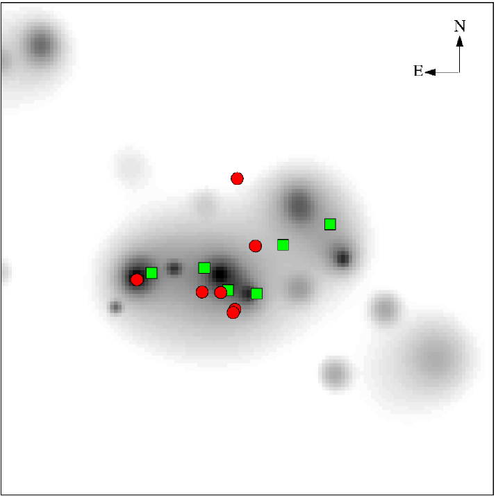
Figure 18: Projected galaxy density map (34$\times$34 ${\rm arcmin}^{2}$) of the red-sequence galaxies with $R_{\rm AB}<19$ (see Fig.6). The squares represent galaxies that are members of A3921 and classified as k+a and the circles as ”k+a?” (see text).

Figure 19: From left to right, velocity distribution (with a binning of 400 km/s) of k, k+a and emission line galaxies (according to the definition of Dressler et al. 1999, see text for details). In the central figure, the white component corresponds to secure k+a’s and the shaded part to k+a candidates. In the right panel, the shaded component of the histogram correspond to e(a)’s, the black component to e(b)’s, the white part to e(c) type objects.

In Fig. 18 we show the projected positions on the sky of secure k+a’s (squares) and k+a candidates (circles). From a simple visual inspection of this figure, most of k+a galaxies seem to be concentrated in projection around the central field of A3921-A. This is particularly clear in the case of k+a candidates, as only one of them is locate elsewhere, in the cluster outskirts. Confirmed k+a’s are less clustered around the central field of A3921-A. They are however concentrated in the highest density regions of the whole cluster and roughly aligned along an East/West direction. Applying a bi-dimensional Kolmogorov-Smirnov test, we cannot exclude that k+a’s spatial distribution is significantly different from that of k-type objects with a quite high significance level (87%). An intermediate and therefore not conclusive significance level (26%) is on the contrary obtained by comparing the projected positions of k+a candidates and passive galaxies.

The velocity distribution of the whole k+a sample is shown in the middle panel of Fig. 19. According to a visual inspection and usual statistical tests (i.e. 1D-KS, Rank-Sum, Hoel 1971, and F-tests, Press et al. 1992), it is not significantly different from the k-type’s velocity distribution (left panel). k+a candidates (shaded in Fig. 19) are characterized by a significantly higher velocity dispersion than passive and confirmed k+a galaxies (96% and 93% c.l. respectively according to an F-test), very close to the whole cluster value (1188 km/s $vs$ 1008 km/s, see Tables 8 and 2). Mean velocities of the different sub-samples are largely comparable within 1$\sigma$ errors.

7.3 Emission line galaxies

The emission-line population also shows interesting features, both in its fraction and colour distribution. We find 11 emission line galaxies, among which 2 starbursts (e(b)), 4 classical constant rate forming stars spirals (e(c)), and 5 e(a)-type objects, that have been suggested to be dust-starbursts (Poggianti et al., 1999). The global fraction of emission line galaxies (13%) is lower than that estimated at high redshift from MORPHS (26.5%), but comparable to that measured at intermediate redshifts ($0.18<z<0.55$) in the CNOC1 survey ($\sim$16%, Ellingson et al. 2001). Fig. 21 shows the ${\rm EW([OII])}$ as a function of V-R colour. The sample can be divided into two groups: the bluest ones with $V-R<0.3$, and typically large absolute values of ${\rm EW([OII])}$, ($<-10\AA)$, and the reddest ones with colours typical of the passive population $0.3<V-R<0.6$, and lower absolute values of ${\rm EW([OII])}$, $(\geq-10\AA)$, except for one object with an exceptionally strong [OII] line (${\rm EW([OII])}=-65\AA$), and a red colour index $V-R\sim 0.42$, which is identified with BG3. The presence of this red population of galaxies presenting emission lines is quite unusual, and reminiscent of what observed in the case of the merging cluster RX J0152.7-1357 at $z=0.837$ analysed by Demarco et al. 2004. This suggests that an on-going episode of star formation or bursting is occurring in an older population.

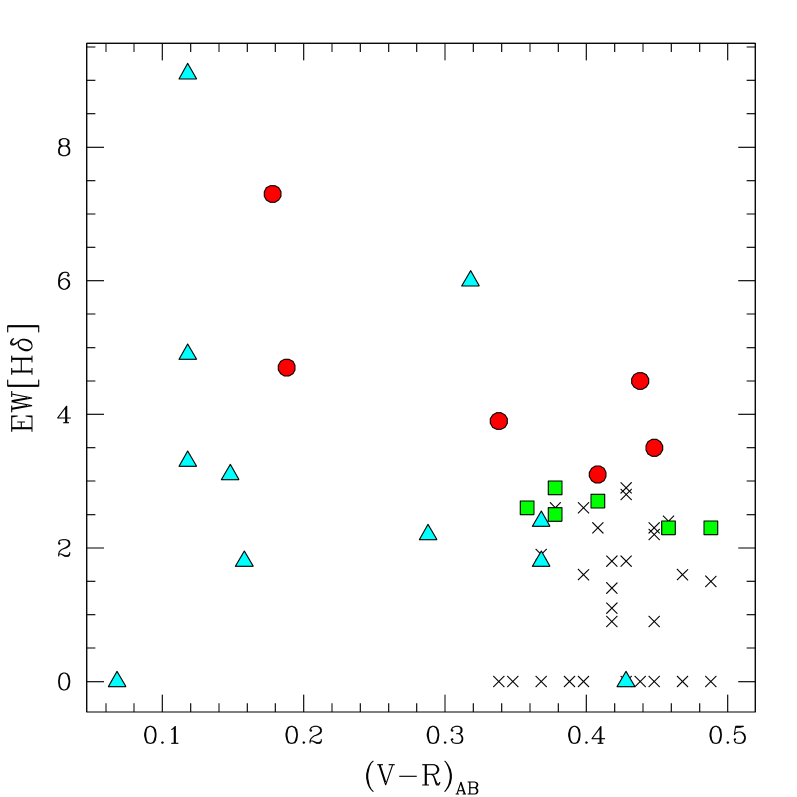
Figure 20: Colour-${\rm H}\delta$ diagram for galaxy members of A3921. Crosses indicate k type galaxies, squares k+a type galaxies, circles galaxies with H-K inversion and triangles emission lines galaxies.

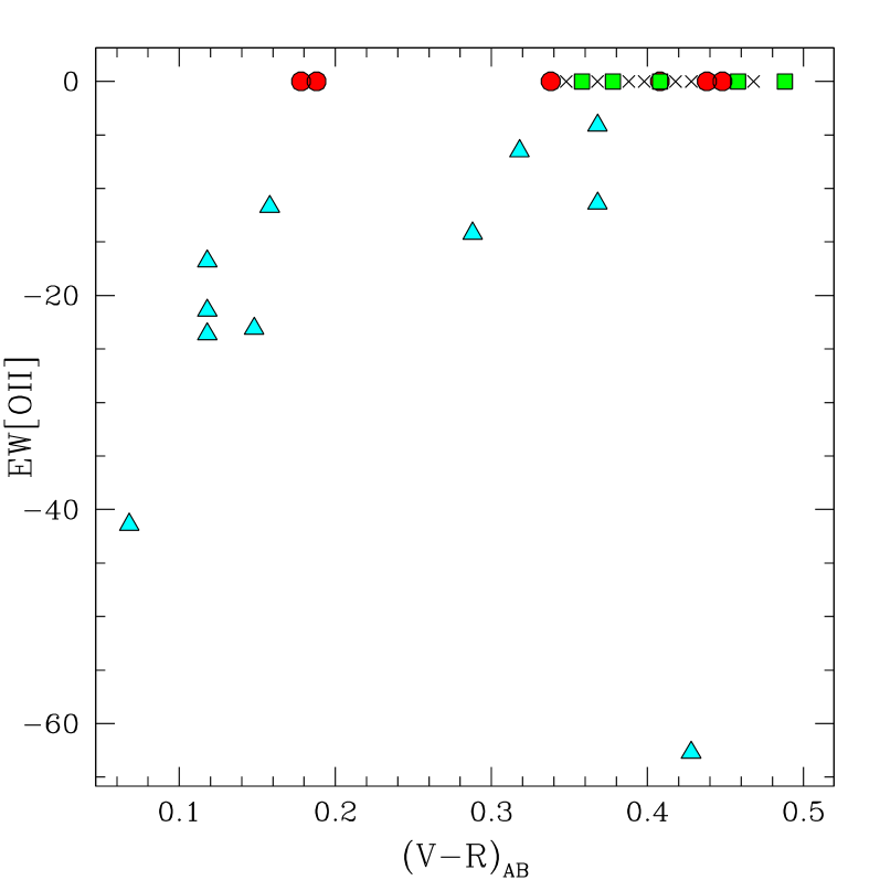
Figure 21: Colour-[OII] diagram for galaxy members of A3921. Crosses indicate k type galaxies, squares k+a type galaxies, circles galaxies with H-K inversion and triangles emission lines galaxies.

7.3.1 Spatial and velocity distributions

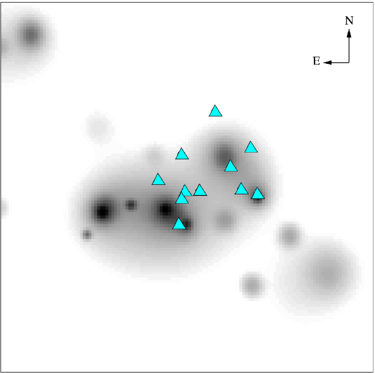
Figure 22: Projected galaxy density map (34$\times$34 ${\rm arcmin}^{2}$) of the red-sequence galaxies with $R_{\rm AB}<19$ (see Fig.6). The triangles show the location of emission line cluster member galaxies (see text).

Most (8/11) of star-forming galaxies seem to be spatially concentrated in the central region of the whole cluster, i.e. on the NW side of A3921-A, on the SE side and in the centre of A3921-B and between the two sub-clusters (see Fig. 22). A Rank-Sum test confirms this visual impression, as star-forming objects result more concentrated than k-type galaxies around a central position between the two subclusters with a very high c.l. (99.7%). Moreover, according to a bidimensional KS test, the spatial distributions of e-type and k-type galaxies are not drawn from the same parent population (2% significance level).

Fig. 19 shows that emission line galaxies have a much more dispersed velocity distribution with respect to passive objects. According to the F-test, velocity dispersion of emission line galaxies ($1607^{+314}_{-219}$ km/s) is significantly higher than the corresponding value for k-type objects ($770^{+119}_{-96}$ km/s), with a $\sim$100% confidence level.

Most of star-forming objects are therefore distributed between the two sub-clusters, and their velocity distribution is quite more dispersed than that of the relaxed k-type galaxies (whose velocity distribution does not differ significantly from a Gaussian), but with a comparable mean velocity. This suggests that, at least for a fraction of them, the star formation episode could be the result of an interaction with the ICM, connected with the merging process of the cluster.

7.4 SFR from [OII] equivalent widths

We will hereafter derive the SFR of the galaxies within A3921 from our measurements of the [OII] equivalent widths of our galaxy spectra. The uncertainties in the SFR estimated from [OII] are known to be larger than when derived through ${\rm H}\alpha$. This is due to the fact that, while flux estimates from ${\rm H}\alpha$ scale with the number of ionizing stars, estimates from [OII] are hampered by systematics due to large variations in excitation, implying substantial dispersions in the [OII]/${\rm H}\alpha$ and in the [OII]/${\rm H}\alpha$+[NII] correlations. In our case, however, [OII] is the only tracer of SFR available in our domain of wavelength, and will be used with caution. Using the equation derived by Kennicutt (1992):

$$SFR(M\mbox{${}_{\normalsize\odot}$}{\rm yr}^{-1})\sim 2.7\leavevmode\nobreak\ \times\leavevmode\nobreak\ 10^{-12}\leavevmode\nobreak\ \frac{L_{B}}{L_{B\sun}}{\rm EW(OII)}E({\rm H}\alpha)$$ (11)

the star-formation rate (SFR) is directly estimated from the integrated broad-band B luminosity, the [OII] equivalent width, assuming a reasonable value for the extinction correction $E({\rm H}\alpha)$. Converting our V-band magnitudes in B-band using $(B-V)_{AB}=0.65$ for the objects belonging to the red sequence and $(B-V)_{AB}=0.30$ for bluer objects, and taking a solar luminosity $M_{B}=5.48$, as well as the canonical value for extinction (1 mag for ${\rm H}\alpha$) used in Kennicutt 1992, we obtain an estimate of the SFR for our 11 galaxies with [OII] emission line. From the majority of spectra within A3921, the SFR ranges from 0.14 to $2.40M\mbox{${}_{\normalsize\odot}$}{\rm yr}^{-1}$, with however one object with very high SFR ($\sim 19.2M\mbox{${}_{\normalsize\odot}$}{\rm yr}^{-1}$) corresponding to the galaxy BG3 previously quoted. We estimate a median SFR of $\sim 0.58$ and a mean SFR of $\sim 0.72M\mbox{${}_{\normalsize\odot}$}{\rm yr}^{-1}$ (BG3 excluded). The cumulated SFR for the whole cluster reaches $\sim 11.5M\mbox{${}_{\normalsize\odot}$}{\rm yr}^{-1}$ (BG3 excluded). As expected, the values show that star formation in A3921 is suppressed as compared to field galaxies (Tresse and Maddox 1998). The highest optical SFR in our data apart from the BG3, ($2.40M\mbox{${}_{\normalsize\odot}$}{\rm yr}^{-1}$), is intermediate between the values obtained in A114 at $z=0.32$ by Couch et al. 2001 ($4M\mbox{${}_{\normalsize\odot}$}{\rm yr}^{-1}$), and that obtained by Duc et al. 2002 ($1.15M\mbox{${}_{\normalsize\odot}$}{\rm yr}^{-1}$) in Abell 1689 at $z=0.18$. However, the SFR in Couch et al. 2001 were measured with ${\rm H}\alpha$, and, as shown in Duc et al. 2002, measurements of the SFR with [OII] can be seriously underestimated due to dust extinction. Therefore our values can be considered as a lower limit of the SFR in A3921.

BG3 shows an exceptionally high star formation rate, suggesting a very active star-bursting object. The spectrum shows strong absorption lines typical of an old stellar population (Ca K and H, G band, $4000\AA$ break) as well as emission lines ([OII], ${\rm H}\gamma$ and ${\rm H}\beta$). Additional observations are planned to further investigate the nature of this object and to test if emission is due to star formation or to an active galactic nucleus (only the bluer part of the spectrum was obtained in these observations and the equivalent width of [OIII] is necessary to perform the test).

8 Discussion and conclusions

8.1 Dynamical state of the cluster

Using our new spectroscopic and VRI-bands photometric catalogues of the central $\sim\leavevmode\nobreak\ 1.8{\times}1.2\leavevmode\nobreak\ {\rm Mpc}^{2}$ region of A3921, we detect two main sub-clusters of galaxies: a South-East clump (A3921-A) that hosts the BCG (BG1), and, at $\sim$ 0.74 Mpc distance, a North-West system (A3921-B), hosting the second brightest cluster galaxy (BG2) and the third brightest object (BG3) in its outskirts. From the analysis of the projected density distribution, there are clear signs of merging events within this cluster. The density distribution of galaxies of A3921-A shows an elliptical shape, while A3921-B is characterized by a very morphologically disturbed distribution, with an extended low-density tail extending towards South. This morphology suggests that sub-cluster B is approaching cluster A from the North or exiting after colliding it from the South. The fact that the sub-cluster B is well defined would suggest that the merging has not yet occurred, but in case of a high impact parameter, or of a low mass ratio between the secondary and the main component, the density structure of the sub-clusters may survive. On the other hand, the presence of the Southern tail of subcluster B rather suggests a post-merger event. In this case, the tail would be made of faint galaxies lagging behind the brightest objects during their tangential crossing of subcluster A.

However, in spite of clear merging signatures on the density distribution, the kinematical and dynamical properties both of the whole cluster and of the two subclusters do not show strong signatures of merging. Moreover, the two sub-clusters show a very similar mean projected velocity. When applying a two-body dynamical model to the two components, several solutions could explain the observed dynamics of A3921 allowing both the pre-merging and the post-merging cases. A comparison with the X-ray properties of the cluster can allow us to discriminate between them. The analysis of XMM-Newton observations by Belsole et al. (2004) reveals that the X-ray emission of A3921-A can be modelled with a 2D$\beta$-model, leaving a distorted residual structure toward the NW, coincident with A3921-B (see Fig. 23). The main cluster detected in X-ray is centred on the BCG position (BG1), while the X-ray peak of the NW clump is offset from the brightest galaxy of A3921-B (BG2) (see Belsole et al. 2004). The temperature map of the cluster shows an extended hot region oriented parallel to the line joining the centres of the two sub-clusters. A comparison of this image with numerical simulations by Ricker & Sarazin (2001) suggests that we are observing the central phases of an off-axis merger between two unequal mass objects, where clump A is the most massive component (Belsole et al. 2004), consistent with optical results.

By combining the signatures of merging derived both from the optical iso-density map and from X-ray results, we can now reconsider the solutions of the two-body dynamical model (Table 6). In the pre-merger case, the high angle solutions of cases (a1) and (a2) would imply a very large real separation for the two sub-clusters ($\sim 6-7$ Mpc), which is very unlikely taking into account the clear signs of interaction between the two clumps observed both in optical and in X-ray. In the ”recent” post-merger case, we can also exclude the (c) solution, as we expect a higher value of the relative velocity ($\geq$1000 km/s) between the two clumps for obtaining a so evident hot bar in temperature map. Finally, the comparison of observed and simulated galaxy density and temperature maps (e.g. Schindler & Böhringer 1993, Ricker & Sarazin 2001) clearly exclude an older merger (e.g. $t_{0}$=1 Gyr), as we do not expect anymore to observe a clear bimodal morphology in optical and we should not detect such obvious structure in the temperature map. Therefore, only the solutions corresponding to the very central phases of merging ($t_{0}\approx\pm 0.3$ Gyr) can explain all our observational results, implying a collision axis nearly perpendicular to the line of sight. This is consistent with the absence of strong merging signatures in the observed projected velocity distribution of cluster members.

The superposition of the X-ray residuals onto the optical iso-density map (Fig. 23) shows that the bulk of X-ray emission in A3921-B is offset towards SW from the main concentration of galaxies. As numerical simulations show that the non-collisional component is much less affected by the collision than the gas distribution (e.g. Roettiger et al. 1993), this offset suggests that A3921-B is tangentially traversing A3921-A along a SW/NE direction, with its galaxies in advance with respect to the gaseous component. The off-axis collision geometry has probably prevented total assimilation of the B group into the main cluster A. This off-axis collision scenario is also consistent with the shape of the feature in the temperature map (Belsole et al. 2004).

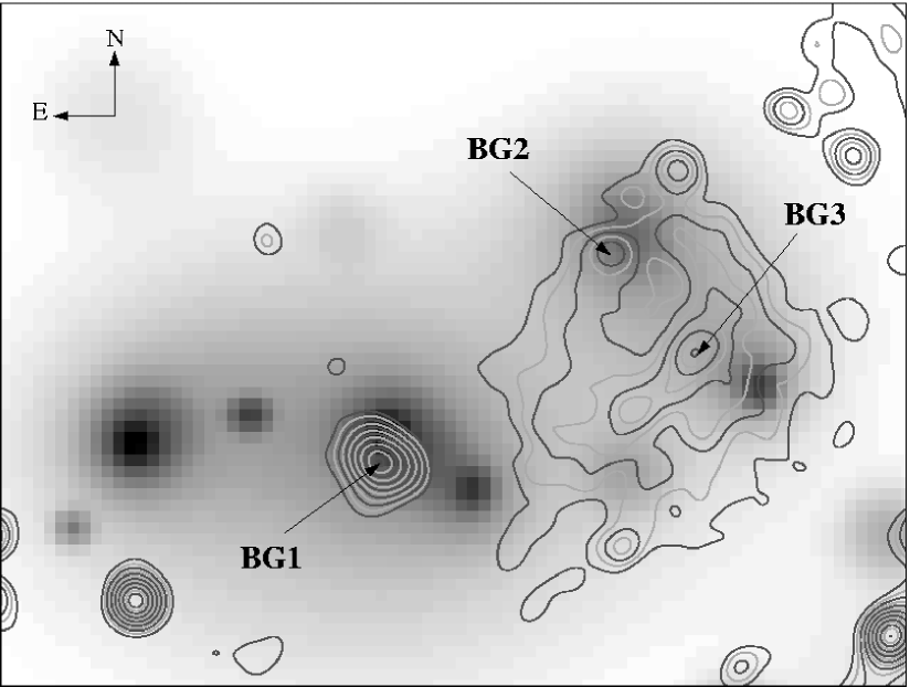
Figure 23: X-ray residuals after subtraction of a 2D-$\beta$ model (Belsole et al. 2004) overlaid on the red sequence galaxy density map of the central part of A3921 ($22\times 18{\rm arcmin}^{2}$).

8.2 Has the merging event affected star formation?

We detect very few k+a (1 secure and 3 candidates) at the bright absolute magnitude cut of MORPHS (Dressler et al. 1999). Most of our k+a and k+a? objects lie within $R_{AB}$ absolute magnitudes in the range [-19/-20]. This effect is very similar to the trend in luminosity detected by Poggianti et al. 2004 in Coma, but the typical luminosity of our k+a/k+a? objects is at least one magnitude brighter. However, we do not sample the faint end of the luminosity function as in the case of Coma, which may contain part of the undetected population. We therefore confirm the increase of the typical luminosity of the k+a population with redshift as detected in Poggianti et al. 2004, comparing Coma and MORPHS clusters. We also find a significant fraction of k+a in our low redshift cluster lying between the fractions obtained at low and high redshift. The mechanism responsible of this ”redshift” effect in A3921 is not immediate. This can be a ”redshift” consequence only due to some cosmic ”downsizing” effect, as it has been shown that the star formation activity at high $z$ was more efficient for more massive galaxies. In this case, this effect could be explained only by the infall of the galaxies into the cluster. On the other hand, A3921 shows very strong sub-clustering and signatures of merging, which can be suspected to be responsible, at least in some fraction, for the enhancement of the fraction of such objects. This will be detailed in the following.

The typical EW(H$\delta$) of the k+a/k+a? galaxies detected in A3921 is moderate and most of the objects have red colours, indistinguishable from red sequence objects. We fail to detect the population of blue k+a with strong Balmer lines as detected in Coma by Poggianti et al. 2004, which can only be reproduced by a starburst in a recent past. In contrast, our objects rather reflect the evolution of galaxies having undergone starburst or starforming activity, which has been suppressed by some physical process, and now lie in the second half of their lifetime (typically $<1.5$ Gyr), with redder colours, and fainter Balmer lines, before reaching a k-type spectrum. This population can be reproduced by simply halting star formation produced in continuous way, without evoking a strong star burst. The k+a? objects are probably galaxies having undergone a still older and fainter last episode of star formation, as they do not have Balmer lines strong enough to enter the k+a sample, but show clear signatures of past activity.

A fraction of emission line galaxies comparable to that found in intermediate redshift clusters has also been detected. The spatial and kinematical distributions of k+a and k+a? as well as emission line objects have been compared to the substructures evidenced both in the whole galaxy and gas distribution. While k+a/k+a? galaxies are mostly distributed among the main cluster A, the emission line galaxies mostly lie in the region of the sub-cluster B, and in the region in between A and B. A similar spatial distribution is followed by blue galaxies, which are more clustered in the central region of A3921-B than in the whole field and, in particular, than in the center of the more massive clump A (see Fig. 9). The comparison of the observed distributions of blue and emission line objects to the undergoing merging scenario presented previously ($\pm$ 0.3 Gyr) suggests that the interaction with the ICM during the passage of the sub-cluster B on the edge of the cluster A may have triggered star-bursting. This hypothesis is supported by the significant difference in the radial velocity dispersion of emission-line and passive galaxies, suggesting that emission-line objects are a dynamically younger population than the general cluster members. In contrast, the k+a/k+a? population shows a signature of an older star formation activity which can hardly be related to the on-going merger, but may be understood either as previously infalling galaxies, or relics from another older merging process, but now at rest within the main cluster, as shown from the velocity distribution.

Ongoing multi-wavelength (optical, X-ray and radio) follow-up will allow us to study in detail the environment and star formation properties of this cluster.

Appendix A Red sequence identification

The technique adopted to isolate the red sequence of the elliptical galaxies of A3921 and calculate its parameters (slope, intercept and width) is described in this Appendix.

The CMD of the central field of A3921 ($32{\times}32\leavevmode\nobreak\ {\rm arcmin}^{2}$) is shown in Fig. 7. Due to the high asymmetry of the galaxy distribution and the heavy contamination of field objects in our CMD, a simple linear regression plus an iterated 3$\sigma$ clip (Gladders et al. 1998) does not give satisfying results. We thus use the median absolute deviation (MAD) as scale indicator of the object distribution on our CMD, as it is extremely efficient ($\sim$90%) in the case of heavy-tailed distributions (Beers et al. 1990). In fact, we expect that, on the CMD, the deviations of the red sequence galaxies from the optimal linear fit follow a Gaussian distribution, while deviations of field objects do not and populate the tails of the distributions instead. We moreover apply an asymmetric clip (${n}_{i}{\cdot}{S}_{\rm MAD}$) on the two sides of the distribution (${n}_{1}-{n}_{2}=\sqrt[3]{skewness}/\sqrt{variance}$). We then follow a procedure similar to that described in Gladders et al., iterating our linear fitting and clipping until convergence on a final solution was obtained. The red sequence can be described by the linear equation $(R-I)_{\rm AB}=-0.0071I_{\rm AB}+0.5531$ with a width of $\sigma_{\rm RS}$=0.0837 (see Fig. 7).

Table 9: Spectroscopic data

#	R.A.	DEC.	$V_{\rm ab}$	$R_{\rm ab}$	$I_{\rm ab}$	$cz$	$\Delta$$cz$	Run	flag	EW([OII])	EW(${\rm H}_{\delta}$)	Type
	(J2000)	(J2000)				(km/s)	(km/s)			(Å)	(Å)
1	22:50:19.36	-64:25:50.7	17.95	17.52	17.06	28308.1	44.9	2001	1	0.0	1.8	k
2	22:50:16.39	-64:25:29.9	20.98	21.02	20.70	-2.0	-2.0	2001	1	-	-	-
3	22:50:12.08	-64:24:54.0	17.36	16.91	16.44	26858.1	38.1	2001	1	0.0	2.2	k
4	22:50:10.27	-64:24:20.8	18.73	18.04	17.47	-2.0	-2.0	2001	1	-	-	-
5	22:50:07.64	-64:24:28.5	18.86	18.68	18.39	27370.6	66.6	2001	1	0.0	7.3	k+a
6	22:50:01.78	-64:26:45.0	17.33	16.91	16.47	30339.4	36.2	2001	1	0.0	1.1	k
7	22:49:57.52	-64:24:44.3	17.71	17.25	16.78	27972.0	45.8	2001	1	0.0	2.4	k
8	22:49:54.76	-64:25:14.9	17.79	17.34	16.85	28023.1	34.7	2001	1	0.0	0.0	k
9	22:49:52.03	-64:26:02.6	19.48	19.14	18.49	28767.8	69.4	2001	1	0.0	3.9	k+a
10	22:49:47.61	-64:26:01.9	18.59	18.17	17.77	28129.0	45.3	2001	1	0.0	0.9	k
11	22:49:42.85	-64:25:05.9	19.62	19.55	19.75	-1.0	-1.0	2001	3	-	-	-
12	22:49:16.07	-64:22:48.4	19.19	19.00	18.69	27596.1	67.6	2001	1	0.0	4.7	k+a
13	22:49:13.03	-64:20:37.2	20.42	19.99	19.78	28183.9	74.7	2001	2	-	-	-
14	22:49:09.93	-64:20:06.8	20.37	20.10	19.81	26489.7	88.1	2001	2	-	-	-
15	22:49:06.62	-64:21:37.3	17.24	16.90	16.74	-2.0	-2.0	2001	1	-	-	-
16	22:49:04.91	-64:18:59.3	16.64	15.81	14.77	-2.0	-2.0	2001	1	-	-	-
17	22:48:58.98	-64:21:11.8	18.76	18.64	18.48	28141.7	98.3	2001	1	-23.6	3.3	e(a)
18	22:48:56.02	-64:20:13.8	20.65	20.35	20.46	27913.5	87.5	2001	2	-	-	-
19	22:48:53.06	-64:19:20.6	19.98	18.95	18.09	26110.5	89.2	2001	2	-	-	-
20	22:48:45.65	-64:21:24.5	18.03	17.58	17.26	28714.0	51.8	2001	1	0.0	3.5	k+a
21	22:48:42.86	-64:21:17.9	16.88	16.44	16.02	27804.7	31.7	2001	1	0.0	0.9	k
22	22:48:37.55	-64:20:14.2	20.26	19.87	19.64	25078.5	110.0	2001	2	-	-	-
23	22:48:35.94	-64:20:12.3	18.53	18.08	17.65	27781.7	80.6	2001	1	0.0	0.0	k
24	22:48:33.17	-64:20:50.4	19.29	18.65	18.19	25001.0	110.0	2001	2	-	-	-
25	22:49:45.36	-64:25:14.4	17.92	17.47	16.99	27572.9	52.2	2001	1	0.0	0.9	k
26	22:49:40.88	-64:26:34.5	19.45	19.06	18.61	27548.2	56.3	2001	1	0.0	0.0	k
27	22:49:38.06	-64:26:11.8	17.69	17.24	16.75	28607.6	50.8	2001	1	0.0	2.3	k
28	22:49:35.56	-64:26:07.2	16.86	16.49	16.12	28667.0	30.9	2001	1	0.0	1.9	k
29	22:49:28.71	-64:27:20.7	16.27	16.12	15.98	-2.0	-2.0	2001	1	-	-	-
30	22:49:27.39	-64:24:33.2	18.19	18.06	17.99	-2.0	-2.0	2001	1	-	-	-
31	22:49:24.24	-64:26:15.2	19.84	19.45	19.10	29559.6	84.0	2001	1	0.0	0.0	k
32	22:49:22.53	-64:23:42.0	18.67	17.98	17.24	24970.6	38.1	2001	2	-	-	-
33	22:49:18.94	-64:26:09.7	20.38	20.12	19.97	28585.7	132.6	2001	2	-	-	-
34	22:49:15.97	-64:25:30.8	19.59	18.72	17.33	20086.4	97.4	2001	2	-	-	-
35	22:49:12.36	-64:26:54.6	17.10	16.46	15.95	-2.0	-2.0	2001	1	-	-	-
36	22:49:07.62	-64:26:16.7	17.35	16.92	16.43	27997.9	32.7	2001	1	0.0	2.8	k
37	22:49:00.85	-64:26:05.5	19.05	18.68	18.28	28997.1	100.8	2001	1	0.0	0.0	k
38	22:50:13.53	-64:24:41.5	19.76	19.33	18.88	28876.6	98.4	2001	1	-	-	-
39	22:50:06.48	-64:24:41.9	16.37	15.92	15.48	28038.9	35.8	2001	1	0.0	0.0	k
40	22:50:04.72	-64:26:36.3	17.73	17.38	17.11	-2.0	-2.0	2001	1	-	-	-
41	22:49:58.18	-64:25:48.1	14.95	14.46	13.97	28166.4	64.2	2001	1	0.0	1.5	k
42	22:49:53.28	-64:25:03.5	18.01	17.54	17.06	28483.6	48.1	2001	1	0.0	1.6	k
43	22:49:48.42	-64:27:08.5	19.52	19.14	18.79	26969.9	76.4	2001	1	0.0	2.5	k+a?
44	22:49:45.45	-64:26:40.1	20.16	20.15	20.30	30435.3	173.2	2001	2	-	-	-
45	22:49:41.46	-64:26:24.1	19.68	19.31	18.96	25576.3	73.1	2001	1	-11.4	1.8	e(c)
46	22:49:38.74	-64:25:11.8	20.25	19.79	19.39	-1.0	-1.0	2001	3	-	-	-
47	22:49:36.32	-64:26:38.5	16.37	15.88	15.39	28061.1	46.8	2001	1	0.0	0.0	k
48	22:49:32.62	-64:26:13.9	19.70	19.26	18.78	27953.0	55.4	2001	1	0.0	4.5	k+a
49	22:49:12.28	-64:21:47.2	17.62	17.48	17.45	-2.0	-2.0	2001	1	-	-	-
50	22:49:09.53	-64:19:18.7	18.84	18.36	17.86	40663.7	107.4	2001	1	-	-	-

Table 10: Spectroscopic data

#	R.A.	DEC.	$V_{\rm ab}$	$R_{\rm ab}$	$I_{\rm ab}$	$cz$	$\Delta$$cz$	Run	flag	EW([OII])	EW(${\rm H}_{\delta}$)	Type
	(J2000)	(J2000)				(km/s)	(km/s)			(Å)	(Å)
51	22:49:07.26	-64:20:56.9	16.62	15.78	14.71	-2.0	-2.0	2001	1	-	-	-
52	22:49:04.78	-64:20:35.6	15.41	14.91	14.49	27888.4	38.5	2001	1	0.0	0.0	k
53	22:48:59.92	-64:20:50.4	16.48	16.05	15.56	27295.5	42.3	2001	1	0.0	0.0	k
54	22:48:54.08	-64:21:21.9	17.57	17.24	17.07	-2.0	-2.0	2001	1	-	-	-
55	22:48:50.71	-64:21:34.4	21.60	21.21	21.35	36279.8	113.3	2001	2	-	-	-
56	22:48:47.89	-64:20:34.5	19.21	18.79	18.39	27545.7	67.1	2001	1	0.0	0.0	k
57	22:48:39.66	-64:19:22.3	17.00	16.63	16.28	27151.0	52.5	2001	1	-4.1	2.4	e(c)
58	22:48:36.07	-64:22:38.4	17.61	17.20	16.73	27846.0	57.5	2001	1	0.0	2.7	k
59	22:48:35.42	-64:20:06.1	20.26	19.61	19.08	27878.7	94.4	2001	2	-	-	-
60	22:48:31.10	-64:19:51.9	20.67	19.77	19.23	27079.5	92.0	2001	2	-	-	-
61	22:48:29.29	-64:20:58.6	19.05	18.53	18.08	76835.2	90.7	2001	2	-	-	-
62	22:48:26.20	-64:20:50.1	17.60	17.51	17.53	-2.0	-2.0	2001	1	-	-	-
63	22:49:05.15	-64:25:03.5	16.61	16.38	16.19	-2.0	-2.0	2001	1	-	-	-
64	22:49:01.47	-64:25:04.0	18.06	17.63	17.12	28560.4	44.7	2001	1	0.0	0.0	k
65	22:49:00.10	-64:23:41.3	18.79	18.41	18.04	27953.0	58.7	2001	1	0.0	0.0	k
66	22:48:57.61	-64:23:59.4	19.54	18.62	17.91	32591.3	124.1	2001	2	-	-	-
67	22:48:53.47	-64:23:09.1	20.25	19.77	19.32	37746.2	58.5	2001	2	-	-	-
68	22:48:51.13	-64:23:10.1	20.50	20.34	19.86	-1.0	-1.0	2001	3	-	-	-
69	22:48:49.07	-64:23:12.0	16.21	15.78	15.33	29059.5	81.9	2001	1	-62.7	0.0	e(b)
70	22:48:44.80	-64:22:50.2	17.54	17.17	16.74	28186.1	38.7	2001	1	0.0	2.5	k
71	22:48:43.36	-64:23:53.1	18.60	18.30	17.99	28837.7	101.2	2001	1	0.0	2.1	k
72	22:48:38.08	-64:24:14.1	19.84	19.78	19.78	83738.0	112.5	2001	1	-	-	-
73	22:48:34.84	-64:23:39.9	17.95	17.66	17.26	28505.5	72.0	2001	1	-14.2	2.2	e(c)
74	22:48:29.27	-64:24:13.3	21.13	20.26	18.64	83383.1	120.4	2001	2	-	-	-
75	22:48:24.27	-64:23:42.9	19.46	18.65	17.49	-2.0	-2.0	2001	2	-	-	-
76	22:48:22.47	-64:21:26.7	16.68	16.49	16.41	-2.0	-2.0	2001	1	-	-	-
77	22:48:20.13	-64:21:58.2	19.39	18.97	18.65	-1.0	-1.0	2001	3	-	-	-
78	22:49:48.73	-64:21:47.2	15.96	15.71	15.58	-2.0	-2.0	2001	1	-	-	-
79	22:49:46.31	-64:25:12.0	19.15	18.72	18.30	27255.4	44.1	2001	1	0.0	0.0	k
80	22:49:44.51	-64:22:15.0	17.50	16.82	16.22	-2.0	-2.0	2001	1	-	-	-
81	22:49:41.10	-64:24:05.6	20.57	20.45	20.36	28957.4	46.4	2001	1	-21.4	9.1	e(a)
82	22:49:38.41	-64:23:23.8	19.00	18.88	18.75	29659.9	106.8	2001	1	-16.8	4.9	e(a)
83	22:49:35.31	-64:23:00.1	17.91	17.53	17.09	26168.7	34.1	2001	1	0.0	2.9	k+a?
84	22:49:36.63	-64:25:30.5	19.42	19.02	18.62	29173.6	45.9	2001	1	0.0	1.6	k
85	22:49:32.01	-64:21:44.1	19.77	19.41	19.01	25534.2	64.5	2001	2	-	-	-
86	22:49:28.71	-64:25:54.6	21.02	20.62	20.35	25415.1	92.7	2001	2	-	-	-
87	22:49:24.15	-64:23:01.5	21.63	21.66	21.49	15171.0	72.3	2001	2	-	-	-
88	22:49:19.41	-64:22:11.2	19.52	19.46	19.11	22355.2	90.2	2001	2	-	-	-
89	22:49:17.39	-64:22:56.0	20.67	20.49	20.19	25121.8	85.7	2001	2	-	-	-
90	22:49:15.13	-64:24:53.2	18.49	18.18	17.93	-2.0	-2.0	2001	1	-	-	-
91	22:49:07.81	-64:21:54.4	20.69	20.44	20.08	-1.0	-1.0	2001	3	-	-	-
92	22:49:04.37	-64:23:58.3	20.17	19.74	19.56	13836.7	98.9	2001	2	-	-	-
93	22:50:00.10	-64:18:43.8	19.88	19.44	19.18	-1.0	-1.0	2002	3	-	-	-
94	22:49:58.14	-64:20:05.8	18.92	18.50	18.11	30165.3	46.4	2002	1	0.0	0.0	k
95	22:49:54.60	-64:19:34.9	22.48	22.29	21.43	-1.0	-1.0	2002	3	-	-	-
96	22:49:50.74	-64:21:05.2	19.84	19.31	18.91	32423.2	140.8	2002	2	-	-	-
97	22:49:47.82	-64:19:04.4	15.20	15.12	15.17	-2.0	-2.0	2002	1	-	-	-
98	22:49:46.01	-64:18:14.1	17.60	17.22	16.90	27357.3	40.3	2002	1	0.0	2.9	k+a?
99	22:49:43.49	-64:20:07.5	20.00	19.60	19.23	77114.8	136.3	2002	1	-	-	-

Table 11: Spectroscopic data

#	R.A.	DEC.	$V_{\rm ab}$	$R_{\rm ab}$	$I_{\rm ab}$	$cz$	$\Delta$$cz$	Run	flag	EW([OII])	EW(${\rm H}_{\delta}$)	Type
	(J2000)	(J2000)				(km/s)	(km/s)			(Å)	(Å)
100	22:49:41.58	-64:19:59.0	18.38	18.31	18.46	25634.9	83.4	2002	1	-41.4	0.0	e(b)
101	22:49:39.50	-64:19:35.3	21.42	21.13	21.13	-1.0	-1.0	2002	3	-	-	-
102	22:49:36.68	-64:18:55.4	18.06	17.79	17.54	39792.0	82.8	2002	1	-	-	-
103	22:49:33.83	-64:20:14.1	20.76	20.11	19.74	136543.4	137.0	2002	2	-	-	-
104	22:49:33.39	-64:20:15.0	20.45	20.04	19.58	-1.0	-1.0	2002	3	-	-	-
105	22:49:30.17	-64:20:24.2	17.74	17.61	17.59	-2.0	-2.0	2002	1	-	-	-
106	22:49:28.53	-64:19:46.2	17.40	16.96	16.57	28093.8	36.1	2002	1	0.0	0.0	k
107	22:49:25.29	-64:19:26.3	17.61	17.38	17.29	-2.0	-2.0	2002	1	-	-	-
108	22:49:22.48	-64:19:03.6	18.45	17.96	17.56	40946.8	90.1	2002	1	-	-	-
109	22:49:18.63	-64:21:12.2	19.15	18.73	18.36	27983.8	48.1	2002	1	0.0	1.1	k
110	22:49:17.40	-64:19:55.1	21.95	20.84	20.02	-1.0	-1.0	2002	3	-	-	-
111	22:49:13.99	-64:19:04.8	21.77	21.11	20.83	-1.0	-1.0	2002	3	-	-	-
112	22:51:06.72	-64:25:12.9	-	-	-	33771.5	146.7	2002	1	-	-	-
113	22:51:05.11	-64:25:17.8	18.63	18.42	18.29	-2.0	-2.0	2002	1	-	-	-
114	22:51:03.17	-64:25:03.7	16.98	16.85	16.80	-2.0	-2.0	2002	1	-	-	-
115	22:51:01.34	-64:24:27.6	14.32	13.88	13.62	-2.0	-2.0	2002	1	-	-	-
116	22:50:58.45	-64:24:51.7	19.89	19.09	18.28	-2.0	-2.0	2002	1	-	-	-
117	22:50:56.78	-64:24:26.1	20.48	19.90	19.40	23657.6	79.5	2002	2	-	-	-
118	22:50:54.75	-64:26:00.5	18.31	18.18	18.13	-2.0	-2.0	2002	1	-	-	-
119	22:50:52.16	-64:25:13.1	19.15	18.79	18.43	29843.5	55.2	2002	1	0.0	2.6	k+a?
120	22:50:50.85	-64:25:20.8	17.86	17.46	17.04	28329.6	33.4	2002	1	0.0	2.6	k
121	22:50:48.31	-64:24:57.2	18.07	17.65	17.22	27611.2	37.8	2002	1	0.0	1.4	k
122	22:50:45.03	-64:24:25.0	16.95	16.48	16.03	27793.5	46.1	2002	1	0.0	0.0	k
123	22:50:44.28	-64:24:19.4	16.05	15.88	15.80	-2.0	-2.0	2002	1	-	-	-
124	22:50:41.83	-64:24:46.2	19.27	18.86	18.48	27303.1	76.7	2002	1	0.0	3.1	k+a
125	22:50:39.80	-64:23:31.1	19.24	19.01	18.79	-2.0	-2.0	2002	1	-	-	-
126	22:50:36.92	-64:24:08.4	17.26	17.18	17.17	-2.0	-2.0	2002	1	-	-	-
127	22:50:33.55	-64:22:39.2	18.09	17.68	17.24	33096.0	77.1	2002	2	-	-	-
128	22:50:30.31	-64:25:46.0	17.60	17.45	17.40	-2.0	-2.0	2002	1	-	-	-
129	22:50:26.53	-64:24:32.0	18.09	17.69	17.26	26487.6	52.2	2002	1	0.0	2.3	k
130	22:50:24.77	-64:24:39.7	18.35	17.97	17.59	26285.7	66.9	2002	1	0.0	2.6	k
131	22:50:23.61	-64:23:06.5	18.73	18.24	17.77	28336.1	85.2	2002	1	-	-	-
132	22:50:21.57	-64:26:43.2	19.75	19.00	18.08	-2.0	-2.0	2002	1	-	-	-
133	22:50:19.49	-64:26:28.1	18.37	17.94	17.50	28223.9	40.3	2002	1	0.0	0.0	k
134	22:50:15.19	-64:27:53.0	18.68	18.28	17.89	26234.3	57.7	2002	1	0.0	0.0	k
135	22:50:14.46	-64:26:06.5	16.43	16.23	16.10	-2.0	-2.0	2002	1	-	-	-
136	22:50:07.83	-64:26:02.1	19.69	19.23	18.76	27787.5	64.8	2002	1	0.0	2.3	k+a?
137	22:50:05.87	-64:27:20.2	15.21	15.09	15.05	-2.0	-2.0	2002	1	-	-	-
138	22:50:02.53	-64:27:54.7	21.08	20.77	20.62	32474.3	47.4	2002	2	-	-	-
139	22:49:59.65	-64:26:40.6	14.76	14.64	14.60	-2.0	-2.0	2002	1	-	-	-
140	22:49:58.13	-64:26:05.4	18.67	18.18	17.61	27843.1	79.3	2002	1	0.0	2.3	k+a?
141	22:49:55.09	-64:24:41.8	19.07	18.64	18.22	27381.9	58.1	2002	1	0.0	0.0	k
142	22:49:51.65	-64:26:00.0	19.42	19.04	18.39	27507.3	50.8	2002	1	0.0	2.6	k
143	22:49:48.34	-64:27:01.1	20.63	20.22	19.99	29371.5	88.4	2002	1	0.0	2.7	k+a?
144	22:49:46.78	-64:25:38.4	19.67	19.24	18.78	28997.3	86.8	2002	1	0.0	2.9	k
145	22:49:43.23	-64:25:16.6	19.82	19.71	19.78	50679.8	109.3	2002	2	-	-	-
146	22:49:41.37	-64:26:11.9	22.15	21.27	19.79	-1.0	-1.0	2002	3	-	-	-
147	22:49:37.90	-64:27:09.2	18.51	18.11	17.67	28941.8	54.6	2002	1	0.0	0.0	k
148	22:49:34.88	-64:25:53.2	21.64	20.70	19.19	-1.0	-1.0	2002	3	-	-	-
149	22:49:24.16	-64:20:14.7	-0.01	22.36	21.30	24260.9	112.1	2002	2	-	-	-
150	22:49:19.12	-64:22:10.0	-0.01	21.14	19.83	76517.1	97.8	2002	1	-	-	-

Table 12: Spectroscopic data

#	R.A.	DEC.	$V_{\rm ab}$	$R_{\rm ab}$	$I_{\rm ab}$	$cz$	$\Delta$$cz$	Run	flag	EW([OII])	EW(${\rm H}_{\delta}$)	Type
	(J2000)	(J2000)				(km/s)	(km/s)			(Å)	(Å)
151	22:49:18.82	-64:22:06.2	20.52	20.23	19.80	76278.4	68.1	2002	1	-	-	-
152	22:49:14.86	-64:21:59.7	19.34	18.99	18.75	45803.5	56.2	2002	1	-	-	-
153	22:49:12.26	-64:19:41.7	16.44	15.57	14.31	-2.0	-2.0	2002	1	-	-	-
154	22:49:10.31	-64:18:30.4	17.63	17.15	16.67	28212.5	70.2	2002	1	0.0	0.0	k
155	22:49:06.83	-64:19:33.3	18.50	18.08	17.67	28019.9	65.0	2002	1	0.0	0.0	k
156	22:49:04.07	-64:19:59.1	18.46	17.99	17.52	28299.3	37.5	2002	1	0.0	0.0	k
157	22:49:02.03	-64:20:24.9	16.85	16.14	15.61	-2.0	-2.0	2002	1	-	-	-
158	22:48:59.87	-64:21:24.9	22.26	21.94	0.49	-1.0	-1.0	2002	3	-	-	-
159	22:48:56.84	-64:22:42.1	21.22	20.82	20.50	26253.3	82.2	2002	1	-	-	-
160	22:48:54.48	-64:22:38.3	20.82	20.52	20.28	20990.9	64.0	2002	2	-	-	-
161	22:48:52.09	-64:21:07.0	22.08	21.39	20.51	11581.2	88.8	2002	2	-	-	-
162	22:48:49.32	-64:21:49.9	16.94	16.72	16.63	-2.0	-2.0	2002	1	-	-	-
163	22:48:50.72	-64:19:31.8	12.81	12.81	12.52	-2.0	-2.0	2002	1	-	-	-
164	22:48:47.80	-64:19:57.6	21.88	20.93	19.55	25499.4	106.2	2002	2	-	-	-
165	22:48:44.29	-64:19:56.7	19.23	18.76	18.31	47378.9	80.4	2002	1	-	-	-
166	22:48:40.06	-64:20:55.8	18.15	18.11	18.14	-1.0	-1.0	2002	3	-	-	-
167	22:48:39.63	-64:21:25.3	19.68	18.97	18.47	35278.8	49.3	2002	1	-	-	-
168	22:50:04.02	-64:22:12.1	19.51	19.04	18.72	26820.6	112.9	2002	2	-	-	-
169	22:50:01.83	-64:22:21.8	18.26	17.94	17.66	25417.1	65.1	2002	1	-6.5	6.0	e(a)
170	22:50:00.12	-64:23:04.7	16.99	16.78	16.67	-2.0	-2.0	2002	1	-	-	-
171	22:49:58.23	-64:23:23.8	20.60	19.74	18.72	39858.5	84.7	2002	2	-	-	-
172	22:49:55.83	-64:22:37.8	17.44	17.39	17.41	-2.0	-2.0	2002	1	-	-	-
173	22:49:54.00	-64:23:43.1	19.22	18.91	18.50	27002.7	57.0	2002	1	0.0	1.6	k
174	22:49:47.53	-64:21:24.4	19.58	19.43	19.34	31631.0	86.0	2002	2	-	-	-
175	22:49:44.99	-64:23:00.7	19.70	19.24	18.88	28404.3	78.6	2002	1	0.0	0.0	k
176	22:49:42.54	-64:23:36.0	23.03	21.94	20.06	-1.0	-1.0	2002	3	-	-	-
177	22:49:38.28	-64:23:37.1	20.12	19.95	19.86	-2.0	-2.0	2002	2	-	-	-
178	22:49:34.50	-64:24:15.4	19.68	19.27	18.85	28796.8	96.5	2002	1	0.0	1.6	k
179	22:49:29.94	-64:21:33.7	19.55	19.38	19.41	-1.0	-1.0	2002	3	-	-	-
180	22:49:30.53	-64:24:14.6	17.15	16.98	16.85	38735.5	86.2	2002	2	-	-	-
181	22:49:26.08	-64:23:21.4	19.15	18.99	18.78	28360.1	98.0	2002	1	-11.7	1.8	e(c)
182	22:49:24.12	-64:25:18.6	17.84	17.14	16.48	-2.0	-2.0	2002	1	-	-	-
183	22:49:22.39	-64:23:05.4	19.08	18.95	18.87	-2.0	-2.0	2002	1	-	-	-
184	22:49:18.45	-64:25:04.0	20.62	20.53	20.54	25393.9	108.5	2002	2	-	-	-
185	22:49:14.39	-64:24:43.7	19.84	19.70	19.62	29093.6	102.2	2002	2	-	-	-
186	22:49:11.77	-64:25:18.0	17.84	17.45	16.97	29982.7	42.6	2002	1	0.0	0.0	k
187	22:49:07.77	-64:24:28.6	20.25	20.07	19.82	-1.0	-1.0	2002	3	-	-	-
188	22:49:01.75	-64:24:39.3	20.72	20.10	19.55	-1.0	-1.0	2002	3	-	-	-
189	22:48:58.93	-64:23:54.6	18.84	18.63	18.13	29194.9	92.6	2002	2	-	-	-
190	22:48:52.22	-64:25:16.6	18.77	18.19	17.72	-2.0	-2.0	2002	1	-	-	-
191	22:48:50.13	-64:24:21.5	19.62	19.31	18.84	-1.0	-1.0	2002	3	-	-	-
192	22:48:47.44	-64:22:33.0	20.61	20.12	19.77	-1.0	-1.0	2002	3	-	-	-
193	22:48:45.58	-64:24:17.8	20.18	19.88	19.55	-1.0	-1.0	2002	3	-	-	-
194	22:48:43.82	-64:24:35.9	18.29	17.83	17.36	34446.7	84.3	2002	2	-	-	-
195	22:48:41.31	-64:24:06.4	21.10	20.83	20.61	-1.0	-1.0	2002	3	-	-	-
196	22:48:39.21	-64:22:20.8	13.23	13.30	13.09	-2.0	-2.0	2002	1	-	-	-
197	22:48:37.35	-64:24:06.5	18.51	18.14	17.76	26677.0	70.2	2002	1	0.0	0.0	k
198	22:48:34.45	-64:24:58.4	19.94	19.60	19.31	27698.2	97.0	2002	1	0.0	0.0	k
199	22:48:33.81	-64:23:45.6	18.86	18.48	18.08	28454.0	98.3	2002	1	0.0	0.0	k

Table 13: Spectroscopic data

#	R.A.	DEC.	$V_{\rm ab}$	$R_{\rm ab}$	$I_{\rm ab}$	$cz$	$\Delta$$cz$	Run	flag	EW([OII])	EW(${\rm H}_{\delta}$)	Type
	(J2000)	(J2000)				(km/s)	(km/s)			(Å)	(Å)
200	22:48:30.44	-64:24:04.7	22.20	21.20	19.62	-1.0	-1.0	2002	3	-	-	-
201	22:49:35.77	-64:29:49.2	20.14	19.50	18.94	87248.7	141.3	2002	2	-	-	-
202	22:49:34.06	-64:28:14.1	21.94	21.18	19.76	-1.0	-1.0	2002	3	-	-	-
203	22:49:31.64	-64:28:27.5	19.63	19.14	18.66	-1.0	-1.0	2002	3	-	-	-
204	22:49:29.66	-64:28:31.9	18.72	18.58	18.37	40483.6	78.4	2002	2	-	-	-
205	22:49:27.93	-64:26:24.8	19.31	18.55	17.32	12633.3	60.3	2002	2	-	-	-
206	22:49:24.90	-64:27:36.8	19.89	19.50	19.13	27849.3	95.7	2002	2	-	-	-
207	22:49:20.99	-64:28:57.9	18.18	17.74	17.26	27776.3	37.0	2002	1	0.0	0.0	k
208	22:49:19.29	-64:27:13.7	19.36	19.08	18.65	-1.0	-1.0	2002	3	-	-	-
209	22:49:17.23	-64:28:56.6	17.09	16.35	15.58	-2.0	-2.0	2002	1	-	-	-
210	22:49:14.03	-64:29:42.8	18.29	17.88	17.42	26797.2	44.8	2002	1	0.0	2.3	k
211	22:49:12.50	-64:26:43.4	18.16	17.72	17.31	27003.7	68.7	2002	1	0.0	0.0	k
212	22:49:09.29	-64:30:56.8	16.07	15.73	15.41	-2.0	-2.0	2002	1	-	-	-
213	22:49:07.63	-64:28:09.7	17.54	16.93	16.37	-2.0	-2.0	2002	1	-	-	-
214	22:49:04.75	-64:26:17.7	20.76	19.99	19.25	-1.0	-1.0	2002	2	-	-	-
215	22:49:02.68	-64:27:43.5	19.59	19.64	19.90	19608.5	77.4	2002	2	-	-	-
216	22:49:00.93	-64:28:11.1	17.89	17.54	17.10	26430.9	59.0	2002	1	0.0	0.0	k
217	22:48:58.19	-64:27:50.7	19.28	18.88	18.19	18467.1	57.0	2002	2	-	-	-
218	22:48:56.40	-64:29:20.7	16.36	16.23	16.14	-2.0	-2.0	2002	1	-	-	-
219	22:48:54.53	-64:28:35.8	20.55	20.28	19.32	-1.0	-1.0	2002	3	-	-	-
220	22:48:52.71	-64:29:09.1	19.21	18.80	18.52	29057.8	62.7	2002	2	-	-	-
221	22:48:51.24	-64:29:08.7	17.49	17.07	16.72	28386.4	34.3	2002	1	0.0	1.8	k
222	22:49:21.73	-64:16:08.2	16.48	16.30	16.22	-2.0	-2.0	2003	1	-	-	-
223	22:49:19.93	-64:13:54.9	18.53	18.22	17.97	28380.3	86.0	2003	2	-	-	-
224	22:49:17.16	-64:15:40.8	14.80	14.64	14.62	-2.0	-2.0	2003	1	-	-	-
225	22:49:14.54	-64:16:08.0	19.83	19.78	19.81	-2.0	-2.0	2003	1	-	-	-
226	22:49:11.96	-64:16:03.9	19.27	19.12	19.00	29965.4	129.5	2003	1	-23.1	3.1	e(a)
227	22:49:08.89	-64:15:38.1	18.40	18.10	17.79	40723.0	146.7	2003	1	-	-	-
228	22:49:07.60	-64:15:27.3	17.87	17.35	16.88	49673.1	62.7	2003	1	-	-	-
229	22:49:04.62	-64:14:31.9	18.73	17.86	16.46	-2.0	-2.0	2003	2	-	-	-
230	22:49:02.23	-64:16:39.5	20.27	19.97	19.67	40621.9	77.9	2003	1	-	-	-
231	22:49:00.69	-64:14:38.1	19.62	18.90	18.35	25789.2	81.1	2003	2	-	-	-
232	22:48:58.22	-64:14:44.3	17.30	17.13	17.07	-2.0	-2.0	2003	2	-	-	-
233	22:48:55.85	-64:13:34.2	14.28	14.13	14.13	-2.0	-2.0	2003	2	-	-	-
234	22:48:55.80	-64:15:21.8	14.11	13.78	13.57	-2.0	-2.0	2003	2	-	-	-
235	22:48:50.54	-64:14:03.7	17.65	17.40	17.21	26343.0	54.0	2003	2	-	-	-
236	22:48:48.00	-64:15:46.3	21.90	21.13	20.73	25494.6	80.5	2003	2	-	-	-
237	22:48:45.29	-64:15:46.0	17.92	17.53	17.16	28166.1	41.7	2003	1	0.0	1.6	k
238	22:48:44.06	-64:13:43.2	19.35	19.25	19.15	31409.4	58.5	2003	2	-	-	-
239	22:48:39.53	-64:16:22.1	20.96	20.30	19.75	33496.9	127.2	2003	2	-	-	-

References

- (1) Abraham, R.G., Snecker-Hane, T.A., Hutchings, J.B., Carlberg, R.G., Yee, H.K.C., Ellingson, E., Morris, S., Oke, J.B., & Rigler, M., 1996, ApJ, 471, 694
- (2) Arnaud, M., Maurogordato, S., Slezak, E., & Rho, J., 2000, A&A, 355, 461
- (3) Arnaud, M., Rothenflug, R., Böhringer, H., Neumann, D., & Yamashita, K., 1996, uxsa.coll, 163
- (4) Arnouts, S., Vandame, B., Benoist, C. et al. 2001, A&A, 379, 740
- (5) Ashman, K.M., Bird, C.M., & Zepf, S., 1994, AJ, 108, 2348
- (6) Balogh, M.L., Morris, S.L., Yee, H.K.C., Carlberg, R.G., & Ellingson, E., 1999, ApJ, 527, 54
- (7) Balogh, M.L., Shade, D., Morris, S.L., Yee, H.K.C., Carlberg, R.G., & Ellingson, E., 1998, ApJL, 504, 75
- (8) Balogh, M.L., Morris, S.L., Yee, H.K.C., Carlberg, R.G., & Ellingson, E., 1997, ApJL, 488, 75
- (9) Baldi, A., Bardelli, S., & Zucca, E., 2001, MNRAS, 324, 509
- (10) Barrena, R., Biviano, A., Ramella, M., Falco, E.E., & Seitz, S., 2002, A&A, 386, 861B
- (11) Bekki, K., 1999, ApJL, 510, 15
- (12) Belsole, E., Sauvageot, J.-L., Pratt, G.W., & Bourdin, H., 2004, submitted to A&A
- (13) Beers, T. C., Gebhardt, K., Huchra, J.P., Forman, W., Jones, C., & Bothun, G.D., 1992, ApJ, 400, 410
- (14) Beers, T. C., Flynn, K., & Gebhardt, K., 1990, AJ, 100, 32
- (15) Bertin, E. & Arnouts, S. 1996, A&AS, 117, 393
- (16) Bijaoui A., & Rué F. A Vision Model adapted to the astronomical images Signal Processing v.46 n.3 pp. 345-362 1995
- (17) Bird, C. M., Davis, S. D., & Beers, T. C., 1995, AJ, 109, 920
- (18) Bird, C. M., 1994, AJ, 107, 1637
- (19) Bird, C. M., & Beers, T. C., 1993, AJ, 105, 1596
- (20) Biviano, A., Katgert, P., Mazure, A., Moles, M., den Hartog, R., Perea, J., & Focardi, P., 1997, A&A, 321, 84
- (21) Caldwell, N., Rose, J.A., Sharples, R.M., Ellis, R.S. & Bower, R.G., 1993, AJ, 106, 473
- (22) Carlberg, R.G., Yee, H.K.C., Ellingson, E., Abraham, R., Gravel, P., Morris, S., & Pritchet, C.J., 1996, ApJ, 462, 32
- (23) Couch, W.J. & Sharples, R.M., 1987, MNRAS, 229, 423
- (24) Couch, W.J., Balogh, M.L., Bower, R.G., Smail, I. Glazebrook, K. & Taylor, M., 2001, ApJ, 549, 820
- (25) Davis, D.S., Bird, C.M., Mushotzky, R.F., & Odewahn, S.C., 1995, ApJ, 440, 48
- (26) Demarco, R., 2004, PhD thesis, University of Paris 7, France
- (27) den Hartog, R., & Katgert, P, 1996, MNRAS, 279, 349
- (28) Donnelly, R.H., Forman, W., Jones, C., Quintana, H., Ramirez, A., Churazov, E., & Gilfanov, M., 2001, ApJ, 562, 254
- (29) Dressler, A., & Gunn, J.E., 1983, ApJ, 270, 7
- (30) Dressler A., Smail, I., Poggianti, B.M., Butcher, H., Couch, W.J., Ellis, R.S., & Oemler, A., 1999, ApJ, 122, 51
- (31) Dressler A., & Shectman, S., 1988, AJ, 95, 985
- (32) Dressler A., 1987, in Nearly Normal Galaxies: From the Planck Time to the Present, ed S. Faber (New York: Springer), 276
- (33) Duc, P.A., Poggianti, B.M., Fadda, D., Elbaz, D., Flores, H., Chanila, P., Franceschini, A., Moorwood, A., & Cesarsky, C., 2002, A&A, 382, 60
- (34) Durret, F., Forman, W., Gerbal, D., Jones, C., & Vikhlinin, A., 1998, A&A, 335, 41
- (35) Eke V.R., Cole S., & Frenk C.S., 1996, MNRAS 282, 263
- (36) Ellingson, E., Lin, H., Yee, H.K.C., & Carlberg, R.G., 2001, ApJ, 547, 609
- (37) Evrard, A.E., 1991, MNRAS, 248, 8
- (38) Fadda, D., Slezak, E. & Bijaoui, A., 1998, A&AS, 127, 335
- (39) Fadda, D., Girardi, M., Giuricin, G., Mardirossian, F., & Mezzetti, M., 1996, ApJ, 473, 670
- (40) Ferrari, C., Maurogordato, S., Cappi, A., & Benoist, C., 2003, A&A, 399, 813
- (41) Flores, R.A., Quintana, H., & Way, M.J., 2000, ApJ, 532, 206
- (42) Franx, M., 1993, PASP, 105, 1058
- (43) Fujita, Y., Takizawa, M., Nagashima, M., & Enoki, M., 1999, PASJ, 51, L1
- (44) Gavazzi, G., Cortese, L., Boselli, A., Iglesias-Paramo, J., Vílchez, J.M., & Carrasco, L., 2003, ApJ, 597, 210
- (45) Girardi, M., Giuricin, G., Mardirossian, F., Mezzetti, M., & Boschin, W., 1998, ApJ, 505, 74
- (46) Gladders, M. D., Lopez-Cruz, O., Yee, H. K. C., & Kodama, T., 1998, ApJ, 501, 571
- (47) Gregory, S.A., & Thompson, L.A., 1984, ApJ, 286, 422
- (48) Hartigan, J. A., & Hartigan, P. M., 1985, The Annals of Statistics, Vol.13, No. 1, 70-84
- (49) Hoel, P.G., 1971, Introduction to Mathematical Statistics, New York: J. Wiley & Sons
- (50) Jones, C., & Forman, W., 1992, Clusters and Superclusters of Galaxies, edited by A.C. Fabian, (Kluwer, Dordrecht), pp. 49-70
- (51) Katgert, P., Biviano, A., & Mazure, A., 2004, ApJ, 600, 657
- (52) Katgert, P., Mazure, A., den Hartog, R., Adami, C., Biviano, A., & Perea, J., 1998, A&AS, 129, 399
- (53) Katgert, P., Mazure, A., Perea, J., den Hartog, R., Moles, M., et al. 1996, A&A, 310, 8
- (54) Kauffmann, G., 1995, MNRAS, 274, 153
- (55) Kauffmann, G., 1995, MNRAS, 274, 161
- (56) Kennicutt, R.C. Jr, 1992, ApJ, 388, 310
- (57) Landolt, A.U. 1992, AJ, 104, 340
- (58) Lemonon, L., Pierre, M., Hunstead, R., Reid, A., Mellier, Y., & Böhringer, H., 1997, A&A, 326, 34
- (59) Limber, N.D., & Mathews, W.G., 1960, ApJ, 132, 286
- (60) Markevitch, M., Ponman, T.J., Nulsen, P.E.J., Bautz, M.W., Burke, D.J., David, L.P., Davis, D., Donnelly, R.H., Forman, W.R., Jones, C., Kaastra, J., Kellogg, E., Kim, D.W., Kolodziejczak, J., Mazzotta, P., Pagliaro, A., Patel, S., Van Speybroeck, L., Vikhlinin, A., Vrtilek, J., Wise, M., & Zhao, P., 2000, ApJ, 541, 542
- (61) Mazure, A., Katgert, P., den Hartog, R., Biviano, A., Dubath, P., Escalera, E., Focardi, P., Gerbal, D., Giuricin, G., Jones, B., Le Fèvre, O., Moles, M., Perea, J., & Rhee, G., 1996, A&A, 310, 31
- (62) McLachlan, G. J., Basford, K. E., 1988, Mixture Models (Marcel Dekker, New York)
- (63) Moss, C., & Whittle, M., 2000, MNRAS, 317, 667
- (64) Muriel, H., Quintana, H., Infante, L., Lambas, D.G., & Way, M.J., 2002, AJ, 124, 1934
- (65) Navarro, J.F., Frenk, C.S., & White, S.D.M., 1997, ApJ, 490, 493
- (66) Newberry, M.V., Boronson, T.A., & Kirshner, R.P., 1990, ApJ, 350, 585
- (67) Nikogossyan, E., Durret, F., Gerbal, D., & Magnard, F., 1999, A&A, 349, 97
- (68) Poggianti, B.M., Bridges, T.J., Komiyama, Y., Yagi, M., Carter, D., Mobasher, B., Okamura, S., & Kashikawa, N., 2004, ApJ, 601, 197
- (69) Poggianti, B.M., Smail, I., Dressler, A., Couch, W.J., Barger, A.J., Butcher, H., Ellis, R.S., & Oemler, A., 1999, ApJ, 518, 576
- (70) Postman, M., Lubin, L.M., & Oke, J.B., 1998, AJ, 116, 560
- (71) Press, W.H, Teukolsky, S.A., Vetterling, W.T., & Flannery, B.P., 1992, Numerical Recipes, Cambridge: Cambridge University Press
- (72) Quintana, H., Ramírez, A., & Way, M.J., 1996, AJ, 112, 36
- (73) Ricker, P.M., & Sarazin, C.L., 2001, ApJ, 561, 621R
- (74) Roettiger, K., Stone, J.M. & Mushotzky. R.F., 1998, ApJ, 493, 62
- (75) Roettiger, K., Burns, J., & Loken, C., 1993, ApJ, 407, L53
- (76) Rose, J.A., 1985, AJ, 90, 1927
- (77) Rué F., & Bijaoui A.: A Multiscale Vision Model to Analyze field astronomical images Experimental Astronomy 7 pp. 129-160 1997
- (78) Sarazin, C.L., 2003, astro-ph/0301178
- (79) Sauvageot, J.L., Belsole, E., Arnaud, M., & Ponman, T.J., 2001, in Clusters of galaxies and the high redshift universe observed in X-ray, Recent results of XMM-Newton and Chandra, XXXVIth Rencontres de Moriond, XXIst Moriond Astrophysics Meeting, Edited by D. Neumann & J.T.T. Van
- (80) Schindler, S., & Böhringer, H., 1993, A&A, 269, 83
- (81) Schindler, S., & Müller, E., 1993, A&A, 272, 137
- (82) Schlegel, D., Finkbeiner, D., & Davis, M. 1998, ApJ, 500, 525
- (83) Tomita, A., Nakamura, F.E., Takata, T., Nakanishi, K., Takeuchi, T., Ohta, K., & Yamada, T., 1996, AJ, 111, 42
- (84) Tonry, J., & Davis, M., 1981, ApJ, 246, 666
- (85) Tran, K.-V.H., Franx, M., Illingworth, G., Kelson, D.D., & van Dokkum, P., 2003, ApJ, 599, 865
- (86) Tresse, L., & Maddox, S.J., 1998, ApJ, 495, 691
- (87) Wang, Q.D., Ulmer, M.P., & Lavery, R.J., 1997, MNRAS, 288, 702
- (88) West, M. J., Jones, C., & Forman, W., 1995, ApJL, 451, 5
- (89) West, M. J., & Bothun, G. D., 1990, ApJ, 350, 36
- (90) Yahil, A., & Vidal, N., 1977, ApJ, 214, 347