The 2dF-SDSS LRG and QSO Survey: The LRG 2-Point Correlation Function and Redshift-Space Distortions

Abstract

We present a clustering analysis of Luminous Red Galaxies (LRGs) using nearly 9 000 objects from the final, three year catalogue of the 2dF-SDSS LRG And QSO (2SLAQ) Survey. We measure the redshift-space two-point correlation function, $\xi(s)$ and find that, at the mean LRG redshift of $\bar{z}=0.55$, $\xi(s)$ shows the characteristic downturn at small scales ($\lower 3.22916pt\hbox{$\sim$}\hbox to0.0pt{\hss\raise 1.1625pt\hbox{$<$}}1\;h^{-1}{\rm Mpc}$) expected from line-of-sight velocity dispersion. We fit a double power-law to $\xi(s)$ and measure an amplitude and slope of $s_{0}=17.3^{+2.5}_{-2.0}\;h^{-1}{\rm Mpc}$, $\gamma=1.03\pm 0.07$ at small scales ($s<4.5\;h^{-1}{\rm Mpc}$) and $s_{0}=9.40\pm 0.19\;h^{-1}{\rm Mpc}$, $\gamma=2.02\pm 0.07$ at large scales ($s>4.5\;h^{-1}{\rm Mpc}$). In the semi-projected correlation function, $w_{p}(\sigma)$, we find a simple power law with $\gamma=1.83\pm 0.05$ and $r_{0}=7.30\pm 0.34\;h^{-1}{\rm Mpc}$ fits the data in the range $0.4<\sigma<50\;h^{-1}{\rm Mpc}$, although there is evidence of a steeper power-law at smaller scales. A single power-law also fits the deprojected correlation function $\xi(r)$, with a correlation length of $r_{0}=7.45\pm 0.35\;h^{-1}{\rm Mpc}$ and a power-law slope of $\gamma=1.72\pm 0.06$ in the $0.4<r<50\;h^{-1}{\rm Mpc}$ range. But it is in the LRG angular correlation function that the strongest evidence for non-power-law features is found where a slope of $\gamma=-2.17\pm{0.07}$ is seen at $1<r<10\;h^{-1}{\rm Mpc}$ with a flatter $\gamma=-1.67\pm{0.07}$ slope apparent at $r\,\lower 3.22916pt\hbox{$\sim$}\hbox to0.0pt{\hss\raise 1.1625pt\hbox{$<$}}\,1\;h^{-1}{\rm Mpc}$ scales.

We use the simple power-law fit to the galaxy $\xi(r)$, under the assumption of linear bias, to model the redshift space distortions in the 2-D redshift-space correlation function, $\xi(\sigma,\pi)$. We fit for the LRG velocity dispersion, $w_{z}$, the density parameter, $\Omega_{\rm m}$ and $\beta(z)$, where $\beta(z)=\Omega_{\rm m}^{0.6}/b$ and $b$ is the linear bias parameter. We find values of $w_{z}=330$kms^-1, $\Omega_{\rm m}=0.10^{+0.35}_{-0.10}$ and $\beta=0.40\pm 0.05$. The low values for $w_{z}$ and $\beta$ reflect the high bias of the LRG sample. These high redshift results, which incorporate the Alcock-Paczynski effect and the effects of dynamical infall, start to break the degeneracy between $\Omega_{\rm m}$ and $\beta$ found in low-redshift galaxy surveys such as 2dFGRS. This degeneracy is further broken by introducing an additional external constraint, which is the value $\beta(z=0.1)=0.45$ from 2dFGRS, and then considering the evolution of clustering from $z\sim 0$ to $z_{\rm LRG}\sim 0.55$. With these combined methods we find $\Omega_{\rm m}(z=0)=0.30\pm 0.15$ and $\beta(z=0.55)=0.45\pm 0.05$. Assuming these values, we find a value for $b(z=0.55)=1.66\pm 0.35$. We show that this is consistent with a simple “high-peaks” bias prescription which assumes that LRGs have a constant co-moving density and their clustering evolves purely under gravity.

1 Introduction

Recent measurements of the galaxy correlation function, $\xi$, have produced a series of impressive results. Whether it be the detection of baryonic acoustic oscillations (Eisenstein et al., 2005), clustering properties of different spectral types of galaxy (Madgwick et al., 2003), or the evolution of AGN black hole mass (Croom et al., 2005), the two-point correlation function continues to be a key statistic when studying galaxy clustering and evolution. There have also been a series of recent studies (e.g., Zehavi et al., 2005; Le Fèvre et al., 2005; Coil et al., 2004; Phleps et al., 2006) investigating the clustering properties and evolution with redshift of galaxies from 0.3 $<z<$ 1.5. Amongst these, Zehavi et al. (2005) use the Sloan Digital Sky Survey (SDSS; York et al., 2000) to examine the clustering properties of Luminous Red Galaxies (LRGs) at a redshift of z$\simeq$0.35. They find that correlation length depends on LRG luminosity and that there is a deviation from a power-law in the real-space correlation function, with a dip at $\sim$ 2 Mpc scales as well as an upturn on smaller scales.

Although the form of the 2-point correlation function is in itself a worthwhile cosmological datum, more information can be gained by studying the dynamical distortions at both small and large scales in the clustering pattern (Kaiser, 1987). Measured galaxy redshifts consist of a component from the Hubble expansion plus the motion induced by the galaxy’s local potential. This leads to one type of distortion in redshift-space from the real-space clustering pattern. There are two basic forms of dynamical distortion (a) small scale virialised velocities causing elongations in redshift direction - ‘Fingers of God’, but at larger scales there will also be flattening of the clustering in the redshift direction due to dynamical infall. Another type of geometric distortion can be introduced if we assume the wrong cosmology to convert redshifts to comoving distances (Alcock & Paczynski, 1979). Under the assumption that galaxy clustering is isotropic in real-space, a test can be performed in redshift-space by determining which cosmological parameters return an isotropic clustering pattern.

In the linear regime, dynamical effects are broadly determined by the parameter $\beta$, where $\beta=\Omega_{\rm m}^{0.6}/b$, $\Omega_{\rm m}$ is the matter density parameter and $b$ is the linear bias parameter. If we assume, as is common, a zero spatial curvature model, then the main parameter determining geometric distortion is $\Omega_{\rm m}$. We can therefore use these redshift-space distortions to our advantage and derive from them estimates of $\Omega_{\rm m}$ and $\beta$, (e.g., Kaiser, 1987; Loveday et al., 1996; Matsubara & Suto, 1996; Matsubara & Szalay, 2001; Ballinger et al., 1996; Peacock et al., 2001; Hoyle et al., 2002; da Ângela et al., 2005). Unfortunately, there is often a degeneracy between these parameters, but this can be broken by the inclusion of other information. This additional information is introduced via constraints obtained from linear evolution theory of cosmological density perturbations (da Ângela et al., 2005, and references therein).

In this work, we extend the redshift coverage of the SDSS LRG survey by using the data from the recently completed 2dF-SDSS LRG And QSO (2SLAQ) Survey (Cannon et al. (2006); Croom et al. (2007), in prep.). Luminous Red Galaxies are ideal candidates for galaxy redshift surveys since they are intrinsically bright and so can be seen to cosmological distances. Selection criteria are used which gave a relatively clean and complete selection of LRGs and since they are the most massive galaxies, they are believed to reside in over-dense peaks of the underlying matter distribution and are thus excellent tracers of large scale-structure.

Observations of the 2SLAQ Survey are now complete, with a number of new results being reported (e.g. Wake et al. (2006), Roseboom et al. (2006), Sadler et al. (2007), in prep.). In this paper we shall concentrate on the clustering of the 2SLAQ LRG sample, extending the work of the SDSS LRG Survey (Eisenstein et al., 2001; Zehavi et al., 2005) to higher redshift. We calculate the 2-point galaxy correlation function in both redshift-space and real-space for LRGs over the redshift range $0.4<z<0.8$. Then using information gained from geometric distortions in the redshift-space clustering pattern, values of the cosmological parameters $\Omega_{\rm m}$ and $\beta$ can be found (e.g. Alcock & Paczynski, 1979; Ballinger et al., 1996; Hoyle et al., 2002; da Ângela et al., 2005).

In Section 2 we therefore introduce the 2SLAQ sample and the techniques used in our analysis. In Section 3 the 2SLAQ LRG correlation function measurements are presented and comparisons to other surveys are made. In Section 4 we model the redshift-space distortions and compare these models to our data, finding values of $\Omega_{\rm m}$ and $\beta$. Our conclusions are presented in Section 5.

2 Data and Techniques

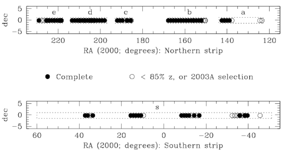
Figure 1: The location of the 2SLAQ Input Catalogue (dotted rectangles) and observered fields (circles). Solid circles indicate fully observed fields with high, $\geq 85\%$ overall completeness, while hollow circles have less than 85% overall completeness or fields with non-standard selection criteria.

2.1 The 2dF-SDSS LRG And QSO Survey

A full description of the 2SLAQ Survey can be found in Cannon et al. (2006). At its heart, the 2SLAQ Survey relies on the SDSS photometric survey to supply LRG targets for spectroscopic follow-up using the 2 Degree Field (2dF) instrument on the Anglo-Australian Telescope (AAT).

The selection of distant ($z>$ 0.4) LRGs is done on the basis of SDSS $gri$ photometric data, using the ($g-r$) versus ($r-i$) colours and the SDSS “de Vaucouleurs” $i$-band magnitude. The criteria are similar to those used for the faint “Cut II” sample in the SDSS LRGs (Eisenstein et al., 2001) and are described in detail by Cannon et al. (2006). (See Fukugita et al. (1996) for a description of the SDSS filters.)

The survey covers two narrow stripes along the celestial equator ($|$$\delta$$|$ $<$ 1.5^∘). The Northern Stripe runs from $8\aas@@fstack{h}4$ to $15\aas@@fstack{h}3$ in Right Ascension and is broken into 5 sub-stripes to utilise the best photometric data. The Southern Stripe runs from $20\aas@@fstack{h}6$ to $4\aas@@fstack{h}0$. Figure 1 shows the layout of the target stripes and the 2dF fields observed. The total area of the survey, including the overlap regions, was approximately 180 degrees². Again, complete details of the Survey fields are given by Cannon et al. (2006).

It is important to be aware of the tiling strategy of the 2SLAQ survey when estimating the clustering of the LRGs. A simpler tiling scheme was used for 2SLAQ than for the preceding 2dFGRS/2QZ survey. For instance, for 2SLAQ, the 2dF tiles were offset by 1.2 deg in the RA direction as opposed to a variable spacing strategy employed by the 2dFGRS and 2QZ. Again, contrary to the 2dFGRS/2QZ, the galaxies in 2SLAQ were given higher fibre assignment priority, with the LRGs always having priority over the QSOs. This makes sure the LRG selection was not biased by the QSOs. The details of the survey mask and selection function will be described in detail in Section 2.3.

The total 2SLAQ LRG dataset consists of a total of 18 487 spectra for 14 978 discrete objects; 13 784 of these (92%) have reliable, “Qop” $\geq 3$ redshifts. From these “Qop”$\geq 3$ objects, 663 are identified as being stars, leaving a total of 13 121 galaxies.

We cut this sample down further by using only those confirmed LRGs which were part of the top priority “Sample 8” selection as described fully in Cannon et al. (2006). These galaxies comprise the most rigorously defined 2SLAQ LRG sample where completeness is highest due to their top priority for spectroscopic observation. The exact Sample 8 selection lines in the $gri$ plane are shown in Fig. 1 of Cannon et al (2006). The magnitude limits is $i_{deV}<$ 19.8 (de-reddened). However, the sample we use does include observations taken in the 2003A semester, where a brighter $i_{deV}<$ 19.5 magnitude limit was used, as long as the observed LRG would have made the “Sample 8” selection. We do not include observations taken from fields a01, a02 and s01 (see Cannon et al. (2006)) as they have low completeness and should not be used in statistical analyses. Once the final selection criteria had been decided, there were 25 795 “Sample 8” LRG targets at a sky density of about 70 per square degree. Approximately 40% (10 072) of these objects were observed, with 9 307 obtaining “Qop”$\geq 3$. After imposing the cuts above, this leaves a total of 8 656 LRGs, 5 995 in the Northern Galactic Stripe and 2 661 in the Southern Galactic Stripe. For all further analysis, this is the sample utilised which we call the “Gold Sample” and has a $\bar{z}_{Gold}$ = 0.55.

Sample Description	Number in sample	North	South
Unique Objects	14 978	10 369	4 609
“Qop” $\geq$ 3	13 784	9 726	4 058
M Stars	663
LRGs	13 121	9 280	3 841
LRG Sample 8	8 756	6 076	2 680
excl. a01, a02, s01	8 656	5 995	2 661

Table 1: The 2SLAQ LRG Survey; Numbers of different Samples. Over 18 000 spectra were obtained, resulting in 13 121 spectroscopically confirmed Luminous Red Galaxies. We use the LRGs with the “Sample 8” Input Priority settings for our analysis but do not include the data taken in the a01, a02 and s01 fields which have low redshift completeness and should be excluded from statistical analysis (Cannon et al., 2006). Thus we are left with 8 656 in our “Gold Sample”.

2.2 The Two-Point Correlation Function

Here we give a brief description of the 2-point correlation function (2PCF); for a more formal treatment the reader is referred to Peebles (1980) which presents the basis for the rest of the section. To denote the redshift-space (or $z$-space) correlation function, we will use the notation $\xi(s)$ and to denote the real-space correlation function, $\xi(r)$ will be used, where $s$ is the redshift-space separation of two galaxies and $r$ is the real-space separation.

The 2-point correlation function, $\xi(x)$, is defined by the joint probability that two galaxies are found in the two volume elements $dV_{1}$ and $dV_{2}$ placed at separation $x$,

$$dP_{12}=n^{2}[1+\xi(x)]\,dV_{1}dV_{2}.$$ (1)

To calculate $\xi(x)$, $N$ points are given inside a window $W$ of observation, which is a three-dimensional body of volume $V(W)$. An estimation of $\xi(x)$ is based on an average of the counts of neighbours of galaxies at a given scale, or more precisely, within a narrow interval of scales. An extensively used estimator is that of Davis & Peebles (1983) and is usually called the standard estimator,

$$\xi_{Std}(s)=\left(\frac{N_{rd}}{N}\frac{DD(s)}{DR(s)}\right)-1$$ (2)

where $DD(s)$ is the number of pairs in a given catalogue (within the window $W$) and $DR(s)$ is the number of pairs between the data and the random sample with separation in the same interval. $N_{rd}$ is the total number of random points and $N$ is the total number of data points. A value of $\xi$ = 1 implies there are twice as many pairs of galaxies than expected for a random distribution and the scale at which this is the case is called the correlation length.

2.3 Constructing a random catalogue and survey Completeness

The two point correlation function, $\xi$, is measured by comparing the actual galaxy distribution to a catalogue of randomly distributed galaxies. Following the method of Hawkins et al. (2003) and Ratcliffe et al. (1998), these randomly distributed galaxies are subject to the same redshift, magnitude and mask constraints as the real data and we modulate the surface density of points in the random catalogue to follow the completeness variations. We now look at the various factors this involves.

Following Croom et al. (2004), we discuss issues regarding the 2SLAQ Survey completeness. As with the rest of the paper, we are only concentrating on the properties of the luminous red galaxies. One might think the parallel 2SLAQ QSO survey would have a bearing on subsequent discussion but due to the higher priority given to the fibres assigned to observe the LRGs, the QSO Survey has no impact on LRG clustering considerations, as already noted. For more description of the clustering of the QSOs the reader is referred to da Angela et al. (2006).

Three main, separate types of completeness are going to be considered; i) Coverage completeness, $f_{c}$, which we define as the fraction of the Input 2SLAQ catalogue sources that have spectroscopic observations. Identically to Croom et al. (2004), we calculate $f_{c}$, as being the ratio of observed to total sources in each of the sectors defined by overlapping 2SLAQ fields, which are pixelized on 1 (one) arcminute scales; ii) Spectroscopic completeness, $f_{s}$ which can be said to be the fraction of observed objects which have a certain spectroscopic quality; iii) Incompleteness due to fibre collisions which is dealt with separately from coverage completeness

For coverage completeness and spectroscopic completeness we assume that both are functions of angular position only, i.e. $f_{c}(\theta)$ and $f_{s}(\theta)$ respectively. The spectroscopic (i.e. redshift) completeness does depend on magnitude but this is not relevant for any of the purposes of this paper.

2.3.1 Angular $+$ Spectroscopic Completeness and Fibre Collisions

There are various technical details associated with the 2dF instrument. Variations in target density, the small number of broken or otherwise unuseable fibres and constraints owing to the minimum fibre placing (see below) could introduce false signal into the clustering pattern. For our analysis, the 2SLAQ survey consists of 80 field pointings. Many of these pointings overlap, alleviating some of these technical issues.

The design of the 2dF instrument means that fibres cannot be placed closer than approximately 30 arcsec (Lewis et al., 2002) so both members of a close pair of galaxies cannot be targeted in a single fibre configuration. The simple, fixed-spacing tiling strategy of the 2SLAQ Survey means that not all such close pairs are lost. Neighbouring tiles have significant areas of overlap and much of the survey sky area is targeted more than once. This allows us to target both galaxies in some close pairs. Nevertheless, the survey misses a noticeable fraction of close pairs. It is important to assess the impact of this omission on the measurement of galaxy clustering and to investigate schemes that can compensate for the loss of close pairs.

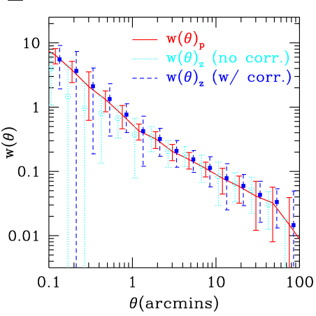
Figure 2: The $w(\theta)$ for the 2SLAQ redshift catalogue (light blue) dotted, open circles compared to the parent catalogue solid (red) line. The errors quoted are “Field-to-field” errors with the sub-areas used given by Table 2. The filled blue squares, with dashed error bars, show the $w(\theta)$ from the redshift catalogue after the correction for fibre collisions has been applied. The values for the uncorrected (corrected) $w(\theta)$ from the redshift catalogue have been moved by $\Delta\log=-(+)0.05$ in the abscissa for clarity. Note also that the solid line represents the filled squares given in Figure 5.

To quantify the effect of these so-called ‘fibre collisions’ we have followed previous 2dF studies (e.g. Hawkins et al., 2003; Croom et al., 2004) and calculated the angular correlation function for galaxies in the 2SLAQ parent catalogue, $w_{p}(\theta)$, and for galaxies with redshifts used in our $\xi$ analysis, $w_{z}(\theta)$. We used the same mask to determine the angular selection for each sample.

As shown in Figure 2, on scales $\theta\;\lower 3.22916pt\hbox{$\sim$}\hbox to0.0pt{\hss\raise 1.1625pt\hbox{$>$}}\;3^{\prime}$, the angular correlations of the Parent and Redshift catalogue are very nearly consistent. At scales $\theta\;\lower 3.22916pt\hbox{$\sim$}\hbox to0.0pt{\hss\raise 1.1625pt\hbox{$<$}}\;2^{\prime}$, we begin to lose close pairs. To correct for this effect, we use a similar method to Hawkins et al. (2003) and Li et al. (2006). The quantity $w_{\rm cor}(\theta)=(1+w_{p})/(1+w_{z})$ is used to weight our 3-D DD pairs. For each DD pair, the angular separation on the sky is calculated and the galaxy-galaxy pair is weighted by the $w_{\rm cor}(\theta)$ ratio given by the relevant angular separation. The result of weighting by this factor, is shown by the filled (dark blue) squares in Fig. 2.

The last stage in determining the angular “mask” is to evaluate the spectroscopic completeness of the survey, $f_{s}(\theta)$ which for our purposes, we again assume depends on sky position only. This function essentially describes the success rate in obtaining a spectrum and reliable redshift for a given fibred object. Here the advantage of LRGs becomes apparent. With their well-defined early-type spectra and often very strong Ca H+K break around 4000Å, a high success rate was achieved when calculating a redshift for the 2SLAQ LRG objects. Also, it became apparent that our 4 hour per field exposure time was on occasion generous and relatively high S/N spectra were recorded. The spectroscopic completeness has been estimated at 94.5 per cent for the primary “Sample 8” and the redshift completeness at 96.7 per cent, giving an overall completeness of 91.4 per cent (Cannon et al. 2006, Section 5.5, Figure 5).

2.3.2 Radial Selection Function and Estimates of the LRG $N(z)$

The observed distribution of galaxy redshifts is given in Figure 3. Plotted are the $N(z)$ distributions, binned into redshift slices of $\Delta z$=0.02, for the “Gold Sample”. Also shown is a polynomial fit (7th order) to the $N(z)$ distribution, which is used to generate the random distributions. Checking the $N(z)$ fits using higher order polynomials or convolved double Gaussians does not give tighter reproduction of the observed LRG redshift distribution.

Combining the radial selection function and the completeness map, we generate a random catalogue of points which we now use to calculate the LRG correlation function.

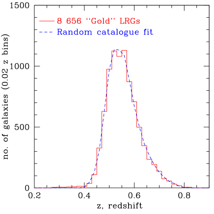
Figure 3: The redshift distribution for the 2SLAQ LRG “Gold” Sample we use. The solid red histogram is for the “Gold” Sample. The dashed blue line is from the normalised random catalogue.

2.4 Calculating the 2-point Correlation Function

As the LRG correlation function, $\xi(s)$, probes high redshifts and large scales, the measured values are highly dependent on the assumed cosmology. In determining the comoving separation of pairs of LRGs we choose to calculate $\xi(s)$ for two representative cosmological models. The first uses the cosmological parameters derived from WMAP, 2dFGRS and other data (Spergel et al., 2003, 2006; Percival et al., 2002; Cole et al., 2005; Sánchez et al., 2006) with $(\Omega_{\rm m}$,$\Omega_{\Lambda})=$ $(0.3,0.7)$, which we will call the $\Lambda$ cosmology. The second model assumed is an Einstein-de Sitter cosmology with $(\Omega_{\rm m}$,$\Omega_{\Lambda})=$ $(1.0,0.0)$ which we denote as the EdS cosmology. We will quote distances in terms of $~{}h^{-1}~{}{\rm Mpc}$, where $h$ is the dimensionless Hubble constant such that $H_{0}=100h{\rm~{}km~{}s}^{-1}~{}{\rm Mpc}^{-1}$.

We have used the minimum variance estimator suggested by Landy & Szalay (1993) to calculate $\xi(s)$. Using notation from Martínez & Saar (2002), this estimator is

$$\xi_{\mathrm{LS}}(s) = 1+\left(\frac{N_{rd}}{N}\right)^{2}\frac{DD(s)}{RR(s)}-2\left(\frac{N_{rd}}{N}\right)\frac{DR(s)}{RR(s)}$$ (3)

$$\equiv \frac{\langle DD\rangle-\langle 2DR\rangle+\langle RR\rangle}{\langle RR\rangle},$$ (4)

where the angle brackets denote the suitably normalised LRG-LRG, LRG-random and random-random pairs counted at separation $s$. We use bin widths of $\delta\log(s/\;h^{-1}{\rm Mpc})$ = 0.1. The density of random points used was 20 times the density of LRGs. The Hamilton estimator is also utilised (Hamilton, 1993) where

$$\xi_{\mathrm{Ham}}(s)=\frac{DD(s)\cdot RR(s)}{DR(s)^{2}}-1$$ (5)

and no normalisation is required. Since we find the differences of the Hamilton estimator compared to the Landy-Szalay method are negligible, the Landy-Szalay method is quoted in all $\xi(s)$ figures unless explicitly stated otherwise.

Three methods are employed to estimate the likely errors on our measurements. The first is a calculation of the error on $\xi(s)$ using the Poisson estimate of

$$\sigma_{\mathrm{Poi}}(s)=\frac{1+\xi(s)}{\sqrt{DD(s)}}.$$ (6)

The second error estimate method is what we shall call the field-to-field errors, calculated by

$$\sigma_{\mathrm{FtF}}^{2}(s)=\frac{1}{N-1}\sum_{i=1}^{N}\frac{DR_{i}(s)}{{DR(s)}}[\xi_{i}(s)-\xi(s)]^{2}$$ (7)

where $N$ is the total number of subsamples i.e. “the fields” and $\xi_{i}(s)$ is from one field. $\xi(s)$ is the value for $\xi$ from the entire sample and is not the mean of the subsamples. For our studies the natural unit of the “Field-to-field” (FtF) subsample is given by the area geometry covered by the survey. Thus we take $N=9$, and split the NGP area into five regions, a,b,c,d,e and the SGP in to four regions, named s06, s25, s48, s67. Details of the FtF subsamples are given in Table 2.

The third method is usually referred to as the jackknife estimate, and has been used in other correlation studies (e.g. Scranton et al., 2002; Zehavi et al., 2002; Zehavi et al., 2005). Here we estimate $\sigma$ as

$$\sigma_{\mathrm{Jack}}^{2}(s)=\sum_{i^{\prime}=1}^{N}\frac{DR_{i^{\prime}}(s)}{{DR(s)}}[\xi_{i^{\prime}}(s)-\xi(s)]^{2}$$ (8)

where $i^{\prime}$ is used to signify the fact that each time we calculate a value of $\xi(s)$, all subsamples are used bar one. For the jackknife errors, we divide the survey into 32 approximately equal sized areas, leaving out $\sim$4.5 square degrees from the entire survey area at one time. Thus a jackknife subsample will contain $\sim$8,350 LRGs. We can then work out the covariance matrix in the traditional way,

$${\rm Cov}(\xi_{i},\xi_{j})=\frac{N-1}{N}\,\sum_{l=1}^{N}\,(\xi_{i}^{l}-\bar{\xi}_{i}^{l})\,(\xi_{j}^{l}-\bar{\xi}_{j}^{l})$$ (9)

where $\bar{\xi}$ is the mean value of $\xi$ measured from all the jackknife subsamples and $N=32$ in our case (c.f. Zehavi et al. (2002)). The variances are obtained from the leading diagonal elements of the covariance matrix,

$$\sigma_{i}^{2}={\rm Cov}(\xi_{i},\xi_{i})$$ (10)

When examing the covariance matrix, we find the measurements to be slightly noisy as well as an indication of anti-correlation (contrary to theoretical expectations). However, we note that in the other recent clustering studies, noisy covariances and anti-correlations were also noted (e.g. Scranton et al., 2002; Zehavi et al., 2002; Zehavi et al., 2005).

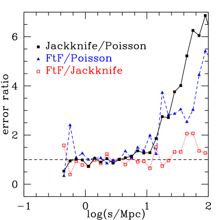
Figure 4: The ratio of Poisson to jackknife errors (solid black line and squares), Poisson to ‘field-to-field’ errors, (dashed blue line and triangles) and ‘field-to-field’ to jackknife errors (dotted red line and open squares). As can be seen, all error estimators are comparable on scales $\lesssim 10\;h^{-1}{\rm Mpc}$, while at larger scales than this the jackknife and ‘field-to-field’ errors are considerably larger than the simple Poisson estimates. The magnitude of the ‘field-to-field’ and jackknife errors are very similar from the smallest scales considered here up to $\approx 40\;h^{-1}{\rm Mpc}$.

The ratio of Poisson to jackknife errors, Poisson to ‘field-to-field’ errors, and the ‘field-to-field’ to jackknife errors are given in Figure 4. As can be seen, all error estimators are comparable on scales $\lesssim 10\;h^{-1}{\rm Mpc}$, while at larger scales than this the jackknife and ‘field-to-field’ errors are considerably larger than the simple Poisson estimates. The magnitude of the ‘field-to-field’ and jackknife errors are very similar from the smallest scales considered here, up to $\approx 40\;h^{-1}{\rm Mpc}$. This behaviour has been noted in other correlation function work, e.g. da Ângela et al. (2005). We also note that field-to-field and jackknife errors are more comparable in size, regardless of scale. Hence, the errors that are quoted on all correlation functions from here on are the square roots of the variances from the jackknife method, except for the case of the angular correlation function, $w(\theta)$, where we quote the “Field-to-field” error.

Area Name	RA(J2000) range/∘	LRGs	Randoms	$\rho_{rd}/\rho_{LRG}$
a	123.0 - 144.0	617	10 745	17.41
b	150.0 - 168.0	1 837	35 449	19.30
c	185.0 - 193.0	572	14 484	25.32
d	197.0 - 214.0	1 723	34 373	19.95
e	218.0 - 230.0	1 246	24 849	19.94
s06	309.2 - 330.0	745	12 457	16.72
s25	330.0 - 360.0	876	18 499	21.12
s48	0.0 - 30.0	658	13 516	20.54
s67	30.0 - 59.7	382	8 749	22.90
Entire Survey		8 656	173 120	20.00

Table 2: The 2SLAQ LRG Survey; Names and Right Ascension ranges for the $N=9$ sections used when calculating the field-to-field errors.

2.5 Measuring $\xi(\sigma,\pi)$

Having described how we calculate galaxy-galaxy separations in redshift-space in order to measure $\xi(s)$, we can now study the clustering perpendicular, $\sigma$, and parallel, $\pi$, to the line of sight. We work out the co-moving distance, $r_{c}$, to our object, which is equal to the distance parallel to the line of sight i.e. a $\pi$ value. Thus, already knowing the redshift-space separation, s, we can use

$$s^{2}=\sigma^{2}+\pi^{2}$$ (11)

to find $\sigma$. At this point it should be noted that $\sigma$ is sometimes designated by $r_{p}$, where $r_{p}\equiv\sigma$. For this paper we shall continue to use $\sigma$ for the perpendicular separation. Closely following Hoyle et al. (2002), $\xi(\sigma,\pi)$ can be estimated in a similar way to $\xi(s)$. A catalogue of points, that have the same radial selection function and angular mask as the data but are unclustered, is used to estimate the effective volume of each bin. As stated above, the unclustered, random catalogue also contains 20 times more points than the data. The $DD(\sigma,\pi)$, $DR(\sigma,\pi)$ and the $RR(\sigma,\pi)$, where again $D$ stands for data LRG and $R$ stands for random, counts in each $\sigma$ and $\pi$ bins are found and the Landy-Szalay estimator

$$\xi_{LS}(\sigma,\pi)=\frac{\langle DD(\sigma,\pi)\rangle-\langle 2DR(\sigma,\pi)\rangle+\langle RR(\sigma,\pi)\rangle}{\langle RR(\sigma,\pi)\rangle},$$ (12)

is used to find $\xi(\sigma,\pi)$, with bins of $\delta\log(\sigma/\;h^{-1}{\rm Mpc})=\delta\log(\pi/\;h^{-1}{\rm Mpc})=0.2$. Again, we compute three types of errors to use as a guide; Poisson, “Field-to-field” and Jackknife errors are calculated for $\xi(\sigma,\pi)$ as in equations 6 to 8. Again, after comparing the different $\xi(\sigma,\pi)$ error estimators we find that on the scales we are considering, the jackknife error is sufficient for our purposes.

2.6 The Projected Correlation Function, $w_{p}(\sigma)$

Although we are now in a position to calculate the redshift-space correlation function, the real-space correlation function, $\xi(r)$, which measures the physical clustering of galaxies and is independent of redshift-space distortions, remains unknown. However, due to the fact that redshift distortion effects only appear in the radial component, by integrating along the $\pi$ direction, we can calculate the projected correlation function,

$$w_{p}(\sigma)\;\;=2\int_{0}^{\infty}\xi(\sigma,\pi)d\pi$$ (13)

In practice we set the upper limit on the integral to be $\pi_{\rm max}=70~{}h^{-1}~{}{\rm Mpc}$ as at this large-scale, the effect of clustering is negligible, while linear theory should also apply. The effect of $z$-space distortions due to small-scale peculiar velocities or redshift errors is also minimal on this scale. Changing the value of $\pi_{\rm max}$ from $25~{}h^{-1}~{}{\rm Mpc}$ to $100~{}h^{-1}~{}{\rm Mpc}$ makes negligible difference in the result.

Due to $w_{p}(\sigma)$ now describing the real-space clustering, the integral in Equation 13 can be re-written in terms of $\xi(r)$, (Davis & Peebles, 1983)

$$w_{p}(\sigma)=2\int_{\sigma}^{\pi_{\rm max}}\frac{r\,\xi(r)}{\sqrt{(r^{2}\,-\,\sigma^{2})}}dr.$$ (14)

If we then assume that $\xi(r)$ is a power-law of the form, $\xi(r)\,=\,(r/r_{0})^{-\gamma}$, equation 14 can be integrated analytically such that

$$\frac{w_{p}(\sigma)}{\sigma}=\left(\frac{r_{0}}{\sigma}\right)^{\gamma}\left[\frac{\Gamma(\frac{1}{2})\,\Gamma(\frac{\gamma-1}{2})}{\Gamma(\frac{\gamma}{2})}\right]=\left(\frac{r_{0}}{\sigma}\right)^{\gamma}A(\gamma)$$ (15)

where $A(\gamma)$ represents the quantity inside the square brackets and $\Gamma(x)$ is the Gamma function calculated at $x$. We now have a method for calculating the real-space correlation length and power-law slope, denoted $r_{0}$ and $\gamma$ respectively.

2.7 The Real-space Correlation Function, $\xi(r)$

Using the projected correlation function, $w_{p}(\sigma)$, it is now possible to find the $r_{0}$ and $\gamma$ for the real-space correlation function. However, if one does not assume a power-law $\xi(r)$, it is still possible to estimate $\xi(r)$ by directly inverting $w_{p}(\sigma)$. Following Saunders et al. (1992) we can write

$$\xi(r)=-\frac{1}{\pi}\int^{\infty}_{r}\frac{(dw(\sigma)/d\sigma)}{(\sigma^{2}-r^{2})^{\frac{1}{2}}}d\sigma.$$ (16)

Assuming a step function for $w_{p}(\sigma)=w_{i}$ in bins centred on $\sigma_{i}$, and interpolating between values,

$$\xi(\sigma_{i})=-\frac{1}{\pi}\sum_{j\geq i}\frac{w_{j+1}-w_{j}}{\sigma_{j+1}-\sigma_{j}}\ln\left(\frac{\sigma_{j+1}+\sqrt{\sigma^{2}_{j+1}-\sigma^{2}_{i}}}{\sigma_{j}+\sqrt{\sigma^{2}_{j}-\sigma^{2}_{i}}}\right)$$ (17)

for $r=\sigma_{i}$. We shall be utilising this interpolation method to check whether a power-law description is valid for our 2SLAQ Survey data and, if so, what values the parameters $r_{0}$ and $\gamma$ take.

3 Results

3.1 The LRG Angular Correlation Function, $w(\theta)$

We first analyse the form of the angular correlation function, $w(\theta)$. The full input catalogue contains approximately 75 000 LRGs mainly from areas in the two equatorial stripes; about 40% of this area was observed spectroscopically. As stated in Section 2, approximately a third of the objects in the total input catalogue pass the Sample 8 selection criteria. As well as providing estimates of fibre collision and other angular incompletenesses, the angular function is of interest in itself, particularly given the narrow redshift range from which the sample is derived. We use 25 795 “Sample 8” LRG targets to estimate the $w(\theta)$. We first note that the function gives clear indication of a change of slope at $\theta=2$ arcmin or $\approx 1\;h^{-1}{\rm Mpc}$ in the $\Lambda$ cosmology. Considering the form of $w(\theta)=A\theta^{1-\gamma}$, at $\theta<2$ arcmin the slope is $\gamma=-2.17\pm{0.07}$ and at larger scales the slope is $\gamma=-1.67\pm{0.07}$. Using Limber’s formula from Phillipps et al. (1978) and assuming a double power-law form where the slope changed between -2.17 and -1.67 at $\sim 1.5\;h^{-1}{\rm Mpc}$ (comoving), we found in the $\Lambda$ case, a value of $r_{0}=4.85\pm 0.3\;h^{-1}{\rm Mpc}$ at small scales and $r_{0}=6.89\pm 0.6\;h^{-1}{\rm Mpc}$ at large scales (see Fig. 5). We shall check models of this form against the deprojected correlation function $\xi(r)$ (see Figure 9 below). We find that the form of this double power-law gives reasonable fits to the data in the LRG redshift survey, although the large scale slope derived from the input catalogue $w(\theta)$ appears slightly flatter than in the semi-projected and 3-D correlation functions (see below). The reason for this is not clear, although it could be that $w(\theta)$ is more sensitive to any artificial gradient in the LRG data. Thus, we checked for an angular systematic in the data by calculating the angular correlation between spectroscopic LRGs that are not at the same redshift. We find this is consistent with zero and so such systematics do not explain the flatter slope for $w(\theta)$ at large-scales. The most likely explanation is the different fitting ranges for $w(\theta)$ and the semi-projected correlation function. This test also suggests that the upturn at $\theta<2$ arcmins is a real feature. It will be seen that $w(\theta)$ gives the strongest evidence of all the correlation function statistics for non-power-law behaviour in $\xi(r)$. A similar feature is seen by Zehavi et al in the SDSS MAIN galaxy sample and to a lesser extent in the SDSS LRG survey. Reports of such features in galaxy correlation functions go back to Shanks et al. (1983). We simply report the existence of this feature in the LRG data and leave further interpretation for a future paper. Possible interpretations could include models of halo occupation distributions (HOD) in the standard model case or the possibility that it might represent a real feature in the mass distribution in the case of other models. We also show results from White et al. (2007, open, black circles, Figure 5) who report on the angular correlation function as a route to estimating merger rates of massive red galaxies. As can be seen, these measurements from the NOAO Deep Wide-Field Survey (NDWFS; Jannuzi & Dey, 1999) agree very well with the 2SLAQ LRG results, though as we shall discuss later, care always has to be taken when comparing measurements from galaxy surveys with different selections.

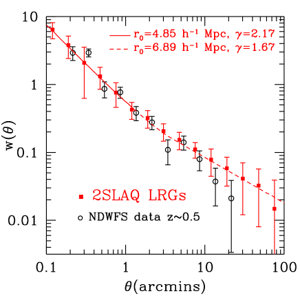
Figure 5: The angular correlation function, $w(\theta)$ from the 2SLAQ input catalogue containing 25 795 LRG targets (solid, red squares). Clear evidence is seen for a change of power-law slope on $\sim 2$arcmin scales which is equivalent to $\approx 1\;h^{-1}{\rm Mpc}$. The open (black) circles show the results from the NDWFS at $z\sim 0.5$ (White et al., 2007).

3.2 The LRG Redshift-Space Correlation Function, $\xi(s)$

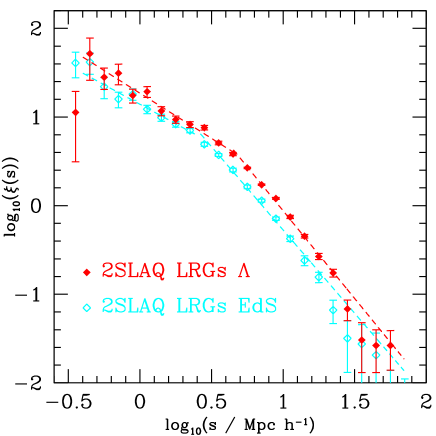
Figure 6: The redshift-space 2-point correlation function, $\xi(s)$ for the 2SLAQ LRG Survey in a $\Lambda$ cosmology (filled, red diamonds) and an Einstein-de Sitter, $\Omega_{\rm m}=1$, cosmology (open, cyan diamonds). The dashed lines shown are the double power-law best-fit models to data with the associated values of $s_{0}$ and $\gamma$ given in Table 3.

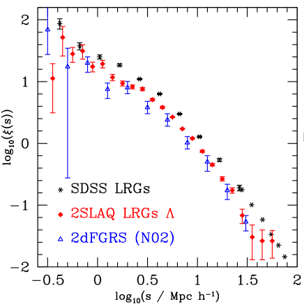
Figure 7: The redshift-space correlation function, $\xi(s)$ for the 2SLAQ LRG Survey (filled, red, diamonds). For comparison, data from the SDSS LRG Survey (black stars Zehavi et al., 2005; Eisenstein et al., 2005) and the high luminosity early-type 2dFGRS, (Norberg et al., 2002, open blue triangles) are also plotted.

Using the above corrections including that for fibre collisions, the 2SLAQ LRG redshift-space 2PCF, $\xi(s)$, is shown in Figure 6. There is clear evidence for downturns at small scales $\lower 3.22916pt\hbox{$\sim$}\hbox to0.0pt{\hss\raise 1.1625pt\hbox{$<$}}2.5\;h^{-1}{\rm Mpc}$ and large scales $\lower 3.22916pt\hbox{$\sim$}\hbox to0.0pt{\hss\raise 1.1625pt\hbox{$>$}}10\;h^{-1}{\rm Mpc}$ that are not described well by a single power-law. This turn-over is consistent with the redshift-space distortion effects one would expect in a $\xi(s)$ correlation function - namely the “Finger of God” effect at small scales due to intrinsic velocity dispersions and large-scale flattening from peculiar motions due to coherent cluster in-fall. However, we note that real features in the real-space correlation function, $\xi(r)$, may also be contributing. We have also estimated the effect of the integral constraint ($IC$, Peebles, 1980) at larger scales. Using our global (N$+$S) normalisation of the correlation function, we assume a total number of 8 656 galaxies in a total volume of $4.5\times 10^{7}\;h^{-1}{\rm Mpc}^{3}$ and $r_{0}=7.45\;h^{-1}{\rm Mpc}$. Integrating with a $\gamma=1.8$ power-law to 20$\;h^{-1}{\rm Mpc}$ gives an $IC=3.5\times 10^{-4}$ and to 100$\;h^{-1}{\rm Mpc}$, an $IC=2.4\times 10^{-3}$. Adding such contributions would make negligible contributions to any of our correlation function fits.

We now attempt to parameterise the $\xi(s)$ data. The simplest model traditionally fitted to correlation function estimates is a power law of the form

$$\xi(s)=\left(\frac{s}{s_{0}}\right)^{-\gamma},$$ (18)

where $s_{0}$ is the comoving correlation length, in units of $\;h^{-1}{\rm Mpc}$. However, with the redshift-space distortion effects being so evident, we find that a single-power is insufficient to describe the data and thus switch to a double power-law model

$$\xi(s)=\left\{\begin{array}[]{ll}\left(\frac{s}{s_{1}}\right)^{\gamma_{1}}&s\leq s_{\rm{b}}\;\;\;\rm{and}\\ \left(\frac{s}{s_{2}}\right)^{\gamma_{2}}&s>s_{\rm{b}}\end{array}\right.$$ (19)

where $s_{\rm b}$ is the scale of the “break” from one power-law description to the other. This $\xi(s)$ model is used later in Section 4. We fit the double power-law continuously over the range $0.4<s<60\;h^{-1}{\rm Mpc}$. We fix the break-scale at 4.5$\;h^{-1}{\rm Mpc}$ for the $\Lambda$ cosmology and at 2.5$\;h^{-1}{\rm Mpc}$ for the EdS cosmology. We perform a $\chi^{2}$-fit, following the prescription given by Press et al. (1992, Chap. 15), to find the best-fit values for $s_{1},\gamma_{1},s_{2},$ and $\gamma_{2}$. We plot the best fit double-power law models in Figure 6 and quote the values of $s_{1},\gamma_{1},s_{2},$ and $\gamma_{2}$, in Table 3. The errors quoted in Table 3 are only indicative because no account has been taken of the non-independence of the correlation function points in deriving the $\xi(s)$ fits.

Table 3: Values of the redshift-space correlation length and slope for the 2SLAQ LRG Survey from $\xi(s)$. When a $\Lambda$ cosmology was assumed, $s_{b}$ was set at 4.5$\;h^{-1}{\rm Mpc}$. When a EdS cosmology was assumed, $s_{b}$ was set at 2.5 $\;h^{-1}{\rm Mpc}$.

$\Lambda$	$s_{0}<4.5\;h^{-1}{\rm Mpc}$	$s_{0}>4.5\;h^{-1}{\rm Mpc}$
${\rm s}_{0}/\;h^{-1}{\rm Mpc}$	$17.3^{+2.5}_{-2.0}$	$9.40\pm 0.19$
$\gamma$	$1.03\pm 0.07$	$2.02\pm 0.07$
$\chi^{2}_{min}$ (reduced)	1.95	1.88
EdS	$s_{0}<2.5\;h^{-1}{\rm Mpc}$	$s_{0}>2.5\;h^{-1}{\rm Mpc}$
${\rm s}_{0}/\;h^{-1}{\rm Mpc}$	$20.3^{+9.4}_{-5.0}$	$7.15\pm 0.13$
$\gamma$	$0.88\pm 0.11$	$1.88^{+0.05}_{-0.04}$
$\chi^{2}_{min}$ (reduced)	0.91	3.43

For comparison, in Figure 7 results from the SDSS LRG study are reported (Zehavi et al., 2005; Eisenstein et al., 2005) as well as selected measurements from the 2dFGRS (Norberg et al., 2002). The 2dFGRS is a blue, $b_{J}$ selected survey of generally $\sim L^{*}$ galaxies. However, in Norberg et al. (2002), the sample is segregated by luminosity and spectral type, the latter governed by the $\eta$ parameter (Madgwick et al., 2003). Assuming a conversion of $M^{0.2}_{r}-M_{b_{\rm J}}\simeq-1.1$, we calculate that the faintest 2SLAQ LRGs in our sample have an $M_{b_{\rm J}}\approx-20.5$. Weighting according to number, we thus use the Norberg et al. (2002) $-21.00>M_{b_{\rm J}}-5\log h>-22.00$ and $-20.50>M_{b_{\rm J}}-5\log h>-21.50$ luminosity ranges from their “early-type” volume-limited sample. This is shown by the (blue) open triangles in Figure 7.

The 2SLAQ LRG measurement is lower than the SDSS LRG result. It should not be concluded that this is evidence of evolution because although the SDSS survey is at a lower mean redshift, it was designed in order to target generally redder, more luminous LRGs (Eisenstein et al., 2001). The 2SLAQ LRG colour selection criteria is relatively relaxed for an “LRG” survey, leading to bluer and less luminous galaxies making it into our sample. We note here that it is non-trival comparing clustering amplitudes and bias strengths for surveys with (sometimes very) different colour/magnitude/redshift selections. As such, a more detailed analysis of the clustering evolution for SDSS and 2SLAQ LRGs is presented in Wake et al. (2007, in prep.).

The 2dFGRS $M_{b_{\rm J}}<-20.5$, early-type sample is at least approximately matched in terms of luminosity to the 2SLAQ LRGs. Once we have determined the linear bias parameter $b$ for the $z=0.55$ 2SLAQ LRGs, we shall be able to use a simple model of bias evolution, to compare these low redshift 2dFGRS and 2SLAQ LRG results.

3.3 The Projected Correlation function, $w_{p}(\sigma)$

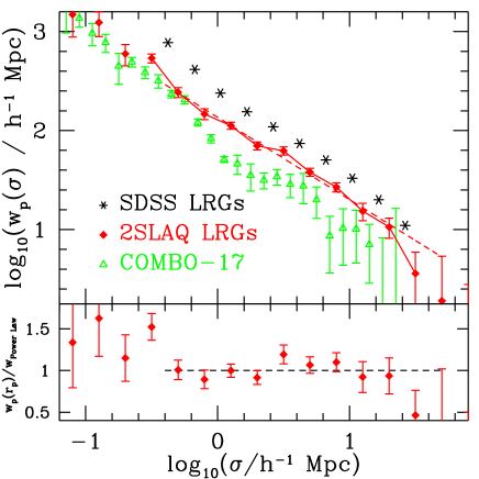
Figure 8: The 2SLAQ LRG projected correlation function, $w_{p}(\sigma)$, with errorbars from the “Jackknife” estimates (solid, red diamonds). The dashed line is the power-law that gives the best fitting line from the $\chi^{2}$ analysis (see Table 4). The measurements from the SDSS LRGs (Zehavi et al., 2005) are shown as a guide, with the SDSS errors being of comparable size to the plotted stars. The open (green) triangles are from COMBO-17 Red Sequence (Phleps et al., 2006). The lower panel shows the 2SLAQ LRG $w_{p}(\sigma)$ measurements divided by this best-fitting power law with the dashed line covering $0.4<\sigma<50\;h^{-1}{\rm Mpc}$.

Again, after applying coverage, spectroscopic and fibre collision corrections, the projected correlation function, $w_{p}(\sigma)$, is presented in Figure 8. We again fit a single power-law to the 2SLAQ data and find that for the $\Lambda$ cosmology, a single power-law is an adequate description, returning a reduced $\chi^{2}$ = 1.17 over $0.4<\sigma<50\;h^{-1}{\rm Mpc}$. Over the wider range of $0.1<\sigma<50\;h^{-1}{\rm Mpc}$, the $\chi^{2}$ increases to 1.71. Thus the projected correlation function appears to deviate from a single power law at small scales in the way described in Section 3.1. The results for $r_{0}$ and $\gamma$ assuming a single power-law are given in Table 4. The errors are taken from jack-knife estimates found by dividing the survey into 32 subareas.

Table 4: Values of the projected correlation function, $w_{p}(\sigma)$, correlation length and slope for the 2SLAQ LRG Survey. In the $\Lambda$ model, fits were performed over the range $0.4<\sigma<50.0\;h^{-1}{\rm Mpc}$, whereas for the EdS model, fits were performed over $0.25<\sigma<40.0\;h^{-1}{\rm Mpc}$. The value of $r_{0}$ was found using equation 15.

	$\Lambda$	EdS
$r_{0}/\;h^{-1}{\rm Mpc}$	$7.30\pm 0.34$	$5.40\pm 0.31$
$\gamma$	$1.83\pm 0.05$	$1.82\pm 0.06$
$\chi^{2}_{min}$ (reduced)	1.17	1.39

This power-law deviation in the projected correlation function is in line with recent results seen in other galaxy surveys, e.g. the SDSS MAIN sample (Zehavi et al. (2004), not plotted) and the SDSS LRGs (Zehavi et al., 2005). A “shoulder” is reported in these studies around $\sim 1\;h^{-1}{\rm Mpc}$ scales. This feature is currently believed to be a consequence of the transition from the measuring of galaxies that reside within the same halo (the “one-halo” term) to the measuring of galaxies in separate haloes (the “two-halo” term). Dips in the projected correlation function are a major prediction of HOD models. Thus for the 2SLAQ LRG Survey, we set a fiducial model, based on our best-fitting single power-law model of $w_{p}(\sigma)$ and find that if we divide the data out by this model, the results (bottom panel, Figure 8) are potentially comparable to the Zehavi et al. (2005) results (their Figure 11). Despite the fact that our LRG sample is at higher redshifts and extends to lower luminosities, the form of the projected correlation function appears close to that seen in the SDSS LRG sample, although at lower amplitude. We conclude that the 2SLAQ LRG correlation function changes slope in similar fashion to the SDSS LRG semi-projected correlation function.

Continuing with $w_{p}(\sigma)$, we compare the 2SLAQ LRGs with the COMBO-17 Survey. COMBO-17 (Classifying Objects by Medium-Band Observations, Wolf et al. (2001) uses a combination of 17 filters to obtain photometric redshifts accurate to $\sigma_{z}/(1+z)\simeq 0.01$ for the brightest ($R_{\rm Vega}<20$ mag) objects. This is a comparable sample to our own in that it covers the same redshift range ($0.4<z<0.8$), but care must be taken when comparing the results; although the COMBO-17 galaxies described here are defined as Red Sequence, on the whole they will not be LRGs and will have a fainter magnitude and different colour selection. Figure 8 gives the projected correlation function of the 2SLAQ LRGs and red COMBO-17 galaxies from Phleps et al. (2006) (assuming a flat $\Lambda$ cosmology). The change in slope is clearly seen in COMBO-17 and indeed is modelled successfully with a HOD prescription (Phleps et al., 2006). The upturn in slope in COMBO-17 versus 2SLAQ seems to occur on slightly different scales ($\simeq 1-2\;h^{-1}{\rm Mpc}$ versus $\simeq 5\;h^{-1}{\rm Mpc}$) and is more dramatic than for either of the LRG samples. The errors on the COMBO-17 data are also much greater. Whether the differences are real, caused by the fainter magnitude of the COMBO-17 galaxies, or whether they are due to anomalies caused by the photometric redshifts, remains unclear.

3.4 The Real-Space Correlation function, $\xi(r)$

Having reported the clustering of 2SLAQ LRGs using the $z$-space correlation function, $\xi(s)$ and the projected correlation function, $w_{p}(\sigma)$ we now use the methods quoted in Section 2 to estimate the real-space correlation function, $\xi(r)$. We show this in Figure 9.

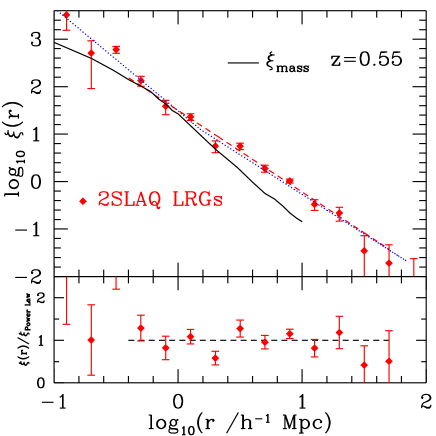
Figure 9: The real-space 2-point correlation function for the 2SLAQ LRG Survey (filled, red, diamonds) for the $\Lambda$ cosmology. The best-fit single power-law with $r_{0}=7.45\pm 0.35$ and $\gamma=1.72\pm{0.06}$ is given by the dashed (red) line. The double power-law fit reported for the angular correlation, $w(\theta)$, in Section 3.1, is shown by the dotted (blue) line. The solid (black) line is a theoretical prediction for the $\xi_{\rm mass}(z=0.55)$ using the simulations from Colín et al. (1999). These models have $(\Omega_{\rm m}$,$\Omega_{\Lambda})=$ $(0.3,0.7)$, $h=0.7$ and a $\sigma_{8}=1.0$. We shall return to this in Section 4. The lower panel shows the 2SLAQ LRG $\xi(r)$ measurements (assuming a $\Lambda$ cosmology) divided by this best-fitting power law with the dashed line covering $0.4<\sigma<50\;h^{-1}{\rm Mpc}$.

Table 5: Values of the correlation length and slope for the 2SLAQ LRG Survey from the real-space correlation function, $\xi(r)$. Model fits were performed over the range $0.4<r<50\;h^{-1}{\rm Mpc}$ for the $\Lambda$ cosmology and over the range $0.25<r<40\;h^{-1}{\rm Mpc}$ for the EdS cosmology.

	$\Lambda$	EdS
$r_{0}/\;h^{-1}{\rm Mpc}$	$7.45\pm 0.35$	$5.65\pm 0.41$
$\gamma$	$1.72\pm 0.06$	$1.67\pm 0.09$
$\chi^{2}_{min}$ (reduced)	1.73	0.62

Again, we attempt to fit simple power-law models to our $\xi(r)$ data in order to find values for the real-space correlation length and slope, $r_{0}$ and $\gamma$, respectively. For $\xi(r)$ we attempt to take into account the information presented in the covariance matrix by estimating $\chi^{2}$ fits to model $\xi(r)$ values such that

$$\chi^{2}=\sum_{i,j}[\bar{\xi}(r_{i})-\xi_{m}(r_{i})]\,C_{i,j}^{-1}\,[\bar{\xi}(r_{j})-\xi_{m}(r_{j})]$$ (20)

where $C_{ij}^{-1}$ is the inverse matrix of the covariance matrix and the subscripts $i$ and $j$ are indicies of separation bins. However, as has been reported in previous clustering analyses (e.g. Zehavi et al. (2002); Scranton et al. (2002)), the calculated covariance matrix is rather noisy with anti-correlations between points (contary to theoretical expectations). Therefore, when calculating the best-fitting models, we perform a simple $\chi^{2}$ fit as before, without the covariances, and take only the variances into account. As before, we fit over the scales $0.4\leq r\leq 50.0\;h^{-1}{\rm Mpc}$. For the case of the real-space correlation function, we again find that a single power-law may not fit the data well with the best-fit values (and related reduced $\chi^{2}$) given in Table 5. We find a value of $\gamma$ to be $1.72\pm 0.06$ and a correlation length of $r_{0}=7.45\pm 0.35$ (assuming a $\Lambda$ cosmology). The errors on these parameters are estimated from considering the 1$\sigma$ deivation from the minimized $\chi^{2}$ on the 1-parameter fits. However, care has to be taken when quoting the best fit values for the joint 2-parameter fits which are shown in Figure 10. Here we find the values of $\delta\chi^{2}$ which correspond to the 1, 2 and 3$\sigma$ levels for a 2-parameter fit. Also shown in Fig. 10 are the values for the deviations in $r_{0}$ and $\gamma$, if we find the 32 best-fitting single power-law parameters from the jackknife samples. Jackknife appears to confirm the $\chi^{2}$ error analysis with the assumption of Gaussian errors in Fig. 10. This is somewhat surprising since we have ignored the covariance between correlation function points in creating Fig. 10. The explanation may be that the fit at the minimum is still poor due to the deviant point at $2\;h^{-1}{\rm Mpc}$ in Fig. 9 and this causes the error contours in Fig. 10 to be larger than they would be in the absence of the deviant point. Including the full covariance matrix, the $\Delta\chi^{2}$ produces error contours significantly smaller than those in Fig. 10 and also the jackknife errors, even though the $\chi^{2}$ at minimum remained the same. Overall we take the errors in Fig. 10 supported by the jackknife estimates as being reasonably representative of the real error.

Figure 10: The joint 2 parameter fits on $r_{0}$ and $\gamma$ for $\xi(r)$. The contours show the $\delta\chi^{2}=(2.3,6.17,11.8)$ corresponding to 1, 2 and 3$\sigma$. The crosses show the deviations in $r_{0}$ and $\gamma$ that we find from the 32 best-fitting single power-law using the jackknife samples.

Now armed with our best-fitting single power-law model for $\xi(r)$, and we can proceed and see if modelling the redshift-space distortions introduced into the clustering pattern reveals anything about cosmological parameters.

4 LRG clustering and Cosmological Implications

Having calculated the $z$-space, projected and real-space correlation functions for the 2SLAQ Luminous Red Galaxies, we can now turn our attention to using these results to see if we can determine cosmological parameters.

4.1 The $\xi(\sigma,\pi)$ LRG Measurements

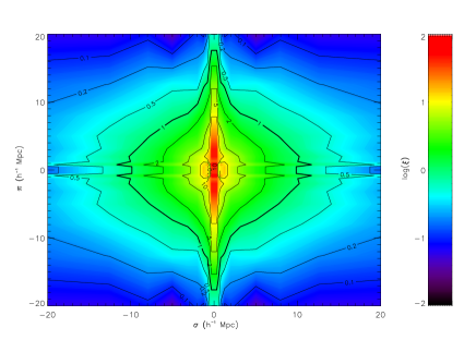
Figure 11: The $\xi(\sigma,\pi)$ contour plot for the 2SLAQ LRG Survey, assuming a $\Lambda$ cosmology of $(\Omega_{\rm m},\Omega_{\Lambda})=(0.3,0.7)$. The “Finger-of-God” effects, i.e. elongation of contours in the $\pi$ direction at small ($\lower 3.22916pt\hbox{$\sim$}\hbox to0.0pt{\hss\raise 1.1625pt\hbox{$<$}}1\;h^{-1}{\rm Mpc}$) scales, are clearly seen. (The spikes at small $\pi$ are a plotting artefacts).

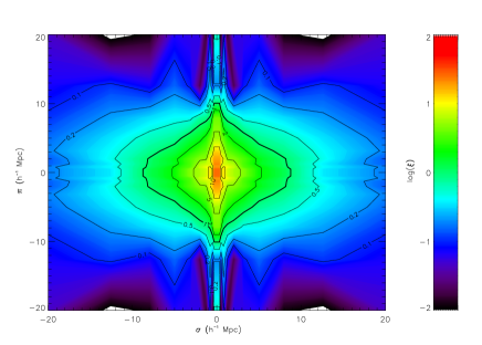
Figure 12: The $\xi(\sigma,\pi)$ contour plot for the 2SLAQ LRG Survey, with a $\Omega_{\rm m}=1.0$, EdS cosmology.

Results for the 2-D clustering of 2SLAQ LRGs are shown in the $\xi(\sigma,\pi)$ plots of Figures 11 and 12.

Galaxy peculiar velocities lead to distortions in the $\xi(\sigma,\pi)$ shape. The predominant effect at large scales in $\sigma$ is the coherent infall that causes a flattening of the $\xi(\sigma,\pi)$ contours along the parallel $\pi$ direction and some elongation along the perpendicular $\sigma$ direction. At small $\sigma$, the random peculiar motions of the galaxies cause an elongation of the clustering signal along the $\pi$ direction - the so-called “Fingers-of-God” effect. From the measurements of these effects, determination of the coherent infall into clusters, given by the parameter $\beta$, and the pairwise velocity dispersion, $\langle w_{\rm z}^{2}\rangle^{1/2}$, can be made. This calculation shall be performed in Section 4.2. Geometric distortions also occur if the cosmology assumed to convert the observed galaxy redshifts is not the same as the true, underlying cosmology of the Universe. The reason for this is because the cosmology dependence of the separations along the redshift direction is not the same as for the separations measured in the perpendicular direction (Alcock & Paczynski, 1979). We note that modelling the geometric distortions and comparing to the presented data can yield information on cosmological parameters.

We shall closely follow the methods of Hoyle et al. (2002) and da Ângela (2005), hereafter H02 and dA05, respectively. In this section, we first discuss large-scale, linear and small-scale non-linear $z$-space distortions and how they are parameterised by $\beta$ and $\langle w_{\rm z}^{2}\rangle^{1/2}$ respectively. We then use $\beta$ to find the bias of LRGs at the survey redshift. Next, we employ information gained in studying the geometric distortions to perform the “Alcock-Paczynski Test” as one route to calculating cosmological parameters. However, we realise there is a degeneracy in the $(\beta,\Omega_{\rm m})$ plane with this approach and thus employ further constraints from the evolution of LRG clustering to break this degeneracy.

4.2 Redshift-space distortions, $\beta$ and pairwise velocities

When measuring a galaxy redshift, one is actually measuring a sum of velocites. The total velocity comes from the Hubble expansion plus the motion induced by the galaxy’s local potential, where this second term is coined the “peculiar velocity”, i.e.

$$v_{\rm Tot}=v_{H}+v_{\rm pec}$$ (21)

The peculiar velocity itself contains two terms,

$$v_{\rm pec}=v_{\rm rand}+v_{\rm CI}$$ (22)

The first term, $v_{\rm rand}$ is due to the small-scale random motion of galaxies within clusters. The second term, $v_{\rm CI}$ is the component due to coherent infall around clusters, where the infall is caused by the streaming of matter from underdense to overdense regions; this leads to a “flattening” in the perpendicular $\sigma$-direction away from equi-distant contours in $\xi(\sigma,\pi)$. This extension is parameterised by $\beta$, which takes into account the large-scale effects of linear $z$-space distortions. Kaiser (1987) showed that, assuming a pure power-law model for the real-space correlation function (which is fair for the 2SLAQ LRG data), one can estimate $\beta$ in the linear regime using

$$\xi(s)=\xi(r)\left({1+\frac{2}{3}\beta+\frac{1}{5}\beta^{2}}\right).$$ (23)

and more generally

$$\xi(\sigma,\pi)=\left[1+\frac{2(1-\gamma\mu^{2})}{3-\gamma}\beta\\ +\frac{3-6\gamma\mu^{2}+\gamma(2+\gamma)\mu^{4}}{(3-\gamma)(5-\gamma)}\beta^{2}\right]\xi(r),$$ (24)

where $\mu$ is the cosine of the angle between $r$ and $\pi$ (the distance along the line of sight), and $\gamma$ is slope of the power law (Matsubara & Suto, 1996).

Even though the “Kaiser Limit” is a widely used method for estimating $\beta$, drawbacks using this approach, under the assumption of Gaussianity, have been known for some time (Hatton & Cole, 1998). Scoccimarro (2004) has recently reported on the limitations of assuming a Gaussian distribution in the pairwise velocity dispersion $\sigma_{12}$, even at very large scales. Scoccimarro’s argument is that even at large scales, linear theory cannot be applied since one still has the effect of galactic motions induced on sub-halo scales i.e. galaxies that are separated by very large distances are still “humming” about inside their own dark mattter haloes. Thus for the remainder of the paper, we make a note of the new formalism in Scoccimarro (2004), but continue to use the Kaiser Limit, acknowledging its short-comings. We justify this by noting that we need better control on our ‘1st order’ statistical and systematic errors before applying the ‘2nd order’ Scoccimarro corrections. Future analysis may use the 2SLAQ LRG and QSO sample to make comparisons for small and large scale effects in the redshift distortions using both the new Scoccimarro expression as well as the Kaiser Limit.

The small-scale random motions of the galaxies, $v_{\rm rand}$, leads to an extension in the $\pi$-direction of $\xi(\sigma,\pi)$. We denote the magnitude of this extension by $\langle w_{\rm z}^{2}\rangle^{1/2}$ ($\equiv\sigma_{12}$); this is usually expressed in a Gaussian form (e.g. dA05)

$$f(w_{z})=\frac{1}{\sqrt{2\pi}\langle w_{z}^{2}\rangle^{1/2}}\rm{exp}\left(-\frac{1}{2}\frac{|w_{z}|}{\langle w_{z}^{2}\rangle^{1/2}}\right).$$ (25)

Now we can combine these small-scale non-linear $z$-space distortions with the Kaiser formulae, and hence the full model for $\xi(\sigma,\pi)$ is given by

$$\xi(\sigma,\pi)=\int^{\infty}_{-\infty}\xi^{\prime}[\sigma,\pi-w_{z}(1+z)/H(z)]f(w_{z})dw_{z}$$ (26)

where $\xi^{\prime}[\sigma,\pi-w_{z}(1+z)/H(z)]$ is given by equation 24 and $f(w_{z})$ by equation 25. Using these expressions and our 2SLAQ LRG data, we can calculate $\beta$ and $\langle w_{\rm z}^{2}\rangle^{1/2}$ for the LRGs. At this juncture, it is important to note the scales we consider in our model. As can be seen from the data presented in Section 3, a power-law fits the data best on scales from 1 to 20 $\;h^{-1}{\rm Mpc}$. Thus, when computing the full model for $\xi(\sigma,\pi)$ (equation 26), we only use data with $1<\sigma<20\;h^{-1}{\rm Mpc}$ and $1<\pi<20\;h^{-1}{\rm Mpc}$ (as shown in Figures 11 and 12).

Returning to Kaiser (1987), the value of $\beta$ can be used to determine the bias, $b$, of the objects in question,

$$\beta\simeq\frac{\,\Omega_{\rm m}^{\,0.6}}{b}$$ (27)

provided you know the values of $\Omega_{\rm m}$, where $\Omega_{\rm m}(z)$ is given by

$$\Omega_{\rm m}(z)=\frac{\Omega_{\rm m}^{0}(1+z)^{3}}{\Omega_{\rm m}^{0}(1+z)^{3}+\Omega_{\Lambda}^{0}},$$ (28)

for a flat universe. The importance of the bias is that it links the visible galaxies to the underlying (dark) matter density fluctuations,

$$\delta_{g}=b\;\;\delta_{m}$$ (29)

where the $g$ and the $m$ subscripts stand for galaxies and mass respectively. However, the precise way in which galaxies trace the underlying matter distribution is still poorly understood. Recent work by e.g. Blanton et al. (2006), Schulz & White (2006), Smith et al. (2007) and Coles & Erdogdu (2007) suggests that bias is potentially scale-dependent and we note that we do not take this into account in the current analysis. Thus, for our purposes, we restrict ourselves to the very simple relation, $\xi_{g}=b^{2}\xi_{m}$, where $b$ is the linear bias term and leave further investigation of the bias for massive galaxies at intermediate redshift to a future paper. On the above model assumptions we now proceed to estimate the cosmological parameters, $\Omega_{\rm m}$ and $\beta$.

4.3 Cosmological Parameters from $\xi(\sigma,\pi)$ models.

The ratio of observed angular size to radial size varies with cosmology. If we have an object which is known to be isotropic, i.e. where transverse and radial intrinsic size are the same, fixing the ratio of the intrinsic radial and transverse distances yields a relation between the measured radial and transverse distances depending on cosmological parameters. This comparison is often called the “Alcock-Paczynski” test (Alcock & Paczynski 1979; Ballinger, Peacock & Heavens 1996). In order to perform this test, we assume galaxy clustering is, on average, isotropic and we compare data and model cosmologies. Following H02 and dA05, for the following sections, we define several terms.

(i) The Underlying cosmology - this is the true, underlying, unknown cosmology of the Universe.

(ii) The Assumed cosmology - the cosmology used when measuring the two-point correlation function and $\xi(\sigma,\pi)$ from the 2SLAQ LRG survey. Initially in a redshift survey, the only information available is the object’s position on the sky and its redshift. In order to convert this into a physical separation, you must assume some cosmology. As was mentioned earlier, we have considered two Assumed cosmologies, the $\Lambda$ $(\Omega_{\rm m}$, $\Omega_{\Lambda})$ = (0.3,0.7) and the EdS $(\Omega_{\rm m},\Omega_{\Lambda})$ = (1.0,0.0) cases.

(iii) The Test Cosmology - the cosmology used to generate the model predictions for $\xi(\sigma,\pi)$ which are then translated into the assumed cosmology.

We compare the geometric distortions in both the data and the model relative to the same Assumed cosmology. Thus, the key to this technique lies in the fact that when the Test cosmology matches the Underlying cosmology, the distortions introduced into the clustering pattern should be the same in model as in the data. The model should then provide a good fit to the data, providing the redshift-space distortions have been properly accounted for. We can then endeavour to find values of $\Omega_{\rm m}$ and $\beta$. We assume that for all further discussions, the cosmologies described are spatially flat and choose to fit the variable $\Omega_{\rm m}^{0}$, hence fixing $\Omega_{\Lambda}^{0}=1-\Omega_{\rm m}^{0}$.

The relation between the separations $\sigma$ and $\pi$ in the Test and Assumed cosmologies (referred to by the subscripts $t$ and $a$ respectively) is the following (Ballinger et al. 1996, HO2, dA05):

$$\sigma_{t}=f_{\perp}\sigma_{a}=\frac{B_{t}}{B_{a}}\sigma_{a}$$ (30)

$$\pi_{t}=f_{\parallel}\pi_{a}=\frac{A_{t}}{A_{a}}\pi_{a}$$ (31)

where $A$ and $B$ are defined as follows (for spatially flat cosmologies):

$$A=\frac{c}{H_{0}}\frac{1}{\sqrt{\Omega_{\Lambda}^{0}+\Omega_{\rm m}^{0}(1+z)^{3}}}$$ (32)

$$B=\frac{c}{H_{0}}\int_{0}^{z}\frac{dz^{\prime}}{\sqrt{\Omega_{\Lambda}^{0}+\Omega_{\rm m}^{0}(1+z^{\prime})^{3}}}.$$ (33)

In the linear regime, the correlation function in the assumed cosmology will be the same as the correlation function in the test cosmology, given that the separations are scaled appropriately. i.e.:

$$\xi_{t}(\sigma_{t},\pi_{t})=\xi_{a}(\sigma_{a},\pi_{a}).$$ (34)

Details on the fitting procedure are given in dA05 (Section 7.7). Using this AP-distortion test, we calculate values of $\Omega_{\rm m}$-$\beta$ for the assumed $\Lambda$ cosmology. and present them in Figure 13. We first note that the constraint here is almost entirely on $\beta$ rather than $\Omega_{\rm m}$. Using the $\xi(r)$ fit with a (starting) $r_{0}=7.45\;h^{-1}{\rm Mpc}$ and $\gamma=1.72$, we find that $\Omega_{\rm m}=0.10^{+0.35}_{-0.10}$ and $\beta(z=0.55)=0.40\pm 0.05$ with a velocity dispersion of $\sigma=330$kms^-1 from a $\chi^{2}$ minimization. We have checked these errors by repeating the above calculations on the 32 “jackknife” sub-samples. In order to make the jackknife calculations less computationally intensive, the velocity dispersion is held fixed at 330${\rm~{}km~{}s}^{-1}$ in every case. Comparing the error contours in Fig. 13 with the jackknife estimates, we again find that the jackknife errors for $\beta$ at $\pm 0.05$ are comparable to, if not smaller than, those in the error contours in Fig. 13. The jackknife error in $\Omega_{\rm m}$ at $\pm 0.14$ is comparable to the error contour in Fig. 13. As in Fig. 10, this agreement may be surprising given that we have ignored the covariance in $\xi(\sigma,\pi)$ points which is almost certainly non-negligible. Again we argue that a relatively poor $\chi^{2}$ fit at minimum may be responsible, leading to a somewhat fortuitous agreement of the formal and jackknife error. But on the grounds of the jackknife results we believe that the error contours shown in Fig. 13 are reasonably realistic and we shall quote these hearafter.

We have also fitted $\xi(\sigma,\pi)$ assuming an EdS cosmology. In principle this should give the same result as assuming the $\Lambda$ model. We show these $\Omega_{\rm m}-\beta$ fits in Figure 14. We find that the best fit is now $\Omega_{\rm m}=0.40^{+0.6}_{-0.25}$ and $\beta=0.45^{+0.20}_{-0.10}$ ($\chi^{2}$ minimization) with a velocity dispersion of $\sigma=330$kms^-1. A model with $\gamma=1.67$ and a (starting) correlation length of $r_{0}=5.65\;h^{-1}{\rm Mpc}$ is used. Thus the $\beta$ and the velocity dispersion values are reasonably consistent with the previous result. However, the value of $\Omega_{\rm m}$ assuming an EdS cosmology, is somewhat higher than the best-fit found assuming a $\Lambda$ cosmology. We assume that the high degeneracy of $\Omega_{\rm m}$ coupled with slightly different $\xi(r)$ models in the two cases is causing this discrepancy. The contours in Fig. 14 certainly suggest that the constraint on $\Omega_{\rm m}$ is much less strict in the EdS assumed case.

We have investigated other systematics in the $\Omega_{\rm m}-\beta$ fits. Returning to an assumed $\Lambda$ cosmology, there is some small dependence on the model assumed for $\xi(r)$. For example, if the slope $\gamma=1.69$ from fitting $\xi(r)$ in the more limited range $0.4<r<20$h^-1Mpc is assumed then we find that $\Omega_{\rm m}=0.10\pm 0.29$ and $\beta(z=0.55)=0.35\pm 0.16$ with a velocity dispersion of $\sigma=300$kms^-1. Further, if instead of using $\xi(r)$, $w_{p}(\sigma)$ is used with slope $\gamma=1.83$ over the usual $0.4<r<50\;h^{-1}{\rm Mpc}$ range, we find that the best-fit model prefers a very low value of $\Omega_{\rm m}=0.02\pm 0.15$ and $\beta(z=0.55)=0.40\pm 0.05$ with a velocity dispersion of $\sigma=360$kms^-1. The consistency of these different models to give values of $\Omega_{\rm m},\beta$ and a pairwise velocity dispersion, albeit at a cost of a very loose constraint on $\Omega_{\rm m}$, is re-assuring and summarised in Table 6. Since $w(\theta)$ also seems to indicate a flatter ($\gamma=-1.67\pm{0.07}$) slope in the $1<r<20\;h^{-1}{\rm Mpc}$ range of interest for $\xi(\sigma,\pi)$ we take our ‘best bet’ estimates to be the values for $\gamma=-1.72$ given above. These values also give a good overall fit to $\xi(s)$. We next introduce a further constraint to break the $\Omega_{\rm m}-\beta$ degeneracy.

Table 6: Best fitting model values of $\Omega_{\rm m},\beta$ and pairwise velocity dispersion, $\langle w_{\rm z}^{2}\rangle^{1/2}$, using redshift-space distortions alone and assuming a $\Lambda$ cosmology.

$r_{0}$	$\gamma$	range /$\;h^{-1}{\rm Mpc}$	Measure	$\Omega_{\rm m}$	$\beta$	$\langle w_{\rm z}^{2}\rangle^{1/2}/{\rm~{}km~{}s}^{-1}$
7.45	1.72	0.4-50	$\xi(r)$	0.10	0.40	330
7.30	1.83	0.4-50	$w_{p}(\sigma)$	0.02	0.40	360
7.60	1.68	0.4-20	$\xi(r)$	0.10	0.35	300
7.34	1.80	0.4-20	$w_{p}(\sigma)$	0.10	0.45	360

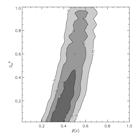
Figure 13: Likelihood contours of $\Omega_{\rm m}^{0}$-$\beta(z=0.55)$ using the geometric method of Alcock-Paczynski test and modelling the redshift-space distortions. The best-fit values are $\Omega_{\rm m}=0.10^{+0.35}_{-0.10}$ and $\beta(z=0.55)=0.40\pm 0.05$ with a velocity dispersion of $\sigma=330$kms^-1. Note how a value of $\Omega_{\rm m}\sim 0.3$ is not ruled out but also the large degeneracy along the $\Omega_{\rm m}$ direction. A $\Lambda$ cosmology is assumed, along with a model where $\gamma=1.72$ and a (starting) value of $r_{0}=7.45\;h^{-1}{\rm Mpc}$.

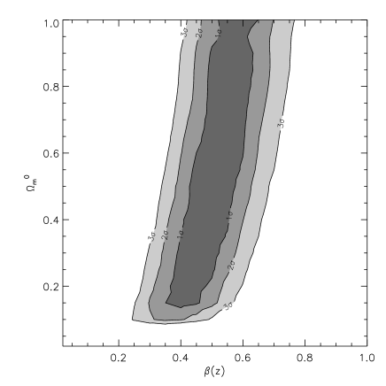
Figure 14: Likelihood contours of $\Omega_{\rm m}^{0}$-$\beta(z=0.55)$ using the geometric method of Alcock-Paczynski test and modelling the redshift-space distortions, assuming an EdS cosmology. The best-fit values are $\Omega_{\rm m}=0.40^{+0.60}_{-0.25}$ and $\beta=0.45^{+0.20}_{-0.10}$ using a model with $\gamma=1.67$ and a (starting) correlation length of $r_{0}=5.65\;h^{-1}{\rm Mpc}$. A value of $\Omega_{\rm m}\sim 1.0$ lies within our 1$\sigma$ contour but again there is a large degeneracy along the $\Omega_{\rm m}$ direction.

4.4 Further Constraints on $\Omega_{0}^{\rm m}$ and $\beta(z)$ from LRG Clustering Evolution

Matsubara & Suto (1996) and Croom & Shanks (1996) pointed out that by combining low redshift and high redshift clustering information, further constraints on $\Omega_{\rm m}$ and $\Omega_{\Lambda}$ would be possible. The basic idea described in this section is that the $\Omega_{\rm m}$:$\beta(z)$ degenerate set obtained from LRG clustering evolution is different from the $\Omega_{\rm m}$:$\beta(z)$ degenerate set obtained from analysing LRG redshift-space distortions; by using these two constraints in combination, the degeneracies may be lifted. Thus the way we proceed to break the degeneracy is to combine our current 2SLAQ LRG results with constraints derived from consideration of LRG clustering evolution.

From the value of the mass correlation function at $z=0$, linear perturbation theory can be used, assuming a test $\Omega_{\rm m}$, to compute the value of the mass correlation function in real space at $z=0.55$. This can then be compared to the measured LRG $\xi(r)$ at $z=0.55$ to find the value of the bias $b(z=0.55)$. The clustering of the mass at $z=0$ can be determined if the galaxy correlation function is known, assuming that the bias of the galaxies used, $b(z=0)$, is independent of scale. Fortunately, recent galaxy redshift surveys have obtained precise measurements of the clustering of galaxies at $z\approx 0$. In practice we shall start from $\xi(s)$ at $z=0$ and $z=0.55$ and use equation 23 to derive $\xi(r)$ in each case.

We therefore follow da Ângela et al. (2005) and start by introducing the volume averaged two-point correlation function $\bar{\xi}$ where

$$\bar{\xi}(s)=\frac{\int_{0}^{s}4\pi s^{\prime 2}\xi(s^{\prime})ds}{\int_{0}^{s}4\pi s^{\prime 2}ds}$$ (35)

We do this so that non-linear effects in the sample should be insignificant due to the $s^{2}$ weighting, setting the upper limit of the integral $s=20\;h^{-1}{\rm Mpc}$. To calculate equation 35 at $z=0$, we use the double-power law form that is found by the 2dFGRS to describe $\xi(s)$ (Hawkins et al., 2003, Fig. 6) in the numerator.

Then, the equivalent averaged correlation function in real-space can be determined by

$$\bar{\xi}(r,z=0)=\frac{\bar{\xi}(s,z=0)}{1+\frac{2}{3}\beta(z=0)+\frac{1}{5}\beta(z=0)^{2}}$$ (36)

where $\bar{\xi}(s)$ comes from equation 35 and we take the value of $\beta$ for the 2dFGRS as $\beta(z=0)=0.49\pm 0.09$ (Hawkins et al., 2003). Now the real-space mass correlation is obtained with

$$\bar{\xi}_{\rm mass}(r,z=0)=\frac{\bar{\xi}(r,z=0)}{b(z=0)^{2}},$$ (37)

where $b(z=0)$ is given for each test cosmology by

$$b(z=0)=\frac{\Omega^{0.6}_{\rm m}(z=0)}{\beta(z=0)}.$$ (38)

Once we have determined the real-space correlation function of the mass at $z=0$, its value at $z=0.55$ is obtained using linear perturbation theory. Hence, at $z=0.55$, the real-space correlation function of the mass will be:

$$\bar{\xi}_{\rm mass}(r,z=0.55)=\frac{\bar{\xi}_{\rm mass}(r,z=0)}{G(z=0.55)^{2}},$$ (39)

Here, $\bar{\xi}_{\rm mass}(r)$ is the volume-averaged correlation function (with $1\leq r\leq 20\;h^{-1}{\rm Mpc}$) and $G(z)$ is the growth factor of perturbations, given by linear theory (Carroll et al., 1992; Peebles, 1980) and depends on cosmology - in this case the test cosmology.

Once the value of $\bar{\xi}_{\rm mass}(r,z=0.55)$ is obtained for a given test cosmology, the process to find $\beta(z=0.55)$ is similar to the one used to find $\bar{\xi}_{\rm mass}(r,z=0)$, but now the steps are performed in reverse: $\bar{\xi}(s,z=0.55)$ can be measured in a similar way as $\bar{\xi}(s,z=0)$. The bias factor at $z\approx 0.55$ is given by:

$$b^{2}(z=0.55)=\frac{\bar{\xi}(r,z=0.55)}{\bar{\xi}_{\rm mass}(r,z=0.55)},$$ (40)

where $\bar{\xi}_{\rm mass}(r)$ is given by equation 39 and $\bar{\xi}(r,z=0.55)$ is obtained by:

$$\bar{\xi}(r,z=0.55)=\frac{\bar{\xi}(s,z=0.55)}{1+\frac{2}{3}\beta(z=0.55)+\frac{1}{5}\beta(z=0.55)^{2}}.$$ (41)

The value of $\beta(z=0.55)=\Omega_{\rm m}^{0.6}(z=0.55)/b(z=0.55)$ will be obtained, for the given test value of $\Omega_{\rm m}(z=0)$ by solving the second order polynomial formed by substituting $\bar{\xi}(r,z=0.55)$ from equation 40 into equation 41 (see Hoyle et al., 2002). The confidence levels on the computed values of $\beta(z=0.55)$ are calculated by combining appropriately in quadrature the errors on $\bar{\xi}(s,z=0.55)$, $\bar{\xi}(s,z=0)$, $\beta(z=0.55)$ and $\beta(z=0)$.

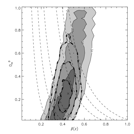
Figure 15: Joint likelihood contours of $\Omega_{\rm m}^{0}$-$\beta(z=0.55)$ using the geometric method of Alcock-Paczynski test, modelling the redshift-space distortions and including the evolution of clustering constraints, assuming the $\Lambda$ cosmology. Here we see that the best-fit joint constraint values are $\Omega_{\rm m}=0.25^{+0.10}_{-0.15}$, $\beta=0.45\pm 0.05$ (marked with the cross) with a $\langle w_{\rm z}^{2}\rangle^{1/2}$ of $330\rm kms^{-1}$.

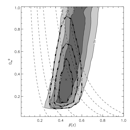
Figure 16: Joint likelihood contours for $\Omega_{\rm m}^{0}$-$\beta(z=0.55)$ using the geometric method of Alcock-Paczynski test, modelling the redshift-space distortions and including the evolution of clustering constraints, assuming an EdS cosmology. The joint best-fit has $\Omega_{\rm m}=0.35\pm 0.15$, $\beta=0.45\pm 0.05$ (marked with the cross) and a $\langle w_{\rm z}^{2}\rangle^{1/2}$ of $330\rm kms^{-1}$. When the joint constraints are considered, a value of $\Omega_{\rm m}=1.0$ can be ruled out at the 3$\sigma$ level.

Combining this clustering evolution constraint with those from $z$-space distortions breaks the degeneracy in the $\Omega_{\rm m}-\beta$ plane. We can now work out the joint-2 parameter best fitting regions. This is shown in Figure 15, where the 1, 2 and 3 sigma error bars are plotted (dashed lines). The best fitting 2-parameter calculations has $\Omega_{\rm m}=0.25$, $\beta=0.45$ denoted by the cross in Figure 15. When we consider the 1-sigma error on each quantity separately we find, $\Omega_{\rm m}=0.25^{+0.10}_{-0.15}$, $\beta=0.45\pm 0.05$ with a $\langle w_{\rm z}^{2}\rangle^{1/2}$ of $330\rm kms^{-1}$. A model $\xi(r)$ is assumed with $\gamma=1.72$ and $r_{0}=7.45\;h^{-1}{\rm Mpc}$, as is a $\Lambda$ cosmology.

The case of the combined constraint for the EdS assumed cosmology is shown in Figure 16. The $\xi(r)$ model with $\gamma=1.67$ and $r_{0}=5.65\;h^{-1}{\rm Mpc}$ is assumed and we find $\Omega_{\rm m}=0.35\pm 0.15$ and $\beta=0.45\pm 0.05$. Although the 3-sigma contours still reject the EdS model, the rejection is less than in the $\Lambda$ assumed case. Overall we conclude that the combined constraints on $\beta$ are the strongest with $\beta=0.45\pm 0.05$ consistently produced whatever the assumed cosmology or $\xi(r)$ model. Though the combined constraints on $\Omega_{\rm m}$ are less strong and give $\Omega_{\rm m}\approx 0.3\pm 0.15$, they still appear consistent with the standard $\Lambda$ model.

As another check, we can use the ratio $\xi(s)/\xi(r)$ to determine $\beta$ from equation 23 (see Figure 17). We assume that $\beta$ is scale-independent, the $z$-space distortions are only affected by the large-scale infall and are not contaminated by random peculiar motions. Fitting over the scales, $5<s<50\;h^{-1}{\rm Mpc}$, we find $\beta=0.47\pm 0.14$, which is consistent with our determination using the distortions. The 1-$\sigma$ error comes from a standard $\chi^{2}$ analysis using the $\xi(s)/\xi(r)$ ratios and their errors; these are derived from adding the jackknife errors on $\xi(s)$ and $\xi(r)$ in quadrature. We note that this procedure does not take into account the non-independence of the correlation function points, suggesting that the relatively large error quoted above on $\beta$ may still be a lower limit.

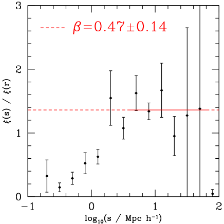
Figure 17: The ratio of the redshift-space correlation function to the real-space correlation function, measured from the 2SLAQ LRG survey. We assume a $\Lambda$ cosmology for these measurements and fitting over the scales of 5 - 50 $\;h^{-1}{\rm Mpc}$ find that $\beta=0.47\pm 0.14$, in very good agreement with our redshift-space distortion/evolution of clustering technique measurements.

The low values of $\Omega_{\rm m}\approx 0.30$ and the value of $\beta=0.45$ we find from the 2SLAQ LRG survey are in line with what is generally expected in the current standard cosmological model. Although the constraint on $\beta$ is tight, the constraint on $\Omega_{\rm m}$ is less so and in particular the EdS value is not rejected at 3$\sigma$ when clustering distortions only are considered. However, when the combined evolution and redshift distortions are considered, the EdS value is rejected at the 3$\sigma$ level.

Using equations 40, 41, $\Omega_{\rm m}(z=0)=0.30\pm 0.15$ and $\beta(z=0.55)=0.45\pm 0.05$, we find that $b(z=0.55)=\Omega^{0.6}_{\rm m}(z=0.55)/\beta(z=0.55)=1.66\pm 0.35$, showing that the 2SLAQ LRGs are highly biased objects. This can be compared with the value for SDSS LRGs at redshift $z=0.55$ which are found to have a value of $b=1.81\pm 0.04$ (Padmanabhan et al. 2006, Fig. 13). The 2SLAQ LRG value is consistent with this SDSS LRG value; of course a slightly lower bias may have been expected for 2SLAQ LRGs due to the bluer/lower luminosity selection cut. If we assume the value found in recent studies of $\Omega_{\rm m}(z=0)=0.25$ (Cole et al., 2005; Eisenstein et al., 2005; Tegmark et al., 2006; Percival et al., 2006a, b), then our esimate of $b$ becomes $b=1.56\pm 0.33$.

Although we leave discussion about the bias estimate and the accuracy of the $\beta$-model to a future paper, at the referee’s request, we compare the non-linear mass correlation function as numerically calculated for the standard cosmology (Colín et al., 1999) to the 2SLAQ LRG $\xi(r)$, in Figure 9. The errors in $\xi(\sigma,\pi)$ are smaller at separations 5 to 20 $\;h^{-1}{\rm Mpc}$, than at $1\;h^{-1}{\rm Mpc}$, so our estimates of bias from $\xi(\sigma,\pi)$ are weighted towards these larger scales where there appears to be approximate consistency with the relative amplitudes of $\xi_{\rm mass}$ and $\xi(r)$ in Fig. 9. Thus, as mentioned previously, our working assumption from here on will be that there is no effect of scale-dependent bias on our $\Omega_{\rm m}-\beta$ fits and we leave further investigation of this issue for future work.

Finally, taking the value of $b(z=0.55)=1.66\pm 0.35$, we can relate $b(z=0)$ to $b(0.55)$ using the bias evolution model (Fry, 1996)

$$b(z)=1+[b(0)-1]G(\Omega_{\rm m}(0),\Omega_{\Lambda}(0),z),$$ (42)

where $G(\Omega_{\rm m}(0),\Omega_{\Lambda}(0),z)$ is the linear growth rate of the density perturbations (Peebles, 1980, 1984; Carroll et al., 1992). There are many other bias models, but here we are making the simple assumptions that galaxies formed at early times and their subsequent clustering is governed purely by their discrete motion within the gravitational potential produced by the matter density perturbations. This model would be appropriate, for example, in a “high-peaks” biasing scenario where early-type galaxies formed at a single redshift and their co-moving space density then remained constant to the present day. There may be evidence for such a simple evolutionary history in the observed early-type stellar mass/luminosity functions (e.g. Metcalfe et al., 2001; Brown et al., 2006; Wake et al., 2006). From equation 42, and taking $b(0.55)=1.66$, implies a value today of $b(0)=1.52$ at $z\sim 0.1$. This leads to a predicted correlation length today of $r_{0}(z=0)=8.5\pm 1.6\;h^{-1}{\rm Mpc}$ (assuming $\Lambda$CDM) which is consistent with the 2dFGRS value of $r_{0}=8.0\pm 1.0\;h^{-1}{\rm Mpc}$ found from averaging the same two matched luminosity bins from Table 2 of Norberg et al. (2002), and previously used in our Fig. 7. (But note that the 2dFGRS $\xi(s)$ shown in Fig. 7 might imply a somewhat lower value for the 2dFGRS clustering amplitude in this bin than $r_{0}=8.0\pm 1.0\;h^{-1}{\rm Mpc}$.)

Therefore, these correlation function evolution results suggest that there seems to be no inconsistency with the idea that the LRGs have a constant co-moving space density, as may be suggested by the luminosity function results. But, we note that the LF results of Wake et al. (2006) apply to a colour-cut sample, (where 2SLAQ LRGs are carefully matched to SDSS LRGs) whereas our clustering results are only approximately matched to the 2dFGRS. It will be interesting to see if this results holds when the clustering of the exactly matched high and low redshift LRGs are compared (see Wake et al., 2007, in prep.).

5 conclusions

We have performed a detailed analysis of the clustering of 2SLAQ LRGs in redshift space as described by the two-point correlation function. Our main conclusions are as follows.

1. The LRG two-point correlation function, $\xi(s)$, averaged over the redshift range $0.4<z<0.8$, shows a slope which changes as a function of scale, being flatter on small scales and steeper on large scales, consistent with the expected effects of redshift-space distortions.

2. The best fitting single power-law model to the Real-space 2-Point correlation function of the 2SLAQ LRG Survey has a clustering length of $r_{0}=7.45\pm 0.35\;h^{-1}{\rm Mpc}$ and a power-law slope of $\gamma=1.72\pm 0.06$ (assuming a $\Lambda$ cosmology) showing LRGs to be highly clustered objects.

3. Evidence for a change in the slope of the projected correlation function, which is a prediction of halo occupation distribution (HOD) models, is seen in the 2SLAQ LRG survey results, while a stronger feature is observed in the angular correlation function of the LRGs. A direct explanation for this remains unclear.

4. From redshift distortion models and the geometric Alcock-Paczynski test we find $\Omega_{\rm m}=0.10^{+0.35}_{-0.10}$ and $\beta(z=0.55)=0.40\pm 0.05$ with a velocity dispersion of $\sigma=330$kms^-1, assuming a $\Lambda$ cosmology. With EdS as the assumed cosmology, $\Omega_{\rm m}=0.40^{+0.60}_{-0.25}$ and $\beta=0.45^{+0.20}_{-0.10}$ with the best-fitting velocity dispersion remaining at $\sigma=330$kms^-1. However, in both cases, we also find a degeneracy along the $\Omega_{\rm mass,0}$-$\beta$ plane.

5. By considering the evolution of clustering from $z\sim 0$ to $z_{\rm LRG}=0.55$ we can break this degeneracy and find that $\Omega_{\rm m}=0.25^{+0.10}_{-0.15}$ and $\beta=0.45\pm 0.05$ (with a $\langle w_{\rm z}^{2}\rangle^{1/2}$ of $330\rm kms^{-1}$) assuming a $\Lambda$ cosmology. When the EdS cosmology is assumed, we find $\Omega_{\rm m}=0.35\pm 0.15$ and $\beta=0.45\pm 0.05$ (again $\langle w_{\rm z}^{2}\rangle^{1/2}=330\rm kms^{-1}$). When the joint constraints are considered, a value of $\Omega_{\rm m}=1.0$ can be ruled out at the 3$\sigma$ level. We believe these estimates of $\beta(z=0.55)$ are reasonably robust but the values of $\Omega_{\rm m}$ are less well constrained, although the above estimate for $\Omega_{\rm m}=0.30\pm{0.15}$ is in agreement with concordance values.

6. If we assume a $\Lambda$ cosmology with $\Omega_{\rm m}(z=0)=0.3$ and $\beta(z=0.55)=0.45$ then the value for the 2SLAQ LRG bias at $\bar{z}=0.55$ is $b=1.66\pm 0.35$, in line with other recent measurements of LRG bias (Padmanabhan et al. 2006).

7. Assuming this $b(z=0.55)=1.66$ value, and adopting a simple “high-peaks” bias prescription which assumes LRGs have a constant co-moving space density, we predict $r_{0}=8.5\pm 1.6\;h^{-1}{\rm Mpc}$ for LRGs at $z\approx 0.1$. This is not inconsistent with the observed result for luminosity matched 2dFGRS ‘LRGs’ at this redshift.

The clustering and redshift-space distortion results complement the other results from the 2SLAQ Survey e.g. Wake et al. (2006), Wake et al. (2007, in prep.) and da Angela et al. (2006, in prep). Luminous Red Galaxies may be considered to be “red and dead” but they have recently been realised to be very powerful tools for both constraining galaxy formation and evolution theories as well as cosmological probes. Future projects utilising LRGs (e.g. to measure the baryon acoustic oscillations or to study LRGs at higher redshift/fainter magnitudes) will give us more insights into today’s greatest astrophysical problems, including the epoch of massive galaxy formation and the acceleration of the cosmological expansion.

References

- Alcock & Paczynski (1979) Alcock C., Paczynski B., 1979, Nature, 281, 358
- Ballinger et al. (1996) Ballinger W. E., Peacock J. A., Heavens A. F., 1996, MNRAS, 282, 877
- Blanton et al. (2006) Blanton M. R., Eisenstein D., Hogg D. W., Zehavi I., 2006, ApJ, 645, 977
- Brown et al. (2006) Brown M. J. I., Dey A., Jannuzi B. T., Brand K., Benson A. J., Brodwin M., Croton D. J., Eisenhardt P. R., 2006, pre-print (astro-ph/0609584)
- Cannon et al. (2006) Cannon R., et al., 2006, MNRAS, 372, 425
- Carroll et al. (1992) Carroll S. M., Press W. H., Turner E. L., 1992, ARAA, 30, 499
- Coil et al. (2004) Coil A. L., et al., 2004, ApJ, 609, 525
- Cole et al. (2005) Cole S., et al., 2005, MNRAS, 362, 505
- Coles & Erdogdu (2007) Coles P., Erdogdu P., 2007, astro-ph/0706.0412, 706
- Colín et al. (1999) Colín P., Klypin A. A., Kravtsov A. V., Khokhlov A. M., 1999, ApJ, 523, 32
- Croom et al. (2005) Croom S. M., et al., 2005, MNRAS, 356, 415
- Croom & Shanks (1996) Croom S. M., Shanks T., 1996, MNRAS, 281, 893
- Croom et al. (2004) Croom S. M., Smith R. J., Boyle B. J., Shanks T., Miller L., Outram P. J., Loaring N. S., 2004, MNRAS, 349, 1397
- da Angela et al. (2006) da Angela J., et al., 2006, astro-ph/0612401
- da Ângela et al. (2005) da Ângela J., Outram P. J., Shanks T., Boyle B. J., Croom S. M., Loaring N. S., Miller L., Smith R. J., 2005, MNRAS, 360, 1040
- Davis & Peebles (1983) Davis M., Peebles P. J. E., 1983, ApJ, 267, 465
- Eisenstein et al. (2001) Eisenstein D. J., et al., 2001, AJ, 122, 2267
- Eisenstein et al. (2005) Eisenstein D. J., et al., 2005, ApJ, 633, 560
- Fry (1996) Fry J. N., 1996, ApJL, 461, L65
- Fukugita et al. (1996) Fukugita M., Ichikawa T., Gunn J. E., Doi M., Shimasaku K., Schneider D. P., 1996, AJ, 111, 1748
- Hamilton (1993) Hamilton A. J. S., 1993, ApJ, 417, 19
- Hatton & Cole (1998) Hatton S., Cole S., 1998, MNRAS, 296, 10
- Hawkins et al. (2003) Hawkins E., et al., 2003, MNRAS, 346, 78
- Hoyle et al. (2002) Hoyle F., Outram P. J., Shanks T., Boyle B. J., Croom S. M., Smith R. J., 2002, MNRAS, 332, 311
- Jannuzi & Dey (1999) Jannuzi B. T., Dey A., 1999, in Weymann R., et al. eds, ASP Conf. Ser. 191: Photometric Redshifts and the Detection of High Redshift Galaxies p. 111
- Kaiser (1987) Kaiser N., 1987, MNRAS, 227, 1
- Landy & Szalay (1993) Landy S. D., Szalay A. S., 1993, ApJ, 412, 64
- Le Fèvre et al. (2005) Le Fèvre O., et al., 2005, A&AP, 439, 877
- Lewis et al. (2002) Lewis I. J., et al., 2002, MNRAS, 333, 279
- Li et al. (2006) Li C., Kauffmann G., Jing Y. P., White S. D. M., Börner G., Cheng F. Z., 2006, MNRAS, 368, 21
- Loveday et al. (1996) Loveday J., Peterson B. A., Maddox S. J., Efstathiou G., 1996, APJS, 107, 201
- Madgwick et al. (2003) Madgwick D. S., et al., 2003, MNRAS, 344, 847
- Martínez & Saar (2002) Martínez V. J., Saar E., 2002, Statistics of the Galaxy Distribution. Chapman & Hall/CRC
- Matsubara & Suto (1996) Matsubara T., Suto Y., 1996, ApJL, 470, L1+
- Matsubara & Szalay (2001) Matsubara T., Szalay A. S., 2001, ApJL, 556, L67
- Metcalfe et al. (2001) Metcalfe N., Shanks T., Campos A., McCracken H. J., Fong R., 2001, MNRAS, 323, 795
- Norberg et al. (2002) Norberg P., et al., 2002, MNRAS, 332, 827
- Peacock et al. (2001) Peacock J. A., et al., 2001, Nature, 410, 169
- Peebles (1980) Peebles P. J. E., 1980, The Large-Scale Structure of the Universe. Princeton University Press.
- Peebles (1984) Peebles P. J. E., 1984, ApJ, 284, 439
- Percival et al. (2002) Percival W. J., et al., 2002, MNRAS, 337, 1068
- Percival et al. (2006a) Percival W. J., et al., 2006a, astro-ph/0608635
- Percival et al. (2006b) Percival W. J., et al., 2006b, astro-ph/0608636
- Phillipps et al. (1978) Phillipps S., Fong R., Fall R. S. E. S. M., MacGillivray H. T., 1978, MNRAS, 182, 673
- Phleps et al. (2006) Phleps S., Peacock J. A., Meisenheimer K., Wolf C., 2006, A&AP, 457, 145
- Press et al. (1992) Press W. H., Teukolsky S. A., Vetterling W. T., Flannery B. P., 1992, Numerical Recipes in FORTRAN: The Art of Scientific Computing. Cambridge University Press.
- Ratcliffe et al. (1998) Ratcliffe A., Shanks T., Parker Q. A., Fong R., 1998, MNRAS, 296, 191
- Roseboom et al. (2006) Roseboom I. G., et al., 2006, pre-print, (astro-ph/0609178)
- Sánchez et al. (2006) Sánchez A. G., Baugh C. M., Percival W. J., Peacock J. A., Padilla N. D., Cole S., Frenk C. S., Norberg P., 2006, MNRAS, 366, 189
- Saunders et al. (1992) Saunders W., Rowan-Robinson M., Lawrence A., 1992, MNRAS, 258, 134
- Schulz & White (2006) Schulz A. E., White M., 2006, Astroparticle Physics, 25, 172
- Scranton et al. (2002) Scranton R., et al., 2002, ApJ, 579, 48
- Shanks et al. (1983) Shanks T., Bean A. J., Ellis R. S., Fong R., Efstathiou G., Peterson B. A., 1983, ApJ, 274, 529
- Smith et al. (2007) Smith R. E., Scoccimarro R., Sheth R. K., 2007, Phys. Rev. D, 75, 063512
- Spergel et al. (2003) Spergel D. N., et al., 2003, APJS, 148, 175
- Spergel et al. (2006) Spergel D. N., et al., 2006, astro-ph/0603449
- Tegmark et al. (2006) Tegmark M., et al., 2006, Phys. Rev. D, 74, 123507
- Wake et al. (2006) Wake D. A., et al., 2006, MNRAS, 372, 537
- White et al. (2007) White M., Zheng Z., Brown M. J. I., Dey A., Jannuzi B. T., 2007, ApJL, 655, L69
- Wolf et al. (2001) Wolf C., Dye S., Kleinheinrich M., Meisenheimer K., Rix H.-W., Wisotzki L., 2001, A&AP, 377, 442
- York et al. (2000) York D. G., et al., 2000, AJ, 120, 1579
- Zehavi et al. (2002) Zehavi I., Blanton M. R., Frieman J. A., Weinberg D. H., Waddell P., Yanny B., York D. G., 2002, ApJ, 571, 172
- Zehavi et al. (2004) Zehavi I., et al., 2004, ApJ, 608, 16
- Zehavi et al. (2005) Zehavi I., et al., 2005, ApJ, 621, 22