The 2dF-SDSS LRG and QSO survey: QSO clustering and the L-$z$ degeneracy

Abstract

We combine the QSO samples from the 2dF QSO Redshift Survey (2QZ) and the 2dF-SDSS LRG and QSO Survey (2SLAQ) in order to investigate the clustering of $z\sim 1.4$ QSOs and measure the correlation function ($\xi$). The clustering signal in redshift-space and projected along the sky direction is similar to that previously obtained from the 2QZ sample alone. By fitting functional forms to $\xi(\sigma,\pi)$, the correlation function measured along and across the line of sight, we find, as expected, that $\beta$, the dynamical infall parameter and $\Omega_{m}^{0}$, the cosmological density parameter, are degenerate. However, this degeneracy can be lifted by using linear theory predictions under different cosmological scenarios. Using the combination of the 2QZ and 2SLAQ QSO data, we obtain: $\beta_{QSO}(z=1.4)=0.60^{+0.14}_{-0.11}$, $\Omega_{m}^{0}=0.25_{-0.07}^{+0.09}$ which imply a value for the QSO bias, $b(z=1.4)=1.5\pm 0.2$.

The combination of the 2QZ with the fainter 2SLAQ QSO sample further reveals that QSO clustering does not depend strongly on luminosity at fixed redshift. This result is inconsistent with the expectation of simple ‘high peaks’ biasing models where more luminous, rare QSOs are assumed to inhabit higher mass haloes. The data are more consistent with models which predict that QSOs of different luminosities reside in haloes of similar mass. By assuming ellipsoidal models for the collapse of density perturbations, we estimate the mass of the dark matter haloes which the QSOs inhabit. We find that halo mass does not evolve strongly with redshift nor depend on QSO luminosity. Assuming a range of relations which relate halo to black hole mass we investigate how black hole mass correlates with luminosity and redshift and ascertain the relation between Eddington efficiency and black hole mass. Our results suggest that QSOs of different luminosities may contain black holes of similar mass.

1 Introduction

There is a significant amount of observational evidence for the existence of supermassive black holes in the centre of galactic haloes. This conclusion is based on studies which span a wide redshift-range. Whilst at low-$z$, the evidence for the presence of black holes comes from dynamical surveys of galaxies in the local Universe (Kormendy & Richstone, 1995; Richstone et al., 1998; Magorrian et al., 1998), at high-$z$, black hole – host galaxy studies are pursued by using the width of quasar (QSO) broad emission lines to estimate black hole masses and the host galaxy’s narrow emission lines to determine stellar velocity dispersion (e.g. Shields et al., 2006). These results hint at a correlation between the growth/physics of the bulge and dark matter halo, and the physics of accretion of mass onto the central black hole and subsequent growth (e.g. Tremaine et al., 2002). The relation between the bulge and its black hole is the subject of intense observational and theoretical interest (Kauffmann & Haehnelt, 2000; Ferrarese & Merritt, 2000; Gebhardt et al., 2000; Ferrarese, 2002; Wyithe & Loeb, 2005b). Many uncertainties still exist when trying to interpret this black hole - bulge connection. One possible scenario is that the mechanism that “feeds” black hole growth is the same, or is correlated to, those properties responsible for bulge growth, such as mergers or instabilities, which may also lead to enhanced star formation; some of the gas may instead “fuel” the black hole, and consequently lead to QSO activity (e.g. Bower et al., 2006). This picture is supported by the similar “shape” of the cosmological star formation history of the Universe and the evolution of the QSO number density as a function of redshift (e.g. Schmidt, 1970; Boyle et al., 1988; Schmidt et al., 1995; Madau et al., 1996; Dunlop et al., 2003).

In the standard scenario, QSO activity is triggered by accretion onto a supermassive black hole (SMBH, e.g. Hopkins et al., 2006). Given that the growth of the SMBH relates to that of the underlying dark matter halo (Baes et al., 2003; Wyithe & Loeb, 2005a; Wyithe & Padmanabhan, 2006) and the halo properties are correlated with the local density contrast, clustering measurements provide an insight into QSO and black hole physics.

QSO clustering measurements allow determinations of halo masses and how they relate to black hole mass. QSO lifetimes, which have been the basis of interpretations of QSO luminosity functions (Hopkins et al., 2005a) can also be inferred from clustering measurements (e.g. Croom et al., 2005), and hence permit discrimination between QSO evolutionary models, such as a cosmologically long-lived population (e.g. Boyle et al., 2000). Miller et al. (2006) addressed the change of accretion efficiency with redshift, arguing that, even though the mass of the black holes grows with time as galaxies grow hierarchically, the mean accretion rate decreases with decreasing redshift, hence leading to a decrease of the QSO luminosity with time. This picture is supported by theoretical models, such as that of Kauffmann & Haehnelt (2000).

The evolution of QSO clustering has been the subject of recent studies. In particular, the wealth of information contained in the Sloan Digital Sky Survey (SDSS; York et al. 2000) and the 2dF QSO Redshift Survey (2QZ; Croom et al. 2004) data have allowed studies such as those of Porciani et al. (2004), Myers et al. (2006), and Croom et al. (2005), who measured the redshift dependence of QSO clustering. In particular, the latter inferred the evolution of halo mass with redshift, besides estimating black hole masses and accretion efficiencies, based on QSO clustering measurements from the 2QZ sample. However, and as pointed out by those authors, these studies do not take into account any potential luminosity dependence of QSO clustering.

It is not trivial to address the possible dependence of QSO clustering on luminosity. Due to the evolution of the QSO luminosity function and the flux-limited nature of the 2QZ and most other surveys, the most luminous QSOs lie at high redshifts, while the faintest ones have low redshifts. The lowest and highest redshift objects in the 2QZ sample extend throughout separate luminosity ranges, hence hampering any attempt to study the effects of luminosity on QSO clustering, black hole masses and accretion efficiencies, free from any possible evolutionary biases.

This necessary caveat in any study of luminosity dependence of QSO clustering was one of the main motivations for the 2SLAQ (2dF-SDSS LRG and QSO) QSO survey. Using faint, photometric QSO candidates from the SDSS QSO survey, the observations at the 2dF facility result in an extension of the previous 2QZ survey to fainter magnitudes. The faint magnitude limit of $g=21.85$ is $\sim 1$ magnitude fainter than that of the 2QZ, and the new data, spanning a similar $z$-range as the 2QZ, constitute a new, potentially powerful tool to disentangle the effects of luminosity and redshift on the clustering of QSOs, thus providing a new test of current QSO, black hole and bias models. With its fainter QSO magnitude limit than the photometric SDSS QSO catalogue of Myers et al. (2006), 2SLAQ, despite its smaller statistical weight, constitutes a more valuable tool for breaking the $L$-$z$ degeneracy.

In this paper we combine the 2QZ and 2SLAQ QSO samples and analyse the clustering of $z\sim 1.5$ QSOs. In addition, we use the wide luminosity range covered by the combination of the two ensembles to determine the luminosity dependence of QSO clustering, free from evolutionary effects. In section 2 we present a brief description of the 2SLAQ QSO survey. We then measure the clustering signal of the QSOs, in redshift-space ($z$-space); projected along the sky direction (and hence free of dynamical distortions); and in orthogonal directions (section 3). These measurements allow us to model the anisotropies due to dynamical and geometrical distortions in the clustering signal and constrain $\Omega_{m}^{0}$ and $\beta_{QSO}(z=1.5)$. This analysis is discussed in section 4. In section 5 we describe the L-$z$ degeneracy and how we attempt to break it by combining the 2QZ and 2SLAQ QSO samples. Our QSO clustering measurements as a function of magnitude and redshift follow in section 6. We then attempt to determine if QSO bias correlates with QSO luminosity, and how these results affect the average mass of the dark matter haloes the QSO inhabit (section 7). Assuming that the mass of the dark matter halo correlates with that of the black hole associated to the QSO, we determine how the black hole mass changes with redshift and luminosity, and discuss how our results affect the black hole accretion efficiency, in section 8. Finally, in section 9, we outline the conclusions of this paper.

2 The 2SLAQ QSO Survey

The 2SLAQ QSO survey is an extension of the previous 2QZ survey to fainter magnitudes. The main aspects and description of this survey can be found in Richards et al. (2005), who report on the first 3 semesters of the data collection and present luminosity function results from the sample of $\sim 5600$ QSOs obtained at the time. Now that the survey has been completed and the analysis of the data is being developed, there are a total of $\sim 9000$ ($z\lower 3.14302pt\hbox{$\sim$}\hbox to0.0pt{\hss\raise 1.72218pt\hbox{$<$}}$ $3$) QSOs. Both the imaging and spectroscopic data, obtained from the Sloan telescope and the AAT respectively, are extensively described by Croom et al., (in prep.).

The sky regions surveyed by the 2dF instrument consist of two $2^{\circ}$ – wide equatorial strips, containing the QSO candidates observed by SDSS survey. Not all of the full strips were observed, but rather “sections” of them. Fig. 1 shows the two strips, on the NGC and SGC. The NGC photometric candidates are shown in green and the SGC ones in pink. The blue (red) circles are all the spectroscopically identified QSOs in the NGC (SGC). The 2dF pointings are shown as black circles. The “sections” in the NGC were indexed “a, b, c, d, e” and the one in the SGC “s”. Each 2dF pointing was labelled with the index of the region where it fell followed by a number, which refers to its position along the strip.

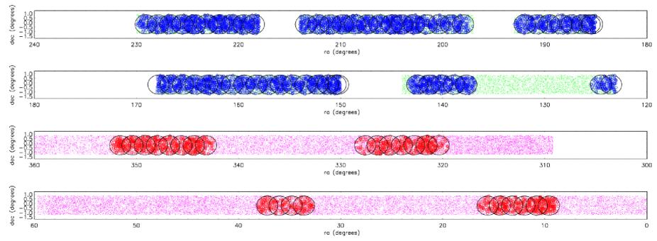
Figure 1: A sky map of the 2SLAQ observations. The upper two panels show the NGC, the lower two panels form the SGC. The black circles represent the 2dF fields observed. Green and pink dots are the NGC and SGC QSO candidates, respectively. The (blue and red) points represent the positions of the (NGC and SGC) spectroscopically confirmed QSOs.

The QSO observations were performed simultaneously with those of the LRGs. 200 2dF fibres were allocated to the LRGs and 200 to the QSO observations (Cannon et al., 2006). The LRG fibres then link to the 2dF “red spectrograph” and the QSO fibres to the “blue spectrograph”. Each block of 10 consecutive fibres along the edge of the 2dF field connects to a different spectrograph, alternately blue and red. Therefore, the QSO completeness mask in each 2dF pointing shows a “dented structure” along the edge of the field, due to the fact that the fibres are limited to an angle of $14^{\circ}$ (see, e.g. Richards et al., 2005). The probability of a given QSO/LRG candidate being assigned a 2dF fibre depends on its priority. The assigned priorities of the objects in the input catalogue (see table 1) will affect the likelihood that those objects will be observed. Objects with higher priority will have a higher likelihood to be assigned a 2dF fibre.

Objects	Priority
Guide stars	$9$
Main sample LRGs, sparsely sampled	$8$
Remaining main sample LRGs	$7$
$g>20.5$ QSOs, sparsely sampled	$6$
Remaining $g>20.5$ QSOs	$5$
Extra LRGs and high-$z$ QSOs	$4$
$g<20.5$ QSOs	$3$
Previously observed objects with good id	$1$

Table 1: 2dF priorities. Objects with higher priorities have a higher likelihood of being assigned a 2dF fibre.

Tables 2 and 3 show the number of QSOs, narrow emission line galaxies (NELGs) and stars that were observed. $Q1$ and $Q2$ refer to the identification quality: $Q1$ are objects with good identification quality and $Q2$ refer to objects with lower identification quality (see section 2.3 of Croom et al. 2004 for further details on quality identification flags). Overall, the sky density of QSO candidates in $138.4$ deg^-2 and that of confirmed QSOs is $44.7$ deg^-2.

ID	All	Q1	Q2
QSOs	$6680\ (57.89\%)$	$6482\ (56.17\%)$	$198\ (1.72\%)$
NELGs	$2077\ (18.00\%)$	$2043\ (17.71\%)$	$34\ (0.29\%)$
stars	$1829\ (15.85\%)$	$1604\ (13.90\%)$	$225\ (1.95\%)$
TOTAL	$10586\ (92.20\%)$	$10129\ (88.15\%)$	$457\ (4.05\%)$

Table 2: Number of QSOs in the NGC 2SLAQ strip.

ID	All	Q1	Q2
QSOs	$2378(49.68\%)$	$2282(47.67\%)$	$96(2.01\%)$
NELGs	$905(18.91\%)$	$881(18.40\%)$	$24(0.50\%)$
stars	$835(17.44\%)$	$739(15.44\%)$	$96(2.01\%)$
TOTAL	$4118(86.02\%)$	$3902(81.51\%)$	$216(4.51\%)$

Table 3: Number of QSOs in the SGC 2SLAQ strip.

As we are observing faint QSOs, we also expect them to have a higher space density than that achieved from other, previous surveys, such as the 2QZ or the SDSS. This is evident from the wedge plot in Fig. 2, which shows the radial projection of the 2SLAQ NGC strip (in pink). The QSOs observed from the 2QZ and SDSS DR4 (Adelman-McCarthy et al., 2006) datasets are also shown in the wedge plot, in blue and cyan squares, respectively.

,

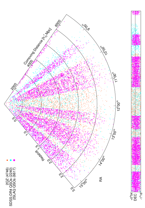
Figure 2: This shows a wedge of the sky region covered by the 2SLAQ QSO survey. The other two QSO surveys that have partial coverage in the same area are shown for comparison. The number in brackets gives the total number of QSOs with $z<3$ per survey in this region. The comoving distance is computed assuming a $\Omega_{m}^{0}=0.3$, $\Omega_{\Lambda}^{0}=0.7$, $h=0.7$ cosmology.

3 QSO clustering

Completeness issues within a 2dF pointing must be taken into account when constructing the angular mask used to generate a random set of points, which is necessary to measure QSO clustering from the 2SLAQ survey. The completeness in each pointing depends on two factors: (i) the coverage completeness, given by the fraction of QSO candidates that were assigned a 2dF fibre; and (ii) the spectroscopic completeness, representing the fraction of observed candidates which have good redshift quality. In addition, one needs to calculate the excess probability of finding a QSO in overlapping 2dF pointings.

The fact that the 2dF instrument cannot place two fibres any closer than $\sim 30$ arcsec means that an additional incompleteness can potentially lead to an artificial deficit of close QSO pairs in 2dF surveys. To make an approximate correction for these effects, one can measure the angular correlation function, $w(\theta)$ (e.g. Hawkins et al., 2003). Comparing this to the angular correlation measured in the total input catalogue allows one to estimate the average deficit of close pairs at small angular separations. As shown by Croom et al. (2001), this deficit is negligible in the 2QZ sample. In the 2SLAQ sample, however, the deficit of pairs can, potentially, constitute a bigger bias. This is due to the fact that, in contrast to what happens in the 2QZ survey, the 2SLAQ QSOs are assigned a lower observational priority than the main sample LRGs. Therefore, the QSO-assigned fibres will only be positioned in areas allowed by the underlying angular distribution of the LRG fibres. Fig. 3 shows the $w(\theta)$ measurements of the 2QZ+2SLAQ sample and the 2SLAQ and 2QZ samples separately. In order to better distinguish between the errorbars, the 2SLAQ values are offset by a shift of $\Delta\theta=+0.02$ and the 2QZ $w(\theta)$ points by a shift of $-0.02$. To account for the fibre-collision effects in the clustering of the 2SLAQ QSOs, we followed the method applied in previous work to the Two-degree Field Galaxy Redshift (2dFGRS) survey data (Hawkins et al., 2003): the number of QSO pairs at a given separation is assigned a weight that depends on the QSO’s angular separation. Since the QSO sample spans a wide redshift range, the input catalogue is expected to show zero correlation at all angular separations $w(\theta)\sim 0$, $\forall\theta$. In this case, the weight assigned to each QSO pair using the method of Hawkins et al. (2003) is $1/(1+w(\theta))$. The “imprint” of the LRG angular distribution on the QSO fibres, due to these having been assigned a low 2dF priority, is also accounted for: when generating the random catalogue for the determination of the correlation functions of the 2SLAQ QSO sample, any random point has a zero probability of lying closer than $30$ arcsec to any observed LRG. Although these effects have been considered, they have negligible effect on our clustering results.

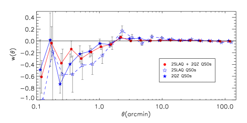
Figure 3: The angular correlation function measured for the 2QZ survey (solid blue stars and solid blue line), the 2SLAQ QSO survey (open blue stars and dashed blue line) and the 2QZ and 2SLAQ QSO surveys combined (red circles and line). The $w(\theta)$ measurements are very similar in both cases and show that the deficit of pairs seen at the smallest scales is not significant at typical QSO-QSO comoving separations. Note that the 2QZ values are offset by a shift of $\Delta\theta=-0.02$ and the 2SLAQ values by a shift of $\Delta\theta=+0.02$.

Equally as relevant is the radial completeness, which also needs to be accurately described by the unclustered, or “random” distribution. Fig. 4 shows the ($0.3<z<2.9$) redshift distribution of the 2QZ and 2SLAQ QSOs, in $\Delta z=0.13$ bins. The red line represents the 2SLAQ NGC while the blue line the 2SLAQ SGC. The green and pink lines are the $z$-distributions of the 2QZ NGC and 2QZ SGC QSOs, respectively. Dashed lines also show the polynomial fits to those distributions that were used to generate the random distribution.

The 2QZ survey comprises $22416$ (id quality 1) QSOs in the redshift range $0.3<z<2.9$ ($9982$ in the NGC and $12434$ in the SGC). The 2SLAQ QSO sample, when imposing faint magnitude cuts ($20.5<g<21.85$) in addition to these $z$-cuts, comprises a total of $6374$ QSOs ($4574$ in the NGC and $1800$ in the SGC). The fact that the 2SLAQ $N(z)$ is steeper, at low-$z$, is possibly due to QSO contamination by host galaxies, affecting the colour selection of fainter QSOs. The median redshift of the 2QZ+2SLAQ sample is $<z>=1.50$.

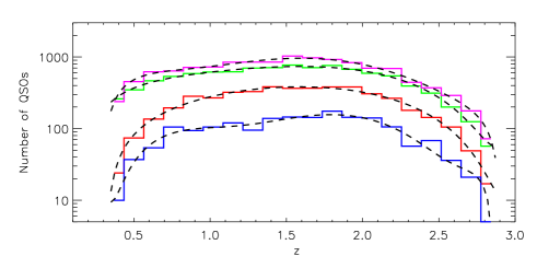
Figure 4: 2SLAQ QSO and 2QZ $N(z)$. Red line is the NGC and the blue line the SGC. The green line represents the 2QZ NGC and the pink line the 2QZ SGC. Also shown, as dashed lines, are the polynomial fits that were used to model the radial distribution of the random points.

After generating a random catalogue we can then combine the new 2SLAQ QSO sample with the 2QZ sample, and compute the QSO clustering by means of correlation functions. We start by estimating $\xi(s)$, the 2-point correlation function measured in $z$-space. This is presented in Fig. 5 (filled red circles). The estimator used to measure $\xi(s)$ is the Hamilton (1993) estimator :

$$\xi(s)=\frac{<\mathrm{DD}(s)><\mathrm{RR}(s)>}{<\mathrm{DR}(s)>^{2}}-1,$$ (1)

where $<\mathrm{DD}(s)>$, $<\mathrm{DR}(s)>$, $<\mathrm{RR}(s)>$ are the mean number of QSO-QSO, QSO-random and random-random pairs at separation $s$. For comparison, also shown is the previously determined 2QZ $\xi(s)$ (da Ângela et al., 2005), the 2SLAQ QSO $\xi(s)$ and also the $\xi(s)$ measurements of the 2SLAQ LRG sample (Ross et al., 2006). To make the plot clearer, we have offset the 2QZ and 2SLAQ $\xi(s)$ points by a factor of $0.02$ and $-0.02$, respectively.

Including the 2SLAQ QSO sample does not affect the shape of the previously measured 2QZ $\xi(s)$. The $\xi(s)$ measured from both samples, including or not the 2SLAQ QSOs, are indeed very similar. We have verified the statistical weight of including the 2SLAQ sample by comparing the number of QSO-QSO pairs at separations $<20\,h^{-1}{\rm Mpc}$, and verified that the combined 2QZ+2SLAQ sample has $\sim 65\%$ more QSO-QSO pairs within $20\,h^{-1}{\rm Mpc}$ than the 2QZ sample alone. This gain also includes the contribution of the cross pairs between the 2SLAQ and 2QZ samples, on the NGC strip. The 2SLAQ LRGs have a higher clustering amplitude than the 2SLAQ QSOs. At smaller scales the two samples also differ in the shape of their correlation functions. This is probably due to the different $z$-space distortions that affect the LRGs and the 2QZ and 2SLAQ QSOs, a contributing factor to which will be the higher redshift errors of the QSOs.

Also shown are two different 2QZ $\xi(s)$ models, obtained by da Ângela et al. (2005). The dashed line is the best fitting 2QZ power-law model, in the range $5<s<50\,h^{-1}{\rm Mpc}$ ($\xi(s)=(s/6.50)^{-1.89}$), and the solid line is the $\xi(s)$ model obtained from convolving a double power-law $\xi(r)$ model (Eq. 2) with the $z$-space distortions parameterised by $<~{}w_{z}^{2}>^{1/2}=800\,{{\rm km}}\,{{\rm s}}^{-1}$ and $\beta(z)=0.32$.

$$\xi(r)=\left\{\begin{array}[]{l}(r/6.00)^{-1.45},\ \ r<10\,h^{-1}{\rm Mpc}\\ \vskip 6.0pt plus 2.0pt minus 2.0pt\cr(r/7.25)^{-2.30},\ \ r>10\,h^{-1}{\rm Mpc}\end{array}\right.$$ (2)

It can be seen that the model is still a good description of the joint QSO $\xi(s)$ measurements, indicating that the 2SLAQ QSOs should have a similar real-space clustering and be subjected to the same dynamical distortions as the 2QZ QSOs. The fitting of these models does not take into consideration the correlations between the errors at different separations. However, da Ângela (2006) showed that taking into account the full covariance matrix when fitting the 2QZ $\xi(s)$ does not affect the $s_{0}$ and $\gamma$ values by more than $1\sigma$.

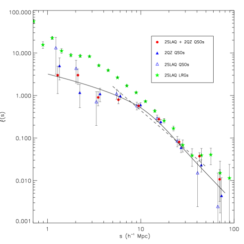
Figure 5: The red circles show the $\xi(s)$ measured from the 2SLAQ and 2QZ samples and the blue triangles the 2QZ results (from da Ângela et al., 2005). The $\xi(s)$ measurements are very similar, both in amplitude and shape. The green stars show the 2SLAQ LRG measurements (Ross et al., 2006). The dashed and solid lines show two models: the best fitting 2QZ $5<s<50\,h^{-1}{\rm Mpc}$ power law (dashed); and the double power law $\xi(r)$ model, “distorted” by dynamical motions parameterised by $<w_{z}^{2}>^{1/2}=800\,{{\rm km}}\,{{\rm s}}^{-1}$ and $\beta(z)=0.32$. Note that the $\xi(s)$ values from the individual 2SLAQ and 2QZ samples have been offset by $\log\Delta s$ of $0.02$ and $-0.02$, respectively.

The errors shown in Fig. 5 are “jacknife” estimates, estimated by splitting the 2QZ+2SLAQ sample in $16$ subsamples. We compared the jacknife and Poisson error estimates in our $\xi(s)$ computation. The Poisson error estimates should, in principle, provide a fair description of the uncertainty for the 2QZ QSO clustering measurements (Hoyle, 2000; da Ângela et al., 2005). Here we test this hypothesis for the new sample containing the 2QZ and 2SLAQ QSOs. We divide up the overall 2QZ+2SLAQ dataset into $16$ subsamples and compute $\xi(s)$ in the overall set minus each of the $16$ subsamples in turn. The $16$ measurements of $\xi(s)$ are then combined as follows, in order to obtain the jacknife error (e.g. Myers et al., 2005):

$$\sigma_{\mathrm{jacknife}}=\sqrt{\sum_{i=1}^{N}\frac{\mathrm{DR}_{i}(s)}{\mathrm{DR}_{tot}(s)}(\xi_{i}(s)-\xi_{tot}(s))^{2}}$$ (3)

where $N$ is the total number of subsamples ($16$, in this case); the subscript $i$ refers to the whole dataset minus subsample $i$; and $tot$ refers to the whole 2QZ+2SLAQ QSO sample. The “$\mathrm{DR}$ ratio” accounts for the fact that the subsamples may not necessarily contain exactly the same number of QSOs. Fig 6 shows the ratio between the jacknife and the Poisson errors. It can be seen that, on all scales, Poisson errors underestimate the uncertainty on the clustering measurements, especially at the largest scales. On scales $2\lower 3.14302pt\hbox{$\sim$}\hbox to0.0pt{\hss\raise 1.72218pt\hbox{$<$}}$ $s\lower 3.14302pt\hbox{$\sim$}\hbox to0.0pt{\hss\raise 1.72218pt\hbox{$<$}}$ $4\,h^{-1}{\rm Mpc}$, the two estimates are quite similar, but on $4\lower 3.14302pt\hbox{$\sim$}\hbox to0.0pt{\hss\raise 1.72218pt\hbox{$<$}}$ $s\lower 3.14302pt\hbox{$\sim$}\hbox to0.0pt{\hss\raise 1.72218pt\hbox{$<$}}$ $20\,h^{-1}{\rm Mpc}$ scales, where most of the clustering signal is obtained, the jacknife errors are, on average, $1.25$ times bigger than Poisson errors (dotted line). At larger scales, where there are fewer QSO independent pairs, the Poisson estimates largely under-predict the true error estimate as has been previously discussed, (e.g. Shanks & Boyle, 1994; Myers et al., 2005).

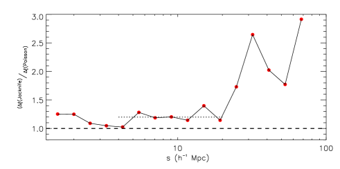
Figure 6: Red circles and solid line show the ratio jacknife and Poisson $\xi(s)$ errors. Poisson errors seem to under-predict the uncertainty in $\xi(s)$ at all scales, and considerably at the largest scales. At intermediate, $4\lower 3.14302pt\hbox{$\sim$}\hbox to0.0pt{\hss\raise 1.72218pt\hbox{$<$}}$ $s\lower 3.14302pt\hbox{$\sim$}\hbox to0.0pt{\hss\raise 1.72218pt\hbox{$<$}}$ $20\,h^{-1}{\rm Mpc}$ scales, the ratio of the two error estimates is approximately constant and $\sim 1.25$ (dotted line).

Fig. 7 shows the projected correlation function measured from the 2QZ+2SLAQ sample (red circles). This is very similar to the previous 2QZ measurement (da Ângela et al. 2005, blue triangles, offset by a factor of $\log\Delta\sigma=0.02$). The open blue triangles represent the $w_{p}(\sigma)/\sigma$ values for the 2SLAQ ensemble alone (offset by a factor of $\log\Delta\sigma=-0.02$) and the green stars represent the more strongly clustered 2SLAQ LRGs (Ross et al., 2006). The solid line is the $\sigma$-projection of the double power-law $\xi(r)$ model which was found to be a good description of the 2QZ $\xi(r)$. The relation between $w_{p}(\sigma)$ and $\xi(r)$ is given by:

$$w_{p}(\sigma)=2\int_{\sigma}^{\infty}\frac{r\xi(r)}{\sqrt{r^{2}-\sigma^{2}}}dr$$ (4)

The dashed line corresponds to the projection of a power law $\xi(r)$ model, given by $\xi(r)=(r/4.96)^{-1.85}$.

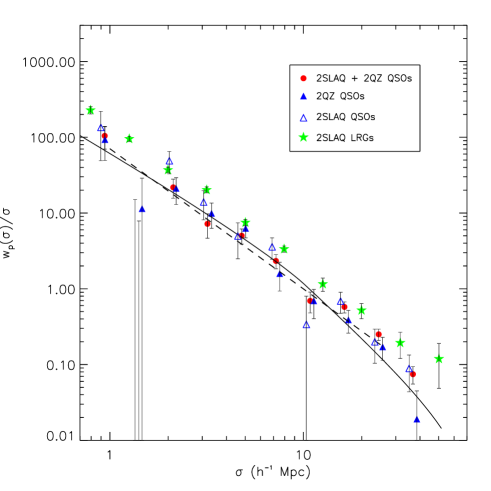
Figure 7: The red circles are the $w_{p}(\sigma)/\sigma$ measurements for the 2QZ+2SLAQ sample. These are very similar to those of the 2QZ sample alone (blue triangles; da Ângela et al., 2005). The green stars represent the higher clustered LRG sample from the 2SLAQ survey (Ross et al., 2006). The models shown represent the projection of a single (dashed line) and a double (solid line) power law models. Note that the $w_{p}(\sigma)/\sigma$ values from the individual 2QZ and 2SLAQ samples have been offset by $\log\Delta\sigma$ of $0.02$ and $-0.02$, respectively.

The fact that the 2SLAQ survey targeted faint QSOs is not only an advantage for studies of the luminosity-dependence of QSO clustering, but also for $z$-space distortion analyses. The higher spatial density of the combined QSO sample should, in principle, improve our statistics when studying $z$-space distortions, and, in particular, the estimation of $\Omega_{m}^{0}$ and $\beta(z)$ from dynamical and geometrical $\xi(\sigma,\pi)$ distortions. The $\xi(\sigma,\pi)$ measured from the whole QSO sample is shown in Fig. 8 (solid contours). The dashed lines refer to the 2QZ measurement.

Figure 8: $\xi(\sigma,\pi)$ measured for the 2QZ+2SLAQ sample (solid contours) and for the 2QZ sample alone (dashed contours). The two measurements are very similar.

4 Parameter constraints from redshift-space distortions

There are basically two mechanisms leading to dynamical $z$-space distortions. As structures grow through gravity, the infall of objects to higher-density regions contributes to the measured redshifts. If these are assumed to be solely due to the Hubble flow, then the large-scale distribution will appear flatter, or thinner, along the line of sight, thus “distorting” the clustering signal. At smaller scales, the random peculiar motions of the objects will also contribute to the measured redshifts, and hence distort the measured clustering signal for close pairs of objects. If the distribution of distant objects has, on average, a spherically symmetric clustering pattern in real space, but large velocity dispersion, then the clustering signal measured in $z$-space will be smeared along the line-of-sight. These features are often referred to as “fingers-of-God”, and are commonly seen as elongated structures in radial wedge plots of distant galaxy surveys, such as the 2dFGRS.

Peculiar velocities are not the only effect leading to anisotropies in the clustering pattern. As shown by Alcock & Paczynski (1979), if one assumes a cosmology different from the true, underlying cosmology of the Universe to convert redshifts into distances, the effect on separations along the line of sight differs from that affecting the separation in the angular coordinate. As a consequence, the clustering signal might appear elongated (or squashed) in the redshift direction. As shown by those authors these geometric distortions can be a powerful cosmological test, namely to determine $\Omega_{m}^{0}$.

Due to their significance at high-$z$, these potential geometric distortions have been used to constrain cosmological parameters using QSO catalogues (e.g. Outram et al., 2004); 21 cm maps of the epoch of reionisation (Nusser, 2005) or the Lyman $\alpha$ forest (Becker et al., 2004).

However, and as discussed in detail in Ballinger et al. (1996), it is sometimes not trivial to disentangle the effects of geometric distortions from those caused by peculiar velocities. If both the infall parameter $\beta$ and cosmological parameters as $\Omega_{m}^{0}$ or $\Omega_{\Lambda}^{0}$ are left as free variables, we expect to see a degeneracy between the anisotropies caused by the large scale infall and the geometric distortions. Those authors define a “flattening factor”, which determines, as a function of redshift and cosmology, the level of asymmetry expected to be seen as a result of geometric distortions, and found that its value is degenerate with that of $\beta$.

The fitting of the dynamical and geometrical distortions in $\xi(\sigma,\pi)$ is described in detail in section 7.7 of da Ângela et al. (2005). In summary:

1) for a given value of $\beta(z)$, a $\xi(\sigma,\pi)$ model is generated in a chosen test cosmology, through (Matsubara & Suto, 1996):

$$\xi(\sigma,\pi) = \left(1+\frac{2}{3}\beta(z)+\frac{1}{5}\beta(z)^{2}\right)\xi_{0}(r)P_{0}(\mu)$$ (5)

$$- \left(\frac{4}{3}\beta(z)+\frac{4}{7}\beta(z)^{2}\right)\xi_{2}(r)P_{2}(\mu)$$ (6)

$$+ \frac{8}{35}\beta(z)^{2}\xi_{4}(r)P_{4}(\mu),$$ (7)

where $\mu$ is now the cosine of the angle between $r$ and $\pi$ and $P_{l}(\mu)$ are the Legendre polynomials of order $l$. $\xi_{0}(r)$, $\xi_{2}(r)$ and $\xi_{4}(r)$ are the moments of order $0$, $2$ and $4$ of the linear $\xi(r)$ and their form depends on the $\xi(r)$ model adopted. In general, they are given by (Matsubara & Suto, 1996):

$$\xi_{2l}(r)=\frac{(-1)^{l}}{r^{2l+1}}\left(\int_{0}^{r}xdx\right)^{l}x^{2l}\left(\frac{d}{dx}\frac{1}{x}\right)^{l}x\xi(x)$$ (8)

2) The $\xi(\sigma,\pi)$ model is then convolved with the pairwise peculiar velocity distribution to include the small scale $z$-space effects due to the random motions of the QSOs:

$$\xi(\sigma,\pi)=\int_{-\infty}^{\infty}\xi^{\prime}(\sigma,\pi-w_{z}(1+z)/H(z))f(w_{z})dw_{z},$$ (9)

where the pairwise velocity distribution $f(w_{z})$ can be well described by a Gaussian (Ratcliffe, 1996):

$$f(w_{z})=\frac{1}{\sqrt{2\pi}<w_{z}^{2}>^{1/2}}\exp\left(-\frac{1}{2}\frac{|w_{z}|^{2}}{<w_{z}^{2}>}\right)$$ (10)

3) Then, the separations $\sigma$ and $\pi$ are scaled to the same cosmology that was assumed to measure the actual data. The final model for $\xi(\sigma,\pi)$ is then compared to the data.

The relation between the separations $\sigma$ and $\pi$ in the test and assumed cosmologies (referred to by the subscripts $t$ and $a$, respectively) is the following (Ballinger et al., 1996):

$$\sigma_{t}=f_{\perp}\sigma_{a}=\frac{B_{t}}{B_{a}}\sigma_{a}$$ (11)

$$\pi_{t}=f_{\parallel}\pi_{a}=\frac{A_{t}}{A_{a}}\pi_{a}$$ (12)

where $A$ and $B$ are defined as (for spatially flat cosmologies):

$$A=\frac{c}{H_{0}}\frac{1}{\sqrt{\Omega_{\Lambda}^{0}+\Omega_{m}^{0}(1+z)^{3}}}$$ (13)

$$B=\frac{c}{H_{0}}\int_{0}^{z}\frac{dz^{\prime}}{\sqrt{\Omega_{\Lambda}^{0}+\Omega_{m}^{0}(1+z^{\prime})^{3}}}.$$ (14)

In the linear regime, the correlation function in the assumed cosmology will be the same as the correlation function in the test cosmology, given that the separations are scaled appropriately. i.e.:

$$\xi_{t}(\sigma_{t},\pi_{t})=\xi_{a}(\sigma_{a},\pi_{a}).$$ (15)

4) This method is repeated for different test cosmologies and values of $\beta(z)$.

Given the similarities between the $\xi(\sigma,\pi)$ contours in Fig. 8, in addition to very similar $\xi(s)$ and $w_{p}(\sigma)$ measurements, we would not expect the constraints put on $\beta(z)$ and $\Omega_{m}^{0}$ from the 2QZ+2SLAQ dynamical distortions to differ from those obtained from the 2QZ sample alone (da Ângela et al., 2005), assuming that all the underlying assumptions remain the same (e.g., $\xi(r)$ shape and amplitude, velocity dispersion, scale-independent bias). We now repeat the method adopted for fitting the 2QZ dynamical and geometrical distortions, but also utilising the new 2SLAQ ensemble. The question now arises if the same $\xi(r)$ model should be assumed, or if the velocity dispersion of the QSOs should still be fixed at $800\,{{\rm km}}\,{{\rm s}}^{-1}$. It can be seen in Figs. 5 and 7 that the 2QZ double power-law $\xi(r)$ model is still a good description of both $\xi(s)$ and $w_{p}(\sigma)$ measurements for the combined sample. As the 2QZ and 2SLAQ samples have similar $N(z)$ we would not expect to see clustering differences between them due to redshift evolution. Any potential clustering difference between both sets would be due to the different luminosity of the samples. However, as suggested by both observations (e.g. Croom et al., 2005; Adelberger & Steidel, 2005; Porciani & Norberg, 2006; Myers et al., 2006), and simulations (Lidz et al., 2006; Hopkins et al., 2006) and, more importantly, as we shall see later in this paper, QSO clustering is very weakly luminosity-dependent. We therefore assume the same double power-law $\xi(r)$ prescription as used for the 2QZ sample. We also assume the same velocity dispersion as for the 2QZ sample alone. It is not unlikely that the 2SLAQ QSOs would have, on average, a different velocity dispersion. As pointed out by Berlind et al. (2003), Yoshikawa et al. (2003), or Tinker et al. (2006), galaxies can be a biased tracer of the dark matter velocity distribution, just as they are of the dark matter spatial distribution. However, as found for the 2dFGRS galaxies and predicted by HOD (Halo occupation distribution) models (Tinker et al., 2006), the expected difference for $M_{b_{J}}\lower 3.14302pt\hbox{$\sim$}\hbox to0.0pt{\hss\raise 1.72218pt\hbox{$<$}}$ $-20$ is not significant. In addition, as most of the $z$-error is due to measurement error rather than intrinsic velocity dispersion (Croom et al., 2005), we chose to continue assuming $<w_{z}^{2}>^{1/2}=800\,{{\rm km}}\,{{\rm s}}^{-1}$.

The fit to the distortions in $\xi(\sigma,\pi)$ was performed with the same assumptions and over the same range of scales as in the previous 2QZ analysis. The result is shown in Fig. 9. As expected, the contours are indeed tighter than the ones obtained when fitting only the 2QZ $\xi(\sigma,\pi)$. This is due to the increased number of pairs, not only from the 2SLAQ sample alone but also from the cross-pairs in the NGC between the two ensembles, as they probe overlapping volumes. Also shown are the $1\sigma$ and $2\sigma$ confidence levels predicted from clustering evolution and linear theory of density perturbations (dashed lines). The dotted line is, as usual, the $1\sigma$ joint confidence levels from both constraints. The best fitting values are $\Omega_{m}^{0}=0.25_{-0.07}^{+0.09}$, $\beta(z)=0.60_{-0.11}^{+0.14}$, corresponding to a $\chi^{2}_{min}=1.02$ (12 d.o.f.). Although these results favour a somewhat higher value of $\beta$ than the previous 2QZ only $\xi(\sigma,\pi)$ constraint, both obtained results are self-consistent, within the associated errors. We should point out that the size of the error bars does not take into account any potential correlation between $\xi(\sigma,\pi)$ bins but this is expected to be small. Finally the above derived values for $\Omega_{m}^{0}$ and $\beta$ imply a value of the QSO bias of $b(z=1.4)=1.5\pm 0.2$ which is slightly lower than, but not inconsistent with, the value of $b(z=1.4)\approx 2$ derived below from purely the QSO clustering amplitude.

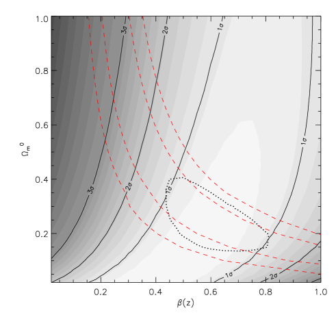
Figure 9: Confidence levels in the $[\Omega_{m}^{0},\beta(z)]$ plane obtained from fitting the 2QZ and 2SLAQ $\xi(\sigma,\pi)$ $z$-space distortions (solid lines and shaded contours). Dashed lines show the $1\ \sigma$ and $2\ \sigma$ constraints from linear theory evolution. The dotted contour is the $1\ \sigma$ joint confidence level.

5 Luminosity-redshift degeneracy

A few recent works have looked at the evolution of QSO clustering (e.g. Croom et al., 2005; Porciani et al., 2004; Myers et al., 2006). These suggest an increase of QSO clustering amplitude with redshift, a trend which is more significant at $z\lower 3.14302pt\hbox{$\sim$}\hbox to0.0pt{\hss\raise 1.72218pt\hbox{$>$}}$ $1.6$. This evolution contrasts with that expected from a long-lived QSO population model, or linear theory predictions, which generally predict a decrease of clustering amplitude with increasing redshift (Croom et al., 2001; Croom et al., 2005). The range of magnitudes covered by the QSO surveys used in these studies has not fully permitted the study of the luminosity dependence of QSO clustering. However, the combination of the 2QZ and 2SLAQ samples probably sees its greatest scientific contribution precisely in the range of luminosities it probes and for the first time allows a more rigorous determination of the QSO clustering dependence on luminosity. Croom et al. (2002) have used the 2QZ sample alone for this purpose. Their results suggest that additional, fainter data, such as those obtained for 2SLAQ, are essential to pursue this goal.

To estimate the $b_{J}$ band absolute magnitude, $M_{b_{J}}$, we compute:

$$M_{b_{J}}(z)=b_{J}-K_{b_{J}}(z)-A_{b_{J}}+5-5\log(d),$$ (16)

where $b_{J}$ is the apparent magnitude, $K_{b_{J}}$ the k-correction in the $b_{J}$ magnitude, $A_{b_{J}}$ the dust correction and $d$ the luminosity distance that corresponds to the redshift $z$, measured in parsecs. The value of the k-correction was taken from Cristiani & Vio (1990). The galactic dust correction, $A_{b_{J}}$ is determined through: $A_{b_{J}}=4.035E(B-V)$ (Schlegel et al., 1998).

The above formula is used to determine the absolute magnitude of the 2QZ QSOs. To include the dust correction when determining the absolute magnitude of the 2SLAQ QSOs, one subtracts the $g$ magnitude galactic extinction ($g_{red}$) at the QSO’s coordinates from the observed apparent magnitude ($g$): $g^{\prime}=g-g_{red}$, where $g^{\prime}$ is the dust-corrected $g$-band QSO magnitude. The other subtlety in combining the two QSO samples is accounting for the relation between the observed $b_{J}$ and $g$ magnitudes. However, this becomes quite simple as the transmissivity curves of the filters have a significant overlap and the same zero-point. Thus, we can treat these bands as being equivalent (Richards et al., 2005). Hereafter, and for the sake of simplicity, we shall refer to the QSO absolute magnitudes for both samples as if they had been measured in the $b_{J}$ band, and represent both of them as $M_{b_{J}}$. Therefore, the 2SLAQ QSOs’ absolute magnitude is determined by:

$$M_{b_{J}}(z)\approx g^{\prime}-K_{b_{J}}(z)+5-5\log(d),$$ (17)

where $g^{\prime}$ already includes the dust correction in the $g$ band.

Fig. 10 shows how the 2QZ and 2SLAQ are distributed in the $[M_{b_{J}},z]$ plane. The 2QZ QSOs are shown in red and the 2SLAQ in blue. The cyan lines represent the adopted 2QZ $b_{J}<20.85$ and 2SLAQ $20.5<g<21.85$ magnitude cuts. The QSO samples span the $z$-range $0.3<z<2.9$. The yellow line shows how $M_{b_{J}}^{*}$ changes with $z$. We adopted a second-order polynomial model to determine $M_{b_{J}}^{*}(z)$ (Boyle et al., 2000; Croom et al., 2004; Richards et al., 2005):

$$M_{b_{J}}^{*}(z)=M_{b_{J}}^{*}(0)-2.5(k_{1}z-k_{2}z^{2})$$ (18)

We adopt the values obtained by Croom et al. (2004): $M_{b_{J}}^{*}(0)=-21.61$, $k_{1}=1.39$, $k_{2}=-0.29$. Richards et al. (2005) showed that the parameterisation of the $M_{b_{J}}^{*}(z)$ model is only marginally affected by including or not the 2SLAQ QSOs. The yellow line in Fig. 10 only extends to $z=2.2$ given the fitting range used in this parameterisation.

The flux-limited nature of these two surveys is evident in this plot. More luminous QSOs lie at higher redshifts while fainter ones have lower redshifts. This means that, unless we probe a wide window in magnitude-space with our QSO surveys, it will be intrinsically hard to determine how QSO physical properties change with luminosity, for a fixed redshift. By combining the 2SLAQ and 2QZ samples we are widening the magnitude window and hence making it possible to determine the dependence of QSO clustering on luminosity, free of any evolutionary effects.

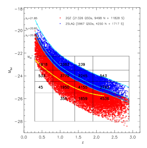
Figure 10: Magnitude and redshift bins adopted for 2QZ and 2SLAQ QSOs. The numbers in each division of the “grid” are the numbers of 2QZ and 2SLAQ QSOs in the specific $z$ and $M_{b_{J}}$ ranges.

Fig. 10 also shows how, using the two surveys together, we can look at a specific redshift range and determine the QSO clustering in different magnitude samples. This “vertical approach” to the $[M_{b_{J}},z]$ distribution is possibly more physically justifiable than simply analysing QSO clustering dependence on redshift or apparent magnitude. Tests of models where comparisons at fixed luminosity are required certainly need as full coverage as possible of the luminosity-redshift plane. Indeed, the long-lived QSO model has been easiest to test in previous samples, since comparing intrinsically low luminosity QSOs at low redshift with high luminosity QSOs at high redshift makes more sense in a PLE model where the two are hypothesised to be directly related. These results have been used to argue against a long-lived model for QSOs with the 2QZ results of $\xi_{20}$ (see equn. 19 below) appearing to rise, if anything, rather than fall with increasing redshift (Croom et al., 2004). However, the low redshift ($z\approx 0.02$) IRAS selected Seyfert 1 and 2 results of Georgantopoulos & Shanks (1994) give $\xi_{20}=0.52\pm 0.13$ in good agreement with the low redshift SDSS AGN results of Wake et al. (2004) which give $\xi_{20}=0.48\pm 0.03$ and adding these relatively high amplitude points to Fig. 21a of Croom et al. (2004) may make the clustering case against the long-lived model less strong. We note also that the low value of $\xi_{20}=0.22\pm 0.08$ measured for the cross-correlation of low luminosity QSOs with Lyman-break galaxies at z=2.5 by Adelberger & Steidel (2005) also goes against the trend for higher clustering amplitudes for higher redshift QSOs. But whatever the hypothesis for QSO lifetime, the extended luminosity range of the 2SLAQ sample means that we can now test the generic prediction of these ‘high peaks’ bias models for higher clustering amplitudes for more luminous, rare QSOs at fixed redshift.

6 Clustering as a function of magnitude and redshift

Dividing up the QSO samples into magnitude and redshift bins significantly increases the error on our clustering measurements, simply due to the much smaller number of objects in each bin compared to the total number of QSOs (numbers in Fig. 10). This is also evident in Fig. 11, where we plot the $\xi(s)$ measurements in each of the panels in Fig. 10. The dashed line shows the best fitting power-law model to the overall 2QZ+2SLAQ sample, over the $3<s<50\ \,h^{-1}{\rm Mpc}$ range ($\xi(s)=(s/6.20)^{-1.66}$). The solid lines are the best power-law models to each individual $[M_{b_{J}},z]$ interval, fixing the $\xi(s)$ slope to $\gamma=1.66$ and performing a $\chi^{2}$ fit to determine the amplitude. The order of the panels in Fig. 11 is the same as in the panels presented in the $[M_{b_{J}},z]$ plane in Fig. 10.

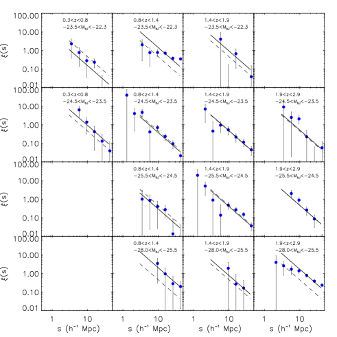
Figure 11: QSO $\xi(s)$ measured in different magnitude and redshift bins. The order of the panels is the same as that of the $[M_{b_{J}},z]$ intervals in Fig. 10. The dashed line shows the best fitting power-law to the $\xi(s)$ of the full sample. The solid line is the $\xi(s)$ power-law fit to the data in each individual panel.

By visually comparing the dashed and solid lines, we observe no dependence of QSO clustering on luminosity nor redshift. However, the size of the errorbars motivates the further use of more statistically robust tools. We therefore use the integrated correlation function up to $20\,h^{-1}{\rm Mpc}$ in order to quantify the clustering amplitude in each magnitude-$z$ bin. This quantity is then normalised to the volume contained in a $20\,h^{-1}{\rm Mpc}$ sphere:

$$\xi_{20}=\frac{3}{20^{3}}\int_{0}^{20}\xi(s)s^{2}ds$$ (19)

The choice of using $20\,h^{-1}{\rm Mpc}$ as the radius of the spheres to compute the averaged correlation function is due to the fact that this is a large enough scale for linear theory to be applied and, as shown by Croom et al. (2005), small-scale $z$-space distortions do not significantly affect the clustering measurements, when averaged over this range of scales. In addition, and as seen in Fig. 6, we can estimate the uncertainty through computing Poisson errors, and scale this by a factor of $1.25$. This estimate should provide a fair description of the uncertainty on the correlation function measurements, and significantly reduce the computing time.

We computed $\xi_{20}$ using the Hamilton estimator in each of the bins shown in Fig. 10. The results for each redshift slice are shown in the four panels in Fig. 12. Red circles show the measurements in each magnitude bin. The shaded grey area shows the $1\sigma$ $\xi_{20}$ measurement for QSOs of all luminosities in that specific redshift slice and its length indicates the total range of magnitudes included. The dashed line represents the average value of $\xi_{20}$, for all redshift and magnitude ranges. It should be pointed out that the bin sizes were chosen in such a way that the precision of the clustering measurements was maximised, and therefore the distribution of QSOs in a given $z$-slice is not constant for all magnitudes. Thus, we do not expect our $\xi_{20}$ measurements to be equidistant along the horizontal axis, as these are centred on the median values in $M_{b_{J}}$ of each bin. The top axis indicates the magnitude difference with respect to $M_{b_{J}}^{*}(<z>)$, at the median redshift of that specific “$z$ - slice”. The “rising” of the grey area as we move to higher redshifts is consistent with the results of Croom et al. (2005), who also found an increase of clustering amplitude with redshift, for the 2QZ QSOs.

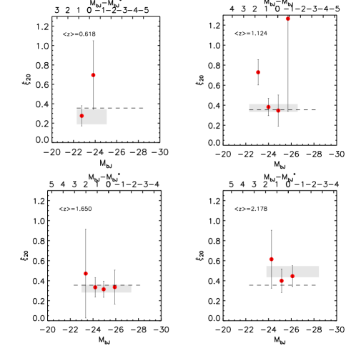
Figure 12: The four panels represent the $\xi_{20}$ measurements in different redshift bins. The median redshift of each $z$-interval is indicated in the top left of each graph. The top horizontal axis shows the absolute magnitude difference, relative to $M_{b_{J}}^{*}(<z>)$. The red circles are the $\xi_{20}$ measurements in different absolute magnitude bins, and are centred on the median values of each bin. The shaded area is the $1\sigma$ $\xi_{20}$ interval for all the QSOs in that specific redshift interval. The horizontal length of the shaded area represents the range of $M_{b_{J}}$ values of QSOs in that redshift interval.

The number of QSOs in each $M_{b_{J}}-z$ bin, indicated in Fig. 10, is now reflected in the sizes of the $\xi_{20}$ error bars. In the first, lower-$z$ panel, for instance, the $M_{b_{J}}-z$ bin with only $533$ QSOs corresponds to the $\xi_{20}$ measurement with the largest error bar. The two intermediate $z$-slices are the ones where most of the gain of the 2SLAQ is observed and the ones with highest statistical value. Our results are in agreement with the hypothesis of a luminosity-independent clustering ($\chi^{2}_{red}=1.16$, over 12 d.o.f.). The hypothesis of QSO clustering being constant with redshift and luminosity is not supported by the data ($\chi^{2}_{red}=2.50$).

7 Bias and halo masses

The $\xi_{20}$ vs. $M_{b_{J}}$ results motivate the analysis of the dependence of bias on luminosity and redshift. Croom et al. (2005) investigated the redshift evolution of QSO bias, using the 2QZ survey data. They found that the QSO bias does evolve very strongly with redshift; as the mass clustering amplitude decreases with increasing redshift, the slight upward trend observed in the 2QZ $\xi_{20}$ reveals a strong increase of bias with $z$.

Under the assumption of a scale-independent bias, the bias can be obtained through (e.g. Peebles, 1980):

$$b=\sqrt{\frac{\xi_{Q}(r)}{\xi_{\rho}(r)}}\approx\sqrt{\frac{\xi_{Q}(r,20)}{\xi_{\rho}(r,20)}},$$ (20)

where $\xi_{Q}(r,20)$ and $\xi_{\rho}(r,20)$ represent the QSO and matter real-space correlation functions, respectively, averaged in $20\,h^{-1}{\rm Mpc}$ spheres. The $z$-space and real-space correlation functions can be given by (Kaiser, 1987):

$$\xi_{Q}(s,20)=\left(1+\frac{2}{3}\beta+\frac{1}{5}\beta^{2}\right)\xi_{Q}(r,20)$$ (21)

Combining both equations and taking into account that $\beta=\Omega_{m}^{0.6}/b$ leaves us with a quadratic equation in $b$. Solving it (see Croom et al. 2005) leads to:

$$b(z)=\sqrt{\frac{\xi_{Q}(s,20)}{\xi_{\rho}(r,20)}-\frac{4\Omega_{m}^{1.2}(z)}{45}}-\frac{\Omega_{m}^{0.6}(z)}{3}$$ (22)

Therefore, we can use our $\xi_{Q}(s,20)$ measurements, represented in Fig. 12 and, together with a theoretical estimate of $\xi_{\rho}(r,20)$, determine the bias that corresponds to that theoretical assumption and the observed clustering measurements, on the assumption of a cosmological model. Our results are shown in Fig. 13. To estimate $\xi_{\rho}(r,20)$, we use the $P(k)$ non-linear estimate of Smith et al. (2003). To determine $\xi_{\rho}(r)$ we Fourier transform this $P(k)$ estimate, and integrate the result up to $s\leq 20\,h^{-1}{\rm Mpc}$ to compute $\xi_{\rho}(r,20)$. The parameters used to generate the $P(k)$ model were: $\Omega_{m}^{0}=0.3$, $\Omega_{\Lambda}^{0}=0.7$, $\Gamma=0.17$ and, for a better comparison with Croom et al.’s (2005) results, $\sigma_{8}=0.84$. This value is consistent with recent studies (e.g. Percival et al., 2002; Tytler et al., 2004), even though recent measurements also tend to suggest somewhat lower values (Spergel et al., 2006).

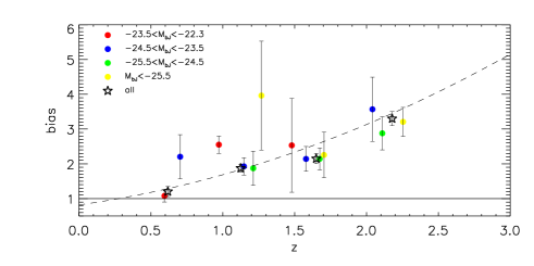
Figure 13: Bias evolution for different luminosity QSOs. The different colours refer to different absolute magnitude bins. The stars are the result for all the QSOs in each specific redshift bin. The dashed line is the empirical model of Croom et al. (2005). Each point is represented in the median redshift of all the QSOs in the specific $M_{b_{J}}$ and $z$-ranges.

The stars in Fig. 13 represent the $b$ estimates for the magnitude-integrated samples, corresponding to the shaded areas in Fig. 12. These values are very much in agreement with those found by Croom et al. (2005), using a similar method. The dashed line is the empirical description of

$$b(z)=0.53+0.289(1+z)^{2}$$

found by those authors.

The circles refer to our measurements in different magnitude bins. The red ones correspond to the faintest, $M_{b_{J}}>-23.5$ QSOs; the blue ones to the $-24.5<M_{b_{J}}<-23.5$ range; the green circles represent the QSOs with $-25.5<M_{b_{J}}<-24.5$ and the brightest, $M_{b_{J}}<-25.5$ QSOs are represented by the yellow circles. Given the size of the error bars, which are related to the errors on the associated $\xi(20)$ measurements, no categorical conclusion can be drawn, regarding the possibility of a luminosity-dependent QSO bias. The uprise in the bias values with redshift is unrelated to the different QSO luminosities, as a somewhat positive trend occurs for all QSOs irrespective of their magnitude. This is not entirely true for the brightest, $M_{b_{J}}<-25.5$, QSOs, (in yellow) for which the bias at $z\sim 1.3$ seems higher than at higher redshifts. However, given the small number of QSOs ($355$) within that redshift/magnitude range, this result would need further study.

The $b$ values for each magnitude are centred in the median redshift of the QSO sub-sample from which $b$ was determined. Hence, in each redshift bin, the $z$-displacement of different magnitude points is due to the non-uniform distribution of the QSOs in the $[M_{b_{J}},z]$ plane. That $z$-displacement, together with the colour-code on the left side of the plot, makes it easy to relate Fig. 12 to Fig. 13.

The red, 2SLAQ-dominated, fainter bin at $z\approx 1$ with a relatively small error bar deviates significantly from the empirical model of Croom et al. (2005). However, the overall trend is conservatively consistent with a luminosity-independent QSO bias.

The bias of the QSOs is related to the mass of the dark matter halo they inhabit. In a Gaussian random field the higher the fluctuation threshold the higher the clustering amplitude of fluctuations. Therefore, by measuring the clustering of QSOs we can infer the mass of the haloes the QSOs inhabit. The formalism relating bias and halo mass was firstly developed by Mo & White (1996), who assumed a spherical collapse model. This was then extended to more complicated geometries, such as ellipsoidal collapse, by Sheth et al. (2001). In the analysis in this work the latter will be the adopted formalism. According to these authors, the bias can be related to the dark halo mass by:

$$b(M_{\mathrm{DMH}},z) = 1+\left.\frac{1}{\sqrt{a}\delta_{c}(z)}\right[\sqrt{a}(a\nu^{2})+\sqrt{a}b(a\nu^{2})^{1-c}$$ (23)

$$- \left.\frac{(a\nu^{2})^{c}}{(a\nu^{2})^{c}+b(1-c)(1-c/2)}\right]$$

with $a=0.707$, $b=0.5$ and $c=0.6$. $\nu$ is defined as $\nu=\delta_{c}(z)/\sigma(M_{\mathrm{DMH}},z)$. $\delta_{c}$ is the critical density for collapse, and is given by: $\delta_{c}=0.15(12\pi)^{2/3}\Omega_{m}(z)^{0.0055}$ (Navarro et al., 1997). $\sigma(M_{\mathrm{DMH}},z)=\sigma(M_{\mathrm{DMH}})G(z)$, where $\sigma(M_{\mathrm{DMH}})$ is the rms fluctuation of the density field on the mass scale with value $M_{\mathrm{DMH}}$ and $G(z)$ is the linear growth factor (Peebles, 1984; Carroll et al., 1992). $\sigma(M_{\mathrm{DMH}})$ can hence be computed as:

$$\sigma(M_{\mathrm{DMH}})^{2}=\frac{1}{2\pi^{2}}\int_{0}^{\infty}k^{2}P(k)w(kr)^{2}dk$$ (24)

where $P(k)$ is the power spectrum of density perturbations and $w(kr)$ is the Fourier transform of a spherical top hat, which can be given by (Peebles, 1980):

$$w(kr)=3\frac{\sin(kr)-kr\cos(kr)}{(kr)^{3}}$$ (25)

where the radius $r$ is related to the mass by:

$$r=\left(\frac{3M_{\mathrm{DMH}}}{4\pi\rho_{0}}\right)^{1/3},$$ (26)

and $\rho_{0}=\Omega_{m}^{0}\rho_{crit}^{0}$ is the present mean density of the Universe, given by $\rho_{0}=2.78\times 10^{11}\Omega_{m}^{0}h^{2}M_{\odot}$ Mpc^-3.

Here, we adopt a linear form of the power spectrum, $P(k)=P_{0}T(k)^{2}k^{n}$, where $P_{0}$ is simply a normalisation parameter that depends on $\sigma_{8}$ and $T(k)$ is the transfer function, which we describe through the analytical formula of Bardeen et al. (1986).

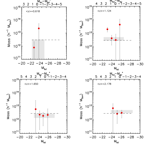
Figure 14: The four panels show the $M_{\mathrm{DMH}}$ estimates in different redshift bins. The median redshift of each $z$-interval is indicated in the top left of each graph. The top horizontal axis shows the magnitude difference relative to $M_{b_{J}}^{*}(<z>)$. The red circles show the dark matter halo mass measurements in different absolute magnitude bins, and are centred on the median values of each bin. The shaded area is the $1\sigma$ interval for the $M_{\mathrm{DMH}}$ value of all QSOs in that specific redshift interval. The horizontal length of the shaded area represents the range of $M_{b_{J}}$ values for the QSOs in the redshift interval. The dashed line shows the average $M_{\mathrm{DMH}}$ at all redshifts.

The results of performing this analysis using our determination of the bias is shown in Fig. 14. The panels show the dark matter halo mass associated with different luminosity QSOs, in the same redshift intervals as those plotted in Fig. 12. The horizontal axes show the QSO absolute magnitude (bottom), and its difference relative to $M_{b_{J}}^{*}$ (top axis), similarly to Fig. 12. In each panel, the red circles represent the $M_{\mathrm{DMH}}$ measurements in different magnitude bins, with error bars being the uncertainties corresponding to those obtained in our previous $b(z)$ estimates. The increase in the relative errors in Fig. 14 as compared to Figs. 12, 13 is due to the relatively flat slope of the $\sigma(M_{DMH})$ relation for the $\Lambda CDM$ model as obtained from equn. 24. The shaded areas represent the $1\sigma$ $M_{\mathrm{DMH}}$ confidence levels when estimating the masses associated with all QSOs, irrespective of their luminosities.

We find that, at all redshifts, QSOs seem to inhabit $M_{\mathrm{DMH}}\sim 3\times 10^{12}h^{-1}M_{\odot}$ haloes (dashed line), very much in agreement with what was found by Croom et al. (2005). As pointed out by those authors, this result appears to disfavour the picture of a long-lived QSO population. As the dark matter halo masses grow, with decreasing redshift, we would expect to see lower-$z$ QSOs in more massive haloes, if that were the case. The fact that we do not, means that at consecutive redshift intervals, we may not be observing the same QSO population, but rather distinct sets of objects. However, this conclusion is based on the 2QZ and 2SLAQ results alone and so the caveat made at the end of Section 5 about the higher clustering amplitudes measured by other authors for low redshift AGN still applies.

We also find, through our results, no evidence for $M_{\mathrm{DMH}}$ segregation with QSO magnitude at fixed redshift. All the values seem to be consistent with a flat $M_{\mathrm{DMH}}-M_{b_{J}}$ trend, indicating that QSOs seem to live in $\sim 10^{12}h^{-1}M_{\odot}$ haloes, independently of their luminosity. This behaviour is inconsistent with simple, ‘high peaks’, models of QSO biasing where rare, luminous QSOs might be expected to occupy higher mass haloes.

8 Estimating black hole masses for different luminosity QSOs

Several models and theoretical studies have been developed to try to determine the relation between the mass of the dark matter halo and the mass of the black holes associated with the observed QSOs. Here we will consider the two possible evolutionary scenarios considered by Wyithe & Loeb (2005a), both based on the results of Ferrarese (2002): 1. a correlation exists between the dark matter halo mass ($M_{\mathrm{DMH}}$) and the black hole mass ($M_{\mathrm{BH}}$) (Ferrarese, 2002) and this relation is unevolving with redshift; 2. instead, the correlation between the bulge velocity dispersion (or circular velocity) and the black hole mass (Ferrarese & Merritt, 2000; Gebhardt et al., 2000) is assumed to be unevolving with redshift. We can then estimate the black hole masses associated with different luminosity QSOs, given that we know the mass of the haloes that they inhabit, and thus determine if indeed more luminous QSOs are associated with more massive black holes. For each of these two evolutionary scenarios, and following Ferrarese (2002) and Croom et al. (2005), we will consider three possibilities for the dark matter halo profile, which affect each of assumed scenarios differently. We will consider: a) an isothermal dark matter profile; b) a NFW (Navarro et al., 1997) profile and c) a profile inferred from weak lensing studies (Seljak, 2002), which, for the sake of simplicity, we will refer to as the “lensing” profile.

When assuming a $z$-independent $M_{\mathrm{BH}}-M_{\mathrm{DMH}}$ correlation, the three possible (a), b) and c)) halo profiles correspond to the following relations (Ferrarese, 2002):

1. a) Isothermal profile:

$$\frac{M_{\mathrm{BH}}}{10^{8}M_{\odot}}\sim 0.027\left(\frac{M_{\mathrm{DMH}}}{10^{12}M_{\odot}}\right)^{1.82}$$ (27)

1. b) NFW profile:

$$\frac{M_{\mathrm{BH}}}{10^{8}M_{\odot}}\sim 0.1\left(\frac{M_{\mathrm{DMH}}}{10^{12}M_{\odot}}\right)^{1.65}$$ (28)

1. c) “Lensing” profile:

$$\frac{M_{\mathrm{BH}}}{10^{8}M_{\odot}}\sim 0.67\left(\frac{M_{\mathrm{DMH}}}{10^{12}M_{\odot}}\right)^{1.82}$$ (29)

If we assume a $z$-independent correlation between the black hole mass and the circular velocity in the associated bulges (Shields et al. 2003, 2.), then other relations are obtained. Following Croom et al. (2005) and Wyithe & Loeb (2005a), the equivalent relations between the dark matter halo mass and the black hole mass are given by:

$$M_{\mathrm{BH}}=e\left(\frac{M_{\mathrm{DMH}}}{10^{12}M_{\odot}}\right)^{2/3}\left(\frac{\Delta\Omega_{m}^{0}}{18\pi^{2}\Omega_{m}(z)}\right)^{5/6}(1+z)^{5/2}$$ (30)

where $\Delta$ has the form:

$$\Delta=18\pi^{2}+82\left(\Omega_{m}(z)-1\right)-39\left(\Omega_{m}(z)-1\right)^{2}$$ (31)

The constant $e$ is related to the halo density profile. Different values of $e$ will correspond to the same scenarios as considered in case 1.. Hence, and following Wyithe & Loeb (2005a), we have that:

2. a) For an isothermal profile:

$$e\sim 10^{-5.1}$$ (32)

2. b) For a NFW profile:

$$e\sim 3.7\times 10^{-5.1}$$ (33)

2. c) For the “lensing” profile:

$$e\sim 25\times 10^{-5.1}$$ (34)

Again, as in case 1., the three different possibilities considered for the density profile differ only in terms of a normalisation parameter, in this case, given by the constant $e$.

We now use relations 1. - 2., a), b) and c), to determine the mass of the black holes that correspond to our $M_{\mathrm{DMH}}$ measurements, under different assumptions, and determine if, with the current data, we can relate the black hole mass to the QSO luminosity.

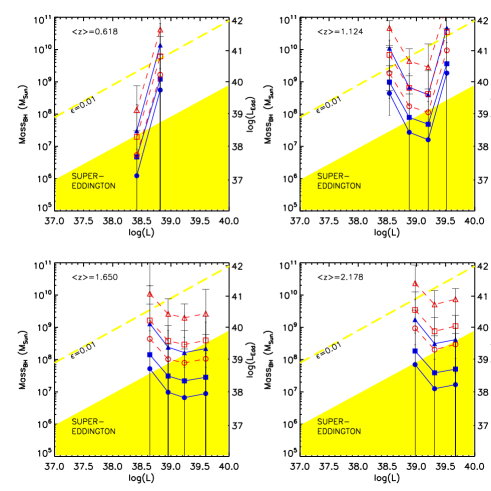
Figure 15: Black hole mass as a function of luminosity, in different redshift bins. The filled symbols and solid lines are obtained assuming a $M_{\mathrm{BH}}$ - $M_{\mathrm{DMH}}$ relation which is independent of $z$. The dashed lines and open symbols, which also correspond to the errorbars with larger tickmarks, assume a $z$-independent $M_{\mathrm{BH}}$ - $\sigma_{c}$ relation. In both cases, the circles, squares and triangles correspond to isothermal, NFW and lens-studies-based halo density profile, respectively. The points are located at the median luminosity value of the QSO sub-sample to which they correspond. On the vertical axis on the right of each panel is the equivalent Eddington luminosity scale to that for $M_{\mathrm{BH}}$, on the left. The yellow shaded area represents the super-Eddington, $L/L_{Edd}>1$, regime. The dashed yellow line corresponds to a Eddington efficiency $\epsilon=0.01$. It can be seen that some models imply super-Eddington solutions, and hence are unlikely to occur. Most of the models though, correspond to $0.01\lower 3.14302pt\hbox{$\sim$}\hbox to0.0pt{\hss\raise 1.72218pt\hbox{$<$}}$ $\epsilon\lower 3.14302pt\hbox{$\sim$}\hbox to0.0pt{\hss\raise 1.72218pt\hbox{$<$}}$ $1.0$ values.

Our results are shown in Fig. 15. Each panel shows the results obtained in a given redshift bin. Plotted is the black hole mass as a function of QSO luminosity. To determine the bolometric luminosity from $M_{b_{J}}$ we use (Croom et al., 2005):

$$L_{bol}=10^{\left(79.42-M_{b_{J}}\right)/2.66}W$$ (35)

The blue filled symbols and solid lines refer to hypothesis 1., where we assume a $M_{\mathrm{BH}}-M_{\mathrm{DMH}}$ $z$-independent relation. The red open symbols and dashed lines relate to hypothesis 2., where we assume a $M_{\mathrm{BH}}-\sigma_{c}$ relation independent of $z$. The filled and open circles show the a) estimates, in Eqs. 27 and 32, respectively, on which we assume an isothermal density profile. The squares show the results if we assume a NFW profile (b)) and the triangles if we assume the lensing profile (c)). The error bars are the corresponding uncertainties to those on the $M_{\mathrm{DMH}}$ measurements, plotted in Fig. 14. To distinguish between the error bars, the ones that refer to hypothesis 1. are represented with short tick marks, whereas the ones that refer to hypothesis 2. have longer tick marks.

For both of the assumptions, 1. or 2., the dark matter halo “lensing” density profile corresponds to more massive black holes, and the isothermal density profile corresponds to the least massive black holes, as expected. Also, it becomes evident that assuming different profiles, being it under $z$-independent $M_{\mathrm{BH}}-M_{\mathrm{DMH}}$ or $M_{\mathrm{BH}}-\sigma_{c}$ scenarios, simply “shifts” the $M_{\mathrm{BH}}-\log(L)$ relation vertically. Even though the errors associated with the $M_{\mathrm{BH}}$ are large, we can say that our values are consistent with those of Croom et al. (2005), who studied the evolution of $M_{\mathrm{BH}}$ with redshift.

Also shown, on the right-hand side vertical axis in each panel, is the Eddington luminosity. This is determined directly from the black hole mass as follows:

$$L_{Edd}=10^{39.1}\left(\frac{M_{\mathrm{BH}}}{10^{8}M_{\odot}}\right)W$$ (36)

The yellow area in the bottom of each panel represents the values of $M_{\mathrm{BH}}$ that correspond to “super-Eddington” solutions ie, $L/L_{Edd}>1$. The dashed line represents the $M_{\mathrm{BH}}-\log(L)$ relation for an Eddington efficiency of $\epsilon=L/L_{Edd}=0.01$. It can be seen that, for some of the scenarios considered, the mean efficiency is super-Eddington, in particular for models 1.a) and 1.b), ie, assuming an isothermal profile and an NFW profile, when considering that the $M_{\mathrm{BH}}-M_{\mathrm{DMH}}$ relation that does not evolve with redshift. One could argue that these relations are therefore unlikely to occur. Most of the remaining models suggest accretion efficiencies of $0.01\lower 3.14302pt\hbox{$\sim$}\hbox to0.0pt{\hss\raise 1.72218pt\hbox{$<$}}$ $\epsilon\lower 3.14302pt\hbox{$\sim$}\hbox to0.0pt{\hss\raise 1.72218pt\hbox{$<$}}$ $1$. It is somewhat unfortunate that the size of error bars do not allow us to draw conclusions regarding the significance of potential changes of black hole mass with luminosity of the associated QSO.

We averaged the data over the whole redshift range to test, through a simple $\chi^{2}$ analysis, the hypothesis that QSOs do not accrete at a fixed fraction of Eddington. Fig. 16 represents the results, by assuming the “lensing” halo density profile and $z$-independent $M_{\mathrm{BH}}$ - $\sigma_{c}$ relation (open red triangles). Also shown is the best fitting value of $\epsilon$ for that assumption.

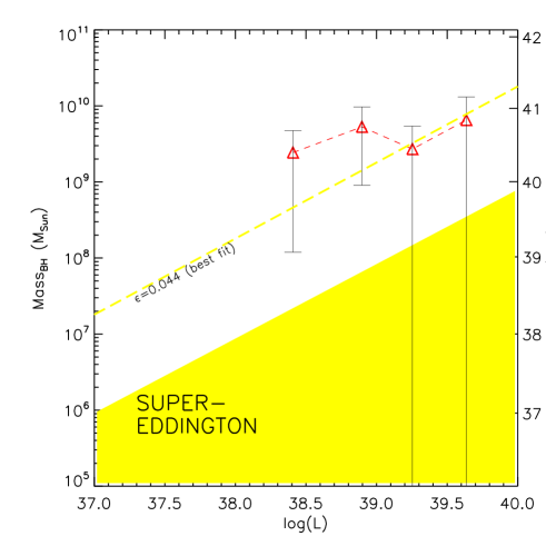
Figure 16: Black hole mass as a function of luminosity, over all redshifts. Here we assume the “lensing” halo density profile and that the $M_{\mathrm{BH}}$ - $sigma$ relation is $z$-independent. The best fitting value of $\epsilon$ is shown by the dashed yellow line.

From the “flat” trend observed in the measured $M_{\mathrm{BH}}-L$ relation, black hole mass seems approximately independent of QSO luminosity. However, this does not permit us to exclude the hypothesis that high-$z$ QSOs accrete at a fixed fraction of Eddington, as a model characterised by a constant value of $\epsilon$ is still a good fit to the data ($\epsilon=0.044$ with $\chi^{2}=1.58$; 3 d.f.). Given recent studies of Hopkins et al. (2005) and Lidz et al. (2006), who argue that bright and faint QSOs are similar sources, but observed at different stages of their activity, one could expect both luminous and faint QSOs to be associated with equally massive black holes. This would thus lead to higher values of accretion efficiency for brighter QSOs and lower for fainter QSOs. Such a model can still be in agreement with the current analysis, given the “flat” trend of the $M_{\mathrm{BH}}$ values as a function of luminosity.

Hence, our results show that, if halo mass and black hole mass are closely correlated, then we cannot reject a model where black hole mass depends on QSO luminosity and accretion efficiency. It should be noted that we have assumed that the dispersion in the black hole mass and halo mass is small. This assumption is supported by the existence of reasonably tight bulge mass - velocity dispersion relations (Tremaine et al., 2002). But clearly, if this assumption proved incorrect, then the results above would be affected by the high dispersion in the $M_{bulge}-M_{\mathrm{BH}}$ relation.

9 Conclusions

The 2SLAQ QSO survey is an important tool for QSO clustering studies. Firstly, the 2SLAQ QSO survey complements the previous 2QZ sample in terms of $z$-space distortion analyses. We have shown that a double-power law $\xi(r)$ model, which is a good description of the 2QZ real-space clustering, still describes well both the $z$-space and projected clustering measurements of the 2QZ and 2SLAQ samples combined. We fit the dynamical and geometrical distortions of the $\xi(\sigma,\pi)$ contours, extending the formalism developed by Hamilton (1992) and Matsubara & Suto (1996) to include a double-power law $\xi(r)$ model and fitting different “test” cosmologies (Alcock & Paczynski, 1979; Ballinger et al., 1996; da Ângela et al., 2005). We find that the subsequent confidence levels obtained in $\Omega_{m}^{0}$ and $\beta(z)$ are similar to those obtained when using solely the 2QZ data, but tighter due to the increased statistics from extra 2SLAQ QSO pairs, and also the additional cross-correlation pairs in the NGC 2SLAQ and 2QZ overlapping volumes. When combining these results with orthogonal contours obtained from linear theory of density perturbations, we find that $\Omega_{m}^{0}=0.25_{-0.07}^{+0.09}$, $\beta(z)=0.60_{-0.11}^{+0.14}$, similar to the values obtained from the 2QZ data alone ($\Omega_{m}^{0}=0.35_{-0.13}^{+0.19}$, $\beta(z)=0.50_{-0.15}^{+0.13}$). The new results imply $b(z=1.4)=1.5\pm 0.2$ for the QSO bias.

Secondly, the 2SLAQ QSO survey constitutes a new dataset with a potentially central role in terms of breaking the $L$-$z$ degeneracy. The sample extends $1$ magnitude fainter than the 2QZ, and spans the same $z$-range. Hence, the combination of both provides a unique dataset, as the overall magnitude range probed is similar, both at low and high-$z$. This allows us to interpret clustering results and possible luminosity-dependent measurements in different redshift bins, hence reducing any evolutionary biases. Our results are consistent with luminosity-independent QSO clustering and in agreement with those of Croom et al. (2005); QSOs seem to inhabit $\sim 3\times 10^{12}h^{-1}\ M_{\odot}$ haloes, independently of their redshift or luminosity. Our results do not show a tight correlation between halo mass and QSO luminosity at fixed redshift, as would be expected from simple ”high peaks” models of QSO biasing where fainter QSOs populate lower mass haloes.

Our $M_{\mathrm{DMH}}$ vs. $M_{b_{J}}$ results agree with the predictions of Lidz et al. (2006), whose simulation results based on the models of Hopkins et al. (2005, 2005a, 2005b, 2006) suggest that QSO luminosity may not be correlated with the mass of the host dark matter halo. The reason is that the same massive haloes host faint and bright QSOs and the difference in luminosity is due to the QSOs being observed in different periods of their lifetime. Another consequence is that QSO clustering should not correlate strongly with luminosity, again, just as shown by our data.

These authors’ analysis also support the results shown in the present paper and by Croom et al. (2005), and conclude that QSO clustering and halo mass do not evolve strongly with redshift, even though QSO bias substantially increases as we move to higher $z$. This could hint at possible anti-hierarchical QSO formation (Merloni, 2005; Cowie et al., 2003; Lidz et al., 2006), as haloes harbouring QSOs would have deeper potential wells at high-$z$ than at low-$z$, leading to more luminous black holes being observed at high-$z$ than at low-$z$. The reason for the rapid decrease of QSO bias with time is related to haloes of $\sim 10^{12}-10^{13}M_{\odot}$ corresponding to rarer, high-density-contrast peaks at higher redshift. The results of those authors also predict that a large range in QSO luminosity should correspond to a very restricted range in QSO halo masses, as our observations and measurements seem to indicate.

By assuming different density profiles for the dark matter halo and $z$-independent relations (such as $M_{\mathrm{BH}}$ - $M_{\mathrm{DMH}}$ or $M_{\mathrm{BH}}$ - $\sigma_{c}$) we can estimate the masses of the black holes associated with the QSOs. If the Eddington limit is a relevant limit for the accretion rate, and if one assumes that the $M_{\mathrm{BH}}$ - $M_{\mathrm{DMH}}$ relation is $z$-independent, then isothermal and NFW density profiles are not likely to be appropriate for the haloes these QSOs inhabit, as they predict super-Eddington accretions. This is no longer true if one assumes that the $M_{\mathrm{BH}}$ - $\sigma_{c}$ is independent of redshift, instead. Most of the other assumptions imply $\sim 10^{8}$ – $10^{10}M_{\odot}$ black holes, and accretion efficiencies of $0.01\lower 3.14302pt\hbox{$\sim$}\hbox to0.0pt{\hss\raise 1.72218pt\hbox{$<$}}$ $\epsilon\lower 3.14302pt\hbox{$\sim$}\hbox to0.0pt{\hss\raise 1.72218pt\hbox{$<$}}$ $1$. Our results suggest that at a given redshift, black hole mass is not strongly dependent on QSO bolometric luminosity, but a fixed value for the accretion efficiency is still a good fit to the data.

These results are in agreement with those of McLure & Dunlop (2004). In particular the latter measured the masses and Eddington efficiencies of high-$z$ black holes using data from the SDSS DR1, through modelling the QSO spectra. Their analysis, significantly different from that presented here, results in $M_{\mathrm{BH}}$ and efficiency $\epsilon$ values similar to those we obtained. Different relations between the black hole and dark halo masses differ almost by a scaling factor. Therefore, the trend observed in the $M_{\mathrm{BH}}-\log(L)$ plot is the same irrespective of the halo density profile and $M_{\mathrm{BH}}$ - $M_{\mathrm{DMH}}$;$M_{\mathrm{BH}}$ - $\sigma_{c}$ relation.

References

- Adelberger & Steidel (2005) Adelberger K. L., Steidel C. C., 2005, ApJ, 630, 50
- Adelman-McCarthy et al. (2006) Adelman-McCarthy J. K., et al., 2006, ApJs, 162, 38
- Alcock & Paczynski (1979) Alcock C., Paczynski B., 1979, Nat, 281, 358
- Baes et al. (2003) Baes M., Buyle P., Hau G. K. T., Dejonghe H., 2003, MNRAS, 341, L44
- Ballinger et al. (1996) Ballinger W. E., Peacock J. A., Heavens A. F., 1996, MNRAS, 282, 877
- Bardeen et al. (1986) Bardeen J. M., Bond J. R., Kaiser N., Szalay A. S., 1986, ApJ, 304, 15
- Becker et al. (2004) Becker G. D., Sargent W. L. W., Rauch M., 2004, ApJ, 613, 61
- Berlind et al. (2003) Berlind A. A., Weinberg D. H., Benson A. J., Baugh C. M., Cole S., Dav’e R., Frenk C. S., Jenkins A., Katz N., Lacey C. G., 2003, ApJ, 593, 1
- Bower et al. (2006) Bower R. G., Benson A. J., Malbon R., Helly J. C., Frenk C. S., Baugh C. M., Cole S., Lacey C. G., 2006, MNRAS, pp 659–+
- Boyle et al. (2000) Boyle B. J., Shanks T., Croom S. M., Smith R. J., Miller L., Loaring N., Heymans C., 2000, MNRAS, 317, 1014
- Boyle et al. (1988) Boyle B. J., Shanks T., Peterson B. A., 1988, MNRAS, 235, 935
- Cannon et al. (2006) Cannon R., et al., 2006, MNRAS, 372, 425
- Carroll et al. (1992) Carroll S. M., Press W. H., Turner E. L., 1992, ARAA, 30, 499
- Cowie et al. (2003) Cowie L. L., Barger A. J., Bautz M. W., Brandt W. N., Garmire G. P., 2003, ApJl, 584, L57
- Cristiani & Vio (1990) Cristiani S., Vio R., 1990, aap, 227, 385
- Croom et al. (2002) Croom S. M., Boyle B. J., Loaring N. S., Miller L., Outram P. J., Shanks T., Smith R. J., 2002, MNRAS, 335, 459
- Croom et al. (2005) Croom S. M., Boyle B. J., Shanks T., Smith R. J., Miller L., Outram P. J., Loaring N. S., Hoyle F., da Ângela J., 2005, MNRAS, 356, 415
- Croom et al. (2001) Croom S. M., Shanks T., Boyle B. J., Smith R. J., Miller L., Loaring N. S., Hoyle F., 2001, MNRAS, 325, 483
- Croom et al. (2004) Croom S. M., Smith R. J., Boyle B. J., Shanks T., Miller L., Outram P. J., Loaring N. S., 2004, MNRAS, 349, 1397
- da Ângela (2006) da Ângela J., 2006, Ph.D. Thesis, Durham University
- da Ângela et al. (2005) da Ângela J., Outram P. J., Shanks T., Boyle B. J., Croom S. M., Loaring N. S., Miller L., Smith R. J., 2005, MNRAS, 360, 1040
- Dunlop et al. (2003) Dunlop J. S., McLure R. J., Kukula M. J., Baum S. A., O’Dea C. P., Hughes D. H., 2003, MNRAS, 340, 1095
- Ferrarese (2002) Ferrarese L., 2002, ApJ, 578, 90
- Ferrarese & Merritt (2000) Ferrarese L., Merritt D., 2000, ApJl, 539, L9
- Gebhardt et al. (2000) Gebhardt K., Bender R., Bower G., Dressler A., Faber S. M., Filippenko A. V., Green R., Grillmair C., Ho L. C., Kormendy J., Lauer T. R., Magorrian J., Pinkney J., Richstone D., Tremaine S., 2000, ApJl, 539, L13
- Georgantopoulos & Shanks (1994) Georgantopoulos I., Shanks T., 1994, MNRAS, 271, 773
- Hamilton (1992) Hamilton A. J. S., 1992, ApJl, 385, L5
- Hamilton (1993) Hamilton A. J. S., 1993, ApJ, 417, 19
- Hawkins et al. (2003) Hawkins E., et al., 2003, MNRAS, 346, 78
- Hopkins et al. (2005) Hopkins P. F., Hernquist L., Cox T. J., Di Matteo T., Martini P., Robertson B., Springel V., 2005, ApJ, 630, 705
- Hopkins et al. (2005a) Hopkins P. F., Hernquist L., Cox T. J., Di Matteo T., Robertson B., Springel V., 2005a, ApJ, 630, 716
- Hopkins et al. (2005b) Hopkins P. F., Hernquist L., Cox T. J., Di Matteo T., Robertson B., Springel V., 2005b, ApJ, 632, 81
- Hopkins et al. (2006) Hopkins P. F., Hernquist L., Cox T. J., Di Matteo T., Robertson B., Springel V., 2006, ApJs, 163, 1
- Hopkins et al. (2006) Hopkins P. F., Lidz A., Hernquist L., Coil A. L., Myers A. D., Cox T. J., Spergel D. N., 2006, astro-ph/0611792
- Hoyle (2000) Hoyle F., 2000, Ph.D. Thesis, University of Durham
- Kaiser (1987) Kaiser N., 1987, MNRAS, 227, 1
- Kauffmann & Haehnelt (2000) Kauffmann G., Haehnelt M., 2000, MNRAS, 311, 576
- Kormendy & Richstone (1995) Kormendy J., Richstone D., 1995, ARAA, 33, 581
- Lidz et al. (2006) Lidz A., Hopkins P. F., Cox T. J., Hernquist L., Robertson B., 2006, ApJ, 641, 41
- Madau et al. (1996) Madau P., Ferguson H. C., Dickinson M. E., Giavalisco M., Steidel C. C., Fruchter A., 1996, MNRAS, 283, 1388
- Magorrian et al. (1998) Magorrian J., Tremaine S., Richstone D., Bender R., Bower G., Dressler A., Faber S. M., Gebhardt K., Green R., Grillmair C., Kormendy J., Lauer T., 1998, AJ, 115, 2285
- Matsubara & Suto (1996) Matsubara T., Suto Y., 1996, ApJl, 470, L1+
- McLure & Dunlop (2004) McLure R. J., Dunlop J. S., 2004, MNRAS, 352, 1390
- Merloni (2005) Merloni A., 2005, in Merloni A., Nayakshin S., Sunyaev R. A., eds, Growing Black Holes: Accretion in a Cosmological Context Anti-hierarchical Growth of Supermassive Black Holes and QSO Lifetimes. pp 453–458
- Miller et al. (2006) Miller L., Percival W. J., Croom S. M., Babić A., 2006, A& A, 459, 43
- Mo & White (1996) Mo H. J., White S. D. M., 1996, MNRAS, 282, 347
- Moore et al. (2001) Moore A. W., Connolly A. J., Genovese C., Gray A., Grone L., Kanidoris N. I., Nichol R. C., Schneider J., Szalay A. S., Szapudi I., Wasserman L., 2001, in Banday A. J., Zaroubi S., Bartelmann M., eds, Mining the Sky Fast Algorithms and Efficient Statistics: N-Point Correlation Functions. pp 71–+
- Myers et al. (2006) Myers A. D., Brunner R. J., Nichol R. C., Richards G. T., Schneider D. P., Bahcall N. A., 2006, astro-ph/0612190
- Myers et al. (2006) Myers A. D., Brunner R. J., Richards G. T., Nichol R. C., Schneider D. P., Vanden Berk D. E., Scranton R., Gray A. G., Brinkmann J., 2006, ApJ, 638, 622
- Myers et al. (2005) Myers A. D., et al., 2005, MNRAS, 359, 741
- Navarro et al. (1997) Navarro J. F., Frenk C. S., White S. D. M., 1997, ApJ, 490, 493
- Nusser (2005) Nusser A., 2005, MNRAS, 364, 743
- Outram et al. (2004) Outram P. J., Shanks T., Boyle B. J., Croom S. M., Hoyle F., Loaring N. S., Miller L., Smith R. J., 2004, MNRAS, 348, 745
- Peebles (1980) Peebles P. J. E., 1980, The large-scale structure of the universe. Research supported by the National Science Foundation. Princeton, N.J., Princeton University Press, 1980. 435 p.
- Peebles (1984) Peebles P. J. E., 1984, ApJ, 284, 439
- Percival et al. (2002) Percival W. J., et al., 2002, MNRAS, 337, 1068
- Porciani et al. (2004) Porciani C., Magliocchetti M., Norberg P., 2004, MNRAS, 355, 1010
- Porciani & Norberg (2006) Porciani C., Norberg P., 2006, astro-ph/0607348
- Ratcliffe (1996) Ratcliffe A., 1996, Ph.D. Thesis, University of Durham
- Richards et al. (2005) Richards G. T., et al., 2005, MNRAS, 360, 839
- Richstone et al. (1998) Richstone D., Ajhar E. A., Bender R., Bower G., Dressler A., Faber S. M., Filippenko A. V., Gebhardt K., Green R., Ho L. C., Kormendy J., Lauer T. R., Magorrian J., Tremaine S., 1998, Nat, 395, A14+
- Ross et al. (2006) Ross N. P., et al., 2006, astro-ph/0612400
- Schlegel et al. (1998) Schlegel D. J., Finkbeiner D. P., Davis M., 1998, ApJ, 500, 525
- Schmidt (1970) Schmidt M., 1970, ApJ, 162, 371
- Schmidt et al. (1995) Schmidt M., Schneider D. P., Gunn J. E., 1995, AJ, 110, 68
- Seljak (2002) Seljak U., 2002, MNRAS, 334, 797
- Shanks & Boyle (1994) Shanks T., Boyle B. J., 1994, MNRAS, 271, 753
- Sheth et al. (2001) Sheth R. K., Mo H. J., Tormen G., 2001, MNRAS, 323, 1
- Shields et al. (2003) Shields G. A., Gebhardt K., Salviander S., Wills B. J., Xie B., Brotherton M. S., Yuan J., Dietrich M., 2003, ApJ, 583, 124
- Shields et al. (2006) Shields G. A., Menezes K. L., Massart C. A., Vanden Bout P., 2006, ApJ, 641, 683
- Smith et al. (2003) Smith R. E., Peacock J. A., Jenkins A., White S. D. M., Frenk C. S., Pearce F. R., Thomas P. A., Efstathiou G., Couchman H. M. P., 2003, MNRAS, 341, 1311
- Spergel et al. (2006) Spergel D. N., et al., 2006, astro-ph/0603449
- Tinker et al. (2006) Tinker J. L., Norberg P., Weinberg D. H., Warren M. S., 2006, astro-ph/0603543
- Tremaine et al. (2002) Tremaine S., Gebhardt K., Bender R., Bower G., Dressler A., Faber S. M., Filippenko A. V., Green R., Grillmair C., Ho L. C., Kormendy J., Lauer T. R., Magorrian J., Pinkney J., Richstone D., 2002, ApJ, 574, 740
- Tytler et al. (2004) Tytler D., Kirkman D., O’Meara J. M., Suzuki N., Orin A., Lubin D., Paschos P., Jena T., Lin W.-C., Norman M. L., Meiksin A., 2004, ApJ, 617, 1
- Wake et al. (2004) Wake D. A., Miller C. J., Di Matteo T., Nichol R. C., Pope A., Szalay A. S., Gray A., Schneider D. P., York D. G., 2004, ApJL, 610, L85
- Wyithe & Loeb (2005a) Wyithe J. S. B., Loeb A., 2005a, ApJ, 621, 95
- Wyithe & Loeb (2005b) Wyithe J. S. B., Loeb A., 2005b, ApJ, 634, 910
- Wyithe & Padmanabhan (2006) Wyithe J. S. B., Padmanabhan T., 2006, MNRAS, 366, 1029
- York et al. (2000) York D. G., et al., 2000, AJ, 120, 1579
- Yoshikawa et al. (2003) Yoshikawa K., Jing Y. P., Borner G., 2003, ApJ, 590, 654