Coupled Cluster Treatment Of An Interpolating Triangle/Kagomé Antiferromagnet

Abstract

The coupled cluster method (CCM) is applied to a spin-half model at zero temperature which interpolates between a triangular lattice antiferromagnet (TAF) and a Kagomé lattice antiferromagnet (KAF). The strength of the bonds which connect Kagomé lattice sites is $J$, and the strength of the bonds which link the non-Kagomé lattice sites to the Kagomé lattice sites on an underlying triangular lattice is $J^{\prime}$. Our results are found to be highly converged, and our best estimate for the ground-state energy per spin for the spin-half KAF ($J^{\prime}=0$) of $-$0.4252 constitutes one of the most accurate results yet found for this model. The amount of classical ordering on the Kagomé lattice sites is also considered, and it is seen that this parameter goes to zero for values of $J^{\prime}$ very close the KAF point. Further evidence is also presented for CCM critical points which reinforce the conjecture that there is a phase near to the KAF point which is much different to that near to the TAF point ($J=J^{\prime}$).

PACS numbers: 75.10.Jm, 75.50Ee, 03.65.Ca

Our knowledge of the zero-temperature properties of lattice quantum spin systems has been enhanced by the existence of exact solutions, mostly for $s=1/2$ one-dimensional systems, and by approximate calculations for higher quantum spin number and higher spatial dimensionality. Of particular note have been the density matrix renormalisation group (DMRG) calculations DMRG1 for one-dimensional (1D) and quasi-1D spin systems, although the DMRG has, as yet, not been so conclusively applied to systems of higher spatial dimensionality. Similarly, quantum Monte Carlo (QMC) calculations qmc3 ; qmc4 at zero temperature are limited by the existence of the infamous sign problem, which in turn is often a consequence of frustration for lattice quantum spin systems. We note that for non-frustrated systems one can often determine a “sign rule” sign_rules1 ; sign_rules2 which completely circumvents the minus-sign problem.

A good example of a spin system for which, as yet, no sign rule has been proven is the spin-half triangular lattice Heisenberg antiferromagnet (TAF). The fixed-node quantum Monte Carlo (FNQMC) method taf1 has however been applied to this system with some success, although the results constitute only a variational upper bound for the energy. Other approximate methods taf2 ; taf3 ; taf4 ; taf5 have also been successfully applied to the spin-half TAF, and most, but not all, such treatments predict that about 50$\%$ of the classical Néel-like ordering on the three equivalent sublattices remains in the quantum case. In particular, series expansion results taf2 give a value for the ground-state energy of $E_{g}/N$=$-$0.551, although the corresponding value for the amount of remaining classical order of about 20$\%$ is almost certainly too low. This spin-half TAF model therefore constitutes a very challenging problem for such approximate methods. However, the spin-half Kagomé lattice Heisenberg antiferromagnet (KAF) poses an even more difficult problem, because, like the TAF, not only is it highly frustrated and no exactly provable “sign rule” exists, but also the classical ground state is infinitely degenerate. Careful finite-sized calculations kaf1 ; kaf2 ; kaf3 have however been performed for the quantum spin-half KAF, and these results indicate that none of the classical Néel-like ordering seen in the TAF remains for the quantum KAF model. The best estimate for the ground-state energy of the KAF via finite-sized calculations kaf3 stands at $E_{g}/N$=$-$0.43. Furthermore, series expansion results taf2 indicate that the ground-state of the KAF is disordered. Indeed, a variational calculation kaf4 which utilised a dimerised basis also found that the ground state of the KAF is some sort of spin liquid.

In this article we wish to apply the coupled cluster method (CCM) to a model which interpolates between the spin-half TAF and spin-half KAF models, henceforth termed the $J$–$J^{\prime}$ model (illustrated in Fig. 1). The Hamiltonian is given by

$$H=J\sum_{\langle i,j\rangle}{\bf s}_{i}\cdot{\bf s}_{j}+J^{\prime}\sum_{\{i,k\}}{\bf s}_{i}\cdot{\bf s}_{k}~{}~{},$$ (1)

where $\langle i,j\rangle$ runs over all nearest-neighbour (n.n.) bonds on the Kagomé lattice, and $\{i,k\}$ runs over all n.n. bonds which connect the Kagomé lattice sites to those other sites on an underlying triangular lattice. Note that each bond is counted once and once only. We explicitly set $J=1$ throughout this paper, and we note that at $J^{\prime}=1$ we thus have the TAF and at $J^{\prime}=0$ we have the KAF.

Figure 1: The $J$–$J^{\prime}$ model is illustrated in diagram (a), where the bonds of strength $J$ between Kagomé lattice sites are indicated by the thick solid lines and the non-Kagomé bonds of strength $J^{\prime}$ on the underlying triangular lattice sites are indicated by the “broken” lines. The triangular lattice Heisenberg antiferromagnet (TAF) is illustrated in diagram (b), and it is noted that the two models are equivalent when $J=J^{\prime}$. The quadrilateral unit cells for both cases are also illustrated. The $J$–$J^{\prime}$ model contains four sites per unit cell, whereas the TAF has only one site per unit cell.

We now briefly describe the general CCM formalism, although for further details the interested reader is referred to Refs. taf5 ; ccm1 . The exact ket and bra ground-state energy eigenvectors, $|\Psi\rangle$ and $\langle\tilde{\Psi}|$, of a general many-body system described by a Hamiltonian $H$,

$$H|\Psi\rangle=E_{g}|\Psi\rangle\;;\;\;\;\langle\tilde{\Psi}|H=E_{g}\langle\tilde{\Psi}|\;,$$ (2)

are parametrised within the single-reference CCM as follows:

$$|\Psi\rangle={\rm e}^{S}|\Phi\rangle\; \;\;\;S=\sum_{I\neq 0}{\cal S}_{I}C_{I}^{+}\;,$$ ;

$$\langle\tilde{\Psi}|=\langle\Phi|\tilde{S}{\rm e}^{-S}\; \;\;\;\tilde{S}=1+\sum_{I\neq 0}\tilde{{\cal S}}_{I}C_{I}^{-}\;.$$ ; (3)

The single model or reference state $|\Phi\rangle$ is required to have the property of being a cyclic vector with respect to two well-defined Abelian subalgebras of multi-configurational creation operators $\{C_{I}^{+}\}$ and their Hermitian-adjoint destruction counterparts $\{C_{I}^{-}\equiv(C_{I}^{+})^{\dagger}\}$. Thus, $|\Phi\rangle$ plays the role of a vacuum state with respect to a suitable set of (mutually commuting) many-body creation operators $\{C_{I}^{+}\}$. Note that $C_{I}^{-}|\Phi\rangle=0$, $\forall~{}I\neq 0$, and that $C_{0}^{-}\equiv 1$, the identity operator. These operators are furthermore complete in the many-body Hilbert (or Fock) space. Also, the correlation operator $S$ is decomposed entirely in terms of these creation operators $\{C_{I}^{+}\}$, which, when acting on the model state ($\{C_{I}^{+}|\Phi\rangle\}$), create excitations from it. We note that although the manifest Hermiticity, ($\langle\tilde{\Psi}|^{\dagger}=|\Psi\rangle/\langle\Psi|\Psi\rangle$), is lost, the normalisation conditions $\langle\tilde{\Psi}|\Psi\rangle=\langle\Phi|\Psi\rangle=\langle\Phi|\Phi\rangle\equiv 1$ are explicitly imposed. The correlation coefficients $\{{\cal S}_{I},\tilde{{\cal S}}_{I}\}$ are regarded as being independent variables, and the full set $\{{\cal S}_{I},\tilde{{\cal S}}_{I}\}$ thus provides a complete description of the ground state. For instance, an arbitrary operator $A$ will have a ground-state expectation value given as,

$$\bar{A}\equiv\langle\tilde{\Psi}|A|\Psi\rangle=\langle\Phi|\tilde{S}{\rm e}^{-S}A{\rm e}^{S}|\Phi\rangle=\bar{A}\left(\{{\cal S}_{I},\tilde{{\cal S}}_{I}\}\right)\;.$$ (4)

We note that the exponentiated form of the ground-state CCM parametrisation of Eq. (3) ensures the correct counting of the independent and excited correlated many-body clusters with respect to $|\Phi\rangle$ which are present in the exact ground state $|\Psi\rangle$. It also ensures the exact incorporation of the Goldstone linked-cluster theorem, which itself guarantees the size-extensivity of all relevant extensive physical quantities.

The determination of the correlation coefficients $\{{\cal S}_{I},\tilde{{\cal S}}_{I}\}$ is achieved by taking appropriate projections onto the ground-state Schrödinger equations of Eq. (2). Equivalently, they may be determined variationally by requiring the ground-state energy expectation functional $\bar{H}(\{{\cal S}_{I},\tilde{{\cal S}}_{I}\})$, defined as in Eq. (4), to be stationary with respect to variations in each of the (independent) variables of the full set. We thereby easily derive the following coupled set of equations,

$$\delta{\bar{H}}/\delta{\tilde{{\cal S}}_{I}}=0 \Rightarrow \langle\Phi|C_{I}^{-}{\rm e}^{-S}H{\rm e}^{S}|\Phi\rangle=0,\;\;I\neq 0\;\;;$$ (5)

$$\delta{\bar{H}}/\delta{{\cal S}_{I}}=0 \Rightarrow \langle\Phi|\tilde{S}{\rm e}^{-S}[H,C_{I}^{+}]{\rm e}^{S}|\Phi\rangle=0,\;\;I\neq 0\;.$$ (6)

Equation (5) also shows that the ground-state energy at the stationary point has the simple form

$$E_{g}=E_{g}(\{{\cal S}_{I}\})=\langle\Phi|{\rm e}^{-S}H{\rm e}^{S}|\Phi\rangle\;\;.$$ (7)

It is important to realize that this (bi-)variational formulation does not lead to an upper bound for $E_{g}$ when the summations for $S$ and $\tilde{S}$ in Eq. (3) are truncated, due to the lack of exact Hermiticity when such approximations are made. However, one can prove that the important Hellmann-Feynman theorem is preserved in all such approximations.

In the case of spin-lattice problems of the type considered here, the operators $C_{I}^{+}$ become products of spin-raising operators $s_{k}^{+}$ over a set of sites $\{k\}$, with respect to a model state $|\Phi\rangle$ in which all spins points “downward” in some suitably chosen local spin axes. The CCM formalism is exact in the limit of inclusion of all possible such multi-spin cluster correlations for $S$ and $\tilde{S}$, although in any real application this is usually impossible to achieve. It is therefore necessary to utilise various approximation schemes within $S$ and $\tilde{S}$. The three most commonly employed schemes previously utilised have been: (1) the SUB$n$ scheme, in which all correlations involving only $n$ or fewer spins are retained, but no further restriction is made concerning their spatial separation on the lattice; (2) the SUB$n$-$m$ sub-approximation, in which all SUB$n$ correlations spanning a range of no more than $m$ adjacent lattice sites are retained; and (3) the localised LSUB$m$ scheme, in which all multi-spin correlations over all distinct locales on the lattice defined by $m$ or fewer contiguous sites are retained.

Table 1: CCM results for the ground-state energy per spin and sublattice magnetisation of the TAF and KAF models using the LSUB$m$ approximation with $m=\{2,3,4,5,6\}$. CCM critical values, $J_{c}^{\prime}$, of the $J$–$J^{\prime}$ model (with $J=1$), which are themselves indicators of a phase transition point in the true system, are also given. Comparison is made in the last row with the results of other calculations.

	KAF		TAF		$J$–$J^{\prime}$
$m$	$E_{g}/{N_{K}}$	$M^{K}$	$E_{g}/N$	$M^{K}$	$J_{c}^{\prime}$
2	$-$0.37796	0.8065	$-$0.50290	0.8578	–
3	$-$0.39470	0.7338	$-$0.51911	0.8045	$-$0.683
4	$-$0.40871	0.6415	$-$0.53427	0.7273	$-$0.217
5	$-$0.41392	0.5860	$-$0.53869	0.6958	$-$0.244
6	$-$0.41767	0.5504	$-$0.54290	0.6561	$-$0.088
$\infty$	$-$0.4252	0.366	$-$0.5505	0.516	0.0$\pm$0.1
c.f.	$-$0.43.	0.0[a].	$-$0.551.	0.5.	–

For the interpolating $J$–$J^{\prime}$ model described by Eq. (1), we choose a model state $|\Phi\rangle$ in which the lattice is divided into three sublattices, denoted $\{$A,B,C$\}$. The spins on sublattice A are oriented along the negative z-axis, and spins on sublattices B and C are oriented at $+120^{\circ}$ and $-120^{\circ}$, respectively, with respect to the spins on sublattice A. Our local axes are chosen by rotating about the $y$-axis the spin axes on sublattices B and C by $-120^{\circ}$ and $+120^{\circ}$ respectively, and by leaving the spin axes on sublattice A unchanged. Under these canonical transformations,

$$s_{B}^{x}\rightarrow-\frac{1}{2}s_{B}^{x}-\frac{\sqrt{3}}{2}s_{B}^{z}\;\; \;\;s_{C}^{x}\rightarrow-\frac{1}{2}s_{C}^{x}+\frac{\sqrt{3}}{2}s_{C}^{z}\;\;,$$ ;

$$s_{B}^{y}\rightarrow s_{B}^{y}\;\; \;\;s_{C}^{y}\rightarrow s_{C}^{y}\;\;,$$ ;

$$s_{B}^{z}\rightarrow\frac{\sqrt{3}}{2}s_{B}^{x}-\frac{1}{2}s_{B}^{z}\;\; \;\;s_{C}^{z}\rightarrow-\frac{\sqrt{3}}{2}s_{C}^{x}-\frac{1}{2}s_{C}^{z}\;.$$ ; (8)

The model state $|\Phi\rangle$ now appears mathematically to consist purely of spins pointing downwards along the $z$-axis, and the Hamiltonian (for $J=1$) is given in terms of these rotated local spin axes as,

$$H = \sum_{\langle i\rightarrow j\rangle}\Bigl{\{}-{1\over 2}s_{i}^{z}s_{j}^{z}+\frac{\sqrt{3}\lambda}{4}(s_{i}^{z}s_{j}^{+}+s_{i}^{z}s_{j}^{-}-s_{i}^{+}s_{j}^{z}-s_{i}^{-}s_{j}^{z})$$

$$+ \frac{\lambda}{8}(s_{i}^{+}s_{j}^{-}+s_{i}^{-}s_{j}^{+})-\frac{3\lambda}{8}(s_{i}^{+}s_{j}^{+}+s_{i}^{-}s_{j}^{-})\Bigl{\}}$$

$$+ J^{\prime} \sum_{\{i\rightarrow k\}}\Bigl{\{}-{1\over 2}s_{i}^{z}s_{k}^{z}+\frac{\sqrt{3}\lambda}{4}(s_{i}^{z}s_{k}^{+}+s_{i}^{z}s_{k}^{-}-s_{i}^{+}s_{k}^{z}-s_{i}^{-}s_{k}^{z})$$ (9)

$$+ \frac{\lambda}{8}(s_{i}^{+}s_{k}^{-}+s_{i}^{-}s_{k}^{+})-\frac{3\lambda}{8}(s_{i}^{+}s_{k}^{+}+s_{i}^{-}s_{k}^{-})\Bigl{\}}~{}.$$

Note that $i$ and $j$ run only over the $N_{K}$ sites on the Kagomé lattice, whereas $k$ runs over those non-Kagomé sites on the (underlying) triangular lattice. $N$ indicates the total number of triangular-lattice sites, and each bond is counted once and once only. The symbol $\rightarrow$ indicates an explicit bond directionality in the Hamiltonian given by Eq. (9), namely, the three directed nearest-neighbour bonds included in Eq. (9) point from sublattice sites A to B, B to C, and C to A for both types of bond. We now perform high-order LSUB$m$ calculations for this model via a computational procedure for the Hamiltonian of Eq. (9). The interested reader is referred to Ref. taf5 for a full account of how such high-order CCM techniques are applied to lattice quantum spin systems.

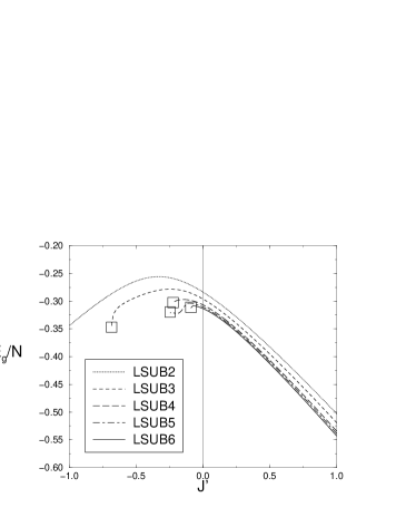
Figure 2: CCM results for the ground-state energy per spin of the $J$–$J^{\prime}$ model (with $J=1$) using the LSUB$m$ approximation with $m=\{2,3,4,5,6\}$. The boxes indicate the CCM critical points, $J^{\prime}_{c}$, and a simple extrapolation in the limit $m\rightarrow\infty$ implies that $J^{\prime}_{c}=0.0\pm 0.1$.

We note that for the CCM treatment of the $J$–$J^{\prime}$ model presented here the unit cell contains four lattice sites (see Fig. 1). By contrast, previous calculations taf5 for the TAF used a unit cell containing only a single site per unit cell. Hence, the $J$–$J^{\prime}$ model has many more “fundamental” configurations than the TAF model at equivalent levels of approximation. However, we find that those configurations which are not equivalent for the $J$–$J^{\prime}$ model but are equivalent for the TAF have CCM correlation coefficients $\{{\cal S}_{I},\tilde{\cal S}_{I}\}$ which become equal at the TAF point, $J^{\prime}=1$. Hence, the CCM naturally and without bias reflects the extra amount of symmetry of the $J$–$J^{\prime}$ model at this one particular point. This is an excellent indicator of the validity of the CCM treatment of this model. The results for the $J$–$J^{\prime}$ model at $J^{\prime}=1$ thus also exactly agree with those of a CCM previous treatment of the TAF. Our approach is now to “track” this solution for decreasing values of $J^{\prime}$ until we reach a critical value of $J^{\prime}_{c}$ at which the solution to the CCM equations breaks down. This is associated with a phase transition in the real system taf5 , and results for $J^{\prime}_{c}$ for this model are presented in Table 1. A simple “heuristic” extrapolation of these results gives a value of $J^{\prime}_{c}=0.0\pm 0.1$ for the position of this phase transition point. This result indicates that the classical three-sublattice Néel-like order, of which about 50$\%$ remains for the TAF, completely disappears at a point very near to the KAF point ($J^{\prime}=0$).

The results for the ground-state energy are shown in Fig. 2 and in Table 1. These results are seen to be highly converged with respect to each other over the whole of the region $0\leq J^{\prime}\leq 1$. A simple heuristic extrapolation may be attempted for these results for varying $J^{\prime}$ by plotting LSUB$m$ results for $m=\{3,4,5,6\}$ against $1/m^{2}$ and performing a linear extrapolation of this data as was done previously taf5 for the TAF only. These results are given in Table 1 for the KAF and TAF models. We believe that the extrapolated results are among the most accurate results for the ground-state energies of the TAF and KAF ever found.

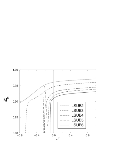
Figure 3: CCM results for the sublattice magnetisation of the $J$–$J^{\prime}$ model (with $J=1$) using the LSUB$m$ approximation with $m=\{2,3,4,5,6\}$. Note again that a simple extrapolation of LSUB$m$ critical points in the limit $m\rightarrow\infty$ implies that $J^{\prime}_{c}=0.0\pm 0.1$.

We now wish to consider how much of the original classical ordering of the model state remains for the quantum system. Previous calculations for the TAF taf5 took the average value of $s^{z}_{i}$ (after rotation of the local spin axes) where $i$ runs over all lattice sites. However, if one does this one also includes non-Kagomé lattice sites, and when $J^{\prime}=0$ the spins on this site would be effectively “frozen” to the original direction of the model state at these sites. Hence, we believe that the correct order parameter for this model is the average value of $s^{z}_{k}$ (again after rotation of the local spin axes) where $k$ runs only over the $N_{K}$ Kagomé lattice sites. We may thus write this as,

$$M^{K}=-\frac{2}{N_{K}}\sum_{k=1}^{N_{K}}s_{k}^{z}~{}~{}.$$ (10)

The results for $M^{K}$ are presented in Fig. 3 and in Table 1. Again, we extrapolate these results for the KAF by plotting LSUB$m$ results for $m=\{3,4,5,6\}$ against $1/m$ and performing a linear extrapolation of this data, as was done previously taf5 for the TAF. The extrapolated result for the KAF point probably lies too high. However, the LSUB6 result goes to zero very close to the KAF point, and so CCM results are fully consistent with the hypothesis that, unlike the TAF, the ground state of the KAF does not contain any Néel ordering.

It has been shown in this article that the CCM may be used to provide highly accurate results for the ground-state energy of the $J$–$J^{\prime}$ model (with $J=1$) which interpolates between the TAF and KAF models. Indeed, the extrapolated results for the ground-state energy for the KAF of $E_{g}/N_{K}$=$-$0.4252 and for the TAF of $E_{g}/N$=$-$0.5505 are among the most accurate yet determined for these models. Furthermore, the amount of classical ordering (evaluated on the Kagomé lattice sites only) yields results which are fully consistent with the hypothesis that the KAF is fully disordered. CCM critical points also reinforce the conjecture that the classically ordered phase evident for the TAF breaks down very near to the KAF point.

References

- (1) S.R. White and R. Noack, Phys. Rev. Lett. 68, 3487 (1992); S.R.White, Phys. Rev. Lett. 69, 2863 (1992); S.R.White, Phys. Rev. B 48 10345 (1993).
- (2) K. J. Runge, Phys. Rev. B 45, 12292 (1992); ibid. 45, 7229 (1992).
- (3) A.W. Sandvik, Phys. Rev. B 56, 11678 (1997).
- (4) R.F. Bishop, D.J.J. Farnell, and J.B. Parkinson, Phys. Rev. B 61, 6775 (2000).
- (5) R.F. Bishop and D.J.J. Farnell, in Advances in Quantum Many-Body Theory, Vol. 3, edited by R.F. Bishop, K.A. Gernoth, N.R. Walet, and Y. Xian, World Scientific, Singapore (2000) – in press.
- (6) M. Boninsegni, Phys. Rev. B 52, 5304 (1995).
- (7) R.R.P. Singh and D.A. Huse, Phys. Rev. Lett. 68, 1766 (1992).
- (8) B. Bernu, P. Lecheminant, C. Lhuillier, and L. Pierre, Phys. Scripta T49, 192 (1993); Phys. Rev. B 50, 10048 (1994).
- (9) T. Jolicoeur and J.C. LeGuillou, Phys. Rev. B 40, 2727 (1989).
- (10) C. Zeng, D.J.J. Farnell, and R.F. Bishop, J. Stat. Phys., 90, 327 (1998).
- (11) B. Bernu, P. Lechimant, and C. Lhuillier, Physica Scripta. T49. 192 (1993).
- (12) P. Lecheminant, B. Bernu, C. Lhuillier, L. Pierre, and P. Sindzingre, Phys. Rev. B 56, 2521 (1997).
- (13) C. Waldtmann, H.-U. Everts, B. Bernu, P. Sindzingre, C. Lhuillier, P. Lecheminant, and L. Pierre, Eur. Phys. J. B 2, 501 (1998).
- (14) C. Zeng and V. Elser, Phys. Rev. B 51, 8318 (1995).
- (15) R.F. Bishop, Theor. Chim. Acta 80, 95 (1991).